A survey of Tutte-Whitney polynomials - Monash University
141
A survey of Tutte-Whitney polynomials Graham Farr Faculty of IT Monash University [email protected] July 2007
Transcript of A survey of Tutte-Whitney polynomials - Monash University

A survey of Tutte-Whitney polynomials
Graham Farr
Faculty of ITMonash University
July 2007

Counting colourings
I proper colourings
Adjacent vertices receivedifferent colours
I chromatic polynomial:
P(G ; q) = # q-colourings of G

Counting colourings
I proper colourings
Adjacent vertices receivedifferent colours
I chromatic polynomial:
P(G ; q) = # q-colourings of G

Counting colourings
I proper colourings
Adjacent vertices receivedifferent colours
I chromatic polynomial:
P(G ; q) = # q-colourings of G

Counting colourings
I proper colourings
Adjacent vertices receivedifferent colours
I chromatic polynomial:
P(G ; q) = # q-colourings of G

Deletion-contraction
For any edge e:
P(G ; q) = P(G \ e; q) − P(G/e; q)
e
u v u v u = v

Partition functions: Potts models
I general q-colourings (may be improper)
Good and bad edges
I Partition function:
Z (G ;K , q) =∑
all q-colourings(not just proper)
e−K ·(# good edges)

Partition functions: Potts models
I general q-colourings (may be improper)
Good and bad edges
I Partition function:
Z (G ;K , q) =∑
all q-colourings(not just proper)
e−K ·(# good edges)

Partition functions: Potts models
I general q-colourings (may be improper)
Good and bad edges
I Partition function:
Z (G ;K , q) =∑
all q-colourings(not just proper)
e−K ·(# good edges)

Partition functions: Potts models
I general q-colourings (may be improper)
Good and bad edges
I Partition function:
Z (G ;K , q) =∑
all q-colourings(not just proper)
e−K ·(# good edges)

Partition functions: Potts models
I general q-colourings (may be improper)
Good and bad edges
I Partition function:
Z (G ;K , q) =∑
all q-colourings(not just proper)
e−K ·(# good edges)

All-terminal reliability
I Choose edges randomly: Pr(edge) = p
I Want chosen edges to contain a spanning tree
chosen edges
I Reliability:
Π(G , p) = Pr(chosen edges contain a spanning tree)

All-terminal reliability
I Choose edges randomly: Pr(edge) = p
I Want chosen edges to contain a spanning tree
chosen edges
I Reliability:
Π(G , p) = Pr(chosen edges contain a spanning tree)

All-terminal reliability
I Choose edges randomly: Pr(edge) = p
I Want chosen edges to contain a spanning tree
chosen edges
I Reliability:
Π(G , p) = Pr(chosen edges contain a spanning tree)

All-terminal reliability
I Choose edges randomly: Pr(edge) = p
I Want chosen edges to contain a spanning tree
chosen edges
I Reliability:
Π(G , p) = Pr(chosen edges contain a spanning tree)

All-terminal reliability
I Choose edges randomly: Pr(edge) = p
I Want chosen edges to contain a spanning tree
chosen edges
I Reliability:
Π(G , p) = Pr(chosen edges contain a spanning tree)

. . . etc
I flow polynomial
I # spanning trees, forests, spanning subgraphs
I weight enumerator of a linear code
I Jones polynomial of an alternating link
I . . .

. . . etc
I flow polynomial
I # spanning trees, forests, spanning subgraphs
I weight enumerator of a linear code
I Jones polynomial of an alternating link
I . . .

. . . etc
I flow polynomial
I # spanning trees, forests, spanning subgraphs
I weight enumerator of a linear code
I Jones polynomial of an alternating link
I . . .

. . . etc
I flow polynomial
I # spanning trees, forests, spanning subgraphs
I weight enumerator of a linear code
I Jones polynomial of an alternating link
I . . .

. . . etc
I flow polynomial
I # spanning trees, forests, spanning subgraphs
I weight enumerator of a linear code
I Jones polynomial of an alternating link
I . . .

. . . etc
I flow polynomial
I # spanning trees, forests, spanning subgraphs
I weight enumerator of a linear code
I Jones polynomial of an alternating link
I . . .

Tutte-Whitney polynomials
I The rank function of a graph:for all X ⊆ E :
ρ(X ) := (# vertices that meet X )− (# components of X ).
I Whitney rank generating function:
R(G ; x , y) =∑X⊆E
xρ(E)−ρ(X )y |X |−ρ(X ).
I Tutte polynomial:
T (G ; x , y) = R(G ; x − 1, y − 1).

Tutte-Whitney polynomials
I The rank function of a graph:for all X ⊆ E :
ρ(X ) := (# vertices that meet X )− (# components of X ).
I Whitney rank generating function:
R(G ; x , y) =∑X⊆E
xρ(E)−ρ(X )y |X |−ρ(X ).
I Tutte polynomial:
T (G ; x , y) = R(G ; x − 1, y − 1).

Tutte-Whitney polynomials
I The rank function of a graph:for all X ⊆ E :
ρ(X ) := (# vertices that meet X )− (# components of X ).
I Whitney rank generating function:
R(G ; x , y) =∑X⊆E
xρ(E)−ρ(X )y |X |−ρ(X ).
I Tutte polynomial:
T (G ; x , y) = R(G ; x − 1, y − 1).

The “Recipe Theorem”
Theorem(Tutte 1947 → Brylawski 1972 → Oxley & Welsh 1979)If a function f on graphs . . .
I is invariant under isomorphism,
I satisfies a deletion-contraction relation,
I is multiplicative over components(i.e., f (G1 ∪ G2) = f (G1) · f (G2)),
. . . then f is essentially a (partial) evaluation of the Tutte-Whitneypolynomial.
Example
P(G ; q) = (−1)ρ(E)qk(G)R(G ;−q,−1)

x21−1−2
2
1
-1
-2
y
chromatic
flowreliability
weight enumerator
Potts model
Joneseasy

x21−1−2
2
1
-1
-2
y
chromatic
flowreliability
weight enumerator
Potts model
Joneseasy

x21−1−2
2
1
-1
-2
y
chromatic
flow
reliability
weight enumerator
Potts model
Joneseasy

x21−1−2
2
1
-1
-2
y
chromatic
flowreliability
weight enumerator
Potts model
Joneseasy

x21−1−2
2
1
-1
-2
y
chromatic
flowreliability
weight enumerator
Potts model
Joneseasy

x21−1−2
2
1
-1
-2
y
chromatic
flowreliability
weight enumerator
Potts model
Joneseasy

x21−1−2
2
1
-1
-2
y
chromatic
flowreliability
weight enumerator
Potts model
Jones
easy

x21−1−2
2
1
-1
-2
y
chromatic
flowreliability
weight enumerator
Potts model
Joneseasy

x21−1−2
2
1
-1
-2
y
chromatic
flowreliability
weight enumerator
Potts model
Joneseasy

History
Graphs:Chrom.poly�� ��P(G ; q)
Birkhoff1912
-�� ��R(G ; x , y)
Whitney, 1935Tutte, 1947
-�� ��T (G ; x , y)
Tutte1954
-aaaa!!!!
Stat Mech:partitionfunctions
#" !
Isingmodel(q = 2)
Ising1925
-
'&$%
Pottsmodel(all q)
Potts1952
���
����Ashkin-Teller
model (q = 4)
A. & T., 1943
JJ
JJ
JJJ
Fortuin &Kasteleyn
1972-
Linear codes:weight
enumerator�� ��AC(z)
MacWilliams1963
�Greene1974
-
Network reliability:
�� ��Π(G ; p)
van Slyke &Frank, 1971
BBBBBBBBBN
Oxley &Welsh1979
Knots:Jones poly
�� ��VL(t)
Jones1985 �
�������
Thistle-thwaite1987

History
Graphs:Chrom.poly
�� ��P(G ; q)
Birkhoff1912
-�� ��R(G ; x , y)
Whitney, 1935Tutte, 1947
-�� ��T (G ; x , y)
Tutte1954
-aaaa!!!!
Stat Mech:partitionfunctions
#" !
Isingmodel(q = 2)
Ising1925
-
'&$%
Pottsmodel(all q)
Potts1952
���
����Ashkin-Teller
model (q = 4)
A. & T., 1943
JJ
JJ
JJJ
Fortuin &Kasteleyn
1972-
Linear codes:weight
enumerator�� ��AC(z)
MacWilliams1963
�Greene1974
-
Network reliability:
�� ��Π(G ; p)
van Slyke &Frank, 1971
BBBBBBBBBN
Oxley &Welsh1979
Knots:Jones poly
�� ��VL(t)
Jones1985 �
�������
Thistle-thwaite1987

History
Graphs:Chrom.poly�� ��P(G ; q)
Birkhoff1912
-�� ��R(G ; x , y)
Whitney, 1935Tutte, 1947
-�� ��T (G ; x , y)
Tutte1954
-aaaa!!!!
Stat Mech:partitionfunctions
#" !
Isingmodel(q = 2)
Ising1925
-
'&$%
Pottsmodel(all q)
Potts1952
���
����Ashkin-Teller
model (q = 4)
A. & T., 1943
JJ
JJ
JJJ
Fortuin &Kasteleyn
1972-
Linear codes:weight
enumerator�� ��AC(z)
MacWilliams1963
�Greene1974
-
Network reliability:
�� ��Π(G ; p)
van Slyke &Frank, 1971
BBBBBBBBBN
Oxley &Welsh1979
Knots:Jones poly
�� ��VL(t)
Jones1985 �
�������
Thistle-thwaite1987

History
Graphs:Chrom.poly�� ��P(G ; q)
Birkhoff1912
-�� ��R(G ; x , y)
Whitney, 1935Tutte, 1947
-�� ��T (G ; x , y)
Tutte1954
-aaaa!!!!
Stat Mech:partitionfunctions
#" !
Isingmodel(q = 2)
Ising1925
-
'&$%
Pottsmodel(all q)
Potts1952
���
����Ashkin-Teller
model (q = 4)
A. & T., 1943
JJ
JJ
JJJ
Fortuin &Kasteleyn
1972-
Linear codes:weight
enumerator
�� ��AC(z)
MacWilliams1963
�Greene1974
-
Network reliability:
�� ��Π(G ; p)
van Slyke &Frank, 1971
BBBBBBBBBN
Oxley &Welsh1979
Knots:Jones poly
�� ��VL(t)
Jones1985 �
�������
Thistle-thwaite1987

History
Graphs:Chrom.poly�� ��P(G ; q)
Birkhoff1912
-�� ��R(G ; x , y)
Whitney, 1935Tutte, 1947
-�� ��T (G ; x , y)
Tutte1954
-aaaa!!!!
Stat Mech:partitionfunctions
#" !
Isingmodel(q = 2)
Ising1925
-
'&$%
Pottsmodel(all q)
Potts1952
���
����Ashkin-Teller
model (q = 4)
A. & T., 1943
JJ
JJ
JJJ
Fortuin &Kasteleyn
1972-
Linear codes:weight
enumerator�� ��AC(z)
MacWilliams1963
�Greene1974
-
Network reliability:
�� ��Π(G ; p)
van Slyke &Frank, 1971
BBBBBBBBBN
Oxley &Welsh1979
Knots:Jones poly
�� ��VL(t)
Jones1985 �
�������
Thistle-thwaite1987

History
Graphs:Chrom.poly�� ��P(G ; q)
Birkhoff1912
-�� ��R(G ; x , y)
Whitney, 1935Tutte, 1947
-�� ��T (G ; x , y)
Tutte1954
-aaaa!!!!
Stat Mech:partitionfunctions
#" !
Isingmodel(q = 2)
Ising1925
-
'&$%
Pottsmodel(all q)
Potts1952
���
����Ashkin-Teller
model (q = 4)
A. & T., 1943
JJ
JJ
JJJ
Fortuin &Kasteleyn
1972-
Linear codes:weight
enumerator�� ��AC(z)
MacWilliams1963
�Greene1974
-
Network reliability:
�� ��Π(G ; p)
van Slyke &Frank, 1971
BBBBBBBBBN
Oxley &Welsh1979
Knots:Jones poly
�� ��VL(t)
Jones1985
��������
Thistle-thwaite1987

History
Graphs:Chrom.poly�� ��P(G ; q)
Birkhoff1912
-�� ��R(G ; x , y)
Whitney, 1935Tutte, 1947
-�� ��T (G ; x , y)
Tutte1954
-aaaa!!!!
Stat Mech:partitionfunctions
#" !
Isingmodel(q = 2)
Ising1925
-
'&$%
Pottsmodel(all q)
Potts1952
���
����Ashkin-Teller
model (q = 4)
A. & T., 1943
JJ
JJ
JJJ
Fortuin &Kasteleyn
1972-
Linear codes:weight
enumerator�� ��AC(z)
MacWilliams1963
�Greene1974
-
Network reliability:
�� ��Π(G ; p)
van Slyke &Frank, 1971
BBBBBBBBBN
Oxley &Welsh1979
Knots:Jones poly
�� ��VL(t)
Jones1985 �
�������
Thistle-thwaite1987

Complexity of computing all of R(G ; x , y)
I Graphs: #P-hard (Linial, 1986)
I Bipartite graphs: #P-hard (Linial, 1986)
I Bipartite planar graphs: #P-hard (Vertigan & Welsh, 1992)
I Planar graphs, max degree 3: #P-hard (Vertigan, 1990)
I Square grid subgraphs, max deg 3: #P-hard (GF, 2006)
I Square grid graphs: Open (in #P1)
I Bounded tree-width: p-time (Noble, 1998; Andrzejak, 1998)

Complexity of evaluating at specific points
Theorem(Jaeger, Vertigan and Welsh, 1990)The problem of determining R(G ; x , y), given a graph G, is#P-hard at all points (x , y) except those where xy = 1 and(x , y) = (0, 0), (−1,−2), (−2,−1), (−2,−2).

Generalisations
Extensions from graphs to:
I representable matroids (Smith), matroids (Tutte, Crapo),greedoids (Gordon & McMahon), Boolean functions or setsystems (GF), hyperplane arrangements (Welsh & Whittle,Ardila), semimatroids (Ardila), signed graphs (Murasugi),rooted graphs (Wu, King & Lu), K -terminal graphs (Traldi),biased graphs (Zaslavsky), matroid perspectives (LasVergnas), matroid pairs (Welsh & Kayibi), bimatroids (Kung),graphic polymatroids (Borzacchini), general polymatroids(Oxley & Whittle), . . .
. . . or extend the polynomials:
I multivariate polynomials of various kinds: variables at eachvertex (Noble & Welsh), or edge (Fortuin & Kasteleyn, Traldi,Kung, Sokal, Bollobas & Riordan, Zaslavsky, Ellis-Monaghan& Riordan, Britz).

Generalisations
Common themes:
I interesting partial evaluations
I deletion-contraction relations
I Recipe Theorems
I easier proofs
I roots
I how much of the graph is determined by the polynomial?
We now look at a generalisation to Boolean functions . . .

Generalisations
Common themes:
I interesting partial evaluations
I deletion-contraction relations
I Recipe Theorems
I easier proofs
I roots
I how much of the graph is determined by the polynomial?
We now look at a generalisation to Boolean functions . . .

Generalisations
Common themes:
I interesting partial evaluations
I deletion-contraction relations
I Recipe Theorems
I easier proofs
I roots
I how much of the graph is determined by the polynomial?
We now look at a generalisation to Boolean functions . . .

Generalisations
Common themes:
I interesting partial evaluations
I deletion-contraction relations
I Recipe Theorems
I easier proofs
I roots
I how much of the graph is determined by the polynomial?
We now look at a generalisation to Boolean functions . . .

Generalisations
Common themes:
I interesting partial evaluations
I deletion-contraction relations
I Recipe Theorems
I easier proofs
I roots
I how much of the graph is determined by the polynomial?
We now look at a generalisation to Boolean functions . . .

Generalisations
Common themes:
I interesting partial evaluations
I deletion-contraction relations
I Recipe Theorems
I easier proofs
I roots
I how much of the graph is determined by the polynomial?
We now look at a generalisation to Boolean functions . . .

Generalisations
Common themes:
I interesting partial evaluations
I deletion-contraction relations
I Recipe Theorems
I easier proofs
I roots
I how much of the graph is determined by the polynomial?
We now look at a generalisation to Boolean functions . . .

Generalisations
Common themes:
I interesting partial evaluations
I deletion-contraction relations
I Recipe Theorems
I easier proofs
I roots
I how much of the graph is determined by the polynomial?
We now look at a generalisation to Boolean functions . . .

Generalisations
Common themes:
I interesting partial evaluations
I deletion-contraction relations
I Recipe Theorems
I easier proofs
I roots
I how much of the graph is determined by the polynomial?
We now look at a generalisation to Boolean functions . . .

Rank ↔ rowspaceIncidence matrix
edges
vertices 0/1 entries· · · · · ·
...
...
E \W︷ ︸︸ ︷ W︷ ︸︸ ︷E (edge set)︷ ︸︸ ︷
−→ echelon form
0 I · · · · · · · · ·
0 0 I...
0
6
?
ρ(E \W )6
?
ρ(E )
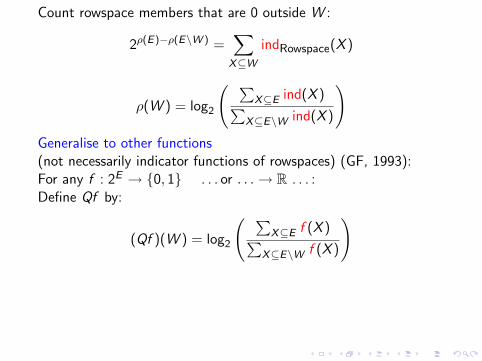
Count rowspace members that are 0 outside W :
2ρ(E)−ρ(E\W ) =∑
X⊆W
indRowspace(X )

Rank ↔ rowspaceIncidence matrix
edges
vertices 0/1 entries· · · · · ·
...
...
E \W︷ ︸︸ ︷ W︷ ︸︸ ︷E (edge set)︷ ︸︸ ︷
−→ echelon form
0 I · · · · · · · · ·
0 0 I...
0
6
?
ρ(E \W )6
?
ρ(E )
Count rowspace members that are 0 outside W :
2ρ(E)−ρ(E\W ) =∑
X⊆W
indRowspace(X )

Rank ↔ rowspaceIncidence matrix
edges
vertices 0/1 entries· · · · · ·
...
...
E \W︷ ︸︸ ︷ W︷ ︸︸ ︷E (edge set)︷ ︸︸ ︷
−→ echelon form
0 I · · · · · · · · ·
0 0 I...
0
6
?
ρ(E \W )6
?
ρ(E )
Count rowspace members that are 0 outside W :
2ρ(E)−ρ(E\W ) =∑
X⊆W
indRowspace(X )

Rank ↔ rowspaceIncidence matrix
edges
vertices 0/1 entries· · · · · ·
...
...
E \W︷ ︸︸ ︷ W︷ ︸︸ ︷E (edge set)︷ ︸︸ ︷
−→ echelon form
0 I · · · · · · · · ·
0 0 I...
0
6
?
ρ(E \W )6
?
ρ(E )
Count rowspace members that are 0 outside W :
2ρ(E)−ρ(E\W ) =∑
X⊆W
indRowspace(X )

Rank ↔ rowspaceIncidence matrix
edges
vertices 0/1 entries· · · · · ·
...
...
E \W︷ ︸︸ ︷ W︷ ︸︸ ︷E (edge set)︷ ︸︸ ︷
−→ echelon form
0 I · · · · · · · · ·
0 0 I...
0
6
?
ρ(E \W )6
?
ρ(E )
Count rowspace members that are 0 outside W :
2ρ(E)−ρ(E\W ) =∑
X⊆W
indRowspace(X )

Rank ↔ rowspaceIncidence matrix
edges
vertices 0/1 entries· · · · · ·
...
...
E \W︷ ︸︸ ︷ W︷ ︸︸ ︷E (edge set)︷ ︸︸ ︷
−→ echelon form
0 I · · · · · · · · ·
0 0 I...
0
6
?
ρ(E \W )6
?
ρ(E )
Count rowspace members that are 0 outside W :
2ρ(E)−ρ(E\W ) =∑
X⊆W
indRowspace(X )

Count rowspace members that are 0 outside W :
2ρ(E)−ρ(E\W ) =∑
X⊆W
indRowspace(X )
ρ(W ) = log2
( ∑X⊆E ind(X )∑
X⊆E\W ind(X )
)Generalise to other functions(not necessarily indicator functions of rowspaces) (GF, 1993):For any f : 2E → {0, 1} . . . or . . . → R . . . :Define Qf by:
(Qf )(W ) = log2
( ∑X⊆E f (X )∑
X⊆E\W f (X )
)
Inversion: if ρ : 2E → {0, 1} then define Q†ρ by
(Q†ρ)(V ) = (−1)|V |∑
W⊆V
(−1)|W |2ρ(E)−ρ(E\W )

Count rowspace members that are 0 outside W :
2ρ(E)−ρ(E\W ) =∑
X⊆W
indRowspace(X )
ρ(W ) = log2
( ∑X⊆E ind(X )∑
X⊆E\W ind(X )
)
Generalise to other functions(not necessarily indicator functions of rowspaces) (GF, 1993):For any f : 2E → {0, 1} . . . or . . . → R . . . :Define Qf by:
(Qf )(W ) = log2
( ∑X⊆E f (X )∑
X⊆E\W f (X )
)
Inversion: if ρ : 2E → {0, 1} then define Q†ρ by
(Q†ρ)(V ) = (−1)|V |∑
W⊆V
(−1)|W |2ρ(E)−ρ(E\W )

Count rowspace members that are 0 outside W :
2ρ(E)−ρ(E\W ) =∑
X⊆W
indRowspace(X )
ρ(W ) = log2
( ∑X⊆E ind(X )∑
X⊆E\W ind(X )
)Generalise to other functions(not necessarily indicator functions of rowspaces) (GF, 1993):
For any f : 2E → {0, 1} . . . or . . . → R . . . :Define Qf by:
(Qf )(W ) = log2
( ∑X⊆E f (X )∑
X⊆E\W f (X )
)
Inversion: if ρ : 2E → {0, 1} then define Q†ρ by
(Q†ρ)(V ) = (−1)|V |∑
W⊆V
(−1)|W |2ρ(E)−ρ(E\W )
Count rowspace members that are 0 outside W :
2ρ(E)−ρ(E\W ) =∑
X⊆W
indRowspace(X )
ρ(W ) = log2
( ∑X⊆E ind(X )∑
X⊆E\W ind(X )
)Generalise to other functions(not necessarily indicator functions of rowspaces) (GF, 1993):For any f : 2E → {0, 1} . . . or . . . → R . . . :Define Qf by:
(Qf )(W ) = log2
( ∑X⊆E f (X )∑
X⊆E\W f (X )
)
Inversion: if ρ : 2E → {0, 1} then define Q†ρ by
(Q†ρ)(V ) = (−1)|V |∑
W⊆V
(−1)|W |2ρ(E)−ρ(E\W )

Count rowspace members that are 0 outside W :
2ρ(E)−ρ(E\W ) =∑
X⊆W
indRowspace(X )
ρ(W ) = log2
( ∑X⊆E ind(X )∑
X⊆E\W ind(X )
)Generalise to other functions(not necessarily indicator functions of rowspaces) (GF, 1993):For any f : 2E → {0, 1} . . . or . . . → R . . . :Define Qf by:
(Qf )(W ) = log2
( ∑X⊆E f (X )∑
X⊆E\W f (X )
)
Inversion:
if ρ : 2E → {0, 1} then define Q†ρ by
(Q†ρ)(V ) = (−1)|V |∑
W⊆V
(−1)|W |2ρ(E)−ρ(E\W )

Count rowspace members that are 0 outside W :
2ρ(E)−ρ(E\W ) =∑
X⊆W
indRowspace(X )
ρ(W ) = log2
( ∑X⊆E ind(X )∑
X⊆E\W ind(X )
)Generalise to other functions(not necessarily indicator functions of rowspaces) (GF, 1993):For any f : 2E → {0, 1} . . . or . . . → R . . . :Define Qf by:
(Qf )(W ) = log2
( ∑X⊆E f (X )∑
X⊆E\W f (X )
)
Inversion: if ρ : 2E → {0, 1} then define Q†ρ by
(Q†ρ)(V ) = (−1)|V |∑
W⊆V
(−1)|W |2ρ(E)−ρ(E\W )

Properties of the transform Q
Basic properties:
I (Q†Qf )(V ) =f (V )
f (∅)I (QQ†ρ)(V ) = ρ(V )− ρ(∅)
I Q†QQ† = Q†
I QQ†Q = Q
Relationship with the Hadamard transform:
f (W ) :=1
2n
∑X⊆E
(−1)|W∩X |f (X )
f -QQf
Hadamard transform ↓ ↓ matroid-style dual
f -Q(Qf )∗ = Qf

Properties of the transform Q
Basic properties:
I (Q†Qf )(V ) =f (V )
f (∅)I (QQ†ρ)(V ) = ρ(V )− ρ(∅)I Q†QQ† = Q†
I QQ†Q = Q
Relationship with the Hadamard transform:
f (W ) :=1
2n
∑X⊆E
(−1)|W∩X |f (X )
f -QQf
Hadamard transform ↓ ↓ matroid-style dual
f -Q(Qf )∗ = Qf

Properties of the transform Q
Basic properties:
I (Q†Qf )(V ) =f (V )
f (∅)I (QQ†ρ)(V ) = ρ(V )− ρ(∅)I Q†QQ† = Q†
I QQ†Q = Q
Relationship with the Hadamard transform:
f (W ) :=1
2n
∑X⊆E
(−1)|W∩X |f (X )
f -QQf
Hadamard transform ↓ ↓ matroid-style dual
f -Q(Qf )∗ = Qf

Properties of the transform Q
Basic properties:
I (Q†Qf )(V ) =f (V )
f (∅)I (QQ†ρ)(V ) = ρ(V )− ρ(∅)I Q†QQ† = Q†
I QQ†Q = Q
Relationship with the Hadamard transform:
f (W ) :=1
2n
∑X⊆E
(−1)|W∩X |f (X )
f -QQf
Hadamard transform ↓ ↓ matroid-style dual
f -Q(Qf )∗ = Qf

Extending the Whitney rank generating function
R(f ; x , y) =∑X⊆E
xQf (E)−Qf (X )y |X |−Qf (X )
R1(f ; x , y) = xQf (E)∑X⊆E
(xy)−Qf (X )y |X |
Example:
E = {1, 2}
X f
∅ 1{1} 1{2} 1{1, 2} 0
R(f ; x , y) = x log2 3 + 2xy2−log2 3 + y2−log23

Extending the Whitney rank generating function
R(f ; x , y) =∑X⊆E
xQf (E)−Qf (X )y |X |−Qf (X )
R1(f ; x , y) = xQf (E)∑X⊆E
(xy)−Qf (X )y |X |
Example:
E = {1, 2}
X f
∅ 1{1} 1{2} 1{1, 2} 0
R(f ; x , y) = x log2 3 + 2xy2−log2 3 + y2−log23

Extending the Whitney rank generating function
R(f ; x , y) =∑X⊆E
xQf (E)−Qf (X )y |X |−Qf (X )
R1(f ; x , y) = xQf (E)∑X⊆E
(xy)−Qf (X )y |X |
Example:
E = {1, 2}
X f
∅ 1{1} 1{2} 1{1, 2} 0
R(f ; x , y) = x log2 3 + 2xy2−log2 3 + y2−log23

Extending the Whitney rank generating function
R(f ; x , y) =∑X⊆E
xQf (E)−Qf (X )y |X |−Qf (X )
R1(f ; x , y) = xQf (E)∑X⊆E
(xy)−Qf (X )y |X |
Example:
E = {1, 2}
X f
∅ 1{1} 1{2} 1{1, 2} 0
R(f ; x , y) = x log2 3 + 2xy2−log2 3 + y2−log23

Deletion-contraction
For e ∈ E , X ⊆ E \ {e}:
Deletion Contraction
(f \\e)(X ) =f (X ) + f (X ∪ {e})
f (∅) + f ({e}); (f //e)(X ) =
f (X )
f (∅).
Deletion-contraction rule:
R(f ; x , y) = xlog2
“1+ f ({e}
f (∅)
”R(f \\e; x , y)+y
log2
“1+ f ({e}
f (∅)
”R(f //e; x , y)

Deletion-contraction
For e ∈ E , X ⊆ E \ {e}:
Deletion Contraction
(f \\e)(X ) =f (X ) + f (X ∪ {e})
f (∅) + f ({e}); (f //e)(X ) =
f (X )
f (∅).
Deletion-contraction rule:
R(f ; x , y) = xlog2
“1+ f ({e}
f (∅)
”R(f \\e; x , y)+y
log2
“1+ f ({e}
f (∅)
”R(f //e; x , y)

Generalised Tutte-Whitney plane
x21−1−2
2
1
-1
-2
y
chromatic
clutter reliability
weight enum. nonlinear code
gen. Potts model
easy

Generalised Tutte-Whitney plane
x21−1−2
2
1
-1
-2
y
chromatic
clutter reliability
weight enum. nonlinear code
gen. Potts model
easy

Generalised Tutte-Whitney plane
x21−1−2
2
1
-1
-2
y
chromatic
clutter reliability
weight enum. nonlinear code
gen. Potts model
easy

Generalised Tutte-Whitney plane
x21−1−2
2
1
-1
-2
y
chromatic
clutter reliability
weight enum. nonlinear code
gen. Potts model
easy

Generalised Tutte-Whitney plane
x21−1−2
2
1
-1
-2
y
chromatic
clutter reliability
weight enum. nonlinear code
gen. Potts model
easy

Generalised Tutte-Whitney plane
x21−1−2
2
1
-1
-2
y
chromatic
clutter reliability
weight enum. nonlinear code
gen. Potts model
easy

Generalised Tutte-Whitney plane
x21−1−2
2
1
-1
-2
y
chromatic
clutter reliability
weight enum. nonlinear code
gen. Potts model
easy

Generalised Tutte-Whitney plane
x21−1−2
2
1
-1
-2
y
chromatic
clutter reliability
weight enum. nonlinear code
gen. Potts model
easy

Interpolating between contraction and deletion
For e ∈ E , X ⊆ E \ {e}:
Contraction
λ-minor
Deletion
(λ = 0) (λ = 1)
(f //e)(X )
(f ‖λe)(X )
(f \\e)(X )
f (X )
f (∅)
f (X ) + λf (X ∪ {e})f (∅) + λf ({e})
f (X ) + f (X ∪ {e})f (∅) + f ({e})
0 λ 1

Interpolating between contraction and deletion
For e ∈ E , X ⊆ E \ {e}:
Contraction λ-minor Deletion
(λ = 0) (λ = 1)
(f //e)(X ) (f ‖λe)(X ) (f \\e)(X )
f (X )
f (∅)f (X ) + λf (X ∪ {e})
f (∅) + λf ({e})f (X ) + f (X ∪ {e})
f (∅) + f ({e})
0 λ 1

Interpolating between contraction and deletion
For e ∈ E , X ⊆ E \ {e}:
Contraction λ-minor Deletion(λ = 0) (λ = 1)
(f //e)(X ) (f ‖λe)(X ) (f \\e)(X )
f (X )
f (∅)f (X ) + λf (X ∪ {e})
f (∅) + λf ({e})f (X ) + f (X ∪ {e})
f (∅) + f ({e})
0 λ 1

Interpolating between contraction and deletion
For e ∈ E , X ⊆ E \ {e}:
Contraction λ-minor Deletion(λ = 0) (λ = 1)
(f //e)(X ) (f ‖λe)(X ) (f \\e)(X )
f (X )
f (∅)f (X ) + λf (X ∪ {e})
f (∅) + λf ({e})f (X ) + f (X ∪ {e})
f (∅) + f ({e})
0 λ 1

Duality
Duality between deletion and contraction can be extended.
Define
λ∗ :=1− λ
1 + λ
Thenf ‖
λe = f ‖
λ∗ e
Fixed points:λ = ±
√2− 1

Duality
Duality between deletion and contraction can be extended. Define
λ∗ :=1− λ
1 + λ
Thenf ‖
λe = f ‖
λ∗ e
Fixed points:λ = ±
√2− 1

Duality
Duality between deletion and contraction can be extended. Define
λ∗ :=1− λ
1 + λ
Thenf ‖
λe = f ‖
λ∗ e
Fixed points:λ = ±
√2− 1

Duality
Duality between deletion and contraction can be extended. Define
λ∗ :=1− λ
1 + λ
Thenf ‖
λe = f ‖
λ∗ e
Fixed points:λ = ±
√2− 1

λ-rank functions
Define Q(λ)f by:
(Q(λ)f )(W ) = log2
((1 + λ∗)|V |∑
X⊆E λ|X |f (X )∑X⊆E\W λ|W∩V |(λ∗)|W∩V |f (X )
)
Duality:(Q(λ))∗ = Q(λ∗)
Inversion:
(Q†(λ)ρ)(V ) =
(−1)|V |(λ− λ∗)−|S | ×
∑W⊆V
(−1)|W |(1 + λ∗)−|W |(λ∗)|W∩V |λ|W∩V |2ρ(E)−ρ(E\W )

λ-rank functions
Define Q(λ)f by:
(Q(λ)f )(W ) = log2
((1 + λ∗)|V |∑
X⊆E λ|X |f (X )∑X⊆E\W λ|W∩V |(λ∗)|W∩V |f (X )
)
Duality:(Q(λ))∗ = Q(λ∗)
Inversion:
(Q†(λ)ρ)(V ) =
(−1)|V |(λ− λ∗)−|S | ×
∑W⊆V
(−1)|W |(1 + λ∗)−|W |(λ∗)|W∩V |λ|W∩V |2ρ(E)−ρ(E\W )

λ-rank functions
Define Q(λ)f by:
(Q(λ)f )(W ) = log2
((1 + λ∗)|V |∑
X⊆E λ|X |f (X )∑X⊆E\W λ|W∩V |(λ∗)|W∩V |f (X )
)
Duality:(Q(λ))∗ = Q(λ∗)
Inversion:
(Q†(λ)ρ)(V ) =
(−1)|V |(λ− λ∗)−|S | ×
∑W⊆V
(−1)|W |(1 + λ∗)−|W |(λ∗)|W∩V |λ|W∩V |2ρ(E)−ρ(E\W )

A continuum of λ-Whitney functions
R(λ)(f ; x , y) =∑X⊆E
xQ(λ)f (E)−Q(λ)f (X )y |X |−Q(λ)f (X )
R(λ)1 (f ; x , y) = xQ(λ)f (E)
∑X⊆E
(xy)−Q(λ)f (X )y |X |
0
R(f ; x , y)
√2− 1
(√
x +√
y)|E |
λ
R(λ)(f ; x , y)
1
R(f ; x , y)

A continuum of λ-Whitney functions
R(λ)(f ; x , y) =∑X⊆E
xQ(λ)f (E)−Q(λ)f (X )y |X |−Q(λ)f (X )
R(λ)1 (f ; x , y) = xQ(λ)f (E)
∑X⊆E
(xy)−Q(λ)f (X )y |X |
0
R(f ; x , y)
√2− 1
(√
x +√
y)|E |
λ
R(λ)(f ; x , y)
1
R(f ; x , y)

A continuum of λ-Whitney functions
R(λ)(f ; x , y) =∑X⊆E
xQ(λ)f (E)−Q(λ)f (X )y |X |−Q(λ)f (X )
R(λ)1 (f ; x , y) = xQ(λ)f (E)
∑X⊆E
(xy)−Q(λ)f (X )y |X |
0
R(f ; x , y)
√2− 1
(√
x +√
y)|E |
λ
R(λ)(f ; x , y)
1
R(f ; x , y)

Properties of the λ-Whitney function:
R(λ)(f ; x , y)
I obeys a deletion-contraction-type relation(with operations ‖
λ, ‖
λ∗ );
I contains the weight enumerator of a nonlinear code. . . but this is also in R(f ; x , y), i.e., don’t need λ;
I contains the partition function of the Ashkin-Teller modelon a graph G. . . which is not determined by R(G ; x , y),so do need λ.

Properties of the λ-Whitney function:
R(λ)(f ; x , y)
I obeys a deletion-contraction-type relation(with operations ‖
λ, ‖
λ∗ );
I contains the weight enumerator of a nonlinear code
. . . but this is also in R(f ; x , y), i.e., don’t need λ;
I contains the partition function of the Ashkin-Teller modelon a graph G. . . which is not determined by R(G ; x , y),so do need λ.

Properties of the λ-Whitney function:
R(λ)(f ; x , y)
I obeys a deletion-contraction-type relation(with operations ‖
λ, ‖
λ∗ );
I contains the weight enumerator of a nonlinear code. . . but this is also in R(f ; x , y), i.e., don’t need λ;
I contains the partition function of the Ashkin-Teller modelon a graph G. . . which is not determined by R(G ; x , y),so do need λ.

Properties of the λ-Whitney function:
R(λ)(f ; x , y)
I obeys a deletion-contraction-type relation(with operations ‖
λ, ‖
λ∗ );
I contains the weight enumerator of a nonlinear code. . . but this is also in R(f ; x , y), i.e., don’t need λ;
I contains the partition function of the Ashkin-Teller modelon a graph G
. . . which is not determined by R(G ; x , y),so do need λ.

Properties of the λ-Whitney function:
R(λ)(f ; x , y)
I obeys a deletion-contraction-type relation(with operations ‖
λ, ‖
λ∗ );
I contains the weight enumerator of a nonlinear code. . . but this is also in R(f ; x , y), i.e., don’t need λ;
I contains the partition function of the Ashkin-Teller modelon a graph G. . . which is not determined by R(G ; x , y),so do need λ.

Ashkin-Teller model (1943)I 4-colourings (may be improper): colours are (±1,±1)
+1
−1
−1
−1
+1
+1
−1
+1
Left colours:Good and bad edgesRight colours:Good and bad edgesProduct colours:Good and bad edges
I Partition function (symmetric Ashkin-Teller):ZAT(G ;K ,K ′, q) =
e(2K+K ′)|E |∑
e
−
0B@ K · (# good “left” edges)+ K · (# good “right” edges)+ K ′ · (# good “product” edges)
1CA

Ashkin-Teller model (1943)I 4-colourings (may be improper): colours are (±1,±1)
+1
−1
−1
−1
+1
+1
−1
+1
Left colours:Good and bad edges
Right colours:Good and bad edgesProduct colours:Good and bad edges
I Partition function (symmetric Ashkin-Teller):ZAT(G ;K ,K ′, q) =
e(2K+K ′)|E |∑
e
−
0B@ K · (# good “left” edges)+ K · (# good “right” edges)+ K ′ · (# good “product” edges)
1CA

Ashkin-Teller model (1943)I 4-colourings (may be improper): colours are (±1,±1)
+1
−1
−1
−1
+1
+1
−1
+1
Left colours:Good and bad edgesRight colours:Good and bad edgesProduct colours:Good and bad edges
I Partition function (symmetric Ashkin-Teller):ZAT(G ;K ,K ′, q) =
e(2K+K ′)|E |∑
e
−
0B@ K · (# good “left” edges)+ K · (# good “right” edges)+ K ′ · (# good “product” edges)
1CA

Ashkin-Teller model (1943)I 4-colourings (may be improper): colours are (±1,±1)
+1
−1
−1
−1
+1
+1
−1
+1
Left colours:Good and bad edges
Right colours:Good and bad edges
Product colours:Good and bad edges
I Partition function (symmetric Ashkin-Teller):ZAT(G ;K ,K ′, q) =
e(2K+K ′)|E |∑
e
−
0B@ K · (# good “left” edges)+ K · (# good “right” edges)+ K ′ · (# good “product” edges)
1CA

Ashkin-Teller model (1943)I 4-colourings (may be improper): colours are (±1,±1)
+1
−1
−1
−1
+1
+1
−1
+1
Left colours:Good and bad edgesRight colours:Good and bad edgesProduct colours:Good and bad edges
I Partition function (symmetric Ashkin-Teller):ZAT(G ;K ,K ′, q) =
e(2K+K ′)|E |∑
e
−
0B@ K · (# good “left” edges)+ K · (# good “right” edges)+ K ′ · (# good “product” edges)
1CA

Ashkin-Teller model (1943)I 4-colourings (may be improper): colours are (±1,±1)
+1
−1
−1
−1
+1
+1
−1
+1
Left colours:Good and bad edgesRight colours:Good and bad edges
Product colours:Good and bad edges
I Partition function (symmetric Ashkin-Teller):ZAT(G ;K ,K ′, q) =
e(2K+K ′)|E |∑
e
−
0B@ K · (# good “left” edges)+ K · (# good “right” edges)+ K ′ · (# good “product” edges)
1CA

Ashkin-Teller model (1943)I 4-colourings (may be improper): colours are (±1,±1)
+1
−1
−1
−1
+1
+1
−1
+1
Left colours:Good and bad edgesRight colours:Good and bad edges
Product colours:Good and bad edges
I Partition function (symmetric Ashkin-Teller):ZAT(G ;K ,K ′, q) =
e(2K+K ′)|E |∑
e
−
0B@ K · (# good “left” edges)+ K · (# good “right” edges)+ K ′ · (# good “product” edges)
1CA

Ashkin-Teller model (1943)
Special cases:
I K = K ′: Potts model (up to a factor)
I K ′ = 0: product of two Ising models (each q = 2)
For these, ZAT(G ) is a specialisation of R(G : x , y).
In general, ZAT(G ) is not a specialisation of R(G : x , y).Example (M. C. Gray; see Tutte (1974)):
These graphs have same R(G ; x , y), but different ZAT(G )(even in symmetric case).

λ-Tutte-Whitney plane
x21−1−2
2
1
-1
-2
y
weight enum. nonlinear code
Ashkin-Teller model
easy

λ-Tutte-Whitney plane
x21−1−2
2
1
-1
-2
y
weight enum. nonlinear code
Ashkin-Teller model
easy

λ-Tutte-Whitney plane
x21−1−2
2
1
-1
-2
y
weight enum. nonlinear code
Ashkin-Teller model
easy

λ-Tutte-Whitney plane
x21−1−2
2
1
-1
-2
y
weight enum. nonlinear code
Ashkin-Teller model
easy

λ-Tutte-Whitney plane
x21−1−2
2
1
-1
-2
y
weight enum. nonlinear code
Ashkin-Teller model
easy