A Support Vector Machine Cost Function in Simulated ...

A Support Vector Machine Cost Function in Simulated

Annealing for Network Intrusion Detection

By

Md Nasimuzzaman Chowdhury

A thesis is submitted to the Faculty of Graduate Studies of

The University of Manitoba

In the fulfillment of the requirements for the degree of

Master of Science

Department of Electrical and Computer Engineering

University of Manitoba

Winnipeg, Manitoba

Copyrights © 2018 by Md Nasimuzzaman Chowdhury

ii

Abstract

This research proposes an intelligent computational approach for feature extraction merging

Simulated Annealing (SA) and Support Vector Machine (SVM). The thesis aims to develop a

methodology that can provide a reasonable solution for meaningful extraction of data features

from a finite number of features/attributes set. Particularly, the proposed method can deal with

large datasets efficiently. The proposed methodology is analyzed and validated using two different

network intrusion dataset and the performance measures used are; detection accuracy, false

positive and false negative rate, Receiver Operation Characteristics curve, Area Under Curve

Value and F1 score. Subsequently, a comparative analysis of the proposed model with other

machine learning techniques (i.e. general SVM and decision trees) based schemes have been

performed to evaluate and benchmark the efficacy of the proposed methodology. The empirically

validated results show that proposed SA-SVM based model outperforms the general SVM and

decision tree-based detection schemes based on performance measures such as detection

accuracy, false positive and false negative rates, Area Under Curve Value and F1 score.

iii

Acknowledgments

First, I would like to thank and praise Almighty ALLAH for my life, unconditional love and,

granting me to do M.Sc. at the University of Manitoba.

I would like to express my gratitude to Prof. Dr. Ken Ferens for his supervision in my research on

cybersecurity and his guidance during my M.Sc. Study at the University of Manitoba. I would like

to thank him from the core of my heart for being a great advisor and an awesome person to work

with. Thank you very much once again for tolerating my inexperienced questions so long.

I would like to thank my parents Md Fazlul Karim Chowdhury & Amina Banu Chowdhury for

inspiring me to do M.Sc. abroad and teaching how to keep faith in me. Also, for their numerous

support, I am finally at the end of the program.

Finally, I would love to thank from the bottom of my heart to my wife Dr. Kashfia Shafiq for her

inspiration, motivation, and support for completing the research program.

iv

Dedication

I dedicate this work to my parents, my sister and my wife for their love and moral support. I also

dedicate this thesis to my supervisor Professor Dr. Ken Ferens for his innovative ideas and

supervision during the entire period of the master’s program.

v

Table of Contents

Abstract .......................................................................................................................................... ii

Acknowledgments ........................................................................................................................ iii

Dedication ..................................................................................................................................... iv

Chapter 1 ....................................................................................................................................... 1

1. Introduction ....................................................................................................................... 1

1.1. Thesis Statement and Overview ................................................................................... 6

1.2. The contribution of the Thesis ...................................................................................... 7

1.3. Outline of the thesis ...................................................................................................... 7

Chapter 2 ....................................................................................................................................... 8

2. Background Research ....................................................................................................... 8

Chapter 3 ..................................................................................................................................... 16

3. Background of Machine Learning Algorithm .............................................................. 16

3.1. Support Vector Machine ............................................................................................. 16

3.2. Simulated Annealing .................................................................................................. 19

3.3. Decision Trees ............................................................................................................ 22

Classification and Regression Tree (CART) .................................................................... 22

Chapter 4 ..................................................................................................................................... 24

4. Background on Network Intrusion Detection System ................................................. 24

4.1. Network Intrusion ....................................................................................................... 24

4.2. Intrusion Detection System ........................................................................................ 25

4.3. Classification of Intrusion Detection System ............................................................. 27

4.3.1. Location of the Network System ......................................................................... 28

4.3.1.1. Host-based Intrusion Detection System ........................................................ 28

4.3.1.2. The Network-based intrusion detection system ............................................ 29

4.3.2. The functionality of the Network system ............................................................ 31

4.3.2.1. Intrusion Prevention System ......................................................................... 31

4.3.2.2. Intrusion Detection and Prevention System .................................................. 31

4.3.3. Deployment Approach ........................................................................................ 32

4.3.3.1. Single Host .................................................................................................... 32

4.3.3.2. Multiple Host ................................................................................................. 32

4.3.4. Detection Method Based Classification .............................................................. 33

4.3.4.1. Signature-Based Approach ............................................................................ 33

4.3.4.2. Anomaly-Based Approach ............................................................................ 34

vi

Chapter 5 ..................................................................................................................................... 37

5. Dataset and attack types ................................................................................................. 37

5.1. Types of Attack .......................................................................................................... 39

5.1.1. Active Attack ....................................................................................................... 39

5.2. Passive Attack............................................................................................................. 41

Chapter 6 ..................................................................................................................................... 43

6. Proposed Algorithm ........................................................................................................ 43

6.1. Initial Algorithm [85] ................................................................................................. 43

6.2. Proposed Algorithm [86] ............................................................................................ 44

Chapter 7 ..................................................................................................................................... 47

7. Experiments and Results ................................................................................................ 47

7.1. Simulation Setup for General SVM Based Detection Method ................................... 47

7.2. Simulation Setup for Proposed Algorithm (2 features) .............................................. 53

7.3. Simulation Setup for The Proposed Algorithm (3 features) ....................................... 57



7.6. Simulation Setup for The Proposed Algorithm using UNB Dataset (3 features) ....... 78

7.7. Performance Comparison ........................................................................................... 83

7.8. Performance comparison with Decision tree-based method ...................................... 87

Chapter 8 ..................................................................................................................................... 94

8. Conclusions and Future Works ..................................................................................... 94

References .................................................................................................................................... 96

vii

List of Figures

Figure 3.1: Simulated annealing diagram [50]. ............................................................................ 21

Figure 4.1: Block diagram of an IDS process. .............................................................................. 26

Figure 4.2: Factors contributing to the classification of the intrusion detection system. ............. 28

Figure 4.3: Positioning of HIDS and NIDS on a netowrk ............................................................ 29

Figure 4.4: General flowchart of the signature-based intrusion detection method. ...................... 34

Figure 4.5: General flowchart of anomaly-based detection approach. ......................................... 35

Figure 7.1: Detection accuracy of the designed model (using the initial algorithm). ................... 49

Figure 7.2: False positive & false negative rate. ........................................................................... 50

Figure 7.3: Receiver operating characteristic curve of the designed model. ................................ 51

Figure 7.4: Detection accuracy of the proposed model. ............................................................... 54

Figure 7.5: False positive & false negative rate. ........................................................................... 55

Figure 7.6: Receiver operating characteristic curve. .................................................................... 55

Figure 7.7: F1 score of the detection scheme. .............................................................................. 56

Figure 7.8: Detection accuracy of the proposed scheme. ............................................................. 60

Figure 7.9: False positive and false negative rate of the proposed scheme. ................................. 61

Figure 7.10: Receiver operating characteristic curve. .................................................................. 62

Figure 7.11: F1 score of the proposed method. ............................................................................ 63

Figure 7.12: Detection accuracy difference with the increasing number of iterations. ................ 64

Figure 7.13: Performance of the proposed scheme inside equilibrium loop. ............................... 65

Figure 7.14: Detection accuracy of equilibrium loops. ................................................................. 66

Figure 7.15: Detection accuracy using the proposed for the four-feature combination. .............. 71

Figure 7.16: False positive and negative rate................................................................................ 71

Figure 7.17: Receiver operating characteristic curve and AUC for the four-feature combination.

....................................................................................................................................................... 72

Figure 7.18: F1 score of the proposed algorithm for the four-feature combination. .................... 72

Figure 7.19: Detection accuracy of the proposed scheme for the five-feature combination. ....... 75


Figure 7.21: F1 score of 5-feature subset combination. ................................................................ 76

Figure 7.22: Receiver operation characteristic of 5-feature subset combinations. ....................... 76

Figure 7.23: Detection accuracy of the proposed scheme using the UNB dataset. ...................... 80


Figure 7.25: Receiver operation characteristics. ........................................................................... 81

Figure 7.26: F1 score of the proposed scheme. ............................................................................ 81

Figure 7.27: Performance of the initial algorithm (exhaustive search). ....................................... 84

Figure 7.28: Performance of the proposed method. ...................................................................... 85

Figure 7.29: Termination of equilibrium loop. ............................................................................. 86

Figure 7.30: Performance metrics of the decision tree-based method (UNSW dataset). ............. 88

Figure 7.31: Performance metrics of the proposed method (UNSW dataset). ............................. 88

Figure 7.32: F1 score comparisons (UNSW dataset).................................................................... 90

Figure 7.33: Performance metrics of the decision tree-based method (UNB dataset). ................. 91

Figure 7.34: Performance metrics of the proposed method (UNB dataset). ................................. 91

Figure 7.35: F1 score comparison (UNB dataset). ....................................................................... 93

viii

List of Tables

Table 1: Number of possible feature combinations. ....................................................................... 4

Table 2: Growth of internet users in the past seven years [62]. .................................................... 24

Table 3: Number of normal data and attack data samples [19]. ................................................... 38

Table 4: Simulation setup parameters (3-features for the initial algorithm). ................................ 48

Table 5: 3-Feature combinations subsets. ..................................................................................... 48

Table 6: Simulation setup parameters (2-features for the updated proposed algorithm). ............. 53

Table 7: 2-feature subset combinations ........................................................................................ 53

Table 8: Simulation setup parameters (3-features for the proposed method). .............................. 57

Table 9: Feature combination (3-feature for the proposed method). ............................................ 58

Table 10: Simulation setup parameters (4-feature subset). ........................................................... 69

Table 11: Four-feature subset combinations. ................................................................................ 70

Table 12: Simulation setup parameters for the 5-feature combination. ........................................ 74

Table 13: Simulation setup parameters for the proposed method using the UNB dataset. .......... 78

Table 14: 3-feature subset combinations (UNB dataset) .............................................................. 79

1

Chapter 1

1. Introduction

Big data refers to a huge volume of information. Analyzing Big Data includes, but is not limited

to, extracting useful information for a particular application and determining possible correlations

among various samples of data. Major challenges of big data are enormous sample sizes, high

dimensionality problems and scalability limitations of technologies to process the growing amount

of data [1]. Knowing these challenges, researchers are seeking various methods to analyze Big

Data through several approaches like different machine learning and computational intelligence

algorithms.

Machine learning (ML) algorithms and computational intelligence (CI) approaches plays a

significant role to analyze big data. Machine learning has the ability to learn from the big data and

perform statistical analysis to provide data-driven insights, discover hidden patterns, make

decisions and predictions [2]. On the other hand, the computational intelligence approach enables

the analytic agent/machine to computationally process and evaluate the big data in an intelligent

way [3] so, big data can be utilized efficiently. Particularly, one of the most crucial challenges of

analyzing big data using computational intelligence is searching through a vast volume of data,

which is not only heterogeneous in structure but also carries complex inter-data relationships.

Machine learning and computational intelligence approaches help in big data analysis by providing

a meaningful solution for cost reduction, forecasting business trends and helps in feasible decision

making considering reasonable time and resources.

2

One of the major challenges of machine learning and computational intelligence is an intelligent

feature extraction approach, which is a difficult combinatorial optimization problem [4]. A feature

is a measurable property, which helps to determine a particular object. The classification accuracy

of a machine learning method is influenced by the quality of the features extracted for learning

from the dataset. Correlation between features [5] carries great influence on the classification

accuracy and other performance measures. In a large dataset, there may be a large number of

features which do not have any effect or may carry a high level of interdependence that may require

advanced information theoretic models for meaningful analysis. Selecting proper and reasonable

features from big data for a particular application domain (cyber security, health and marketing)

is a difficult challenge and if done correctly, that plays a significant role in reducing the complexity

of data.

In the domain of combinatorial optimization, selecting a good feature set is at the core of machine

learning challenges. Searching is one of the fundamental concepts [6] and is directly related to the

famous computation complexity problems such as Big-O notations and cyclomatic complexity.

Primarily, any problem that is considered a searching problem looks for finding the “right

solution,” which is translated in the domain of machine learning as finding a better local optimum

in the search space of the problem. Exhaustive search [7] is one of the methods for finding an

optimal subset of the solution, however, performing an exhaustive search is impractical in real life

and will take a huge amount of time and computational resources for finding an optimal subset of

the feature set to provide a solution.

3

As an example of an exhaustive search being impractical, consider the application of network

intrusion detection in cybersecurity, in which a significant number of features are available to

identify anomalous behaviour in the network traffic flow. In this scenario, it is unknown that how

many numbers of features and which type of features are needed in order to detect malicious

behaviour from the network traffic. A small number of features may not be sufficient enough for

the algorithm to detect anomaly with reasonable precision; larger numbers of features are required.

Along with determining the required number of features, another issue is determining the

combination of features. We intend to select a combination of a minimum number of features

subset that can classify the abnormal behaviour in network traffic that represents an attack.

It is likely not an easy solution to find out which features and how many features should be selected

to detect an anomaly on the network. Finding the global optimum feature set using exhaustive

search for anomalous intrusion detection is a challenging problem. It is challenging because it has

been shown [8] to require an impractical amount of computing time and resources. Determining

the global optimum feature set is a combinatorial optimization problem, and if an exhaustive search

were used, the number of possible combinations is given by (1):

𝐶(𝑛, 𝑟) =𝑛!

(𝑟! (𝑛 − 𝑟)!) (1)

Where,

𝐶= Number of possible combinations

𝑛= Number of feature sample available (𝑛 =47, UNSW dataset)

4

𝑟= Number of feature sample taken

Table 1 shows the number of possible combinations for different subsets, 3, 4, 5, and 6. It has been

seen; it will take a large amount of time to try all these combinations and provide an output. If we

use a considerable amount of computer resources, we can forcefully do that in a relatively short

possible time, but it is not a practical solution to this problem in a general sense.

Table 1: Number of possible feature combinations.

Number of features

considered

Number of possible combinations

according to Equation 1

3 16,215

4 1,78,365

5 1,533,939

6 10,737,573

It is observed that increment in the number of features in a subset results is a significant surge in

the number of possible combinations, which leads to a potential problem for the searching

algorithm. In a nutshell, there is an exponential growth in the number of combinations as the

number of features in a subset increase. Hence, it turns this combinatorial optimization problem

into a more computationally complex problem, which subsequently takes a significant amount of

time and computer resources. Therefore, an exhaustive search is impractical in real life for finding

an optimal feature subset.

5

In a combinatorial optimization problem (COP), there are a finite or limited number of solutions

available in the solution space. Most of the combinatorial optimization problems are considered as

a complicated problem [9]. Simulated Annealing (SA) is one of the computational intelligence

approaches for providing meaningful and reasonable solutions for combinatorial optimization

problems [10] [11]. Therefore, this computational intelligence approach can be utilized for feature

extraction (example; for cybersecurity threat detection). As per the literature survey, it is found

out that simulated annealing is usually not utilized as a classifier [12]. However, the SA method is

explored a lot for searching optimal solutions to problems such as the travelling salesman problem

[13], colour mapping problem [9], traffic routing management problem [14].

State of the art research in merging ML and CI algorithms has demonstrated promise for different

applications such as electricity load forecasting [15], pattern classification [16], stereovision

matching [17] and most recently for feature selection [18]. The algorithm proposed in [18] has

shown good results, but perhaps a better way of merging would be to use SVM as the cost function

in SA to determine the sub-optimal combination of features. In a practical application, it is required

to find a reasonably better feature set that can be utilized for cyber intrusion detection with

relatively better reliability and performance. This thesis work addresses this challenge empirically

using various datasets and proposes a methodological approach.

In this thesis, we have introduced an intelligent computational approach merging Simulated

Annealing (SA) and Support Vector Machine (SVM) with an aim to provide a reasonable solution

for extracting optimum (minimum) features from a finite number of features. The classifier is

designed with the goal of maximizing the detection performance measures and the feature subset

utilized by the classifier in order to reach the goal is considered as the optimal feature subset. We

6

have applied this general methodology on two different Network intrusion datasets; UNSW dataset

(Australian Centre for Cyber Security) [19] [20] and UNB dataset (Canadian Institute of Cyber

Security) [21] in order to analyze the performance of the proposed method and evaluate whether

the outcome can provide an optimum feature subset and can detect the presence of intrusion in the

network system. Furthermore, the empirically validated outcomes of the proposed method are

evaluated in contrast with other machine learning methods like general SVM (without annealing)

and decision tree to analyze which methodology provides a better reasonable solution.

1.1. Thesis Statement and Overview

This thesis applies the support vector machine (SVM) algorithm as a cost function in the basic

simulated annealing algorithm for detecting anomalous intrusions for cyber security applications.

For testing the algorithm, two different network intrusion datasets will be used; UNSW dataset

(Australian Centre for Cyber Security) [19] [20] and UNB dataset (Canadian Institute of Cyber

Security) [21]. Many research papers have been published which use these datasets [22] [23] [24],

and it has been reported that the UNSW and UNB is one of the richest and current datasets for

network intrusion detection [22] [24]. To evaluate relative effectiveness, the proposed method will

be compared with the SVM algorithm alone, as well as with the CART decision tree package. The

following experiments will be run:

1. After selecting an optimal set of three features, the performance of the proposed method

will be compared with that of the basic SVM algorithm alone, using the UNSW and UNB

datasets. The performance will be measured using detection accuracy, false positive and

false negative rates, F1 score, and ROC.

2. The same experiment will be run as (1) above, except the proposed method will be

compared with the CART decision tree package of algorithms.

7

1.2. The contribution of the Thesis

This thesis presents an intelligent method for selecting features for detecting intrusions in

cybersecurity. The proposed method is the application of support vector machine (SVM) algorithm

as a cost function in the basic simulated annealing algorithm for detecting intrusions in

cybersecurity. The results demonstrate that the proposed method outperforms SVM alone and

other decision tree models using a common dataset.

1.3. Outline of the thesis

The organization of the thesis paper is assigned as follows:

Chapter 1 introduces the concept of feature extraction from big data using machine learning and

computational intelligence. Chapter 2 presents a brief literature review of the existing feature

extraction methods for different applications including intrusion detection system. Chapter 3

presents the background of some machine-learning algorithm like SVM, Simulated Annealing and

Decision tree. Chapter 4 provides a brief description of the different Network intrusion detection

system, their classification, and design mechanism. Chapter 5 presents the proposed algorithm for

the novel detection scheme. Chapter 6 illustrates the data sets used in this research and description

of some network attacks. Chapter 7 presents the experimental works, simulation setup, analyzation

of the outcomes and performance comparison with other machine learning methods. Chapter 8

provides the conclusion of the thesis with a small description of the future scope of works to boost

the performance of the proposed algorithm.

8

Chapter 2

2. Background Research

Various research works have been conducted to find an effective and efficient solution for

combinatorial optimization problems (optimum feature subset selection) for network intrusion

detection to ensure network security and for various other applications. An ideal intrusion

detection system should provide good detection accuracy and precision, low false positive and

negative, and better F1 score. However, nowadays for the increasing number of intrusions,

software vulnerabilities raise several concerns to the security of the network system. Intrusions are

easy to launch in a computing system, but it is challenging to distinguish them from the usual

network behaviour. A classifier (that classifies normal and anomalous behaviour) is designed with

the goal of maximizing the detection accuracy and the feature subset utilized by the classifier is

selected as the optimal feature subset. Researchers have been trying to develop different solutions

for different types of scenarios. Finding an optimum feature subset for reliable detection system is

a significant combinatorial optimization problem in network intrusion detection. Some of the

related works are described below based on the approaches in different sectors (cybersecurity,

electricity bill forecasting, tuning SVM kernel parameters) and advantages and disadvantages.

Merging different machine learning methods have already been applied to obtain a sub-optimal

solution for feature extraction, which is a difficult combinatorial optimization problem. Every

supervised and unsupervised learning method has advantages and limitations. One machine

learning tool can be used to reduce other machine learning tool’s limitations by merging them.

9

Zhang and Shan et al. [25] proposed a method to tune the kernel parameters of Support vector

machine using simulated annealing and genetic algorithm. There are several kernel parameters of

SVM, and each parameter has a numeric value. The purpose of this research was finding an optimal

solution for different SVM parameters and tune the SVM with these optimal solution values so

that SVM can perform more efficiently. However, the dataset used for the research is quite

insignificant as there is a small number of training and testing samples.

There are several feature selection/extraction models available. Among the most popular models

are filter models and wrapper models [26]. Filter models [26] uses numerical methods like

Principle component analysis (PCA), factor analysis (FA) which is constructed on distance and

information measures.

Xie et al. in 2006 [27] showed on their research that these methods could not remove the redundant

features efficiently as these features carry nothing but a high level of noise which has a severe

impact on the accuracy of the model. Filter models are experimentally fast, but they are unable to

provide a better and optimal feature subset.

Wrapper models are one of the simplest forms of feature selection [28]. The model adopts the

accuracy rate of the selected classifier as a measure of the performance. In this type of model, the

error rate in minimized on each iteration and at the end the obtained solution is considered as the

optimal solution. However, the wrapper model often uses meta-heuristic or heuristic methods that

make the process complex and time-consuming. However, they produce near-optimal feature

subsets.

10

Zhang, Li and Wang [9] provided a neural network-based solution for four-colour mapping

combinatorial optimization problem. Their research provided better outcomes compared to

Hopefield network [4]. However, the stated problem could be easily solved using Generic

algorithms or simulated annealing process with closed to almost similar outcomes. Their proposed

method provided 100% optimum solution all time, which is experimentally not possible at all.

Pai and Hong [15] merged two machine-learning algorithms SVM and simulated annealing where

SA was used to find a subset of values to tune the kernel parameter of SVM for electricity bill

forecasting. Furthermore, the performance was compared with the ANN-based method, but the

paper did not mention anything about the feature selection which provided the optimal global

solution. The algorithm was successful for providing the optimum solution after exhaustive search

method, which consumed more time and computational resources. The combinatorial feature

selection problem remained unsolved.

Neumann et al. in [29] proposed a combined SVM based feature selection model for combinatorial

optimization problem in which they applied convex function programming additionally to the

general SVM programming to find an optimal subset of features. This approach consumes more

computational resources, and the process is mathematically complex.

Cho, Kim, and Hong [30] proposed an anomaly based detection method to identify Botnet attack

over IoT network. This method was applied at a centralized location [30] between physical and

network domain where packets passed through. As botnet causes unauthorized changes over the

6LoWAPN standard, this mechanism creates an average of three metrics of the traffic and compose

a standard traffic characteristic profile when the metrics from any node deviates from the standard

characteristic; it generates an alarm. However, one of the disadvantages is that if the traffic load is

https://ieeexplore-ieee-org.uml.idm.oclc.org/search/searchresult.jsp?searchWithin=%22First%20Name%22:%22Cui%22&searchWithin=%22Last%20Name%22:%22Zhang%22&newsearch=true&sortType=newest

11

very high it creates a dealy over the network, and the attacker can pass through quickly. The paper

did not mention the optimal feature selection process.

Santos et al. [31], Le et al. [32] Liu et al. [33] provided a signature-based detection method which

is capable of detecting DoS and routing attack over the network. Le et al. [32] mentioned a

signature-based model such that the total network system is divided into different regions, and to

build a backbone of the monitoring nodes per region they established a hybrid placement

philosophy [30]. However, this method was limited to the known signature models. If the signature

is not updated and unknown to the nodes at the different region, it does not find a match, and the

intrusion walks inside the system. In this proposed system, there were no approaches to finding an

optimal feature set to determine any unknown type attacks.

Oh and Kim et al. [34] also proposed a signature-based model in which each of the nodes will

verify packet payload and the algorithm will also skip a large number of unnecessary matching

operation resulting low computational costing and comparison differentiate between standard

payloads and attacks [30]. This a is a fast process of identifying malicious activity but when the

complexity of the signatures increases it may be unable to detect the malicious packet.

Wang et al. [35] used the KDD cup 199 datasets for the performance valuation of the proposed

intrusion detection system. In this research, they used a fuzzy clustering method to classify features

and artificial neural network for classifying the normal data and abnormal behaviours. The fuzzy

clustering method reduces the sub training set, and the detection mechanism detected an intrusion

with good accuracy and stability. However, the proposed method was vulnerable to noise on the

data sample and increased the complexity of detecting intrusion as the system has failed to find an

optimal feature subset to provide a solution. A decent amount of traffic flows all day in a network

12

system, and this method is especially vulnerable to a large amount of data as the massive amount

of time required for classifying the normal and abnormal samples.

Al-Yaseen et al. [36] proposed multilevel hybrid support vector machines based detection method

in which the KDD Cup 1999 dataset were used and the mechanism reduces the training time of

the SVM classifiers resulting a faster detection method having a 1.87% false positive alarm rate.

However, this algorithm did not perform well in different datasets where a large number of data

samples are present, and the modified k-means approach was unable to perform well [37]. Due to

a limitation in designing the algorithm all the features were fed into the SVM and SVM performed

an exhaustive search to find the optimal solution thus leads to the combinatorial optimization

problem.

Kuang et al. [38] proposed an OSVM (Optimized Support Vector Machine) based detection

approach in which the outliers are rejected and make it easier for the algorithm to classify attacks

with precision. For more massive datasets which have some feature dimension then this algorithm

does not perform well as it does not know which features to use as the feature workspace is very

high, resulting the algorithm performing an exhaustive search on the whole workspace. The

proposed method does not provide any reasonable solution for the optimum feature extraction

method.

Zhang et al. [39] proposed a random forest-based intrusion detection mechanism that was applied

to both anomaly and signature-based data samples. The random forest-based approach works fine

on the signature-based approach, but the algorithm was unable to detect malicious characteristic

with an excellent detection accuracy. Also when applied on large dataset the complexity of

detection was very high for this algorithm to perform.

13

Sindhu et al. [40] proposed decision tree based wrapper intrusion detection approach in which the

algorithm can detect a subset of the feature among all the features available on the KDD dataset.

So it reduced the computational complexity of the classifier and provided high accuracy of

detection intrusion. However, it also performs an exhaustive search trying all possible feature

subsets to provide an output. If the feature numbers are high, also data set is large then doesn’t

provide good accuracy regarding detection accuracy and consumes much time. In real time

scenario, this method may fail to detect an anomaly within the secured time limit.

Lee et al. [41] introduced a lightweight intrusion detection methodology in which energy

consumption is considered as a detection feature to detect abnormal behaviours on the network

flow. When the energy consumption diverges from an anticipated value, the proposed method

calculates the differences of the values, and the algorithm classifies the anomaly from the normal

behaviour. They minimized the computational resources by focusing only on the energy

consumption, so algorithm works faster and provides an acceptable solution for the intrusion

detection. In anomaly-based detection scheme as the characteristic behaviours of the data packets

are analyzed, what if the node does not consume more energy it consumes more than the specified

time to transfer data over to the network? It may be compromised by modification attack which

creates a time delay in the route from source to destination. This algorithm becomes vulnerable if

the characteristic of the anomaly is different rather than energy consumption. A single feature is

not sufficient enough to detect a particular attack precisely.

Lee and Wen et al. [41] proposed in their research on intrusion detection that network nodes must

be capable of detecting even small variations in their neighbourhood and the data has to be sent to

the centralized system. They proposed three algorithms on the data sent by the node to find such

14

type of anomaly namely wormhole. They claimed that their proposed system is suitable for IoT as

it consumes low energy and memory to operate [31]. However, analyzing the data samples using

three types of algorithm consumes a massive amount of time and limits the countermeasure

effectiveness of the algorithm as its huge taking time to detect attacks in real time scenario. Also

when the network facing huge traffic flow the algorithm may not be detecting intrusion in the

secured time limit.

Guorui et al. [42] proposed a group-based intrusion detection system, which uses a statistical

method and designed a hierarchical architecture-based system. The results were very highlighting

as their detection accuracy was very high, low false alarm rate, low transmission power

consumption. However, the method does not seem feasible if multiple features are considered and

don’t provide any information about the process of selecting multiple features. Thus, the

combinatorial optimization exists in such a scenario.

Barbancho et al. [43] used artificial intelligence artificial neural network scheme where ANN is

used to every sensor node. The algorithm provides self-learning ability to the intrusion detection

system. ANN is an excellent approach in intrusion detection, but node energy consumption

becomes high as its continuously learning from the data packet flow.

Ngai et al. [44] in their research proposed an efficient impostor alert system against sinkhole

attacks. In this system, a record of the suspected network nodes is generated by continuously

analyzing the data. After that, the data flow information’s are used to identify the intrusion in the

system. When traffic volume is high, and a lot of data packets are flowing, there may be a scenario

that many nodes are in the suspect list and comparing all of them may limit the network

15

performances. The algorithm in this research is performing an exhaustive search for finding an

optimal feature subset for sinkhole attack detection.

16

Chapter 3

3. Background of Machine Learning Algorithm

This chapter describes the background of machine learning algorithms and computational

intelligence approaches. Support Vector Machine, Simulated Annealing and Decision Tree-based

approaches are described in the following section.

3.1. Support Vector Machine

Support vector machines (SVM) [45], a discriminative and mostly used supervised machine

learning methodology that analyzes the data samples to process a wide variety of classification

analysis. In a supervised learning method, the algorithm generates an optimal hyperplane which

classifies the new data samples. SVM uses training samples for self-learning each of the samples

which are characterized by a selected category and then generates a model that allocates a category

to a new data sample. This supervised learning method can analyze the data samples to perform

classification, handwritten character recognition [46], face detection [47], pedestrian detection

[48], text categorization & regression challenges.

Considering a training dataset 𝑇 = {(𝑥𝑝, 𝑦𝑝)} , where 𝑥𝑝 ∈ 𝑅𝑛 represents the input vector of

SVM that contains the 𝑛 dimensional input features and 𝑦𝑝 ∈ {−1, +1} represents the output of

the 𝑝𝑡ℎ training data sample. 𝑦𝑝 = 1 denotes output of the 𝑝 𝑡ℎ positive of training samples and

𝑦𝑝 = −1 denotes the output of the 𝑝𝑡ℎ negative training samples.

Based on the above consideration, the decision hyperplane in the form of the surface can be

described as

17

∑ 𝒘𝑇𝑥(𝑖) + 𝑏 = 0

𝑝

𝑖=1

(3)

Where 𝑊 and 𝑏 represents the weight and bias vector. After the training process, the weight and

the bias term can be determined. With these extracted parameters, the decision hyperplane places

itself at an optimum location inside the data space. SVM places the decision boundary in such a

way that it maximizes the geometric margin of all the training data samples. In other words, all

training examples have the greatest possible geometric distance from the decision boundary. In

this scenario, the optimization problem is

min𝑤,𝑏

1

2∥ 𝑊 ∥2 (4)

s.t.

∑ 𝑦(𝑖)(𝑊𝑇𝑥(𝑖) + 𝑏) − 1 ≥ 0

𝑝

𝑖=1

𝑖 = 1. … … . 𝑛 (5)

The idea of the Lagrange multiplier [49] is implemented to resolve this optimization problem with

the constraint border stated in the equation (3). The Lagrangian may be written as

𝐿(𝑤, 𝑏, 𝛼) =1

2∥ 𝑊 ∥2− ∑ 𝛼(𝑦(𝑖)(𝑊𝑇𝑥(𝑖) + 𝑏) − 1)

𝑝

𝑖=1

(6)

Where 𝛼 is the multiplication factor and 𝛼 ≥ 0. If we make comparisons the Lagrange function

with respect to 𝑤, 𝑏 and, 𝛼; then the optimization problem mentions in the equation (3) can be

formulated as

18

max𝛼

𝐿(𝛼) = max (𝛼

∑ 𝛼𝑖

𝑝

𝑖=1

−1

2∑ ∑ 𝛼𝑖𝛼𝑗𝑦(𝑖)

𝑝

𝑗=1

𝑦(𝑗)𝑥(𝑖)𝑥(𝑗))

𝑝

𝑖=1

(7)

s.t.

∑ 𝛼𝑖

𝑝

𝑖=1

𝑦(𝑖) = 0 (8)

𝛼𝑖 ≥ 0, 𝑖 = 1,2, … … . . , 𝑝

The solution above drives the optimum decision surface that can distinguish the positive and

negative training data samples. However, if there is a situation that data samples overlap and not

linearly distinguishable, then the kernel can be applied to reach a reasonable solution. The kernel

parameters 𝐶, 𝛾 may need to be tuned accordingly to obtain better solutions. The Gaussian kernel

is widely used in this such types of problems. The Gaussian kernel can be expressed as follows

𝐾(𝑥(𝑖), 𝑥(𝑗)) = exp (−∥ 𝑥(𝑖) − 𝑥(𝑗) ∥2

2𝜎2) (9)

19

3.2. Simulated Annealing

Simulated Annealing can be described as an iterative procedure that is composed of two loops.

The outer loop i s known as a cooling loop and the inner loop known as equilibrium loop. The

algorithm is initialized by several parameters like some cooling loops, number of equilibrium loops

and probability function. The purpose of the inner loop is to find the likely best solution for the

given temperature to attain the thermal equilibrium at that state. In each equilibrium loop, the

algorithm takes a small random perturbation to create a new candidate solution. Initially, as the

algorithm does not know which direction to search, so it picks a random direction to search,

and an initial solution is created. A cost function determines the goodness of the solution. A small

random perturbation is made to the current solution because it is assumed that good solutions

are generally close to each other, but it is not guaranteed as the best optimal solution. Sometimes

the newly generated solution results in a better solution than the algorithm keeps the new

candidate solution. If the newly generated solution is worse than the current solution, then the

algorithm decides whether to keep or discard the worse solution, which depends on the evaluation

of the probability function as

𝑃 = 𝑒−(

∆𝐶

𝑘𝑏𝑇) (10)

which may be estimated as:

𝑃 = 𝑒−(

∆𝐶∆𝐶𝑎𝑣𝑔 𝑇

) (11)

20

For annealing, energy ∆E can be estimated by the change in the cost function ∆C, corresponding

the difference between the previously found the best solution at its temperature state and the

cost of new candidate solution at the current state. After running the inner loop many times,

wherein each loop it takes a new better solution or keeps a worse solution, the algorithm may

be viewed as taking a random walk in the solution space to find a sub-optimal solution for the given

temperature.

The current best solution will be recorded as the optimal solution. The temperature is decreased

according to schedule. The initial temperature is set to a very high value in starting because it allows

the algorithm to search a wide range of solutions initially. The final temperature should be set to a

low value that prevents the algorithm to accept a worse solution at the last stages of the process. If

the number of the outer loops has not reached zero, then the inner loop is called again otherwise the

algorithm terminates.

In simulated annealing, there are different possible temperature reduction process which is known

as cooling schedules or cooling strategies. In short, cooling strategies are action plans in the

annealing process to set how the temperature is to be changed in each iteration in the outer loop.

These methods are divided into two categories such as non-adaptive and adaptive cooling

strategies. In non-adaptive cooling strategies, temperature reduction is kept fixed at the beginning

of the state, and there is no change during the iterative process. In adaptive cooling strategy, the

strategy is set at the initialization stage of the annealing process. The process is varied during the

iterative method deepening on the performance of the annealing process.

21

Figure 3.1: Simulated annealing diagram [50].

Set #nEL

Perturb Route

Rb – Rj

Compute

Distance of

Route

Better

Route?

?

Probability

of

Acceptance

GenRandom

# r

Rb = Rj

Db = Dj

DeC #nEL

Reduce

Temperature

R0= Rb

D0 = Db

Dec #nCL

Done

p>r

?

#nEL=

=0?

Y

N

Y

Set

#nCL,

itemp

Get initial

Route Ri

Ro=Rb=Ri

Compute

Initial Route

distance Di

#nCL

==0?

Y

Y

N

N

N

22

3.3. Decision Trees

Decision tree [51] is a machine learning mechanism which is mostly used for reliable

classification and regression in many application domains. Decision trees are based on conceptual

tree analytical model that considers dependency perception of an object in such a way that the

branches of the tree represent the dependency, and the leaf of the tree represents the object itself

regarding the classification labels (such as logical 0 or logical 1) [52]. Further, research literature

shows that decision trees are used to represent the extraction of dependent features from a data set

where the branches represent the feature or attribute while the leaf represents the decision using

class labels. Decision trees are mostly used in data mining and machine-learning research works

[53].

There are several decision tree algorithms such as ID3 [54], C4.5 (improved from ID3) [55] and

CART (Classification and Regression Tree) [56]. CART based decision tree algorithm is used

mainly for machine classification purposes [57].

Classification and Regression Tree (CART)

CART [58] can be used for classification of categorical data or regression of continuous

data. CART algorithm is designed to develop trees based on the sequence of rules. If the object

passes a specific rule, it goes into one structure otherwise it is sent to other structure. Further, the

rules or questions defines the next step to follow. For example, there are two random variables

𝑋1and 𝑋2. Let’s say there are decision thresholds or rules are 𝑡1 and 𝑡2. If 𝑋1< 𝑡1, go and check if

𝑋2< 𝑡2 otherwise, go and check if 𝑋1< 𝑡3 and so on.

23

In the CART algorithm, the splitting process (or decision-making process at each step) is the most

significant step of the training phase for machine learning. There are several criterions for the task.

For example, Gini criterion (for CART) and Information entropy criterion (for C4.5) are widely

used. Gini; a statistical measure which can be calculated by summing the random variable’s

probability 𝑞𝑖 (where 𝑖 is the index for a random variable) is given as [59]

∑ 𝑞𝑘

0

𝑘≠1

= 1 − 𝑞𝑖 (12)

In order to calculate the Gini index for a set of features/attributes with 𝐾 classes, let assume that

𝑖 ∈ {1,2,3 … … … 𝐾}, and let 𝑞𝑖, the fraction of the items labelled with class 𝑖, in the set [59] be:

𝐼𝐺(𝑞) = ∑ 𝑞𝑖 ∑ 𝑞𝑘

𝑘≠1

𝐾

𝑖=1

(13)

𝐼𝐺(𝑞) = ∑ 𝑞𝑖(1 − 𝑞𝑖)

𝐾

𝑖=1

(14)

𝐼𝐺(𝑞) = 1 − ∑ 𝑞𝑖2 (15)

𝐾

𝑖=1

Therefore, it can be seen that the Gini index 𝐼𝐺(𝑞) for a particular labelled item is a function of the

sum of all probabilities in the tree. Research literature and various researchers discussion on blogs

[60] [61] indicate that CART and C4.5 algorithms provide robust classification in application

domains such as health care, marketing, financial forecasting and cyber security systems. The main

advantage of the CART algorithm is that it does not have logarithm calculation in Gini index that

makes the algorithm faster and efficient than the C4.5 algorithm.

24

Chapter 4

4. Background on Network Intrusion Detection System

This chapter provides a background discussion of network intrusion detection systems. This thesis

does not actually implement any of these systems; this discussion is for background information

only.

4.1. Network Intrusion

Network intrusion is an unauthorized activity over a network that steals data; changes or causes

a malfunction of a system’s regular work; and poses a threat to security and privacy of a company

or a person’s information. The uses of internet service have increased rapidly in the past few years.

According to live internet statistics [62], 54.40% of the world’s total population uses the internet.

Table 2: Growth of internet users in the past seven years [62].

Year Internet Users Penetration

(% of Pop)

World

Population

1Y User

Change

2017 4,156,932,140 54.40% 7,634,758,428 21.37%

2016 3,424,971,237 46.10% 7,432,663,275 7.50%

2015 3,185,996,155 43.40% 7,349,472,099 7.80%

2014 2,956,385,569 40.70% 7,265,785,946 8.40%

2013 2,728,428,107 38% 7,181,715,139 9.40%

2012 2,494,736,248 35.10% 7,097,500,453 11.80%

2011 2,231,957,359 31.80% 7,013,427,052 10.30%

This proliferation of internet access and rapid growth of computer networks allows malicious users

to take advantage of this growth and launch a cyber-attack. It is a threat to user’s/corporate data

security and privacy. In this scenario, the malicious user sends some data packets over the internet

in different forms to the user such as email and online advertisement.

25

When the user clicks or allows access to this type of malicious resources, the attacker gets instant

access to the user’s network and gather essential information of credit card information, email

access information and online accounts information. It is a significant threat to even a countries

defence system. Network intrusion is one of the most crucial concern nowadays, and the increasing

occurrence of network attacks is taking devastating shape in network services.

4.2. Intrusion Detection System

The term intrusion refers to a packet or data that flows through the network, attempting to gain

access to a system or performing unauthorized activity by fake authorization. On the other hand,

an intruder refers to a person or organization who has sent intrusion packets to a network to take

control of the system. The intruder may be from inside or outside of the network system.

An intrusion detection system refers to an embedded device or software that continuously

evaluates the incoming and outgoing flows of data traffic in a network system for malicious

activity or policy violated activity. This type of malicious activity is either reported to an

authorized user generally knows as administrator, or centrally gathered using Security information

& Event management system known as SIEM. SIEM delivers real-time analysis of security alerts,

combine the generated output from multiple sources & using different intrusion detection methods

it distinguishes malicious activity from regular network activity. NIDS is designed to control and

analyze network traffic movement and prevent the network system from network threats.

26

Figure 4.1: Block diagram of an IDS process.

Figure 4.1 shows the general architecture of an IDS diagram. The intrusion detection system

consisting of hardware and software that identifies the unauthorized activity of the users of a

network. From the internet, data flows through the packet decoder and then passes through the IDS

sensors. The network event analysis engine, which plays a critical role in network operations,

provides a multidimensional predictive view of network operations. It passes information on any

illegal operations to the system administrator and provides for alerting analysis module and

creating a log file that helps to recognize network intrusions [63].

Due to the proliferation of network services, network security is a vital aspect in the world of the

Internet of Things (IoT) and computer networks. The intrusion detection system is very much

essential and acts as a defensive system for data integrity & confidentiality [64] [65]. As the usage

of the network is increasing at a rapid rate, the amount of network volume is also rapidly

increasing; the number of unauthorized access attempts is also increasing. It is very much essential

to protect the data and prevent this unauthorized access to prevent further loss to a business,

industry or a countries defensive system.

27

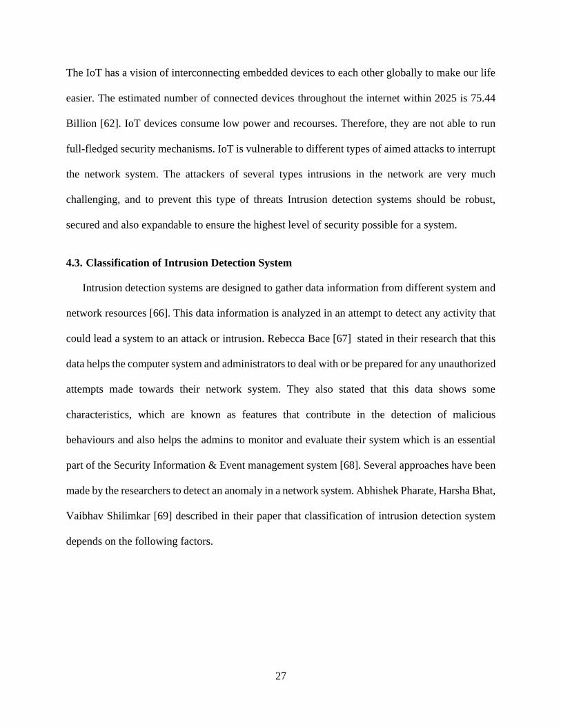
The IoT has a vision of interconnecting embedded devices to each other globally to make our life

easier. The estimated number of connected devices throughout the internet within 2025 is 75.44

Billion [62]. IoT devices consume low power and recourses. Therefore, they are not able to run

full-fledged security mechanisms. IoT is vulnerable to different types of aimed attacks to interrupt

the network system. The attackers of several types intrusions in the network are very much

challenging, and to prevent this type of threats Intrusion detection systems should be robust,

secured and also expandable to ensure the highest level of security possible for a system.

4.3. Classification of Intrusion Detection System

Intrusion detection systems are designed to gather data information from different system and

network resources [66]. This data information is analyzed in an attempt to detect any activity that

could lead a system to an attack or intrusion. Rebecca Bace [67] stated in their research that this

data helps the computer system and administrators to deal with or be prepared for any unauthorized

attempts made towards their network system. They also stated that this data shows some

characteristics, which are known as features that contribute in the detection of malicious

behaviours and also helps the admins to monitor and evaluate their system which is an essential

part of the Security Information & Event management system [68]. Several approaches have been

made by the researchers to detect an anomaly in a network system. Abhishek Pharate, Harsha Bhat,

Vaibhav Shilimkar [69] described in their paper that classification of intrusion detection system

depends on the following factors.

28

Figure 4.2: Factors contributing to the classification of the intrusion detection system.

4.3.1. Location of the Network System

Depending on the location of the network system infrastructure IDS is classified into two

categories

1. Host-Based Intrusion Detection System

2. Network-Based Intrusion Detection System

4.3.1.1. The Host-based intrusion detection system (HIDS)

The primary objective of a Host-based intrusion detection system is collecting information

regarding the security of a particular single system or host. This system has the capability of

monitoring & analyzing the packets, which are flowing through the internal computer or network

system and provide information from internal or external attacks on the system. These agent hosts

are referred to as sensors, which are executed on a machine that is more likely to be vulnerable to

possible intrusions.

Location of the Network SystemFunctionality of the Network

System

Deployment Approach Detection Mechanism

Factors Contributing on

Classification of IDS

29

Figure 4.3: Positioning of HIDS and NIDS on a netowrk

As shown in Figure 4.3, sensors in a HIDS system (installed on an individual host) collects

information about different events that take place on the system, and these events are logged by an

operational system mechanism known as audit trials [67] [66] [70]. HIDS examines specific host-

based activities such as what applications are being used, what files are being edited & what

information resides on the log file or audit trials. HIDS mostly uses anti-threat applications such

as antivirus, spyware that is previously configured on the system, which monitors security

consistently. However, HIDS is versatile, does not require bandwidth & requires less training. On

the other hand, HIDS are mostly dependent on the log’s/audit’s files, continuous log or reporting

creates an additional load to the network [69].

4.3.1.2. The Network-based intrusion detection system (NIDS)

In a network-based intrusion detection system, the system collects information directly from

the network. It monitors the network traffic continuously and analyzes the real-time traffic packets

for possible intrusions. The intrusion detection system checks for unauthorized access or abnormal

behaviour by analyzing the contents of the data packets travelling across the network. The

network-based intrusion detection systems are designed in such a way that is capable of detecting

intrusions based on intrusions specific behaviours or some known patterns called attack signatures

30

[71]. The NIDS are armed with network sensors which are generally installed on network gateways

(Please see Figure 4.3). It compares the collected data to the known attack signatures and detect

the abnormal packets if it finds a pattern match. This methodology is also known as packet sniffing

which is a detection strategy. NIDS are also ubiquitous due to their portability. They only monitor

some specific segments of a network system & independent of the operating system. NIDS are

adaptable to any network topology used and can be controlled centrally. NIDS also has some

problems to share. As it is mostly based on known attack patterns known as attack signatures, it

only can detect intrusions of known patterns. If the intrusion signatures are not on the system log,

it is unable to detect the intrusion, and the system becomes vulnerable to different attack strategies.

Another major disadvantage of the network-based intrusion detection system is encryption,

visibility & switched network. Firstly, if the packets flowing through the network is encrypted, the

sensor agents are unable to scan the contents of the packets and these packets may be ignored/

passed if there is no termination before NIDS. As most of the packets may be ignored resulting in

more false positives [72]. Secondly, due to the switched network is designed to decrease network

traffic by virtually linking two network stations & NIDS is positioned on a switched network, it

can analyze the traffic only directed towards it causing visibility issue on the overall network [67].

As a result, most of the packets, which are directed to other network segments, may deploy

intrusion, as NIDS is not monitoring them. Due to this packet loss, the accuracy and visibility both

are affected by the network intrusion detection system. Limited resources are one of the major

limitations of the network-based intrusion detection system. NIDS’s must collect, store & analyze

the captured data in real-time, but if the network load increases the sheer packets reduce the ability

of the NIDS’s to keep up with speed. NIDS’s also requires to deal with a large number of TCP

connection that requires a large amount of memory resources on the NIDS’s hosts [20].

31

4.3.2. The functionality of the Network system

Depending on the functionality IDS can be classified into two Classes

1. Intrusion Prevention System

2. Intrusion Detection & Prevention System

4.3.2.1. Intrusion Prevention System

An Intrusion Prevention System (IPS) is a network threat prevention method that inspects

the data packet flow of network packets to prevent against a security threat. The security threat is

a type of malicious activity that allows attackers to gain control of a particular application or the

whole system resulting Denial of Service (DoS) state. It can access and override all the authorized

rights or permission that compromise the network system. IPS is generally placed behind the

firewall of the detection system, which performs a series of complementary analysis for the

abnormal behaviours. The Intrusion Prevention System is implemented inline, a direct pathway

from the source to the destination and performs real-time analysis. This analysis technique is

designed to take necessary actions like sending alarms to the administrator, restricting or dropping

the malicious packets, disconnect from source to destination, master resetting the connection [72]

[73].

4.3.2.2. Intrusion Detection and Prevention System

Intrusion detection systems previously were designed only to detect malicious behaviour. Due

to the explosion of internet attacks around the globe researchers developed a system that contains

both detection and prevention system. In IDPS (Intrusion Detection & Prevention System), the

system first preprocesses the traffic data using some known data preprocessing model like linear

scaling. Then the system classifies the abnormal activities from the usual activities, therefore

prevent the malicious packet from entering or making the system vulnerable to attackers. In real

32

time data traffic sometimes the system is unable to identify all the malicious packets due to limited

resources or limited memory.

4.3.3. Deployment Approach

Depending on the factor “deployment approach” which defines where to put the detection

system on the network NIDS is divided into two more categories

1. Single Host

2. Multiple Host (Distributed Agents)

4.3.3.1. Single Host

In this deployment approach, the security system is installed on a single computer or a

device of the network system that can be a router, a network server or a network switch. All the

data traffic passed back and forth via this single host and examined for any malicious behaviour

on the network system. It is easy to implement and does not have any effect on the performance

of a network system. However, when the data traffic is very high, it becomes challenging for the

single node to process all the traffic in real time scenario.

4.3.3.2. Multiple Host

In this deployment approach, the security system is implemented on multiple computers or servers

and can be controlled centrally. Data flows through multiple nodes that reduce the workload on

the total system as data flows through multiple routes. If any activity is suspicious than it responds

immediately in real time and generate alarms to the administrator for further action. As the agent

is distributed throughout the network, all the traffic packets can be examined, and less possibility

of missing examine the packets. On the other hand, coordination between nodes requires hard

solutions [69].

33

4.3.4. Detection Method Based Classification

Depending on the detection method, the intrusion detection system is classified into two

categories.

1. Signature-Based

2. Anomaly-Based

4.3.4.1. Signature-Based Approach

A signature-based approach is made by the vendors while designing an intrusion detection

system. This signature-based mechanism protects against known threats. It can protect the system

if a malicious contents signature is known to the detection system. For example, let us say an

email contains a known malware name “Hello” which is a virus and has some patterns that are

known to the system. When a match is found in the database, an alarm is generated to the

administrator for further action or the system takes legal action according to the settings. It

implicates searching a series of bits/bytes or sequence which is termed to be malicious. This type

of signatures is easy to generate if one knows what type of network traffic is expecting. However,

this type of approach is vulnerable to unknown threats that’s signature is not recognized by the

security system. To detect an attack the signature has to be precise. Otherwise, the attacker can

modify the signatures, which are unknown to the system, and the system will allow this packet

as this modified pattern is not in its database. Therefore, signatures need to be updated on a

regular basis provided by vendors like MacAfee, Symantec and Kaspersky.

34

Figure 4.4: General flowchart of the signature-based intrusion detection method.

If not updated regularly, the system will allow packets that contain malicious data and will be

unable to protect the system. One of the critical disadvantages is signature-based approach effects

the performance of the whole system as it always tries to find a match from the database and the

database increases every moment as new signatures are generated. Another major disadvantage is

a valid signature needs to be generated for each of the attacks, and they can identify only those

attacks. They are not capable of detecting other novel attacks as their signatures are unidentified

to the detection method [74] [75] [76].

4.3.4.2. Anomaly-Based Approach

Anomaly-based network intrusion detection system is the most common mechanism

nowadays for network intrusion detection and prevention. The anomaly-based mechanism is

designed based on the concept of monitoring the data traffic flows (incoming and outgoing) on the

network system. The anomaly-based approach uses some statistical method to compare the

behaviour of the network system at one instant against a standard behaviour profile. If there is a

divergence from the normal behaviour and it surpasses a certain threshold the system generates an

alarm to notify the admin about this scenario. It is a practical approach against unknown pattern

attacks for which the system does not have pre-saved signatures. In a real-time scenario, if the

35

behaviour of the network changes or deviates from the normal behaviour, it considers it as an

intrusion. In the construction of standard behaviour profile, artificial intelligence and machine

learning techniques are considered.

Figure 4.5: General flowchart of anomaly-based detection approach.

Figure 4.5 represents a general flowchart of an anomaly-based detection system. Data flowing

from the internet is gathered using different tools such as Mozenda, Connotate, import.io,

Wireshark and Microsoft message analyzer. These gather raw data needs to be preprocessed using

some statistical preprocessing method (statistical method selected by the designer). It is important

to pre-process the raw data samples, as these samples will be given as an input to different

anomaly-based detection method. From this pre-processed data sample or max, a portion is passed

through the anomaly detection method used for the detection scheme. The detection method deeply

analyzes the data samples and try to differentiate between normal and abnormal activity. For

differentiating between normal and abnormal behaviours, there are several methods or machine

learning application such as a support vector machine [77], artificial neural network [78], decision

trees [40]. If any malicious behaviour is matched with known patterns or reference data the system

generates an alarm to the administrator and suggests some necessary actions needs to be taken.

36

The human analyst deeply analyzes the cause of the alarm and take necessary steps based on the

data provided by the alarm. The human analyst also updates the reference data. Updating the

reference data is essential as the system is designed to learn from the day-to-day activities and

gather more information to provide a secure system.

37

Chapter 5

5. Dataset and attack types

The first dataset used in this research were taken from the Cyber Range Lab of the Australian

Centre for Cyber Security (ACCS) [19]. In this dataset, a hybrid of real modern normal

activities and attack behaviours were generated. This dataset contains total forty-seven features

and contains around 2.5 million sample data [19] [20]. It consists of such type of attacks like

Fuzzers, Analysis, Backdoors, DDoS, Exploits, Generic, Reconnaissance, Shellcode, Worms

& normal data samples with labels.

In the UNSW dataset, 47 columns represent attributes/features. Each recorded sample consists

of attributes of different data forms like binary, float, integer and nominal. The attack data

samples are labelled as ‘1,’ and normal data samples are labelled as ‘0’. Some of the feature

data sample values are categorical values. For example, source IP address, destination IP

address and source port number. Also, some other feature data sample values are continuous

variable. For example, source bits per second, source jitter, and source TCP windows

advertisement value. For preprocessing purpose, the features which values are categorical values

were assigned a key value and stored in a dictionary. In the dictionary object, any values can be

stored in an array, and each recorded item is associated with the form of key-value pairs.

Furthermore, all the data samples were normalized using the following normal feature scaling

process:

𝑋′ =𝑥 − min (𝑥)

max(𝑥) − min (𝑥) (16)

38

where 𝑋′ is the normalized value and 𝑥 is the original value. The file was saved into a .txt file for

SVM input. In this way, all the data samples were preprocessed in the same pattern.

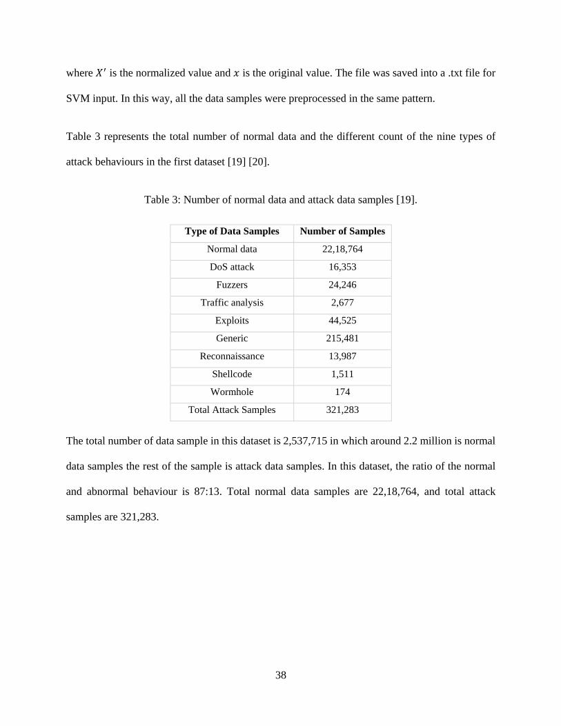
Table 3 represents the total number of normal data and the different count of the nine types of

attack behaviours in the first dataset [19] [20].

Table 3: Number of normal data and attack data samples [19].

Type of Data Samples Number of Samples

Normal data 22,18,764

DoS attack 16,353

Fuzzers 24,246

Traffic analysis 2,677

Exploits 44,525

Generic 215,481

Reconnaissance 13,987

Shellcode 1,511

Wormhole 174

Total Attack Samples 321,283

The total number of data sample in this dataset is 2,537,715 in which around 2.2 million is normal

data samples the rest of the sample is attack data samples. In this dataset, the ratio of the normal

and abnormal behaviour is 87:13. Total normal data samples are 22,18,764, and total attack

samples are 321,283.

39

The second dataset used in this research paper was collected from Canadian Institute of Cyber

Security Excellence at the University of New Brunswick [21] upon request. The dataset is named

as CIC IDS 2017, which is an Intrusion detection and evaluation dataset specially designed by

collecting real-time traffic data flows over seven days that contains malicious and normal

behaviours. In this dataset, there are over 2.3 million data samples, and among them, only 10%

represents attack data samples. There are 80 network flow features in this data set. The traffic data

samples contain eight types of attacks namely Brute Force FTP, Brute Force SSH, DoS,

Heartbleed, Web attack, Infiltration & DDoS [21]. This dataset is one of the richest datasets used

for Network intrusion detection research purposes around the world [24]. The goal of using this

data set is to evaluate how the proposed method works on different datasets.

5.1. Types of Attack

Several types of attacks occur in the network. They are mainly classified into two types [79].

5.1.1. Active Attack

An active attack in the network system, the hacker (attacker) attempts to enter and malfunction

the system, by affecting their proper regular operation. Active attacks always cause severe damage

to the system, and the victim receives intruder alert. It is a severe threat to integrity and availability,

which is an essential requirement for a secured network system. Some active attacks are described

below:

I. Spoofing

A spoofing attack is a malicious practice in which the intruder falsifies its identity to access

the system and gain illegitimate advantages over the system. In a spoofing attack,

communication is initiated by the attacker to the victim from an unknown source, but it

40

pretends to present itself as an authentic and safe sender. Spoofing attacks are generally

used to spread malware and to access confidential information [80].

II. Wormhole

Wormhole attack is a severe type of network intrusion in the Wireless network system. It

is also referred to as tunnelling attack. In this attack, the attacker receives a data packet and

creates a shorter passageway (tunnels) to another malicious node of the network. It shows

that the packet found a shorter path from the source to destination [81].

III. Modification

Modification refers to modifying the contents or the route of the packet flow on the network

system. As a malicious node modifies the traffic route, it creates communication delay

between the sender and the receiver [82].

IV. Denial of Service

Denial of service (DoS) attack is a severe threat to the network system. This attack occurs

when a malicious user/node tries to send data, and it consumes much bandwidth of the total

system. The resources become low, and the traffic load gets higher in volume. Then it

makes the network service unavailable to the user, affecting the availability of the system,

which is one of the significant requirements of an efficient & secure system [83].

V. Sinkhole

The sinkhole is a type of network attack which aim is to prevent the receiver from receiving

correct and accurate information in the packet. If a node is compromised, then it tries to

spread to the different nodes are trying to alter the data packets that result in some delay

41

on the network traffic, and the correct content is not received at the receiver end. The data

that the receiver will receive may contain unwanted applications or Trojans [81].

VI. Shellcode

Shellcode is a type of some small program or code that the attacker implement on a network

node, allows the attacker to take control of that particular node and spread throw-out the

system. Shellcode can be either remote or local, depends on the weather it gives an attacker

the control of the machine or control over another machine form a remote location [84].

5.2. Passive Attack

The primary function of passive attack is it intends to read or make use of the information it's

monitoring without authorization, but does not influence the resources of the system. It refers to a

type of attack that is in the system and continuously monitoring the data packets as an intruder. It

is a severe threat to the confidentiality of the network system. It can get access to some classified

information, which has been sent and received by the authorized user, and the attacker can see the

contents and collect information. The victim is unaware of the scenario as it quietly monitors the

system. The system needs to have some countermeasures to prevent this type of network attacks.

Some active attacks are described below:

I. Monitoring

This type of attacks silently monitors the traffic flow on the network from the source to the

destination path. It does not make any changes but keeps an eye on the information

transmitted [79].

42

II. Traffic Analysis

In this type of attack, the attacker analyzes the data travelling from source to destination.

It gathers all the volume of data travelling from and to the route. It does not make any

modification of the contents.

III. Eavesdropping

Eavesdropping is a type of attack that often occurs in the mobile ad-hoc networks. The

primary approach of the attack is to continuously search for confidential information over

the data flow [79].

43

Chapter 6

6. Proposed Algorithm

In this chapter, the proposed algorithm is explained. The first algorithm represents an initial

approach to the research. Since then, several changes have been made to overcome some major

limitations.

6.1. Initial Algorithm [85]

1. Define the number of features,𝐾 from the dataset.

2. Select 𝑛 features among 𝐾 features using a random combination.

3. Run SVM for 𝐾 featured training examples

a) Select the total number of N data samples (n featured) to run the SVM.

b) Select the SVM parameter (Gamma, coef 𝜃, nu)

c) Select 𝐾 × 𝑁 data sample for training and save the data on 𝑇𝑡𝑟𝑎𝑖𝑛 dataset

d) Select 𝑛 × 𝑀 data samples for testing and save it in 𝑇𝑡𝑒𝑠𝑡 dataset

e) Using 𝑇𝑡𝑟𝑎𝑖𝑛 train the SVM

f) After training, the learning performance of SVM is evaluated. Using 𝑇𝑡𝑒𝑠𝑡, detection

accuracy, false positive rate, false negative rate and time taken to run the model are

measured.

4. Repeat the procedure from 1-3 until we achieve the highest detection accuracy, low false

positive and false negative rate.

At first, the proposed scheme defines the number of features in the data set. Furthermore, n features

are selected using random permutation to see which combination of the features are relevant to

achieve a reasonable detection accuracy. After that, the algorithm selects the N number of data

samples, which contains both normal and abnormal data traffic pattern to run the SVM based

scheme. Then it randomly selects n number of appropriate features for detecting abnormal

behaviour from network data traffic. Before running the algorithm, we set parameters of the

proposed algorithm such as gamma, coef 𝜃 and nu. After mixing up the dataset, 𝐾 × 𝑁 data

samples are selected so that the SVM can learn the dataset without any bias. These samples are

stored in Ttrain that will be used for training purpose. Similarly, 𝑛 × 𝑀 data samples are chosen and

44

stored in Ttest to verify the learning performance of the SVM based detection scheme. After

performing the learning procedure of SVM, detection accuracy, false positive rate and time to run

the algorithm are measured. Furthermore, the number of detection features are increased and the

whole process is repeated from 1-3 [85].

6.2. Proposed Algorithm [86]

1. Define the number of features, N from the feature space

2. Select the SVM parameter (Gamma, coef (), nu)

3. Define Number of Cooling (nCL) and Equilibrium loop (nEL)

4. Cooling loop Starts {i=1 to nCL}

a) Select n features from 𝑁, where 𝑛 ∈ 𝑁

b) Define an array DR_array of size 10

5. Equilibrium-loop starts {𝑗=1 to nEL}

a) Train the SVM with the only 𝑛 selected feature

b) Test the learning performance of SVM

c) Store the solution in DL

d) A small random perturbation of the features

e) Repeat step 5a & 5b

f) Save the Solution in DR

g) DR_array [𝑗 %10] = DR

6. if 𝑗 ≥10 and Standard Deviation (DR_array) ≤ √2

a) Break from Equilibrium and Continue to Cooling loop

7. If DR > DL, then DL DR

8. Else

a) Find the Probability of Acceptance P

b) Generate Random Number R

c) If P > R, DL DR

d) If P < R, Check if number of Equilibrium loop (nEL)==0

e) If (nEL)! =0, repeat 5(d), 5(e), 5(f)

f) Else If (nEL)==0, Then DL DR

9. Else If (nEL)==0, Reduce Temperature.

10. Equilibrium Loop Ends

11. Check Number of cooling loop (nCL)==0?

12. If (nCL)==0, Done

12. Else repeat procedure 4

45

The proposed scheme defines the number of features in the dataset. Furthermore, the SVM

parameters (Gamma, coef (), nu), Number of cooling loops (nCL), Number of equilibrium loops

(nEL) are defined. At first, in the cooling loop, 𝑛 number of features among 𝑁 features are

randomly selected (as initially, it does not know where to start with) where 𝑛 ∈ 𝑁. Then it moves

inside the equilibrium loop, and trains the SVM only with the selected 𝑛 number of features and test

the learning performance of SVM. Then the algorithm saves the solution in DL. This solution is

considered as an initial solution, and the goal of this loop is to find a best solution for the given

temperature. A small random perturbation of the currently held features is made (seems like a

random walk in the feature space) to create a new possible solution because it is believed that

good solution is generally close to each other but it is not guaranteed. The algorithm stores the

solution in DR. If the cost of the new candidate solution is lower than the cost of the previous

solution, then the new solution is kept and replaces the previous solution. Also, if the solution

remains within ±2% and factored by ten times in a row, the algorithm will terminate the current

equilibrium loop and will check the cooling loop (if nCL≠ 0) and continue another equilibrium

loop to save time as its trapped in that local optimum solution. Sometime the random perturbation

results in worse solution then the algorithm decides to keep or discard the solution, which

depends on an evaluation of the probability function. In a case that the new solution is worse than

the previous one then, the algorithm generates a random number R and compares with the

probability function. If 𝑃 > 𝑅, the algorithm keeps the worse solution and if 𝑃 < 𝑅, then the

algorithm checks whether it has reached the defined number of equilibrium loops or not. If

(nEL)==0 then it moves out from the equilibrium loop to cooling loop and restarts the above

described procedure again from the cooling loop. If (nEL)! =0, then the algorithm starts from

random perturbation inside the equilibrium loop and performs the procedure again. When the

46

number of cooling loop reaches zero, then algorithm terminates and provide a meaningful

solution [86]. This procedure is consuming less time and does not need and specific hardware

configuration.

This algorithm does not search the whole work/feature-space for reaching the global optimum

solution. As a result, a small amount of time is required to provide a reasonable solution. It

performed relatively well in large datasets. The efficacy of the proposed solution depends on the

selection of essential features that help the intrusion detection process to detect an anomaly

accurately. To assure that the algorithm provides a better solution compared to other machine

learning methods, it has been tested on two different type of datasets, which was explained in the

previous chapter.

47

Chapter 7

7. Experiments and Results

This chapter is divided into several sections. In the first section, simulation setup and outputs

using the initial algorithm have been discussed in details. The second section will highlight the

outputs using the proposed algorithm. Both the dataset contains different numbers of features. The

results are discussed in details using multiple feature subsets (Ex. 2, 3, 4 and 5).

7.1. Simulation Setup for General SVM based detection method

In this setup, a total number of features were 47 and the algorithm randomly selected three features

at a time. The total number of samples was around 2.5 million, in which 2,032,034 samples were

taken for training purpose of the algorithm and rest 5,080,10 samples for the testing purpose. The

following Table 5 represents a subset of the combinations of the features taking three at a time.

Further, this table provides detailed information what does each combination number represents.

For example, combination number 1 represents a feature set of Source IP address, the TCP

sequence number of the destination and the number of connections in the same source and

destination tuple.

48

Table 4: Simulation setup parameters (3-features for the initial algorithm).

Parameter Value

Total number of samples 2540044

Number of features 47

Number of features selected 3

Training data samples 2032034

Testing data samples 508010

Table 5: 3-Feature combinations subsets.

Combination

Number

Features in this Combination [19] [20]

1 a. The IP address of Source

b. TCP based sequence number of the destination

c. Number of connections is same source address & the destination port in 100 connections

according to the uncompressed content size of data transferred from the HTTP service

2 a. Source TCP window advertisement value

b. Source Jitter (mSec)



3 a. Source TCP based sequence Number

b. Destination TCP Window Advertisement value



4 a. Destination TCP based sequence Number

b. Source TCP based sequence Number

c. Mean value of the flow packet size transmitted by the Destination

5 a. Actual uncompressed content size of data transferred from the HTTP service

b. Destination Jitter

c. Number of connections is the same destination address & the source port in 100

connections according to the uncompressed content size of data transferred from the HTTP

service 6 a. Source Jitter (mSec)

b. Source retransmitted packet

c. Source TCP window advertisement value

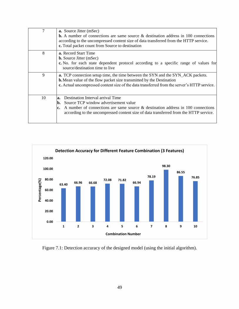
49

7 a. Source Jitter (mSec)

b. A number of connections are same source & destination address in 100 connections

according to the uncompressed content size of data transferred from the HTTP service.

c. Total packet count from Source to destination

8 a. Record Start Time

b. Source Jitter (mSec)

c. No. for each state dependent protocol according to a specific range of values for

source/destination time to live

9 a. TCP connection setup time, the time between the SYN and the SYN_ACK packets.

b. Mean value of the flow packet size transmitted by the Destination

c. Actual uncompressed content size of the data transferred from the server’s HTTP service.

10

a. Destination Interval arrival Time

b. Source TCP window advertisement value

c. A number of connections are same source & destination address in 100 connections

according to the uncompressed content size of data transferred from the HTTP service.

Figure 7.1: Detection accuracy of the designed model (using the initial algorithm).

63.4066.96 66.68

72.08 71.8266.94

78.19

98.30

86.55

76.85

0.00

20.00

40.00

60.00

80.00

100.00

120.00

1 2 3 4 5 6 7 8 9 10

Pe

rce

nta

ge(%

)

Combination Number

Detection Accuracy for Different Feature Combination (3 Features)

50

Figure 7.1 gives the detection accuracy of the proposed method according to the feature

combination. In Table 5, the combination number denotes which three features were selected

for that combination. The proposed algorithm achieved a detection accuracy recorded as

98.30% when combination number 8 was selected (Table 5). This combination contains three

essential features such as Source interpacket record time, Source jitter and No. for each state

dependent protocol according to a specific range of values for source/destination time to live

value. The lowest detection accuracy among the given results was recorded as 63.40% for

combination number 1.

Figure 7.2: False positive & false negative rate.

28.9630.73 31.00

16.33

25.87

0.40

9.55

1.61 0.81

20.82

7.64

2.31 2.31

11.60

2.31 2.25

12.26

0.17

12.64

2.33

0.00

5.00

10.00

15.00

20.00

25.00

30.00

35.00

1 2 3 4 5 6 7 8 9 10

Pe

rce

nta

ge (

%)

Combination Number

False positive and False Negative rate for different feature combination

False Positive False Negative

51

Furthermore, the performance metrics of the proposed algorithm was investigated. The false

positive refers to a situation that the system incorrectly identifies an object as a positive

(attack), which, however, is not an attack and is a normal (non-attack) object. Figure 7.2

represents the percentage of the false positive and false negative rate for the proposed scheme.

The lowest false positive and false negative rate were recorded as 1.61% and 0.17%

respectively while combination number 8 was considered. It is evident that if all the possible

combinations are tried out, the best result can be shown although it is keeping us to the

exhaustive search problem.

Figure 7.3: Receiver operating characteristic curve of the designed model.

In Figure 7.3, the Receiver operating characteristic curve is presented which is a graphical plot

that demonstrates the analytical ability of the binary classifier system at various thresholds. It is

implemented by plotting the True positive rate (Y-axis) against the false positive rate (X-axis).

52

From the graph, we can visualize that combination number 8 is better than any other possible

solutions generated by the algorithm. The area under the curve (in ROC) is a statistical measure of

the accuracy of a quantitative test. The accuracy of the test depends on how well the test separates

the positive and negative data samples. An AUC value of 1 represents a perfect solution, and an

area of 0.5 represents a worse solution.

AUC is classification-threshold-invariant; implying that it measures the quality of the model's

predictions regardless of what classification threshold is selected. We can see the AUC (area under

the curve) value 0.98815 for the combination number 8, which is closer to one in contrast to the

other combinations. The lower AUC value was recorded as 0.44743 when the algorithm

considered combination number 4.

The limitations of this algorithm are it is searching the whole workspace and trying all possible

feature combinations (16,215 combinations when taking three at a time according to equation 2)

which leads to an exhaustive search problem which takes a huge amount of time. If the dataset is

big enough, and we try more number of feature combination like taking 3, 4, 5 or more at a time

the algorithm will try all (for four features 1,78,365, for five features 1,533,939, for six features

1,073,7,573) combinations according to equation (1) to provide the best reasonable output. In this

scenario, the exhaustive search exists and leading to a combinatorial optimization problem. It may

take eons to provide a solution using a large number of features in big data analysis.

53

7.2. Simulation Setup for Proposed Algorithm (2 features)

Table 6: Simulation setup parameters (2-features for the updated proposed algorithm).

Parameter Value






In this simulation setup, the proposed algorithm has been applied taking two feature subset as an

initial approach. Afterwards, we will try three, four and five feature subset combinations to inspect

how the algorithm performs if the number of features increases in a subset. Table 7 refers 2-feature

subset combinations:

Table 7: 2-feature subset combinations

Combination

Number


1

a. a. The IP address of Source

b. b. Service used (HTTP, FTP, SMTP, ssh, DNS, FTP-data, IRC and (-) if not much-

used service)

2

a. No of connections of the same source IP and the destination IP address in 100

connections according to the uncompressed content size of data transferred from the

HTTP service last time

b. Destination interpacket arrival time (mSec)

3 a. Source TCP based sequence Number

b. Some flows that have methods such as Get and Post in HTTP service.

4

a. Destination TCP based sequence Number

b. Mean value of the flow packet size transmitted by the Destination

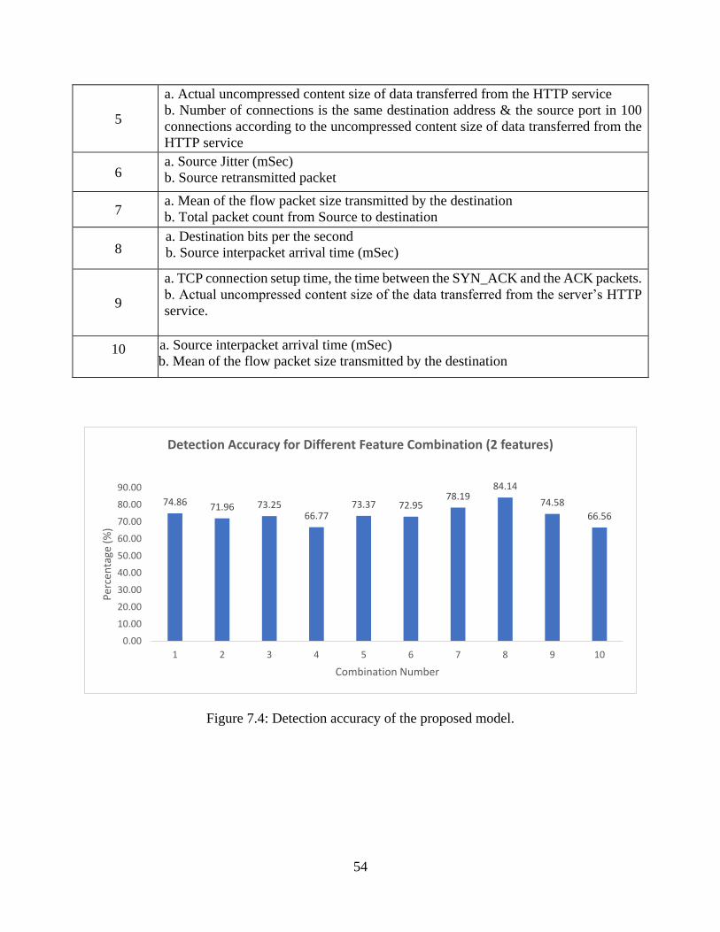
54

5

a. Actual uncompressed content size of data transferred from the HTTP service

b. Number of connections is the same destination address & the source port in 100


HTTP service

6 a. Source Jitter (mSec)


7 a. Mean of the flow packet size transmitted by the destination

b. Total packet count from Source to destination

8 a. Destination bits per the second

b. Source interpacket arrival time (mSec)

9

a. TCP connection setup time, the time between the SYN_ACK and the ACK packets.

b. Actual uncompressed content size of the data transferred from the server’s HTTP

service.

10

a. Source interpacket arrival time (mSec)

b. Mean of the flow packet size transmitted by the destination

Figure 7.4: Detection accuracy of the proposed model.

74.86 71.96 73.2566.77

73.37 72.9578.19

84.14

74.58

66.56

0.00

10.00

20.00

30.00

40.00

50.00

60.00

70.00

80.00

90.00

1 2 3 4 5 6 7 8 9 10

Per

cen

tage

(%

)

Combination Number

Detection Accuracy for Different Feature Combination (2 features)

55

Figure 7.5: False positive & false negative rate.

Figure 7.6: Receiver operating characteristic curve.

23.06

17.8415.64

30.96

14.04

0.40

9.55

5.09

20.40

31.12

2.08

10.20 11.11

2.27

12.59

4.31

12.2610.77

5.022.32

0.00

5.00

10.00

15.00

20.00

25.00

30.00

35.00

1 2 3 4 5 6 7 8 9 10

Per

cen

tage

(%

)

Combination Number



56

Figure 7.7: F1 score of the detection scheme.

The F1 score is a statistical analysis of binary classification and a measure of tests precision.

The F1 score can be described as a harmonic mean of the precision and recall, where an F1

score reaches its best value at one and worse at 0. Precision is the ratio of correctly projected

positive annotations to the total projected positive annotations whereas recall is the ratio of

correctly predicted positive annotations to the all annotations in the actual class. The reason

why harmonic mean is considered as the average of ratios or percentages is considered. In this

case, harmonic mean is more appropriate then the arithmetic mean. The F1 score of the

combinations where two features were taken at a time does not seem quite good enough.

Evaluating the above results, it has been seen that the algorithm was able to provide a detection

accuracy of 84.14% (combination number 8).

57

Considering only two feature subsets provided a high false positive and false negative rate of

5.09% and 10.77% respectively. Upon checking the ROC curve, these combinations provided

poor AUC value. It may be caused by taking an imbalanced number of features. The feature

subset is selected by the SA process which may not be linearly separable on the classification

space. Using a non-linear typical decision boundary will require more computational efforts than

fitting linear decision boundary. Thus, increasing the dimension (or features) may provide better

results compared to the 2-feature subsets as it may allow the hyperplane to separate the data.

7.3. Simulation Setup for The Proposed Algorithm (3 features)

Table 8: Simulation setup parameters (3-features for the proposed method).

Parameter Value






In this simulation setup, a 3-feature subset was considered to analyze the performance of the

proposed algorithm. The number of training and testing data samples were kept the same as

previous. The performance was inspected by evaluating the performance metrics; detection

accuracy, false positive, false negative, Area under Curve value and F1 score. The simulation

outcomes were compared with 2-feature subset combination results. Furthermore, the outcomes

were also analyzed in depth in comparison with general SVM based detection method.

58

Table 9: Feature combination (3-feature for the proposed method).

Combination

Number


1

c. a. The IP address of Source

d. b. Service used (HTTP, FTP, SMTP, ssh, DNS, FTP-data, IRC and (-) if not much-

used service)

e. c. Source packets retransmitted or dropped

2

a. Source TCP window advertisement value

b. No of connections of the same source IP and the destination IP address in 100


HTTP service last time

c. Destination interpacket arrival time (mSec)

3

a. Source TCP based sequence Number

b. Some flows that have methods such as Get and Post in HTTP service.

c. No. of connections of the same destination address in 100 connections according

to the uncompressed content size of data transferred from the HTTP service last time

4

a. Destination TCP based sequence Number

b. Source TCP based sequence Number

c. Mean value of the flow packet size transmitted by the Destination

5

a. Actual uncompressed content size of data transferred from the HTTP service

b. TCP base sequence number of destinations

c. Number of connections is the same destination address & the source port in 100


HTTP service

6

a. Source Jitter (mSec)


c. Destination bits per second

7

a. Source Jitter (mSec)


c. Total packet count from Source to destination

8

a. Destination bits per the second


c. No. for each state dependent protocol according to a specific range of values for

source/destination time to live

9

a. TCP connection setup time, the time between the SYN_ACK and the ACK packets.

b. Source bits per second

c. Actual uncompressed content size of the data transferred from the server’s HTTP

service.

10

a. Destination Interval arrival Time


c. Mean of the flow packet size transmitted by the destination

59

As shown in Table 9, a list of ten combinations has been shown, and each combination contains

three features. The mechanism of the initial approach was that it takes three features at a time

and provide an output. Afterwards, it discards the results and tries another randomly selected

feature combination. Trying all possible combination implies that it leads to an exhaustive search

and takes a huge amount of computational resources and consumes more time. Further, it will

more time if a large number of features are considered. However, in the proposed algorithm, the

annealing process starts selecting a random set of three features as the first step as it has to begin

somewhere randomly. Then the SVM is trained only with these three features, and the generated

output is saved. It is considered as a first initial solution. A small random perturbation is made

to the current solution changing one or two features because it is assumed that good solutions

are generally close to each other, but it is not guaranteed as the best solution. Sometimes the

newly generated solution results in a better solution than the algorithm keeps the new solution.

If the newly generated solution is worse than the current solution, then the algorithm decides

whether to keep or discard the worse solution, which depends on the evaluation of the

probability function (Equation 11). The higher temperature in the annealing process, it is more

likely the algorithm will keep the worse solution. Keeping the worse solution allows the

algorithm to explore the solution space and to keep it within the local optima. Also neglecting a

worse solution lets the algorithm to exploit a local optimum solution, which could be the global

solution for that temperature.

The outputs of the proposed algorithm are provided and discussed in details in contrast with the

general SVM alone based approach.

60

Figure 7.8: Detection accuracy of the proposed scheme.

Figure 7.8 shows the detection accuracy of the proposed method according to the feature

combination. In Table 9, the combination number denotes which three features were extracted

for that combination. The proposed algorithm achieved a detection accuracy recorded as 98.32%

when combination number 8 was selected (Table 9). This combination contains three essential

features such as destination bits per second, source interpacket arrival time (mSec), Number of

each state dependent protocol according to a specific range of values for source/destination time

to live value. The lowest detection accuracy among the given results was recorded as 72.08%

when combination number 4 was considered. Comparing with the 2-feature subset combination

results, we can infer that as another dimension was introduced, the linear classification technique

worked better.

73.0876.83 77.14

72.0877.55

82.5386.58

98.32

87.33 86.38

0.00

20.00

40.00

60.00

80.00

100.00

120.00

1 2 3 4 5 6 7 8 9 10

Pe

rce

nta

ge(%

)

Combination Number

Detection Accuracy for Different Feature Combination (3 Features)

61

Figure 7.9: False positive and false negative rate of the proposed scheme.

Furthermore, the performance metrics of the proposed algorithm was investigated. The false

positive refers to a situation that the system incorrectly identifies an object as a positive

(attack), which, however, is not an attack and is a normal (non-attack) object. The false

negative refers to a situation that the system incorrectly identifies an object as a negative

(non-attack), which however is an attack. In Figure 7.9, the percentage of false positives and

the percentage of false negatives are shown for the proposed scheme. The false positives and

false negatives were recorded as 1.49% and 0.19% respectively while combination number

8 was considered. Therefore, it can be inferred that if the correlative features are extracted the

false positive and negative rate decreases, it may provide a relatively better solution for

intrusion detection.

22.5620.83

17.2616.33

18.27

0.40 0.82 1.490.01

0.99

4.36

2.34

5.60

11.60

4.18

0.81

12.60

0.19

12.66 12.62

0.00

5.00

10.00

15.00

20.00

25.00

1 2 3 4 5 6 7 8 9 10

Pe

rce

nta

ge (

%)

Combination Number



62

Figure 7.10: Receiver operating characteristic curve.

In Figure 7.10, the receiver operating characteristic curves for the proposed schemes are presented.

In a real-world scenario, the misclassifications costs are difficult to determine. In this regard, the

ROC curve and its related measures such as AUC (Area under Curve) can be more meaningful

and vital performance measures. As shown in Figure 7.10, it is seen that the performance output

is much better than the previous performance of the algorithm. The combination number 8 which

contains features such as Destination bits per second, Source interpacket arrival time (mSec),

Number of each state dependent protocol according to a specific range of values for

source/destination time to live value, provided much better reasonable output. The AUC of that

63

combination is 0.98384, which is closer to one, which presents a better solution in contrast with

the other possible solutions.

Figure 7.11: F1 score of the proposed method.

Once a model has proposed it is very important that how much good is the model. The performance

of the model can be measured using a different type of statistical measure. The F1 score is a

statistical analysis of binary classification and a measure of tests accuracy. The F1 score can be

interpreted as a harmonic mean of the precision and recall, where an F1 score reaches its best value

at 1 and worst at 0. Precision is the ratio of correctly predicted positive annotations to the total

predicted positive annotations whereas recall is the ratio of correctly predicted positive

annotations to the all annotations in the actual class. The reason why harmonic mean is considered

as the average of ratios or percentages is considered. In this case, harmonic mean is more

appropriate than the arithmetic mean. F1 score proves to be a more realistic measure of the

64

classifier performance. The above graph shows the F1 score of the different combinations and

combination number 8 achieved the highest F1 score of 0.9905 which is closer to 1 in contrast to

the other combinations.

Figure 7.12: Detection accuracy difference with the increasing number of iterations.

Figure 7.12 demonstrates the detection accuracy of the proposed scheme increases or decreases

along with the number of iterations keeps moving forward. Cross-validation mechanism is used to

assess the predictive performance of the model to evaluate how good the model works on a new

independent dataset (using resampling randomly). In Figure 7.12, it is seen that combination 1

(violet) started with very low detection accuracy, but while iterating multiple times the detection

accuracy increased, and an average of those accuracies provide a well reasonable solution for that

combination.

On the other hand, combination 8 (light brown) started with higher accuracy, and while multiple

iterations are running, it kept almost the same as it is and an average of those accuracies has been

considered. Furthermore, the combination number 4 (sky blue) stared with higher accuracy but

while multiple times iterations the accuracy went down and suddenly went up. An average of those

65

accuracies has been considered. Taking averages of the detection accuracies allows the algorithm

to be more confident on the provided output. The proposed scheme does not take too long to

converge to the local optima (which can be the global optima) but provides a reasonable detection

accuracy over short possible time depending on the system resources.

Figure 7.13: Performance of the proposed scheme inside equilibrium loop.

To evaluate whether the algorithm works the way it supposes to work, a sum of equilibrium loops

is visualized on the above Figure 7.13. The annealing process starts at a random direction as it

does not know which direction to start with and the first solution is considered as the initial

solution. Afterwards, a random perturbation in the solution space has been performed, and a new

66

solution is generated. Comparing with the previous solution it is better or worse, it keeps the better

solution and marches forward, as it is believed the good solutions may be nearby. On the above

Figure 7.13, it is visualized that the algorithm started with a low detection accuracy and marching

forward it is going towards higher accuracy. While going forward, it seems that it may have found

worse candidate solution (the down hikes on the Figure 7.13), but keeping the worse solution

allows the algorithm to explore more in the solution space for reach an optimum solution. It proves

that the algorithm is performing the way it supposes to perform.

Figure 7.14: Detection accuracy of the equilibrium loops.

67

As the algorithm starts from a random direction, provides an initial solution, takes random

perturbation, and generates another new solution, a scenario is visualized that sometimes the

detection accuracy of the old candidate solution and new candidate solution is quite close enough

like a slight difference of some percentage. For the time being, it is being trapped on that local

optima. So, to save more time and speed up, the algorithm is designed in such way that, if the

difference of the accuracy of the old candidate solution and new candidate solution is around ±2%

and ten times in a row, the algorithm will terminate that equilibrium loop. Subsequently, the

algorithm will go to the next cooling loop (if nCL! =0) and start another inner loop and continue.

On the above Figure 7.14, inside the equilibrium loop iteration number approximately from 139-

150, the detection accuracy stays between 86%-87% for the time being, and it detected an accuracy

difference of ±2% ten times in a row. Therefore, the proposed method will terminate the current

equilibrium loop, decrease temperature and start the next cooling loop if nCL! =0.

In Table 5 and Table 9, ten combinations (each combination has three features) has been

analyzed, and the results are demonstrated. The initial algorithm extracted the features in the

combinations in Table 5 and the combinations in Table 9, were extracted by the proposed

method. We can see that in the Table 5 combination number 8, which contains three features

such as Record Start Time, Source Jitter (mSec) and the number for each state dependent

protocol according to a specific range of source/destination time to live value provides the

accuracy of 98.30%. The false positives and false negatives were recorded as 1.61% and 0.17%

respectively. On the other hand, the proposed algorithm provided a higher accuracy of 98.32%,

a lower false positive and false negative rate of 1.49% and 0.19% respectively in comparison

with the general SVM based method using features such as Destination bits per second, Source

interpacket arrival time (mSec) and Number of each state dependent protocol according to

68

specific range of values for source/destination time to live value. The proposed algorithm uses

the set of features either together or in separate depending on the perturbation factor (change one

or two features) and provide a solution which may or may not be optimal. The algorithm

subsequently decides whether to keep the new solution or not, depending on the comparison with

previously selected features and the results, whereas the initial approach discards all the features

that were previously taken and keeps searching randomly in the feature space. Therefore, this

algorithm is optimum in selecting good features incrementally. However, if the new selection is

better from the previous ones, then it discards the previously selected features. The exhaustive

search mechanism from the initial approach tries all possible combinations, whereas the

proposed scheme does not need to try all the combinations but provides a reasonable solution

compared to general SVM based solution, which may be the global optimum solution or if not,

then it will be a better sub/near-optimal solution.

In a nutshell, the proposed algorithm starts from a random path to find an initial solution (initial

3 feature combination) and takes small random walk in the feature space (changing 1 or more

features) and compares with the previous solution that allows the algorithm to converge faster to

the local optima which may be the global optimum solution. Furthermore, the performance of

the algorithm was evaluated taking four and five features in a subset.

69


In this setup, the four-feature combination was considered, and the performance was evaluated

regarding detection accuracy, false positive and negative, F1 score, ROC characteristics, Area

under the curve.

Table 10: Simulation setup parameters (4-feature subset).

Parameter Value






The algorithm will initiate with a four-feature subset combination. Furthermore, the outcomes with

bee compared with the 3-feature subset combinations. The comparision allows us to determine

how the algorithm performs when the number of features increases. The number of training

samples and the number of testing samples were kept the same as previous. In Table 11 below the

combination of four features are shown:

70

Table 11: Four-feature subset combinations.

Combination

Number

Features Taken [19] [20]

1 a. Source IP address

b. Source packets retransmitted or dropped

c. Destination to the source packet count

d. No of connections of the same source address (1) and the destination port (4) in 100

connections according to the last time (26).

2 a. Source inter-packet arrival time (mSec)

b. Destination inter-packet arrival time (mSec)

c. If the FTP session is accessed by user and password then 1 else 0.

d. No. of connections that contain the same service (14) and source address (1) in 100 connections

according to the last time (26)

3 a. Source to destination time to live value

b. Source TCP sequence number

c. No. of flows that has methods such as Get and Post in HTTP service.

d. No of flows that have a command in a n FTP session.

4 a. Destination IP address

b. Destination TCP window advertisement value

c. Source TCP sequence number

d. Mean of the flow packet size transmitted by the destination

5 a. The content size of the data transferred from the server’s HTTP service.

b. No of connections of the same destination address (3) and the source port (2) in 100 connections

according to the last time (26).

c. No. of connections that contain the same service (14) and destination address (3) in 100

connections according to the last time (26).

d. Source TCP window advertisement value

6 a. Source jitter (mSec)

b. Destination bits per second

c. No. of connections that contain the same service (14) and source address (1) in 100 connections

according to the last time (26).

d. No of flows that have a command in a n FTP session.

7 a. Source to destination packet count


c. The time between the SYN_ACK and the ACK packets of the TCP.

d. No. of flows that has methods such as Get and Post in HTTP service.

8 a. No. for each state according to a specific range of values for source/destination time to live

value

b. Destination bits per second

c. Source bits per second

d. The time between the SYN and the SYN_ACK packets of the TCP.

9 a. The content size of the data transferred from the server’s HTTP service.


c. HTTP, FTP, ssh, DNS., else (-)

d. Mean of the flow packet size transmitted by the destination

10 a. No. for each state according to a specific range of values for source/destination time to live

value


c. Destination jitter (mSec)

d. If t h e source equals to t h e destination IP addresses and port numbers are equal, this

variable takes value one else zero

71

Figure 7.15: Detection accuracy using the proposed for the four-feature combination.

Figure 7.16: False positive and negative rate.

87.57

78.2783.25

71.31

87.42 87.42 87.56

97.97

80.44

98.39

0.00

20.00

40.00

60.00

80.00

100.00

120.00

1 2 3 4 5 6 7 8 9 10

Pe

rce

nta

ge(%

)

Combination Number

Detection Accuracy of Different Feature Combinations (4 Features)

7.589.18 9.18

17.46

0.27 0.401.55 1.64

14.91

0.24

4.86

12.55

7.57

11.2312.32 12.57

10.89

0.39

4.64

1.37

0.00

2.00

4.00

6.00

8.00

10.00

12.00

14.00

16.00

18.00

20.00

1 2 3 4 5 6 7 8 9 10

Pe

rce

nta

ge (

%)

Combination Number

False positive and False Negative rate for different feature combination (4 feature)


72

Figure 7.17: Receiver operating characteristic curve and AUC for the four-feature combination.

Figure 7.18: F1 score of the proposed algorithm for the four-feature combination.

73

Evaluating the above results, we can see that taking four features increases some of the

combinations detection accuracies. For example, combination number 8 (Table 9) where the

algorithm took 3 features such as Destination bits per second, Source interpacket arrival time

(mSec), Number of each state dependent protocol according to specific range of values for

source/destination time to live value and combination number 8 (Table 11) when algorithm took

four feature such as No. for each state according to specific range of values, Destination bits per

second, Source bits per second, The time between the SYN and the SYN_ACK packets of the TCP,

the detection accuracies were 98.32% and 97.97% respectively. Therefore, 0.35% differences on

the detection accuracy. The algorithm kept Destination bits per second and Number of each state

dependent protocol according to specific range of values for source/destination time to live value

features steady and while taking 4 feature combination it selected two features such as Source bits

per second, the time between the SYN and the SYN_ACK packets of the TCP which allowed the

algorithm to provide a reasonable solution. Therefore, the 3-feature subset combination 8 is better

regarding accuracy, time consumption, low false positive, higher AUC value and higher F1 score

compared to 4-feature subset combinations 8.

On the other hand, if we look at the combination number 10 when 4 features are selected such as

No. for each state according to specific range of values for source/destination time to live value,

Source bits per second, Destination jitter (mSec) and If source equals destination IP addresses and

port numbers are equal-this variable takes value 1 else 0, provided a detection accuracy of 98.39%

which is the highest accuracy the algorithm provided. Comparing with the 3-feature combination

number 8, the difference of detection accuracy is 0.07% only (3 feature detection accuracy is

98.32%). Increasing dimension (SA) allowed the feature space hyperplane to separate the normal

and attack sample more precisely for this particular feature subset compared to 3 -feature

74

combination number 8 (Table 9). However, regarding AUC, ROC, false negatives and F1 score the

3-feature combination number 8 (Table 9) overall was the most reasonable solution here.

For further evaluation of the performance what if more then four features are considered, we have

analyzed the behaviour of the proposed scheme taking five feature subset combinations. It is

described in the following section:


Table 12: Simulation setup parameters for the 5-feature combination.

Parameter Value






In this setup, five feature subset combination were considered, and the performance of the

proposed method was evaluated regarding detection accuracy, false positive and negative, F1

score, ROC characteristics, Area under the curve compared to 3-feature and 4-feature subset

combinations.

75

Figure 7.19: Detection accuracy of the proposed scheme for the five-feature combination.


69.03

79.58 77.00 77.0572.80

76.98 74.59

98.30 98.34

86.54

0.00

20.00

40.00

60.00

80.00

100.00

120.00

1 2 3 4 5 6 7 8 9 10

Pe

rce

nta

ge(%

)

Combination Number

Detection Accuracy for Different Feature Combination (5 Feature)

27.92

15.27 15.53

18.35

26.91

0.40

21.00

1.36 1.49

9.99

3.055.14

7.47

4.59

0.29

12.54

4.41

0.35 0.17

3.47

0.00

5.00

10.00

15.00

20.00

25.00

30.00

1 2 3 4 5 6 7 8 9 10

Pe

rce

nta

ge (

%)

Combination Number



76

Figure 7.21: F1 score of 5-feature subset combination.

Figure 7.22: Receiver operation characteristic of 5-feature subset combinations.

77

Analyzing the performance of the proposed scheme while considering a 5-feature subset, the

detection accuracy of most of the feature combinations reduced significantly. This reduction in

detection may be caused because of insignificant and irrelevant dimensions or features in the

dataset were considered in a feature subset. The algorithm may not have been trained appropriately

due to a large number of dimensions considered in this step. As a result, the algorithm was unable

to provide a reasonable solution in most of the feature combinations.

On the other hand, it is observed that combination number 8 and 9 provided a better detection

accuracy compared to other feature subset combinations. The 5-feature subset (combination 9)

provided an accuracy of 98.34%, which is only .02% higher than the 3-feature subset (combination

8, Table 9). The false positive and false negative rate of combination 3-feature subset (combination

8, Table 9) is 1.49% and 0.19%, and 5-feature subset (combination 9) is almost same as 1.49%

and 0.17% respectively. Not any significant change in the parameters. The difference of the AUC

value of 5-feature and 3-feature subset is 0.001, which is very negligible. Regarding F1 score, the

3-feature subset combination 8 (Table 9) provided better outcomes compared to 5-feature subset

combinations. It is obvious that if the 3-feature subset is considered, the algorithm will take a

shorter time to provide a solution compared to with 5-feature subset combination.

78

7.6. Simulation Setup for The Proposed Algorithm using UNB Dataset (3 features)

Table 13: Simulation setup parameters for the proposed method using the UNB dataset.

Parameter Value




Number of training data samples 1,875,870

Number of testing data samples 468,967

The dataset collected from Canadian Information Security Center of Excellence at the University

of New Brunswick (upon request) to analyze the behaviour of the proposed scheme. Recently in

2017, they experimentally generated one of the richest Network Intrusion Detection dataset

containing 80 network flow features, which were generated from capturing daily network traffic.

Full details were provided on [21]. This paper also provided information that what features are

very much significant to detect a specific type of attack. This dataset was considered to evaluate

that how the proposed scheme will work on an entirely different dataset and how much confidence

the algorithm has on its provided outcomes.

This dataset also contained some features similar to the previous UNSW dataset. The dataset

contains categorized and continuous variables. It was preprocessed similar way with the feature

scaling process equation 16. Detailed experimental results are discussed below:

79

Table 14: 3-feature subset combinations (UNB dataset)

Combination

number

Features in this combination [21] (table 3)

1 f. a. backward packet length min

g. b. total length flow packets

h. c. flow inter-arrival time min

2 a. flow inter-arrival time min

b. Initial win forward bytes

c. Flow inter-arrival time std.

3 a. flow duration

b. Active min of bytes

c. the active mean of flow bytes

4 a. backward packet length std

b. Length of forwarding packets

c. sub-flow of bytes

5 a. avg packet size

b. Backward packet length std

c. mean of active packets

6 a. flow inter-arrival time min

b. Backward inter-arrival time means

c. initial win forward bytes

7 a. forward push flags

b. Syn flag count

c. back packets/s

8 a. backward packet length std b. Avg packet size c. flow inter-arrival time std

9 a. forward packet length mean

b. Total length forward packets

c. sub-flow forward bytes

10

a. initial win forward bytes

b. Backward packets/s

c. flow inter-arrival time std

80

Figure 7.23: Detection accuracy of the proposed scheme using the UNB dataset.


87.32 89.12 88.71 90.68

65.27

54.65

77.38

96.58

86.49 84.21

0.00

20.00

40.00

60.00

80.00

100.00

120.00

1 2 3 4 5 6 7 8 9 10

Pe

rce

nta

ge(%

)

Combination Number

Detection Accuracy for Different Feature Combination

0.82 0.03 0.64 0.64

30.88

0.40

9.98

1.70 0.83

10.7711.86 10.86 10.658.68

3.85

11.81 12.63

1.73

12.68

5.02

0.00

5.00

10.00

15.00

20.00

25.00

30.00

35.00

1 2 3 4 5 6 7 8 9 10

Pe

rce

nta

ge (

%)

Combination Number



81

Figure 7.25: Receiver operation characteristics.

Figure 7.26: F1 score of the proposed scheme.

82

Upon evaluation of the above outcomes, it has been visualized that the detection accuracy of the

algorithm increased in some feature combinations and was able to provide a detection accuracy of

96.58% (Combination 8). The Receiver operation characteristics show that the algorithm was

provided with a reasonable AUC value (combination 8) compared to other methods discussed

previously. In the research paper [21] table 3, the author provided a particular set of feature set

which is more significant detecting a particular intrusion such as for the detection of a DDoS

attack, backward packet length, average packet size and some inter-arrival time of the packets,

flow IAT std. Now the proposed scheme selected three features out of the four features (mentioned

in that paper by the author) shown on combination number 8 as the evaluation was done taking

three features at a time. These three features provided an accuracy of 96.58%, an AUC value of

0.92199 and an F1 score of 0.980416. If the full dataset with all 80 features [21] were available,

then the results might get better than the current one.

83

7.7. Performance Comparison

In this section, we have analyzed the performances of the proposed method in detail in

comparison with general SVM and Decision tree-based detection method concerning the

performance matrices.

The first algorithm mentioned in section 6.1, at first the algorithm selects 𝑛 features using ra andom

combination from the 𝑁 features from the dataset. Then it selects the SVM parameters and trains

the classifier. Afterwards, the algorithm rum SVM on the test data samples and tries to identify the

positive and negative training examples. It discards the previously selected feature set, takes

another random combination of features, and continue the process until all possible combinations

(depending on the number of feature input) are completed. This process leads the algorithm to

perform an exhaustive search in the whole workspace trying all possible combinations leading to

a combinatorial optimization problem. In combinatorial optimization, it is very difficult to

determine how many number or which feature combination set will provide a reasonable solution

minimizing the cost and decision-making time. When the number of features in a subset increases,

the number of combinations also increases exponentially. The performance of the initial algorithm

is presented below where the algorithm provides outputs of different random feature combinations

and its very random.

84

Figure 7.27: Performance of the initial algorithm (exhaustive search).

We can see from the above Figure 7.27, that the output of different 3-feature subset is very random

and the algorithm is performing an exhaustive in the whole workspace to provide an optimal

solution. For more substantial dataset form the current one, it will be much exhaustive for the

algorithm to provide a solution. Thus, the combinatorial optimization exists in this scenario.

In contrast with the above discussion, the proposed algorithm does not search the whole workspace

for finding a solution rather than it starts from a random direction at the beginning as initially, the

algorithm does not know which way to start from. In the outer loop known as known as a cooling

loop of SA, depending on the feature input (2,3,4 or more) the algorithm selects a random subset

of feature to start with and trains the SVM (cost function of SA) only with the selected features at

that temperature. Inside the equilibrium loop, the first solution is considered as the initial one. The

cost function determines the goodness of the solution. Afterwards, the algorithm takes a small

random perturbation to create a new candidate solution because it is assumed that good solutions

are generally close to each other, but it is not guaranteed as the best optimal solution. If the newly

generated solution is worse than the current solution, then the algorithm decides whether to keep

or discard the worse solution, which depends on the evaluation of the probability function

85

(equation 10). After running the inner loop many times, wherein each loop it takes a new better

solution or keeps a worse solution, the algorithm may be viewed as taking a random walk in the

solution space to find a sub-optimal solution for the given temperature. The performance inside

the equilibrium loop is visualized below:

Figure 7.28: Performance of the proposed method.

If the comparison is made between Figure 7.27 and Figure 7.28, we can see that the proposed

method outcome does not show high variance like the Figure 7.27 (variance of the Figure 7.27 is

± 3.9% and the current Figure 7.28 is ±1.9%). The initial algorithm is performing an exhaustive

search over the whole workspace, finding the global solution whereas the proposed method does

not search the whole workspace, and providing the best possible local optimum solution for the

given temperature, which may be the global optimum solution. The proposed method consumes

less time and less computational cost compared to the exhaustive search method.

86

Sometimes inside the equilibrium loop, it is observed that the difference of the solution outcomes

is not that significant. After visual observation of the cost function inside the equilibrium loop, it

is observed that the output of the variance of the outcomes lies below 3%. It looks like the

algorithm is trapped inside that local optimum solution until the inner loop ends. To save time and

speed up the performance, the algorithm is designed in such way that, if the difference of the

accuracy of the old candidate solution and new candidate solution is around ±2% factored by ten

times in a row, the algorithm will terminate that equilibrium loop. Subsequently, the algorithm will

go to the next cooling loop (if nCL! =0) and start another inner loop and continue. A general

standard deviation method was applied to the steps of the algorithm in Figure 7.29.

Figure 7.29: Termination of equilibrium loop.

87

If another dataset is considered which contains many features, the number of combinations will

increase, and the initial algorithm will take more time, and the computational cost will be more.

The proposed method does not try all possible combinations to provide a solution. It provides the

best local optimum solution for the given temperature, and it may be the global optimum solution.

The proposed methodology can be considered as a general methodology and can be applied to

other sectors to solve the feature extraction combinatorial optimization problem to save time and

computational resources. Notably, the proposed method saves time and computational resources

and provides a better outcome compared to the general SVM based exhaustive search method.

7.8. Performance comparison with Decision tree-based method

In this section, we have evaluated the performance of a decision tree-based method and

compared the outcomes with the proposed method. There are several algorithms based on decision

trees like C4.5, CART, and ID3. In this research, we have applied the CART (Classification and

Regression Tree) algorithm [56] for classification purposes. For a fair comparison with the

proposed method, the same feature set was applied to the decision tree-based method on the same

dataset (UNSW dataset). Furthermore, the decision tree-based methodology was applied in the

second dataset (UNB dataset) to evaluate how the decision tree algorithm performs on two

different types of dataset. We have evaluated the performance of a decision tree-based method on

same 3-feature subset combinations (Table 9 for UNSW dataset and Table 14 for UNB dataset).

88

Figure 7.30: Performance metrics of the decision tree-based method (UNSW dataset).

Figure 7.31: Performance metrics of the proposed method (UNSW dataset).

1 2 3 4 5 6 7 8 9 10

Detection Accuracy 80.95 81.16 75.17 71.88 79.52 80.57 82.64 96.16 86.35 86.18

False Positive 8.78 16.89 17.46 16.42 16.30 0.40 4.54 3.45 0.99 1.19

False Negative 10.27 1.95 7.37 11.69 4.18 2.77 12.82 0.39 12.66 12.62

0.00

20.00

40.00

60.00

80.00

100.00D

etec

tio

n A

ccu

racy

(%

)

Combination Number (Table 9)

Detection Accuracy, FPR, FNR for 3-feature combination (Decision Tree)

Detection Accuracy False Positive False Negative

1 2 3 4 5 6 7 8 9 10


False Positive 22.56 20.83 17.26 16.33 18.27 0.40 0.82 1.49 0.01 0.99

False Negative 4.36 2.34 5.60 11.60 4.18 0.81 12.60 0.19 12.66 12.62

0.00

20.00

40.00

60.00

80.00

100.00

Det

ecti

on

Acc

ura

cy (

%)


Detection Accuracy, FPR, FNR for 3-feature combination (Proposed Method)


89

In the above Figure 7.30, the detection accuracy, false positive and false negative rate were

observed when the CART algorithm was applied on the UNSW dataset. The 3-feature subset

combinations were kept same as previous. Let us compare the outcomes of the decision tree

method with the 3-feature subset combination outcomes of the proposed method.

Upon evaluation of the performance metrics of the decision tree-based method and the proposed

SA-SVM based method we can see that, combination number 8 with three feature subsets such as

Destination bits per the second, Source interpacket arrival time (mSec) and No. for each state

dependent protocol according to a specific range of values for source/destination time to live value,

the detection accuracy of the decision tree is 96.16%, false positive and false negative rate is 3.45%

and 0.39%, whereas the proposed method provides a higher detection accuracy of 98.32%, false

positive rate of 1.49%, false negative rate of 0.19%. The proposed method provided better results

compared to the decision tree-based method in most of the subset combinations. These empirically

validated outcomes show that the proposed method outperforms the decision tree-based method.

90

Figure 7.32: F1 score comparisons (UNSW dataset).

The above Figure 7.32 represents the F1 score comparison between the decision tree-based method

and the proposed method. The F1 score is a statistical measure of tests accuracy that measures how

accurate is the classifier; meaning how many instances it classifies correctly. It also tells how

robust the classifier is meaning it does not miss a significant number of instances. We can see from

the above Figure 7.32, that combination 8 (Table 9) the decision tree-based method provided an

F1 score of 0.980401 whereas the proposed method provided an F1 score of 0.990522. The

proposed method provided higher F1 score compared to the decision tree-based method.

For further performance evaluation, the decision tree-based method was applied on the UNB 2017

dataset also, and the outcomes were compared with the proposed method. The three-feature subset

was kept the same for the evaluation. We will analyze how decision tree performs on a different

dataset.

91

Figure 7.33: Performance metrics of the decision tree-based method (UNB dataset).

Figure 7.34: Performance metrics of the proposed method (UNB dataset).

1 2 3 4 5 6 7 8 9 10


False Positive 8.81 10.00 21.39 17.80 16.30 0.40 2.57 5.42 1.97 4.14

False Negative 10.36 0.96 13.27 12.29 4.18 1.79 10.85 2.36 13.65 7.70

0.00

20.00

40.00

60.00

80.00

100.00D

etec

tio

n A

ccu

racy

(%

)


Detection Accuracy, FPR, FNR for 3-feature combination (Decision Tree)


1 2 3 4 5 6 7 8 9 10


False Positive 0.82 0.03 0.64 0.64 30.88 0.40 9.98 1.70 0.83 10.77

False Negative 11.86 10.86 10.65 8.68 3.85 11.81 12.63 1.73 12.68 5.02

0.00

20.00

40.00

60.00

80.00

100.00

Det

ecti

on

Acc

ura

cy (

%)

Combiantion Number (table 14)

Detection Accuracy, FPR, FNR for 3-feature combination (Proposed Method)


92

In the above Figure 7.34, the detection accuracy, false positive and false negative rate were

observed when the CART algorithm was applied on the UNSW dataset. The 3-feature subset

combinations were kept same as previous. Let us compare the outcomes of the decision tree

method with the 3-feature subset combination outcomes of the proposed method.

Upon analysis of the performance metrics of the decision tree-based method and the proposed SA-

SVM based method on the UNB dataset, combination number 8 with three feature subsets such as

flow inter-arrival time, flow back packet length, flow duration represents DDoS attack [76] the

detection accuracy of the decision tree is 92.22%, false positive and false negative rate is 5.42%

and 2.36%, whereas the proposed method provides a higher detection accuracy of 96.58%, false

positive rate of 1.70%, false negative rate of 1.73%. The proposed method provided better results

in contrast to the decision tree-based method in most of the subset combinations when a different

dataset was used. These empirically validated outcomes show that the proposed method

outperforms the decision tree-based method on UNB dataset also.

93

Figure 7.35: F1 score comparison (UNB dataset).

We can see from the above Figure 7.35, that combination 8 (Table 14) the decision tree-based

method provided an F1 score of 0.959518 whereas the proposed method provided an F1 score of

0.980416. The proposed method provided higher F1 score compared to the decision tree-based

method.

Briefly, we can conclude that the proposed method outcomes were better in comparison with the

decision tree-based model and a general SVM based model regarding better detection accuracy,

low false positive and negative rate, and better F1 score.

94

Chapter 8

8. Conclusions and Future Works

This thesis provides an intelligent approach merging machine learning & computational

intelligence to provide a comparatively reasonable solution for optimum feature extraction from a

large set of features which is a difficult combinatorial optimization problem. The experimental

results show that this proposed scheme provides better outcomes in comparison with other machine

learning methods like Decision Trees and general SVM alone based approaches. As the results

showed, this methodology performed effectively and efficiently in contrast with other machine

learning methods while applying on different network intrusion datasets. Empirically validated

outcomes show that the proposed method outperformed the Decision Tree and general SVM based

solution concerning the performance metrics. The proposed algorithm provided an average

detection accuracy of 98.32% with false positives and false negative rates of 1.49% and 0.19%

respectively when a particular 3-feature subset was considered (Table 9). The receiver operating

characteristics (ROC) shows a better view of the outcome regarding the AUC value of 0.98384,

which is closer to one, an F1 score of 0.9905. This proposed scheme provides a reasonable solution

for the feature extraction combinatorial optimization problem and does not require any specific

hardware configuration. Future works can be extended to enhance the performance of the

algorithm and evaluate the effectiveness of the proposed scheme. The following are a few proposed

extensions of future work:

a. In the proposed scheme Simulated Annealing is used for finding the best feature

combination without trying all possible feature combination and SVM is used as the cost function.

In this case, instead of Simulated Annealing, Genetic machine learning algorithms can be

introduced to evaluate the performance of the proposed scheme. Also, Artificial Neural Networks

95

can also be considered to differentiate the performances so we can be more confident about the

outcomes that which algorithm performs better.

b. In this research, one of the feature columns was discarded named attack category, which

specifies which type of intrusion it is. In the UNSW and UNB dataset, all the intrusions are labelled

as one (regardless of their category), and regular traffic is labelled as logical 0. The proposed

scheme can detect the intrusion with improved precision compared to other detection methods

discussed but is unable to determine what type of intrusion it is. So, future works can include

considering the attack categories so the algorithm will learn more and provide a particular set of

significant features to detect a particular type of network attack.

c. To pre-process the data samples, the linear feature scaling process were considered.

However, future work can introduce standardization method to preprocess the data samples and

analyze the performances to differentiate how good/bad the algorithm performs if different scaling

process is used.

d. Acquiring latest, real-time and effective network intrusion datasets is difficult. The

proposed method is only tested on Network intrusion detection datasets from University of New

South Wales, Australia and University of New Brunswick, Canada as these two institutions have

generated the most recent intrusion detection upgraded datasets, which are being considered as

one of the richest datasets. This new detection scheme may be used in other sectors like finance &

economy, portfolio management, health analysis and fraud detection. Therefore, as future work,

this proposed method can be applied in different sectors and evaluate the performances to establish

that this method is a generalized method and may be used towards any dataset to provide a

reasonable solution for combinatorial optimization problem compared to other machine learning

methods

96

References

[1] "Challenges of Big Data analysis," National Science Review, vol. 1, no. 2, p. 293–314, June

2014.

[2] Alexandra L’Heureux, Katarina Grolinger, Hany F. Elyamany and Miriam A. M. Capretz,

"Machine Learning with Big Data: Challenges and Approaches," " IEEE Access Journal,

vol. 5, pp. 7776 - 7797, April 2017.

[3] M. G. Kibria, K. Nguyen, G. P. Villardi, O. Zhao, K. Ishizu and F. Kojim, "Big Data

Analytics, Machine Learning, and Artificial Intelligence in Next-Generation Wireless

Networks," IEEE Access Journal, May 2018.

[4] J. J. Hopfield, "Neurons with graded response have collective computational properties like

those of two-state neurons," Proc. Natl. Acad. Sci. USA, vol. 81, 1984.

[5] F. S. Girish Chandrashekar, "A survey on feature selection methods," Computers &

Electrical Engineering, vol. 40, no. 1, pp. 16-28, January 2014.

[6] P. M. M. A. Pardalos, Open Problems in Optimization and Data Analysis, 2018.

[7] Miloš Madi, Marko Kovačević and Miroslav Radovanović, "Application of Exhaustive

Iterative Search Algorithm for Solving Machining Optimization Problems,"

Nonconventional Technologies Review Romania, September 2014.

[8] L. R. Moore, "An exhaustive search for optimal multipliers," in WSC Proceedings of the

16th conference on Winter simulation , 1984.

[9] Cui Zhang , Qiang Li and Ronglong Wang , "An intelligent algorithm based on neural

network for combinatorial optimization problems," in 2014 7th International Conference on

Biomedical Engineering and Informatics, Oct. 2014.

[10] M. Chakraborty and U. Chakraborty, "Applying genetic algorithm and simulated annealing

to a combinatorial optimization problem," in Proceedings of ICICS, 1997 International

Conference on Information, Communications and Signal Processing. Theme: Trends in

Information Systems Engineering and Wireless Multimedia Communications, 1997.

[11] X. Liu, B. Zhang and F. Du, "Integrating Relative Coordinates with Simulated Annealing to

Solve a Traveling Salesman Problem," in 2014 Seventh International Joint Conference on

Computational Sciences and Optimization, July 2014.

[12] M. Gao and J. Tian, "Network Intrusion Detection Method Based on Improved Simulated

Annealing Neural Network," in 2009 International Conference on Measuring Technology

and Mechatronics Automation, April 2009.

[13] R. D. Brandt, Y. Wang, , A. J. Laub and S. K. Mitra, "Alternative networks for solving the

traveling salesman problem and the list-matching problem," in Proceedings of IEEE

International Conference on Neural Networks, 1998.

[14] SUN Jian, YANG Xiao-guang, and LIU Hao-de, "Study on Microscopic Traffic Simulation

Model Systematic Parameter Calibration," Journal of System Simulation, 2007.

[15] Ping-Feng Pai and Wei-Chiang Hong, "Support vector machines with simulated annealing

algorithms in electricity load forecasting," Energy Conversion & Management, vol. 46, no.

17, Oct 2005.

97

[16] J. S. Sartakhti, Homayun Afrabandpey and Mohammad Saraee, "Simulated annealing least

squares twin support vector machine (SA-LSTSVM) for pattern classification," Soft

Computing, Springer Verlag, 2017.

[17] P. J. Herrera, Gonzalo Pajares, María Guijarro and José Jaime Ruz, "Combining Support

Vector Machines and simulated annealing for stereovision matching with fish eye lenses in

forest environments," Expert Systems with Applications, Elsevier, July 2011.

[18] K. Murugan and Dr. P.Suresh,, "Optimized Simulated Annealing Svm Classifier For

Anomaly Intrusion Detection In Wireless Adhoc Network," AUSTRALIAN JOURNAL OF

BASIC AND APPLIED SCIENCES, vol. 11, no. 4, pp. 1-13, March 2017.

[19] Moustafa Nour and Jill Slay, "UNSW-NB15: a comprehensive data set for network intrusion

detection systems (UNSW-NB15 network dataset)," in Military Communications and

Information Systems Conference (MilCIS), IEEE, 2015.

[20] Moustafa Nour and J. Slay, "The evaluation of Network Anomaly Detection Systems:

Statistical analysis of the UNSW-NB15 data set and the comparison with the KDD99 data

set," Information Security Journal: A Global Perspective, 2016.

[21] Iman Sharafaldin,, Arash Habibi Lashkari, and and Ali A, "Toward Generating a New

Intrusion Detection Dataset and Intrusion Traffic Characterization," in 4th International

Conference on Information Systems Security and Privacy (ICISSP), Jan 2018.

[22] T. Janarthanan and S. Zargari, "Feature selection in UNSW-NB15 and KDDCUP'99

datasets," in 2017 IEEE 26th International Symposium on Industrial Electronics (ISIE), June

2017.

[23] Charles Wheelus, Elias Bou-Harb and Xingquan Zhu, "Tackling Class Imbalance in Cyber

Security Datasets," in IEEE International Conference on Information Reuse and Integration

(IRI), 2018.

[24] S. Soheily-Khah, P.-F. Marteau and N. Béchet, "Intrusion Detection in Network Systems

Through Hybrid Supervised and Unsupervised Machine Learning Process: A Case Study on

the ISCX Dataset," in 2018 1st International Conference on Data Intelligence and Security

(ICDIS), April 2018.

[25] Qilong Zhang , Ganlin Shan , Xiusheng Duan and Zining Zhang , "Parameters optimization

of Support Vector Machine based on Simulated Annealing and Genetic Algorithm," in 2009

IEEE International Conference on Robotics and Biomimetics (ROBIO), Dec 2009.

[26] H. Liu and H. Motoda, Feature Selection for Knowledge Discovery and Data Mining, The

Springer International Series in Engineering and Computer Science, 1998.

[27] Zong-Xia Xie, Qing-Hua Hu and Da-Ren Yu, "Improved Feature Selection Algorithm Based

on SVM and Correlation," International Symposium on Neural Networks, pp. 1373-1380,

2006.

[28] Marc Sebban and Richard Nock, "A hybrid filter/wrapper approach of feature selection using

information theory," The Journal of Pattern Recognition Society, Elsevier, vol. 35, no. 4, p.

835–846, April 2002.

[29] JULIA NEUMANN, CHRISTOPH SCHNORR and GABRIELE STEIDL, "Combined

SVM-Based Feature Selection," in Springer Science & Business Media, Inc., 2005.

98

[30] E. Cho, J. Kim and C. Hong, "Attack model and detection scheme for botnet on 6LoWPAN,"

In Management Enabling the Future Internet for Changing Business and New Computing

Services, Springer, pp. 515-518, 2009.

[31] Leonel Santos, Carlos Rabadan and Ramiro Gonçalves , "Intrusion detection systems in the

Internet of Things: A literature review," in 2018 13th Iberian Conference on Information

Systems and Technologies (CISTI), June 2018.

[32] A. Le, J. Loo, Y. Luo and A. Lasebae, "Specification-based IDS for securing RPL from

topology attacks," Molecular Diversity Preservation International, May 2016.

[33] C. Liu, J. Yang, Y. Zhang, R. Chen and J. Zeng, "Research on immunity- based intrusion

detection technology for the Internet of Things," in Natural Computation (ICNC), 2011

Proceedings of the Seventh International Conference, 2011.

[34] Doohwan Oh, Deokho Kim and Won Woo Ro, "A Malicious Pattern Detection Engine for

Embedded Security Systems in the Internet of Things," Senors (basel), PMC Journals, p.

24188–24211, Dec 2014.

[35] G. Wang, J. Hao, J. Ma and L. Huang, "A new approach to intrusion detection using Artificial

Neural Networks and fuzzy clustering," Expert systems with applications, vol. 37, no. 9, pp.

6225 - 6232, 2010.

[36] W.L. Al-Yaseen, Zulaiha Ali Othman and Mohd Zakree Ahmad Nazri, "Hybrid Modified-

Means with C4. 5 for Intrusion Detection Systems in Multiagent Systems," The Scientific

World Journal, 2015.

[37] Rafath Samrin and D Vasumathi , "Review on Anomaly-based Network Intrusion Detection

System," in 2017 International Conference on Electrical, Electronics, Communication,

Computer and Optimization Techniques , Dec. 2017.

[38] F. Kuang, W. Xu and S. Zhang, "A novel hybrid KPCA and SVM with GA model for

intrusion detection," Applied Soft Computing, ACM, vol. 18, no. c, pp. 178-184 , May 2014

.

[39] J. Zhang, M. Zulkernine and A. Haque, "Random-forests-based network intrusion detection

systems," IEEE Transactions on Systems, Man, and Cybernetics, vol. 38, pp. 649-659, 2008.

[40] S.S. Sindhu, S.G. Sivatha and A. Kannan, "Decision tree based lightweight intrusion

detection using a wrapper approach," Expert Systems with Applications, Elsevier, vol. 39,

pp. 129-141, 2012.

[41] T. Lee, C. Wen, L. Chang, H. Chiang and M. Hsieh, "A lightweight intrusion detection

scheme based on energy analysis in 6LowPAN," In Advanced Technologies, Embedded and

Multimedia for -centric Computing, Springer, pp. 1205-1213, 2014.

[42] GuoruiLi, Jingsha He and Yingfang Fu, "Group-based intrusion detection system in wireless

sensor networks," Computer Communications, Elsevier, vol. 31, no. 18, pp. 4324-4332, Dec

2008.

[43] Julio Barbancho, Carlos León, F.J.Molina and Antonio Barbancho, "Using artificial

intelligence in routing schemes for wireless networks," Computer Communications,

Elsevier, vol. 30, no. 14-15, pp. 2802-2811, Oct 2007.

[44] Edith Ngai, Jiangchuan Liu and Michael R. Lyu, "An efficient intruder detection algorithm

against sinkhole attacks in wireless sensor networks," Computer Communications, Elsevier,

vol. 30, pp. 2353-2364, Sep 2007.

99

[45] J. C. Platt, "Fast training of support vector machines using sequential minimal optimization,"

Advances in kernel methods, ACM Digital Library, pp. 185-208 , 1999.

[46] Y. LeCun, L. D.Jackel, L. Bottou, A. Brunot, C. Cortes, J.S.Denker, H.Drucker, I. Guyon,

U. A. Müller, E. Säckinger, P. Simard and V. Vapnik, "Comparison of learning algorithms

for handwritten digit recognition," in International Conf. Artif. Neural Networks, 1995.

[47] E. Osuna, R. Freund and F. Girosit, "Training support vector machines: an application to

face detection," in IEEE Computer Society Conference on Computing, Viison and Pattern

Recognition.

[48] M. Oren, C. Papageorgiou, P. Sinha, E. Osuna and T. Poggio, "Pedestrian detection using

wavelet templates," in Computer Vision & Pattern Recognition, IEEE Computer Society.

[49] S. Russenschuck, "Application of Lagrange multiplier estimation to the design optimization

of permanent magnet synchronous machines," IEEE Transactions on Magnetics , vol. 28,

no. 2, pp. 1525 - 1528, Mar. 1992.

[50] Ken Ferens, "ECE-4850/7650 - Applied Computation Intelligence (Lecture Notes),"

University of Manitoba, September 2018. [Online]. Available:

http://ece.eng.umanitoba.ca/undergraduate/ECE4850T02/. [Accessed 1 12 2018].

[51] J. R. Quinlan, "Learning decision tree classifiers," ACM Computing Surveys (CSUR), vol.

28, no. 1, pp. 71-72, Mar. 1996.

[52] Prashant Gupta, "Towards Data Science (Sharing concepts)," [Online]. Available:

https://towardsdatascience.com/decision-trees-in-machine-learning-641b9c4e8052.

[53] Lior Rokach and Oded Maimon, "Top Down Induction of Decision Tree Classifier-A

Survey," IEEE Transaction on System, Man and Cybernetics Part , vol. 1, 2002.

[54] J. R. Quinlan, "Induction of decision trees," Machine Learning, Springer, vol. 1, no. 1, p.

81–106, 1986.

[55] J. R. Quinlan, "C4.5: Programs for Machine Learning," in C4.5: Programs for Machine

Learning, Morgan Kaufmann Publishers, 1993.

[56] Leo Breiman, Jerome Friedman, Charles J. Stone and R.A. Olshen , Classification and

Regression Trees, Taylor & Francis Group LLC, 1984.

[57] M. M. Homayounpour, M. H. Moattar and B. Bakhtiyari, "Farsi Text Normalization using

Classification and Regression Trees and Multilayer Perceptrons," in International

Conference on Computer & Communication Engineering , 2006.

[58] Tuncay Soylu, Oguzhan Erdem, Aydin Carus and Edip S. Guner, "Simple CART based real-

time traffic classification engine on FPGAs," in in proceedings of 2017 International

Conference on ReConFigurable Computing and FPGAs (ReConFig), Cancun, Mexico, Dec.

2017.

[59] "Decison Tree Leaning, Wikipedia," Wikipedia, [Online]. Available:

https://en.wikipedia.org/wiki/Decision_tree_learning.

[60] Asry Faidhul, Ashaari Pinem and Erwin Budi Setiawan, "Implementation of classification

and regression Tree (CART) and fuzzy logic algorithm for intrusion detection system," in

2015 3rd International Conference on Information and Communication Technology

(ICoICT), Nusa Dua, Bali, May 2015.

[61] Sebastian, "sebastianraschka," 2013. [Online]. Available:

https://sebastianraschka.com/faq/docs/decision-tree-binary.html. [Accessed 1 12 2018].

100

[62] Statista, "Number of internet users worldwide from 2005 to 2017 (in millions)," Statista,

2018. [Online]. Available: https://www.statista.com/statistics/273018/number-of-internet-

users-worldwide/.

[63] N.A. Alrajeh and J. Lloret, "Intrusion detection systems based on artificial intelligence

techniques in wireless sensor networks," International Journal of Distributed Sensor

Networks, vol. 9, 2013.

[64] S. Mukherjee and N. Sharma, "Intrusion detection using naive Bayes classifier with feature

reduction," Procedia Technology, Elsevier, vol. 4, pp. 119-128.

[65] A. Sultana and M.A. Jabbar, "Intelligent network intrusion detection system using data

mining techniques," in In the Proceedings of 2nd International Conference on Applied and

Theoretical Computing and Communication Technology , 2016.

[66] "Giac Org," [Online]. Available: https://www.giac.org/paper/gsec/1377/host-vs-network-

based-intrusion-detection systems/102574.

[67] Rebecca Bace, The Security Assurance Company, [Online]. Available:

http://www.secdev.org/idsbiblio/bace99assessment.pdf. [Accessed 01 September 2018].

[68] "SIEM, Wikipedia," Wikipedia, [Online]. Available:

https://en.wikipedia.org/wiki/Security_information_and_event_management.

[69] Abhishek Pharate, Harsha Bhat and Vaibhav Shilimkar, "Classification of Intrusion

Detection System," International Journal of Computer Applications , vol. 118, May 2015.

[70] Abdelaziz Mounji and Baudouin Le Charlier , "Continuous Assessment of a Unix

Configuration: Integrating Intrusion Detection and Configuration Analysis," SNDSS '97

Proceedings of the 1997 Symposium on Network and Distributed System Security, IEEE

Computer Society, 1997.

[71] Greg Shipley,, "SANS Penitration Testing," [Online]. Available: https://cyber-

defense.sans.org/resources/papers/gsec/host-vs-network-based-intrusion-detection-

systems-102574.

[72] "GIAC," GIAC Org, [Online]. Available: https://www.giac.org/paper/gsec/235/limitations-

network-intrusion-detection/100739.

[73] Martuza Ahmed, Rima Pal, Md. Mojammel Hossain, Md. Abu Naser Bikas and Md. Khaled

Hasan, "NIDS: A Network-Based Approach to Intrusion Detection and Prevention," in 2009

International Association of Computer Science and Information Technology - Spring

Conference.

[74] K. Timm, "Strategies to reduce false positives and false negatives in NIDS," [Online].

Available: http://www.symantec.com/connect/articles/strategiesreduce- false-positives-and-

false-negatives-NIDS..

[75] J. Vacca, Computer and Information Security Handbook, Amsterdam: Morgan Kaufmann,

2013.

[76] H. Liao, C. Lin, Y. Lin and K. Tung, "Intrusion detection system: a comprehensive review,"

Journal of Network and Computer Applications, pp. 16-24, 2013.

[77] Wenjie Hu, Yihua Liao and V. Rao Vemuri, "Robust Anomaly Detection Using Support

Vector Machines," CiteSeer, The Pennsylvania State University, Jun 2003.

101

[78] D. E. Van den Bout and T. K. Miller III, "Improving the performance of the Hopfield-Tank

neural network through normalization and annealing," Biological Cybernetics, Springer, vol.

62, no. 2, p. 129–139, Dec 1989.

[79] Mohan V.Pawara and J Anuradha , "Network Security and Types of Attacks," Network

Procedia Computer Science, vol. 48, pp. 503-506, 2015.

[80] S. Raguvaran , "Spoofing attack: Preventing in wireless networks," in 2014 International

Conference on Communication and Signal Processing, April 2014.

[81] D. Sasirekha and N. Radha, "Secure and attack aware routing in mobile ad hoc networks

against wormhole and sinkhole attacks," in 2017 2nd International Conference on

Communication and Electronics Systems (ICCES), Oct. 2017.

[82] Vaithiyanathan, Gracelin Sheeba R, Edna Elizabeth N and S. Radha, "A Novel Method for

Detection and Elimination of Modification Attack and TTL Attack in NTP Based Routing

Algorithm," in 2010 International Conference on Recent Trends in Information,

Telecommunication and Computing, March 2010.

[83] Maslina Daud, Rajah Rasiah, Mary George, David Asirvatham, Abdul Fuad Abdul Rahman

and Azni Ab Halim , "Denial of service: (DoS) Impact on sensors," in 2018 4th International

Conference on Information Management (ICIM), May 2018.

[84] "Shellcode, Wikipedia," [Online]. Available: https://en.wikipedia.org/wiki/Shellcode.

[85] Md Nasimuzzaman Chowdhury and Ken Ferens , "Network Intrusion Detection Using

Machine Learning," in International Conference on Security & Management, SAM’16, Las

Vegas, USA, 2016.

[86] Md Nasimuzzaman Chowdhury and Ken Ferens , "A Computational Approach for Detecting

Intrusion in Communication Network Using Machine Learning," in International

Conference on Advances on Applied Cognitive Computing ACC’17, Las Vegas, Nevada,

USA, 2017.

[87] G. V. Wilson and G. S. Pawley, , "On the stability of the traveling salesman problem

algorithm of Hopfield and Tank," Boil. Cybern, vol. 58, pp. 63-70, 1988.

[88] P.W. Protzel, D. L. Plumbo and M. K. Arras, "Performance and fault-tolerance of neural

network for optimization," IEEE Trans. Neural Networks, vol. 4, pp. 600-614, 1993.

[89] Y. Takefuji and K. C. Lee, "Artificial neural networks for four-coloring map problems and

K-colorability problems," IEEE Trans. Circuits System, vol. 38, no. 3, pp. 326-333, Mar

1994.

[90] Chiranjib Sur and Anupam Shukla, "Discrete Invasive Weed Optimization Algorithm for

Graph Based Combinatorial Road Network Management Problem," in 2013 International

Symposium on Computational and Business Intelligence, Aug. 2013.

[91] Junjun Liu and Wenzheng Li, "Greedy Permuting Method for Genetic Algorithm on

Traveling Salesman Problem," in 2018 8th International Conference on Electronics

Information and Emergency Communication (ICEIEC), June 2018.

[92] K. Akkaya and Mohamed F. Younis, "A survey on routing protocols for wireless sensor

networks," Ad Hoc Networks, Semantic Scholar, 2005.

[93] D. Arthur and S. Vassilvitskii, "K-means++: The advantages of careful seeding," CiteSeer,

The Pennsylvania State University, p. 1027–1035, 2007.

102

[94] J. MacQueen, "Some methods for classification and analysis of multivariate observations,"

in in Proceedings of the Fifth Berkeley Symposium on Mathematical Statistics & Probability'

Berke-ley.

A Support Vector Machine Cost Function in Simulated ...

Documents

Transcript of A Support Vector Machine Cost Function in Simulated ...