A Subroutine to Fit Four-Moment Probability … · The user may select here between Gaussian,...

A Subroutine to Fit Four-Moment

Probability Distributions to Data

S. R. Winterstein, C. H. Lange, S. Kumar

Civil Engineering Department

Stanford University

Stanford, CA 94305

Issued by Sandia National Laboratories, operated for the United States Department of Energy by Sandia Corporation. NOTICE: This report was prepared as an account of work sponsored by an aeencv of the United States Government. Neither the United States Govern- ment-nor any agency thereof, nor any of their employees, nor any of their contractors, subcontractors, or their employees, makes any warranty, express or implied, or assumes any legal liability or responsibility for the accuracy, completeness, or usefulness of any information, apparatus, product, or process disclosed, or represents that its use would not infringe privately owned rights. Reference herein to any specific commercial product, process, or service by trade name, trademark, manufacturer, or otherwise, does not necessarily constitute or imply its endorsement, recommendation, or favoring by the United States Government, any agency thereof or any of their contractors or subcontractors. The views and opinions expressed herein do not necessarily state or reflect those of the United States Government, any agency thereof or any of their contractors.

Printed in the United States of America. This report has been reproduced directly from the best available copy.

Available to DOE and DOE contractors from ~$i;o;f6~ienti6c and Technical Information

Oak Ridge, TN 37831

Prices available from (615) 576-8401. FTS 626-8401

Available to the public from National Technical Information Service US Department of Commerce 5285 Port Royal Rd Springfield, VA 22161

NTIS price codes Printed copy: A03 Microfiche copy: A01

Distribution category UC-121

SAND94-3039 Unlimited Release

Printed January 1995

FITTING: A SUBROUTINE TO FIT FOUR-MOMENT

PROBABILITY DISTRIBUTIONS TO DATA

S. R. Winterstein, C. H. Lange, S. Kumar Civil Engineering Department

Stanford University Stanford, CA 94305

Sandia Contract: AC-9051

Abstract

fitting is a Fortran subroutine that constructs a smooth, generalized four- parameter probability distribution model. It is fit to the first four statistical moments of the random variable X (i.e., average values of X, X2, X3, and X4) which can be calculated from data using the associated subroutine calmom. The generalized model is produced from a cubic distortion of the parent model, calibrated to match the first four moments of the data. This four-moment matching is intended to provide models that are more faithful to the data in the upper tail of the distribution. Examples are shown for two specific cases.

Acknowledgement

This program, developed at Stanford University, was supported by Sandia National Laboratories Wind Energy Technology Department, and the Reliability of h4arine Structures Program of the Civil Engineering Depnrtrnent at Stanford University.

Contents

Executive Summary 7

1 The fitting Subroutine

1.1 What fitting Does .................

1.1 .l Overview of Capabilities ...........

1.1.2 Subroutine calmom ..............

1.1.3 How to Read or Not Read This Manual ...

1.2 fitting Input. and Olltput ..............

1.3 calmom Input and Output ..............

1.4 The Driver Program .................

. . . .

. . . .

2 Fatigue Load Modelling: A Generalized Weibull Example 17

2.1 Wind Turbine Loads Example . . . . . . . . . . . . . . . . . . . . 17

2.2 Alternate Usage of fitting . . . . . . . . . . . . . . . . . . . . . 21

8

. . 8

. . 9

. . 11

. . 11

. . 12

. . 14

. . 14

3 Extreme Values: A Generalized Gumbel Example 23

3.1 Generalized Gumbel Results . . . . . . . . . . . . . . . . . . . . . . . 24

3.2 Comparison of Three Generalized Distributions for Wave Height . . . 25

4 Technical Background and Additional Details 29

6 CONTENTS

4.1 Motivation . . . . . . . . . . . . . . . . . . . . . . . . . . . . . . . . . 29

4.2 .Underlying Methodology: fitting . . . . . . . . . . . . . . . . . . . 30

4 . 3 'Undcrlying Methodology: calmom . . . . . . . . . . . . . . . . . . . . 30

4.4 Notes on Usage . . . . . . . . . . . . . . . . . . . . . . . . . . . . . . 32

4.4.1 Errors in Matching Moments . . . . . . . . . . . . . . . . . . . 33

4.4.2 Lower Tail Limiting Values . . . . . . . . . . . . . . . . . . . . 33

References 34

A Driver Source Code Listing 35

Executive Summary

fitting is a Fortran subroutine that constructs a smooth, generalized four-parameter probability distribution model. It is fit to the first four statistical moments of the random variable A’ (i.e., average values of A’, X2, X3, and A’:“) which can be calculated from data using the associated subroutine calmom.

This distribution is said to be “generalized” in that it generalizes three conventional, standard two-parameter “parent” distribution models. The user may select here between Gaussian, Gumbel, or Weibull parent models. ‘The generalized model is produced from a cubic distortion of the parent model, calibrated to match the first four moments of the data. This four-moment matching is intended to provide models that are more faithful to the data in the upper tail of the distribution.

Examplcs are shown here for two specific cases: modelling rainflow-counted load ranges and extrerne wave heights, based respectively on Weibull and Gumbel parent models. To use fitting to fit a distribution to data, a separate subroutine, calmom, is included to determine the first four statistical moments of the input data set. Because these moments are required input to fitting, the routines calmom and fitting together serve as a general distribution fitting algorithm. A sample driver program is included to illustrate the usage and in t e rpda t ion of fitting and calmom for the two examples.

8

Chapter 1

The fitting Subroutine

1.1 What fitting Does

f i t t i n g is a Fortran subroutine that constructs a smooth, gcneralized four-p,zramc.:ter probability distribution model. The first four statistical moments of the random variable X (;.e., average values of X, A”, X3, and X 4 ) are used by the subroutine to establish the generalized distribution. These moments can be based on thcory; however, they are almost always derived from data. A separate subroutine calmom is provided. to compute the required mornents for ari arbitrary da ta set.

This distribution is said to be "generalized" in that i t . generalizes three coriven- tional, standard two-parameter “parent” distribution models. The user may select ticre between Gaussian, Gumbel, or Weibull parelit. models. The generalized rnodel is then produced from a cubic distortion of the parent, nioclel, calibrated t,o match the first four momelits of the data. (Depending on the numerical values of the moments, an inverse cubic distortion may also be used.) This four-moment matching is intended to provide models that are more faithful to the extreme values of the data , commonly referred to as the upper tail region.

By invoking various parent modcls, the user is ablc to reflect reasonable “prior” probability distribut,ion choiccs based on the context, a t hand. For example, values from a random process may bc assigned Gaussian distribution i f sampled at an arbitrary time, Weibull distributiori i f sampled at an arbitrary peak, or Gurribel distribution if sampled a t a global peak in a fixed duration (Benjamin and Cornell, 1970). These three distributioris arc included here as possible parerit distribution choices.

Examples are shown here for two spccific cases: modelling rainflow-counted load ranges and extreme wave heights, basecl respectively on Weibull and Gumbel parent models. Notably, we find that over a rangc of practical values, these applications are controlled by the four moment values and are relatively inscnsitive to the underlying parent distribution choice. Because this conclusion may change with the application,

1.1. What fitting Does 9

Table 1.1

Values z, [kip-ftl: 9.250 9.500 9.750

10.000 0.250 0.500 0.750 1 .ooo 2.000

13.000 14.000 15.000

Pro babi 1 it i es p , = F [ z, ) : 0.004 0.058 0.146 0.251 0.360 0.465 0.561 0.645 0.862 0.949 0.981 0.993

'redicted probabilities, pi, of not exceeding various 5 levels.

fitting allows the user to implement various parent distributions and assess the sensitivity to this choice.

1.1.1 Overview of Capabilities

The subroutine fitting has two options. In the first option, the user can provide arbitrary values x l , ..., ZN of the physical variable, and the routine returns corresponding probability values. p , , that the random variable is less than the value 5,. Formally, p , is known as F ( x , ) , the cumulatzve dzstrzbutzon functzon (CDF) of X. The second option works in the oppositc direction: the user provides specified cumulative probability values p , , and the routine returns levels 2, of the physical variable. In this case, the output levels 5, are known as specific fractzles of the probability distribution. Note that both options require the first four statistical moments of X to be input.

As a simple example, consider the edgewise bending moment range X on a wind turbine blade (Coleman, 1989). Figure 1.1 shows the cycle counts (rainflow counted) for a 71 rninute time history of observed edgewise moments. The clustering of counts in the moment ranges around 9-15 and 0-5 kip-ft is attributed to the dominant gravity induced loading combined with the turbulent effects of the wind respectively. From the viewpoint of fatigue damage, ranges less than 9 kip-ft contribute less than 5% to the total damage and are considered insignificant. Table 1.1 shows the cumulative distribution, F ( x ) , of applied loads above this level as predicted by fitting.

For example, Table 1.1 shows that among all loads above xmin=9 [kip-ft], the load level 9.5 [kip-ft] is not exceeded 5.S% of the time-and hence exceeded the remaining

10 Chapter 1. The fitting Subroutine

NPS HAWT Data - Rainflow Counted Ranges

loo0

100

10

1

0 L 5

10 15 20 25 Bending Moment Range (ft-kips)

Figure 1.1: Histogram of Edgewise Bending Moment Time Series Data

94.2% of the time. Similarly, this table shows that a typical, central load value is around 10.5 [kip-ft]. Strictly, this value is not exccedcd 46.5% of the time; i.e., the mediun value of the load .Y-which has 50% chance of being exceeded-is between 10.5 arid 10.75 [kip-ft]. We show in Section 2.2 how thesc values are estimated from the fitting routines. W e also show how, i f wc invoke the second option of fitting, we can directly estimate t,he median level (for which F(z )=p , is specified to be 0.5) to be 10.59 [kip-ft]. Notice also from Table 1.1 that, probabilities for values that exceed the range of observed values can be requested.

In general, one may consider three distinct ways to use fitting:

0 One option of the subroutine fitting takes input values 2, and cstimates the cumulative probability p1 of falling bclow cacti 2,. For examplc, da ta in the first column of Table 1.1) are input and the second column values are output.

0 With this same option, the differences pi - p l - l betjiveen these cumulative probabilities can be used to give estimates of a theoretical histogram (;.e., probability content in various discretized “cells” or “bins.”) For exarnple, Table 1.1 can be used t,o directly producc a histogram, with probability . O X assigned to the interval (9.25, 9.50), probability .126-.032=.094 to the interval (‘3.50, 9.75), and so forth.

0 l’hc ot,her option of the subroutline fitting takes input values p l and returns corresponding valucs xL. For exaniplc, data i I i tlic second column of Table 1.1

1.1. What fitting Does 1 1

are input and the first column values are output. This is useful, for example, if the user can more easily specify interesting values of p , rather than z, values a priori.

1.1.2 Subroutine calmom

fitting requires the first four statistical moment,s of the random variable, .A', as input. These moments can be based on either ttieorctical considerations or derived from a particular set of data. To use fitting to fit, a distribution t,o data, a separate subroutine, c a l m o m , is included to accurately estimate the first four statistical momerits of the input data set. Input and outpu: for tlic c a l m o m subroutine are described in Section 1.3.

Because these moments are required input to fitting, thc routines c a l m o m and fitting together serve as a general distributioii fitting algorithm. A sample driver program is included to illustratc the usage and int,crpretation of fitting and c a l m o m for two example problems given in Chapters 2 and 3 .

1.1.3 How to Read or Not Read This Manual

We recognize that, there are two distinct types of computer users: those who read manuals thoroughly and those who go to great lengths to avoid doing so. For this latter group, who prefer to learn by example, \re have included a driver program with detailed comments, and the saInple input and output used to generate Table 1.1. Those users may wish to proceed to the driver source code listing, also given in Appendix A . Additional description of tlie driver arid this example, based on a generalized Weibull model, is given i n Chapter 2. Chapter 3 describes a n alternate application to extreme wave height levels, using a generalized Gumbel model.

Those who prefer a more precise overview of fitting are referrcd to the remainder of Chapter 1. Section 1.2 describes its input and output arguments and calling syntax, while Section 1.3 discusses the usage and arguments of the subroutine c a l m o m which computes statistical moments for a given data sct,.

Finally, Chapter 4 brings together a nuniber of more detailed technic a 1 issues ' con- cerning fitting. These range from underlying motivation (Section 4 . 1 ) to the basic methodology underlying fitting (Section 4.3) and c a l m o m (Section 4.3). Section 4.4 includes various additional practical notes on their usage, limitations and potential error conditions.


1.2 fitting Input and Output

The user can call fitting with the following command

callfitting(itype,xmom,ndata,xmin,x,cdf,nx,pmom,iflag,ioout,etol)

Each component of the fitting argument list is defined below. Output quantities include the array pmom and, depending on the value of iflag, either x or cdf. All other quantities are input.

itype: index used to define the parent distribution used by fitting

itype = 1: Gaussian dist,ribution

itype = 2: Gumbel distribution

itype = 3: Weibull distribution

xmom(2)': standard deviation, oz = { f ? [ ( ~ - p , ) ~ ] } " ~ = {J,rr r ( 2 - P z ) 2 f ( w 4 1 ' 2

xrnom(3)': skewness, 0 3 = E [ ( - ) 3 ] = Ju, ,=( - 3 ul ) j(x)dx us

ndata': Number of sample data used to estimate moments in xmom. If ndata< 100, fitting checks by simulation that these moments do not have excessive bias (Section 4.3) . The user can avoid this simulation check by setting ndata 2 100 on input.

xmin: Optional shift parameter to be applied in the M'eibull case (itype=3). Note that the standard Weibull model produces values for X 2 0, while the '

Gaussian and Gumbel models are unbounded. I f the user inputs a nonzero value of xmin, a shifted Wcibull model (standard Weibull model of X- xmin) is then used as a parent distribution. Accordingly, in this case xmom(1) ... xmom(4) should contain moments of the shifted variable X- xmin. (This is precisely what is returned by the routine calmom when xmin is nonzero.) The da ta shown in figure 1.1 is a good example of using this variable (xmin 9.0) when only the upper portion of the data is important. Note finally that fitting ignores the value of xmin i f the Gaussian or Gumbel distribution is selected.

x: array containing values of the physical variable.

'Section 1.3 explains these moments further and subroutine calmom used to compute them

1.2. fitting Input and Output 13

0 cdf: array containing the cumulative (non-exceedance) probabilities corresponding to each x; in the x array above.

0 nx: number of x or cdf values requested.

0 pmom: array of the absolute moments of the fitted distribution:

I: z"f(x)dx pmom(n): the n-th absolute moment, E [ X " ] =

The first four moments will be consistent with the input moments given in xmom, within the error tolerance described below. Higher moments may be of interest in other applications; e.g., fatigue damage of various materials. Here n=10 moments are output, using the probability density function f ( x ) estimated by the Generalized distribution model.

0 iflag: index used to define the type of calculation to be performed by fitting

i f l a g = 0: returns output estimates of x for each of the cumulative probabilities input in the array cdf.

i f l a g = 1: returns output estimates of probabilities cdf for each of the physical values input in the array x.

0 ioout: logical unit number for writing error messages. The calling program should make a file available for error messages by opening a file with ioout as its logical unit number. (The sample driver illustrates this in Chapter 2. )

0 etol: the error tolerance in matching higher moments. This is defined formally in Eq. 4.2. In general, there is a tradeoff between moment accuracy and computation time. Based on experience with various tolerances, we use the value etol=.01 in our examples. This may be changed by the user.

If the theoretical moments xmom(i) are known, the fitting routine can be applied directly. In practice, it is often necessary to estimate these statistical moments from a set of data. A separate subroutine, calmom, is supplied here to compute the required moments from data; i.e., to act as a pre-processor for fitting routine. The procedure used to compute these moments is discussed in section 4.3, and its use is demonstrated in Chapter 2.

T h e Role of t h e Lower T h r e s h o l d xmin. In most applications of the Weibull model we seek to model all possible values of a positive quantity (e.g., stress range, number of cycles to failure, etc.). In certain applications, however, the user may wish to impose a non-zero lower-bound xmin. This is useful, for example, if we wish to exclude lower values as non-physical, or due to a fundamentally different probability distribution. We have found this useful, for example, i n modelling some edgewise bending loads on a turbine blade. In this case, we seek to exclude small, non-damaging loads produced by a different mechanism: low amplitude (turbulence induced) cycles superimposed on marked gravity-driven bending moment ranges. This case is illustrated further in the example of Chapter 2.


1.3 calmom Input and Output

The subroutine calmom estimates the first four statistical moments zrnorn(i), i=1 ... 4, from an input da ta set. It can thus serve as a preprocessor to fitting.

The calmom argument list is:

subroutine calmom(xmom,data,ndata,nrmax,xmin,itype)

The input to calmom are the following:

0 data: array containing the data for which the mornents are to be calculated.

0 ndata: number of data poiiit,s in array data.

0 nrmax: dimension size of array data (should be consistent, with that, used in calling program).

0 xmin: threshold value of the physical variable, as used in fitting (see description of xmin in section 1.2 and the example problem in Chapter 2).

0 itype: index used to define the parent, distribution used by fitting

itype = 1: Gaussian distribution

itype = 2: Gurnbel distribution

itype = 3: Weibull distribut.ion

The sample da ta input v ia the array data, can be arranged in any order and does not nccd to be sorted in increasing rnagnitude as shown in the example input of Table 2.1. Also, calmom screens tlie array data reniovirig any values that are below the threshold xmin.

On oritput, the array xmom contains the saniplc Inonicnts of the data: as defined in section 1.2. These can thcn be used directly as input to the routine fitting. Thc theoretical background for calmom is dcscribetl in Section 4.3 .

1.4 The Driver Program

A single dr iwr program is used to demonstrate the use of suhroutincs fitting and calmom for two examples.

In general, the source code is distributed i n three scparat.e files:

1.4. The Drivcr Program 15

calmom.for: The calmom subroutine to estimate moments from an input data set.

fitting.for: The fitting subroutine, to usc these moments to estimate thc entire distribution function of A’.

driver.for: A separate driver program that calls these routines (listing in Appendix A ) .

This driver program is included to help speed the reader’s understanding and implementation of fitting. The example shown here can thus be run without creating any additional source code. One needs merely to compile and link the three source codes listed above, and execute with the input files provided.

Of course, prospective users are encouraged to modify the driver program accord- ing to their needs. Toward that end, it is hoped that driver. for can provide a useful template. For those users who prefer to learn by esaniple, we recommend reading the source code of driver. f o r as a useful starting point.

Analysis Steps. As implemented in driver. f or, the analysis proceeds in the following steps:

1. Read control data: itype, xmin, iflag, and the array cdf or x used as input to fitting.

2. Read input data: the array data used as input. to calmom, which calculates the necessary moment input for fitting.

3. Call calmom to estimate moments.

4. Call fitting to estirnate the corresponding fu l l distribution function.

5. Write results.

These steps are clearly delineated in comment,s contained within the source code of driver.

File Architecture. In the current coding of the driver (Appendix A ) , two input files are expected:

driver.in: Input file containing control data read in step 1 above.

driver.dat: Input file containing physical data read i n step 2 above.

Together with the three source code files, we are distributing input files for two examples: (1) weibull . in, weibull . dat; and (2) gumbel . in: gumbel . dat. The user


should note that to implement one of these examples, the input files * . in and * . dat (*=‘weibull’ or ‘gumbel’) should be copied to driver. in and driver. d a t before executing. The corresponding output file, driver. o u t , should then agree with the file *.out that has been distributed.

The examples described in Chapters 2 and 3 provide tables that identify more clearly the contents of the files driver. in and driver. dat.

Chapter 2

Fatigue Load Modelling: A Generalized Weibull Example

This chapter describes the first example, which relates to fatigue load modelling. The next chapter describes an alternate application to extreme wave height modelling.

2.1 Wind Turbine Loads Example

This example concerns the edgewise bending moments shown in figure 1.1 of Chapter 1 (Coleman, 1989). We consider here 8913 values of A'=bending moment range [kip- ft], as found by rainflow counting (Fuchs and Stephens, 1980). The data are stored in the file w e i b u l l . d a t . Table 2.1 gives a partial listing of these values. For the sake of clarity they are input in increasing ordcr; however, this is not required by the program.

A scparate analysis of these data (Winterstcin and Lange, 1994) has shown that bending moment ranges below 9 kip-ft do not contribute to the total fatigue damage given by this data set. Since the application for the load model is a fatigue analysis of the HAWT blade, we choose to fit the model above a lower threshold xmin=9 [kip-ft]. Note that only 4819 ranges are above this threshold.

This threshold is set in the first line of the input file w e i b u l l . i n . Table 2.2 lists this file. The first line also contains the values i f l a g = l and i t ype=3 . The value i f l a g = l indicates that values of x are to follow on the subsequent lines in the file, and the program is to calculate corresponding cdf values. The value i t y p e = 3 tells the f i t t i n g routine to select Weibull as the parent distribution. The remaining lines list the actual x values requested, which arc the same as in column 1 of Table 1.1.

Output . The driver produces a single output file, d r i v e r . o u t , which we have The stored here as w e i b u l l . ou t . Table 2.3 lists w e i b u l l . ou t for our example.

18 Chapter 2. Fatigue Load h/lotfel!ing: A Gcrieralized Wcibull Example

1 8911 s9 12 8913

Data 5, [kip-ft]: 0.0190 0.0190 0.0190

8.981 0 8.9820 8.9820 9.0010 9.0010 9.00 10

18.0420 1s.9290 20.4990

Table 2.1: Abridged listing of edgewise moment ranges [kip-ft] from weibull . d a t . File contains column 2 da ta only; line numbers are inserted here for clarity.

9.00 1 3 ; X M I N = L O W E R T I I R E S I I O L D . IF 'LAG=l T O G E T C D F FOR GIVEN X , I T Y P E = 3 T O FIT G E N E R A L I Z E D W E I E U L L

9.25 9.50 9.75

10.00 10.25 10.50 10.75 11.00 12.00 13.00 14.00 15.00

Table 2.2: Listing of input file, weibull . in, with control da ta for dr iver program.

2.1. Wind Turbine Loads Example 19

.99999

.999 .99

.95

.90

.80

.60

.40

.20

.10 1 10

Shifted Bending Moment Range, (X-Xmin) [It-kips]

Figure 2.1: Generalized Weibull Distribution for Fatigue Loads-4819 Data.

fractile results reported by f i t t i n g are precisely those given in Chapter 1 (Table 1.1). Note also that the output confirms that 1819 data points have been found above the input lower threshold of x=9. It also reports the first four moments from these data, as estimated by calmom, that are used as input to f i t t i n g . Finally, the model predicts the first 10 absolute moments, E[X“] . Note that these are consistent with the first four moments found for the data. For example, E[X’]=1.831, the mean value pz, while E [ X ’ ] = a ~ + p; , or 1.154’ + 1.831’=4.685. Similarly, the predicted third and fourth moments can be shown to be consistent with those estimated from the data. The main virtue of the routine, of course, is that it secks to predict still higher moments more accurately-through introduction of a smooth distribution model- than would be possible from the data alone.

Figure 2.1 compares the fitted distribution function F ( z ) with the data. (These results have been obtained by running the f i t t i n g routine over a larger range of x values than shown in the example.) Results are shown on “Weibull probability scale,” on which the parent Weibull model appears as a straight line. It appears that the generalized Weibull model reflects the curvature of the data shown on this scale, particularly in the upper tail of interest (which is most heavily weighted by the third and fourth moments).

20 Chapter 2. Fatigue Load Modelling: A Generalized Weibull Example

Lower Threshold Value: 9.000 Number of Data Processed: 4819

** MOMENT RESULTS **

Mean : 1.831 Standard Deviation : 1.154

Skewness : 1.552 Kurtosis: 7.449

** FRACTILE RESULTS (FITTING) **

X : CDF :

9.250 9.500 9.750 10.000 10.250 10.500 10.750 11 .ooo 12.000 13.000 14.000 15.000

0.004 0.058 0.146 0.251 0.360 0.465 0.561 0.645 0.862 0.949 0.981 0.993

** PREDICTED MOMENTS (FITTING) **

N : E[X**N] :

1.000 0.183E+01 2.000 0.469E+O1 3.000 0.159E+02 4.000 0.688E+02 5.000 0.377E+03 6.000 0.259E+04 7.000 0.221E+05 8.000 0.234E+06 9.000 0.302E+07 10.000 0.472E+08

Table 2.3: Listing of output file, weibull .out, produced by driver program.

2.2. Alternate Usage of f itting 21

9.00 0 3 ; XMIN=LOWER THRESHOLD, IFLAG=O T O G E T X F O R GIVEN CDF; ITYPE=J T O F I T GENERALIZED WEIBULL

0.10 0.20 0.30 0.40 0.50 0.60 0.70 0.80 0.90 0.99

0.999

Table 2.4: Listing of input file for iflag=O option.

2.2 Alternate Usage of fitting

Finally, we illustrate the if lag=O option of fitting. For example, if the weibull . in content is modified as shown in Table 2.4, Table 2.5 shows the corresponding output. The data file weibull. dat remains the same, and hence all moment results are unchanged. The only difference is that in this case, the distribution fractiles x have been evaluated at the requested probability levels given in the input file driver. in (Table 2.4). For example, as noted in Chapter 1, the median value of X (with 50% chance of being exceeded) is found to be 10.589. The values of bending moment that are not exceeded 99% and 99.9% of the time were also determined.

22 Chapter 2. Fatigue 1,oad Modelling: A Generalized Weibull Example

Lower Threshold Value: 9.000 Number of Data Processed: 4819


Mean : 1.831 Standard Deviation : 1.154

Skewness : 1.552 Kurtosis: 7.449


X: CDF :

9.627 9.882 10.114 10.345 10.589 10.861 11.188 11.620 12.324 14.664 17.255

0.100 0.200 0.300 0.400 0.500 0.600 0.700 0.800 0.900 0.990 0.999

** PREDICTED MOMENTS (FITTING) **

N: E[X**N] :

1.000 0.183E+Ol 2.000 0.469E+01 3.000 0.159E+02 4.000 0.688E+02 5.000 0.377E+03 6.000 0.259E+04 7.000 0.221E+05 8.000 0.234E+06 9.000 0.302E+07 10.000 0.472E+08

Table 2.5: Listing of output file, generated from iflag=O input file given in Table 2.4.

Chapter 3

Extreme Values: A Generalized Gumbel Example

This chapter illustrates the use of the fitting routine to fit a generalized Gum- bel distribution to extreme values. The driver program used for this demonstration is described in Chapter 1 . This driver program reads the relevant input data for this example and passes them to the calmom and fitting routines to construct the generalized Gumbel distribution.

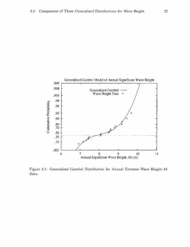
This example concerns the significant wave height HS i n a Southern North Sea location, for which 19 years of hindcast data are available (Danish Hydraulic Institute, 1989). For each of these 19 years, a single storm event has been identified with maximum significant wave height I I , (i.e. the extreme values). This value ranges from IIs = 6.92m (1972/1973) to 9.66m {19S1/19S2). A sorted list of all 19 values is reported in Table 3.1.

This chapter has two sections. The first section deals with the generalized Gumbel model for the significant wave height data. The second section compares the three different generalized distribution models for the same data set.

Finally, it should be noted that a generalized Gumbel model has previously been fit to this data set (Winterstein and Haver, 1991). The results shown here are an improvement in two senses: (1) fitting permits greater accuracy to be achieved in matching moments; and (2) fitting includes a n inverse cubic transformation, which is particularly important in refiecting the narrower-than-Gumbel tails similar to the data in Table 3.1.

24 Chapter 3. Extreme Values: A Generalized Gumbel Example

I Line number i: Data H,, [m]: 9.66 9.44 9.18 9.17 8.85 8.79 8.60 8.58 8.54 8.49 8.09 8.08 8.06 7.47 7.42 7.41 7.31 7.16 6.92

Table 3.1: Listing of annual significant wave height [m] from gumbel .dat. File contains column 2 da ta only; line numbers are inserted here for clarity.

3.1 Generalized Gumbel Results

The annual significant wave height data consists of 19 values listed in Table 3.1. The da ta are stored in the file gumbel.dat. For the sake of clarity they are input in decreasing order; however, this is not required by the program.

The control data are stored in gumbel.in. Table 3.2 lists this file. The first line of this file contains three values. The first value is xmin=0.0, which sets the lower threshold value. Note, however, that this is not used in this case of Gumbel distribution since there is no cutoff value. This threshold value is used when generalized Weibull distribution is fit to the data (see Chapter 2). The second argument, i f l ag= l , indicates that x values are to follow in the file and the program will calculate corresponding cdf values. The third argument, itype=2, indicates that a generalized Gumbel distribution is to be fit to the data in file gumbel. dat. The remaining lines list the actual x values requested.

Output. Table 3.3 lists the corresponding output file gumbel .out for this example. I t also reports the first four moments from these data , as estimated by calmom,

3.2. Comparison of Three Generalized Distributions for Wave Height 25

0.00 1 2 ; XMIN=LOWER THRESHOLD, IFLAG=] T O G E T C D F FOR GIVEN X; I T Y P E = 2 T O F I T GENERALIZED GUMBEL

10.00 9.66 9.44 9.18 9.17 8.85 8.79 8.60 8.58 8.54 8.49 8.09 8.08 8.06

Table 3.2: Listing of input file, gumbel. in, with control data for driver program.

which are used as input to fitting. Finally, the model predicts the first 10 absolute moments, E [ X " ] . Note that these are consistent with the first four moments found for the data. For example, E [ X ' ] = 8.275, the mean value pz, while E [ X Z ] = u$ + p i , or .819' + 8.275'=69.1. Similarly, the predicted third and fourth moments can be shown consistent with those estimated from the data.

As discussed in Chapter 2, note that to use the input files gumbel . in and gumbel . dat with the driver program they must be copied to the files driver. in and driver. dat respectively. The output, written to driver .out, should then be comparable to gumbel . out.

In order to generate a smooth plot of the generalized Gumbel distribution, an input file similar to driver. in with a greater number of input values to compute corresponding CDF values was used. This distribution is plotted in Figure 3.1 along with the observed data values. It appears to capture fairly well the systematic curvature of the data on the Gumbel probability scale used.

3.2 Comparison of Three Generalized Distribu- tions for Wave Height

Because we deal here with annual extreme values, the Gumbel distribution is the natural choice of parent distribution. \Ire may ask, however, what effect is achieved if


Number of Data Processed: 19


Mean : 8.275 Standard Deviation: 0.819

Skewness : -0.053 Kurtosis: 1.905


X : CDF :

10.000 9.660 9.440 9.180 9.170 8.850 8.790 8.600 8.580 8.540 8.490 8.090 8.080 8.060

0.998 0.978 0.937 0.846 0.842 0.690 0.662 0.580 0.572 0.557 0.539 0.427 0.424 0.419

** PREDICTED MOMENTS (FITTING) ** N: E[X**N] :

1.000 0.827E+Ol 2.000 0.691E+02 3.000 0.583E+03 4.000 0.496E+04 5.000 0.426E+05 6.000 0.369E+06 7.000 0.322E+07 8.000 0.282E+08 9.000 0.250E+09 10.000 0.222E+10

Table 3.3: Listing of output file, gumbel .out, produced by driver program.

3.2. Comparison of Three Generalized Distributions for Wave Height

Generalized Gumbel Model of Annual Significant Wave Height

Generalized Gumbel - Wave Height Data 0

.998 -

.995 - h .99 E .98 -

- c) .-

.n E .95 - ? .90 -

6 7 8 9 10 11 Annual Significant Wave Height, Hs [m]

27

Figure 3.1: General ized G u m b e l Distr ibut ion for A n n u a l E x t r e m e W a v e Height-19 D a t a .


Generalized Gumbel Model of Annual Significant Wave Height .999 .998 Generalized Gumbel -

Generalized Gaussian ------ .995 Generalized Weibull ........

3 .99 Wave Height Data 0

2 .98

.95 P .90 - .80 E' .70

S O .30 .10

.oo 1

1-

.o

3

........................................... ............................................................................................

6 7 8 9 10 1 1 Annual Significant Wave Height, Hs [m]

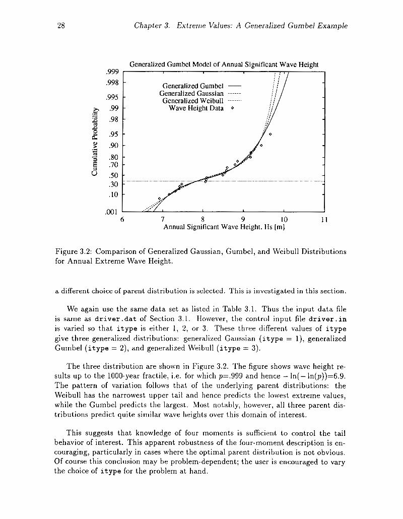
Figure 3.2: Comparison of Generalized Gaussian, Gumbel, and Weibull Distributions for Annual Extreme Wave Height.

a different choice of parent distribution is selected. This is investigated in this section.

We again use the same data set as listed in Table 3.1. Thus the input da ta file is same as d r i v e r . d a t of Section 3.1. However, the control input file d r i v e r . i n is varied so that i t y p e is either 1, 2, or 3. These three different values of i t y p e give three generalized distributions: generalized Gaussian ( i t y p e = l ) , generalized Gumbel ( i t y p e = 2), and generalized Weibull ( i t y p e = 3).

The three distribution are shown in Figure 3.2. The figure shows wave height results up to the 1000-year fractile, i.e. for which p=.999 and hence - In(- ln(p))=6.9. The pattern of variation follows that of the underlying parent distributions: the Weibull has the narrowest upper tail and hence predicts the lowest extreme values, while the Gumbel predicts the largest. Most notably, however, all three parent distributions predict quite similar wave heights over this domain of interest.

This suggests that knowledge of four moments is sufficient to control the tail behavior of interest. This apparent robustness of the four-moment description is en- couraging, particularly in cases where the optimal parent distribution is not obvious. Of course this conclusion may be problem-dependent; the user is encouraged to vary the choice of i t y p e for the problem a t hand.

Chapter 4

Technical Background and Additional Details

4.1 Mot ivat ion

The fitting routine has been developed to modify standard, commonly used distributions to better match observed tail behavior. In particular, cubic distortions of these standard “parent” distributions are sought to match the first four moments of the data. We may then ask why precisely four moments are used to fit the probability distribution of X-and not two, three, five, ten, etc. Conventional models are of lower order, requiring only one or two moments. The problem is that a number of plausible models, with very different tail behavior and hence fatigue reliability, can be fit to the same first two moments. This scatter in reliability estimates is said to be produced by model uncertainty. This is prevalent in low-order, one- or two-moment models. (Note that many common fatigue load models include only one parameter; e.g., the Rayleigh and exponential models.)

To avoid this model uncertainty, which is difficult to quantify, one is led to try to preserve higher moments as well. This will help to discriminate between various models, and hence reduce model uncertainty. The benefit does not come without cost, however: higher moments are more sensitive to rare extreme outcomes, and hence are more difficult to estimate from a limited data set. This is known as statistical uncertainty, which reflects the limitations of our data set.

Thus, our search for an “optimal” model reflects an attempt a t balance between model and statistical uncertainties. Practical experience (e.g., Winterstein, 1988) suggests that four moments are often sufficient to define upper distribution tails over the range of interest. This experience motivates the generalized models developed here. It is again supported by the results of Section 3.2, in which extreme wave heights are insensitive to the choice of parent distribution, once four moments have been specified.

30 Chapter 4. Technical Background and Additional Details

4.2 Underlying Methodology : fitting

The fitting routine begins with a theoretical, 2-parameter “parent” distribution. In the current implementation, the user may choose Gaussian, Gumbel, or Weibull parent distributions. Denoting this parent variable as U , fitting then models the physical random variable X through a cubic transformation of Cl:

X = Q + C l U + c2u2 + c3U3 (4.1) The optimizer adjusts the coefficients c, through an iterative scheme until the difference between the requested skewness, ~ 3 , and kurtosis, a4, (see xmom(3) and xmom(4), section 1.2) and those of the generalized model in Eq. 4.1 ( Q ~ X and a4x) are minimized.

The optimizer also restricts the coefficients so that Eq. 4.1 remains monotonically increasing, producing a well-behaved model that only mildly modifies the underlying parent distribution. This leads, for example, to requiring cg 2 0 so that X in Eq. 4.1 continues to grow as U becomes large. This in turn makes it difficult to model cases with tails that are narrower than those of the parent distribution. In particular, it is difficult to use Eq. 4.1, with positive cg, to model situations in which the desired kurtosis, ~ 4 , is less than that of the parent variable, Q ~ U . In this case fitting inverts the model, seeking to fit a model analogous to Eq. 4.1 in which the roles of X and U are interchanged. (In this view, one seeks to expand the distribution tail of the actual variable X to produce a parent variable U , so that c3 becomes positive.)

Note that this switching between two dual models, based on the size of cy4, occurs automatically within fitting and should be of no consequence to the user. Adding such a dual model, however, has has been found to greatly increase modelling flexi- bility for small kurtosis cases. These have been found to arise both in extreme and fatigue loading applications.

Finally, in whichever form the model is defined, the coefficients c, are chosen to minimize the error e, defined as

e = J ( a 3 - Q3xy + ( a 4 - a4x)2 (4.2) The speed of executing fitting is governed largely by the speed of this optimization; i.e., by the amount of effort (trial c, values) needed to achieve an acceptably small tolerance, eto( . The driver program sets eto,=.Ol for the examples shown. The user can vary this tolerance, with the resulting change in computation time to be expected.

4.3 Underlying Methodology: calmom

To motivate the need for this routine, we must consider a brief background in statistical moment estimation. If we seek to estimate the ordinary mean value E [ X ) = p

4.3. Underlying Methodology: calmom 31

from data XI... X,,, a natural estimate is the simple average value x=Cr=l X’,/n. Similarly, the k-th order “ordinary” moment, E [ X k ] , is naturally estimated by the corresponding average Cy=, Xk/n.

The difficulties arise when we instead seek, as in many applications, to estimate not ordinary but central moments; i.e., of the form pk=E[(X - P ) ~ ] for k=2, 3, 4.... (Note that f i t t i n g input stops a t k=4: or=p2 1 1 2 , a3=p3/p:.’ , and a4=p4 /p i . )

The problem here lies in i t s circular aspect: we must first estimate the unknown first moment p before seeking to estimate p k = E [ ( X - p ) ‘ ] . And, if we use the same data set for both purposes, we typically find too-low estimates of p2, p3, p 4 , etc. because our p value is artificially tuned to best match the mean of the observations. Those exposed to a standard statistics coursc will best recognize this phenomenon when estimating the variancc p 2 : to inflate the sample variance to account for this bias, the sum of squared deviations is divided by n - 1 rather than n.

While unbiased estimates of the higher moments 113, p4, ... are less familiar, they are available in the statistical literature (Fisher, 19%):

p3 = m3 (4.5) ( n - l ) ( n - 2)

in terms of the sample central moment mk=C:,l(X; - X)‘/n. Eq. 4.4 is the conventional result for the sample variance.

Remaining Bias. Finally, the routine calmom uses these results to estimate the quantities oz by p:.5, a3 by p 3 / ( p ; . 5 ) , and a4 by /id/(&). Because these vary nonlinearly with p,,, they may still contain some bias although the p,, estimates do not.

For example, if we fit a Gumbel model to the 19 wave height data from Chapter 3, the true skewness and kurtosis values are 1.14 and 5.40. However, simulating 10000 data sets of size n=19 and running each through calmom, we find on average the skewness 0.79 and kurtosis 3.S9 (Winterstcin and Haver, 1991).

To address this problem, the f i t t i n g routine has a n automatic check for remaining bias through simulation. This is why n d a t a is given as an input parameter. After f i t t i n g constructs a distribution with moments from the input array xmom, many similar data sets (of size n d a t a ) are simulated from this distribution. If the moments

32 Chapter 4. Technical I3ackground and Additional Details

.999

.998

.995 .99 .98

.95

.90

.80

.70 S O .30 .10

.001

Generalized Gumbel Model of Annual Significant Wave Height

- Generalized Gumbel (unbiased) -

- Generalized Gumbel (uncorrected) ------ Wave Height Data 0 -

- -

- -

6 7 8 9 10 11 Annual Significant Wave Height, Hs [m]

Figure 4.1: Effect of Ignoring Bias: Wave Height Example.

predicted from calmom differ appreciably on average from the input values, new theoretical estimates of the moments are constructed. This estimation-simulation loop is continued iteratively until satisfactory convergence is found.

Note that the fitting routine does not perform this simulation if its input parameter ndata > 100. This value can be hard-wired if the user wishes to bypass this option. Figure 4.1 shows the effect of enabling this “unbiased” option (the default) and disabling it (using “raw” moments from calmom directly) for the generalized Gumbel model produced for the example given in Chapter 3. There is relatively little difference found in these cases. Larger effects may be found for cases of (1) fewer data and/or (2) distributions with broader tails.

4.4 Notes on Usage

The fitting routine has limiting conditions that users should note. When these conditions are encountered, appropriate error messages are written to the output file/device corresponding to the input logical unit number ioout. This section explains the meaning of these messages and discusses other details regarding fitting usage.

4.4. Notes on Usage 33

4.4.1 Errors in Matching Moments

Note that in most practical cases, the coefficients c, in Eq. 4.1 can be chosen so that the error e , as given in Eq. 4.2, falls within the user-defined tolerance limit ctol . In rare cases the minimized error exceeds c to l . In these cases fitting writes an error message indicating the magnitude of c, the error norm of the skewness and kurtosis in Eq. 4.2.

4.4.2 Lower Tail Limiting Values

Lower tail limiting values are only a problem when the parent distribution is Weibull. In this case the variable I/ in Eq. 4.1 has Weibull distribution, and hence a minimum value of 0. Because Eq. 4.1 is monotonic, the corresponding smallest possible value of the physical variable X is G. This physical lower limit G, can be either greater or less than zero, since the optimized Weibull model in Eq. 4.1 will not in general have its 5 intercept a t exactly zero.

This may lead to situations that seem anomalous. If the lower limit G, is negative, for example, fitting may estimate negative values of X for probabilities near zero. Conversely, if the lowest possible value G, is positive, a n input X value below G, cannot occur and fitting will return a zero cumulative probability (CDF=O). When xmin is not zero the situation is entirely analogous: Q may be greater or less than xmin.

In practice we believe this to be a minor issue for the following reasons:

0 The routine fitting is intended for applications where large X values (upper distribution tails) are crucial. This is the motivation for preserving higher moments. Its accuracy at the lower end of the distribution may not be of great concern.

0 If we wish to preserve a positive range of values, one can easily introduce a transformation to the data. For example, apply fitting not to the physical variable X but rather Y=ln(X), based on the first four moments of Y . Then the reverse transformation X=exp(Y) will still be positive.

0 The routine fitting is intended for applications where the true distribution is not too different than a Weibull model would predict. In such cases we may expect the nonlinear terms (proportional to Q, c2, and cg) in Eq. 4.1 to be relatively small on average relative to the linear term. Thus, compared to the range of likely variation of X values, Q may seem to lie rather “close” to zero.

34

References

Ang, A., and W. Tang, 1975, Probability Concepts in Engineering Planning and Design, Volume I Basic Principles, John Wiley and Sons, Inc.

Benjamin, J.R., and C.A. Corncll, 1970, Probability, Statistics, and Decision for Civil Engineers, McGraw-Hill Book Co.

Coleman, C., and B. McNiff, 1989, Final Report: Dynamic Response Testing of the Northwind 100 Wind Turbine, Subcontractor Report, SERI Cooperative Research Agreement No. DE-FC02-86CH10311, Solar Energy Research Institute, Golden, CO, 4OPP.

Danish Hydraulic Institute, 1989, Environmental Design Conditions and Design Procedures for Oflshore Structures, Copenhagen.

Fisher, R.A., 1928, “Moments and Product Moments of Sampling Distributions,” Proceedings of the London Mathematical Society, Vol. 30, pp. 199-238.

Fuchs, H., and R. Stephens, 1980, Metal Fatigue in Engineering, John Wiley and Sons, Inc.

Veers, P.S., C.H. Lange, S.R. Winterstein, and ‘T.A. Wilson, 1994, Users Manual for FAROW: A Computer Analysis of the Fatigue and Reliability of Wind Turbine Components, SAND94-2460, Sandia National Laboratories, Albuquerque, New Mex- ico.

Winterstein, S. R. 1988, “Nonlinear Vibration Models for Extremes and Fatigue,” Journal of Engineering A/lechanics, Vol. 114, No. 10, Oct,ober, 1988.

Winterstein, S. R., and S. Haver, 1991, “Statistical Uncertainties in Wave Heights and Combined Loads on Offshore Structures,” 9th International Symposium on 08- shore Mechanics and Arctic Engineering, Houston, Texas, ASME.

Winterstein, S.R., and C.1-I. Lange, 1994, “Load Rllodcls for Fatigue Reliability from Limited Data,” Wind Energy - 1994, ASME.

35

Appendix A

Driver Source Code Listing

36 Appendix A . Driver Source Code Listing

C C C C C C C C C C C C C C C C

C

C

C

XMIN LOWER THRESHOLD DATA VALUE USED IN THE ANALYSIS IFLAG INPUT/OUTPUT FLAG:

IFLAC = O.....FINDS X FOR INPUT CDF VALUES IFLAC = l.....FINDS CDF FOR INPUT X VALUES

ITYPE CONTROL VARIABLE TO CHOOSE THE GENERALIZED DISTRIBUTION TYPE

ITYPE = 1 :FIT GENERALIZED GAUSSIAN DISTRIBUTION ITYPE = 2 :FIT GENERALIZED GUMBEL DISTRIBUTION ITYPE = 3 :FIT GENERALIZED WEIBULL DISTRIBUTION

X (NXMAX) LEVELS OF X AT WHICH DISTRIBUTION IS REPORTED CDF(NXMAX) CDF VALUES (NON-EXCEEDENCE PROBABILITIES) FOR

NXMAX MAXIMUM NUMBER OF X OR CDF VALUES REQUESTED NX ACTUAL NUMBER OF X OR CDF VALUES REQUESTED

EACH X LEVEL

READ(IOIN,*) XMIN,IFLAG,ITYPE IF (ITYPE .NE. 3) XMIN = O.dO IF (IFLAG. EQ. 0) THEN

DO 10 IX = 1,NXMAX 10 READ(IOIN,*,ERR=30,END=30) CDF(1X)

READ CDF VALUES IF IFLAG=O ELSE

DO 20 IX = 1,NXMAX 20 READ(IOIN,*,ERR=30,END=30) X(1X)

READ X VALUES IF IFLAG=l ENDIF

30 NX = IX - 1

C C C C C

40

DATA(NDMAX) ARRAY OF INPUT DATA FOR WHICH MOMENTS ARE FOUND NDMAX MAXIMUM NUMBER OF INPUT DATA PERMISSIBLE NDATA ACTUAL NUMBER OF INPUT DATA

NDATA=O READ(IODAT,*,ERR=50,END=50) X1 NDATA=NDATA+l

GO TO 40 DATA ( ND ATA) =X 1

37

C C XMOM (4) ARRAY OF FOUR C XMOM(1) = C XMOM(2) = C XMOM(3) = C XMOM(4) = C

MOMENTS COMPUTED FROM DATA: MEAN STANDARD DEVIATION SKEWNESS KURTOSIS

CALL CALMOM(XMOM,DATA,NDATA,NDMAX,XMIN,ITYPE) C c----------------------------------------------------------- C

WRITE OUTPUT

IF (ITYPE .EQ. 3) THEN WRITE(IOOUT,900) ’ Lower Threshold Value:’, XMIN ENDIF WRITE(IOOUT, * ) ’ Number of Data Processed:’, NDATA WRITE(IOOUT, * ) ’ ’ WRITE(IOOUT, * ) ’ ** MOMENT RESULTS **’ WRITE(IOOUT, * ) ’ ’ WRITE(IOOUT,900) ’ Mean: ’ , XMOM(1) WRITE(IOOUT,900) ’ Standard Deviation:’, XMOM(2) WRITE(IOOUT,900) ’ Skewness:’, XMOM(3) WRITE(IOOUT,900) ’ Kurtosis:’, XMOM(4) WRITE(IOOUT, * ) ’ ’

C c--------------------- CALL FITTING TO ESTIMATE X FOR GIVEN CDF (IFLAG=O) C OR CDF FOR GIVEN X (IFLAG=l) C C ETOL ERROR TOLERANCE IN MATCHING OBSERVED MOMENTS C . . . HERE WE ACCEPT 0.01 ERROR---USER CAN ALTER C C PMOM( 10) ARRAY OF PREDICTED ABSOLUTE MOMENTS FROM MODEL C PMOM(1) = PREDICTED AVERAGE OF X**N, N=l..10 C

ETOL = .01DO CALL FITTING(ITYPE,XMOM,NDATA,XMIN,X,CDF,NX,PMOM,IFLAG,IOO~,ETOL)

OUTPUT

38 Appendix A. Driver Source Code Listing

DO 60 IX = 1 , NX 60 WRITE(IOOUT,~OI) X(IX),CDF(IX)

WRITE(IOOUT, * WRITE(IOOUT, * ) ** PREDICTED MOMENTS (FITTING) ** ’ WRITE(IOOUT, * ) ’ ’ WRITE(IOOUT, * N: E[X**N] : ’ WRITE(IOOUT, * )

DO 70 IX = 1 , 10 70 WRITE(IOOUT,902) REAL(IX),PMOM(IX)

C 900 FORMAT(A26, F10.3) 901 FORMAT(16X,2F10.3) 902 FORMAT(16X, F10.3,E10.3)

C STOP END

3 9

DISTRIBUTION:

R. E. Akins Washington & Lcc University P.O. Box 735 Lexington, VA 21450

H. Ashlcy Dcpt. of Acronautics and

Stanford University Stanford, CA 94305

Astronautics Mechanical Engr.

E. Ausman Polarconsort Alaska 1503 W. 33rd Avenue Suite 3 10 Anchoragc, AK 99530

B. Bcll FloWind Corporation 990 A Strcct Suite 300 San Rafacl, CA 91901

K. Bcrgcy University of Oklahoma Aero Engineering Dcpartmcnt Norman, OK 73069

J. R. Birk Electric Powcr Research Institute 3412 Hillview Avcnuc Palo Alto. CA 94304

C. P. Butterfield NREL 16 17 Cole Boulcvard Golden, CO 8040 1

G. Bywaters New World Powcr Tcchnology Ccnter Bos 659 Morctown,VT 05660-0659

R. N. Clark USDA Agricultural Research Service P.O. Drawcr 10 Bushland. TX 790 12

C. Colcman Northern Powcr Systems Box 659 Moretown, VT 05660

E. A. DcMeo Electric Powcr Research Institutc 34 12 Hillvicw Avenue Palo Alto, CA 94301

0. Dyes Wind/Hydro/Occan Div. U.S. Departmcnt of Encrgy 1000 Independcncc Avenue, SW Washington, DC 20585

A. J . Eggers, Jr. RANN, Inc. 260 Shcridan Ave., Suite 413 Palo Alto. CA 91306

D. M. Egglcston DME Engineering P.O. Box 5907 Midland, TX 79701-5907

P. R. Goldman Wind/Hydro/Occan Division U.S. Dcpartnicnt of Encrgy 1000 Indcpendcncc Avcnue Washington. DC 20585

I. J. Graham Dept. of Mechanical Engineering Southern University P.O. Box 9145 Baton Rouge, LA 70813-9145

G. Gregorck Acronautical & Astronautical

Ohio State University 2300 West Case Road Columbus, OH 43220

Dept.

C. Hanscn University of Utah Departmcnt of Mechanical Engineering Salt Lake City, UT 84 1 12

40

R. Heffernan Kcnetech Windpower, Inc. 6952 Preston Avenue Livermore, CA 94550

L. Hclling Librarian National Atomic Museum Albuquerque, NM 87 185

T. Hillesland Pacific Gas and Electric Co. 3400 Crow Canyon Road San Ramon. CA 94583

E. N. Hinrichscn Power Tcchnologics, Inc. P.O. Box 1058 Schenectady, NY 12301-1058

S. Hock Wind Energy Program NREL 1617 Cole Boulevard Golden, CO 80101

W. E. HolIey Kenetech Windpower 6952 Preston Avenue Livermore, CA 91550

M. A. Ilyan Pacific Gas and Elcctric Co. 3400 Crow Canyon Road San Ramon, CA 94583

B. J. Im McGillim Research 4903 Wagonwhccl Way El Sobrante, CA 94803

K. Jackson Dynamic Design 123 C Street Davis, CA 95616

0. Krauss Division of Engineering Research Michigan State University East Lansing, MI 48825

C. Lange Civil Engineering Dept. Stanford University Stanford, CA 91305

G. G. Lcigh New Mcsico Engineering

Research Institute Campus P.O. Box 25 Albuqucrque, NM 87 13 1

A. Liniecki Mechanical Engineering Department San Jose State University One Washington Square San Jose. CA 95 192-0087

R. R. Loose. Dircctor Wind/Hydro/Ocean Division U.S. Department of Energy 1000 Indcpendencc Ave., SW Washington, DC 20585

R. Lynctte AWT/RLA 425 Pontius Avcnue North Suitc 150 Scattle, WA 98 109

D. Malcolm A WTIRLA 425 Pontius Avcnue North Suite 150 Scattle. WA 98109

J. F. Mandell Montana State University 302 Cableigh Hall Bozeman, MT 597 17

R. N. Mcroney Dept. of Civil Engineering Colorado Statc University Fort Collins, CO 80521

P. Migliore NREL 16 17 Cole Boulevard Goldcn, CO 8010 1

A. Mikhail Zond Systems, Inc. 13000 Jameson Road P.O. Box 1910 Tchachapi, CA 93561

S. Miller 162636 NE 19th Place Bcllcvue. WA 98008-2552

41

R. H. Monroe Gougeon Brothers 100 Patterson Avenue Bay City, MI 48706

D. Morrison New Mexico Engineering

Research Institute Campus P.O. Box 25 Albuquerque, NM 87 13 1

W. Musial NREL 1617 Cole Boulevard Golden, CO 8040 1

NWTC Library NREL 16 17 Cole Boulevard Golden, CO 8040 1

V. Nelson Department of Physics West Texas State University P.O. Box 248 Canyon, TX 79016

G. Nix NREL 16 17 Cole Boulevard Golden. CO 8040 1

J. W. Oler Mechanical Engineering Dcpt. Texas Tech University P.O. Box 4289 Lubbock, TX 79409

R. Osgood NREL 1617 Cole Boulevard Golden, CO 8040 1

M. Papadakis Aero Engineering Department Wichita State University Wichita, KS 67260-0014

C. Paquette The American Wind Energy Association 122 C Street NW Fourth Floor Washington, DC 20002

R. G. Rajagopalan Aerospace Engineering Department Iowa State University 404 Town Engineering Bldg. Amcs. IA 5001 1

R. L. Scheffler Southern California Edison Research and Development Dept Room 497 P.O. Box 800 Rosemead, CA 9 1770

L. Schienbein Battclle-Pacific Northwest Laboratory P.O. Box 999 Richland, WA 99352

T. Schweizcr Princeton Economic Research, lnc. 1700 Rockville Pike Suite 550 Rockville, MD 20852

J. Sladky, Jr. Kinetics Group, Inc. P.O. Box 1071 Mercer Island, WA 98010

M. Snyder Aero Engineering Department Wichita State University Wichita, KS 67208

L. H. Soderholm Agricultural Engineering Room 2 13 Iowa State University Ames, IA 50010

K. Starcher AEI West Texas State University P.O. Box 248 Canyon, TX 79016

W. J. Stecley Pacific Gas and Electric Co 3400 Crow Canyon Road San Ramon, CA 94583

F. S. Stoddard Dynamic Design-Atlantic Office P.O. Bos 1373 Amherst, MA 0 1004

42

W. V. Thompson 4 10 Ericwood Court Manteca, CA 95336

R. W. Thresher NREL 1617 Colc Boulevard Golden, CO 80401

K. J. Touryan NREL 16 17 Colc Boulevard Golden. CO 8040 1

W. A. Vachon W. A. Vachon & Associates P.O. Box 149 Manchester, MA 0 1941

B. Vick USDA, Agricultural Research Service P.O. Drawer 10 Bushland, TX 790 12

V. Wallace FloWind Corporation 990 A Street, Suite 300 San Rafael, CA 9490 1

L. Wendell Battelle-Pacific Northwest

Laboratory P.O. Box 999 Richland, WA 99352

W. Wcntz Aero Engineering Department Wichita Statc University Wichita, KS 67208

R. E. Wilson Mechanical Engineering Dept. Oregon State University Corvallis, OR 9733 1

S. R. Wintcrstein Civil Engineering Departrncnt Stanford University Stanford, CA 94305

B. Wolff Rcncwablc Energy Program Manager Conservation and Renewable Encrgy System 69 18 NE Fourth Plain Boulevard Suitc B Vancouver. WA 9866 1

M. Zuteck MDZ Consulting 93 1 Grove Strcct Kemah, TX 77565

S. Schuck Renewable Technology Pacific Powcr P.O. Box 5257 GPO Sydney, New South Walcs 200 1 AUSTRALIA

V. Lacey Indal Technologies, Inc. 3570 Hawkestone Road Mississauga, Ontario L5C 2V8 CANADA

A. Lancville Faculty of Applied Science University of Sherbrooke Sherbrookc, Qucbcc J 1 K 2R1 CANADA

B. Masse Institut de Recherche d'Hydro-Quebec 1800, Montcc Stc-Julic Varennes, Quebec J3X 1 S 1 CANADA

1. Paraschivoiu Dcpt. of Mechanical Engineering Ecole Polytechnique CP 6079 Succursalc A Montreal, Quebec H3C 3A7 CANADA

R. Rangi Manager, Wind Tcchnology Dcpt. of Energy, Mincs and Resources 580 Booth 7th Floor Ottawa, Ontario K 1 A OE1 CANADA

4 3

P. Vittecoq Faculty of Applied Sciencc University of Sherbrooke Sherbrooke, Quebec J lK 2R1 CANADA

T. Watson Canadian Standards Association 178 Resdale Boulevard Rcxdale, Ontario M9W 1R3 CANADA

P. H. Madsen Riso National Laboratory Postbox 49 DK-4000 Roskilde DENMARK

T. F. Pedersen Riso National Laboratory Postbox 49 DK-4000 Roskildc DENMARK

M. Pederscn Technical University of Denmark Fluid Mechanics Dept. Building 404 Lundtoftevej 100 DK 2800 Lyngby DENMARK

H. Petersen Rim National Laboratory Postbos 49 DK-4000 Roskilde DENMARK

A. F. Abdel Azim El-Sayed Dept. of Mechanical Design &

Zagazig University 3 El-lais Strcct Zeitun Cairo 11321 EGYPT

Powcr Engineering

M. Anderson Renewable Energy Systems, Ltd. Eaton Court, Maylands Avenuc Hemel Hempstead Herts HP2 7DR ENGLAND

M. P. Ansell School of Material Science University of Bath Claverton Down Bath BA27AY Avon ENGLAND

A. D. Garrad Garrad Hasson 9-1 1 Saint Stephen Street Bristol BSl 1EE ENGLAND

D. I. Page Energy Technology Support Unit B 156.7 Hanvell Laboratory Osfordshire, OX 1 1 ORA ENGLAND

D. Sharpe Dcpt. of Aeronautical Engineering Quccn Mary College Mile End Road London, El 4NS ENGLAND

D. Taylor Alternative Energy Group Walton Hall Open University Milton Keynes MK7 6AA ENGLAND

P. W. Bach Netherlands Energy Research Foundation, ECN P.O. Bos 1 NL-1755 ZG Petten THE NETHERLANDS

J. Beurskens Programme Manager for

Renewable Energies Netherlands Energy Research

Foundation ECN Westerduinweg 3 P.O. Bos 1 1755 ZG Petten (NH) THE NETHERLANDS

0. de Vries National Aerospace Laboratory Anthony Fokkenveg 2 Amsterdam 10 17 THE NETHERLANDS

4 4

J. B. Dragt Institute for Wind Energy Faculty of Civil Engineering Dclft University of Tcchnology Stevinwcg 1 2628 CN Delft THE NETHERLANDS

R. A. Galbraith Dcpt. of Aerospace Engineering James Watt Building University of Glasgow Glasgow G 12 8QG SCOTLAND

M. G. Rcal, President Alpha Real Ag Feldeggstrasse 89 CH 8008 Zurich SWITZERLAND

M.S. 0167 M.S. 0437 M.S. 0439 M.S. 0439 M.S. 0439 M.S. 0443 M.S. 0443 M.S. 0557 M.S. 0557 M.S. 0557 M.S. 0557 M.S. 0557 M.S. 0615 M.S. 0615 M.S. 0708 M.S. 0708 M.S. 0708 M.S. 0708 M.S. 0708 M.S. 0708 M.S. 0708 M.S. 0708 M.S. 0708 M.S. 0833 M.S. 0836 M.S. 0836 M.S. 0100

M.S. 0619 M.S. 0899 M.S. 9018

J. C. Clausen, 12630 E. D. Recdy, 1562 C. R. Dohrmann, 1434 D. W. Lobitz, 1434 D. R. Martinez, 1434 1. G. Arguello, 1561 H. S. Morgan, 156 1 T. J. Baca, 2741 T. G. Carne, 2741 B. Hansche, 2741 G. H. James Il l , 2741 J. P. Lauffer, 2741 A. Beattie, 2752 W. Shurtleff, 2752 H. M. Dodd, 6214 (50) T. D. Ashwill, 6214 D. E. Berg, 6214 D. P. Bunvinklc, 6214 M. A. Rumsey, 6214 L. L. Schlutcr, 6214 H. J. Sutherland, 62 14 P. S. Vcers, 6214 T. A. Wilson, 6214 J. H. Strickland, 1552 G. F. Homicz, 15 16 W. Wolfc, 1516 Document Processing, 761 3-2 (2)

For DOE/OSTI Technical Publications, 126 13 Technical Library, 13414 (5) Central Technical Files, 8523-2

A Subroutine to Fit Four-Moment Probability … · The user may select here between Gaussian,...

Documents

Transcript of A Subroutine to Fit Four-Moment Probability … · The user may select here between Gaussian,...