Auton Robot (2015) 39:1–23DOI 10.1007/s10514-015-9424-5

A suboptimal and analytical solution to mobile robot trajectorygeneration amidst moving obstacles

Jun Peng · Wenhao Luo · Weirong Liu ·Wentao Yu · Jing Wang

Received: 11 May 2013 / Accepted: 3 January 2015 / Published online: 4 February 2015© Springer Science+Business Media New York 2015

Abstract In this paper, we present a suboptimal and ana-lytical solution to the trajectory generation of mobile robotsoperating in a dynamic environment with moving obstacles.The proposed solution explicitly addresses both the robotkinodynamic constraints and the geometric constraints dueto obstacles while ensuring the suboptimal performance toa combined performance metric. In particular, the proposeddesign is based on a family of parameterized trajectories,which provides a unified way to embed the kinodynamic con-straints, geometric constraints, and performance index intoa set of parameterized constraint equations. To that end, thesuboptimal solution to the constrained optimization problemcan be analytically obtained. The solvability conditions to theconstraint equations are explicitly established, and the pro-posed solution enhances the methodologies of real-time path

Jun Peng (first author) and Wenhao Luo (second author) contributedequally to this work.

J. Peng · W. Liu (B) · W. YuSchool of Information Science and Engineering, Central SouthUniversity and Hunan Engineering Laboratory for AdvancedControl and Intelligent Automation, Changsha 410083, Chinae-mail: weirong_liu@126.com; frat@csu.edu.cn

J. Penge-mail: pengj@csu.edu.cn

W. Yue-mail: wentaoyu@gmail.com

W. LuoRobotics Institute, School of Computer Science,Carnegie Mellon University, Pittsburgh, PA 15213, USAe-mail: luo@cmu.edu; whluo12@gmail.com

J. WangDepartment of Electrical and Computer Engineering,Bradley University, Peoria, IL 61525, USAe-mail: jingwang@bradley.edu

planning for mobile robots with kinodynamic constraints.Both the simulation and experiment results verify the effec-tiveness of the proposed method.

Keywords Nonholonomic mobile robots · Trajectorygeneration · Moving obstacles · Kinodynamic constraints ·Optimization

1 Introduction

During the past decades, trajectory generation for mobilerobots moving in a dynamic environment has received con-siderable attention. Two major concerns towards that topicare problems of feasibility and optimality (LaValle 2006).The feasibility is mainly concerned with the kinematic con-straints of robots such as nonholonomic constraints , or kino-dynamic constraints such as velocity and acceleration bounds(Li and Canny 1992). It is desirous for the robot to generate afeasible trajectory on-line that also satisfies certain optimal-ity requirements.

To consider robot kinematic constraints, some canonicalmethods as Kim and Khosla (1992), Borenstein and Koren(1991) that directly focus on geometric space have beenrevised by alternative techniques. One approach is to mainlystudy on the path planner towards nonholonomic constraintsand try to obtain the steering method to drive a robot to apre-determined configuration. Without obstacles, discretiz-ing control method is proposed in Barraquand and Latombe(1991), Divelbiss and Wen (1997) to integrate the motionequations to obtain a feasible path. A reverse motion basedcase has been adapted to obstacle-cluttered environment tooptimize the path length (Bicchi et al. 1995). In Duleba andSasiadek (2003) Newton algorithm and Jacobian matrix areused to solve energy optimization without obstacles. More-

123

2 Auton Robot (2015) 39:1–23

over, the planning problem can be directly considered as anoptimal control problem using Hamiltonian equations andPontriagin’s maximum principle in Reister and Pin (1994),Balkcom and Mason (2002). Input parameterizations areused in Murray and Sastry (1993), Tilbury and Murray (1995)to design steering input and represent the trajectories bysinusoidal, polynomial, or piecewise constant functions tosmooth control inputs. Alternative methods (Dong and Guo2005; Fliess et al. 1995) generate smooth trajectories basedon differential flatness approach. However, moving obstaclesare seldom considered in those works, and optimality couldbe hard to formulate with kinematic constraints (LaValle2006). Recent work in Bhattacharya et al. (2012) proposesa graph-search based method to plan homologous trajecto-ries with topological constraints in Euclidean configurationspaces.

Approaches that directly plan nonholonomic trajectoriesbecomes a new topic. This kind of solutions concentrateson trajectory generation and corresponding steering controlbased on the property of nonholonomic systems. Probabilis-tic roadmap methods (PRM) (Kindel et al. 2000; Ladd andKavraki 2004; van den Berg and Overmars 2007) and rapidly-exploring random trees (RRTs) methods (Cheng et al. 2008;ucan and Kavraki 2012; Karaman and Frazzoli 2010; LaValleand Kuffner 1999) are introduced to search for feasible pathsand incorporate both vehicle’s kinematic and dynamic con-straints. In these works obstacle-free space is divided in termsof random samples and connection of these samples form thecorresponding feasible trajectory. Grid-based discretizationmethod is also used in ucan and Kavraki (2012) to estimatethe coverage of the state space and could help to detect less-explored areas with complex dynamics. Most of such algo-rithms mainly discuss about the robot moving in static envi-ronment, and plenty of moving obstacles could make it hardfor random trees to converge to a certain optimal path.

Recently, another kind of search-based method using “lat-tice graphs” has been proven to be efficient and attractiveworking in complex dynamic environments. The concept isfirst developed in Pivtoraiko et al. (2009), wherein the idea isto divide the configuration space into a set of cells (reachablestates) and construct a state lattice at first for graph searchesusing heuristic search algorithms such as A* and D* Lite(Koenig and Likhachev 2002), and subsequently search for aspecific combination of actions/edges (control/motion prim-itives) sequences in the action space to drive the robot alongthe feasible path. In order to address real-time planning forhigh-speed robot moving over large distances in dynamicenvironment, Likhachev and Ferguson (2009) introduced anovel multi-resolution lattice state/action space and employthe incremental search algorithms such as Anytime DynamicA* (AD*) to more efficiently find global and feasible subopti-mal solutions among obstacles. However, the resulting purelyspatial trajectories by Likhachev and Ferguson (2009) may

fail to deal well when operating in cluttered environmentsfull of dynamic obstacles, since it does not consider timeas a state variable. Considering such a problem, Kushleyevand Likhachev (2009) proposes a novel data structure, “atime-bounded lattice”, to merge both short-term planningwith concerns of time and long-term planning without time.Leveraging the time horizon from the time-bounded latticeidea (Kushleyev and Likhachev 2009; Narayanan 2012) pro-poses an anytime planners to find an initial solution quicklyand then continue to optimize it as time allows. In thosemethods, however, as pointed out in Likhachev and Fergu-son (2009), Howard (2007) no explicit representation of cur-vature and the rigidness of the discretized motion-primitivesmay result in discontinuous motions at the junctions betweenmotion primitives and locally less optimal performance forthe rendered paths.

Compared to the search-based methods, the real-timeapproaches of analytical motion planning are in a way morecomputational simple and efficient for working in localdynamic environment. A new parametric solution has beenproposed in Qu et al. (2004) to analytically consider bothkinematic constraints and moving obstacles with the utiliza-tion of the chained form/differential flatness (Lvine 2009;Luca et al. 1998), and the velocity obstacles method in Fior-ini and Shiller (1993), Shiller et al. (2001). The concept of‘Velocity Obstacle’ is extended in Wu and How (2012) toincorporate moving obstacles that have constrained dynamicsbut move unpredictably. Based on Qu et al. (2004), extendedworks in Yang et al. (2005, 2010) have introduced energy-optimal and path length-optimal methods. For those meth-ods, however, lack of considering robot kinodynamic con-straints and special need for intermediate configuration toovercome the vertical singularity could weaken both feasi-bility and optimal effectiveness of the generated paths. In Guoand Tang (2008), Yuan and Shim (2011), Guo et al. (2007),Hashim and Tien-Fu (2009) different trajectory models areused to avoid curvature discontinuities and vertical singular-ities, while the optimization is not completely solved in Guoand Tang (2008). Parameters of the robot dynamic model inYuan and Shim (2011) is often difficult to obtain. Liu andSun (2011) provides a special cost function to present opti-mal options whereas it can only deal with statistic obstacleswith prior knowledge of environment. Further research onhigher dimensional states such as velocity and acceleration(kinodynamic) and complete optimization are needed to bet-ter extend application of analytical solutions.

In this paper, we propose a suboptimal and analyticalsolution for mobile robot on-line trajectory generation inthe presence of moving obstacles. First, we parameterizethe family of trajectories by two time-variant polynomialsand based on the flatness differential property as well as anexplicit consideration of robot kinematic constraint, high-dimensional robot boundary states are substituted to make

123

Auton Robot (2015) 39:1–23 3

trajectories controlled by two freely adjustable parameters.As a result, importantly, the kinodynamic constraints can behandled together with geometric constraints due to obstacles,and the trajectory generation problem can then be recast asoptimizing the two free parameters based on a set of con-straint equations. By defining two optimal indices to quantifythe minimum control energy consumption and the shortestpath length, respectively, the suboptimal solution in terms ofthe two parameters can be obtained in closed form, allowinghighly efficient on-line computation. Particularly, the opti-mization process is simplified and analytically solved in theproposed 2D parameter space, leading to improved subopti-mal solutions that render good suboptimal and feasible tra-jectories in real-time.

This paper further extends the work in Qu et al. (2004),Guo and Tang (2008), and Guo et al. (2007). Compared withthose existing results, the main contributions of this paperare as follows. (1) Higher-dimensional states such as veloc-ity and acceleration are considered for the robot, allowing toexplicitly address the kinodynamic constraints, and to avoidsingularity problem as well as discontinuous or incompatiblecontrol at boundary states. (2) Optimization problem is flex-ibly and analytically addressed on a 2D parameter space byconsidering an adjustable combined metric consisting of bothenergy optimality and length optimality, making the obtained2D analytical suboptimal solutions in principle outweigh the1D solutions in the existing works and still run in real-time.(3) Solvable conditions are established with the discussionof remedies for the possible unsolvable constraint equations.

This paper is organized as follows. Section 2 formulatesthe trajectory generation problem. In Sect. 3, two optimalperformance indices of the trajectories are introduced andintegrated with a combined solution form without address-ing constraints. In Sect. 4, kinodynamic constraints and thecollision avoidance are taken into account. Framework ofthe suboptimal solutions on the parameter space are clearlyillustrated. Simulation and experiment results are included inSect. 5 to illustrate the effectiveness of the proposed method.Section 6 concludes the paper.

2 Problem formulation

Consider the trajectory generation problem for a car-likemobile robot. The mobile robot is represented by a circum-circle and conforms to nonholonomic constraints. The frontwheels of the mobile robot are steering wheels and the rearwheels are driving wheels with a fixed forward orientation,and the mathematical model of the robot is described by⎡⎢⎢⎣xyθ

ϕ

⎤⎥⎥⎦ =

⎡⎢⎢⎣

cos θ

sin θ

tan ϕ/ l0

⎤⎥⎥⎦ u1 +

⎡⎢⎢⎣

0001

⎤⎥⎥⎦ u2 (1)

Fig. 1 The mobile robot moving in the dynamic environment

where (x, y) represents the Cartesian coordinates of the mid-dle point of the rear wheel axle, θ is the orientation of therobot body with respect to the X -axis, ϕ is the steering angle, lis the distance between the front and rear wheel-axle centers,u1 the linear velocity of the driving wheels and u2 the steeringvelocity of the guiding wheels. Note that ϕ ∈ (−π

/2, π/2)

due to the structure constraint of the robot.Assume that the robot moves in a working region as shown

in Fig. 1, where moving obstacles are represented by simplecircumcircles.

In this paper, the objective is to design a trajectory genera-tion method to steer the robot moving from the starting pointO0(x0, y0) at the initial time t0 to the final point O f (x f , y f )

at the final time t f = t0 + T while satisfying kinodynamicconstraints and certain optimality requirements, where T isa given constant.

3 An optimal and analytical solution framework

3.1 Trajectory paramterization

The proposed trajectory generation solution is based on thetypical trajectory parameterization method, as studied in Quet al. (2004), Guo et al. (2007). Specifically, we parameterizethe family of trajectories of the robot as two polynomials interms of time t

x (t) = [c0 c1 c2 . . . cp

]f (t)

y (t) = [d0 d1 d2 . . . dp

]f (t) (2)

with f (t) = [1 t t2 t3 . . . t p

]T, integer p > 0 and

ci , di , i = 0, . . . , p are some constants be determined toaddress the system model constraints, collision avoidanceand optimal performance in a unifying way.

The polynomial order p plays an important role in solvingthe posed optimal trajectory generation problem. In essence,

123

4 Auton Robot (2015) 39:1–23

p = 5 suffices to determine a unique solution for the para-meterized trajectory defined in (2) based on the availabletrajectory boundary conditions at t0 and t f . In this paper pis specified by 6, which then releases two more free parame-ters c6 and d6 so as to deal with additional constraints fromcollision avoidance and optimization.

Assume that the initial driving velocity v0�= u1(t0), the

initial acceleration a0�= u1(t0), the final driving veloc-

ity v f�= u1(t f ), and the final acceleration a f

�= u1(t f )are known. Thus, together with the initial and final stateboundary conditions q0 = [x0, y0, θ0, ϕ0]T and q f =[x f , y f , θ f , ϕ f

]T , we can construct a higher-dimensionalboundary conditions such as q∗

0 = [x0, y0, θ0, ϕ0, v0, a0]Tand q∗

f = [x f , y f , θ f , ϕ f , v f , a f

]T . Considering the kine-matic model of the mobile robot, then we have

dxdt

∣∣t0 = v0 cos θ0,dydt

∣∣t0 = v0 sin θ0

d2xdt2

∣∣t0 = a0 cos θ0 − v20 tan ϕ0

l sin θ0

d2 ydt2

∣∣t0 = a0 sin θ0 + v20 tan ϕ0

l cos θ0

dxdt

∣∣t f = v f cos θ f ,dydt

∣∣t f = v f sin θ f

d2xdt2

∣∣t f = a f cos θ f − v2f tan ϕ f

l sin θ f

d2 ydt2

∣∣t f = a f sin θ f + v2f tan ϕ f

l cos θ f

(3)

To further address the dynamically changing environment,we assume the trajectory (2) is piecewise parameterized and itis updated at each sampling instant. The entire maneuver timeis T = t f −t0 and sampling time-point (trajectory refinementtime-point) is chosen to be at t0, t0 + Ts, t0 + 2Ts, . . . , t0 +kTs, . . . , t0 + (k − 1)Ts , where k = 0, 1, . . . , k − 1 and Ts isthe sampling interval unit that is chosen based on the relativespeeds of the robot and obstacles. k is the quotient of T/Ts .At each refinement time-point t = t0+kTs velocity alterationof each obstacle is detected, and thus trajectory parameterscki and dki (i = 0, . . . , 6) will be updated. In other words, thefirst time the trajectory (the parameters) is computed for theentire time interval [t0, t f ]. But after time t = t0 + kTs , newinformation about obstacles are obtained, and the parametersare re-computed for a trajectory between [t0 + kTs, t f ]. Thefollowing theorem cited from Guo et al. (2007) defines thefamily of parameterized trajectories.

Theorem 1 For t ∈ [tk, t f], tk = t0 + kTs, the parameter-

ized trajectory for the robot can be described as

x (t) = f (t)(Gk)−1(Ek − Hkck6

)+ ck6t6

y (t) = f (t)(Gk)−1(Fk − Hkdk6

)+ dk6 t6 (4)

where f (t) = [1 t t2 t3 t4 t5], and

Gk =

⎡⎢⎢⎢⎢⎢⎢⎢⎣

1 tk t2k t3

k t4k t5

k1 t f t2

f t3f t4

f t5f

0 1 2tk 3t2k 4t3

k 5t4k

0 1 2t f 3t2f 4t3

f 5t4f

0 0 2 6tk 12t2k 20t3

k0 0 2 6t f 12t2

f 20t3f

⎤⎥⎥⎥⎥⎥⎥⎥⎦

Ek =[xk x f

dxdt

∣∣tk

dxdt

∣∣t f

d2xdt2

∣∣∣tk

d2xdt2

∣∣∣t f

]T

Fk =[yk y f

dydt

∣∣∣tk

dydt

∣∣∣t f

d2 ydt2

∣∣∣tk

d2ydt2

∣∣∣t f

]T

Hk =[t6k t6

f 6t5k 6t5

f 30t4k 30t4

f

]T(5)

Proof The proof is straightforward, and directly followsfrom (2) and the boundary conditions given in (3) with thereplacement of t0 by tk for the considered time instant tk . ��

It follows from the parameterized trajectory in (4) thatthe trajectory generation problem boils down to solve for ck6and dk6 based on constraints due to system model, collisionavoidance and performance. Moreover, once the specific tra-jectory is obtained, steering control of the robot could alwaysbe solvable. Considering robot kinematic constraints, we canobtain the states and steering inputs at each time instant asfollows.

θ = arctandy

dx, cos θ =

√√√√ 1

1 + (dydx )

2

ϕ = arctan

(lcos3θ · d

2y

dx2

), u1 = ±

√x2(t) + y2(t)

u2 = lu1

[(...y (t)x(t) − ...

x (t)y(t))u21

u61 + l2(y(t)x(t) − x(t)y(t))2

−3(y(t)x(t) − x(t)y(t))(x(t)x(t) + y(t)y(t))

u61 + l2(y(t)x(t) − x(t)y(t))2

](6)

Remark 1 Note that the sign of driving input u1 dependson the choice of executing the trajectory with forward orbackward car motion, respectively. �

Remark 2 Different from Qu et al. (2004), Guo and Tang(2008), Guo et al. (2007), by (3) we further consider therelation between robot kinematic model and the higher-dimensional robot states x , y, x and y derived from the time-parametric trajectory, and hence we are able to guaranteethat the given general robot boundary conditions includingvelocity and acceleration are well consistent with the onesderived directly by the computed trajectory model, leadingto compatible planning at boundary states. The computa-tion for intermediate boundary conditions is as follows. Fort ∈ [tk, t f ), the boundary conditions for computing Ek, Fk

and Hk are obtained as

123

Auton Robot (2015) 39:1–23 5

dxdt

∣∣tk = vk cos θk,dydt

∣∣tk = vk sin θk

d2xdt2

∣∣tk = ak cos θk − v2k tan ϕk

l sin θk

d2 ydt2

∣∣tk = ak sin θk + v20 tan ϕk

l cos θk

(7)

where vk�= u1(tk), ak

�= u1(tk), θk , and ϕk are calculatedaccording to (6) by using the parameterized trajectory x(t)and y(t) in terms of ck−1

6 and dk−16 at the previous sampling

instant. �

3.2 An optimal solution framework

The piecewise-constant parameterized trajectory in (4)defines a family of trajectories given different values of ck6and dk6 . By selecting ck6 and dk6 according to certain criteria,a feasible, collision free and performance-guaranteed trajec-tory could be analytically obtained. In this section, we firstpresent for the optimal and analytical solution to trajectorygeneration of robot moving from the initial point to the finalpoint in a workspace without obstacles. Then, Sect. 4 willdeal with the cases in the presence of robot kinodynamicconstraints and moving obstacles under the solution frame-work to be designed in this section.

3.2.1 A combined performance index

To generate an optimal trajectory, it is common to introducesome performance indices related to control energy or thetraveled path length. For instance, minimum energy-relatedperformance index and shortest path-related performanceindex can be defined as follows, respectively,

J E1k

(ck6, d

k6

)=∫ t f

tk

((u1

ρ

)2

+ u22

)dt (8)

J L1k

(ck6, d

k6

)=∫ x f

xk

√1 +

(dy

dx

)2

dx (9)

where ρ is the radius of rear wheel. It follows from (4) and(6) that J E1

k and J L1k are nonlinear functions of ck6 and dk6 .

While standard numerical method may be pursued to seekthe solutions for ck6 and dk6 which minimize J E1

k and J L1k , it

is usually computationally expensive and may not be suitablefor real time trajectory generation. Instead, we prefer to havean analytical solution. In this paper, we propose a new com-bined performance index which could lead to an optimal andanalytical solution to trajectory generation of mobile robots.

The proposed combined performance index is defined as

Jk = ω1 JE2k + ω2 J

L2k , s.t. ω1 + ω2 = 1 (10)

where ω1 and ω2 are the corresponding weights of minimum-energy index J E2

k and shortest-path index J L2k ,

J E2k

(ck6, d

k6

)= 1

ρ2

∫ t f

tk

(x2 + y2

)dt (11)

and

J L2k

(ck6, d

k6

)=∫ t f

tk

[(x − x ′)2 + (y − y′)2

]dt (12)

with

x ′ = x f − xkt f − tk

(t − tk) + xk, y′ = y f − xkt f − tk

(t − tk) + yk

It should be noted that J E2k and J J2

k are analogies to J E1k and

J J1k , respectively. In particular, for minimum-energy related

performance index, instead of putting penalty on both con-trols u1 and u2, only u1 appears in the definition of J E2

k . Thisis reasonable since in most cases, steering control input u2 issmall and driving velocity u1 dominates. More importantly,J E2k is quadratic in terms of ck6 and dk6 , and it can be solved

analytically. As well, for shortest-path related performanceindex, J L2

k in (12) is applied, which measures the closenessof the trajectory (x(t), y(t)) to the straight line connectingpoints (xk, yk) and (x f , y f ). Apparently, by minimizing J L2

k ,we will be able to obtain the near shortest trajectory throughfinding the analytical solution for ck6 and dk6 .

In this paper, we take into account both minimum-energyrelated performance index and shortest-path related perfor-mance index in a unified way by employing Jk in (10).Weights w1 and w2 are used to more flexibly adjust the pref-erence for different performance requirements. To this end,the optimization problem becomes

min Jk(ck6, d

k6 ) (13)

3.2.2 Analytical solution

Theorem 2 At each time instant tk , the optimization problem(13) is solvable, and its solutions are

⎧⎪⎨⎪⎩ck∗6 = ω1nk2c

kE∗6 +ρ2ω2 pk2c

kL∗6

ω1nk2+ρ2ω2 pk2

dk∗6 = ω1nk2dkE∗6 +ρ2ω2 pk2d

kL∗6

ω1nk2+ρ2ω2 pk2

(14)

where nk2, pk2, ckE∗

6 , dkE∗6 , ckL∗

6 , dkL∗6 are given in equations

(19), (25), (21), and (28), respectively.

Proof Since the combined performance index Jk in (10) con-sists of two independent terms ω1 J

E2k and ω2 J

L2k , we first

consider those two terms separately, then combine their solu-tions into (10).

123

6 Auton Robot (2015) 39:1–23

(1) The optimal solution to min ω1 JE2k : Substituting the

derivatives x and y of (4) into (11), we have

ω1 JE2k

(ck6, d

k6

)= ω1

ρ2

∫ t f

tk(x2 + y2)dt

= ω1

ρ2

⎡⎣nk2

(ck6 + nk1

2nk2

)2

+ nk2

(dk6 + nk3

2nk2

)2

+(nk0 + nk4

)−((nk1)

2 + (nk3)2)

4nk2

](15)

where

nk0 =t f∫tk

(f ′(Gk)−1Ek

)2dt

nk1 = 2t f∫tk

(6t5 − f ′(Gk)−1Hk

) (f ′(Gk)−1Ek

)dt

nk2 =t f∫tk

(6t5 − f ′(Gk)−1Hk

)2dt

nk3 = 2t f∫tk

(6t5 − f ′(Gk)−1Hk

) (f ′(Gk)−1Fk

)dt

nk4 =t f∫tk

(f ′(Gk)−1Fk

)2dt

f ′ =[0 1 2t 3t2 4t3 5t4

](16)

It follows from the last equation in (15) that ω1 JE2k is

minimized if

ckE∗6 = − nk1

2nk2, dkE∗

6 = − nk32nk2

(17)

On the other hand, direct integration of (16) leads to

nk1 =(tk − t f )7

(d2xdt2

|tk

+ d2xdt2

|t f

)

420

−2(tk − t f )6

(dxdt |tk − dx

dt |t f)

105(18)

nk2 = (t f − tk)11

770(19)

nk3 =(tk − t f )7

(d2ydt2

|tk

+ d2 ydt2

|t f

)

420

−2(tk − t f )6

(dydt |tk − dy

dt |t f)

105(20)

To this end, substituting (18), (19), and (20) into (17)yields

⎧⎪⎪⎪⎪⎨⎪⎪⎪⎪⎩

ckE∗6 =

22

(dxdt |tk− dx

dt |t f)

3(t f −tk )5 +11

(d2xdt2

|tk

+ d2xdt2

|t f

)

12(t f −tk )4

dkE∗6 =

22

(dydt |tk− dy

dt |t f)

3(t f −tk )5 +11

(d2 ydt2

|tk

+ d2 ydt2

|t f

)

12(t f −tk )4

(21)

(2) The optimal solution to min ω2 JL2k :

Similarly, by substituting the trajectory polynomials in(4) into (12), we obtain

ω2 JL2k (ck6, d

k6 ) = ω2

∫ t f

tk

[(x − x ′)2 + (y − y′)2

]dt

= ω2

⎡⎣pk2

(ck6 + pk1

2pk2

)2

+ pk2

(dk6 + pk3

2pk2

)2

+(pk0 + pk4

)−((pk1)

2 + (pk3)2)

4pk2

](22)

where

pk0 =∫ t f

tk

(f (Gk)−1Ek − x ′)2

dt

pk1 = 2∫ t f

tk

(t6 − f (Gk)−1Hk

) (f (Gk)−1Ek − x ′) dt

pk2 =∫ t f

tk

(t6 − f (Gk)−1Hk

)2dt

pk3 = 2∫ t f

tk

(t6 − f (Gk)−1Hk

) (f (Gk)−1Fk − y′) dt

pk4 =∫ t f

tk

(f (Gk)−1Fk − y′)2

dt

f =[1 t t2 t3 t4 t5

](23)

Direct integration of (23) leads to

pk1 =3(tk − t f )8

(dxdt |t f − dx

dt |tk)

1540

−(t f − tk)9

(d2xdt2

|tk

+ d2xdt2

|t f

)

5544(24)

pk2 = (t f − tk)13

12012(25)

pk3 =3(tk − t f )8

(dydt |t f − dy

dt |tk)

1540

−(t f − tk)9

(d2 ydt2

|tk

+ d2 ydt2

|t f

)

5544(26)

123

Auton Robot (2015) 39:1–23 7

It follows from the last equation in (22) that ω2 JL2k is

minimized if

ckL∗6 = − pk1

2pk2, dkL∗

6 = − pk32pk2

(27)

To this end, substituting (24), (25) and (26) into (27), wehave

ckL∗6 =

22

(dxdt |tk− dx

dt |t f)

3(t f −tk )5 +11

(d2xdt2

|tk

+ d2xdt2

|t f

)

12(t f −tk )4

dkL∗6 =

22

(dydt |tk− dy

dt |t f)

3(t f −tk )5 +11

(d2 ydt2

|tk

+ d2 ydt2

|t f

)

12(t f −tk )4

(28)

(3) The optimal solution to min Jk :It follows from (15) and (22) that

Jk = ω1 JE2k + ω2 J

L2k

= ω1nk2ρ2

⎡⎣(ck6 + nk1

2nk2

)2

+(dk6 + nk3

2nk2

)2⎤⎦

+ ω2 pk2

⎡⎣(ck6 + pk1

2pk2

)2

+(dk6 + pk3

2pk2

)2⎤⎦+ Δk

(29)

where

Δk = ω1ρ2

[(nk0 + nk4

)−(nk1)2+(nk3

)24nk2

]

+ω2

[(pk0 + pk4

)−(pk1)2+(pk3

)24pk2

]

It follows that Jk is a second-order polynomial in termsof ck6 and dk6 , and its minimal value is achieved when

∂ Jk∂ck6

= 0,∂ Jk∂dk6

= 0

That is,

ck∗6 = −ω′

1nk1

2nk2+ ω′

2pk1

2pk2

ω′1 + ω′

2, dk∗6 = −

ω′1nk3

2nk2+ ω′

2pk3

2pk2

ω′1 + ω′

2

(30)

where ω1′ = ω1nk2

ρ2 and ω2′ = ω2 pk2. To this end, not-

ing the expressions in (17) and (27), equations (30) areequivalent to (14). This completes the proof. ��

Remark 3 Theorem 2 provides an analytical solution to findthe optimal values ck∗6 and dk∗6 under the combined perfor-

mance index Jk . The weights ω1 and ω2 are used in Jk toweigh the relative importance between the minimum-energyand shortest-path performance. Particularly, Jk becomes theminimum-energy related performance index J E2

k when ω1 =1, and Jk reduces to the shortest-path related performanceindex J L2

k for ω2 = 1. �

Remark 4 It is for the purpose of easier computations tochoose ck6 and dk6 as the free parameters. But the values of therest parameters such as ck0, . . . , c

k5 and dk0 , . . . , dk5 are depen-

dent on ck6 and dk6 . Although the dominant optimal solutionsare referred to as the optimal value of ck6 and dk6 , actuallythe real optimized parameters that construct the whole tra-jectory are the combination of free parameters c∗

6 and d∗6 , and

the ck∗0 , . . . , ck∗5 , dk∗0 , . . . , dk∗5 that are subsequently derivedfrom ck∗6 , dk∗6 with the boundary conditions. It is equivalentno matter which pair of parameters cki and dki is chosen asthe two free parameters. �

4 Suboptimal solution under kinodynamic constraintsand presence of moving obstacles

The result in Sect. 3 provides a guideline to find the optimalsolution in the free space. Under the same framework, in thissection, we address the issue in the presence of kinodynamicconstraints and moving obstacles.

4.1 Kinodynamic constraints

Since we mainly consider kinematic issues of mobile robots,it is reasonable to demonstrate kinodynamic constraints byvelocity and acceleration bounds. Then it is straightfor-ward to consider kinodynamic constraints with the followinginequations. We assume that absolute values of maximumbounds on both directions of velocity and acceleration (pos-itive or negative) are the same, and they are denoted by vmax

and amax .

v2x (t) + v2

y(t) ≤ v2max (31)

a2x (t) + a2

y(t) ≤ a2max (32)

To this end, substituting derivations of (4) into (31) and(32), we could obtain the following Theorem.

Theorem 3 For t ∈ [tk, t f], tk = t0 +kTs, the kinodynamic

constraints (31) and (32) can be satisfied with the followingconstraints on ck6 and dk6 .

(ck6 + mk

1(t)

mk2(t)

)2

+(dk6 + mk

3(t)

mk2(t)

)2

≤ v2max(

mk2(t))2 (33)

(ck6 + sk1 (t)

sk2 (t)

)2

+(dk6 + sk3 (t)

sk2 (t)

)2

≤ a2max(

sk2 (t))2 (34)

123

8 Auton Robot (2015) 39:1–23

where

mk1(t) = f ′(Gk)−1Ek

mk2(t) = 6t5 − f ′(Gk)−1Hk, mk

2(t) = 0

mk3(t) = f ′(Gk)−1Fk

sk1 (t) = f ′′(Gk)−1Ek

sk2 (t) = 30t4 − f ′′(Gk)−1Hk, sk2 (t) = 0

sk3 (t) = f ′′(Gk)−1Fk

f ′ =[0 1 2t 3t2 4t3 5t4

]

f ′′ =[0 0 2 6t 12t2 20t3

](35)

Proof Notice that vx (t) = x(t), vy(t) = y(t), ax (t) = x(t)and ay(t) = y(t). Then it is straightforward to substitutethe differential form of (4) into (31) and (32), which coulddirectly yield (33) and (34). This completes the proof. ��Remark 5 It is possible that mk

2(t) or sk2 (t) is equal to zero.Consider expressions of these two in (35). By numericalanalysis, such cases occur when t is close to

t f −t02 (mk

2(t) =0),

t f −t04 and 3

4

(t f − t0

)(sk2 (t) = 0), denoted by t∗v , t∗a and

t∗a ∗ respectively. In this case, three additional inequalitiesshould be obeyed as follows.⎧⎪⎨⎪⎩

(mk1(t))

2(t∗v ) + (mk3(t))

2(t∗v ) ≤ v2max

(sk1 (t))2(t∗a ) + (sk3 (t))2(t∗a ) ≤ a2max

(sk1 (t))2(t∗∗a ) + (sk3 (t))2(t∗∗

a ) ≤ a2max

(36)

It is noted that these three equations are irrelevant withck6, d

k6 , and can be precalculated to decide whether there exists

feasible solutions. �

4.2 Collision-avoidance criterion in dynamic environment

In Fig. 1 during one sampling interval t ∈ [t0 + kTs, t0 +(k + 1) Ts] , (k = 0, 1, . . . k.) robot is located at Ok

(x (t) , y(t)) with radius R moving with velocity vrΔ=[

x(t) y(t)]T

and the i th obstacle is located at Oki (xi (t) ,

yi (t)) with radius ri . It can be assumed that for the i th obsta-cle, the detected velocity vki remains constant during eachsampling interval. The static barriers in Fig. 1 can also beconsidered as moving obstacles with zero velocities. Thenrelative velocity of robot and the i th obstacle is

vkr,iΔ= vr − vki =

[vkr,i,xvkr,i,y

]=[x − vki,xy − vki,y

](37)

From (37), we can consider moving obstacles as static.Then with velocity obstacles method (Shiller et al. 2011),during t ∈ [

t0 + kTs, t f]

the distance between centers ofrobot and the i th obstacle must satisfy:

(x ′i (t) − xki )

2 + (y′i (t) − yki )

2 ≥ (ri + R)2 (38)

where x ′i (t) = x (t)−vki,xτ , y′

i (t) = y (t)−vki,yτ (relativeposition of the robot with respect to the static obstacle), τ =t − (t0 + kTs), for t ∈ [t0 + kTs, t f ].Theorem 4 For t ∈ [

tk, t f], tk = t0 + kTs, the collision

avoidance criterion for the i th obstacle in (38) can be satis-fied with the following constraints on ck6 and dk6 .(ck6 + gk1,i (t)

gk2,i (t)

)2

+(dk6 + gk3,i (t)

gk2,i (t)

)2

≥ (ri + R)2

(gk2,i (t)

)2 (39)

where

gk1,i (t) = f (Gk)−1Ek − vki,xτ − xki

gk2,i (t) = t6 − f (Gk)−1Hk, gk2,i (t) = 0

gk3,i (t) = f (Gk)−1Fk − vki,yτ − yki

f =[1 t t2 t3 t4 t5

](40)

Proof The proof is straightforward by directly substitutingx(t) and y(t) from (4) into (38), which thereby results in(39).

Furthermore, consider the condition of gk2,i (t) = 0 or

close to 0 and its implications. Since gk2,i (t) is the coeffi-

cient of all the terms containing ck6 and dk6 in (39), ck6 and dk6are hence removed from the inequality and they no longeraffect the collision avoidance. In this case, the resulting tra-jectory in (4) is degenerated into a fixed 5th-order parameter-ized polynomials. This is impossible except for the bound-ary time-point. In order to avoid this situation, an assump-tion is imposed that at boundary positions robot should notbe so close to other obstacles. This assumption can also beheld upon intermediate boundary conditions by expandingthe safety distance in (38) from ri + R (the sum of radius ofrobot and obstacle) to a bigger value, so as to keep enoughdistance for the robot from the obstacles along the wholepath. This completes the proof. ��Remark 6 When the relative speeds of the robot and theobstacles change considerably according to the newly updatedobstacles’ information, the current sampling interval Ts maybe so large that it becomes rather ideal to assume that themotions of obstacles maintain constant within Ts . In thiscase the sampling interval Ts could be altered adaptivelyon-demand. For example, if the value of Ts appears to belarge and no longer proper at the beginning of samplingtime-point tk = t0 + kTs , then the trick is to consider tkas the new starting time-point t0, and reorganize the restmaneuver time T ′ = t f − (t0 + kTs) by dividing it intomore time intervals on-demand than the previous k − k timeintervals. As a result, each new sampling interval can besmall enough to approximately capture the motion chang-ing of dynamic obstacles, and hence the general assumptionof constant obstacles’ motions within each sampling intervalcan still hold. �

123

Auton Robot (2015) 39:1–23 9

4.3 The feasible value area on the parameter space fortrajectory generation

Considering the constraints conditions (33), (34) and (39), itis interesting to find that they are all second-order polynomi-als in terms of ck6 and dk6 . For t ∈ [tk, t f

], tk = t0+kTs , if we

map those inequations on a parameter space of ck6 − dk6 , thenthey can be reformulated by the following specific circularareas respectively, and the candidate solution of ck6 and dk6 isrepresented by specific points on the parameter space. Denot-ing all these quadratic constraints for all discrete time-pointt ∈ [tk, t f ] by a general form of g(ck6, d

k6 ), we have

g(ck6, dk6 ) :Θk

c,t = {(ck6, dk6 )|g1(ck6, d

k6 ) ≤ 0}

Θkv,t = {(ck6, dk6 )|g2(c

k6, d

k6 ) ≤ 0}

Θka,t = {(ck6, dk6 )|g3(c

k6, d

k6 ) ≤ 0} (41)

where

g1(ck6, d

k6 )=−

(ck6+ gk1,i

gk2,i

)2

−(dk6 + gk3,i

gk2,i

)2

+ (ri + R)2

(gk2,i

)2 ,

i = 1, 2, . . .

g2(ck6, d

k6 ) =

(ck6 + mk

1

mk2

)2

+(dk6 + mk

3

mk2

)2

− v2max(mk

2

)2

g3(ck6, d

k6 ) =

(ck6 + sk1

sk2

)2

+(dk6 + sk3

sk2

)2

− a2max(sk2)2

The velocity constrained condition (33) corresponds toΘk

v,t , which indicates the area inside the “velocity circles“

centered at

(mk

1(t)

mk2(t)

,−mk3(t)

mk2(t)

)with radius

√v2

max(mk

2(t))2 . The

acceleration constrained condition (34) corresponds to Θka,t ,

which indicates the area inside the “acceleration circles“ cen-

tered at

(sk1 (t)

sk2 (t),− sk3 (t)

sk2 (t)

)with radius

√a2

max(sk2 (t)

)2 . For collision

avoidance constraint (39), the i th obstacle corresponds to the

“collision circles“ that centered at

(− gk1,i (t)

gk2,i (t),− gk3,i (t)

gk2,i (t)

)with

radius√

(ri+r0)2(gk2,i (t)

)2 . Thus Θkc,t denotes the area outside those

“collision circles“ from all the detected obstacles. Then a setof circular areas corresponding to the rest of maneuver timeshould be considered to make the generated trajectory meetthe constraints.

To satisfy all the constrained conditions g(ck6, dk6 ), the can-

didate parameter point (ck6, dk6 ) should be located at the inter-

section of those constrained areas (41) on the parameter spaceas follows (For t ∈ [tk, t f

], tk = t0 + kTs).

4 6 8 10 12 14 16 18 20−1

0

1

2

3

4

5

6

7

8

9

x

y

obj 1

obj 2

robot initial point

robot goal point

(a)

−1−0.5

00.5

1

x 10−6

−1.5−1

−0.50

0.5

x 10−6

0

8

16

24

32

40

Tim

e(se

c)

c6d6

obj 2

obj 1

velocity constraint

acceleration constraint

(b)

Fig. 2 An example for constraints areas on parameter space. a Therobot boundary positions in the presence of two moving obstacles 1and 2. b Kinodynamic and collision avoidance constraints circles inthe parameter space during the entire maneuver time

Θkf =

⋂t∈[tk ,t f ]

(Θkc,t ∩ Θk

v,t ∩ Θka,t ), k = 1, 2...k (42)

To better clarify the feasible value area (42) on the para-meter space, an example is given in Fig. 2.

In Fig. 2a, the mobile robot should move from initial pointto goal point and avoid collision with those two moving obsta-cles. The entire operation time is 40s and obstacles motionremain constant. Then constraints areas in terms of ck6 anddk6 at each moment can be plotted in 3-dimensional Fig. 2b.Kinodynamic constraints areas Θk

v,t and Θka,t are inside red

circles and green circles respectively (velocity and acceler-ation). Collision avoidance constraints areas Θk

c,t are out-side the blue circles of those two obstacles. Since obstacles’motion is constant in this case, ck6 and dk6 will not be updatedand remain constant as c6 and d6. Then for the entire maneu-ver time, candidate points (c6, d6, t) should be inside the red

123

10 Auton Robot (2015) 39:1–23

−0.5 0 0.5 1

x 10−6

−1.5

−1

−0.5

0

0.5

1x 10

−6

c6

d6

obj 2

obj 1

velocity constraint

acceleration constraint

Feasible value area

Fig. 3 Constraints circle areas projection on c6 − d6 plane

and green columnar areas, while maintaining outside the twoblue columnar areas of two obstacles. Since that, the feasi-ble value area Θk

f for c6 and d6 in Fig. 2b can be found byprojection on c6 − d6 plane (the parameter space) and repre-sented by the blank area marked in Fig. 3 (the intersections ofareas of both kinodynamic constraints Θk

v,t ,Θka,t and colli-

sion avoidance Θkc,t ). To this end, parameters (ck6, d

k6 ) picked

from such area could autonomously generate family of tra-jectories by substituting them to (4) and make them satisfyall the constraints.

Solvable conditions The existence of solutions mainlyrelies on the existence of intersections of “velocity” and“acceleration” circles during the entire maneuver period. Ifkinodynamic constraints are initially violated under the givenmaneuver time, robot should know in advance such that alter-native solutions can be applied to continue the trajectory gen-eration. To that end, we investigate intersections of “velocitycircles” for instance (the process for “acceleration circles“is the same). In general, if we continuously lower vmax , dis-tribution of “velocity circles” on the parameter space in theentire time span will change as illustrated in Fig. 4.

Figure 4 plots the “velocity circles” (red) at all themoments on the parameter space, and demonstrates typi-cal distributions of “velocity circles” under different veloc-ity bound, where common intersections are formed, if suchone exists. The black marked circles represent convergedcircles where more velocity circles are densely distributed.As the velocity bound decreases, initial solvable intersec-tions will eventually disappear, which indicates the unsolv-able conditions under highly strict speed bound. Particu-larly, by numerical analysis, those converged black circlescan be proved to correspond to around the moment when

t ={t f −t0

4 , 34 (t f − t0)

}(for velocity circles Θv,t ) and

t ={t f −t0

8 ,t f −t0

2 , 78 (t f − t0)

}(for acceleration circles Θa,t )

respectively. In order to simplify computation process, wecan simply calculate velocity and acceleration circles aroundthose moments to find the common intersection areas. Afterseparately considering feasible intersections of those mappedkinodynamic circles, we can incorporate intersections of bothof them to obtain the ultimate feasible solution area on theparameter space.

Remark 7 In (42), the set of Θkf is assumed to be nonempty,

which may not always be guaranteed during entire opera-tion time. In fact, if Θk

f is empty, it means that under given

−1 −0.5 0 0.5 1 1.5

x 10−6

−5

0

5

10

15

x 10−7

c6

d6

Solvable With Large Space

(a)

−1 −0.5 0 0.5 1 1.5

x 10−6

−5

0

5

10

15

x 10−7

c6

d6

Solvable

Solvable With Smaller Space

(b)

−1 −0.5 0 0.5 1 1.5

x 10−6

−5

0

5

10

15

x 10−7

c6

d6

Unsolvable

(c)

Fig. 4 Changing distribution of velocity circles under diversely lowered velocity bound. a Solvable under initial velocity bound. b Solvable withnarrowed space under lowered velocity bound. c Unsolvable with no feasible intersections under largely lowered velocity bound

123

Auton Robot (2015) 39:1–23 11

maneuver time, robot could not avoid all the obstacles whileconforming current kinodynamic constraints. Intuitively, oneway is to extend the maneuver time t f such that robot couldoperate with lower velocity and longer detour to avoid mov-ing obstacles. �

4.4 Suboptimal solution to the constrained optimizationproblem on the parameter space

Since the kinodynamic constraints and collision avoidancecriterion are recast by corresponding geometric areas on theparameter space, the optimization problem can be reformu-lated on the parameter space as follows.

min Jk = ω1 JE2k + ω2 J

L2k

s.t.(ck6, dk6 ) ∈ Θk

f (43)

Recalling the last equation in (22) and (15) as well as theanalytical solution (14), it is noticed that the contour of theperformance index (43) is a series of circles centered at thetime-invariant optimal point (14). Hence the candidate pointof (ck6, d

k6 ) should be located inside the feasible value area

Θkf , while staying as close to the optimal point Ok∗(ck∗6 , dk∗6 )

on the parameter space(constrained minimum distance prob-lem). The suboptimal solution Ok∗∗ to the problem can beobtained by projecting c∗

6 and d∗6 into the set Θk

f in (42) basedon

Ok∗∗ := {(ck6, dk6 )|min||ck6 − ck∗6 || + ||dk6 − dk∗6 ||,∀(ck6, d

k6 ) ∈ Θk

f } (44)

Intuitively, such a problem cannot be directly solved inclosed form. Yet recalling the constraints g(ck6, d

k6 ) in (41)

and the problem (44), the suboptimal solution only lies in (1)optimal point Ok∗, iff Ok∗ ∈ Θk

f . (2) boundary of circular

constraints area Θkf , Otherwise. To that end, in order to avoid

the need for search and maintain the spirit of analytical solu-tion emphasized in this paper, we could employ a set of linespassing through Ok∗ to approximate the possible locationsof the solutions in closed form by only considering Ok∗ andall the intersection points between the lines and the circularconstraints g(ck6, d

k6 ).

For the purpose of unbiased solutions, we consider 2Nlines that uniformly divide the parameter space originated atOk∗ into 4N equivalent angles, yielding to the angle betweenthe j th line and the c6-axis in the interval [−π

2 , π2 ] as α j,2N =

−π2 + jπ

2N , for j = 1, . . . , 2N . Then the expression for thej th line is written as

l j (ck6, d

k6 ) : dk6 = (ck6 − ck∗6 )tan(α j,2N ) + dk∗6 ,

j = 1, . . . , 2N − 1

dk6 = dk∗6 , j = 2N (45)

In particular, for j = N , 2N , the corresponding lines areck6 = ck∗6 and dk6 = dk∗6 respectively, which are identical tolines used in Yang et al. (2010), Guo and Tang (2008) andthere may not be solutions for the two specific lines. Thisis why the parameterization method in (45) is used to findout more potentially feasible solutions from more directionsin the parameter space. In terms of analytically obtainingpossible solutions, the trick is to find out a set of intersectionpoints on each l j due to constraints g(ck6, d

k6 ), and pick the

desired one as the selected suboptimal point following thecriterion (44).

Firstly, by substituting the line l j in (45) into kinodynamicequation constraints gi (ck6, d

k6 ) = 0, i = 2, 3 in (41), the

upper and lower bounds Dkj (c

k6, j , d

k6, j ) and Dk

j (ck6, j , d

k6, j ) of

possible solutions (ck6, dk6 ) on l j can be obtained in closed

form respectively as follows.⎧⎪⎨⎪⎩ck6, j = min

t∈[tk ,t f ](ckv, j , c

ka, j )

dk6, j = mint∈[tk ,t f ]

(dkv, j , dka, j )

⎧⎨⎩ck6, j = max

t∈[tk ,t f ](ckv, j , c

ka, j )

dk6, j = maxt∈[tk ,t f ]

(dkv, j , dka, j )

Γ kj := {(ck6, dk6 )|ck6 ∈ [ck6, j , c

k6, j ], dk6 ∈ [dk6, j , d

k6, j ],

∀(ck6, dk6 ) ∈ l j } (46)

where ckv, j , cka, j , d

kv, j , d

ka, j are the roots of bigger value in

each pair of solutions. Likewise, ckv, j , cka, j , d

kv, j , d

ka, j are the

roots of smaller value(whenever roots exist). It is noted that

all these roots are obtained in analytical forms. If ck6, j < ck6, j

ordk6, j < dk6, j , it is concluded that under current kinodynamic

constraints no solution exists, and the maneuver time shouldbe extended if the robot still have to plan a feasible path.

Next, we consider the intersection points of l j and the col-lision avoidance constraints Θk

c,t so as to obtain a family ofpossible analytical suboptimal solutions along l j . By substi-tuting l j into the collision avoidance equation constraintsg1(ck6, d

k6 ) = 0 in (41) due to the i th obstacle, we have

the subset Ski, j = {(ck6,i, j , dk6,i, j ), (c

k6,i, j , d

k6,i, j )} of possible

solutions and the constraints interval Φki, j for other possible

solutions as follows.⎧⎪⎨⎪⎩ck6,i, j = max

t∈[tk ,t f ]ckc,i, j

dk6,i, j = maxt∈[tk ,t f ]

dkc,i, j

⎧⎨⎩ck6,i, j = min

t∈[tk ,t f ]ckc,i, j

dk6,i, j = mint∈[tk ,t f ]

dkc,i, j

Φki, j = {(ck6, dk6 )|ck6 ∈ [ck6,i, j , c

k6,i, j ], dk6 ∈ [dk6,i, j , d

k6,i, j ],

∀(ck6, dk6 ) ∈ l j } (47)

where ckc,i, j , dkc,i, j are the roots of bigger value in each pair

of solutions. Likewise, ckc,i, j , dkc,i, j are the roots of smaller

value(whenever roots exist). They can also be derived inclosed form. Thus, considering the collision avoidance con-

123

12 Auton Robot (2015) 39:1–23

straints due to all the obstacles as well as the upper and lowerbounds, we have a finite set of possible suboptimal solutions

Skj = Dkj

⋃Dk

j

⋃Ski, j

⋃Ok∗ and the constraints interval

Φkj = ⋃Φk

i, j on line l j for i = 1, . . .. In order to pick up at

most one desired suboptimal point Ok∗∗j from Skj along line

l j , we have

Ok∗∗j := {(ck6, dk6 )|min||ck6 − ck∗6 || + ||dk6 − dk∗6 ||,

(ck6, dk6 ) ∈ Φk

i, j ∩ Γ kj ,∀(ck6, d

k6 ) ∈ Skj } (48)

where Φki, j is the complement of set Φk

i, j . It is noted that

in order to simplify the computation, dk6, j , dk6, j , d

k6,i, j and

dk6,i, j in (46) and (47) can be directly obtained by substitut-

ing ck6, j , ck6, j , c

k6,i, j and ck6,i, j into (45) respectively. Since the

elements(possible suboptimal solutions) of the finite set Skjand the boundary points of both Φk

i, j and Γ kj are all analyti-

cally obtained, for each line l j the suboptimal solution Ok∗∗j

can then be derived by linear comparison of the elements in

Skj and the boundary points of Φki, j and Γ k

j , which is efficientand computationally simple for on-line planning.

Considering all the feasible suboptimal points Ok∗∗j on all

the lines l j , for j = 1, . . . , 2N , the desired suboptimal pointOk∗∗ can thus be obtained as follows.

Ok∗∗ := {(ck6, dk6 )|min||ck6 − ck∗6 || + ||dk6 − dk∗6 ||,∀(ck6, d

k6 ) ∈ Ok∗∗

j , j = 1, . . . , 2N } (49)

Algorithm completeness and stability As mentioned inRemark 7, if the problem in (44) is unsolvable(no Ok∗∗

j canbe found for all j = 1, . . . , 2N ), the algorithm will takealternative ways such as extending the maneuver time andrechecking until the problem becomes solvable prior to plan-ning the path (4). Nonetheless, due to the complexity anduncertain future behavior of the dynamic obstacles, the exis-tance of solutions to the constrained problem (44) cannot beguaranteed using the current framework. It should also benoted that since the trajectory is updated recursively duringthe entire maneuver time, if the obstacles perform a periodicmotion, the algorithm may recompute a same set of trajec-tories at each refinement time-point that render oscillatorybehaviors for the robot to keep flipping among them insteadof converging to the goal state.

Remark 8 It is noted that when computing the upper andlower bounds in (46) and the boundary points in (47), forsimplification we just assume that the line l j will alwaysintersect with circular equation constraints of gi (ck6, d

k6 ) =

0, i = 1, 2, 3, which may not be guaranteed in all the cases.If l j have no intersection points with at least one circle ofgi (ck6, d

k6 ) = 0, i = 2, 3 for a certain time-point t , it indi-

cates that on the current line there is no solutions satisfying

all the kinodynamic constraints, and l j should be directlyabandoned without further consideration of (47) and (48) onit. Since the given set of lines (45) uniformly discretize allthe directions in the parameter space originated from Ok∗,considering the actual scale of the circles g2 = 0 and g3 = 0,there will always be at least some intersections between themand certain lines. For the cases of no intersection points withthe i th obstacle in g1(ck6, d

k6 ) = 0 during the entire time

t f − tk , the corresponding collision avoidance constraintalways holds and becomes an inactive constraint, leadingto that Ski, j contains only one element as (ck∗6 , dk∗6 ). �

Remark 9 The above framework works well in analyticallysolving the constrained optimization problem in (44). How-ever, as a trade-off, such a method is based on a set of finitelines that impose an additional constraint as (45) to the sub-optimal solutions, which may ignore solutions that actuallyexist while not satisfying the additional constraint. Here weintroduce an alternative technique to numerically solve theproblem (44), which maybe less efficient while could poten-tially find more feasible solutions. Rewriting the problem inthe quadratic form and retrieving the condition of Θk

f by the

general expression g(ck6, dk6 ) ≤ 0, we have the constrained

quadratic optimization problem as follows.

min J ′k = (ck6 − ck∗6 )2 + (dk6 − dk∗6 )2

s.t. g(ck6, dk6 ) ≤ 0 (50)

As mentioned before, such a problem cannot be directlysolved in closed form, yet can also be solved as a nonlin-ear programming problem(NLP) by satisfying the inequalityconstraints g(ck6, d

k6 ) at a finite number of discrete time-point

within interval [tk, t f ]. As illustrated in Morales et al. (2011),first we can obtain the Lagrangian of the problem as

L(ck6, dk6 , λ) = J ′

k − λT g(ck6, dk6 ) (51)

where λ is the vector of lagrange multipliers for g(ck6, dk6 ).

Then the Karush Kuhn Tucker (KKT) conditions for the NLP(50) can be given by

∇ J ′k − G(ck6, d

k6 )T λ = 0

g(ck6, dk6 ) ≤ 0

λ ≥ 0

λT g(ck6, dk6 ) = 0 (52)

where G is the Jacobian matrix of g. The solution of theKKT equations is the basis to many nonlinear program-ming algorithms. These algorithms attempt to compute theLagrange multipliers directly. Here we solve the problemwith the iterative approach Sequential Quadratic Program-ming algorithm(SQP) from SQP software packages such asMatlab Optimization Toolbox and SQPlab (Bonnans 2006).Such an algorithm is one of the most effective methods fornonlinearly constrained optimization problems. The idea is

123

Auton Robot (2015) 39:1–23 13

that at each iteration, a locally quadratic approximation of theobjective is made using a quasi-Newton updating method anda quadratic programming(QP) subproblem is generated withlocally linearized constraints whose solution is then used fora line search procedure (Morales et al. 2011; John 2014).Since SQP can deal with infeasible initializations, we candirectly set up the initial searching point by the optimal solu-tion Ok∗(ck∗6 , dk∗6 ).

It is worth noting that besides the complexity of theinequality constraints due to (41), the computational com-plexity and the quality of solutions also largely depends onthe pre-defined stepsize and tolerance for searching, whichmaybe hard to properly determine given the complicatedobstacle information and different task settings. Given thegood analytical property of the results in (49), the method ofSQP could be considered as a complementary technique inthe extreme situation that all the feasible solutions to (44) areonly located in the positions that do not satisfy the additionalconstraint (45). �

5 Simulation and experiment

In this section, we will show both the simulation and exper-iment results on a car-like robot to analyze the steering con-trol and their optimal performance. The proposed suboptimalmethod and other analytical solutions are compared in sce-narios with and without obstacles. To demonstrate the flex-ibility of the proposed method to handle a wide variety ofsituations, we also extend simulation scenarios to incorpo-rate highly cluttered environment with both static and movingobstacles. In particular, results of solutions obtained beforeand after remedies to unsolvable situation are presented toverify the effectiveness of the method with remedies.

5.1 Optimal trajectory generation and comparison withoutobstacles

In this part, we consider robots moving in a free environmentwithout obstacles.

Example 1 (trivial situation): The robot task settings are thefollowing:

– Robot radius, distance between front and rear wheel axle,radius of rear wheels: r=1, l=0.8, ρ=0.1.

– Redefined Robot Boundary conditions: q∗0 = (0, 0,

π/4, 0, 0.4, 0) and q∗f = (17, 10,−π/4, 0, 0.2, 0).

– Starting time and ending time: t0=0, t f =40s

It should be noted that all scales and quantities used con-form to a uniform unit system.

0 2 4 6 8 10 12 14 16 180

2

4

6

8

10

12

x

y path 1

path 2

path 3

Fig. 5 Energy optimal trajectories under different optimal solutions inobstacles free environment. Path 1, 2 and 3 are generated by the proposedoptimal method (energy-optimal), energy optimal solutions in Yang etal. (2010) and ordinary solutions in Qu et al. (2004) respectively

0 2 4 6 8 10 12 14 16 180

2

4

6

8

10

12

x

y path 4

path 5

path 6

Fig. 6 Length optimal trajectories under different optimal solutionsin obstacles free environment. Path 4, 5 and 6 are generated by theproposed optimal method (length-optimal), length optimal solutions inYang et al. (2010) and Guo and Tang (2008) respectively

In the case that no obstacles are around, we present robottrajectories under different optimal solutions, including theproposed optimal method and other analytical solutions. InFigs. 5 and 6, the comparison trajectories are divided into twogroups of energy-optimal and length-optimal respectively, sothat their performance can be better observed. For the pur-pose of comparison, weights of energy consumption and pathlength indices in (14) are set to be (1,0) and (0,1), i.e. singleoptimal solutions of the proposed method are demonstrated.In Yang et al. (2010), different optimal indexes for parametricmethod have been discussed and two relatively more effec-tive solutions are proposed, which have been used to generatePath 2 and 5.Path 3 is based on basic geometric analytic solu-tion of trajectory generation in Qu et al. (2004), and Path 6is for Guo and Tang (2008) that uses time-parametric tra-

123

14 Auton Robot (2015) 39:1–23

Table 1 Path comparison without obstacles in Figs. 5 and 6

Energy optimal Length optimal

Path Path Path Path path path

1 2 3 4 5 6

Energy 1147.6 1276.4 1477.8 1167.4 1348.0 1348.2

Length 20.27 22.49 24.08 20.20 22.79 22.11

jectory models and optimal solution. Corresponding energyconsumption and path length data of the six trajectories inFigs. 5 and 6 are recorded in Table 1. It should be notedthat all these trajectories share the same boundary conditionq = [x, y, θ, ϕ]T except boundary velocities and accelera-tions (for path 2, 3 and 5 these boundary conditions cannotbe flexibly controlled).

Among the three trajectories of energy-optimal compari-son group in Fig. 5, it is obvious that the blue solid path 1generated by proposed optimal method is the shortest onewith no unnecessary swings. Consider the data in Table 1,it is straightforward that when tracking optimal path 1, bothenergy consumption and path length are much less than thoseof optimal path 2 (energy consumption saved by 10.1 %,length decreased by 9.9 %) and original path 3 (saved by22.3 %, length decreased by 15.8 %). For the other three tra-jectories of length-optimal comparison group in Fig. 6, thered solid optimal path 4 generated by the proposed methodalso outweighes path 5 and path 6 that planned by other ana-lytic solutions. Likewise, compared with path 5 and 6, theenergy consumption and path length of optimal path 4 arelargely saved by 13.4 and 11.0 % (to path 5), and 13.4 and8.3 % (to path 6). These advantages results from facts thatthe chosen path parameters in path 1 and 4 are closer tooptimal points than other four paths, thus obtain better per-formance. Due to the absence of any constraints in such case,these optimal results prove that the proposed optimal methodis in principle more effective to find best optimal solutionsthan other analytic solutions. Moreover, in parametric meth-ods such as Qu et al. (2004), Yang et al. (2010) the opti-mality may be further weakened by inducing intermediatewaypoints in order to avoid singularity situation that the ini-tial position and ending position for the robot are alignedvertically.

5.2 Suboptimal trajectory generation and comparisonamidst moving obstacles

This subsection deals with dynamic and cluttered environ-ments. Robots’ kinodynamic constraints and obstacles areconsidered to better demonstrate the validity of proposedmethod in practical situation and verify the effectiveness of

steering control selection on single or combined optimizationproblem.

(1) Example 2 (optimization in dynamic environments):This example contains simulations of planning process of theproposed suboptimal method in Fig. 7, and comparisons withother optimal analytic solutions in Figs. 8 and 9. Dynamicenvironments in these three figures are the same. Defaultsettings are the following (robot structure parameters are thesame with those in 5.1):

– Robot kinodynamic constraints: vmax=1.5, amax=0.5.Initial coordinates of the three obstacles: O1 (t0) =[5, 0]T , O2 (t0) = [9, 4]T , O3 (t0) = [19, 10]T .

– Radius of obstacles: ri=0.5(i=1,2,3).– Redefined Boundary conditions:q∗

0 = (0, 0, π/4, 0, 0.6,

0) and q∗f = (17, 10,−π/4, 0, 0.4, 0).

– Starting time and ending time: t0=0, t f =40s.– Velocities of mobile obstacles:

v01 = [0, 0.4]T , v1

1 = [0.5, 0.2]T , v21 = v3

1 =[0.2, 0.2]T

v02 = [−0.5, 0]T , v1

2 = [0.6, 0.1]T , v22 = v3

2 =[0.6, 0.1]T

v03 = [−0.2,−0.1]T , v1

3 = [−0.2, 0.1]T , v23 =

v33 = [−0.1, 0.1]T

Consider a complete planning process of the proposedsuboptimal method in Fig. 7. The entire maneuver time is40s and sampling time-point is chosen to be 0s, 10s and20s. At each sampling time-point, velocity alteration of eachobstacle will be detected, thus trajectory parameters wouldbe updated three times in this specific simulation, whichshows the on-line planning property of our algorithm underdynamic environment. During each sampling interval, mag-nitude and orientation of velocity vector of obstacles remainconstant. Simulation results under our suboptimal solutions(take energy-optimal solution for example) are shown inFig. 7a–f. In Fig. 7a–c, trajectories of robot (blue circles)and moving obstacles 1–3 (red, green and orange circles) arerepresented by the solid line, the dotted line, the dash-dottedline, and the dashed line, respectively. Note that in order toclearly illustrates the dynamical trajectory of robot and mov-ing obstacles, their locations have been printed once every4 s during operation time T = 40s, namely different circleswith the same color indicates footprints of those obstacles orrobot. Their initial positions are marked with deeper color.

Figure 7a gives a trajectory result (path 1) with (c16, d

16 )

based on obstacles information sensed at 0 s. In this caserobot could only be guaranteed collision free for time periodt ∈ [0, 10] since further velocity alteration of obstacles hasn’tbeen taken into consideration. As between 20 and 25 s, robotwill collide with obstacle 1.

123

Auton Robot (2015) 39:1–23 15

(a) (b)

(c)

0 5 10 15 20 25 30 35 40−1.5

−1

−0.5

0

0.5

1

1.5

Time (sec)

thet

a an

d its

cha

ngin

g ra

te

thetachanging rate of theta

(d)

0 5 10 15 20 25 30 35 40−1

−0.5

0

0.5

Time (sec)

phi a

nd u

2(st

eerin

g an

gle

and

stee

ring

rate

) phiu2

(e)

0 5 10 15 20 25 30 35 40−0.2

0

0.2

0.4

0.6

0.8

1

1.2

Time (sec)

velo

city

and

acc

eler

atio

n

linear velocitylinear acceleration

(f)

Fig. 7 Simulation results under energy-optimal solution. a Paths ofrobot and obstacles. b Paths of robot and obstacles. c Paths of robot andobstacles. d Trajectories of robot driving wheels orientation angle and

its changing rate. e Trajectories of steering angle and steering rate ofrobot rear wheels. f Trajectories of robot driving velocity and acceler-ation

Figure 7b provides a trajectory result (path 2) with twopiecewise constant parameters (c1

6, d16 ) and (c2

6, d26 ) based

on obstacles information sensed at 0 and 10 s. Also, as

the lack of enough information updating, collision will hap-pen during 24– 28 s between robot and obstacle 1. At last,Fig. 7 (c) displays an final trajectory result path 3 with three

123

16 Auton Robot (2015) 39:1–23

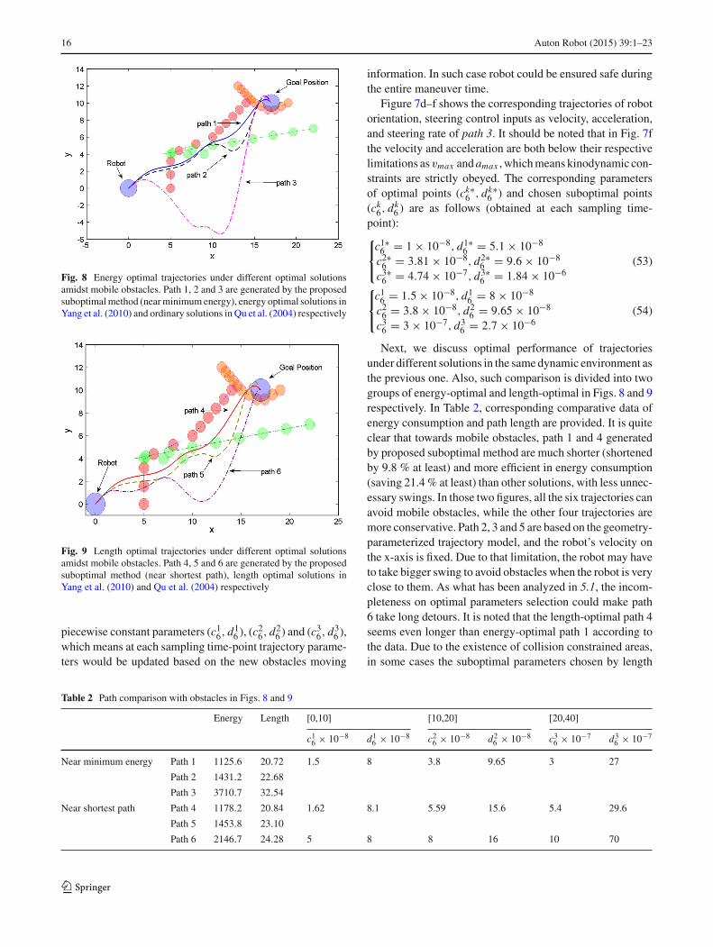
Fig. 8 Energy optimal trajectories under different optimal solutionsamidst mobile obstacles. Path 1, 2 and 3 are generated by the proposedsuboptimal method (near minimum energy), energy optimal solutions inYang et al. (2010) and ordinary solutions in Qu et al. (2004) respectively

Fig. 9 Length optimal trajectories under different optimal solutionsamidst mobile obstacles. Path 4, 5 and 6 are generated by the proposedsuboptimal method (near shortest path), length optimal solutions inYang et al. (2010) and Qu et al. (2004) respectively

piecewise constant parameters (c16, d

16 ), (c2

6, d26 ) and (c3

6, d36 ),

which means at each sampling time-point trajectory parame-ters would be updated based on the new obstacles moving

information. In such case robot could be ensured safe duringthe entire maneuver time.

Figure 7d–f shows the corresponding trajectories of robotorientation, steering control inputs as velocity, acceleration,and steering rate of path 3. It should be noted that in Fig. 7fthe velocity and acceleration are both below their respectivelimitations as vmax andamax , which means kinodynamic con-straints are strictly obeyed. The corresponding parametersof optimal points (ck∗6 , dk∗6 ) and chosen suboptimal points(ck6, d

k6 ) are as follows (obtained at each sampling time-

point):⎧⎨⎩c1∗

6 = 1 × 10−8, d1∗6 = 5.1 × 10−8

c2∗6 = 3.81 × 10−8, d2∗

6 = 9.6 × 10−8

c3∗6 = 4.74 × 10−7, d3∗

6 = 1.84 × 10−6(53)

⎧⎨⎩c1

6 = 1.5 × 10−8, d16 = 8 × 10−8

c26 = 3.8 × 10−8, d2

6 = 9.65 × 10−8

c36 = 3 × 10−7, d3

6 = 2.7 × 10−6(54)

Next, we discuss optimal performance of trajectoriesunder different solutions in the same dynamic environment asthe previous one. Also, such comparison is divided into twogroups of energy-optimal and length-optimal in Figs. 8 and 9respectively. In Table 2, corresponding comparative data ofenergy consumption and path length are provided. It is quiteclear that towards mobile obstacles, path 1 and 4 generatedby proposed suboptimal method are much shorter (shortenedby 9.8 % at least) and more efficient in energy consumption(saving 21.4 % at least) than other solutions, with less unnec-essary swings. In those two figures, all the six trajectories canavoid mobile obstacles, while the other four trajectories aremore conservative. Path 2, 3 and 5 are based on the geometry-parameterized trajectory model, and the robot’s velocity onthe x-axis is fixed. Due to that limitation, the robot may haveto take bigger swing to avoid obstacles when the robot is veryclose to them. As what has been analyzed in 5.1, the incom-pleteness on optimal parameters selection could make path6 take long detours. It is noted that the length-optimal path 4seems even longer than energy-optimal path 1 according tothe data. Due to the existence of collision constrained areas,in some cases the suboptimal parameters chosen by length

Table 2 Path comparison with obstacles in Figs. 8 and 9

Energy Length [0,10] [10,20] [20,40]

c16 × 10−8 d1

6 × 10−8 c26 × 10−8 d2

6 × 10−8 c36 × 10−7 d3

6 × 10−7

Near minimum energy Path 1 1125.6 20.72 1.5 8 3.8 9.65 3 27

Path 2 1431.2 22.68

Path 3 3710.7 32.54

Near shortest path Path 4 1178.2 20.84 1.62 8.1 5.59 15.6 5.4 29.6

Path 5 1453.8 23.10

Path 6 2146.7 24.28 5 8 8 16 10 70

123

Auton Robot (2015) 39:1–23 17

optimal solutions could be closer to energy-optimal pointsthan length-optimal points on the parameter space. There-fore, it is reasonable to find path 4 is a little longer than path1. Nevertheless, validity of our optimal principles has beenproved in example 1.

(2) Example 3 (Experiment): In order to better comparethe method in this paper with other existing results in Qu etal. (2004), Yang et al. (2005), we have to maintain the samesimulation settings in the Example 2, which results in thesmall numerical range of c6 and d6 (in the magnitude of 107).In practice, however, those values may be scaled up accordingto the given unit system as well as the setting range of robot’sdriving velocity and angular velocity. A new experiment isprovided in this part to show that in real-world settings thealgorithm is still effective and efficient to compute.

Compared to the simulation in Example 2, the experimentsettings in this part are more practical in the real-world imple-mentation, which are as follows.

– Robot kinodynamic constraints: vmax = 1.5, amax =0.5.

– Initial coordinates of the three dynamic obstacles:O1(t0) = [750, 2,000]T , O2(t0) = [1,000, 4,000]T ,O3(t0) = [2000, 500]T .

– Initial coordinates of the three static obstacles: O4 =[1,500, 300]T , O5 = [2,000, 3,500]T , O6 = [5,000,

3,800]T .– Radius of dynamic obstacles: ri = 250 (i = 1, 2, 3).

Radius of static obstacles: ri = 100 (i = 4, 5, 6).– Redefined Robot Boundary conditions: q∗

0 = (500,

500, π/16, 0, 0, 0) and q∗f = (4,500, 4,500,−π/4, 0,

600, 0).– Starting time and ending time: t0 = 0, t f = 9s.– Velocities of mobile obstacles at 0, 3 and 6 s (within each

sampling interval they remain constant):

v01 = [125,−150]T , v1

1 = [780, 850]T , v21 = [0, 0]T

v02 = [250, 0]T , v1

2 = [250, 0]T , v22 = [600,−500]T

v03 = [125, 125]T , v1

3 = [125, 125]T , v23 =

[125, 125]T– Sampling time-point: t0 = 0 s, t1 = 3 s, t2 = 6 s.– Control loop: 10 Hz

The time unit is second and the length unit is micrometer.As shown in Fig. 10, in the experiment the robot labeled

as R is desired to plan a length-optimal path that navigatesthrough three dynamic obstacles and three static obstacleswithin the given maneuver time T = 9 s. The straight lines onthe floor denote the X and Y-coordinate axes, and the movingtendency of the robot and the three dynamic obstacles are alsogiven in the figure. When any robot obstacles are detected atsampling time-point, the newest information is sent to robot

Fig. 10 Experiment scenario

R so as to update its path. Fig. 11 illustrates the mobile robotmoving in the experiment.

At the beginning, the robot computed an optimal solutionsuch as c1∗

6 = −0.05 and d1∗6 = 0.05 in order to render a

shortest path to the goal position. However, on this conditionthe robot could collide with obstacle O1 at around 3s accord-ing to the current sensed information, and hence it adjustedthe solution to an alternative suboptimal one, c1

6 = −0.08and d1

6 = 0.08, while keeping away from O1 and the sta-tic obstacle O4 sensed at 0s. When it came to 3s, the robotsensed the environment again and detected the motion changeof obstacle O1 as well as the appearance of static obstacle O5

and dynamic obstacle O3. According to the updated motioninformation of O1 and estimation, the robot would run intoO1 at around 4.5s, making the robot change the parametersagain from the inherited ones c2

6 = −0.08 and d26 = 0.08

to c26 = 0.3 and d2

6 = 1.2. Likewise, at the final samplingtime-point 6s when dynamic obstacle O1 stopped suddenlyand a new dynamic obstacle O2 rushed to the robot, it hadto replan the parameters from the ones reset at the last sam-pling moment to the new ones, c3

6 = 0.4 and d36 = 67 for the

rest of the path, thus making the robot take a relative sharpturn to avoid O2 and subsequently run a bigger detour to getaway from O1, while keeping a long distance from anothernewly detected static obstacle O6 and reaching the goal statesuccessfully and safely.

In order to compare the experiment performance with thedesired ones obtained from simulation, Fig. 12 plotted threetrajectories that are rendered by the corresponding simula-tion and the experiment. The lengths of the three paths are6,567 mm (suboptimal), 6,678 mm (designed) and approx-imately 6,700 mm (experiment). The desired velocity pro-file and the sampled velocity for the robot in simulation andthe experiment are shown in Fig. 13, both of which satisfythe kinodynamic constraints (velocity/acceleration bounds).Furthermore, in this real-world experiment of our method,the maximum running time for trajectory updating at eachsampling time-point is about 0.2 s, including the computa-tion time for solving the constrained optimization problem

123

18 Auton Robot (2015) 39:1–23

Fig. 11 Robot in experiment. a 3 s b 6 s c 9 s

500 1000 1500 2000 2500 3000 3500 4000 4500500

1000

1500

2000

2500

3000

3500

4000

4500

x(mm)

y(m

m)

Init. Pos.

Final Pos.Actual PathSuboptimal PathDesigned Path

Fig. 12 Robot actual moving path, designed path, and suboptimal pathwithout consideration of obstacles

0 1 2 3 4 5 6 7 8 90

200

400

600

800

1000

1200

Time (sec)

Vel

ocity

(m

m/s

ec)

Actual VelocityDesired Velocity

Fig. 13 Velocity profiles of the robot in experiment and in simulation

(50) using SQP or analytical solutions online. It is seen fromthe figures and data that the proposed method can work wellin real-world implementation while maintaining good effi-ciency for on-line computation.

(3) Example 4 (suboptimal solutions in highly clutteredenvironments): This part of example addresses the trajectory

Fig. 14 Robot trajectories in highly cluttered environment. Path 1 and2 are generated by length optimal solution and ’weighed optimization’in our method respectively. Path 3 are generated by length optimalsolutions in Yang et al. (2010). Path 4 is the adjusted trajectory by ourmethod under new kinodynamic constraints vmax = 1.4, amax = 0.3

generation with guaranteed combined performance understrict kinodynamic constraints in cluttered environments con-taining both static and dynamic obstacles. Redefined bound-ary conditions of the robot are q∗

0 = (0, 0, 0.53, 0, 0.6, 0)

and q∗f = (21.5, 21.5, −1.04, 0, 0.4, 0) respectively. As

shown in Fig. 14, there are seven static disc obstacles ofradius 0.5 (denoted by cyan circles with black edge). Obj1,obj2 and obj3 are three moving obstacles of radius 0.5, andthey are denoted by red, green and orange circles respec-tively. The initial kinodynamic constraints are vmax = 2.5,amax = 0.3. In Fig. 14 the maneuver time is 40s, and eachcircles of moving obstacles represent their temporal positionsof every 4 s, with arrow at initial positions indicating theirrespective moving direction.

As shown in Fig. 14, compared to path 3, path 1 and 2that generated under our method are more aggressive butstill safe in the highly cluttered environment, with obviousimprovement on path length.

Next, we consider combined optimization problem withweights ω1 = 0.5, ω2 = 0.5. Path 1 is the initial trajec-tory created according to length-optimal objective in (12), ofwhich the energy consumption and length are 3,583.0 and

123

Auton Robot (2015) 39:1–23 19

0 5 10 15 20 25 30 35 400

0.5

1

1.4

2

2.5

Time (sec)

Vel

ocity

Velocity Trajectory of Path 4Velocity Trajectory of Path 3Velocity Trajectory of path 1

Fig. 15 Robot velocity trajectories of the paths in Fig. 14. Blue dashedcurve andmagenta dash-dotted curve represent trajectories under origi-nal velocity limitation of 2.5.Red solid curve represents trajectory undernew velocity limitation of 1.4 (Color figure online)

33.51. By specifying ω1 = 0.5, ω2 = 0.5 into the combinedperformance index (14), path 2 is rendered with updated opti-mal performance of 3,397.7/33.87 in energy consumptionand path length. Since the performance evaluation on energyand length are more balanced, compared to path 1, the lengthof path 2 is sacrificed a bit for the improvement on energyconsumption.

Besides, to highlight flexibility of our method, new kin-odynamic constraints are employed in this example(takingnew velocity limitation for instance). With the same environ-ment in Fig. 14, velocity constraint of robot is changed fromvmax = 2.5 to vmax = 1.4, making it impossible for robot toeasily outrun the moving obstacles. The initial velocity trajec-tory of path 1 and 3 in Fig. 14 are shown in Fig. 15. Althoughrobot motions on both of the two trajectories satisfy the orig-inal limitation of 2.5, they violate the new one. In order toreplan a feasible path under such updated constraints usingour method, we investigate the selection of new parameterpoints on parameter space in Figs. 16 and 17. It is noted thatthe chosen suboptimal point in Fig. 16 is no longer coveredby the solution area (restrained area) in Fig. 17, which meansthe previous trajectory will not satisfy the present limitation.So, we choose an alternative suboptimal point in Fig. 17 suchthat the solution space wholly cover the selected point. Theupdated velocity trajectory of such path is shown by red solidcurve in Fig. 15, and updated path is given by red solid curvein Fig. 14. These results show that feasible solutions can alsobe found by our method to plan a qualified path in front ofupdated kinodynamic constraints.

Remark 10 It should be noted that although data of theenergy consumption and path length in Table 1 and 2 don’tseem to diverge much in absolute value, the percentage ofthose difference could still reveal the effects. In real world

−1.5 −1 −0.5 0 0.5 1 1.5 2

x 10−7

−5

0

5

10

15

20

25x 10

−8

c6

d6

Primitive Length−optimal point for Path 1 and 4

Sub−Length−optimalpoint for Path 1

Fig. 16 Solution space in the parameter space under initial velocitylimitation of 2.5. Red circle sets represent corresponding feasible areasmapped from analytic inequations (4). Blue circle sets represent col-lision areas with static and dynamic obstacles, which is mapped from(39). Magenta point is the chosen suboptimal solution of trajectoryparameters c6 and d6 (Color figure online)

−5 0 5 10 15

x 10−8

−5

0

5

10

x 10−8

c6

d6

Primitive Length−optimal point for Path 1 and 4

Sub−Length−optimal point for Path 4

Fig. 17 Solution space in the parameter space under updated velocitylimitation of 1.4. Red circle sets represent corresponding feasible areasmapped from analytic inequations (4). Blue circle sets represent col-lision areas with static and dynamic obstacles, which is mapped from(39). Magenta point is the re-chosen suboptimal solution of trajectoryparameters c6 and d6 (Color figure online)

applications, the unit used could always be much larger askilometer of length, rather than standard meter in this simu-lation section, which can better prove the excellence of theproposed method. �

5.3 Adjustment towards non-solution situation

This section considers trajectory re-generation towards non-solution situation to improve the completeness of our method.Since solution space in parameter space such as those inFigs. 16 and 17 may not always exist, what happens whenthe robot cannot physically find a feasible solution? As wehave discussed in previous part, proper adjustment of termi-

123

20 Auton Robot (2015) 39:1–23

−5 0 5 10 15

x 10−8

−8

−6

−4

−2

0

2

4

6

8

10

12x 10

−8

c6

d6

Primitive Length−optimal point

No solutions available under given terminal time tf=40s

Fig. 18 Solution space in the parameter space becomes null understrict velocity limitation of 1.2 with original terminal time t f =40s

−3 −2 −1 0 1 2 3 4 5 6 7

x 10−8

−4

−3

−2

−1

0

1

2

3

4

5x 10

−8

c6

d6

Length−optimal point

Chosen sub−optimal point

Feasible Solutions Areas under modified terminal time tf=50s

Fig. 19 Solution space in the parameter space reappears after prolong-ing the terminal time t f from 40 to 50 s

nal time can be employed in our method to find feasible solu-tions unless all possible passages are blocked by obstacles.This case is investigated by further limiting the velocity con-straint inExample 4 from 1.4 to 1.2, with the same settings ofother environment parameters in Fig. 14. Due to such strictlyimposed constraint, the initial solution space in Fig. 17 ceaseto exist, as shown in Fig. 18.

Since the non-solution situation in this case is caused onlyby strict velocity constraint, we prolong the terminal time t fto 50s. It is reasonable in real-world to extend maneuver timefor low speed navigation of mobile robots. Then, it is notedthat the feasible solution space empty in Fig. 18 reappearsin Fig. 19. The following selection of parameter points issimple as ordinary suboptimal process of our method. Asthe magenta point chosen in Fig. 19, a feasible suboptimalpoint is found to generate new trajectories. The comparisonof paths and velocity trajectories before and after such adjust-ment are shown in Figs. 20 and 21. After adjustment, robotcan still generate a feasible collision-free path to achieve the

Fig. 20 Path comparison in cluttered environment. Blue dashed path1 is generated under original terminal time t f =40s. Red solid path 2 isgenerated under adjusted terminal time t f =50s (Color figure online)

0 5 10 15 20 25 30 35 40 45 500.2

0.4

0.6

0.8

1

1.2

1.4

1.6

Time (sec)

Vel

ocity

Velocity Trajectory of Path 2Velocity Trajectory of Path 1

Fig. 21 Velocity trajectories comparison of paths in Fig. 20. Bluedashed curve corresponds to path 1 under original terminal time. Redsolid curve corresponds to path 2 under adjusted terminal time (Colorfigure online)

original goal, while well satisfying the given strict kinody-namic constraints. This is an example where non-solutionsituation appears, our approach could still try to find an alter-native way to complete the tasks. It should be noted that thesolvable or unsolvable situations in Figs. 19 and 18 are foundbefore executing, and robot can determine whether to adjustterminal time in advance to guarantee the feasibility of tra-jectories once generated, which is good for on-line planning.Nonetheless, as discussed in the part of Algorithm Complete-ness and Stability, it cannot be ensured that the solutions willalways be found under all circumstances.

6 Conclusion

This paper presents a novel analytical method to solve com-bined optimization trajectory generation problem for mobile

123

Auton Robot (2015) 39:1–23 21

robots with kinodynamic constraints in the presence of mov-ing obstacles. Analytical suboptimal solutions that integratetwo different weighed optimal performance indices can flex-ibly satisfy various optimal requirements. By explicitly con-sidering redefined higher dimensional boundary conditionsas well as robot kinodynamic constraints and collision avoid-ance criteria, the constrained optimal trajectory generationproblem was recast as a constrained minimum distance prob-lem on a 2D parameter space with straightforward geometricimplications that can be well handled by simple on-line com-putation with analytical results or SQP method. The analyti-cal suboptimal solutions could automatically detect unsolv-able situations and make remedies to make the problem solv-able. Simulation and experiment results have verified the effi-ciency and effectiveness of the proposed method in dealingwith local dynamic environments. Further works include anextension of the proposed approach to other global search-based algorithm in order to deal with highly dense 2D/3Denvironment and solve the issues as lack of completenessand stability. Another issue is to further improve the rig-orousness of the method by quantify the exact amount oftime to be extended in order for the robot to retain feasiblepaths.

Acknowledgments The authors would like to acknowledge that thiswork was partially supported by the National Natural Science Foun-dation of China (Grant No. 61379111, 61402538 and 61202342) andSpecialized Research Fund for the Doctoral Program of Higher Educa-tion (20110162110042).

References

Balkcom, D. J., & Mason, M. T. (2002). Time optimal trajectoriesfor bounded velocity differential drive vehicles. The InternationalJournal of Robotics Research (IJRR), 21, 199–217.

Barraquand, J., & Latombe, J. C. (1991). Nonholonomic multibodymobile robots: Controllability and motion planning in the presenceof obstacles.Proceedings of the IEEE International Conference onRobotics and Automation (ICRA), 3, 2328–2335.

Bhattacharya, S., Likhachev, M., & Kumar, V. (2012). Topological con-straints in search-based robot path planning. Autonomous Robots,33(3), 273–290.

Bicchi, A., Casalino, G., & Santilli, C. (1995). Planning shortestbounded-curvature paths for a class of nonholonomic vehiclesamong obstacles. Proceedings of the IEEE International Confer-ence on Robotics and Automation (ICRA), 2, 1349–1354.

Bonnans, J.-F., et al. (2006). Numerical optimization: Theoretical andpractical aspects. Heidelberg: Springer.

Borenstein, J., & Koren, Y. (1991). The vector field histogram-fastobstacle avoidance for mobile robots. IEEE Transactions onRobotics and Automation, 7, 278–288.

Cheng, P., Frazzoli, E., & LaValle, S. (2008). Improving the perfor-mance of sampling-based motion planning with symmetry-basedgap reduction. IEEE Transactions on Robotics, 24, 488–494.

Divelbiss, A. W., & Wen, J. T. (1997). A path space approach to non-holonomic motion planning in the presence of obstacles. IEEETransactions on Robotics and Automation, 13, 443–451.

Dong, W., & Guo, Y. (2005). New trajectory generation methods fornonholonomic mobile robots. Proceedings of the internationalsymposium on collaborative technologies and systems, pp. 353–358.

Duleba, I., & Sasiadek, J. Z. (2003). Nonholonomic motion planningbased on Newton algorithm with energy optimization. IEEETrans-actions on Control Systems Technology, 11, 355–363.

Fiorini, P., & Shiller, Z. (1993). Motion planning in dynamic envi-ronments using the relative velocity paradigm. Proceedings ofthe IEEE International Conference on Robotics and Automation(ICRA), 1, 560–565.

Fliess, M., LeVine, J., Martin, P., & Rouchon, P. (1995). Flatness anddefect of non-linear systems: Introductory theory and examples.International Journal of Control, 61, 1327–1361.

Guo, Y., & Tang, T. (2008). Optimal trajectory generation for nonholo-nomic robots in dynamic environments. Proceedings of the IEEEinternational conference on robotics and automation (ICRA), pp.2552–2557.

Guo, Y., Li, Y., & Sheng, W. (2007). Global trajectory generation fornonholonomic robots in dynamic environments. Proceedings ofthe IEEE international conference on robotics and automation(ICRA), pp. 1324–1329.

Hashim, S., & Tien-Fu, L. (2009). A new strategy in dynamic time-dependent motion planning for nonholonomic mobile robots. IEEEinternational conference on robotics and biomimetics (ROBIO),pp. 1692–1697.

Howard, T. M., & Kelly, A. (2007). Optimal rough terrain trajectorygeneration for wheeled mobile robots. International Journal ofRobotics Research (IJRR), 26(2), 141–166.

John, S., et al. (2014). Motion planning with sequential convex opti-mization and convex collision checking. The International Journalof Robotics Research, 33(9), 1251–1270.

Karaman, S., & Frazzoli, E. (2010). Optimal kinodynamic motion plan-ning using incremental sampling-based methods. In: 49th IEEEconference on decision and control (CDC), pp. 7681–7687.

Kim, J. O., & Khosla, P. K. (1992). Real-time obstacle avoidance usingharmonic potential functions. IEEE Transactions on Robotics andAutomation, 8, 338–349.

Kindel, R., Hsu, D., Latombe, J. C., & Rock, S. (2000). Kinody-namic motion planning amidst moving obstacles. Proceedings ofthe IEEE International Conference on Robotics and Automation(ICRA), 1, 537–543.

Koenig, Sven, & Likhachev, Maxim. (2002). D* Lite.Proceedings of theeighteenth national conference on artificial intelligence (AAAI),pp. 476–483.

Kushleyev, A., & Likhachev, M. (2009). Time-bounded lattice for effi-cient planning in dynamic environments. Proceedings of the IEEEinternational conference on robotics and automation (ICRA), pp.1662–1668.

Ladd, A. M., & Kavraki, L. E. (2004). Measure theoretic analysis ofprobabilistic path planning. IEEE Transactions on Robotics andAutomation, 20, 229–242.

LaValle, S. M., & Kuffner, J. J, Jr. (1999). Randomized kinodynamicplanning. Proceedings of the IEEE International Conference onRobotics and Automation (ICRA), 1, 473–479.

LaValle, S. M. (2006). Planning algorithms. Cambridge: CambridgeUniversity Press.

Li, Z. X., & Canny, J. (1992). Nonholonomic motion planning, Dor-drecht. The Netherlands: Kluwer.

Likhachev, M., & Ferguson, D. (2009). Planning long dynamically-feasible maneuvers for autonomous vehicles. International Jour-nal of Robotics Research (IJRR), 28(8), 933–945.

Liu, S., & Sun, D. (2011). Optimal motion planning of a mobile robotwith minimum energy consumption. IEEE/ASME internationalconference on advanced intelligent mechatronics (AIM), pp. 43–48.

123

22 Auton Robot (2015) 39:1–23

De Luca, A., Oriolo, G., & Samson, C. (1998). Feedback control of anonholonomic car-like robot.RobotMotion Planning andControl,229, 171–253.

Lvine, J. (2009). Analysis and control of nonlinear systems: A flatness-based approach. Berlin: Springer.

Morales, J. L., Nocedal, J., Wu, Y. (2011). A sequential quadratic pro-gramming algorithm with an additional equality constrained phase.IMA Journal of Numerical Analysis, drq037.

Murray, R. M., & Sastry, S. S. (1993). Nonholonomic motion plan-ning: Steering using sinusoids. IEEE Transactions on AutomaticControl, 38, 700–716.

Narayanan, V., Phillips, M., & Likhachev, M. (2012). Anytime safeinterval path planning for dynamic environments. Proceedings ofthe IEEE/RSJ international conference on intelligent robots andsystems (IROS), pp. 4708–4715.

Pivtoraiko, M., Knepper, R. A., & Kelly, A. (2009). Differentially con-strained mobile robot motion planning in state lattices. Journal ofField Robotics (JFR), 26(3), 308–333.

Qu, Z., Wang, J., & Plaisted, C. E. (2004). A new analytical solutionto mobile robot trajectory generation in the presence of movingobstacles. IEEE Transactions on Robotics, 20, 978–993.

Reister, D. B., & Pin, F. G. (1994). Time-optimal trajectories for mobilerobots with two independently driven wheels. The InternationalJournal of Robotics Research (IJRR), 13, 38–54.

Shiller, Z., Gal, O., & Raz, A. (2011). Adaptive time horizon for on-lineavoidance in dynamic environments.Proceedings of the IEEE/RSJinternational conference on intelligent robots and systems (IROS),pp. 3539–3544.

Shiller, Z., Large, F., & Sekhavat, S. (2001). Motion planning in dynamicenvironments: Obstacles moving along arbitrary trajectories. Pro-ceedings of the IEEE International Conference on Robotics andAutomation (ICRA), 4, 3716–3721.

Tilbury, D., & Murray, R. M. (1995). Trajectory generation for the N-trailer problem using Goursat normal form. IEEE Transactions onAutomatic Control, 40, 802–819.

Ucan, X. I., & Kavraki, L. E. (2012). A sampling-based tree planner forsystems with complex dynamics. IEEE Transactions on Robotics,28, 116–131.

van den Berg, J., & Overmars, M. (2007). Kinodynamic motion plan-ning on roadmaps in dynamic environments. Proceedings of theIEEE/RSJ international conference on intelligent robots and sys-tems (IROS), pp. 4253–4258.

Wu, A., & How, J. P. (2012). Guaranteed infinite horizon avoidanceof unpredictable, dynamically constrained obstacles. AutonomousRobots, 32(3), 227–242.

Yang, J., Daoui, A., Qu, Z., Wang, J., & Hull, R. A. (2005). An opti-mal and real-time solution to parameterized mobile robot trajecto-ries in the presence of moving obstacles. Proceedings of the IEEEinternational conference on robotics and automation (ICRA), pp.4412–4417.

Yang, J., Qu, Z., Wang, J., & Conrad, K. (2010). Comparison of optimalsolutions to real-time path planning for a mobile vehicle. IEEETransactions on Systems, Man and Cybernetics, Part A: Systemsand Humans, 40, 721–731.

Yuan, H., & Shim, T. (2011). Model based real-time collision-freemotion planning for mobile robots in unknown dynamic envi-ronments. In: 14th international IEEE conference on intelligenttransportation systems (ITSC), pp. 416–421.

Jun Peng is a Professor inSchool of Information Science& Engineering at the CentralSouth University, China. Herresearch interests include coop-erative control; Multi-agent sys-tems and wireless communica-tions. She received her B.S.degree from Xiangtan Univer-sity and the MSc degree fromNational University of DefenseTechnology, China, in 1987 and1990, respectively. She receivedher PhD degree from CentralSouth University in 2005. In

April, 1990, she joined the staff of Central South University. From2006 to 2007, she was with School of Electrical and Computer Scienceof University of Central Florida, USA, as a visiting scholar. She is aMember of IEEE.

WenhaoLuo received the B.Engdegree in Measurement & Con-trol Technology and Instrumentsfrom Central South University,China, in 2012. He is cur-rently pursuing the M. S. Degreein Robotics at Robotics Insti-tute, Carnegie Mellon Univer-sity, USA where he is also aresearch assistant. Before that,he was a research assistant andPh.D. candidate in Control Sci-ence and Engineering in theDepartment of Automation atShanghai Jiao Tong University,

China, from 2012 to 2014. His research interests are in the areas ofmotion planning, multi-agent systems and control theory.

Weirong Liu received his B.S.,M.S degrees in the School ofInformation Science and Engi-neering, Central South Univer-sity, and received his Ph.D.degrees in the Laboratory ofComplex Systems & IntelligenceScience, Institute of Automa-tion, Chinese Academy of Sci-ences. Currently, he is an asso-ciate professor of the School ofInformation Science and Engi-neering, Central South Univer-sity. His special fields of inter-est include robot control, cooper-ative control, networked systemcontrol and multi-agent system.

123

Auton Robot (2015) 39:1–23 23

Wentao Yu received the B.Sdegree and M.E degree fromCentral South University, Chang-sha, China in 2004 and 2008respectively. She is currentlypursuing the Ph.D. degree inSchool of Information Scienceand Engineering, Central SouthUniversity. Her research focuseson cooperative navigation ofautonomous vehicles. Specifi-cally she is investigating cooper-ative path planning strategies fora team of autonomous vehiclesunder dynamic constraints.

Jing Wang received the Ph.D.in control theory and controlengineering from Central SouthUniversity, China, in 1997. Hewas a Postdoctoral Research Fel-low at the Institute of Comput-ing Technology, Chinese Acad-emy of Sciences, from 1997to 1999, and at Department ofElectrical and Computer Engi-neering, National University ofSingapore, from 1999 to 2002.From 2002 to 2007, He was withSchool of Electrical Engineeringand Computer Science of Univer-

sity of Central Florida as a Research Assistant Professor. From 2007 to2014, he was with the Department of Computer Engineering, Bethune-Cookman University, first as an Assistant Professor and then AssociateProfessor. Since August 2014, he joined in the Department of Electri-cal and Computer Engineering, Bradley University, Peoria, IL, as anAssistant Professor. He is a Senior Member of IEEE.

123