A Study on Design of Prestressed Post-Tensioned Girder by Morice ...

International Journal of Innovative Research in Advanced Engineering (IJIRAE) ISSN: 2349-2163 Issue 5, Volume 2 (May 2015) www.ijirae.com

___________________________________________________________________________________________________ © 2014-15, IJIRAE- All Rights Reserved Page -160

A Study on Design of Prestressed Post-Tensioned Girder by Morice-Little Method

D.Gouse Peera1 Mahendrakar Kiran Kumar2 Konge Praveen Kumar3

1(Associate Professor, Civil Engineering, BITS Adoni, Kurnool District, Andhra Pradesh, India) 2(M.Tech student, Civil Engineering, BITS Adoni, Kurnool District, Andhra Pradesh, India) 3(M.Tech student, Civil Engineering, BITS Adoni, Kurnool District, Andhra Pradesh, India)

ABSTRACT: Prestressed concrete is useful for big spans and rapid completion of construction works. Prestressed concrete mainly used in buildings, bridges and towers. In this paper the design of prestressed girder elements are discussed, various methods and their suitability for the design are discussed, mainly concentrated on Morice-Little method. In our analysis, the effective width is divided into eight equal segments, the nine boundaries of which are known as the standard positions, the loadings and deflections at these nine standard positions are considered and all deflections are related to the average deflection. The design of a girder for a bridge taken as an example and results are provided with neat sketches. Girders may be post-tensioned or pre-tensioned and also precast or cast-in-situ. With this manuscript any structural engineer can get an succinct idea about how Morice-Little method implemented in the design of a prestressed post-tensioned girder.

Keywords: Girder, Morrice-Little, Prestressed concrete, Cross beam.

I. INTRODUCTION

There are various methods for design of girders of post-tensioned prestressed concrete road bridges. In India Indian Road Congress publishes codes and specifications for design. Usually, concrete of grade M40 is used for post-tensioned prestressed girders. Before start design dimensions are assumed based on experience. The design involves calculation of the section properties, dead load moments, live load moments, magnitude and location of the prestressing force, profile of the tendons, shear stresses at different sections. Finally design of end block and cross beams.

II. DESIGN METHODS FOR CONCRETE BRIDGES

In order to compute the bending moment due to live load in a girder and slab bridge, the distribution of the live loads among the longitudinal girders has to be determined. When there are only two longitudinal girders, the reactions on the longitudinal can be found by assuming the supports of the deck slab as unyielding. With three or more longitudinal girders, the load distribution is estimated using any one of the rational methods. Three of these are Courbon’s method, Hendry-Jaegar method, Morice and little version of Guyon and Massonnet method.

2.1. Courbon’s Method

According to Courbon’s method, the reaction Ri of the cross beam on any girder I of a typical bridge consisting of multiple parallel beams is computed assuming a linear variation of deflection in the transverse direction. The deflection will be maximum on the exterior girder on the side of the eccentric load (or c.g. of loads if there is system of concentrated loads) and minimum on the other exterior girder. The reaction R¡ is then given by (or) where p, Li, e, are di total live load, Moment of inertia of longitudinal girder i, eccentricity of the live load (or C.G. of loads in case of multiple loads) and distance of girder i from the axis of the bridge.When the intermediate and the end longitudinal girders have the same moment of inertia, the quantity li in the second term within brackets of above equation gets cancelled and the term outside the bracket now reduces to p/n, where n is the number of longitudinal girders. This reduces the amount of computation considerably. In view of the simplicity in calculations, this method is very popular. Courbon’s method is applicable only when the following conditions are satisfied. The ratio of span to width is greater than 2 but less than 4. The longitudinal beams are interconnected by symmetrically spaced cross girders of adequate stiffness. The cross girders extend to a depth of at least 0.75 of the depth of the longitudinal girder. These conditions are usually satisfied for majority of modern T-beam bridges.

3.2. Hendry-Jaegar Method Hendry and Jaegar assume that the cross beams can be replaced in the analysis by a uniform continuous transverse

medium of equivalent stiffness. According to this method, the distribution of loading in an inter connected bridge deck system depends on the following three dimensionless parameters.

A = 12 / π4 (L / h)3 n ElT / EI, F = π2 / 2n (h / L) CJ / EIT, C = EI1 / EI2

Here L, h and n are span of the bridge, spacing of longitudinal girders and n number of cross beams. EI, CJ = Flexural and torsional rigidities, respectively, of one longitudinal girder. EI1, EI2 = Flexural rigidities of the outer and inner longitudinal girders, where these are different EIT = Flexural rigidity of one cross beam.



In case of beam and slab bridge without cross beams, n and EIT in above equations is to be replaced by L and EIT

where the latter gives the total flexural rigidity of the slab deck. Normally, for reinforced concrete T-beam bridges, the flexural rigidities of the outer and inner longitudinal girders will be nearly equal. The parameter A is the most important of the above three parameters. it is a function of the ratio of transverse to longitudinal flexural rigidity. The second parameter F is a measure of the relative torsional rigidity of the longitudinal and is difficult to determine accurately, due to uncertainties surrounding the CJ values for practical girder sections. For T-beam bridges having three or four longitudinal with a number of cross beams, it is usually permissible to employ the distribution coefficients for F= ∞. The torsional rigidity of the transverse system is neglected in the analysis. Graphs giving the values of the distribution coefficients (m) for different conditions of number of longitudinal (two to six) and two extreme values of F, i.e. zero and infinity. Coefficients for intermediate values of F may be obtained by interpolation from equation 푀 = 푚 + (푚∞ −݉0F3ܣ+Fܣ where MF is the required distribution coefficient and mo and m∞ are respectively the coefficients for F = 0 and F = ∞.

3.3. Morice and little method

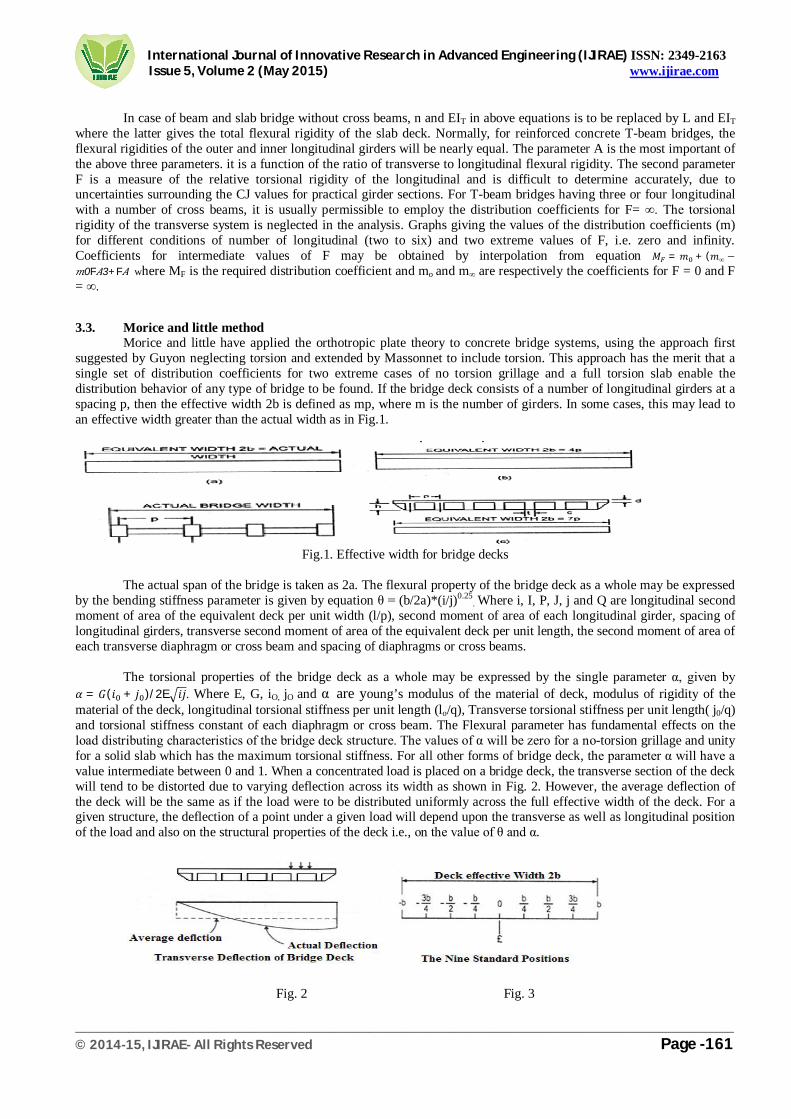
Morice and little have applied the orthotropic plate theory to concrete bridge systems, using the approach first suggested by Guyon neglecting torsion and extended by Massonnet to include torsion. This approach has the merit that a single set of distribution coefficients for two extreme cases of no torsion grillage and a full torsion slab enable the distribution behavior of any type of bridge to be found. If the bridge deck consists of a number of longitudinal girders at a spacing p, then the effective width 2b is defined as mp, where m is the number of girders. In some cases, this may lead to an effective width greater than the actual width as in Fig.1.

Fig.1. Effective width for bridge decks The actual span of the bridge is taken as 2a. The flexural property of the bridge deck as a whole may be expressed

by the bending stiffness parameter is given by equation θ = (b/2a)*(i/j)0.25. Where i, I, P, J, j and Q are longitudinal second

moment of area of the equivalent deck per unit width (l/p), second moment of area of each longitudinal girder, spacing of longitudinal girders, transverse second moment of area of the equivalent deck per unit length, the second moment of area of each transverse diaphragm or cross beam and spacing of diaphragms or cross beams.

The torsional properties of the bridge deck as a whole may be expressed by the single parameter α, given by

훼 = 퐺(푖 + 푗 )/2E 푖푗. Where E, G, iO, jO and α are young’s modulus of the material of deck, modulus of rigidity of the material of the deck, longitudinal torsional stiffness per unit length (lo/q), Transverse torsional stiffness per unit length( j0/q) and torsional stiffness constant of each diaphragm or cross beam. The Flexural parameter has fundamental effects on the load distributing characteristics of the bridge deck structure. The values of α will be zero for a no-torsion grillage and unity for a solid slab which has the maximum torsional stiffness. For all other forms of bridge deck, the parameter α will have a value intermediate between 0 and 1. When a concentrated load is placed on a bridge deck, the transverse section of the deck will tend to be distorted due to varying deflection across its width as shown in Fig. 2. However, the average deflection of the deck will be the same as if the load were to be distributed uniformly across the full effective width of the deck. For a given structure, the deflection of a point under a given load will depend upon the transverse as well as longitudinal position of the load and also on the structural properties of the deck i.e., on the value of θ and α.

Fig. 2 Fig. 3



In the analysis, the effective width is divided into eight equal segments, the nine boundaries of which are known as the standard positions as shown in Fig. 3. The loadings and deflections at these nine standard positions are considered and all deflections are related to the average deflection. The actual deflection at each of these nine standard positions will be given by an arithmetical coefficient, called distribution coefficient and denoted by the symbol K, multiplied by the average deflection produced by the load distributed uniformly across the entire effective width. We can find values from Morice-Little curves such as transverse moment coefficients µ0 at reference station 0, distribution coefficient K1 at reference station b/2, b/4, 3b/4, distribution coefficients K1 at reference station 0, distribution coefficients K0 at reference station b, b/2, b/4, 3b/4, distribution coefficients K0 at reference station 0, large range distribution coefficients K0. The curves give the distribution coefficient at each standard reference point for a load applied at any of the nine standard positions for a bridge deck with zero torsional stiffness. The value of K for α equal to zero is denoted by K0 and α equal to 1is denoted by K1. For an intermediate values of α, the distribution coefficient can be obtained from the interpolation relationship given in equation Kα = k0 + (k1-k0)√α where Kα, K1 and K0 are the distribution coefficient for the actual value of α, distribution coefficient for α equal to zero, distribution coefficient for equal to 1.

The above distribution coefficients have been derived for deflections. However these may also be applied for

longitudinal bending moments and, therefore to longitudinal bending stresses. Since the mathematical analysis used for the preparation of the design curves used only the first term of the harmonic series, the bending moment and stress under a concentrated load are to be increased by 10 percent for design. Transverse bending moments are caused by the unequal deflections across a transverse section due to the application of a concentrated load. The transverse bending moment, My is given by equation. 푀 = ∑ 휇 푟 푏 sin∞ , where µnθ and rn are distribution coefficient analogous to K for deflection and the nth coefficient of the Fourier series representing the longitudinal position of the load.

In practice, it is normally adequate to consider only five terms of the series in equation, which would then reduce

to equation My = (µθr1 - µ3θr3 + µ5θr5), For the case of a concentrated load W at a distance u from the left support, rn is given by equation 푟 = 푋푠푖푛 , the equation gets modified to equation 푀 = µØsin −µ Ø푠푖푛 + µ Ø the greatest transverse moments occur with a concentrated load, when it is nearest to the longitudinal axis. In bridges with no central islands, it is generally adequate to use the curves for the standard position only. The curves for µθ and µ1 for the standard positions 0 for α equal to zero and unity, respectively, are find from curves. The values of µ corresponding to any intermediate values of α can be evaluated using the interpolation relation in equationµ = µ + (µ − µ )√훼.

III. DESIGN PROCEDURE

3.1. Design of simply supported decks Dimensions are assumed based on experience, such as the overall depth is usually about 75-85mm for every meter

of span. The thickness of deck slab is about 150-200mm with transverse prestressing and about 200-250mm in composite construction. The minimum thickness of web of precast girder is 150mm plus the diameter of cable duct. The bottom width of the precast beam may vary from 500-800mm. Compute the section properties based on the full section without deducting for the cable ducts. Compute dead load moments, live load moments & corresponding stresses for girders, but the live load moments is to be taken for the severest applicable condition of loading. Determine the magnitude and location of the prestressing force at the point of maximum moment. The prestressing force must meet two conditions, viz. it must provide sufficient compressive stress to offset the tensile stresses which will be caused by the bending moments, it must not induce either tensile or compressive stresses which are in excess of those permitted by the specifications. Select the prestressing tendons to be used and work out the details of their locations in the member. Avoid grouping of tendons, as grouting of some after first stage ducts if the sheaths are not leak proof. If unavoidable, use group of two cables on vertically above the other. Allow a minimum clear cover of 50 mm to the cables. Ensure that a normal needle vibrator can reach almost to the bottom row of cables while placing the concrete for the girder. Determine the profile of the tendons, and check the stresses at critical points along the member under initial and final conditions such as initial prestress plus dead load only & final prestress plus full design load.

The profile of the tendons may be parabolic for the full length from one anchorage to the other. Alternatively, a tendon may have a central straight portion with parabolic profile at either end. The draping of the tendons helps to bring the stresses in concrete at every section within the permissible range. This also serves to reduce the net shear at any section. While it is possible to anchor some of the draped tendons on the deck surface, recent practice is to avoid such deck-anchored tendons. If necessary, the sizes of the tendons and the webs are suitably increased and the tendons are anchored at the ends of the girder in the end blocks. The moment due to applied load is zero at the end of the girder. The anchorages should be spread evenly over as large an area as possible. At the ends of the girders, the centre of gravity of steel should ideally coincide with the total mass passing point of concrete. At every other section, the centre of gravity of steel must lie in such a position that the internal moments of resistance balance the applied moments, so that the concrete stresses lie within the permissible range. Check the ultimate strength to ensure that the requirements of IRC:18 are met. The ultimate load under moderate exposure condition is to be taken as 1.25 G+2G+2.5Q where G, SG and Q denote permanent load, superimposed load and live load including impact, respectively.



For severe exposure condition, the ultimate load is to be taken as 1.5G+2SG+2.5Q. Work out the shear stresses at different sections and design the shear reinforcement. Check the stresses at the jacking end due to cable forces and these should be within permissible limits. While designing the end block, the end block should be rectangular in section of width equal to the bottom flange of the girder. Ensure the adequate un-tensioned reinforcement is provided as specified in section 12 of IRC: 18. The bars of such reinforcement should have a diameter not less than 8 mm and the spacing not more than 200 mm. The reinforcement in the vertical direction should be not less than 0.18 per cent of the plan area of web/bulb of the girder. The longitudinal reinforcement should be not less than 0.15 per cent of the cross sectional area. The spacing should be uniform to the extent possible. For the designing the deck slab, any rational method may be used. The design may follow the procedure as for deck slab for R.C.T-beam bridge. For the design of cross beams, any rational method may be used. In case of end cross beam, provision should be made for possible jacking for replacement of bearings. The length of the end block should be about one-half of the depth of the girder, but not less than 600 mm or its width. The thickness of the web of the girder towards the end block should be achieved gradually with a splay in plan of not more than 1 in 4. The portion housing the anchorages should as far as possible be precast. The concentrated force at an anchorage causes bursting tensile force and spalling tensile forces in the end block. The bursting tensile forces is estimated from tabular values given in IRC:18 as a function of the forces in the tendons and the ratio of the loaded width to the total width at the anchorage without overlap. The stress is maximum at a distance of about half the width of the end block behind the anchorage. In rectangular end blocks, the bursting tensile force should be assessed in two principle directions. The reinforcement for the bursting tensile forces should be provided in the region 0.1 b2 to b2 behind the anchorage, where b2 is the side of effective anchor area. Spalling tensile forces occur immediately behind the anchorage and the anchorage and the end face of the anchorage zone. The reinforcement is provided by two layers of meshes of small diameter. Also the end face of the anchorage zone is continually reinforced to prevent edge spalling, the reinforcement being placed as close to the end as possible. Additionally, spiral reinforcement is provided for embedded anchors.

IV. DISCUSSION OF RESULTS

4.1. SPECIFICATIONS 4.1.1. Details of The Bridge Length of bridge 2a is 25 m, width of bridge 2b is 8.7 m, number of main girders are 5, number of cross beams 6, main girder spacing p is 1.74 m, cross beam spacing q is 5m and carriage way 7.5 m 4.1.2. Basic of Calculations Live load as per IRC Class AA tracked loading and Regulation as per IRC: 5; IRC: 6; IRC: 18; IRC: 21. 4.1.3. Materials Tensioned Steel as high tensile steel 5mm, 7mm and 8 mm dia. wires conforming to clause 4.3.2 of IS: 1342-1960. Ultimate tensile strength is 1600 MPa for 5 mm wires and 1500 MPa for 7 mm and 8 mm wires. Modulus of Elasticity 2.1×105 MPa, un-tensioned steel: HYSD bars Grade Fe415 conforming to IS: 1786. Controlled concrete grade of M40, permissible stresses as per section 7 of IRC: 18, maximum permanent compressive stress and temporary compressive stress at transfer are 13.2 MPa and 0.50fcj respectively where fcj being the concrete strength at transfer, permissible permanent tensile stress and permissible temporary flexural tensile stress 0 and 0.05fci and modulus of Elasticity Ec 5000√fck i.e,. 31620 MPa. 4.2. PRELIMINARY DIMENSIONS Overall depth required is to be taken as 70 to 85 mm per 1 m span i.e,. 1750mm, width of bridge is 8.7 m in which 5 longitudinal girders are provided each one having assumed depth of 1000 mm. Overall depth of girder 1000 mm, flange thickness is 200 mm at free end and, 300 mm at fixed, thickness of web is 200 mm, spacing of main girder 1.74 m and spacing of cross beam is 5 m. The cross section of bridge at end and mid span as shown in fig 4 and 5.

Fig.4 Fig.5



4.3. DESIGN OF POST-TENSIONED PRESTRESSED CONCRETE GIRDER 4.3.1. Section Properties No deductions for holes are made in calculating the properties of girder and cross beam. This is permissible, since no allowance for the transformed area of the prestressing tendons is included in the calculation. The cross-sectional dimensions of a precast longitudinal girder can be obtained from fig. The section properties are then computed as below. Here yt and yb denote the distance to extreme fiber of concrete at top and bottom respectively, from the neutral axis. ‘I’ denoted by the second moment of area. For design purpose we are taken only one main girder cross section as in Fig.6. The section converted into rectangular flanges for simplification as shown in Fig. 7.

Fig.6 Fig.7

Fig.8

Section properties of girder like Section modules w.r.t to extreme fibers i.e,. Zt,Zb & torsional stiffness at mid span Io are to be determined by means of calculating the area of cross section a, center of gravity y, neutral axis depth from bottom yb and top yt, second moment of area of section at centroidal axis Ica etc for the cross section of main girder at mid span section, end section and cross beam at mid span section are calculated. The respective fig is shown in Fig 6, 7 & 8.

4.3.2. Distribution coefficients by Morice-little method

The distributed longitudinal stiffness coefficient i (ratio of second moment of area of section for main girder I and spacing of main girder p), distributed transverse stiffness coefficient j (the ratio of second moment of area of section for cross beam J and Spacing of cross beam q), bending stiffness parameter θ, torsional Stiffness Parameter α, Distributed Transverse Torsional Stiffness jo (ratio of torsional stiffness of cross beam Jo and cross beam spacing q), Distributed Longitudinal Torsional Stiffness io (ratio of torsional stiffness of mid span section Io and main girder spacing p) are 37.758×106 mm3, 0.304×106 mm3, 0.58, 0.56, 0.24×106 mm3 and 8.45×106 mm3. The unit load distribution coefficient for the bridge deck for θ = 0.58 and α = 0.56 are computed using Morice-Little curves and the procedure described. The final distribution coefficients are shown in table 4.

TABLE.1 UNIT LOAD DISTRIBUTION COEFFICIENT KO VALUES FROM MORICE - LITTLE CURVES (KO) Load

Position -b -3b/4 -b/2 -b/4 0 +b/4 +b/2 +3b/4 +b Row integral

-b 5.40 3.60 2.23 1.18 0.32 -0.15 -0.53 -0.85 -1.09 -3b/4 4.00 2.89 2.06 1.33 0.73 0.24 -0.19 -0.49 -0.82 -b/2 2.18 2.08 1.84 1.44 1.02 0.61 0.21 -0.19 -0.52 -b/4 1.15 1.35 1.48 1.50 1.33 0.98 0.62 0.25 -0.13

0 0.33 0.73 1.03 1.31 1.42 1.31 1.03 0.73 0.33 +b/4 -0.13 0.25 0.62 0.98 1.33 1.50 1.48 1.35 1.15 +b/2 -0.52 -0.19 0.21 0.61 1.02 1.44 1.84 2.08 2.18 +3b/4 -0.82 -0.49 -0.19 0.24 0.73 1.33 2.06 2.89 4.00

+b -1.09 -0.85 -0.53 -0.15 0.32 1.18 2.23 3.60 5.40



TABLE.2 UNIT LOAD DISTRIBUTION COEFFICIENT K1 VALUES FROM MORICE - LITTLE CURVES Load

Position -b -3b/4 -b/2 -b/4 0 +b/4 +b/2 +3b/4 +b Row Integral

-b 2.40 1.94 1.43 1.10 0.81 0.62 0.46 0.36 0.31 -3b/4 1.90 1.72 1.45 1.15 0.90 0.71 0.57 0.44 0.37 -b/2 1.45 1.44 1.32 1.21 1.01 0.83 0.68 0.55 0.46 -b/4 1.08 1.15 1.2 1.23 1.12 0.97 0.82 0.70 0.62

0 0.81 0.90 1.01 1.13 1.20 1.13 1.01 0.9 0.81 +b/4 0.62 0.70 0.82 0.97 1.14 1.23 1.20 1.15 1.08 +b/2 0.46 0.55 0.68 0.83 1.01 1.21 1.32 1.44 1.45

+3b/4 0.37 0.44 0.57 0.71 0.90 1.15 1.45 1.72 1.90 +b 0.31 0.36 0.46 0.62 0.81 1.10 1.43 1.94 2.40

TABLE.3 UNIT LOAD DISTRIBUTION COEFFICIENT KΑ FOR Θ = 0.58 AND Α =0.56

Load Position -b -3b/4 -b/2 -b/4 0 +b/4 +b/2 +3b/4 +b R.I

-b 3.005 2.357 1.644 1.120 0.686 0.426 0.210 0.055 -0.042 -3b/4 2.428 2.014 1.603 1.195 0.857 0.591 0.378 0.205 0.070 -b/2 1.633 1.601 1.450 1.267 1.012 0.774 0.561 0.363 0.213 -b/4 1.097 1.200 1.494 1.297 1.187 0.972 0.769 0.586 0.580

0 0.704 0.857 1.128 1.175 1.255 1.175 1.128 0.857 0.704 +b/4 0.580 0.586 0.769 0.972 1.187 1.297 1.494 1.200 1.097 +b/2 0.213 0.363 0.561 0.774 1.012 1.267 1.450 1.601 1.633 +3b/4 0.070 0.205 0.378 0.591 0.857 1.195 1.603 2.014 2.428

+b -0.042 0.055 0.210 0.426 0.686 1.120 1.644 2.357 3.005

4.3.3. Equivalent load λ P at the nine standard positions Loadings are considered as shown in fig.4 and fig.5 Class AA tracked vehicle placed symmetrically. The

equivalent load coefficient λ for the standard positions corresponding to these loads are listed in table.4 Table.4 Equivalent loads λ P at the standard positions as shown in Fig.9.

Load position -b -3b/4 -b/2 -b/4 0 +b/4 +b/2 +3b/4 +b

Class AA - - 0.954 0.115 0.931 - - - -

Fig.9 4.3.4. Actual distribution coefficient “K”

The equivalent load multiplier λ as obtained from table.4 are applied to the corresponding coefficient of table.3 to obtain the coefficient “K”. The detailed working Class AA tracked Vehicle shown in table.5 The actual distribution coefficient “K” are tabulated in table.6. as shown in Fig.10.

TABLE (5): FINAL DISTRIBUTION COEFFICIENT K FOR IRC CLASS-AA VEHICLE LOAD Load

Position Equivalent load

multiplies -b 3b/4 -b/2 -b/4 0 +b/4 +b/2 +3b/4 +b

-b - - - - - - - - - - -3b/4 - - - - - - - - - - -b/2 0.954P 1.537 1.513 1.367 1.19 0.95 0.72 0.527 0.323 0.183 -b/4 0.115P 0.106 0.124 0.156 0.13 0.12 0.10 0.066 0.044 0.044

0 0.931P 0.637 0.784 1.037 1.08 1.15 1.08 1.037 0.773 0.633 +b/4 - - - - - - - - - - +b/2 - - - - - - - - - - +3b/4 - - - - - - - - - -

+b - - - - - - - - - -



∑λka - 2.28 2.42 2.56 2.40 2.22 1.90 1.62 1.14 0.86

K1 =∑λk

2 - 1.14 1.21 1.28 1.20 1.11 0.95 0.81 0.57 0.43

TABLE.6 DISTRIBUTION COEFFICIENT “K” FOR CLASS AA TRACKED LOADING Load position -b -3b/4 -b/2 -b/4 0 +b/4 +b/2 +3b/4 +b

Class AA 1.14 1.21 1.28 1.20 1.11 0.95 0.81 0.57 0.43

Fig.10

4.4. Dead Load and Live Load Moments For the design of longitudinal girder we take only one maximum live load bending moment from intermediate

girder ( i.e., Girder-B ) and one maximum dead load bending moment from end girder (i.e., Girder-A ). In our case dead load moment and live load moment are 1722 kN-m, 1135 kN-m respectively. 4.5. Design of Girder

By the design the numbers of cables required for the main girder section are 10 cables are necessary for the effective transfer of stresses to the cables the cable pattern as shown in Fig.11.

Fig.11

4.5.1. Stress at Mid Span Section For mid span section stresses at top ftt , bottom fbt at transfer are 3.42 N/mm2, 16.93 N/mm2. Stresses at top ftw,

bottom fbw under full load (Stress due to dead & Live load BM) are 10.13 N/mm2, – 0.5 N/mm2. Similarly for stresses at support section stresses at top ftt , bottom fbt at transfer are 2.79 N/mm2,13.75 N/mm2. Stresses at top ftw, bottom fbw under full load (Stress due to dead & Live load BM) are 11.27 N/mm2, 2.29 N/mm2. Stress distribution diagrams are as shown in Fig.12 and 13. The negative value is represents tension due to allowing maximum live load on the bridge. But modulus of rupture is 5N/mm2, so that the value of “fbw” can be acceptable. However, un-tensioned reinforcement is provided to resist cracking of members.

Fig.12 Fig.13



4.6. Calculation of Losses of Prestressing Force The total loss prestress over the all the cables due to the Elastic shortening, Shrinkage in concrete, Creep in

concrete, Relaxation of steel & friction. The loss of prestress due to friction is neglected, because of in post-tensioned prestressed concrete members before prestressing force applied one end of the member be the anchored. After that the prestressing force is applied to another side of the member through cables, which are tightly stretch and then anchored simultaneously. So that the loss of prestress due to friction should be rectifying by first anchorage side again applied to prestressing force. Total loss of prestress is 168.811 N/mm2 i.e,. Percentage of loss is 18.75%.

4.7. Check for Ultimate Strength of Girder Ultimate moment carrying capacity of girder should be less than that of least of the ultimate moment of resistance

due to yielding of steel & crushing of concrete. In our design ultimate moment carrying capacity of girder is 5365 kN-m & yielding of steel, crushing of concrete are 6661.14 kN-m 6634 kN-m respectively.

4.8. Design of Shear For the Shear Reinforcement Provide 10 mm ø 2-legged stirrups @ 300 mm c/c, it is designed taking the

following two conditions into the consideration i.e,. Shear force at working loading conditions (dead load and live load Class AA tracked loading which is equal to 181.44 kN) and Shear force at ultimate load condition (814.66 kN) as shown in Fig.14.

Fig.14 Fig.15 Shear resistance Vu is taken as the smaller value of resistance of uncracked section Vuo and cracked section Vcr.

Shear resistance is computed at a section “d” from the support as shown in Fig.15. The cross section just beyond the end block is used for calculating the resistance, as an approximate but conservative step. Resistance of section uncracked in flexure (web shear crack), finally allowable shear resistance Vcr which is equal to 814.66 kN.

4.9. Un-Tensioned Reinforcement Provide 12 mm ø 2-legged stirrups at 250 mm c/c in vertical direction (stirrups) and 20 nos. of 12 mm ø at 200 mm c/c as longitudinal steel in girder. Minimum reinforcement at near support 0.18% of plan area provided as shown in fig 16 and 17.

Fig.16 Fig.17

4.10. Design of End Block The end block is design for the arrangement of 10 cables is placed in girder which is to be anchorage of the

member. Provide 6nos of 10 mm ø 3- legged vertical stirrups @ 150 mm c/c for bursting force on horizontal plane and 6 nos of 10 mm ø in each leg @ 171 mm c/c bursting force on vertical plane as shown in Fig 18 and 19.

Fig.18 Fig.19



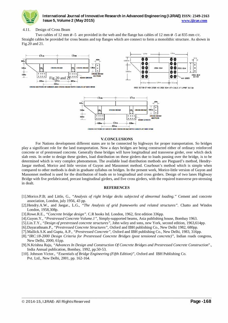
4.11. Design of Cross Beam Two cables of 12 mm ø -5 are provided in the web and the flange has cables of 12 mm ø -5 at 835 mm c/c.

Straight cables be provided for cross beams and top flanges which are connect to form a monolithic structure. As shown in Fig.20 and 21.

Fig.20 and 21

V.CONCLUSIONS For Nations development different states are to be connected by highways for proper transportation. So bridges

play a significant role for the land transportation. Now a days bridges are being constructed either of ordinary reinforced concrete or of prestressed concrete. Generally these bridges will have longitudinal and transverse girder, over which deck slab rests. In order to design these girders, load distribution on these girders due to loads passing over the bridge, is to be determined which is very complex phenomenon. The available load distribution methods are Pieguard’s method, Hendry-Jaegar method, Morice and little version of Guyon and Massonnet method. Courboun’s method which is simple when compared to other methods is dealt in graduate syllabus on bridges. In the present work, Morice-little version of Guyon and Massonnet method is used for the distribution of loads on to longitudinal and cross girders. Design of two lanes Highway Bridge with five prefabricated, precast longitudinal girders, and five cross girders, with the required transverse pre-stressing in dealt.

REFERENCES

[1].Morice.P.B; and Little, G., “Analysis of right bridge decks subjected of abnormal loading.” Cement and concrete association, London, july 1956, 43 pp.

[2].Hendry.A.W., and Jaegar., L.G., “The Analysis of grid frameworks and related structures”. Chatto and Windos London, 1958,308p.

[3].Rowe.R.E., “Concrete bridge design”. C.R books ltd. London, 1962, first edition 336pp. [4].Guyon.Y., “Prestressed Concrete Volume.1”, Simply-supported beams, Asia publishing house, Bombay 1963. [5].Lin.T.Y., “Design of prestressed concrete structures”, John wiley and sons, new York, second edition, 1963,614pp. [6].Dayarathnam.P., “Prestressed Concrete Structures”, Oxford and IBH publishing Co., New Delhi 1982, 680pp. [7].Mallick.S.K and Gupta, A.P., “Prestressed Concrete”, Oxford and IBH publishing Co., New Delhi, 1983, 316pp. [8].“IRC:18-2000 Design Criteria for Prestressed Concrete Bridges (post tensioned concrete)”, Indian roads congress,

New Delhi, 2000, 61pp. [9].N.Krishna Raju, “Advances In Design and Construction Of Concrete Bridges and Prestressed Concrete Construction”.,

India Annual publication, Bombay, 1992, pp.50-53. [10]. Johnson Victor., “Essentials of Bridge Engineering (Fifth Edition)”, Oxford and IBH Publishing Co. Pvt. Ltd., New Delhi, 2001, pp. 162-164.

A Study on Design of Prestressed Post-Tensioned Girder by Morice ...

Documents

Transcript of A Study on Design of Prestressed Post-Tensioned Girder by Morice ...