A Study of Thermal Noise

for Enhanced

Laser Interferometer Gravitational-

Wave Observatory

By

Lucienne Merrill

In partial fulfillment for the degree of Physics

Simmons College

May 2008

Advisers: Simmons College: Velda Goldberg Massachusetts Institute of Technology: Gregg Harry

Table of Contents Abstract………………………………………………………………………………….III Acknowledgements…….……………………………………………………………….IV 1 Introduction 3

1.1 Gravitational Waves………………………………………………………...3 1.2 Detection of Gravitational Waves ………………………………………….5 1.3 Thermal Noise…………………………………………………………….11 1.4 Thesis Outline…………………………………………………………….15

2 Background 16

2.1 Mathematical Models…………………………………………………...…16 2.1.1 Brownian Motion…………………………………………………16 2.1.2 Fluctuation-Dissipation…………………………………………....17 2.1.3 Damped Simple Oscillator…………...……………………………18

2.2 Previous Measurements…………………………………………………...20 2.2.1 40-Meter Mark I Prototype………………………………………..20 2.2.2 Experimental Study of Suspensions……………………………….21 2.2.3 Initial LIGO………………………………………………………24 2.2.4 MIT Suspensions Experiment…………………………………….25

3 Materials and Methods 28

3.1 The Experiment…………………………………………………………...28 3.2 The Test Mass…………………………………………………………….29 3.3 The Standoffs……………………………………………………………..35 3.4 The Electronics…………………………………………………………....37

3.4.1 Magnetic Driver…………………………………………………...37 3.4.2 High Voltage Driver………………………………………………38 3.4.3 Vacuum System…………………………………………………...39 3.4.4 Data Recording…………………………………………………....41

3.5 Alignment and Calibration………………………………………………...42 3.5.1 Test Mass Alignment……………………………………………...42 3.5.2 Recoil……………………………………………………………..44 3.5.3 Wire Creaking……………………………………………………..45

4 Experimental Results 52

4.1 BK7 Prisms……………………………………………………………….53 4.1.1 Laser Cut………………………………………………………….53 4.1.2 Un-Cut……………………………………………………………54 4.2 Sapphire Prisms…………………………………………………………...56

4.2.1 Un-cut…………………………………………………………….57 4.2.2 Laser Cut………………………………………………………….58

I

4.2.3 Diamond Dust Wire Cut………………………………………….58 4.3 Tool Steel Clamp………………………………………………………….60 4.4 Initial LIGO Standoffs……………………………………………………61 5 Conclusions 65

5.1 Summary………………………………………………………………….65 5.2 Future Work………………………………………………………………68

A Appendix 69 A.1 Measured Qs……………………………………………………………...69 A.2 Dimensions of Clamp…………………………………………………….75 A.3 Stylus Measurements……………………………………………………...75 Bibliography 77

II

Abstract

The LIGO project (Laser Interferometer for Gravitational Wave Observation) is run by the

California Institute of Technology (Caltech) and the Massachusetts Institute of Technology

(MIT) with the aim of directly detecting gravitational waves for the first time. Thermal noise

within the interferometers limits the sensitivity and must be reduced in the frequency band

where astrophysical sources should produce gravitational waves. Our research investigates a

critical source of such thermal noise in the suspension subsystem of the LIGO

interferometer. The suspension subsystem consists of suspended silica test masses which

have the ability to move freely in response to a gravitational wave. The goal is to have a

suspension subsystem with low mechanical loss and thus high, consistent, Q resonances, so

that, by the Fluctuation-Dissipation Theorem, the thermal noise will be low. In particular,

my work has focused on the thermal noise in the wires produced at the point the wire leaves

the mirror, which in the LIGO detectors, is governed by a standoff. We have analyzed and

tried to improve the Qs of the wire using different standoffs and a variety of techniques to

situate the standoff on the test mass. The results from this research could potentially be very

important for Enhanced LIGO, or even Advanced LIGO, which are the next generations of

this federally funded project.

III

Acknowledgements It is hard to express my gratitude for the many people who have had an impact on my life, in

and outside of school. However, this will be my attempt…

Thank you, especially, to Gregg Harry. You introduced me to LIGO two years ago, and it

has been my obsession ever since. I can not thank you enough for giving me the opportunity

to join the group at MIT for my research this past year, it has been the greatest experience I

could have asked for. I am incredibly lucky to have met you, and I wish the very best for

you, your wife and your lovely daughter.

To Rai Weiss, thank you for spending time with me on the suspensions experiment. I have

really learned a lot from you, and am truly inspired by the dedication you have to LIGO. I

have really enjoyed all of your stories, all of your rants and all of your help. Thank you.

To Velda Goldberg, thank you for being the greatest adviser these past four years. It was in

your Introductory Physics class that I decided to be Physics major… this was the best

decision of my life. Thank you so much.

To Nicolás Smith and Matt Evans, thank you for taking time to help me with the

suspensions project. It was so nice having another person around while taking wire Q

measurements, and pumping down. I have learned a lot from both of you, and wish you the

very best of luck in the future.

To Bob Laliberte, Myron MacInnis and Rich Mittleman, thank you for lowering and raising

the bell jar with me these past months. I am incredibly indebted to your crane lifting

services. I would not have gotten nearly enough done if you hadn’t taken time out of your

work to help me. Thank you.

To Mom, Dad, Brecht and Zora, thank you for supporting me these past four years in my

endeavors around the world.

IV

To all of the girls, there are too many of you to name… thank you for pulling my head out

of the books and showing me what it means to have friends. I have had the greatest

experience these past four years, and will never forget any of you. Good luck and keep in

touch, I will miss you all.

V

List of Figures 1-1 An illustration of the two polarizations of a gravitational wave……………………..5 1-2 The Michelson-Morley fixed mirror interferometer………………………………....6 1-3 A schematic design of the LIGO interferometer…………………………………....8 1-4 The expected total noise in each of LIGO’s 4-km interferometers………………...10 1-5 A graph of the amplitude of a resonating structure at its resonant frequency……...13 2-1 Gillespie and Raab experimental apparatus to test for mechanical loss and thermal

noise in LIGO suspensions……………………………………………………….22 2-2 Measured Q due to standoffs as a function of wire length. Each cross represents the

measurement of the Q of a different wire. Gillespie and Raab, 1994………………23 2-3 Time and frequency domain loss angle measurements at LIGO sites……………...25 2-4 The measured Q and resulting inconsistencies within data for clamps…………….26 3-1 Initial LIGO standoff; a silica cylinder. The standoffs help to define the point at

which the wire leaves the test mass; an attempt to improve the thermal noise in the suspensions……………………………………………………………………….29

3-2 The silica test mass, for experimentation at the LIGO MIT site…………………..30 3-3 The VIRGO clamps used to clamp the steel wire looping around the test mass to the

support structure………………………………………………………………….31 3-4 Support structure sitting on optics table at MIT lab……………………………….32 3-5 Shadow sensors; comprised of an LED and split photodiode……………………..33 3-6 A sapphire equilateral prism, used for experimental tests at the LIGO MIT site…..35 3-7 Magnification of a groove cut into a BK7 prism………....………………………...36 3-8 The bell jar - open and not under vacuum………………………………………....38 3-9 The vacuum system for the suspensions experiment at LIGO MIT……………….40 3-10 The LIGO pendulum suspension and associated degrees of freedom……………..42 3-11 A picture of the wire placed in the standoff, midway along the width of the

pendulum................................................................................................................................44 3-12 Motion of wire above and potentially below standoff in suspension apparatus

……………………………………………………………………………………46 3-13 Wire motion and up-conversion below the BK7 prism standoff with no aluminum

prism ……………………………………….…………………………………….48 3-14 Observed motion of wire with Sapphire prism and aluminum prism set-up

………………………………………………………………...………………….49 3-15 Motion of wire beneath Aluminum prism…………………………………………50 3-16 Motion of the clamp during wire excitation……………………………………….51 4-1 The dimensions for the triangular face of a BK7 right angle prism………………..53 4-2 A side view of a prism standoff above the aluminum position constraint………….55 4-3 The affect of the position constraint on the BK7 Q measurements……………….56 4-4 Dimensions of equilateral Sapphire prisms………………………………………..57

1

4-5 Complete distribution of Q measurements for all of the sapphire prisms tested…...59 4-6 The size and layout of the tool steel clamp………………………………………..60 4-7 The clamp situated and glued onto the test mass, in place of a normal standoff…..61 4-8 Energy decay for RFB excitation with silica rod standoff…………………………62 4-9 Energy decay for RLR excitation with silica rod standoff…………………………63 4-10 Initial LIGO Silica Rod results with and without Aluminum prism……………….64 5-1 Abrasion of Silica and BK7 from contact with wire……………………………….66 5-2 Abrasion of Sapphire from contact with wire……………………………………...66 5-3 Total distribution of Q’s for the different standoffs used on the experimental

suspension at MIT………………………………………………………………...67

List of Tables 2-1 Frequencies and Q measurements for the left arm end and vertex masses in the 40-

Meter Mark I Prototype ………………………………………………..…………21 2-2 Frequencies and Q measurements for the right arm end and vertex masses in the 40-

Meter Mark I Prototype …………………………………………………………..21 2-3 Q measurements at resonant frequencies taken from Scientific Run 2 at the Hanford

interferometer……………………………………………………………………..24 3-1 Sensitivities for each shadow sensors measured in mV/mil……………………….34 3-2 Recoil energy ratios between the wire and support structure………………………45

2

Chapter 1 Introduction The research undertaken for the completion of this thesis was conducted as a part of the

Laser Interferometer Gravitational-Wave Observatory (LIGO) project at Massachusetts

Institute for Technology (MIT) in Cambridge, Massachusetts. LIGO is at the forefront of

physics research, where the main goal is to detect gravitational waves and strengthen our

knowledge of astrophysical processes.

1.1 Gravitational Waves The quest for gravitational waves begins with a thirst for more knowledge about the depths

of the universe. In the four-dimensional world that Albert Einstein imagined in his General

Theory of Relativity, these waves exist as faint ripples traveling across the universe at the

speed of light. These space-time disturbances can be thought of as analogous to

electromagnetic waves, where the ripple from a source of space-time curvature propagates in

a gravitational field [16].

In Einstein’s General Theory of Relativity, occurrences, which are described by classical

mechanics as taking place due to the force of gravity (i.e. free fall), are described by inertial

motion within a curved geometry of space-time. The curvature of space-time has been

described several ways. The most commonly used depiction elicits the idea of a heavy

spherical object sitting on a sheet of rubber, thick enough that it doesn’t break under the

weight of the object, and thin enough that there is a perturbation in the sheet due to the

weight of the sphere. In an attempt to describe this relationship, Einstein developed a set of

field equations, logically known as the “Einstein field equations” [13]. These equations relate

space-time content and space-time curvature (think about the heavy sphere on the rubber

sheet) as follows:

abab TG !" (1.1)

3

Gab is the Einstein tensor; Tab is the energy-momentum tensor and k is a constant. The stress

energy tensor, which is the source of the gravitational field, includes stress, the density of

momentum, and the density of energy including the energy of mass [13]. The constant ! in

this equation can be thought of as similar to the constant k in Hooke’s law, Fs = -ksx, which

is the measure of the stiffness of a particular spring being either stretched or compressed a

distance x, because the constant in the Einstein Field Equation is a measure of the stiffness

of space. The derived value for this constant was determined to be 4

8cG# , where G is the

gravitational constant and c the speed of light, the 4

1c

indicates just how taut space-time

really is.

According to Einstein’s Field Equation, it would require a heavy body to change the

curvature of space-time, as it is very stiff, and if a heavy body moved around in a certain way

it would produce ripples or gravitational waves in the fabric of space-time, much like ripples

in a pond.

Gravitational waves are formed by non-spherical motions of mass in space-time and

propagate by stretching space in one transverse direction and compressing it, at the same

time, in the other transverse direction [16]. This is compared to electromagnetic waves,

which is the motion of charge in one transverse direction. As gravitational waves pass

through any galaxy, they expand and contract in a manner as shown in Figure 1-1, in cross

and plus polarizations. These contractions are sometimes referred to as “cross” and “plus”

polarizations in essence of their motion. The deformations shown in Figure 1-1 are

essentially tidal effects, but time-dependent rather than static.

4

Figure 1-1. An illustration of the two polarizations of a gravitational wave. The arrows indicate in which

way it will expand or contract [28].

As a result of a typical passing gravitational wave from an astronomical event, objects will

change in length by 1 part in 1021, which is an extremely small effect, for even the strongest

astrophysical sources present in the universe. In order to see these small ripples, gravitational

wave detectors need to be sensitive enough to see a change in length, "$L 10-18m [12] in a

4-km long system.

1.2 Detection of Gravitational Waves LIGO is part of a world-wide collaboration in the detection of gravitational waves. After a

few initial detectors were created (for more information look up Joseph Weber and

Aluminum bars), it was decided that LIGO would try and use an interferometer, based on

the concept developed by Albert A. Michelson and Morley in the 19th century.

In 1887 Michelson and Morley aspired to measure the speed of the earth relative to the

luminiferous aether (the only medium through which scientists used to believe light could

propagate). Michelson and Morley, assuming the Galilean rules of relativity hold, thought

that the relative speed of light would be slower in the direction of motion of the earth.

5

Therefore, they decided to build an apparatus, known as an interferometer which could

detect the speed of the aether wind. Here is a diagram showing Michelson's apparatus:

Figure 1-2. The Michelson-Morley fixed mirror interferometer [29].

The Michelson-Morley interferometer depends upon a light from a spectral line source (even

though that says coherent light source above) entering a beam splitter (semi-silvered mirror),

traversing two perpendicular arms and reflecting off one suspended mirror and another fixed

mirror. The detector was orientated so that one arm had a constant pattern seen on the

detector (the fixed mirror), while the other arm could be moved by the motion of the earth

and then cause a different interference pattern on the detector [17]. What Michelson and

Morley were looking for were changes in the fringe pattern on the detector, which are the

alternating bands of light and dark which depend upon the interference pattern. When light

is constructively interfering, the detector will see bright fringes, when the light is

destructively interfering (or canceling each other out), the fringe will be much darker. What

makes the interferometer such a precise measuring instrument is that these fringes are only

one light-wavelength apart. In visible light, about 590 nanometers --that corresponds to

6

1/43,000th of an inch! Any movement along the optical axis by either flat mirror will cause

the fringes to shift an equal amount [17].

What Michelson and Morley actually discovered was that the speed of light does not change

with motion in any direction. The results of this experiment also proved that Galilean

relativity was not correct. However disappointed Michelson and Morley may have been with

the results of their experiment, the results and design of their interferometer became a

stepping stone for special relativity and is now being used as a means for detecting

gravitational waves.

A crucial difference between an interferometric gravitational wave detector and the

Michelson-Morley apparatus is that one of the Michelson-Morley mirrors is rigidly mounted

to the same table as the beam-splitter. The only change in path-length could be felt from

one direction, in their case, they wanted the direction of motion of the earth. In the Laser

Interferometer Gravitational-Wave Observatory, you want all the optics to be as free to

move as possible due to the manner of propagation of the gravitational waves, thus the

suspensions. It is precisely the relative motion between beam-splitter and mirror that you are

hoping to see.

Very precise length measurements can be made with an interferometer because the

wavelength of a monochromatic light source is a factor in how sensitive measurements can

be. This is one reason why interferometry can be used to measure the change in length of a

gravitational wave. For instance, if "=400nm, this gives a precision of 100 nm or 10-4 mm for

an interferometer [17]. Which is, of course, a long way from the precision you need to see a

gravitational wave. You don’t need for the relative position of the mirrors to change by a

quarter wave length to detect a signal. Much smaller changes will result in changes in

brightness at the photodiode, which can be detected.

The interferometers developed by LIGO also depend on the light from a laser entering a

beam splitter, traversing two orthogonal arms (all in vacuum), and reflecting off suspended

mirrors at the end of the arms (see Figure 1-3). As a gravitational wave passes the position of

the suspended mirrors would change by a small amount, thus changing the length of at least

7

one of the arms, and changing the phase of the laser as it travels back along its path. Figure

1-1 in Section 1-1 is a good explanation as to why at least one of the arms will change as the

result of a passing gravitational wave. As a gravitational wave passes by, objects change in

length by one part in 1021, which for the distance from the sun to the earth is about one

atomic diameter. This is an extremely small effect, and it is for this reason that the laser used

in the interferometer design must have a very small wavelength, so that the slightest change

in phase will be noticed in the return signal. The weak effect generated by the gravitational

wave indicates that the equipment used to detect them need to be as sensitive as possible to

detect this one part in 1021 change in the mirrors position, hence the laser’s short

wavelength. Also, it should be noted that despite the importance of a shorter wavelength,

but it is also important to have a laser that you can reduce the noise down to the level limited

by quantum mechanics, hence the reason why LIGO uses a 1064 nm Nd: YAG

(Neodymium-doped Yttrium Aluminum Garnet) laser. The difference in fringes on the

detector with just a 1064 nm laser will be sensitive to motion of about 1/940,000 of a meter.

Figure 1-3. A schematic design of the LIGO interferometer [28].

However, there is a limit to what wavelength laser LIGO can use in its interferometers. As a

gravitational wave passes, not only does it change the length of time for the laser’s signal in

one arm, but it also increases the wavelength of the light by a factor of ( 0211 h% ), where h0 is

the amplitude of the wave. This means that light waves are actually stretched by the passing

8

of a gravitational wave, the distances between waves crests increases at the same time as the

distance between the mirrors grow. In order to make the effect of a gravitational wave

visible, the LIGO group chose extreme values for the ratio of light wavelength to arm

length, and for h0 [14]. The physical arm length for both of the LIGO detectors is 4 km;

however, they have employed the use of Fabry-Perot cavities to effectively increase the arm

length. Fabry-Perot cavities are used to reflect the laser light between two mirrors a total of

75 times before re-emitting the light back towards the beam splitter, effectively changing the

length of the interferometers arms [19].

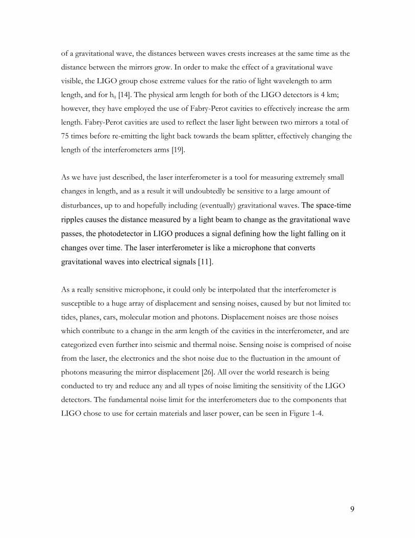
As we have just described, the laser interferometer is a tool for measuring extremely small

changes in length, and as a result it will undoubtedly be sensitive to a large amount of

disturbances, up to and hopefully including (eventually) gravitational waves. The space-time

ripples causes the distance measured by a light beam to change as the gravitational wave

passes, the photodetector in LIGO produces a signal defining how the light falling on it

changes over time. The laser interferometer is like a microphone that converts

gravitational waves into electrical signals [11].

As a really sensitive microphone, it could only be interpolated that the interferometer is

susceptible to a huge array of displacement and sensing noises, caused by but not limited to:

tides, planes, cars, molecular motion and photons. Displacement noises are those noises

which contribute to a change in the arm length of the cavities in the interferometer, and are

categorized even further into seismic and thermal noise. Sensing noise is comprised of noise

from the laser, the electronics and the shot noise due to the fluctuation in the amount of

photons measuring the mirror displacement [26]. All over the world research is being

conducted to try and reduce any and all types of noise limiting the sensitivity of the LIGO

detectors. The fundamental noise limit for the interferometers due to the components that

LIGO chose to use for certain materials and laser power, can be seen in Figure 1-4.

9

Figure 1-4. The expected total noise in each of LIGO’s 4-km interferometers (green dotted curve), showing the various contributions to the first interferometer’s noise [27].

In the figure above the predicted limiting region for the LIGO interferometers is shown by

the green dotted curve titled “total noise”. The ability to hear gravitational waves is limited

by the detectors vulnerability to all of the plotted noise sources, as they limit different

frequency domains in which gravitational waves might propagate by all of the noise they

produce. LIGO is designed to be able to sense gravitational waves formed by certain

astrophysical events in the 40-7000Hz frequency range [26], however, because LIGO has not

detected a gravitational wave yet, it only means that the instrument is still too limited by the

noise. As shown in the strain sensitivities above, LIGO is limited in the lower frequencies by

seismic noise, in the middle frequencies by suspension thermal noise and in the higher

frequencies by shot noise from the laser.

10

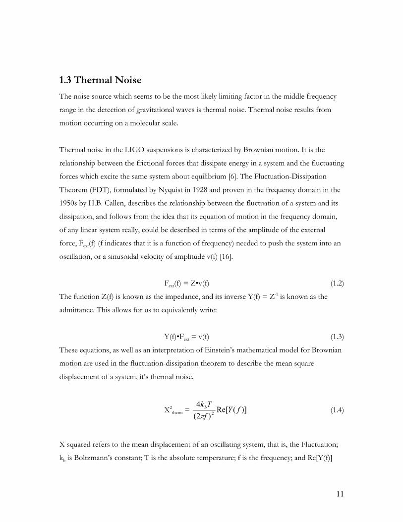
1.3 Thermal Noise The noise source which seems to be the most likely limiting factor in the middle frequency

range in the detection of gravitational waves is thermal noise. Thermal noise results from

motion occurring on a molecular scale.

Thermal noise in the LIGO suspensions is characterized by Brownian motion. It is the

relationship between the frictional forces that dissipate energy in a system and the fluctuating

forces which excite the same system about equilibrium [6]. The Fluctuation-Dissipation

Theorem (FDT), formulated by Nyquist in 1928 and proven in the frequency domain in the

1950s by H.B. Callen, describes the relationship between the fluctuation of a system and its

dissipation, and follows from the idea that its equation of motion in the frequency domain,

of any linear system really, could be described in terms of the amplitude of the external

force, Fext(f) (f indicates that it is a function of frequency) needed to push the system into an

oscillation, or a sinusoidal velocity of amplitude v(f) [16].

Fext(f) = Z•v(f) (1.2)

The function Z(f) is known as the impedance, and its inverse Y(f) = Z-1 is known as the

admittance. This allows for us to equivalently write:

Y(f)•Fext = v(f) (1.3)

These equations, as well as an interpretation of Einstein’s mathematical model for Brownian

motion are used in the fluctuation-dissipation theorem to describe the mean square

displacement of a system, it’s thermal noise.

X2therm = )](Re[

)2(4

2 fYfTkb

# (1.4)

X squared refers to the mean displacement of an oscillating system, that is, the Fluctuation;

kb is Boltzmann’s constant; T is the absolute temperature; f is the frequency; and Re[Y(f)]

11

refers to the real part of the admittance, the Dissipation. This equation is the Fluctuation-

Dissipation Theorem.

The suspension’s thermal noise is described by displacement noise, as shown in equation 1.4,

which is characterized by certain amplitudes of motion of the wire holding the mirror in the

interferometer. Brownian motion relates the fluctuation, or random walk, of the degrees of

freedom of the system and its mechanism for dissipation.

The quality factor, the Q, of a system is the dimensionless measure of the ratio between the

elastic restoring forces to the dissipative forces. The formal definition of Q:

)(2

cycleoneinEEQ

lost

stored

&&$&

"#

(1.5)

lost

stored

PeriodE&

"'

The second equation is found by multiplying numerator and denominator by '' to get the

period. The Q is then described in the frequency domain by:

)2/1((max)Powerf

fQ$

" (1.6)

Where f is frequency and #f is the full width of the resonance peak in the frequency response

of the system, measured at the level of half of the maximum power [16].

The Q is used to compare the time constant for the decay of an oscillating system is

amplitude with its oscillation period [15]. Q is the quality factor of a resonance related to the

decay time. It can be found from the ratio, which is the mechanical loss, as defined above.

An oscillating system with a Q<1 is said to be critically damped which really means that the

system isn’t oscillating at all, see Figure 1-5 for a range of values for Q [17].

12

Figure 1-5. A graph of the amplitude of a resonating structure at its resonant frequency. If only a very little damping occurs in the system then the Q value is very large and the amplitude of oscillation at resonance is illustrated by a sharply defined peak. If the damping is larger, then the Q value is much smaller so that the amplitude of oscillation at resonance is much lower and described by more of a flattened curve. [18]

The test masses used in LIGO are large cylindrical silica mirrors suspended by a single loop

of steel piano wire; this makes them pendulums. These pendulums are characterized by their

many modes of vibration, two of the most relevant modes and part of the motivation to the

research involved in this paper, are the “violin modes” of the pendulum wires and the

vibration modes of the test mass itself. The “violin modes” of the pendulum wires, appear as

a nearly harmonic sequence with fundamental frequency:

lnmmgf

'21

1 " (1.7)

Where f1 is the first harmonic of the system; m is the mass of the pendulum; g is the

gravitational constant; n is the number of wires supporting the mass and mw is the mass of an

individual wire. These modes will appear with Q’s of the same order as that of the pendulum

mode, and for the same reason. Thermal noise displacement of the test mass itself is

suppressed by the large mass ratiowmm ; only at the high Q resonant peaks are these modes

likely to contribute visibly, in the presence of the other noise sources [16].

13

The Q’s in real physical situations vary greatly, and therefore there are a variety of ways to

measure the Q of an oscillating system. The Q in the suspension systems for LIGO can be

measured by the width in resonance, because Q= $0/#$, as well as by the ring-down time of

oscillation in the wire, Q = %f&, where f is the resonant frequency and & is the exponential

decay time constant of the oscillation. The internal dissipation of energy in the wires of the

suspension set up in LIGO determines the Q of the wire, and thus the thermal noise for the

suspension system, as Q is inversely related to the loss angle ( at the resonant frequency $0,

by:

Q=)(

1

0'( (1.8)

Therefore, by equation 1.5, the smaller the amount of dissipation is in a system, the higher

the Q will be. In LIGO it is desirable to concentrate the energy in a very narrow frequency

band around the resonant frequency, as one can see from Figure 1-5, to have a large quality

factor [10]. In order to minimize the effects of this thermal energy on the LIGO noise

spectrum (Figure 1-4), it is necessary to create a suspension system whose energy is

concentrated in its own narrow resonant frequency band, so that it can be easily filtered

from the gravity wave spectrum with little loss of observing bandwidth. A higher Q also

means that the measured loss in the system is low and there will be less strain on the

interferometer in the thermal noise region of the measured frequency range.

Currently at the LIGO sites the Q’s measured on the suspension wires vary from 30,000 to

160,000 on any given day (see Chapter 2 for more information). Such a huge variation in Qs

also creates a huge variation in the thermal noise exhibited by the suspensions for LIGO.

This variation is what gives backbone to some of the research currently being conducted at

the LIGO MIT lab, where the ultimate goal is to understand the fluctuation in Q’s by

understanding what is causing the dissipation.

There are really only a few things which can be physically changed in the LIGO suspensions

which may play a part in the loss of energy. One of these in particular is the standoff which

defines the boundary conditions of the wire on the test mass. A recent idea which was

proposed regarding the LIGO suspensions suggested that the point at which the wire leaves

the test mass is rubbing, causing friction and noise. This noise will, in effect, limit the

14

sensitivity of the next generation of interferometers, as it will prevent LIGO from being able

to distinguish between a change in displacement from a gravitational wave or from the

displacement caused within its own suspensions.

1.4 Thesis Outline The aim of our research presented in this paper is to develop a method to reduce excess loss

and minimize slope coupling in the LIGO suspensions by redefining the boundaries

between the wire and the test mass, therein producing higher, more constant Q’s in the

suspensions and ultimately minimizing thermal noise.

This thesis presents the theoretical model developed to describe the power spectrum of

Brownian motion of the LIGO suspensions, as well as an experiment developed to predict

the Brownian motion in the LIGO suspensions for the next generation of interferometers,

focusing on, in particular, the friction between the pendulum and the wires suspending it.

The thesis plan is as follows: in Chapter 2, we will develop the mathematical model used to

describe the system we are looking at, as well as look at past research regarding the

dissipation in the prototype and initial LIGO detector suspensions. In Chapter 3, we

describe the experimental set-up. In Chapter 4, we analyze and compare the results provided

from the experiment with past measurements. In Chapter 5, we present our conclusions,

discussion and potential future work for minimizing the suspension thermal noise in the next

generation of LIGO interferometers. In the Appendix, we include the full index of

measurements taken at LIGO MIT.

15

Chapter 2

Background In this chapter we will provide previous models and measurements taken in the frequency

domain to analyze and improve the Q for the different generations of the interferometers.

Initially, we will look at the mathematical models which are used to describe the thermal

noise in the LIGO suspensions and use the simple model of a damped harmonic oscillator

to show how to make use of these models, and then we will look at the experimental models

which were used to predict suspension thermal noise for the different generations of LIGO

interferometers.

2.1 Modeling Thermal Noise In this section we will present the mathematical models which are used to describe thermal

noise in the LIGO suspensions along with a simple example to demonstrate its use.

2.1.1 Brownian Motion Brownian motion is the random fluctuations of particles in a liquid or gas. It was discovered

in the 1800s by Robert Brown (for whom it is named), who observed the random motion of

small grains of dust and pollen suspended in water [16]. The mathematical model developed

to describe Brownian motion has been applied to random fluctuations for particles as well as

things such as stock market fluctuations and the evolution of physical characteristics of

fossils [28].

The mathematical model to describe the random motion of a damped harmonic oscillator

with mass m, a stiffness in the spring k, subject to a frictional force of the form

(where f is the coefficient of velocity), is described using the stochastical

differential equation [24].

fvFfriction )"

thFkxxfxm "%% !!! (2.1)

16

Fth is the random force exhibited on the particle, described with a white spectral density of:

. This equation of motion is easier to solve by converting it into the

frequency domain by replacing , this is known as a Fourier Transform [5].

Finding the power spectral density of the position of the mass requires multiplying the

continuous Fourier Transform and its complex conjugate together. This process yields the

following result:

TfkF Bth 4)(2 "'

tiextx '')()( "

22222

)(4)(

'''

fmkTfkx B

%)" (2.2)

This model has an eigenfrequency at mk

"20' , and a graph of this function with all the

parameters set except the varying position spectrum and the frequency would show a peak at

this frequency. If the frictional coefficient of velocity is small, then the response of the

particle is extremely sharp at $0, and the sharpness of this peak can be described by the Q.

As was mentioned in Chapter 1, the Q is defined as Q= $0/$, and a high Q means a small

loss angle, and as a result an improved thermal noise limit for the LIGO interferometers [4].

2.1.2 Fluctuation-Dissipation Theorem Another useful description, which produces the same results as the Brownian motion

derivation above, is the Fluctuation-Dissipation Theorem (FDT). This description within the

frequency domain was derived by H. B. Callen and others to describe the dissipation in any

system caused by the same thing which causes the system to fluctuate, or move to disorder

[16]. The spectral density of the random force as given by the FDT is given by:

]Re[4)(2 ZTkF Bth "' (2.3)

Re[Z] is the real part of the impedance; T is the absolute temperature and kB is Boltzmann’s

constant. The position spectral density could also be described in a similar manner, except

using the admittance:

]Re[4)( 22 YTkx B &"

'' (2.4)

The real part of Y (the impedance) is given by Fext(f) = Z•v(f), Y(f)•Fext = v(f) and Y(f) = Z-1.

For a simple oscillator the impedance is given by:

17

2222

32

)()(fmk

mkifY'''''

%))%

" (2.5)

Solving for the real part of the admittance (the inverse of the equation above) and

substituting it into equation 2.4 we find the same result we did with the Brownian motion:

22222

)(4)(

'''

fmkTkx B

%)"

This shows that the use of Brownian Motion and the Fluctuation-Dissipation Theorem is

interchangeable when describing a simple oscillator [24].

2.1.3 Damped Simple Oscillator A general model to describe damping in a harmonic oscillator is a form of Hooke’s law F =-

kx, where the spring constant is taken to be complex [8]:

xikF )](1[ '*%)" (2.6)

Using Newton’s second law and the equation for admittance, we can begin to solve for the

general form for the spectral density of displacement due to thermal noise for a simple

harmonic oscillator:

Making sure to apply the complex spring constant as a part of the equation for force we find

the admittance to be:

2222

2

2

2

2

22

)()()(

)()()()(

)()(1

)1(1

('('''

('('

(''

'('

'('

kMkkMki

ikMkikMk

ikMki

Mkiki

MikiY

%)%)

"

"))))

+%)

")%

")%

"

As was mentioned before, the fluctuation-dissipation theorem describes the displacement

spectral density due to thermal noise by using the real part of the admittance, this requires

adjusting the equation above into the complex number form (a + bi), where a is the real part

and b is the imaginary, and taking the real part a, as the admittance. This results in the

admittance being of the following form:

18

2222 )(]Re[

('('

kMkkY

))" (2.7)

The spectral density due to thermal noise can thus be derived by applying the fluctuation-

dissipation theorem to the real part of the admittance as follows:

])[(4]Re[4

22222222

('('

'# kMkkTkY

fTkx BB

therm ))+"" (2.8)

In the LIGO detectors, the maximum sensitivity is around 100 Hz, and around those

frequencies the thermal noise can be described by:

5

202 4

~)('

(''

MTkx B (2.9)

This equation is a result of assuming that $0 ‹‹ $, where $0 is measured to be around 1Hz

andMK

"20' (the natural frequency of a pendulum) [6]. This damped oscillator has a Q of

this sort given by:

)(1

0'("Q (2.10)

The angle )('( is described as the angle at which the spring will lag the force in a linear

response to a force. The frequency 0' describes the loss angle at the resonant frequency of

the suspension [24]. As the reader may recall from the previous chapter, the Q for the

“violin modes” appear in the same order as the Q’s for the pendulum mode, and for the

same reason. Therefore, the dissipation in the oscillation of the wires occurs for the same

reason as the dissipation in the oscillation of the pendulum.

Peter Saulson remarks in his book, “Fundamentals of Interferometric Gravitational Wave

Detectors”:

“The Q of such modes should be able to reach the inverse of the loss angle ( of the

mirror substrate. There is, unfortunately, no “improvement factor” comparable to

that applying to the pendulum mode and the violin modes. This is a crucial

distinction. The only way to achieve sufficiently high Q is to find the right mirror

material” [16].

19

The right mirror material, that is the material used for the LIGO test masses, is silica, which

has excellent optical properties and a loss angle . Despite this small loss with the

mirror material, there is still an apparent loss in the suspensions system associated with the

wire-mirror relationship, and this loss can be observed by inconstant, low Q’s as a result of

some early work prior to and during the Initial LIGO scientific runs.

610),(

2.2 Previous Measurements In this section we will look at the work done by others to describe and model the thermal

noise and Q’s in the suspension from the 40-Meter Mark I Prototype, Initial LIGO and

some experimental apparatus’ created to test the loss in future LIGO suspensions.

2.2.1 40-Meter Mark I Prototype In 1992, A. Gillespie and F. Raab investigated the violin resonances in the Test Mass

Suspensions of the 40-Meter Mark I Prototype [10], which was the prototype for the actual

LIGO interferometers which are operating today. As it has been mentioned before, the

focus of the research in this paper investigates the wire part of the suspensions in the LIGO

interferometer, and in particular the dissipation of energy as a result of the boundary

conditions between the wire and the test mass. The reason for dissipation of energy and thus

the systems fluctuations can be measured by the Quality factor and this was done to test the

suspensions prior to building LIGO, to help characterize the materials which were going

into the interferometer.

Gillespie and Raab created an experiment employing a similar method to resolve Q values as

the research in this paper did; driving the wires of the test mass at resonance, turning off the

drive, and measuring the ring-down times by filtering the interferometer output,

heterodyning it against a local oscillator with a 1 Hz offset and using the decay of the beat

note [10]. There are two different types of test masses in the 40-Meter Mark I Prototype, end

and vertex masses. The difference between the two test masses is that the vertex masses

have no magnets (which were used to drive the end masses on resonance), different

20

thickness of wires and different control blocks. The resulting Qs for the end mass and vertex

mass for the right and left arms can be found in the tables below:

LEFT ARM END MASS LEFT VERTEX MASS Frequency (Hz) Q Frequency (Hz) Q

319.65 13,000 594.35 242,000 324.9 13,000 596.675 335,000

326.075 19,000 598.15 43,000 328.45 16,000 605.025 112,000

Table 2-1. Frequencies and Q measurements for the left arm end and vertex masses in the 40-Meter Mark I Prototype [10].

RIGHT ARM END MASS RIGHT VERTEX MASS Frequency

(Hz) Q Frequency (Hz) Q

505.85 66,000 592.7 295,000 506.875 118,000 592.8 295,000 512.85 23,000 596.425 356,000 514.9 16,000 600.225 163,000

Table 2-2. Frequencies and Q measurements for the right arm end and vertex masses in the 40-Meter Mark I Prototype [10].

Gillespie and Raab point out in their paper that the difference in frequencies may be

explained by differences in the suspensions, such as the fact that the diameter varied

between the different test masses. They indicated that there was at most about a 50-'m

difference between wire diameters for each test mass. Despite the difference in diameters

between different test masses, there still appears to be quite a variation of Q’s from

individual test masses themselves.

These variations in Q values found by Gillespie and Raab in the prototype interferometer

only begin to illustrate the initial problem with an unknown dissipation in the LIGO

suspensions.

2.2.2 Experimental Study of Suspensions

21

After the tests in the 40-Meter Mark I Prototype, Gillespie and Raab published a paper

entitled “Suspension Losses in the Pendula of Laser Interferometer Gravitational-Wave

Detectors” [2]. This paper highlighted an experiment they did to test the mechanical loss and

thermal noise of the test mass suspensions of the LIGO detector.

The model suspension system that they used consisted of a 1.6kg cylinder of fused silica,

suspended by two loops of 75-'m diameter steel music wire (Figure 2-1).

Figure 2-1. Gillespie and Raab experimental apparatus to test for mechanical loss and thermal noise in LIGO suspensions [2]. The losses in the suspensions were obtained from the Q’s of the resonances, exciting the

wire into resonance and measuring the decay time of the oscillation. Gillespie and Raab

proposed that the mechanical loss in the suspensions were a result of either how the wire

was clamped the support structure, how it was clamped to the test mass, or both. Initially,

they thought to measure the variation in Q’s as a result of exchanging how the wire was

clamped to the support structure, thereby varying the type of clamp holding the test mass to

the suspension. The results concluded that “no difference in the Q’s was found between the

two clamping methods” [2].

22

The next area where Gillespie and Raab thought there may be mechanical loss was at the

clamping point between the wire and the test mass, namely, the standoff. They tested fused

silica prisms (13 mm x 2 mm equilateral triangles) and fused silica rods (13 mm x 2 mm in

diameter). Of the two standoffs that they tested, they used three different methods to hold

the standoff against the test mass: pressure from the wire with no glue, glued onto the test

mass with cyanoacrylate based glue, or attached to the test mass with a vacuum sealant

epoxy. The data that Gillespie and Raab found for the violin mode losses was divided into

two frequency ranges, and the range which produced the interesting results falls between 1

Hz and 2 kHz. They use a simple scaling relation between the Q of the violin resonances and

the length, l, of the wire to model frequency independent losses at the endpoints:

)(1),( '('(l

l " (2.11)

Their results can be seen in Figure 2-1, a plotted graph of this relationship, and what was

noted in their paper was the following: “the spread in the points at a single length indicates

the variation in the Q’s from wire to wire. The data support the hypothesis that the losses

occur at the endpoints” [2].

Figure 2-2. Measured Q due to standoffs as a function of wire length. Each cross represents the measurement of the Q of a different wire. Gillespie and Raab, 1994, [2].

23

The variation in Q’s as a result of analyzing the endpoints where the wire and test mass

meet, within the same wire length, just gives more evidence to the fact that the loss from the

endpoints have been a potential problem and still are a potential problem in the LIGO

detectors.

2.2.3 Initial LIGO After the second scientific run of Initial LIGO was built and running, S. Klimenko, F. Raab,

M. Diaz and N. Zotov conducted tests on the LIGO suspensions to investigate violin modes

at the LIGO sites. The tests involved integrating the noise for 1 minute, using a program

called LineMonitor and analyzing the first two harmonics for each violin mode [29]. What

they discovered can be seen in the following table:

Frequency (Hz) Q

343.745 39,000 343.814 143,000 344.051 70,000 344.11 143,000 349.201 116,000 349.245 90,000 349.282 90,000 349.659 175,000

Table 2-3. Q measurements at resonant frequencies taken from Scientific Run 2 at the Hanford interferometer [29]. The Q’s from the violin modes in the suspensions are represented in Table 2-1 above, and

show an inconsistency in Q’s within a very small frequency band. This says that despite the

knowledge of excess dissipation in the wires at the endpoints on the test mass before the

LIGO detectors were built, nothing was done to correct it, leaving it as a problem for the

next generation of interferometers.

Another, more recent investigation into the violin modes and their contribution to the

thermal noise spectrum, are measurements taken at the LIGO sites separately by Gregg

24

Harry and David Malling. David Malling analyzed his date in the frequency domain, and

Gregg Harry in the time domain, both with results indicating that the test mass wire

suspension violin modes are much lower than anticipated with the material properties of the

suspensions. The following histograms indicate these low Q’s, as well as an inconsistency in

values between measurements.

Figure 2-3. Time and frequency domain loss angle measurements at LIGO sites[32].

These measurements have been sufficient evidence to begin experimenting with the wire

suspensions and the associated losses in different suspension set-ups on a test rig at MIT.

2.2.4 MIT Suspensions Experiment Even more recent investigations into thermal suspension noise were made by Gregg Harry

of Massachusetts Institute of Technology and Steve Penn of Hobart, William and Smith

College, looking into the causes for dissipation in the LIGO suspensions. Initially their

thoughts, like those of Gillespie and Raab in 1994, lead them to the clamps of the

suspension system. In at least one of the talks given to present the findings, it is mentioned

that there is some mysterious change in Q, which is not consistent between optics and they

25

are typically lower than the expected value. At MIT, Gregg Harry and Steve Penn (with the

help of many others) set up a test mass to test different clamps, analyze the decay time of the

oscillation after exciting the wire, and determine the Q (as Gillespie and Raab did).

Gregg and Steve measured the Q’s in the suspensions as a result of three different types of

clamps: the Initial LIGO clamps, the Collet Clamp and a VIRGO inspired clamp. The

measured Q’s are shown in Figure 2-3 below:

Figure 2-4. The measured Q and resulting inconsistencies within data for clamps [created using old data from MIT lab notebook by author].

Figure 2-3 is a good indication that there must be another factor which can improve the

inconsistencies in Q measurements, because the clamps did not appear to make much

improvement upon the variation or value of Q’s, and these results indicate there is still

excess dissipation and thermal noise in the suspensions which may limit LIGO’s sensitivity

to gravitational waves in the nearby future.

In preparation for the next generation of LIGO interferometers, the predicted factors

limiting the sensitivity of the interferometer do need to be investigated, and one of those is

very likely excess loss in the test mass suspensions as a result of poorly defined boundary

conditions between the wire and the test mass. The inconstant Q values observed at the

26

prototype detector, at both sites and at an experimental test rig at MIT is the motivation to

begin experimentation with the standoffs on the test masses for the next generation

interferometer.

27

Chapter 3 Materials and Methods In this chapter we provide a description of the experimental apparatus, the LIGO

suspension and the measuring system. The measurements taken using this apparatus were

performed from September 2007 to April 2008.

3.1 The Experiment In the LIGO interferometers, the most important objects are the test masses, as they are the

part of the interferometer which responds to the vibrational motion of a passing

gravitational wave. In each interferometer, the optic (test mass) is suspended as a pendulum

from vibration isolation platforms to prevent external disturbances from affecting the

sensitivity of their outputs within the gravitational wave band. The test masses which,

geometrically, are huge cylinders comprised of fused silica, weigh around 10.5 kg each. The

test masses are suspended by a steel piano wire passing around the optic in a single loop

equidistant across the test masses sides. Small, grooved glass rods (standoffs) are glued to the

side of the optic a few millimeters above the center of mass to define the suspension point

(the point where the wire leaves the test mass) and minimize frictional losses.

28

Figure 3-1. Initial LIGO standoff; a silica cylinder. The standoffs help to define the point at which the wire leaves the test mass; an attempt to improve the thermal noise in the suspensions.

Thermal noise is managed in the LIGO interferometers by placing resonances above or

below the detection band wherever possible, and by choosing materials and assembly

techniques which yield high resonance Q’s [19]. The purpose of my research conducted at

MIT was to experiment with the standoffs placed on the test masses to minimize frictional

loss, and try to find a particular standoff which would yield a higher, non-varying Q in the

suspension wires. The standoffs consist of a variety of materials, shapes and sizes to help

define the point at which the wire leaves the test mass in its loop around it, see Figure 3-1

for a detailed image.

3.2 The Test Mass The test mass is actually a pendulum which consists of a mass hung by a steel wire from a

support structure.

The mass (Figure 3-2) is made of fused silica, shaped into a cylinder 24 x 10 cm thick. The

steel wire wraps around the middle of the test mass, so that it is equidistant from the sides of

the cylinder.

29

LIGO test mass

Figure 3-2. The silica test mass, for experimentation at the LIGO MIT site. (Photograph taken by Lucienne Merrill)

The steel wire is clamped to the top of the support structure, in a series of three clamps

(Figure 3-3). This clamp set up is actually different than that which is used at the LIGO sites.

(As was mentioned in Chapter 2, before the idea of improving the Q of the wire via the

standoffs arose, there was the idea that the clamp would improve the Q of the wire.

However, after several trials with different clamps and no improvements, the experiment

was left with this new set of clamps and a new experiment under way.) After the wire leaves

the test mass (on both sides), it is fastened initially into a set of clamps, with dimensions 3 x

1.1 x 1 cm and grooves cut through their centers to hold the wire snugly in place. When

hanging the test mass, it is necessary to fit the wire into this grooved clamp first, before

attempting to work it through the other two sets of clamps. Once the wire is sitting in the

groove, it is necessary to screw down the clamp together, to ensure it isn’t going anywhere.

Once the wire ends are secured in the first set of clamps, the two wire leads are positioned

across cylindrical pins (for directional purposes) and into a second set of clamps. The

second set of clamps is an exact replica of the first set, except they don’t have a groove cut

into them for the wire to travel along. Instead, the wire is just pinned down by the clamp

using screws situated in the clamp. The final set of clamps is an interesting pair; they provide

30

a smaller area for the wire to be pinned against, as they are approximately 1.6 x 0.7 x 1 cm,

but are created with a spring in the back of them. There is no known reason why these

clamps were made the way they were, but it is possible they provide some sort of vibrational

stability for the test mass.

Figure 3-3. The VIRGO clamps used to clamp the steel wire looping around the test mass to the support structure. The grooved clamps sit below, the un-grooved clamps in the middle and the vibrational stability clamps at the top.

The structure that supports the weight of the test mass is made up of a series of hollow

rectangular stainless steel bars welded together. The structure itself sits on an optics table,

inside of a steel bell jar capable of being evacuated. A picture of this structure can be seen

below in Figure 3-4. The top of the structure was created with a hole, approximately 4.5 x 7

cm, large to hold the clamps with the wire, which means that this is the area where all of the

weight of the test mass is distributed through the support structure. The areas of the

structure which immediately surround the test mass each have a screw with a different tip

(tips being comprised of viton rubber and silica), used as earthquake stops to prevent the

mass from falling and breaking if it was ever shaken out of the hold of the steel wire.

31

Figure 3-4. Support structure sitting on optics table at MIT lab.

Clamped onto the right and left sides of the top of the support structure are two sets of

shadow sensors. The two sensors on the right are situated around the wire leaving the test

mass on the right hand side, and the two sensors on the left are mounted the same except

around the left wire (Figure 3-5). All of the sensors are held in place using an aluminum arm

which is screwed to the top of the structure. These sensors are used to measure the

oscillation of either the left or right wire as it moves. Inside of each of these little “shadow

boxes” is an LED (light emitting diode) light source, shining across the wire onto a split

photodiode. Each wire has its own set of sensors which both read separate translational

motions of the wire. One of the sensors for each wire was placed into the structure so that it

sees only the motion of the wire as it travels left and right, while the other sensor is set so

that it will only see the wires motion when it moves forwards and backwards.

32

Figure 3-5. Shadow sensors; comprised of an LED and split photodiode, with the wire aligned so that its shadow lies on the split of the pair of diodes. (Photograph taken by Lucienne Merrill)

The initial step in aligning the sensors with the wire is to make sure that the placement of the

shadow boxes does not inhibit the wires actual motion. The most crucial step thereafter is

aligning the shadow of the wire with the split in the photodiode across from the LED. When

using the split photodiode to measure the horizontal translation of the wire (in either

direction), the current output from the sensor was passed through a current to voltage

amplifier as well as through a filter which would filter out unnecessary frequencies while

taking measurements and finally out onto an oscilloscope, which showed the motion of the

wire. When the wire is oscillating at its natural frequency, then ideally the translation across

the two photodiodes of the split photodiode will see equivalent motion on both sides which

translate into an electronic output of either positive or negative depending upon which plate

the shadow falls onto. The positive and negative outputs from the oscillation appear on the

oscilloscope in the form of a sine wave, where the larger the amplitude of the oscillation

from the wire, the larger the crests of the sine wave on the oscilloscope. It is really neat to

see the signal on the oscilloscope when the wire is oscillating at its natural frequency.

33

The sensitivities of these sensors were measured using a micrometer and successively

pushing the wire 5 mils (where 1 mil = 0.0254 mm) across the face of the diode and

recording the resulting output from the oscilloscope in mV. The table of sensitivities for

each shadow sensor can be found below:

Wire Motion Sensitivity (dV/dx)

Right Front-Back 2.5 mV/mil

Right Left-Right 3.5 mV/mil

Left Front-Back 6.7 mV/mil

Left Left-Right 16 mV/mil

Table 3-1. Sensitivities for each shadow sensors measured in mV/mil.

It’s important to take these sensitivities into account while taking data, and comparing the

results from the two wires and the two different polarizations.

What should be noted, which may have some factor in the difference in sensitivities between

the diodes is that two of them, one on the right wire and one of the left wire diodes has a

different LED than the other. One of the LED’s has a clear encasement around its filament,

while the other has a cloudy encasement.

The last structures which are set up with the support structure for the test mass are the two

copper plated electrostatic drivers. These are used to excite the motions of the wires, to

measure the Q’s. Unlike the shadow sensors, these copper plate structures are not attached

to the support structure at all, instead they are each supported by a steel pole which is

screwed into the optics table where the support structure sits. Similar to the shadow sensors,

there is one copper plated driver for each wire. Each of these drivers is comprised of two

copper plates which sit in a groove on a block of Teflon such that the plates are orthogonal

to each other. The copper plates were created as part of an extension to the poles which

support them, where their length can be coarsely adjusted as necessary. The necessary

ingredient for aligning these copper plates to their assigned wire requires only making sure

34

that the wire lies equidistant from both of the plates, and that the plates do not obstruct the

motion of the wire under oscillation.

3.3 The Standoff’s As was mentioned in an earlier paragraph, glued onto the sides of the test mass are the

standoffs which are used to govern the point, at which the steel wire leaves the test mass,

and to try and help minimize frictional loss. These standoffs are the focal point of my

research, and possibly one of the answers to reducing thermal noise in the LIGO

interferometers.

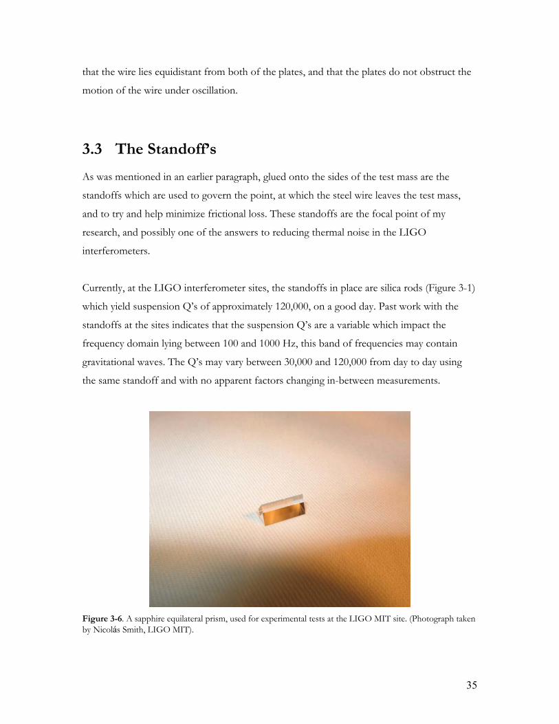
Currently, at the LIGO interferometer sites, the standoffs in place are silica rods (Figure 3-1)

which yield suspension Q’s of approximately 120,000, on a good day. Past work with the

standoffs at the sites indicates that the suspension Q’s are a variable which impact the

frequency domain lying between 100 and 1000 Hz, this band of frequencies may contain

gravitational waves. The Q’s may vary between 30,000 and 120,000 from day to day using

the same standoff and with no apparent factors changing in-between measurements.

Figure 3-6. A sapphire equilateral prism, used for experimental tests at the LIGO MIT site. (Photograph taken by Nicolás Smith, LIGO MIT).

35

The goal of the experiment is to produce a reproducible high, consistent Q measurement by

adjusting how the wire is clamped to the test mass. The results would impact Scientific Run

6, Enhanced LIGO, with further application in Advanced LIGO for the auxiliary mass

suspensions.

The standoffs to be tested consist of grooved and un-grooved BK7 right angle prisms (BK7

is a hard bor-crown optical glass), sapphire prisms and silica rods. We also tested a clamp

standoff made from tool steel (a better description of it can be found in Chapter 4). The

grooved prisms all have an assortment of cuts (shallow or deep) indented into the edges,

created using whichever method is convenient and manageable for the material of the prism

(Figure 3-6). The sapphire and BK7 prisms were cut using both diamond-dust covered wire,

and a laser. The tool steel clamp was created to have a groove, like the clamps to the support

structure, to hold the wire in place.

Figure 3-7. An image of a groove cut by an Excimer laser into a BK7 prism. This image was taken with a camera microscope. (Photograph taken by Lucienne Merrill) We also tested an additional standoff, one which is smaller than the pre-ordered standoffs, as

a combination to the standoff set-up. This prism is made from Aluminum and much smaller

than the others; a better description of it can be found in Chapter 4. This prism was always

36

placed below the initial standoffs which were listed earlier, but never used in the tool steel

clamp orientation.

3.4 The Electronics For the purpose of the experiment there are some electronics which are used both in

vacuum and in air for measurements, as well as those that are used strictly in vacuum and

those used strictly in air. The reason some measurements are taken under vacuum, while

others in air, all depends on whether we are trying to simulate the actual environment for a

LIGO test mass or if we are trying to calibrate the test mass for a new experiment. The most

crucial measurements for this experiment are a result of the steel chamber being in a

vacuum. However, the only major difference between in air and under pressure

measurements is the driver which is used to push the wire into oscillation.

3.4.1 Magnetic Driver In order to determine the resonance, characterize and retrieve the force on the wire in air

without electric breakdown before pumping down, we use a magnetic driver. While the

apparatus is in air, a magnetic driver is set up and situated next to the wire (Figure 3-7). The

magnetic driver is powered by a 0~20V power supply (0.5 A), and controlled with a Type

2760 Power Amplifier with a maximum output of 40 dB with gain. This driver is set up

electronically so that its input to the wire is controlled by one of two methods: either its

input is controlled using the correct frequency of the wire and a fixed sine wave, or it is set

up using a Lock-In amplifier, which uses a range of frequencies to initiate oscillation in the

wire (this range is usually set between 280 and 340 Hz, to measure first harmonics). The

output of the magnetic drivers is used in one of three different ways each time it is used to

drive the wire at resonance. Its output is either controlled using a positive feedback loop,

using the known resonant frequency of the wire to drive itself using ‘fixed sine’ on the Signal

Analyzer and by using white noise to drive the wire (normally used to determine the natural

frequency of the wire).

37

Steel Vacuum Chamber

Suspension Experiment

Figure 3-8. The bell jar - open and not under vacuum. (Photograph taken by Lucienne Merrill)

3.4.2 High Voltage Driver Once the bell jar is in vacuum, a Burleigh High Voltage DC Op Amp is set up to actuate on

the wires in the same fashion that the magnetic driver was set up. As was mentioned before,

the electronic drivers used under vacuum are the copper plates set up around the wires of

the test mass. The Burleigh can output up to 1.0 kV with 0-200 gain onto what it’s powering.

In this experiment, the high voltage supply is applied to the pair of copper plates. The wire

can be pushed in one of two directions at a time, both forwards and backwards or both left

and right, which are also the directions that the shadow sensors are sensitive to. The HV

(high voltage) is set up so that its input is governed by a grid of BNC (Bayonette-Neil

Concelman) cables connections. The grid consists of four choices: RLR (Right wire, Left-

Right), RFB (Right wire, Front-Back), LLR (Left Wire, Left-Right), LFB (Left Wire, Front-

Back), all of which are different directions that the wire can be pushed into oscillation.

Depending upon the desired direction of motion for the wire, the BNC cable flowing from

the HV can be connected to any one of those ports.

38

As was mentioned earlier, each wire has its own pair of copper plate actuators, as well as the

ability to charge and oscillate the wire in both polarizations. When the HV is applied to one

of the directions, say LFB, then one of the copper plates will get charged so that it will

attract the steel wire in the front back direction. This attraction results in a charged steel

wire, meaning that its next attraction will be to ground, so it moves towards the other

uncharged copper plate. As one can only guess, the attraction of the wire between the

charged and uncharged plates causes an oscillation, which surprisingly enough results in a

steady and convenient way to oscillate the wire.

3.4.3 Vacuum System During actual experimental tests, it is necessary to operate in vacuum as it is a way to avoid

buffeting by air molecules, which could lower the Q, and simulate the environment of the

test mass at the LIGO sites. The Qs for the wire vary greatly between in air measurements

and in vacuum, meaning, the Qs are only several thousand in air and around a hundred

thousand in vacuum. The vacuum system set up for the suspensions experiment can be seen

in Figure 2-8. There are three vacuum pumps available to the experiment, where two are

usually all that are needed for the vacuum to be under pressure at any point in time.

39

Roughing Pump

Turbo Pump

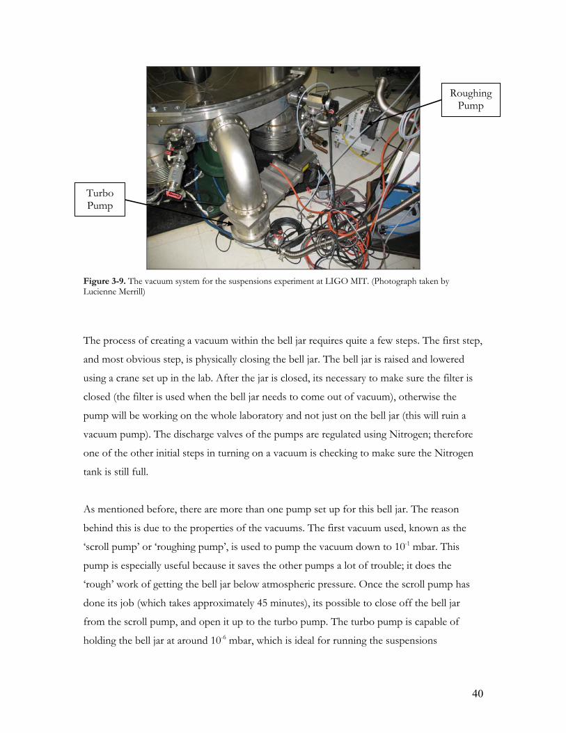
Figure 3-9. The vacuum system for the suspensions experiment at LIGO MIT. (Photograph taken by Lucienne Merrill)

The process of creating a vacuum within the bell jar requires quite a few steps. The first step,

and most obvious step, is physically closing the bell jar. The bell jar is raised and lowered

using a crane set up in the lab. After the jar is closed, its necessary to make sure the filter is

closed (the filter is used when the bell jar needs to come out of vacuum), otherwise the

pump will be working on the whole laboratory and not just on the bell jar (this will ruin a

vacuum pump). The discharge valves of the pumps are regulated using Nitrogen; therefore

one of the other initial steps in turning on a vacuum is checking to make sure the Nitrogen

tank is still full.

As mentioned before, there are more than one pump set up for this bell jar. The reason

behind this is due to the properties of the vacuums. The first vacuum used, known as the

‘scroll pump’ or ‘roughing pump’, is used to pump the vacuum down to 10-1 mbar. This

pump is especially useful because it saves the other pumps a lot of trouble; it does the

‘rough’ work of getting the bell jar below atmospheric pressure. Once the scroll pump has

done its job (which takes approximately 45 minutes), its possible to close off the bell jar

from the scroll pump, and open it up to the turbo pump. The turbo pump is capable of

holding the bell jar at around 10-6 mbar, which is ideal for running the suspensions

40

experiment. The experiment only requires that the pressure be below 10-4 mbar, for no effect

on the Q, however, we normally wait to make measurements until it is around 10-5 mbar.

3.4.4 Data Recording A computer program was created to monitor and record the decay of the oscillation in the

wires so that determining the Q of the wire in a particular set up (different clamp, different

standoff, etc.) was particularly easy. The program made for an experimental set up measuring

decay times, was created by Andri Gretarsson a former graduate student from Syracuse

University, specifically for the purpose of retrieving the exponential decay of the wire.

This program, known as AcquireV, takes the filtered signal from the wire and records it

according to the parameters set up in the program. If desired, both of the polarizations of

the wire can be recorded; that is, the front back and left right channels from the sensors

can be recorded into AcquireV. The time as well as the amount of scans that the program

takes from the decay can be adjusted, and normally are set up so that it measures between

two and four minutes, with a sample rate of 5000 and the number of scans per sample

equal to 600,000.

Two different methods were used to analyze the data from AcquireV. The methods were

two different Matlab programs, created after AcquireV to analyze the decay of the

oscillation, and output a Q measurement. One of the Matlab files entitled ‘Qfit.m’ was

created by Steve Penn (and more), and the other, a full bandwidth program, entitled

‘Plotenergy.m’, created more recently, by Matt Evans. Both of the Matlab files require

the location of the file on the computer and the frequency at which the wire resonates,

however one of the programs asks, more specifically, for the sensitivities of the sensors

used to watch the natural decay of the wires oscillation. These sensitivities varied, as

mentioned in Section 3.2, depending upon the wire and the direction of excitation.

All of the Q’s that are a result of this experiment were measured and recorded using these

programs.

41

3.5 Alignment and Calibration In order to reveal consistent, repeatable results, it is necessary to have a reliable experiment;

this next section details the work done on the suspensions experiment to create a reliable

structure and experiment. The steps taken to ensure reliability from the experimental set up

required proper alignment of the test mass and standoffs, sensor calibration, testing for

recoil in the structure, damping the pendulum swing, and testing for ‘creaking’ in the wire

(broadband noise).

3.5.1 Test Mass Alignment There are several degrees of freedom of motion for a pendulum subject to an external force.

The reason to restrict all of these motions is obvious for this experiment; the modes of the

test mass are not the object of experimentation, instead it is the wire and its violin modes.

The pendulum’s swing could interact and potentially lower the Qs of the wires, as the

coupling of a system with a lower Q to that of a higher Q would produce a Q closer to the

value of that of the lower. Figure 3-9 shows the degrees of freedom for a single loop test

mass.

Figure 3-10. The LIGO pendulum suspension, indicating all directions of motion (degrees of freedom)[6].

In Figure 3-9, the front view, 2b is the distance between the placements of the standoffs on

the test mass. The roll of the test mass within its steel wire holder is given by (; the length

of the steel wire from the point at which it leaves the test mass to the clamps (or its support

42

structure of any kind) is given by l, with the distance between its connections at the top by

2a. The other two diagrams are pretty self-explanatory, except it is necessary to point out )

and *, which are the pitch and yaw, respectively. These are the two motions which bear

much grievance when it comes to hanging the test mass, as they are the easiest motions to

instigate.

The yaw of the pendulum happened to become a problem at one point during the

experiment. This issue was resolved using a quick interpretation of Lenz’s law; using a strong

magnet and a small slab of aluminum. A tiny neodymium magnet was taped, using double

sided tape, onto the very bottom of the pendulum, at a distance H from the edge of the

bottom (referring to Figure 3-9, top view), and a piece of aluminum from an optics table was

placed below the magnet onto the bottom of the support structure. There was a hole in the

piece of aluminum and it was situated under the magnet so that the magnet hovered just

above it. The motion of the pendulum would be damped by the friction between the magnet

and the rest of the clamp.

There is already little to no motion of the pendulum in the ( direction (the roll). This is a

very hard motion to instigate, it requires a lot of force; the pendulum does weigh 10.5 kg

and is held in place with the single loop wire, clamped at the top and also held in position by

the standoffs.

The pitch, motion in the ! direction (seen in Figure 3-9 in the side view), is reduced to little

or no motion by the ability to hang the test mass correctly. If the test mass does not sit

correctly in the wire, then it is subject to a pitch. The wire has to loop around the test mass

at exactly the midpoint of its width in order to prevent any pitch. If the test mass continues

to pitch, which at one point during the experiment it was unrelenting, then one way to cure

it is to offset the pitch by adding weight to the raised section of the test mass. This is exactly

what was done at one point. A series of masses, intended for weighing, were taped using

vacuum compatible tape, to the top of the test mass at the edge which was tipping upwards

(Figure 3-10). Unfortunately, the test mass did not look anywhere near as beautiful as it did

when the experiment began a few months prior, but at least the pitch was gone.

43

Another part of the test mass alignment is the location of the standoff. If the stand off is

glued or even just placed onto the side of the test mass it could cause the whole test mass to

pitch. See Figure 3-10 for a picture of the wire in the standoff.

Figure 3-11. A picture of the wire placed midway along the width of the pendulum. (Photograph by Lucienne Merrill)

In order to ensure the proper alignment of the test mass, reduce the pitch, and guarantee a

consistent experiment where we wouldn’t have to change to wire, it was necessary to create a

method of hanging the pendulum which would does just that. An aluminum rig was created

that would raise the test mass to the same height every hanging. The rig is pretty simple, and

it sits underneath the whole test mass throughout all experimentation.

3.5.2 Recoil Another problem which had to be addressed was whether or not the structure was

experiencing recoil. Recoil means that whenever the wires are excited, the structure

experiences vibrations, causing the Q of the wires to be lower than it would normally be

because the mechanical loss of the cage is worse than that in the wire.

The test for recoil was relatively simple; it only required exciting the wire and sensing all

motions using a seismometer. The resulting signal from the seismometer was read on the

44

Signal Analyzer, and any excitations other than that from the wire could be seen as large

peaks above the noise level.

The seismometer is an extremely sensitive piece of equipment, and it is a lot more sensitive

to the motion of the wire and the structure than the shadow sensors can see. The recoil

energy versus the wire energies can be found in the table below:

WIRE RFB RLR LFB LLR

structure

wire

EE

4 x 104

1 x 105

8 x 104

4 x 105

Table 3-2. Recoil energy ratios between the wire and support structure.

We tried several tests to eliminate the obvious recoil within the structure, but were

unsuccessful. The first test that we tried involved adding more mass to the support structure;

this did not change the ratios above significantly. Secondly, we tried adding steel arms to the

structure, such that they clamped down the structure to the optics table. This proved a

useless effort as well.

After these tests, directing the seismometer in all polarizations to test for all sensitivities, it

was determined that there was no fixable recoil in the structure that was affecting the

excitation of the wire in air, and therefore no fix for the system under vacuum.

3.5.3 Wire Creaking The idea of wire creaking is a more recent revelation; the idea that the wire was moving

around in its groove on the prism would mean that the wires oscillation was losing energy,

being damped, and causing a lower Q (Figure 3-12). The damping of the oscillation was

thought to be lost in the section of wire just below the standoff, and this was another

function of the stylus, to see what the energy of oscillation was below the prism as compared

to the energy of oscillation of the wire above the prism (where it was actually being driven).

45

Clamp

Potential Motion below standoff

Standoff

Figure 3-12. Motion of wire above and potentially below standoff in suspension apparatus.

If the wire were “creaking” in its place on the prism, then this noise, ideally, would be heard

across the test mass, including the ‘unspeakable’ section of wire just below the standoff. This

noise is known as “up-conversion” or “broad-band noise”, and resembles a 1/f dependence

on the signal analyzer in the noise.

The process of testing for broadband noise involves creating a motion sensor, to detect the

slightest vibrations all over the test mass/wire, which may indicate up-conversion. This up-

conversion would appear as to level off, above the normal noise of the system. To test for

this, we created an apparatus to test for up-conversion using a needle from a phonograph

machine and an optics translational stage, called ‘the stylus’. The needle is the most

important part of the apparatus, the amplifier for the stylus is operated using ±12 volts and

its output is read on the Signal Analyzer. The “stylus” was made so that the phonograph

needle could sit vertically against the test mass, the opposite direction to which it was

originally intended for when it was made for phonographs.

46

The actual test for motion below the wire, and thereafter up conversion, involved placing the

stylus on different locations on the wire. The stylus tip was situated on the wire-prism

contact point, below the prism in several places, and below the aluminum prism (the second

standoff, when it was in place). The calculated ratios for the motion of the stylus versus the

motion of the stylus, therein the total amount of motion felt below the prism, or both the

prisms (depending upon the test) can be found in the appendix.

The wire above the prism standoff was excited at different levels, and the resulting data was

saved as ASCII code from the Signal Analyzer. This data contained all of the peaks and

valleys indicated in the figures below, and their corresponding frequencies. The frequency

range was set up to measure between 250 Hz to 1.05 kHz, and the amplitude varied as

indicated.

In the process of gathering the data from the stylus, it is necessary to make a few notes on

the actual circuitry set up for the stylus. The data retrieved from the stylus is initially filtered

using a Twin-T filter (you can find its circuitry design in the Appendix), and a High-Pass

filter (schematic circuitry design also found in the Appendix). The Twin-T was created to

filter the resonant frequencies, which, in our case, occurred at 292 Hz. If there were no drive

present at all, the Twin-T would produce a huge dip in the noise spectrum shown on the

Signal Analyzer right at 292 Hz, and this dip in the spectrum has a bandwidth of about 2 Hz.

The High-Pass filter, which is designed to do just as its name suggests, filters out all

frequencies above a certain frequency, namely ones that we don’t care about, those greater

than 1.05 kHz.

One of our first tests involved measuring the motion below the BK7 prism standoff, with no

extra standoff below it. This was to see if there was transmission to the test mass by the

slope of the wire not being constrained. As a result, the graph below shows the motion

beneath the prism standoff:

47

Figure 3-13. Wire motion and up-conversion below the BK7 prism standoff with no aluminum prism.

The legend on the left of the graph indicates which color corresponds to the level the wire,

above the standoff, was driven at using the fixed sine source from the Signal Analyzer. The

dramatic separation between the levels of the noise while the wire is not being driven and

while the wire is excited is the sign of up-conversion. Note the leveling of the noise along an

almost horizontal axis as compared to the slope of the natural floor of the system with

where the wire isn’t being excited at all.

We also tested the up-conversion, and motion of the wire as a result of placing the

aluminum prism beneath the prism standoff, as an added constraint to try and restrict

motion beneath the prism. The results indicated that up-conversion was still there, and as a

result motion was still being lost beneath the initial prism standoff, however it was decreased

by adding in the position constrains indicated that up-conversion was still there, and as a

48

result motion was still being lost beneath the initial prism standoff, however it was decreased

by adding in the position constraint.

Figure 3-14. Observed motion of wire with Sapphire prism and aluminum prism set-up.

The area in between no excitation and the excitations of the wire, Figure 3-13, indicates that

there is still slight up-conversion, and motion being lost beneath the first prism. This area is

much smaller than it was in the previous investigation, where there was no extra constraint

in the area below the main prism standoff. The levels at which the wire were excited in the

figure above are given in cm·rms, these levels are the displacements of the wire at the

different excitations in the area above the initial prism standoff. The results from the stylus

given in the figure show the resulting displacement of the wire below the standoff, in

comparison to the displacement of the wire above it. This tells us that there is still motion

being lost below the standoff, though it has been dramatically decreased.

49

We then decided to test the motion of the wire beneath the aluminum prism, the second

standoff, to see if there is any motion beneath it.

Figure 3-15. Motion of wire beneath Aluminum prism.

As one can see in Figure 3-14, there is absolutely no up-conversion and thereafter, no

apparent motion beneath the aluminum prism. This result indicates that the aluminum prism

restricts motion between it and test mass, reducing the friction to almost null with the wire

and test mass during oscillation.

On the other side of the test mass, during these tests with the standoffs, we had the tool

steel clamp glued on. We decided to test the up-conversion with that orientation, and also

we decided to use the stylus to test to see if we were losing any energy, if any motion was

being translated, to the glue between the test mass and the clamp.

50

Figure 3-16. Motion of the clamp during wire excitation.

The motion of the clamp as a result of the excitation of the wire is similar to that of the area

beneath the aluminum prism. The lack of distinction between the motion while exciting the

wire and not indicates that there is no up-conversion.

The energy lost in the glue between the test mass and the clamp was calculated to be ~10-3,

which is a very small amount lost and can be considered negligible. Therefore, gluing the

clamp onto the test mass does not add to any loss already associated with the wire

suspensions system.

51

Chapter 4

Experimental Results Recall that the motivation for this research lies in the excess and inconstant loss which has

been observed in the test mass violin modes at the sites and in several experimental

suspensions tests over the past years. This excess loss is suggested by several results

containing inconstant wire Q values. This loss is thought to arise from poorly defined

boundary conditions of the wires on the test mass, initially defined by a simple silica rod

standoff.

The experiments test the theory that the standoffs, used to define the point at which the wire

leaves the test mass, are the reason for excess wire dissipation. In this section we provide an

overview of the results for the standoffs and the use of an additional position constraint

which were performed between September 2007 and May 2008 on the test mass in the

LIGO lab at MIT. Each section of this chapter will focus on the different types of standoffs

that were tested in the experimental suspension at MIT: BK7 prisms, Sapphire prisms, fused

Silica rods and tool steel clamps.

Each of the separate experiments involved changing the standoff from one of the sides of

the test mass. During experimentation, it usually happened that one standoff on one side of

the test mass remained the same while the other side changed frequently. This way the

results from one side would, ideally, stay consistent, while the other side would be changing.

Also, some of the standoffs were glued on, and some were not. These factors will be

indicated in the section where they occur.

52

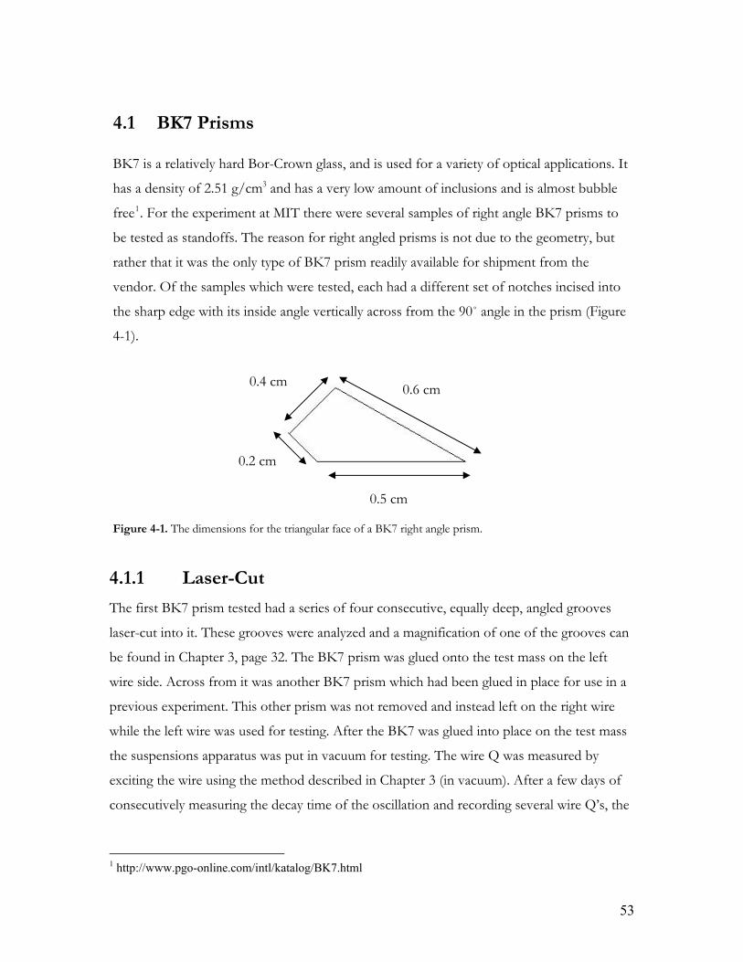
4.1 BK7 Prisms BK7 is a relatively hard Bor-Crown glass, and is used for a variety of optical applications. It

has a density of 2.51 g/cm3 and has a very low amount of inclusions and is almost bubble

free1. For the experiment at MIT there were several samples of right angle BK7 prisms to

be tested as standoffs. The reason for right angled prisms is not due to the geometry, but

rather that it was the only type of BK7 prism readily available for shipment from the

vendor. Of the samples which were tested, each had a different set of notches incised into

the sharp edge with its inside angle vertically across from the 90 angle in the prism (Figure

4-1).

0.4 cm 0.6 cm

0.2 cm

0.5 cm

Figure 4-1. The dimensions for the triangular face of a BK7 right angle prism.

4.1.1 Laser-Cut The first BK7 prism tested had a series of four consecutive, equally deep, angled grooves

laser-cut into it. These grooves were analyzed and a magnification of one of the grooves can

be found in Chapter 3, page 32. The BK7 prism was glued onto the test mass on the left

wire side. Across from it was another BK7 prism which had been glued in place for use in a

previous experiment. This other prism was not removed and instead left on the right wire

while the left wire was used for testing. After the BK7 was glued into place on the test mass

the suspensions apparatus was put in vacuum for testing. The wire Q was measured by

exciting the wire using the method described in Chapter 3 (in vacuum). After a few days of

consecutively measuring the decay time of the oscillation and recording several wire Q’s, the

1 http://www.pgo-online.com/intl/katalog/BK7.html

53

average Q was 71,600 with a standard deviation of 8,350 (for the full range of wire Q values

measured with this prism, see Appendix A).

The result of the initial BK7 tests indicated that we needed to move on and test another

prism. The first BK7 was removed from the left side of the test mass, using methanol and a

razor to remove it, as well as any residual glue on the test mass.

The next tests involved another BK7 right-angle prism with a different set of grooves laser-

cut into it. The grooves on this prism were labeled 1, 2, 3, and 4 in order of depth. That is

to say, that groove 1 was the shallowest groove and groove 4 was the deepest. Only grooves

1 and 2 were tested on this prism. The prism was, again, glued onto the test mass. The

results from the different grooves on this BK7 prism were worse than those found with the

first BK7 prism. The average Q for groove 1 on this prism was 30,000 and the average Q

for groove 2 was 81,100. Between the grooves this seems like an improvement, however the

range of Q’s for groove 2 went from 60,000 to 90,000 which show just how inconsistent the

Q’s were.

4.1.2 Un-cut As was mentioned earlier, the other prism on the test mass during experimentation with the

other BK7 prisms was another BK7 prism. This prism had been glued onto the test mass,

on the right wire side, for at least a month before experimentation with the standoffs had

been undertaken. This prism had been placed onto the test mass initially with no groove cut

into it. However, after a month of suspension, the wire had cut its own groove into the edge

of the BK7 prism, providing us with another type of standoff to test. The results of the

BK7 prism were spread out across a nice range, as with the results of the laser-cut BK7,

groove 2. The average Q was 82,500 with a standard deviation of 11,650 (quite a large

variation in data).

Despite the poor Qs of the BK7 prism, positive results did eventually flourish from initial

experimentation with this prism standoff. The idea, which came later in the year, was that

the wire below the prism was vibrating during excitation of the wire above the prism. This

54

would intrinsically lower the Q values, as it means that the energy in the oscillation of the

wire was being lost to the area below and as a result there was added friction between the

wire and the test mass. The solution, which was developed by Rai Weiss, involved adding

another prism, below the BK7 prism to define the boundary conditions between the wire

and the test mass much better than before, in an attempt to minimize (if not eliminate) any

friction and energy loss witnessed before.

The position constraint was made from a piece of scrap aluminum, with no approximate

dimensions in mind but only that it had to be smaller than the actual prism standoff. The

prism was cut by Nicolás Smith, a graduate student at MIT. When the piece had been cut,

its base measured 3 x 3 x 2.5 mm with a length of 7mm. The aluminum prism was placed

below the BK7 standoff and glued onto the test mass (not onto the wire) at a point under

the BK7 prism where it felt taut (Figure 3-2).

Prism Standoff

Al prism

Figure 4-2. A side view of a prism standoff above the aluminum position constraint. Photograph taken by Lucienne Merrill.

55

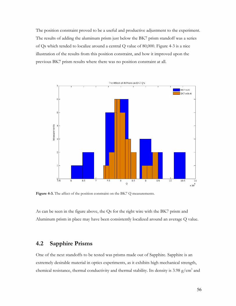
The position constraint proved to be a useful and productive adjustment to the experiment.

The results of adding the aluminum prism just below the BK7 prism standoff was a series

of Qs which tended to localize around a central Q value of 80,000. Figure 4-3 is a nice

illustration of the results from this position constraint, and how it improved upon the

previous BK7 prism results where there was no position constraint at all.

Figure 4-3. The affect of the position constraint on the BK7 Q measurements.

As can be seen in the figure above, the Qs for the right wire with the BK7 prism and

Aluminum prism in place may have been consistently localized around an average Q value.

4.2 Sapphire Prisms One of the next standoffs to be tested was prisms made out of Sapphire. Sapphire is an

extremely desirable material in optics experiments, as it exhibits high mechanical strength,

chemical resistance, thermal conductivity and thermal stability. Its density is 3.98 g/cm3 and

56

can be cut into prisms, like the BK7 and grooved using a laser and/or diamond covered

wire. The sapphire prisms were geometrically different from the BK7 prisms, as they were

cut into equilateral prisms, the dimensions for these prisms and their design can be found in

Figure 4-4, below.

Figure 4-4. Dimensions of equilateral Sapphire prisms [31].

Three different types of Sapphire prisms were tested on the suspension apparatus: a

sapphire prism with no grooves, one with grooves cut with a laser and the other with

grooves cut using diamond-dust covered wire.

4.2.1 Un-cut The first Sapphire prism to be tested had no grooves cut into its edges at all. However,

while hanging the test mass the prism was chipped slightly at the very tip where the wire sat.

The force from the wire against the standoff was too great on such a small area and the wire

got away with cutting into its edge. The groove wasn’t terribly deep, but could have affected

the results. However, if LIGO ever wanted to potentially use Sapphire prisms with no

groove cut into them, then they would experience the same problem, therefore the results

from this particular experiment are still valuable.

57

This individual sapphire prism produced lower Qs than were anticipated. The initial

thoughts were that the sapphire would be a good contestant as compared with other

standoffs because of its good materialistic properties. The sapphire was situated onto the

test mass, but not glued onto the test mass, as a test to see if it increases the Q. The results

showed dismal Q values, with an average Q of 53,000 and a standard deviation of 15,000.

These results led us to conclude that the standoffs do need to be glued onto the test mass,

and after this test, all of them were.

4.2.2 Laser Cut The next sapphire prism which was tested had its groove cut by a laser. This groove was cut

to the size of the wire, but not deep enough to encase the wire. The drawing sent to the

manufacturer to have the prism cut, and the dimensions required, can be found in the

Appendix. The BK7 prism which had been on the right side of the test mass for several

months was removed, and replaced with the laser cut sapphire prism. This prism was glued

on and below it we placed the aluminum prism position constraint. The Q’s measured from

this set up were the best Q’s measured with a prism in the suspension apparatus, all

concentrated around an average Q of 118,000 and a standard deviation of 7,000.

The Q’s from the laser cut sapphire prism are remarkably higher than the values for any of

the other prisms tested in this apparatus. This means there is less loss in this set up than in

any of the other ones so far, and this result could be an improvement on the suspension

thermal noise in the next generation of interferometers.

4.2.3 Diamond-Dust Wire Cut The last type of sapphire prism to be tested in the suspension set up is one with grooves cut

using a wire coated with diamond dust. It was suggested to us that we should try making a

constraint using a wedged groove in a Sapphire prism (which we had just shown to be a

good option in the suspensions experiment) to grab the wire. We made the groove using a

steel lath in the shape of the groove and diamond powder was put on the lath. The idea

governing this test was that the wire would be restricted from moving around in its groove.

58

The grooves which have been cut into any of the prisms so far have been just deep enough

for the wire to sit in them, but not deep enough to keep the wire from twitching around.

This sapphire prism was glued onto the right side of the test mass, taking over the area

where the laser cut sapphire prism had been before. When the test mass was hung the wire

was fit into the groove of the prism, and it couldn’t come out, which is what we wanted. The

aluminum prism was also fit under the prism, per routine now, and glued into place as well.

After putting the set up in vacuum, and measuring Q’s, the initial results showed us right

away that this particular set up was not what we were looking for. The average Q was 64,800

with a standard deviation of 5,000. Despite the consistency of the results, which could be

attributed to the position constraint, the Q’s indicate that this particular set up is not ideal in

minimizing the excess dissipation in the suspensions.

A view of all of the results from the sapphire prisms can be seen in the histogram below,

with the laser cut sapphire being the only results so far where the Q has increased

drastically, indicating that the dissipation in the suspensions had been improved (Figure 4-

5).

59

Figure 4-5. Complete distribution of Q measurements for all of the sapphire prisms tested.

4.3 Tool Steel Clamp The next, most interesting, standoff to be tested on the suspension apparatus is a clamp.

The clamp is made from tool steel, a carbon alloy which is a soft metal that can be heat

treated into a hard metal. The clamp was created with a groove right down the middle of it,

with two pins on either side of the groove (Figure 4-6). The groove was supposed to encase

the wire, and clamp it into place onto the test mass. A schematic drawing of the dimensions

of the clamp by Rai Weiss can be found in the Appendix.

Figure 4-6. The size and layout of the tool steel clamp.

The clamp was situated on the left wire side of the test mass, and it was screwed together

once we were sure that the wire was sitting in its groove. It was glued onto the test mass

(Figure 4-7) and we measured the Q’s as a result on the left wire side of the test mass, in

vacuum.

60

Figure 4-7. The clamp situated and glued onto the test mass, in place of a normal standoff.

The Q measurements of the first trial with the clamp were remarkable. The values that were

being measured are comparable to those measured with the laser cut sapphire and aluminum

prism set up; however, these values are even more localized around a central average. The

average Q was 119,000 with a standard deviation of 2,300.

One idea, which was mentioned earlier in Chapter 3, was that there may be energy loss as a

result of gluing the clamp to the test mass (energy loss in the glue). It was calculated that

there was hardly any energy lost in this orientation, however we wanted to test this theory

experimentally to prove the theory; so, we added more glue to the already glued on clamp to

see the affect it had on the wire Q.

The wire Q actually increased, very small increase, as a result of adding more glue to the set-

up. The measured wire Q’s from this new arrangement had an average value of 121,000 now,

with a standard deviation of 1,500.

4.4 Initial LIGO Standoffs The motivation in this research lies within the excess and inconstant wire dissipation in the

Initial LIGO suspensions, whose wire to test mass boundaries are defined by grooved, silica

rod standoffs. However one may choose to look at the data as a result from earlier

experiments, we decided to test the inconsistencies and low Q values which have become

associated with the silica rods.

61

We managed to retrieve a silica rod, an exact replica of the ones in the current LIGO

suspensions, and we replaced the sapphire prism on the right side of the test mass, with the

silica rod. The silica rod was glued onto the test mass, and the aluminum prism was glued

beneath it. The LIGO suspensions do not actually have an aluminum prism as a second

boundary for the wire, but we decided to test the wire Q values with and without it, and the

set up with the aluminum prism was decided upon to test first.

The Q measurements, as usual, were done in vacuum, and the results showed a consistent Q

value of 88,000 as a result of exciting the wire in both the front-back and left-right

polarizations. While exciting the wire, and accumulating data, it appeared that when the wire

was being excited front-back, energy was being coupled between the motions of the wire.

That is to say, some of the energy from the front-back was going into left-right, and vice

versa, and this appeared on several energy plots as a severe beating pattern (Figure 4-8).

Figure 4-8. Energy decay for RFB excitation with silica rod standoff.

62

To the contrary, when the wire was excited in the left-right direction, there appeared to be

no coupling at all (Figure 4-9).

Figure 4-9. Energy decay for RLR excitation with silica rod standoff.

This beating pattern may be indicative of what was seen the sites as well, and perhaps a

reason for inconsistencies. The aluminum position constraint may be the only reason why

the Q values are consistent, without it, perhaps the reason for the variety of Q values seen

before.

The Q’s for the silica rod standoff with the aluminum prism were recently measured at the

MIT LIGO site, and the results can be found below. No tests have been done so far to

compare the silica rod standoff without the aluminum position constraint, so we will rely on

the previous data taken by Gregg Harry and Steve Penn to compare our results with. Figure

4-10 shows an improvement on the inconstant wire Q of the silica rod standoff results

using the aluminum prism, as compared with the distribution of wire Q’s without it.

63

Figure 4-10. Initial LIGO Silica Rod results with and without Aluminum prism.

64

Chapter 5 Conclusion We end this paper with a summary of results and several proposals for future work regarding

thermal noise in the LIGO suspensions.

5.1 Summary As a result of testing several standoffs in an attempt to improve an observed energy loss in

the suspension wires of the LIGO interferometers, we present three solutions to improve

the thermal noise for Enhanced LIGO.

If LIGO decides to keep the grooved silica rod standoffs, or chooses to exchange them with

a prism standoff, then a solution to the inconsistent dissipation in the suspension wires

would be to constrain the slope of the wire with the test mass with a second standoff. This is

probably the easiest and most affordable in terms of time and money.

The second solution, which would not only improve the consistency in the suspension wires,

but it, would also improve upon the dissipation in the system. This solution requires

exchanging the silica rod standoff used in the current LIGO suspensions with the laser cut,

equilateral, sapphire prism and beneath it the aluminum prism. The results from the

experiment were incredibly consistent and the energy loss was minimized by about 30%. Of

all of the prisms that we tested, the sapphire was the only material which broke apart in

slivers, if at all, from its contact with the wire. The other prisms and rods, after analysis

under a microscope, broke apart in the grooves in chunks (Figures 5-1 and 5-2), which we

think is a reason for the difference in wire Q’s between the different materials.

65

wire

Chunks of BK7 or Silica

Figure 5-1. Abrasion of Silica and BK7 from contact with wire.

Wire

Slivers of Sapphire

Figure 5-2. Abrasion of Sapphire prisms from contact with wire.

Both figures above are exaggerations of the actual result from contact with wire, but the

abrasions indicated in the drawings are what have been seen after close analysis with a

microscope.

The only difficulty with this set up is the exchange of standoffs, and ensuring that when the

prisms are glued onto the test mass, there is no glue between it and the test mass. This

solution is far less invasive in the LIGO suspensions than the next solution we are going to

propose.

The third and final solution for improving the excess and inconsistent wire dissipation in the

LIGO suspension wires is the tool steel clamp. The tool steel clamp does not require an

additional position constraint to improve the slope coupling between the wire and test mass;

it is as capable of improving the suspension wires in LIGO as the Sapphire laser-cut prism

66

with aluminum prism is. Like the sapphire prism, it also improved upon the energy loss in

the system by 30%. The only difficulty with this standoff is that it, like the sapphire prism,

requires that the current LIGO test masses would have to be handled and the standoff

exchanged with a clamp. The clamp is far more invasive to the test mass than the Sapphire

prism is, and it would also have to be glued onto the test mass with no excess glue between

it and the test mass, though glue would be required and as we showed before, the glue does

not cause any additional energy loss in the suspension wires.

The total results of the experiment conducted at MIT can be seen below in Figure 5-3.

Figure 5-3. Total distribution of Q’s for the different standoffs used on the experimental suspension at MIT.

The results of this work can be compared to the work done by Gregg Harry and David

Malling, shown in Chapter 2. Our results show an improvement on consistency and value as

compared with their work.

67

5.2 Future Work As can probably be surmised from the results and conclusions, there seems to be a

fundamental limit to how much we can actually improve upon the energy loss in the

suspension wires at the MIT experiment. That is to say, two separate, distinctly different

standoffs each obtain consistent wire Q’s of ~120,000, but no higher.

This limit could be a result of the support structure for the suspensions experiment at MIT.

If so, then it would be interesting and valuable to the results of this paper, to find what is

keeping the Q’s of the suspensions from reaching material limit. If and when this is solved

for, the standoff’s could be tested again (primarily the laser cut sapphire and tool steel

clamp), to see whether or not they were limited by something other than their own material

properties.

The results provided in this paper offer improvements for the Enhanced LIGO suspensions,

and these improvements could also apply to Advanced LIGO. These results could be useful

for the auxiliary test masses in the Advanced LIGO multi-mass suspension systems.

68

Appendix A

Measured Q’s All of the Qs listed in the following tables were measured at the LIGO MIT facility between

September 2007 and May 2008. Also, it should be noted that each of the frequencies

recorded per Q are at the fundamental frequencies (first harmonics) for the wire. The

different polarizations used to drive the wire are listed as RLR, RFB, LLR or LFB

accordingly.

A.1 Q Measurements

Standoff Mode Q BK7 No Al LLR 8.12E+04

LLR 5.39E+04 LLR 6.94E+04 LLR 7.44E+04 LLR 8.06E+04 LLR 7.13E+04 LLR 6.64E+04 LLR 7.05E+04 LLR 7.71E+04 LFB 8.28E+04 LFB 9.58E+04 LFB 1.26E+05 LFB 1.34E+05 LFB 6.47E+04 LFB 3.00E+04 LLR 5.30E+04 RFB 1.06E+05 RFB 9.10E+04 RFB 1.02E+05 RLR 8.80E+04 RLR 9.60E+04 RLR 7.70E+04

69

RLR 7.70E+04 RLR 9.20E+04 RFB 9.40E+04 RLR 8.30E+04 RLR 7.90E+04 RFB 7.80E+04 RFB 6.00E+04 RFB 6.50E+04 RLR 6.50E+04 RFB 7.73E+04 RFB 7.90E+04 RFB 7.79E+04 RLR 8.17E+04 RLR 8.23E+04 RLR 8.07E+04

BK7 with Al RFB 8.20E+04 RFB 8.00E+04 RFB 8.10E+04 RLR 8.40E+04 RLR 8.40E+04 RFB 8.10E+04 RFB 7.90E+04 RFB 9.50E+04 RFB 9.40E+04 RFB 8.90E+04 RFB 8.50E+04 RLR 7.70E+04 RLR 8.50E+04 RLR 9.20E+04 LFB 1.20E+05 RLR 7.90E+04 RFB 7.80E+04 RFB 8.10E+04 RLR 7.80E+04 RLR 7.30E+04 RLR 7.70E+04 RLR 7.80E+04 RFB 8.00E+04 RFB 7.90E+04

70

Un-Cut Sapphire with

Al LFB

6.92E+04 LFB 3.67E+04 LFB 7.39E+04 LLR 4.77E+04 LLR 4.38E+04 LLR 4.65E+04

Laser Cut Sapphire with

Al RFB 1.34E+05 RFB 1.18E+05 RFB 1.19E+05 RFB 1.26E+05 RLR 1.08E+05 RLR 1.01E+05 RLR 1.16E+05 RFB 1.30E+05 RFB 1.21E+05 RFB 1.27E+05 RFB 1.21E+05 RFB 1.21E+05 LFB 1.11E+05 LFB 1.11E+05 LFB 1.08E+05 LLR 1.12E+05 LLR 1.19E+05 LLR 1.19E+05 LFB 1.08E+05 RLR 1.27E+05 RLR 1.18E+05 RLR 1.21E+05 RLR 1.12E+05 RFB 1.19E+05 RLR 1.16E+05 RFB 1.23E+05

Diamond Dust Wire Cut

Sapphire with Al RFB 6.22E+04

71

RFB 6.20E+04 RFB 6.03E+04 RFB 5.78E+04 RFB 5.71E+04 RFB 6.98E+04 RFB 7.11E+04 RFB 7.07E+04 RFB 7.12E+04 RFB 6.94E+04 RFB 6.58E+04 RFB 7.08E+04 RFB 6.69E+04 RLR 5.81E+04 RLR 6.24E+04 RLR 6.19E+04

Tool Steel Clamp LFB 1.19E+05

LFB 1.16E+05 LFB 1.17E+05 LLR 1.17E+05 LLR 1.17E+05 LFB 1.21E+05 LFB 1.17E+05 LFB 1.19E+05 LFB 1.17E+05 LLR 1.19E+05 LLR 1.20E+05 LFB 1.25E+05 LFB 1.20E+05 LFB 1.20E+05 LLR 1.21E+05 LLR 1.17E+05 LLR 1.21E+05 LFB 1.21E+05 LFB 1.19E+05 LFB 1.21E+05 LFB 1.19E+05 LFB 1.19E+05 LLR 1.20E+05

72

LLR 1.19E+05 LFB 1.16E+05 LFB 1.12E+05 LFB 1.16E+05 LLR 1.17E+05 LLR 1.17E+05 LLR 1.17E+05 LFB 1.18E+05 LFB 1.18E+05 LFB 1.20E+05 LFB 1.20E+05 LFB 1.20E+05 LFB 1.20E+05 LLR 1.21E+05 LLR 1.20E+05 LFB 1.17E+05 LFB 1.20E+05 LFB 1.23E+05 LFB 1.20E+05 LFB 1.22E+05 LLR 1.21E+05 LLR 1.23E+05 LFB 1.20E+05 LFB 1.21E+05 LLR 1.22E+05 LLR 1.17E+05 LLR 1.20E+05 LLR 1.22E+05 LFB 1.23E+05 LFB 1.21E+05 LFB 1.20E+05 LFB 1.22E+05

Silica Rod Standoff with

Al RFB 8.65E+04 RFB 8.36E+04 RFB 7.79E+04 RFB 8.63E+04 RLR 8.14E+04 RLR 7.79E+04

73

RLR 8.63E+04 RFB 8.60E+04 RLR 9.10E+04 RLR 9.83E+04 RLR 9.82E+04 RLR 9.67E+04 RLR 9.69E+04 RLR 9.62E+04 RLR 9.99E+04 RFB 9.91E+04 RFB 9.72E+04 RFB 9.40E+04 RFB 9.18E+04 RLR 1.01E+05 RFB 9.82E+04 RLR 9.36E+04 RFB 9.37E+04 RFB 9.30E+04 RFB 9.10E+04 RFB 8.80E+04 RFB 8.78E+04 RFB 8.88E+04 RFB 8.82E+04 RLR 8.78E+04 RLR 8.89E+04 RLR 8.74E+04 RFB 8.72E+04 RFB 8.72E+04

74

A.2 Dimensions of Clamp

A.3 Stylus Measurements These measurements were taken as mentioned in Chapter 3, and were converted into

centimeter displacements by assuming a gain of 200 on the PZT’s filter and a right wire

sensitivity: 2108.9 )+"cmVolts at the Nimbin output.

EXCITATION OF WIRE EXCITATION OF STYLUS x(stylus)/x(wire) Volts cm (pk) Volts cm(pk)

0.5 Vp 2.55E-02 2.28 1.14E-04 4.40E-03 1 Vp 5.10E-02 4.17 2.09E-04 5.70E-03

Below Prism No Al

2 Vp 1.02E-01 7.43 3.70E-04 3.60E-03

75

prism 5 Vp 2.55E-01 7.65 3.82E-04 1.50E-03 1 Vp 5.10E-02 1.83 9.15E-05 1.80E-03 2 Vp 1.02E-01 2.23 1.15E-04 1.10E-03

Below Prism No Al prism 5 Vp 2.55E-01 2.23 1.15E-04 4.50E-04

0.5 Vp 2.55E-02 0.67 3.35E-05 1.30E-03 1 Vp 5.10E-02 1.22 6.10E-05 1.20E-03 2 Vp 1.02E-01 1.94 9.70E-05 8.50E-04

On Prism No Al

5 Vp 2.55E-01 2.01 1.00E-04 3.90E-04 0.5 Vp 2.55E-02 2.44 1.22E-04 4.80E-03 1 Vp 5.10E-02 1.98 9.90E-05 1.94E-03

With Al

Below Prism 2 Vp 1.02E-01 2.12 1.06E-04 1.04E-02

0.5 Vp 2.55E-01 1.19 5.90E-05 2.30E-03 1 Vp 5.10E-02 1.22 6.10E-05 1.20E-03 2 Vp 1.02E-01 1.39 6.90E-05 6.70E-03

With Al On Prism

5 Vp 2.55E-01 0.87 4.30E-05 1.70E-04 1 Vpp 8.47E-03 0.34 1.70E-05 2.00E-03 2 Vpp 1.70E-02 0.91 4.50E-05 2.60E-03

With Al

Under Prism 7 Vpp 6.00E-02 3.65 1.80E-04 3.00E-03

0.5 Vpp 4.23E-03 0.196 9.80E-06 2.30E-03 1 Vpp 2.47E-03 0.415 2.07E-05 2.40E-03 2 Vpp 1.70E-02 0.694 3.50E-05 2.50E-03

On Prism With

Al 3 Vpp 2.58E-02 1.33 6.65E-05 2.60E-03

76

Bibliography

1 – G.M. Harry, S. Penn, A. Gretrasson, J. Betzweiser, S. Waldman, R. Weiss, “Suspension Thermal Noise in Initial and Enhanced LIGO”, LIGO-T070001-00-R, 2006. 2 - A. Gillespie, F. Raab, “Suspension losses in the pendula of laser interferometer gravitational-wave detectors”, Phys. Lett. A 190, 213-220 (1994). 3 - Joseph Kovalik and Peter R. Saulson, “Mechanical loss in fibers for low noise pendulums”, Rev. Sci. Instrum. 64 (10), Oct. 1993. 4 – Gabriela I. González and Peter R. Saulson, “Brownian motion of a mass suspended by an anelastic wire”, J. Acoust. Soc. Am. 96 (1), July 1994. 5 – S. D. Penn, A. Ageev, D. Busby, G.M. Harry, A. M. Gretarsson, K. Numata and P. Willems, “Frequency and surface dependence of the mechanical loss in fused silica”, Phys. Lett. A 352, 3-6 (2006). 6 – Gabriela I. González, “Suspensions thermal noise in the LIGO gravitational wave detector”, Class. Quantum Grav. 17, 4409-4435 (2000). 7 – A. M. Gretarsson, G.M. Harry, S. D. Penn, P. R. Saulson, W. J. Startin, S. Rowan, G. Cagnoli and J. Hough, “Pendulum mode thermal noise in advanced interferometers: a comparison of fused silica fibers and ribbons in the presence of surface loss”, Phys. Lett. A 270, 108-114 (2000). 8 – A. Gillespie and F. Raab, “Thermal noise in the test mass suspension of a laser interferometer gravitational-wave detector prototype”, Phys. Lett. A 178, 357-363 (1993). 9 – A. Gillespie, T. Lyons and F. Raab, “Near-Thermal Excitation of Violin Modes in the Test-Mass Suspension Wires of the 40-m Prototype Interferometer”, LIGO-T920006-00-R, 1992. 10 – A. Gillespie and F. Raab, “ An Investigation of Violin Resonances in the Test Mass Suspensions of the 40-Meter Mark I Prototype”, LIGO-T(no number on paper, will investigate) 11 – A. Abramovici, W. E. Althouse, R.W.P. Drever, Y. Gürsel, S. Kawamura, F. J. Raab, D. Shoemaker, L. Sievers, R. E. Spero, K. S. Thorne, R. E. Vogt, R. Weiss, S. E. Whitcomb and M. E. Zucker, “LIGO: The Laser Interferometer Gravitational-Wave Observatory”, Science, New Series, Vol. 256, No. 5055. (April 1992), pp. 325-333.

77

12 – B, Abbott, R. Abbott, R. Adhikari, B. Allen, et al., “Detector Description and Performance for the First Coincidence Observations between LIGO and GEO”, Elsevier Science, May 2006. 13 – Ohanian, Hans C. Gravitation and Spacetime. W.W. Norton & Company, Inc.: New York, 1976. 14 – Saulson, Peter R. “If light waves are stretched by gravitational waves, how can we use light as a ruler to detect gravitational waves?”, American Journal of Physics, Vol. 65, No. 6, June 1997 16 – Saulson, Peter R. Interferometric Gravitational Wave Detectors. World Scientific: New Jersey, 1994. 17 – Giancoli, Douglas C. Physics for Scientists & Engineers with Modern Physics, 3rd Edition. Prentice Hall: New Jersey, 2000. 18 – Kverno, Derek. “Oscillations and Resonance”, http://www.phy.davidson.edu/StuHome/derekk/Resonance/pages/Discussion.htm 25 - Saulson, Peter R. “Thermal noise in mechanical experiments”, Physical Review D, Particles and Fields, Third Series, Vol. 42, Number 8, October 15, 1990 26 - Adhikar, Rana. “Sensitivity and Noise Analysis of 4 km Laser Interferometric Gravitational Wave Antennae”, PhD, Massachusetts Institute of Technology, 2004. 27 - Harry, Gregg, “Thermal Noise in Initial LIGO”, LIGO-G050087-00-R, March 15, 2005. 28 - Weiss, Rai, “THE LIGO INTERFEROMETERS: How they work and how well they work”, LIGO-G030024-00-D, LSC AAAS Annual Meeting, Denver, Colorado, Feb 17, 2003 29 – Esham, Benjamin D., “A diagram of the Michelson–Morley experiment”, http://en.wikipedia.org/wiki/Image:Michelson-Morley_experiment_%28en%29.svg, December 4, 2007. 30 – Klimenko, S., Raab, F., Diaz, M., Zotov, N. “Violin Modes S2 Line Noise Investigation”, LIGO-G030130-00-Z, March 2003 31 – Communication with Rai Weiss, Nicolás Smith, Matthew Evans, Gregg Harry and Steve Penn. 32 – Weiss, R., Waldman, S., “Understanding Initial LIGO and Possible Influences on Enhanced LIGO”, PPT – February 2008

78