A study of the behaviour of linguistic fuzzy rule based classification systems in the framework of...
21
Fuzzy Sets and Systems 159 (2008) 2378 – 2398 www.elsevier.com/locate/fss A study of the behaviour of linguistic fuzzy rule based classification systems in the framework of imbalanced data-sets Alberto Fernández a , ∗ , Salvador García a , María José del Jesus b , Francisco Herrera a a Department of Computer Science and A.I., University of Granada, Spain b Department of Computer Science, University of Jaén, Spain Received 1 June 2007; received in revised form 17 December 2007; accepted 19 December 2007 Available online 31 December 2007 Abstract In the field of classification problems, we often encounter classes with a very different percentage of patterns between them, classes with a high pattern percentage and classes with a low pattern percentage. These problems receive the name of “classification problems with imbalanced data-sets”. In this paper we study the behaviour of fuzzy rule based classification systems in the framework of imbalanced data-sets, focusing on the synergy with the preprocessing mechanisms of instances and the configuration of fuzzy rule based classification systems. We will analyse the necessity of applying a preprocessing step to deal with the problem of imbalanced data-sets. Regarding the components of the fuzzy rule base classification system, we are interested in the granularity of the fuzzy partitions, the use of distinct conjunction operators, the application of some approaches to compute the rule weights and the use of different fuzzy reasoning methods. © 2007 Elsevier B.V. All rights reserved. Keywords: Fuzzy rule based classification systems; Imbalanced data-sets; Imbalance class problem; Instance selection; Over-sampling; Fuzzy reasoning method; Rule weights; Conjunction operators 1. Introduction Recently the imbalanced data-set problem has demanded more attention in the field of machine learning research [5]. This problem occurs when the number of instances of one class is much lower than the instances of the other classes. This problem is extremely important since it appears in many real application areas. Some applications in this field are the detection of oil spills from satellite images [28], identification of power distribution fault causes [47] and prediction of pre-term births [17]. Most classifiers generally perform poorly on imbalanced data-sets because they are designed to minimize the global error rate [27], and in this manner they tend to classify almost all instances as negative (i.e., the majority Supported by the Spanish Projects TIN-2005-08386-C05-01 and TIN-2005-08386-C05-03. ∗ Corresponding author. Tel.: +34 958 240598; fax: +34 958 243317. E-mail addresses: [email protected] (A. Fernández), [email protected] (S. García), [email protected] (M.J. del Jesus), [email protected] (F. Herrera). 0165-0114/$ - see front matter © 2007 Elsevier B.V. All rights reserved. doi:10.1016/j.fss.2007.12.023
-
Upload
alberto-fernandez -
Category
Documents
-
view
212 -
download
0
Transcript of A study of the behaviour of linguistic fuzzy rule based classification systems in the framework of...

Fuzzy Sets and Systems 159 (2008) 2378–2398www.elsevier.com/locate/fss
A study of the behaviour of linguistic fuzzy rule based classificationsystems in the framework of imbalanced data-sets�
Alberto Fernándeza,∗, Salvador Garcíaa, María José del Jesusb, Francisco Herreraa
aDepartment of Computer Science and A.I., University of Granada, SpainbDepartment of Computer Science, University of Jaén, Spain
Received 1 June 2007; received in revised form 17 December 2007; accepted 19 December 2007Available online 31 December 2007
Abstract
In the field of classification problems, we often encounter classes with a very different percentage of patterns between them,classes with a high pattern percentage and classes with a low pattern percentage. These problems receive the name of “classificationproblems with imbalanced data-sets”. In this paper we study the behaviour of fuzzy rule based classification systems in the frameworkof imbalanced data-sets, focusing on the synergy with the preprocessing mechanisms of instances and the configuration of fuzzy rulebased classification systems. We will analyse the necessity of applying a preprocessing step to deal with the problem of imbalanceddata-sets. Regarding the components of the fuzzy rule base classification system, we are interested in the granularity of the fuzzypartitions, the use of distinct conjunction operators, the application of some approaches to compute the rule weights and the use ofdifferent fuzzy reasoning methods.© 2007 Elsevier B.V. All rights reserved.
Keywords: Fuzzy rule based classification systems; Imbalanced data-sets; Imbalance class problem; Instance selection; Over-sampling; Fuzzyreasoning method; Rule weights; Conjunction operators
1. Introduction
Recently the imbalanced data-set problem has demanded more attention in the field of machine learning research[5]. This problem occurs when the number of instances of one class is much lower than the instances of the otherclasses. This problem is extremely important since it appears in many real application areas. Some applications in thisfield are the detection of oil spills from satellite images [28], identification of power distribution fault causes [47] andprediction of pre-term births [17].
Most classifiers generally perform poorly on imbalanced data-sets because they are designed to minimize theglobal error rate [27], and in this manner they tend to classify almost all instances as negative (i.e., the majority
� Supported by the Spanish Projects TIN-2005-08386-C05-01 and TIN-2005-08386-C05-03.∗ Corresponding author. Tel.: +34 958 240598; fax: +34 958 243317.
E-mail addresses: [email protected] (A. Fernández), [email protected] (S. García), [email protected] (M.J. del Jesus),[email protected] (F. Herrera).
0165-0114/$ - see front matter © 2007 Elsevier B.V. All rights reserved.doi:10.1016/j.fss.2007.12.023

A. Fernández et al. / Fuzzy Sets and Systems 159 (2008) 2378–2398 2379
class). Here resides the main problem for imbalanced data-sets, because the minority class may be the most importantone, since it can define the concept of interest, while the other class(es) represent(s) the counterpart of thatconcept.
In this paper we study the performance of Fuzzy Rule Based Classification Systems (FRBCSs) [23] in the field ofimbalanced data-sets. We are interested in two main aspects:
• The preprocessing approaches that can be used for balancing the data and its cooperation with FRBCSs.• The components and configuration of FRBCSs that perform better in the framework of imbalanced data-sets.
Studying the specialized literature, there are few works that study the use of fuzzy classifiers for the imbalanceddata-set problem. Some of these apply approximate fuzzy systems without linguistic rules [37–39], while others presentthree different learning proposals: one using fuzzy decision tree classifiers [10], the other based on the extraction offuzzy rules using fuzzy graphs and genetic algorithms [35], and the last based on an enumeration algorithm, called theE-Algorithm [47].
None of the enumerated approaches employ a preprocessing step in order to balance the training data before thelearning phase, and only the E-Algorithm uses a linguistic approach. This paper proposes a novel study of linguisticFRBCSs in the field of imbalanced data-sets.
We want to analyse the synergy of the linguistic FRBCSs with some preprocessing methods because these are veryuseful when dealing with the imbalanced data-set problem [2]. Specifically, we will perform an experimental studyusing different approaches including under-sampling, over-sampling and hybrid methods.
Regarding the components of the FRBCS we will study the effect of the granularity in the fuzzy partitions and wewill locate the best-performing configurations of conjunction operators, rule weights and fuzzy reasoning methods(FRMs). We will use triangular membership functions for the fuzzy partitions. We will compare the minimum vs.product T-norm for the conjunction operator, the winning rule mechanism vs. a voting procedure based on additivecombination for the FRM and for the rule weight systems we will analyse the certainty factor (CF) [7], the penalizedcertainty factor (P-CF) [26] and the Mansoori rule weight system [30].
To do this we will use a simple rule base (RB) obtained using the Chi et al.’s method [6] that extends the well-knownWang and Mendel’s method [40] to classification problems.
We have considered 33 data-sets from the UCI repository with different imbalance ratios (IRs). Data-sets with morethan two classes have been modified by taking one against the others or by contrasting one class with another. Toevaluate our results we have applied the geometric mean metric [1] which aims to maximize the accuracy of bothclasses. We have also made use of some non-parametric tests [11] for statistical comparisons of the results of ourclassifiers.
Finally, we will analyse the behaviour of the best combination of components under different IR levels, comparingour results with the C4.5 decision tree which performs well with this kind of problem [2]. We will also include in thisanalysis a linguistic FRBCS generated by a common approach [24–26], and a new one, the E-Algorithm [47], whichis an extension of the previous method to generate an RB adapted to imbalanced data-sets.
The rest of this paper is organized as follows: in Section 2 we introduce the imbalanced data-set problem, discussingthe evaluation metric used in this work and introducing some preprocessing techniques for imbalanced data-sets. InSection 3 we present the FRBCS, first explaining the type of fuzzy rules used and the different FRMs and rule weightingapproaches, next presenting the different fuzzy rule learning algorithms used in this work. In Section 4 we show theexperimental study carried out on the behaviour of FRBCSs in imbalanced data-sets. In Section 5 we compare theperformance of FRBCSs and the E-Algorithm with C4.5 in order to validate our results in different imbalance degrees.Section 6 contains the lessons learned in this work and future proposals on the topic. Finally, in Section 7 we indicatesome conclusions about the study done. Additionally we include an appendix with the description of the non-parametrictests used in our study.
2. Imbalanced data-sets
In this Section we will first introduce the imbalanced data-set problem. Then we will present the evaluation metricfor this kind of classification problem. Finally, we will show some preprocessing techniques that are commonly appliedto the problem of imbalanced data-sets.

2380 A. Fernández et al. / Fuzzy Sets and Systems 159 (2008) 2378–2398
Table 1Confusion matrix for a two-class problem
Positive prediction Negative prediction
Positive class True positive (TP) False negative (FN)Negative class False positive (FP) True negative (TN)
2.1. The problem of imbalanced data-sets
The imbalanced data-set problem in classification domains occurs when the number of instances which representsone class is much smaller than that of the other classes. Some authors have named this problem “data-sets with rareclasses” [41].
This phenomenon is growing in importance since it appears in most of the real domains of classification such asfraud detection [14], text-classification [49] or medical diagnosis [3].
As we have mentioned, the classical machine learning algorithms might be biased towards the majority class andthus poorly predict the minority class examples.
To solve the problem of imbalanced data-sets there are two main types of solutions:
(1) Solutions at the data level [2,4,18]: This kind of solution consists of balancing the class distribution by over-sampling the minority class (positive instances) or under-sampling the majority class (negative instances).
(2) Solutions at the algorithmic level: In this case we may adjust our method by modifying the cost per class [32],adjusting the probability estimation in the leaves of a decision tree (establishing a bias towards the positive class)[43], or learning from just one class [33] (“recognition based learning”) instead of learning from two classes(“discrimination based learning”).
We focus on the two-class imbalanced data-sets, where there is only one positive and one negative class. We considerthe positive class as the one with the lowest number of examples and the negative class the one with the highestnumber of examples. In order to deal with the class imbalance problem we analyse the cooperation of some instancepreprocessing methods.
Some authors disregard the class distribution in imbalanced data-sets. In this work we use the IR [31], defined as theratio of the number of instances of the majority class and the minority class, to classify the different data-sets accordingto their IR.
2.2. Evaluation in imbalanced domains
The most straightforward way to evaluate the performance of classifiers is the analysis based on the confusion matrix.Table 1 illustrates a confusion matrix for a two-class problem. From this table it is possible to extract a number ofwidely used metrics for measuring the performance of learning systems, such as error rate (1) and accuracy (2).
Err = FP + FN
TP + FN + FP + TN, (1)
Acc = TP + TN
TP + FN + FP + TN= 1 − Err. (2)
In [42] it is shown that the error rate of classification rules generated for the minority class is 2 or 3 times greater thanthe rules identifying the examples of the majority class. Moreover, it is less probable that the minority class exampleswill be predicted than the majority ones. Therefore, in the ambit of imbalanced problems some metrics more accuratethan the error rate are considered. Specifically, from Table 1 four performance metrics can be derived that directlymeasure the classification performance of positive and negative classes independently:
• True positive rate TPrate: TP/(TP + FN) is the percentage of positive cases correctly classified as belonging to thepositive class.
• True negative rate TN rate: TN/(FP + TN) is the percentage of negative cases correctly classified as belonging to thenegative class.
A. Fernández et al. / Fuzzy Sets and Systems 159 (2008) 2378–2398 2381
• False positive rate FPrate: FP/(FP + TN) is the percentage of negative cases misclassified as belonging to thepositive class.
• False negative rate FN rate : FN/(TP + FN) is the percentage of positive cases misclassified as belonging to thenegative class.
These four performance measures have the advantage of being independent of class costs and prior probabilities.The aim of a classifier is to minimize the false positive and negative rates or, similarly, to maximize the true negativeand positive rates.
The metric used in this work is the geometric mean of the true rates [1], which can be defined as
GM = √acc+ · acc−, (3)
where acc+ means the accuracy in the positive examples (TPrate) and acc− is the accuracy in the negative examples(TN rate). This metric attempts to maximize the accuracy of each one of the two classes with a good balance.
2.3. Preprocessing imbalanced data-sets
In the specialized literature, we can find some papers for re-sampling techniques from the study point of view of theeffect of the class distribution in classification [43,13] and adaptations of prototype selection methods [46] to deal withimbalanced data-sets. It has been proved that applying a preprocessing step in order to balance the class distribution isa positive solution to the problem of imbalanced data-sets [2]. Furthermore, the main advantage of these techniques isthat they are independent of the classifier used.
In this work we evaluate different instance selection methods together with over-sampling and hybrid techniques toadjust the class distribution in the training data. Specifically we have chosen the methods which have been studied in[2]. These methods are classified into three groups:
• Under-sampling methods that create a subset of the original data-set by eliminating some of the examples of themajority class.
• Over-sampling methods that create a superset of the original data-set by replicating some of the examples of theminority class or creating new ones from the original minority class instances.
• Hybrid methods that combine the two previous methods, eliminating some of the minority class examples expandedby the over-sampling method in order to eliminate overfitting.
2.3.1. Undersampling methods
• “Condensed nearest neighbour rule” (CNN) [19] is used to find a consistent subset of examples. A subset E ⊆ E isconsistent with E if using a one nearest neighbour, E correctly classifies the examples in E. An algorithm to create asubset E from E as an under-sampling method is the following [14]: First, randomly draw one majority class exampleand all examples from the minority class and put these examples in E. Afterwards, use a 1-NN over the examples inE to classify the examples in E. Every misclassified example from E is moved to E. It is important to note that thisprocedure does not find the smallest consistent subset from E. The idea behind this implementation of a consistentsubset is to eliminate the examples from the majority class that are distant from the decision border, since these sortsof examples might be considered less relevant for learning.
• “Tomek links” [36] can be defined as follows: given two examples ei and ej belonging to different classes, andd(ei, ej ) is the distance between ei and ej . A (ei, ej ) pair is called a Tomek link if there is not an example El ,such that d(ei, el) < d(ei, ej ) or d(ej , el) < d(ei, ej ). If two examples form a Tomek link, then either one of theseexamples is noise or both examples are borderline. Tomek links can be used as an under-sampling method or as adata cleaning method. As an under-sampling method, only examples belonging to the majority class are eliminated,and as a data cleaning method, examples of both classes are removed.
• “One-sided selection” (OSS) [29] is an under-sampling method resulting from the application of Tomek links followedby the application of CNN. Tomek links are used as an under-sampling method and remove noisy and borderlinemajority class examples. Borderline examples can be considered “unsafe” since a small amount of noise can makethem fall on the wrong side of the decision border. CNN aims to remove examples from the majority class that aredistant from the decision border. The remainder examples, i.e., “safe” majority class examples and all minority classexamples are used for learning.

2382 A. Fernández et al. / Fuzzy Sets and Systems 159 (2008) 2378–2398
• “CNN + Tomek links”: It is similar to the OSS, but the method to find the consistent subset is applied before theTomek links.
• “Neighbourhood cleaning rule” (NCL) uses the Wilson’s edited nearest neighbour rule (ENN) [45] to removemajority class examples. ENN removes any example whose class label differs from the class of at least two of itsthree nearest neighbours. NCL modifies the ENN in order to increase the data cleaning. For a two-class problem thealgorithm can be described in the following way: for each example ei in the training set, its three nearest neighboursare found. If ei belongs to the majority class and the classification given by its three nearest neighbours contradicts theoriginal class of ei , then ei is removed. If ei belongs to the minority class and its three nearest neighbours misclassifyei , then the nearest neighbours that belong to the majority class are removed.
• Random under-sampling is a non-heuristic method that aims to balance class distribution through the randomelimination of majority class examples. The major drawback of “random under-sampling” is that this method candiscard potentially useful data that could be important for the induction process.
2.3.2. Over-sampling methods
• Random over-sampling: It is a non-heuristic method that aims to balance class distribution through the randomreplication of minority class examples. Several authors agree that “random over-sampling” can increase the likelihoodof occurring overfitting, since it makes exact copies of the minority class examples.
• “Synthetic minority over-sampling technique” (SMOTE) [4] is an over-sampling method. Its main idea is to formnew minority class examples by interpolating between several minority class examples that lie together. Thus, theoverfitting problem is avoided and causes the decision boundaries for the minority class to spread further into themajority class space.
2.3.3. Hybrid methods: over-sampling + under-sampling
• “SMOTE + Tomek links”: Frequently, class clusters are not well defined since some majority class examples mightbe invading the minority class space. The opposite can also be true, since interpolating minority class examplescan expand the minority class clusters, introducing artificial minority class examples too deeply in the majorityclass space. Inducing a classifier under such a situation can lead to overfitting. In order to create better-definedclass clusters, we propose applying Tomek links to the over-sampled training set as a data cleaning method. Thus,instead of removing only the majority class examples that form Tomek links, examples from both classes areremoved.
• “SMOTE + ENN”: The motivation behind this method is similar to SMOTE + Tomek links. ENN tends to removemore examples than the Tomek links does, so it is expected that it will provide a more in depth data cleaning.Differently from NCL which is an under-sampling method, ENN is used to remove examples from both classes.Thus, any example that is misclassified by its three nearest neighbours is removed from the training set.
3. Fuzzy rule based classification systems
Any classification problem consists of m training patterns xp = (xp1, . . . , xpn), p = 1, 2, . . . , m from M classeswhere xpi is the ith attribute value (i = 1, 2, . . . , n) of the pth training pattern.
In this work we use fuzzy rules of the following form for our FRBCSs:
Rule Rj : If x1 is Aj1 and . . . and xn is Ajn then Class = Cj with RW j , (4)
where Rj is the label of the jth rule, x = (x1, . . . , xn) is an n-dimensional pattern vector, Aji is an antecedent fuzzyset, Cj is a class label, and RW j is the rule weight. We use triangular membership functions as antecedent fuzzy sets.
In the following subsections we will introduce the general model of fuzzy reasoning, explaining the different alterna-tives we have used in the conjunction operator (matching computation) and the FRMs employed, including classificationvia the winning rule and via a voting procedure. Then we will explain the use of rule weights for fuzzy rules and thedifferent types of weights analysed in this work. Next we present the fuzzy rule learning methods used to build the RB:Chi et al.’s method, Ishibuchi et al.’s approach and the E-Algorithm, an ad hoc approach for FRBCSs in the field ofimbalanced data-sets.

A. Fernández et al. / Fuzzy Sets and Systems 159 (2008) 2378–2398 2383
3.1. Fuzzy reasoning model and rule weights
Considering a new pattern xp = (xp1, . . . , xpn) and an RB composed of L fuzzy rules, the steps of the reasoningmodel are the following [7]:
(1) Matching degree: To calculate the strength of activation of the if-part for all rules in the RB with the pattern xp,using a conjunction operator (usually a T-norm).
�Aj(xp) = T (�Aj1
(xp1), . . . , �Ajn(xpn)), j = 1, . . . , L. (5)
In this work, in order to compute the matching degree of the antecedent of the rule with the example we willuse both minimum and product T-norms.
(2) Association degree: To compute the association degree of the pattern xp with the M classes according to each rulein the RB. When using rules with the form of (4) this association degree only refers to the consequent class of therule (i.e., k = Cj ).
bkj = h(�Aj
(xp), RWkj ), k = 1, . . . , M, j = 1, . . . , L. (6)
We model function h as the product T-norm in all cases.(3) Pattern classification soundness degree for all classes: We use an aggregation function that combines the positive
degrees of association calculated in the previous step.
Yk = f (bkj , j = 1, . . . , L and bk
j > 0), k = 1, . . . , M. (7)
We study the performance of two FRMs for classifying new patterns with the rule set: the winning rule method(classical approach) and the additive combination method (voting approach). Their expressions are shown below:
(a) Winning rule: Every new pattern is classified as the consequent class of a single winner rule which isdetermined as:
Yk = max{bkj , j = 1, . . . , L and k = Cj )}. (8)
(b) Additive combination: Each fuzzy rule casts a vote for its consequent class. The total strength of the vote foreach class is computed as follows:
Yk =L∑
j=1;Cj =k
bkj . (9)
(4) Classification: We apply a decision function F over the soundness degree of the system for the pattern classificationfor all classes. This function will determine the class label l corresponding to the maximum value.
F(Y1, . . . , YM) = l such that Yl = {max(Yk), k = 1, . . . , M}. (10)
There are also several methods for determining the rule weight for fuzzy rules [26]. In the specialized literature ruleweights have been used in order to improve the performance of FRBCSs [22], where the most common definition isthe CF [7], named in some papers as “confidence” [26,47]:
CFj =∑
xp∈ClassCj�Aj
(xp)∑mp=1 �Aj
(xp). (11)
In [26] another heuristic method for rule weight specification is proposed, called the P-CF:
P -CFj = CFj −∑
xp /∈ClassCj�Aj
(xp)∑mp=1 �Aj
(xp). (12)
In addition, in [30], Mansoori et al., using weighting functions, modify the compatibility degree of patterns in orderto improve classification accuracy. Their approach specifies a positive pattern (i.e., pattern with the true class) from the
2384 A. Fernández et al. / Fuzzy Sets and Systems 159 (2008) 2378–2398
covering subspace of each fuzzy rule as a splitting pattern and uses its compatibility grade as a threshold. This patterndivides the covering subspace of each rule into two distinct subdivisions. All patterns having compatibility grade abovethis threshold are positive, so any incoming pattern for this subdivision should be classified as positive.
In order to specify the splitting pattern, we need to rank (in descending order) the training patterns in the coveringsubspace of the rule based on their compatibility grade. The last positive pattern before the first negative one is selectedas the splitting pattern and its grade of compatibility is used as the threshold.
When using rule weights, the weighting function for Rj that modifies the degree of association of the pattern xp
with the consequent class of the rule before determining the single winner rule is computed as
M-CF =
⎧⎪⎪⎪⎨⎪⎪⎪⎩
�Aj(xp) · RW j if �Aj
(xp) < nj ,(pj − nj · RW j
mj − nj
)· �Aj
(xp) −(
pj − mj · RW j
mj − nj
)· nj if nj ��Aj
(xp) < mj ,
RW j · �Aj(xp) − RW j · mj + pj if �Aj
(xp)�mj ,
(13)
where RW j is the initial rule weight, which in a first approach may take the value 1 (no rule weight). The authors usea rule weight that, in a two class problem, has the same definition as P-CF. We will compare both methodologies inorder to select the most appropriate one for this work.
Furthermore, in (13) the parameters nj , mj , pj are obtained as
nj = tj
√2
1 + RW2j
, (14)
mj = {tj · (RW j + 1) − (RW j − 1)}/√
2RW2j + 2, (15)
pj = {tj · (RW j − 1) − (RW j + 1)}/√
2RW2j + 2, (16)
where tj is the compatibility grade threshold for Rule Rj . For more details of this proposal please refer to [30].
3.2. Fuzzy rule learning model
In this paper we employ two well-known approaches in order the generate the RB for the FRBCS and a novel modelfor imbalanced data-sets. The first approach is the method proposed in [6] that extends Wang and Mendel’s method [40]to classification problems. The second approach is commonly used by Ishibuchi in his work [24–26], and it generatesall the possible rules in the search space of the problem. The third model is the E-Algorithm [47], which is based onthe scheme used in Ishibuchi et al. approach. In the following we will describe those procedures.
3.2.1. Chi et al. approachTo generate the fuzzy RB this FRBCS design method determines the relationship between the variables of the
problem and establishes an association between the space of the features and the space of the classes by means of thefollowing steps:
(1) Establishment of the linguistic partitions: Once the domain of variation of each feature Ai is determined, the fuzzypartitions are computed.
(2) Generation of a fuzzy rule for each example xp = (xp1, . . . , xpn, Cp): To do this is necessary:
(2.1) To compute the matching degree �(xp) of the example to the different fuzzy regions using a conjunctionoperator (usually modeled with a minimum or product T-norm).
(2.2) To assign the example xp to the fuzzy region with the greatest membership degree.(2.3) To generate a rule for the example, whose antecedent is determined by the selected fuzzy region and whose
consequent is the label of class of the example.(2.4) To compute the rule weight.
A. Fernández et al. / Fuzzy Sets and Systems 159 (2008) 2378–2398 2385
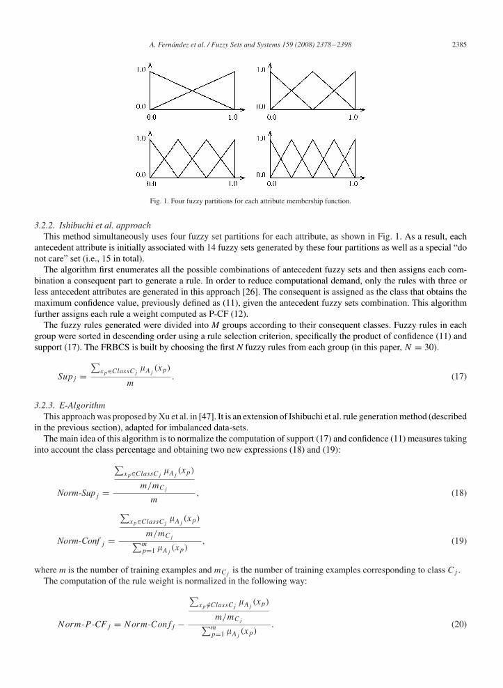
Fig. 1. Four fuzzy partitions for each attribute membership function.
3.2.2. Ishibuchi et al. approachThis method simultaneously uses four fuzzy set partitions for each attribute, as shown in Fig. 1. As a result, each
antecedent attribute is initially associated with 14 fuzzy sets generated by these four partitions as well as a special “donot care” set (i.e., 15 in total).
The algorithm first enumerates all the possible combinations of antecedent fuzzy sets and then assigns each com-bination a consequent part to generate a rule. In order to reduce computational demand, only the rules with three orless antecedent attributes are generated in this approach [26]. The consequent is assigned as the class that obtains themaximum confidence value, previously defined as (11), given the antecedent fuzzy sets combination. This algorithmfurther assigns each rule a weight computed as P-CF (12).
The fuzzy rules generated were divided into M groups according to their consequent classes. Fuzzy rules in eachgroup were sorted in descending order using a rule selection criterion, specifically the product of confidence (11) andsupport (17). The FRBCS is built by choosing the first N fuzzy rules from each group (in this paper, N = 30).
Supj =∑
xp∈ClassCj�Aj
(xp)
m. (17)
3.2.3. E-AlgorithmThis approach was proposed by Xu et al. in [47]. It is an extension of Ishibuchi et al. rule generation method (described
in the previous section), adapted for imbalanced data-sets.The main idea of this algorithm is to normalize the computation of support (17) and confidence (11) measures taking
into account the class percentage and obtaining two new expressions (18) and (19):
Norm-Supj =
∑xp∈ClassCj
�Aj(xp)
m/mCj
m, (18)
Norm-Conf j =
∑xp∈ClassCj
�Aj(xp)
m/mCj∑mp=1 �Aj
(xp), (19)
where m is the number of training examples and mCjis the number of training examples corresponding to class Cj .
The computation of the rule weight is normalized in the following way:
Norm-P -CFj = Norm-Confj −
∑xp /∈ClassCj
�Aj(xp)
m/mCj∑mp=1 �Aj
(xp). (20)
2386 A. Fernández et al. / Fuzzy Sets and Systems 159 (2008) 2378–2398
As in Ishibuchi et al. approach, using the product of the normalized support and confidence as the measure, a user-defined number of rules for each class N, is chosen from the initial rule set (also in this case, N = 30). These rules formthe fuzzy classification RB extracted from the data and are responsible for making decisions in classification tasks.
4. Analysis of FRBCS behaviour: cooperation with preprocessing techniques and study of the components
Our study is oriented towards analyzing the synergy between FRBCSs and preprocessing techniques and to compareand find the best-performing configurations for FRBCSs in the framework of imbalanced data-sets.
In this study we have considered 33 data-sets from UCI with different IR: from low imbalance to highly imbalanceddata-sets. Table 2 summarizes the data employed in this study and shows, for each data-set, the number of examples(#Ex.), number of attributes (#Atts.), class name of each class (minority and majority), class attribute distribution andIR. This table is ordered according to the IR, from low to high imbalance.
In order to develop our study we use a five fold cross validation approach, that is, five partitions for training andtest sets, 80% for training and 20% for testing, where the five test data-sets form the whole set. For each data-set weconsider the average results of the five partitions.
Table 2Data-sets summary descriptions
Data-set #Ex. #Atts. Class (min., maj.) %Class (min., maj.) IR
Data-sets with low imbalance (1.5–3 IR)Glass2 214 9 (build-window-non_float-proc, remainder) (35.51, 64.49) 1.82EcoliCP-IM 220 7 (im, cp) (35.00, 65.00) 1.86Wisconsin 683 9 (malignant, benign) (35.00, 65.00) 1.86Pima 768 8 (tested-positive, tested-negative) (34.84, 66.16) 1.90Iris1 150 4 (Iris-Setosa, remainder) (33.33, 66.67) 2.00Glass1 214 9 (build-window-float-proc, remainder) (32.71, 67.29) 2.06Yeast2 1484 8 (NUC, remainder) (28.91, 71.09) 2.46Vehicle2 846 18 (Saab, remainder) (28.37, 71.63) 2.52Vehicle3 846 18 (bus, remainder) (28.37, 71.63) 2.52Vehicle4 846 18 (Opel, remainder) (28.37, 71.63) 2.52Haberman 306 3 (Die, Survive) (27.42, 73.58) 2.68
Data-sets with medium imbalance (3–9 IR)GlassNW 214 9 (non-window glass, remainder) (23.83, 76.17) 3.19Vehicle1 846 18 (van, remainder) (23.64, 76.36) 3.23Ecoli2 336 7 (im, remainder) (22.92, 77.08) 3.36New-thyroid3 215 5 (hypo, remainder) (16.89, 83.11) 4.92New-thyroid2 215 5 (hyper, remainder) (16.28, 83.72) 5.14Ecoli3 336 7 (pp, remainder) (15.48, 84.52) 5.46Segment1 2308 19 (brickface, remainder) (14.26, 85.74) 6.01Glass7 214 9 (headlamps, remainder) (13.55, 86.45) 6.38Yeast4 1484 8 (ME3, remainder) (10.98, 89.02) 8.11Ecoli4 336 7 (iMU, remainder) (10.88, 89.12) 8.19Page-blocks 5472 10 (remainder, text) (10.23, 89.77) 8.77
Data-sets with high imbalance (higher than 9 IR)Vowel0 988 13 (hid, remainder) (9.01, 90.99) 10.10Glass3 214 9 (Ve-win-float-proc, remainder) (8.78, 91.22) 10.39Ecoli5 336 7 (om, remainder) (6.74, 93.26) 13.84Glass5 214 9 (containers, remainder) (6.07, 93.93) 15.47Abalone9-18 731 8 (18, 9) (5.65, 94.25) 16.68Glass6 214 9 (tableware, remainder) (4.20, 95.80) 22.81YeastCYT-POX 482 8 (POX, CYT) (4.15, 95.85) 23.10Yeast5 1484 8 (ME2, remainder) (3.43, 96.57) 28.41Yeast6 1484 8 (ME1, remainder) (2.96, 97.04) 32.78Yeast7 1484 8 (EXC, remainder) (2.49, 97.51) 39.16Abalone19 4174 8 (19, remainder) (0.77, 99.23) 128.87

A. Fernández et al. / Fuzzy Sets and Systems 159 (2008) 2378–2398 2387
Table 3Average results for FRBCSs with the different preprocessing mechanisms
Balance method GMTr GMTst
None 75.81 ± 26.23 61.94 ± 28.52CNNRb 72.27 ± 20.27 61.54 ± 23.09Tomek links 79.83 ± 24.34 67.00 ± 26.25OSS 68.70 ± 20.41 59.81 ± 23.18CNN-Tomek links 57.10 ± 23.64 50.41 ± 22.95NCL 80.17 ± 23.63 67.70 ± 26.20Random under-sampling 84.71 ± 11.36 75.16 ± 15.46Random over-sampling 90.67 ± 9.69 78.36 ± 15.45SMOTE 90.24 ± 9.96 79.57 ± 14.74SMOTE-Tomek links 88.76 ± 11.27 79.03 ± 15.08SMOTE-ENN 88.79 ± 10.77 78.97 ± 15.08
Table 4Wilcoxon’s test for the preprocessing mechanisms
Comparison R+ R− Hypothesis for � = 0.1
SMOTE vs. None 545.5 15.5 Rejected for SMOTE
Statistical analysis needs to be performed in order to find significant differences among the results obtained by themethods studied. We consider the use of non-parametric tests, according to the recommendations made in [11], wherea set of simple, safe and robust non-parametric tests for statistical comparisons of classifiers is presented. For pair wisecomparison we will use Wilcoxon’s signed-ranks test [44,34], and for multiple comparison we will employ differentapproaches, including Friedman’s test [15,16], Iman and Davenport’s test [21] and Holm’s method [20]. In all caseswe will use 0.10 as level of confidence (�). A wider description of these tests is presented in the Appendix.
This study is divided into four parts: first we will analyse the use of preprocessing for imbalanced problems usingthe mechanisms shown in Section 2.3. Then we will select a representative preprocessing method to study the influenceof the granularity applied to the linguistic partitions. Next we will study the Mansoori rule weight system approaches.Finally, with a fixed number of labels per variable, we will analyse the effect of the different possibilities for conjunctionoperators, rule weights and FRMs introduced in Section 3.1.
4.1. Preprocessing approach
The first objective in this study is to determine the synergy between preprocessing mechanisms and FRBCSs.After a previous study we have selected as a good FRBCS model the use of the product T-norm as conjunction
operator, together with the P-CF approach for the rule weight and FRM of the winning rule. We will study this modelcarefully in the last part of this section, but it will help us to analyse the preprocessing mechanisms of instances.
In Table 3 we present the average results for the different preprocessing approaches with the 33 selected imbalanceddata-sets where the name “None” indicates that we do not apply a preprocessing method (we use the original trainingdata-set). The test best result is stressed in boldface.
Our results clearly show that in almost all cases preprocessing is necessary in order to improve the behaviour ofFRBCSs. Specifically we can see that the over-sampling and hybrid methods achieve better performance in practice.We have found a type of mechanism, the SMOTE preprocessing family, that is very good as a preprocessing technique,in both the basic and hybrid approaches.
In Table 4 we show Wilcoxon’s test in order to compare the results using the SMOTE preprocessing mechanism withthe results using the original data-sets, where R+ is the sum of the ranks corresponding to the SMOTE approach andR− is the sum of the ranks corresponding to “no preprocessing” (original data-sets). The critical value associated withNds = 33 and p = 0.1, which can be found in the T Wilcoxon distribution (see [48, Table B.12]), is equal to 187.
It is statistically proved that the performance of the FRBCS is increased when using SMOTE rather than the originaldata-set, because the null hypothesis associated to Wilcoxon’s signed-ranks test is rejected when comparing both

2388 A. Fernández et al. / Fuzzy Sets and Systems 159 (2008) 2378–2398
Table 5Average results for FRBCSs varying the number of fuzzy labels
Number of labels GMTr GMTst
5 90.24 ± 9.96 79.57 ± 14.747 93.26 ± 7.64 73.54 ± 17.55
SMOTE method is used as preprocessing mechanism.
Table 6Wilcoxon’s test for the granularity of the fuzzy partitions
Comparison R+ R− Hypothesis for � = 0.1
5 Labels vs. 7 labels 505 56 Rejected for 5 labels
average results, due to the fact that the minimum ranking T (R− in this case) is lower than the critical value definedabove.
For the remainder of our experiments we will use the SMOTE preprocessing mechanism as representative of theover-sampling methods.
4.2. Analysis of the granularity of the fuzzy partitions
We focus now on the granularity of the fuzzy labels, determining the behaviour of the FRBCS when modifyingthe number of fuzzy subspaces per variable. Specifically, we will analyse the performance when using 5 and 7 labelsrespectively, as these are the two granularity levels most commonly employed in the specialized literature.
As in the preprocessing study, we will use the same pre-selected configuration of FRBCS, with product T-norm forthe conjunction operator, P-CF for the rule weight and the winning rule as FRM.
In Table 5 we show the average results for the 33 data-sets, using SMOTE as the preprocessing mechanism in boththe five and seven fuzzy partitions per variable.
In Table 5 it is empirically shown that a high number of labels produces over-fitting, that is, the test results aresignificantly worse than the training ones when we use 7 labels per variable.
Wilcoxon’s signed-ranks test, shown in Table 6, where R+ is the sum of the ranks corresponding to the FRBCSresults with 5 labels and R− is the sum of the ranks corresponding to the FRBCS results with 7 labels, confirms ourconclusion because clearly the critical value (187 for Nds = 33 and � = 0.1) is higher than the minimum ranking T(R− in this case).
For this reason, we will only employ 5 labels per variable in the remainder of this section.
4.3. Analysis of the Mansoori rule weight system approaches
In this section we will compare the two approaches of the Mansoori rule weight system [30] presented in Section 3.1,with RW = 1 and with RW = P-CF. In the case of the conjunction operator and the FRM, we will use the productT-norm and the winning rule, respectively, because it is the original configuration that the authors use in [30].
We will employ the SMOTE preprocessing method, as suggested by the results of Section 4.1, and 5 labels pervariable in the fuzzy partitions, because it has been shown in Section 4.2 that this achieves a better performance. InTable 7 we show the average results for the 33 data-sets in each case.
In Table 7 it is shown that the performance achieved with the basic mansoori rule weight system (RW = 1) is muchworse than when using this approach with the P-CF, both in training and test partitions.
Wilcoxon’s signed-ranks test, shown in Table 8, where R+ is the sum of the ranks corresponding to the results forthe Mansoori rule weight system with RW = 1 and R− is the sum of the ranks corresponding to the results for theMansoori rule weight system with RW = P-CF, confirms our conclusion because the critical value (187 for Nds = 33and � = 0.1) is higher than the minimum ranking T (R− in this case).
In accordance with these results, we will employ “RW = P-CF” for the Mansoori rule weight system.

A. Fernández et al. / Fuzzy Sets and Systems 159 (2008) 2378–2398 2389
Table 7Average results for FRBCSs using the Mansoori rule weight system
Rule weight GMTr GMTst
None (RW = 1) 79.02 ± 18.14 63.74 ± 22.48P-CF 90.58 ± 10.83 78.08 ± 17.00
SMOTE method is used as preprocessing mechanism.
Table 8Wilcoxon’s test for the Mansoori rule weight system comparison
Comparison R+ R− Hypothesis for � = 0.1
“RW = 1” vs. “P-CF” 18 543 Rejected for P-CF
Table 9Comparison of the average results for FRBCSs with different T-norms, rule weights and FRMs
Weight Conjunction operator Winning rule GMTr Winning rule GMTst Additive comb. GMTr Additive comb. GMTst
CF Minimum 89.46 ± 10.34 77.90 ± 15.49 88.20 ± 10.76 76.62 ± 17.87CF Product 90.83 ± 9.68 78.90 ± 14.87 90.77 ± 9.75 78.32 ± 17.00P-CF Minimum 90.02 ± 9.76 78.71 ± 15.15 89.22 ± 9.63 77.82 ± 15.37P-CF Product 90.24 ± 9.96 79.57 ± 14.74 90.80 ± 9.72 78.96 ± 15.75M-CF Minimum 88.75 ± 10.99 76.63 ± 17.57 83.91 ± 15.40 73.59 ± 17.46M-CF Product 90.58 ± 10.83 78.08 ± 17.00 85.03 ± 16.29 72.75 ± 18.98
Total – 89.98 ± 10.16 78.30 ± 15.67 87.99 ± 12.39 76.34 ± 17.06
SMOTE method is used as preprocessing mechanism.
4.4. Conjunction operators, FRM and rule weights
We will now study the effect of the conjunction operators (minimum and product T-norms) rule weights and FRMs,fixing SMOTE as the preprocessing mechanism and the number of fuzzy subspaces as 5 labels per variable.
Table 9 shows the experimental results obtained with the different configurations for FRBCSs, and is divided intotwo parts using as FRM the winning rule and additive combination, respectively. The following information is shownby columns:
• The first column “Weight” is the rule weight used in the FRBCS. Following the same notation as in Section 3.1CF stands for the certainty factor, P-CF stands for the penalized certainty factor and M-CF stands for the Mansooriweighting system.
• Inside the column “Conjunction operator” we note whether the results correspond to the minimum or product T-norm.• Finally, in the last four columns the average results for the geometric mean of the true rates in training (GMTr) and
test (GMTst) are shown for each FRM approach. We focus our analysis on the generalization capacity via the testpartition. In this manner, the best test result is stressed in boldface.
In order to compare the results, we will use a multiple comparison test to find the best configuration in each case,that is, for the FRM of the winning rule and additive combination separately. In Table 10, the results of applying theFriedman and Iman–Davenport tests are shown in order to see if there are differences in the results. We employ the�2-distribution with 5 degrees of freedom and the F-distribution with 5 and 160 degrees of freedom for Nds = 33. Weemphasize in bold the highest value between the two values that are being compared, and as the smallest in both casescorresponds to the value given by the statistic, it informs us of the rejection of the null hypothesis and, in this manner,Friedman test and Iman–Davenport tests tell us of the existence of significant differences among the observed resultsin all data-sets.
According to these results, a post hoc statistical analysis is needed. Tables 11 and 12 show the rankings (computedusing Friedman’s test) of the six different configurations for the FRBCS considered.

2390 A. Fernández et al. / Fuzzy Sets and Systems 159 (2008) 2378–2398
Table 10Results of Friedman and Iman–Davenport’s tests for comparing performance when using different configurations in the FRBCS for FRM of thewinning rule and additive combination
FRM Friedman Value in �2 Iman–Davenport Value in FF
Winning rule 19.822 9.2364 4.369 1.8836Additive comb. 14.524 9.2364 3.089 1.8836
Table 11Rankings obtained through Friedman’s test for FRBCS configuration. FRM of the winning rule
T-norm + rule weight Ranking
Product + P-CF 2.7727Product + CF 3.0454Product + M-CF 3.2273Minimum + P-CF 3.4091Minimum + CF 4.0606Minimum + M-CF 4.4848
Table 12Rankings obtained through Friedman’s test for FRBCS configuration. FRM of additive combination
T-norm + rule weight Ranking
Product + CF 2.8485Product + P-CF 2.8939Product + M-CF 3.5606Minimum + CF 3.5909Minimum + P-CF 3.8030Minimum + M-CF 4.3030
Table 13Holm’s table for the configuration of the FRBCS. FRM of the winning rule (FRBCS with product T-norm and P-CF for the rule weight is the controlmethod)
i Algorithm z p �/i Hypothesis
5 Minimum + M-CF 3.71742 0.00020 0.0125 R for Product + P-CF4 Minimum + CF 2.79629 0.00517 0.0167 R for Product + P-CF3 Minimum + P-CF 1.38170 0.16706 0.025 A2 Product + M-CF 0.98693 0.32368 0.05 A1 Product + CF 0.59216 0.55375 0.1 A
In the first case (Table 11) the best ranking is obtained by the FRBCS that uses product T-norm and P-CF for therule weight. In the second case (Table 12) the best ranking corresponds to the FRBCS that uses product T-norm andCF for the rule weight.
We now apply Holm’s test to compare the best ranking method in each case with the remaining methods. In order toshow the results of this test, we will present the tables associated with Holm’s procedure, in which all the computationsare shown. Table 13 presents the results for the FRM of the winning rule, while Table 14 shows the results for the FRMof additive combination.
In these tables the algorithms are ordered with respect to the z-value obtained. Thus, by using the normal distribution,we can obtain the corresponding p-value associated with each comparison and this can be compared with the associated�/i in the same row of the table to show whether the associated hypothesis of equal behaviour is rejected in favour ofthe best ranking algorithm (marked with an R) or not (marked with an A).
The tests reject the hypothesis of equality of means for the two worst configurations compared with the remain-ing ones but they do not distinguish any difference among the rest of the configurations for FRBCSs with the best

A. Fernández et al. / Fuzzy Sets and Systems 159 (2008) 2378–2398 2391
Table 14Holm’s table for the configuration of the FRBCS. FRM of additive combination (FRBCS with product T-norm and CF for the rule weight is thecontrol method)
i Algorithm z p �/i Hypothesis
5 Minimum + M-CF 3.15817 0.00159 0.0125 R for product + CF4 Minimum + P-CF 2.07255 0.03821 0.0167 R for product + CF3 Minimum + CF 1.61198 0.10697 0.025 A2 Product + M-CF 1.54619 0.12206 0.05 A1 Product + P-CF 0.09869 0.92138 0.1 A
Table 15Wilcoxon’s test for the FRBCS configuration
Comparison R+ R− Hypothesis
WR vs. AC 286 275 Accepted
approach in each case. Nevertheless, we can extract some interesting conclusions from the ranking of the differentFRBCS approaches:
(1) Regarding the conjunction operator, we can conclude that very good performance is achieved when using theproduct T-norm rather than the minimum T-norm, independently of the rule weight and FRM.
(2) For the rule weight we may emphasize as good configurations the P-CF in the case of the FRM of the winning ruleand the CF in the case of the FRM with additive combination. They have a higher ranking, although statisticallythey are similar to the remaining configurations.
Finally we compare the two best approaches for the FRM of the winning rule and additive combination in orderto obtain the best global configuration for FRBCS in imbalanced data-sets. To do this, we will apply a Wilcoxon’ssigned-ranks test (shown in Table 15) to compare the FRBCS with product T-norm, P-CF for the rule weight and FRMof the winning rule vs. the FRBCS with product T-norm, CF for the rule weight and FRM of additive combination.
We can see that both approaches are statistically equal, because the minimum ranking (the one associated to theadditive combination) is higher than the critical value of Wilcoxon distribution (again 187). Since the FRM of thewinning rule obtains a better ranking than the additive combination, we select as a good model the one based inFRM of the winning rule, with product T-norm and P-CF for the rule weight. Observing Table 9, we can see that thisconfiguration obtains the best performance in the average geometric mean of the true ratios (79.57).
5. Analysis of FRBCS behaviour according to the degree of imbalance
In the last part of our study we present a statistical analysis where we compare the selected model for the linguisticFRBCS based on the Chi et al. rule generation [6] (obtained in the previous section) with an FRBCS based on theIshibuchi et al. rule generation [24–26] and with the E-Algorithm [47], an ad hoc procedure for imbalanced data-sets.We also include C4.5 in this comparison, because it is an algorithm of reference in this area [2].
Until now we have treated the problem of imbalanced data-sets without regard the percentage of positive and negativeinstances. However, in this section we use the IR to distinguish between three classes of imbalanced data-sets: data-setswith a low imbalance when the instances of the positive class are between 25% and 40% of the total instances (IRbetween 1.5 and 3), data-sets with a medium imbalance when the number of the positive instances is between 10% and25% of the total instances (IR between 3 and 9), and data-sets with a high imbalance where there are no more than10% of positive instances in the whole data-set compared to the negative ones (IR higher than 9).
Following the scheme defined above, this study is shown in Tables 16, 20 and 24, each one focussing on low,medium and high imbalance, respectively. These tables show the results for FRBCSs obtained with the Chi et al. andthe Ishibuchi et al. rule generation methods using product T-norm, P-CF for the rule weight and FRM of the winningrule in all cases. We also show the results for the E-Algorithm with the same configuration as the FRBCSs approaches,and the results for the C4.5 decision tree.

2392 A. Fernández et al. / Fuzzy Sets and Systems 159 (2008) 2378–2398
Table 16Global comparison of FRBCSs (Chi et al. and Ishibuchi et al.), E-Algorithm and C4.5. Data-sets with low imbalance
Data-set FRBCS-Chi SMOTE pre. FRBCS-Ish SMOTE pre. E-Algorithm no preprocessing C4.5 SMOTE pre.
GMTr GMTst GMTr GMTst GMTr GMTst GMTr GMTst
EcoliCP-IM 98.19 95.56 97.00 96.70 95.16 95.25 99.26 97.95Haberman 70.86 60.40 64.36 62.65 8.47 4.94 74.00 61.32Iris1 100.00 98.97 100.00 100.00 100.00 100.00 100.00 98.97Pima 85.53 66.78 71.31 71.10 55.86 55.01 83.88 71.26Vehicle3 96.36 87.19 66.28 67.82 46.24 43.83 98.95 94.85Wisconsin 99.72 43.58 96.17 95.78 96.04 96.01 98.31 95.44Yeast2 72.75 69.66 51.83 51.41 0.00 0.00 80.34 70.86Glass1 74.44 63.69 72.22 69.39 0.00 0.00 94.23 78.14Glass2 77.30 64.91 65.33 59.29 10.24 0.00 89.74 75.11Vehicle2 91.18 71.88 64.83 64.89 5.93 3.09 95.50 69.28Vehicle4 90.22 63.13 63.21 63.12 0.00 0.00 94.88 74.34
Average 86.96 71.43 73.87 72.92 37.99 36.19 91.74 80.68Std. dev 11.35 16.38 16.21 16.67 42.27 43.43 8.72 13.49
Table 17Rankings obtained through Friedman’s test for FRBCSs (Chi et al. and Ishibuchi et al.), E-Algorithm and C4.5 in data-sets with low imbalance
Method Ranking
C4.5 1.5909FRBCS-Ishibuchi 2.3182FRBCS-Chi 2.5909E-Algorithm 3.5
Table 18Holm’s table for FRBCSs (Chi et al. and Ishibuchi et al.), E-Algorithm and C4.5 in data-sets with low imbalance. C4.5 is the control method
i Algorithm z p �/i Hypothesis
3 E-Algorithm 3.46804 0.00052 0.03333 Rejected for C4.52 FRBCS-Chi 1.81659 0.06928 0.05 Accepted1 FRBCS-Ishibuchi 1.32116 0.18645 0.1 Accepted
We employ the SMOTE preprocessing method for the FRBCSs (Chi et al. and Ishibuchi et al.) and for C4.5. TheE-Algorithm is always applied without preprocessing.
We also apply Friedman and Iman–Davenport tests in order to detect the possible differences among the FRBCSsapproaches, the E-Algorithm and C4.5 in each case. We employ the �2-distribution with 2 degrees of freedom and theF-distribution with 2 and 20 degrees of freedom for Nds = 11. If significant differences are found with these tests,Holm’s post hoc test will be applied in order to find the best configuration.
5.1. Data-sets with low imbalance
This study is shown in Table 16. The p-values computed using Friedman’s test (0.006342) and Iman–Davenport’s test(0.00258) are lower than our level of confidence � = 0.1, which implies that there are statistical differences among theresults. In this manner, Table 17 shows the rankings (computed using Friedman’s test) of the four algorithms considered.
In this kind of data-sets C4.5 is better in ranking, but Holm’s Test (Table 18) only rejects the null hypothesis in thecase of the E-Algorithm. A Wilcoxon’s test (Table 19) is needed in order to confirm that C4.5 is statistically better thanthe FRBCS obtained with the Ishibuchi et al. approach, which is the second in ranking.

A. Fernández et al. / Fuzzy Sets and Systems 159 (2008) 2378–2398 2393
Table 19Wilcoxon’s test in data-sets with low imbalance. R+ corresponds to the FRBCS (Ishibuchi et al. approach) and R− to C4.5
Comparison R+ R− Hypothesis p-Value
FRBCS-Ish vs. C4.5 10 56 Rejected for C4.5 0.041
Table 20Global comparison of FRBCSs (Chi et al. and Ishibuchi et al.), E-Algorithm and C4.5. Data-sets with medium imbalance
Data-set FRBCS-Chi SMOTE pre. FRBCS-Ish SMOTE pre. E-Algorithm no preprocessing C4.5 SMOTE pre.
GMTr GMTst GMTr GMTst GMTr GMTst GMTr GMTst
Ecoli2 93.78 86.05 85.45 85.71 75.34 77.81 96.28 76.10GlassNW 98.48 85.94 85.68 88.56 82.08 82.09 99.07 90.13New-thyroid2 99.58 95.38 90.97 89.02 88.92 88.52 99.21 97.98New-thyroid3 99.58 96.34 94.34 94.21 88.94 88.57 99.57 96.51Page-blocks 88.64 87.25 32.41 32.16 64.65 64.51 98.46 94.84Segment 98.19 95.88 42.61 42.47 95.64 95.33 99.85 99.26Vehicle1 96.26 84.93 76.54 75.94 44.68 39.07 98.97 91.10Ecoli3 92.90 87.64 87.23 87.00 71.98 70.35 95.11 91.60Yeast4 92.01 89.33 79.97 77.06 82.09 81.99 95.64 88.50Glass7 94.75 91.61 85.78 85.39 80.21 78.54 98.14 88.77Ecoli4 98.06 78.13 86.42 86.27 90.84 90.23 99.59 83.00
Average 95.66 88.95 77.04 76.71 78.67 77.91 98.17 90.71Std. dev 3.55 5.54 20.23 20.27 14.42 15.69 1.70 6.78
Table 21Rankings obtained through Friedman’s test for FRBCSs (Chi et al. and Ishibuchi et al.), E-Algorithm and C4.5 in data-sets with medium imbalance
Method Ranking
C4.5 1.6364FRBCS-Chi 2.0FRBCS-Ishibuchi 3.0E-Algorithm 3.3636
Because of the fact that we are dealing with data-sets with a low imbalance, the low classification rates for the FRBCSscould be due to the characteristics of the data-sets, not only to the imbalance and overlapping between classes.
In the case of the E-Algorithm, some results in training and test have a 0 value. This is due to the fact that a subset ofrules is selected from the total by means of the product between confidence and support (normalized values). For thepositive class, rules with high confidence have low support, so these rules obtain a low score in the selection process.The rules selected for the positive class are never fired because they have less weight than the rules of the negative class(whose support is higher), and all instances of the positive class are classified as negative, resulting in a 0 value for thegeometric mean of the true rates.
5.2. Data-sets with medium imbalance
This study is shown in Table 20. Also in this case the Friedman and Iman–Davenport tests detect significant differencesamong the results of the algorithms, with an error value for Friedman’s test of 0.00433238 and 0.0014477 for Iman–Davenport’s test.
Observing a smaller difference between our selected model for the FRBCS (Chi et al.) and C4.5, we may concludethat in this case the FRBCS improves its behaviour. We can see the similar ranking value for the FRBCS (Chi et al.)and C4.5 obtained by Friedman’s test in Table 21. Even Holm’s (Table 22) and Wilcoxon’s tests (Table 23) accept thenull hypothesis when comparing both algorithms, which helps to confirm our conclusion.
2394 A. Fernández et al. / Fuzzy Sets and Systems 159 (2008) 2378–2398
Table 22Holm’s table for FRBCSs (Chi et al. and Ishibuchi et al.), E-Algorithm and in data-sets with medium imbalance. C4.5 is the control method
i Algorithm z p �/i Hypothesis
3 E-Algorithm 3.13775 0.00170 0.03333 Rejected for C4.52 FRBCS-Ishibuchi 2.47717 0.01324 0.05 Rejected for C4.51 FRBCS-Chi 0.66058 0.50888 0.1 Accepted
Table 23Wilcoxon’s test in data-sets with medium imbalance. R+ corresponds to the FRBCS (Chi et al. approach) and R− to C4.5
Comparison R+ R− Hypothesis p-value
FRBCS-Chi vs. C4.5 17 49 Accepted 0.155
Table 24Global comparison of FRBCSs (Chi et al. and Ishibuchi et al.), E-Algorithm and C4.5. Data-sets with high imbalance
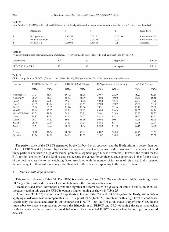
Data-set FRBCS-Chi SMOTE pre. FRBCS-Ish SMOTE pre. E-Algorithm no preprocessing C4.5 SMOTE pre.
GMTr GMTst GMTr GMTst GMTr GMTst GMTr GMTst
Abalone9-18 71.07 66.47 66.42 65.78 39.67 32.29 95.20 53.19Abalone19 75.99 66.71 66.93 66.09 0.00 0.00 84.31 15.58Ecoli5 98.12 92.11 89.21 86.92 92.80 92.43 97.67 81.28Glass3 71.39 49.24 45.25 43.55 27.03 9.87 95.68 33.86Yeast5 87.94 83.07 75.80 71.36 38.31 32.16 90.76 65.00Vowel0 99.64 97.87 89.99 89.03 89.84 89.63 99.67 94.74YeastCYT-POX 82.35 78.76 74.01 72.83 74.01 72.83 90.93 78.23Glass5 98.87 81.75 87.03 78.27 84.82 83.38 98.42 83.71Glass6 98.77 64.33 89.88 89.96 80.60 50.61 99.76 86.70Yeast5 95.40 93.64 94.93 94.94 88.66 88.17 97.75 92.04Yeast7 89.57 87.73 88.48 88.42 53.82 51.72 92.15 80.38
Average 88.10 78.34 78.90 77.01 60.87 54.83 94.75 69.52Std. dev 11.26 14.99 14.93 15.09 31.02 33.09 4.77 25.38
The performance of the FRBCS generated by the Ishibuchi et al. approach and the E-Algorithm is poorer than ourselected FRBCS model (obtained by the Chi et al. approach) and C4.5, because of the restriction in the number of validfuzzy partitions per rule in high dimensional problems (segment, page-blocks or vehicle). However, the results for theE-Algorithm are better for this kind of data-set because the values for confidence and support are higher for the rulesof the positive class due to the weighting factor associated with the number of instances of this class. In this mannerthe rule weight of these rules is now greater than that of the rules corresponding to the negative class.
5.3. Data-sets with high imbalance
This study is shown in Table 24. The FRBCSs clearly outperform C4.5. We can observe a high overfitting in theC4.5 algorithm, with a difference of 25 points between the training and test results.
Friedman’s and Iman–Davenport’s tests find significant differences with a p-value of 0.01335 and 0.0074888, re-spectively, and in this case the FRBCSs obtain a higher ranking as shown in Table 25.
Holm’s test (Table 26) rejects the null hypothesis in favour of the Chi et al. FRBCS against the E-Algorithm. Whenapplying a Wilcoxon test to compare this FRBCS against C4.5 (Table 27), we obtain with a high level of confidence(specifically the associated error in this comparison is 0.075) that the Chi et al. model outperforms C4.5. In thesame table we make a comparison between the Ishibuchi et al. FRBCS and C4.5, obtaining the same conclusion.In this manner we have shown the good behaviour of our selected FRBCS model when facing high imbalanceddata-sets.
A. Fernández et al. / Fuzzy Sets and Systems 159 (2008) 2378–2398 2395
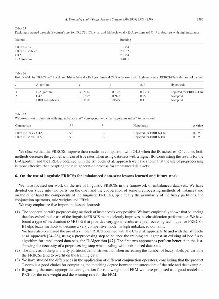
Table 25Rankings obtained through Friedman’s test for FRBCSs (Chi et al. and Ishibuchi et al.), E-Algorithm and C4.5 in data-sets with high imbalance
Method Ranking
FRBCS-Chi 1.6364FRBCS-Ishibuchi 2.3182C4.5 2.6364E-Algorithm 3.4091
Table 26Holm’s table for FRBCSs (Chi et al. and Ishibuchi et al.), E-Algorithm and C4.5 in data-sets with high imbalance. FRBCS-Chi is the control method
i Algorithm z p �/i Hypothesis
3 E-Algorithm 3.22032 0.00128 0.03333 Rejected for FRBCS-Chi2 C4.5 1.81659 0.06928 0.05 Accepted1 FRBCS-Ishibuchi 1.23858 0.21549 0.1 Accepted
Table 27Wilcoxon’s test in data-sets with high imbalance. R+ corresponds to the first algorithm and R− to the second
Comparison R+ R− Hypothesis p-value
FRBCS-Chi vs. C4.5 53 13 Rejected for FRBCS-Chi 0.075FRBCS-Ish vs. C4.5 53 13 Rejected for FRBCS-Ish 0.075
We observe that the FRBCSs improve their results in comparison with C4.5 when the IR increases. Of course, bothmethods decrease the geometric mean of true rates when using data-sets with a higher IR. Contrasting the results for theE-Algorithm and the FRBCS obtained with the Ishibuchi et al. approach we have shown that the use of preprocessingis more effective than adapting the rule generation process for imbalanced data-sets.
6. On the use of linguistic FRBCSs for imbalanced data-sets: lessons learned and future work
We have focused our work on the use of linguistic FRBCSs in the framework of imbalanced data-sets. We havedivided our study into two parts: on the one hand the cooperation of some preprocessing methods of instances andon the other hand the components of the linguistic FRBCSs, specifically the granularity of the fuzzy partitions, theconjunction operators, rule weights and FRMs.
We may emphasize five important lessons learned:
(1) The cooperation with preprocessing methods of instances is very positive. We have empirically shown that balancingthe classes before the use of the linguistic FRBCS method clearly improves the classification performance. We havefound a type of mechanism (SMOTE) that provides very good results as a preprocessing technique for FRBCSs.It helps fuzzy methods to become a very competitive model in high imbalanced domains.We have also compared the use of a simple FRBCS obtained with the Chi et al. approach [6] and with the Ishibuchiet al. approach [24–26], using a preprocessing step to balance the training set, against an existing ad hoc fuzzyalgorithm for imbalanced data-sets, the E-Algorithm [47]. The first two approaches perform better than the last,showing the necessity of a preprocessing step when dealing with imbalanced data-sets.
(2) The analysis of the granularity partitions demonstrates that when increasing the number of fuzzy labels per variablethe FRBCSs tend to overfit on the training data.
(3) We have studied the differences in the application of different conjunction operators, concluding that the productT-norm is a good choice for computing the matching degree between the antecedent of the rule and the example.
(4) Regarding the most appropriate configuration for rule weight and FRM we have proposed as a good model theP-CF for the rule weight and the winning rule for the FRM.

2396 A. Fernández et al. / Fuzzy Sets and Systems 159 (2008) 2378–2398
(5) Comparing the performance of FRBCSs in contrast with the well-known algorithm C4.5, the latter obtains goodresults when the IR is low or medium, but when this ratio increases then the FRBCSs are more robust to the classimbalance problem and in data-sets with high imbalance our approach outperforms C4.5.
As future work our intention is to develop effective learning approaches for fuzzy rules extraction that allow us tolearn good RBs for different imbalance degrees. Specifically, we are currently studying two approaches: a HierarchicalSystem of Linguistic Rules Learning Methodology [9] and the generation of the Knowledge Base by the GeneticLearning of the Data Base [8].
7. Concluding remarks
In this work we have considered the problem of imbalanced data-sets in classification using linguistic FRBCSs. Wehave studied the cooperation of some preprocessing methods of instances and we have analysed the configuration ofthe FRBCS, studying the granularity of the fuzzy partitions, the conjunction operators, the rule weights and the FRMs.
Our results have shown the necessity of using preprocessing methods of instances to improve the balance betweenclasses before the use of the FRBCS method. Furthermore, when contrasting the use of a linguistic FRBCS speciallybuilt for imbalanced data-sets (the E-Algorithm) with the use of preprocessing techniques, the latter have shown a greatadvantage in the classification task of imbalanced data-sets with linguistic FRBCSs.
We have suggested as good components the following ones: the product T-norm as conjunction operator and theP-CF as rule weight. Regarding the FRM there are few differences, and we have chosen the winning rule approach;nevertheless, in the design of a learning method both approaches must be analysed.
Finally, we have found that the linguistic FRBCSs perform well against the C4.5 decision tree in the framework ofhighly imbalanced data-sets.
Appendix A. On the use of non-parametric tests based on rankings
A non-parametric test is that which uses nominal data or ordinal data or data represented in an ordinal way of ranking.This does not imply that only them must be used for these types of data. It could be very interesting to transform thedata from real values contained within an interval to ranking based data, in the way as a non-parametric test can beapplied over typical data of parametric test when they do not fulfill the needed conditions imposed by the use ofthe test.
In the following, we explain the basic functionality of each non-parametric test used in this study together with theaim pursued by its use:
• Friedman’s test: It is a non-parametric equivalent of the test of repeated-measures ANOVA. It computes the rankingof the observed results for algorithm (rj for the algorithm j with k algorithms) for each data-set, assigning to thebest of them the ranking 1, and to the worst the ranking k. Under the null hypothesis, formed from supposing theresults of the algorithms are equivalents and, therefore, their rankings are also similar, Friedman’s statistic
�2F = 12Nds
k(k + 1)
⎡⎣∑
j
R2j − k(k + 1)2
4
⎤⎦ , (A.1)
is distributed according to �2F with k−1 degrees of freedom, being Rj = 1
Nds
∑i r
ji , and Nds the number of data-sets.
The critical values for Friedman’s statistic coincide with the established in the �2 distribution when Nds > 10 andk > 5. In a contrary case, the exact values can be seen in [34,48].
• Iman and Davenport’s test [21]: It is a metric derived from Friedman’s statistic given that this last metric producesa conservative undesirable effect. The statistic is
FF = (Nds − 1)�2F
Nds(k − 1) − �2F
, (A.2)
and it is distributed according to a F-distribution with k − 1 and (k − 1)(Nds − 1) degrees of freedom.

A. Fernández et al. / Fuzzy Sets and Systems 159 (2008) 2378–2398 2397
• Holm’s method [20]: This test sequentially checks the hypothesis ordered according to their significance. We willdenote the p-values ordered by p1, p2, . . . , in the way that p1 �p2 � · · · �pk−1. Holm’s method compares each pi
with �/(k − i) starting from the most significant p-value. If p1 is below than �/(k −1), the corresponding hypothesisis rejected and it let us to compare p2 with �/(k − 2). If the second hypothesis is rejected, we continue with theprocess. As soon as a certain hypothesis cannot be rejected, all the remaining hypothesis are maintained as accepted.The statistic for comparing the i algorithm with the j algorithm is
z = (Ri − Rj )/
√k(k + 1)
6Nds. (A.3)
The value of z is used for finding the corresponding probability from the table of the normal distribution, whichis compared with the corresponding value of �.
• Wilcoxon’s signed-rank test: This is the analogous of the paired t-test in non-parametrical statistical procedures;therefore, it is a pair wise test that aims to detect significant differences between the behaviour of two algorithms.
Let di be the difference between the performance scores of the two classifiers on ith out of Nds data-sets. Thedifferences are ranked according to their absolute values; average ranks are assigned in case of ties. Let R+ be thesum of ranks for the data-sets on which the first algorithm outperformed the second, and R− the sum of ranks forthe opposite. Ranks of di = 0 are split evenly among the sums; if there is an odd number of them, one is ignored:
R+ =∑di>0
rank(di) + 1
2
∑di=0
rank(di), (A.4)
R− =∑di<0
rank(di) + 1
2
∑di=0
rank(di). (A.5)
Let T be the smallest of the sums, T = min(R+, R−). If T is less than or equal to the value of the distribution ofWilcoxon for Nds degrees of freedom [48, Table B.12], the null hypothesis of equality of means is rejected.
References
[1] R. Barandela, J. Sánchez, V. García, E. Rangel, Strategies for learning in class imbalance problems, Pattern Recognition 36 (3) (2003)849–851.
[2] G. Batista, R. Prati, M. Monard, A study of the behaviour of several methods for balancing machine learning training data, SIGKDD Explorations6 (1) (2004) 20–29.
[3] P. Campadelli, E. Casiraghi, G. Valentini, Support vector machines for candidate nodules classification, Lett. Neurocomputing 68 (2005)281–288.
[4] N. Chawla, K. Bowyer, L. Hall, W. Kegelmeyer, Smote: synthetic minority over-sampling technique, J. Artificial Intelligent Res. 16 (2002)321–357.
[5] N. Chawla, N. Japkowicz, A. Kolcz, Editorial: special issue on learning from imbalanced data sets, SIGKDD Explorations 6 (1) (2004) 1–6.[6] Z. Chi, H. Yan, T. Pham, Fuzzy algorithms with applications to image processing and pattern recognition, World Scientific, Singapore, 1996.[7] O. Cordón, M.J. del Jesus, F. Herrera, A proposal on reasoning methods in fuzzy rule-based classification systems, Internat. J. Approx. Reason.
20 (1) (1999) 21–45.[8] O. Cordón, F. Herrera, P. Villar, Generating the knowledge base of a fuzzy rule-based system by the genetic learning of the data base, IEEE
Trans. Fuzzy Systems 9 (4) (2001) 667–674.[9] O. Cordón, F. Herrera, I. Zwir, Linguistic modeling by hierarchical systems of linguistic rules, IEEE Trans. Fuzzy Systems 10 (1) (2002) 2–20.
[10] K. Crockett, Z. Bandar, J. O’Shea, On producing balanced fuzzy decision tree classifiers, in: IEEE Internat. Conf. on Fuzzy Systems, 2006,pp. 1756–1762.
[11] J. Demšar, Statistical comparisons of classifiers over multiple data sets, J. Mach. Learning Res. 7 (2006) 1–30.[12] O. Dunn, Multiple comparisons among means, J. Amer. Statist. Assoc. 56 (1961) 52–64.[13] A. Estabrooks, T. Jo, N. Japkowicz, A multiple resampling method for learning from imbalanced data sets, Comput. Intelligence 20 (1) (2004)
18–36.[14] T. Fawcett, F.J. Provost, Adaptive fraud detection, Data Mining Knowledge Discovery 1 (3) (1997) 291–316.[15] M. Friedman, The use of ranks to avoid the assumption of normality implicit in the analysis of variance, J. Amer. Statist. Assoc. 32 (1937)
675–701.[16] M. Friedman, A comparison of alternative tests of significance for the problem of m rankings, Ann. Math. Statist. 11 (1940) 86–92.[17] J.W. Grzymala-Busse, L.K. Goodwin, X. Zhang, Increasing sensitivity of preterm birth by changing rule strengths, Pattern Recognition Lett.
24 (6) (2003) 903–910.

2398 A. Fernández et al. / Fuzzy Sets and Systems 159 (2008) 2378–2398
[18] H. Guo, H.L. Viktor, Learning from imbalanced data sets with boosting and data generation: the databoost-im approach, SIGKDD Explorations6 (1) (2004) 30–39.
[19] P. Hart, The condensed nearest neighbor rule, IEEE Trans. Inform. Theory 14 (1968) 515–516.[20] S. Holm, A simple sequentially rejective multiple test procedure, Scand. J. Statist. 6 (1979) 65–70.[21] R. Iman, J. Davenport, Approximations of the critical region of the friedman statistic, Comm. Statist. Part A Theory Methods 9 (1980)
571–595.[22] H. Ishibuchi, T. Nakashima, Effect of rule weights in fuzzy rule-based classification systems, IEEE Trans. Fuzzy Systems 9 (4) (2001)
506–515.[23] H. Ishibuchi, T. Nakashima, M. Nii, Classification and Modeling with Linguistic Information Granules: Advanced Approaches to Linguistic
Data Mining, Springer, Berlin, 2004.[24] H. Ishibuchi, T. Yamamoto, Fuzzy rule selection by multi-objective genetic local search algorithms and rule evaluation measures in data mining,
Fuzzy Sets and Systems 141 (1) (2004) 59–88.[25] H. Ishibuchi, T. Yamamoto, Comparison of heuristic criteria for fuzzy rule selection in classification problems, Fuzzy Optim. Decision Making
3 (2) (2004) 119–139.[26] H. Ishibuchi, T. Yamamoto, Rule weight specification in fuzzy rule-based classification systems, IEEE Trans. Fuzzy Systems 13 (2005)
428–435.[27] N. Japkowicz, S. Stephen, The class imbalance problem: a systematic study, Intelligent Data Anal. 6 (5) (2002) 429–450.[28] M. Kubat, R. Holte, S. Matwin, Machine learning for the detection of oil spills in satellite radar images, Mach. Learning 30 (2–3) (1998)
195–215.[29] M. Kubat, S. Matwin, Addressing the curse of imbalanced training sets: one-sided selection, in: Internat. Conf. Machine Learning, 1997,
pp. 179–186.[30] E. Mansoori, M. Zolghadri, S. Katebi, A weighting function for improving fuzzy classification systems performance, Fuzzy Sets and Systems
158 (5) (2007) 583–591.[31] A. Orriols-Puig, E. Bernadó-Mansilla, K. Sastry, D.E. Goldberg, Substructural surrogates for learning decomposable classification problems:
implementation and first results, in: GECCO ’07: Proceedings of the 2007 GECCO Conference Companion on Genetic and EvolutionaryComputation, ACM Press, New York, NY, USA, 2007, pp. 2875–2882.
[32] F. Provost, T. Fawcett, Robust classification for imprecise environments, Mach. Learning 42 (3) (2001) 203–231.[33] B. Raskutti, A. Kowalczyk, Extreme rebalancing for SVMs: a case study, SIGKDD Explorations 6 (1) (2004) 60–69.[34] D. Sheskin, Handbook of Parametric and Nonparametric Statistical Procedures, Chapman & Hall, CRC, London, Boca Raton, 2003.[35] V. Soler, J. Cerquides, J. Sabria, J. Roig, M. Prim, Imbalanced datasets classification by fuzzy rule extraction and genetic algorithms, in: IEEE
Internat. Conf. Data Mining—Workshops, 2006, pp. 330–336.[36] I. Tomek, Two modifications of cnn, IEEE Trans. Systems Man Comm. 6 (1976) 769–772.[37] S. Visa, A. Ralescu, Learning imbalanced and overlapping classes using fuzzy sets, in: Internat. Conf. Machine Learning—Workshop on
Learning from Imbalanced Datasets II, 2003.[38] S. Visa, A. Ralescu, Fuzzy classifiers for imbalanced, complex classes of varying size, in: Information Processing and Management of Uncertainty
in Knowledge-Based Systems, 2004, pp. 393–400.[39] S. Visa, A. Ralescu, The effect of imbalanced data class distribution on fuzzy classifiers—experimental study, in: IEEE Internat. Conf. on Fuzzy
Systems, 2005, pp. 749–754.[40] L. Wang, J. Mendel, Generating fuzzy rules by learning from examples, IEEE Trans. Systems Man Cybernet. 25 (2) (1992) 353–361.[41] G. Weiss, Mining with rarity: a unifying framework, SIGKDD Explorations 6 (1) (2004) 7–19.[42] G. Weiss, H. Hirsh, A quantitative study of small disjuncts, in: National Conf. Artificial Intelligence, 2000, pp. 665–670.[43] G. Weiss, F. Provost, Learning when training data are costly: the effect of class distribution on tree induction, J. Artificial Intelligence Res. 19
(2003) 315–354.[44] F. Wilcoxon, Individual comparisons by ranking methods, Biometrics 1 (1945) 80–83.[45] D.R. Wilson, Asymptotic properties of nearest neighbor rules using edited data, IEEE Trans. Systems Man Comm. 2 (3) (1972) 408–421.[46] D.R. Wilson, T.R. Martinez, Reduction techniques for instance-based learning algorithms, Mach. Learning 38 (3) (2000) 257–286.[47] L. Xu, M. Chow, L. Taylor, Power distribution fault cause identification with imbalanced data using the data mining-based fuzzy classification
e-algorithm, IEEE Trans. Power Systems 22 (1) (2007) 164–171.[48] J. Zar, Biostatistical Analysis, Prentice-Hall, Upper Saddle River, NJ, 1999.[49] L. Zhuang, H. Dai, X. Hang, A novel field learning algorithm for dual imbalance text classification, in: International Conf. on Fuzzy Systems
and Knowledge Discovery, Lecture Notes on Artificial Intelligence, Vol. 3614, 2005, pp. 39–48.