A STUDY OF SHOCK ANALYSIS USING THE FINITE ELEMENT METHOD VERIFIED

WITH EULER-BERNOULLI BEAM THEORY; MECHANICAL EFFECTS DUE TO

PULSE WIDTH VARIATION OF SHOCK INPUTS; AND

EVALUATION OF SHOCK RESPONSE OF A

MIXED FLOW FAN

A Thesis

presented to

the Faculty of California Polytechnic State University,

San Luis Obispo

In Partial Fulfillment

of the Requirements for the Degree

Master of Science in Mechanical Engineering

by

David Jonathan González Campos

July 2014

ii

© 2014 David Jonathan González Campos

ALL RIGHTS RESERVED

iii

COMMITTEE MEMBERSHIP

TITLE: A Study Of Shock Analysis Using The Finite Element Method Verified With Euler-Bernoulli Beam Theory; Mechanical Effects Due To Pulse Width Variation Of Shock Inputs; And Evaluation Of Shock Response Of A Mixed Flow Fan

AUTHOR: David Jonathan González Campos

DATE SUBMITTED: July 2014

COMMITTEE CHAIR: Xi Wu, PhD Associate Professor of Mechanical Engineering

COMMITTEE MEMBER: James Meagher, PhD Professor of Mechanical Engineering

COMMITTEE MEMBER: Hemanth Porumamilla, PhD Associate Professor of Mechanical Engineering

iv

ABSTRACT

A Study Of Shock Analysis Using The Finite Element Method Verified With Euler-Bernoulli Beam Theory; Mechanical Effects Due To Pulse Width Variation Of Shock Inputs;

And Evaluation Of Shock Response Of A Mixed Flow Fan

David Jonathan González Campos

For many engineers that use finite element analysis or FEA, it is very important to know how to properly model and obtain accurate solutions for complicated loading conditions such as shock loading. Transient acceleration loads, such as shocks, are not as common as static loads. Analyzing these types of problems is less understood, which is the basis for this study. FEA solutions are verified using classical theory, as well as experimental results. The complex loading combination of shock and high speed rotation is also studied. Ansys and its graphic user interface, Workbench Version 14.5, are the programs used to solve these types of problems. Classical theory and Matlab codes, as well as experimental results, are used to verify finite element solutions for a simple structure, such as a cantilevered beam. The discrepancy of these FEA results is found to be 2.3%. The Full Method and the Mode Superposition Method in Ansys are found to be great solution tools for shock loading conditions, including complex acceleration and force conditions. The Full Method requires less pre-processing but solutions could take days, as opposed to hours, to complete in comparison with the Mode Superposition Method, depending on the 3D Model. The Mode Superposition Method requires more time and input by the user but solves relatively quickly. Furthermore, a new representation of critical pulse width of the shock inputs is presented. Experimental and finite element analyses of a complete mixed flow fan undergoing ballistic shock is also completed; deformation results due to shock loading, combined with rotation and aerodynamic loading, account for 32.3% of the total deformation seen from experimental testing. Solution methods incorporated in Ansys, and validation of FEA results using theory, have great potential implications as powerful tools for engineering students and practicing engineers. Keywords: shock analysis, impulse analysis, dynamic response, finite element analysis (FEA), ansys workbench, shock experiment, deformation, impeller, acceleration, pulse width, 3d model.

v

ACKNOWLEDGMENTS

I would like to express my gratitude to Dr. Patrick Lawless, VP of Engineering and

Production at Xcelaero Corporation, for his valuable support which made this research possible. I

would like to thank Sean Harvey, Lead Technical Services Engineer at ANSYS, Inc., for his

continuous assistance with ANSYS models. I would also like to thank my graduate coordinator,

Dr. Xi Wu, for her patience, encouragement and mentorship throughout my graduate studies at

California Polytechnic State University, San Luis Obispo. I would like to express my special

appreciation and thanks to my parents for instilling in me a sense of perseverance and to my wife

for her amazing support throughout my graduate work.

vi

TABLE OF CONTENTS

Page

LIST OF TABLES ........................................................................................................................ viii

LIST OF FIGURES ........................................................................................................................ ix

NOMENCLATURE ..................................................................................................................... xiii

CHAPTER 1: INTRODUCTION TO THE STUDY ...................................................................... 1

1.1 Problem Formulation ....................................................................................................... 1

1.2 Purpose of the Study ........................................................................................................ 1

1.3 Limitations of the Study ................................................................................................... 1

1.4 Literature Review ............................................................................................................. 2

CHAPTER 2: PREVALENCE OF SHOCK LOADING AND THE EULER-BERNOULLI THEORY ............................................................................................................................... 5

2.1 Background ...................................................................................................................... 5

2.2 Cantilevered Beam Theory .............................................................................................. 8

CHAPTER 3: VALIDATION OF ANSYS MODEL USING ANALYTICAL AND EXPERIMENTAL RESULTS FOR SHOCK AND MODAL ANALYSES OF CANTILEVERED BEAMS ................................................................................................. 17

3.1 Theoretical Analysis of the PVC Cantilevered Beam .................................................... 18

3.2 FEA Analysis of the PVC Cantilevered Beam ............................................................... 21

3.3 Shock Analysis of A Cantilevered Beam ....................................................................... 23

CHAPTER 4: CASE STUDIES OF SHOCK LOADING ............................................................ 28

4.1 First Case Study: Glass Panel Undergoing a 4 g Acceleration ...................................... 28

4.1.1 Variation of the Pulse Width Sensitivity Study ................................................. 33

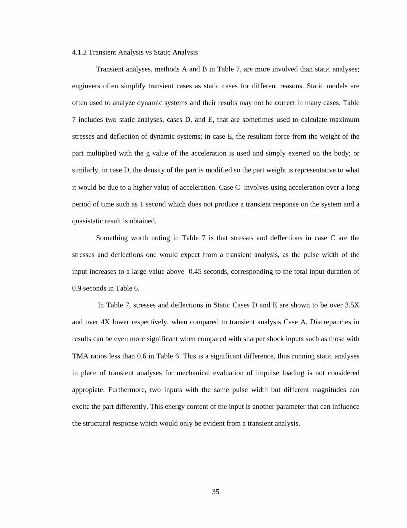
4.1.2 Transient Analysis vs Static Analysis ............................................................... 35

vii

4.2 Second Case Study: The I508 Inlet Guide Vane Housing (IGV)................................... 36

4.2.1 IGV Stresses and Deflections vs Direction of Shock ........................................ 37

4.2.2 I508 IGV Full Model ......................................................................................... 38

4.2.3 Evaluation of Maximum IGV Stresses and Deflections .................................... 39

4.2.4 Sensitivity of Pulse Width, IGV Axial Forward Direction ............................... 40

4.3 Third Case Study: Baseline Impeller Shock Analysis ................................................... 42

4.3.1 Baseline Impeller Shock Analysis By Finite Element Analysis ........................ 49

4.3.2 Baseline Impeller Undergoing Rotation and Shock, Two Solution Methods ... 53

4.3.3 Summary of Chapter 4 ...................................................................................... 63

CHAPTER 5: EXPERIMENTAL AND ANALYTICAL SHOCK TESTING OF THE H200 MIXED FLOW FAN ................................................................................................. 65

5.1 Analytical Results .......................................................................................................... 66

5.1.1 Impeller and Rotor Subassembly ...................................................................... 67

5.1.2 Front Bearing Housing ...................................................................................... 70

5.1.3 Fan Shroud ........................................................................................................ 71

5.1.4 Rolling Element Bearings ................................................................................. 73

5.1.5 Final Analytical Results for the Mixed Flow Fan ............................................. 77

5.2 Experimental Results for the H200 Mixed Flow Fan..................................................... 78

5.2.1 Fan Inspection After Shock Loading ................................................................. 82

5.3 Summary of Chapter 5 ................................................................................................... 84

CHAPTER 6: CONCLUSION ..................................................................................................... 86

REFERENCES .............................................................................................................................. 87

APPENDIX A: MATLAB CODE ................................................................................................ 89

viii

LIST OF TABLES Table Page

1. lβ Values ........................................................................................................................ 15 2. Comparison of Mode Shape Results By Different Methods ............................................ 23 3. Glass Panel Mechanical Properties .................................................................................. 29 4. Steel Fork Mechanical Properties .................................................................................... 29 5. Glass Panel Triangular Wave Input, 0.6 Second Period .................................................. 31 6. Glass Panel Stress and Deflection Sensitivity to Impulse Duration ................................ 33 7. Transient Cases A, B, C vs Static Cases D and E ............................................................ 36 8. Stress and Deformation Results for The I508 Simplified IGV Under 40 g of

Acceleration, 20 Vanes, X, Y, and Z Acceleration Inputs ............................................... 38 9. I508 IGV Full Model Under a 40 g Shock, All 37 Vanes, X, Y, and Z Acceleration

Inputs ............................................................................................................................... 39 10. High Resolution Results For the Dynamic Response of a Simplified IGV to a 40 g

Axial Forward Acceleration ............................................................................................. 41 11. Analytical and FEA Modal Results For The Baseline Impeller ...................................... 48 12. Table of Values for Figure 41 .......................................................................................... 53 13. MIL STD 810 Shock Requirements Using a Half Sine Input .......................................... 65 14. Impeller-Rotor Results for Maximum Deflection For A Ballistic Shock, Rotational

and Aerodynamic Loading Also Included ....................................................................... 70 15. FBH Results for Maximum Deflection For All Three Types of Shock (Inches) ............. 71 16. Maximum Deformation of Fan Shroud in the Fan Assembly .......................................... 72 17. Addition of All Radial Shock Deformation Results That Affect Tip Clearance ............. 78 18. Addition of All Axial Shock Deformation Results That Affect Tip Clearance ............... 78

ix

LIST OF FIGURES Figure Page 1. Ballistic Shock [20] ......................................................................................................... 5 2. Cyclone 100 Fan by Xcelaero Corporation...................................................................... 7 3. Impeller Blades have similar properties as Cantilevered Beams ..................................... 8 4. Cantilevered Beam Curvature [5] .................................................................................... 10 5. Photograph of the first four resonant frequencies of a PVC Beam used by Repetto,

Roatta, and Welti ............................................................................................................. 18 6. First Mode Shape of the PVC Cantilevered Beam .......................................................... 19 7. Second Mode Shape of the PVC Cantilevered Beam ...................................................... 20 8. Third Mode Shape of the PVC Cantilevered Beam ......................................................... 20 9. First Mode Shape of the PVC Cantilevered Beam, FEA Model...................................... 21 10. Second Mode Shape of the PVC Cantilevered Beam, FEA Model ................................. 22 11. Third Mode Shape of the PVC Cantilevered Beam, FEA Model .................................... 22 12. 18 Inch Long Cantilevered Beam with a 10 N Step Load ............................................... 24 13. Dynamic Response at the Free End of Cantilevered Beam from Classical Theory ......... 25 14. FEA Dynamic Solution for 18 Inch Long Cantilevered Beam with a 10 N Step Load ... 26 15. Comparison between FEA and Theoretical Results for an 18 Inch Long Cantilevered

Beam ................................................................................................................................ 27 16. 2.2 m x 2.5 m (7.2 ft x 8.2 ft) Glass Panel on a Lifting Fork ........................................... 28 17. Mesh of Glass Panel and Fork ......................................................................................... 30 18. Boundary Conditions of the Assembly ............................................................................ 30 19. Glass Panel Triangular Wave Input, 0.6 Second Period .................................................. 31 20. Deformation Probe at the Glass Corner ........................................................................... 32

x

21. Glass Panel Stress and Deflection Sensitivity to Impulse Duration ................................ 34 22. Stresses were evaluated on the Glass at the Corner Support, bottom right ...................... 34 23. A Crash Hazard Shock, a Half Sine Pulse with 40 g in 11 milliseconds ......................... 36 24. I508 IGV Simplified Model with 20 Vanes ..................................................................... 37 25. IGV Axial Forward Results, Maximum Stresses = 4.77 ksi ............................................ 40 26. IGV Axial Forward Acceleration, Maximum Radial Deformation over Impeller

Blades = 0.00017 inches .................................................................................................. 40 27. Simplified IGV Stress and Deflection Sensitivity to Impulse Duration, 40 g

Forward Shock, n = 1.7 ms. ............................................................................................ 41 28. Baseline Impeller, a Representative Impeller Mechanical Model ................................... 43 29. A Production Typical Propulsor Impeller ........................................................................ 43 30. First Resonant Frequency and Mode Shape of the Baseline Impeller Blade

Approximated as a Cantilevered Beam ............................................................................ 45 31. Second Resonant Frequency and Mode Shape of the Baseline Impeller Blade

Approximated as a Cantilevered Beam ............................................................................ 45 32. Third Resonant Frequency and Mode Shape of the Baseline Impeller Blade

Approximated as a Cantilevered Beam ............................................................................ 46 33. First Bending Mode of Blades at 448 Hz ......................................................................... 47 34. Second Bending Mode of Blades at 2751 Hz .................................................................. 47 35. Third Bending Mode of Blades at 7394 Hz ..................................................................... 48 36. Half Sine Acceleration Shock Input with a Positive Magnitude of 50 g and a

Pulse Width of 5 ms ......................................................................................................... 49 37. Meshed Baseline Impeller Model .................................................................................... 50 38. Maximum Baseline Impeller Response at the Blade Tips for a 50 g, 5 ms Input ............ 51 39. Baseline Impeller Undergoing a 50 g, 5 ms Shock Input, Deformed and

Undeformed Blades Shown ............................................................................................. 51

xi

40. Baseline Impeller Sensitivity to Pulse Width, 50 g Shock, τn = 2.2 ms .......................... 52 41. Initial Conditions for the Baseline Impeller Transient Analysis ...................................... 55 42. Probe Location for Axial Deformation Calculations ....................................................... 56 43. Full Baseline Impeller Model Solution for Axial Tip Deformation from Simultaneous

Rotation and Shock Loading ............................................................................................ 57 44. A Mode Superposition Model from Ansys Mechanical .................................................. 59 45. Static Analysis Performed as Part of Mode Superposition Method ................................. 59 46. Baseline Impeller Axial Deformation due to Rotation Only as Part of a

Superposition Three Step Solution .................................................................................. 60 47. Baseline Impeller Modal Frequency Solution under a Pre Stressed Condition ............... 61 48. Axial Deformation at the Probe from Final Results from a Mode Superposition

Solution ............................................................................................................................ 62 49. Axial Deformation Impeller Profile in the Final Results from a Mode Superposition

Solution ............................................................................................................................ 62 50. Cross Section of Mixed Flow Fan Assembly for Illustration Purposes ........................... 66 51. Impeller and Rotor Shaft Analysis Settings in Two Steps; Step 1 includes Rotation

and Aerodynamic Effects and Step Two includes the Ballistic Shock Input ................... 68 52. Impeller and Rotor Shaft Axial Deformation Results for the Axial Ballistic Shock,

Rotational and Aerodynamic Loading Also Included (the Rotor part is hidden) ............ 68 53. Impeller and Rotor Shaft Maximum Axial Deformation Results for the Axial Ballistic

Shock, Rotational and Aerodynamic Loading Also Included .......................................... 69 54. Impeller and Rotor Shaft Maximum Deformation Results for the Axial Ballistic

Shock Only ...................................................................................................................... 69 55. Front Bearing Housing Lateral Deformation due to the Lateral Ballistic Shock ............. 71 56. Fan Shroud Lateral Deformation from a Lateral Ballistic Shock, Highly Deformed

Model Shown for Illustration Purposes Only .................................................................. 73 57. Hertzian Contact between a sphere and a non-conforming surface [19] ......................... 74

xii

58. Ball Bearing Internal Clearances [17] .............................................................................. 76 59. Maximum Angular Displacement Measurement in a Single 10x26x8 mm Ball

Bearing ............................................................................................................................. 77 60. H200 Fan Instrumented with Accelerometers ................................................................. 79 61. Electromagnetic Shaker Table and EMIC Model F-2000-BC-E07 ................................. 79 62. Fan Response to Ballistic Shock in the Lateral Direction ............................................... 80 63. Fan Response to Gun Firing Shock in the Lateral Direction ........................................... 81 64. Fan Response to Road Load Shock in the Lateral Direction ........................................... 81 65. Light Scraping on the Fan Impeller ................................................................................. 82 66. Light Scrape Mark on Fan Shroud ................................................................................... 83 67. Inspection of Bearing Rings Showing Axial Brinells ...................................................... 84

xiii

NOMENCLATURE

Symbol/Abbreviation Description

A Cross section of the beam

An A constant

Bn A constant

C A constant

D Diameter

E Young's modulus of elasticity

Hz Hertz

Gpa Gigapascal

I Bending moment of inertia

M Bending moment

N Newtons

P Concentrated load

R Radius

T Thickness of the beam

Y(x) Displacement in space

W(t) Displacement in time

V Shear force

EI Flexural rigidity or bending stiffness

CG Center of gravity

FEA Finite element analysis

xiv

FBH Front bearing housing

GB Gigabytes

IGV Inlet guide vanes

LE Leading edges

OD Outside diameter

P Normal force

P0 Contact pressure

NSK A bearing manufacturer

RPM Revolution per minute

RAM Random access memory

TE Trailing edges

TMA Time to maximum acceleration

V V equation, explicit

W Watts

a Radius of contact

e Natural log

fn Natural frequency

g Gravity

in Inches

l Length of the cantilevered beam

lbf Pound force

m Mass, Meters

ml Mass per unit length

xv

mt Total mass

mm Millimeter

ms Milliseconds

t Time

tan Tangent

cos Cosine

cosh Hyperbolic cosine

psi Pounds per square inch

sin Sine

sinh Hyperbolic sine

w Width of the beam

β A constant

∆ Delta equation, explicit

θ Angle theta

⍴ Density

⍴c Radius of curvature

ε Strain

σ Stress

κ Curvature of the beam

ν Poisson's ratio

α Deflection

⍵n Circular natural frequency

1

CHAPTER 1

INTRODUCTION TO THE STUDY

1.1 Problem Formulation

Shocks are a prevalent loading condition that occur every day and affect simple

mechanical parts, complete mechanical assemblies such as military tanks, commercial products,

and even humans. Engineers use tools such as finite element modeling to analyze complex parts

and assemblies. More validation of analyses with experiments are necesary to master the solution

process of these complicated problems.

1.2 Purpose of the Study

The purposes of this study are to analyze shock loading using finite elements, validate the

process and results using simple and continuous structures, investigate the mechanical effects due

to variation pulse width in the acceleration input, and complete a transient analysis of a mixed

flow fan undergoing ballistic shock using knowledge gained from analyses of a simple

continuous structure.

The shock input is a half sine acceleration excitation; this type of input is very

representative of impulse loading for structures undergoing shocks such as those mentioned

above; other inputs also used for modeling real life shocks include "the decaying sinusoidal

acceleration, and the complex oscillatory-type motion [16]."

1.3 Limitations of the Study

Theoretical and finite element analysis were conducted at standard ambient conditions

and using constant isotropic material properties. Mechanical effects of shock loading for the

mixed flow fan are compared in terms of radial and axial deformations that would cause total

closure of the impeller tip clearance.

2

1.4 Literature Review

An extensive amount of sources were reviewed for the completion of this study on shock

loading; for brevity, only the most prominent sources are included in this literature review. The

areas that these sources cover include, but are not limited to, background information on shock

loading, theory and governing equations for basic structures such as cantilivered beams,

experiments involving natural frequencies and acceleration inputs, finite element modeling using

Ansys Workbench, and Hertz contact theory and analysis. Understanding shock loading and

modeling this condition using finite elements was accomplished by learning to solve the

governing equations of basic structures such as beams, validating results with experimental data,

and running FE models of simple and complex structures.

In " Euler-Bernoulli Beams" [5] Terje Haukaas derives the governing beam differential

equation for Euler-Bernoulli type beams using equilibrium and section integration, material law,

and kinematics. In "Vibrations of Cantilever Beam, Deflection, Frequency, and Research Uses"

[7] Scott Whitney clearly states the steps to arrive at the general solution of the beam equation

for a cantilevered beam. These are the primary sources for deriving and solving the governing

beam equation. These provide natural frequencies and mode shapes of cantilevered beams which

are compared to experimental solutions.

In "Forced Vibration of a Cantilever Beam" [4] C. E. Repetto, et. al, present modal

experimental results for a 0.50 m long PVC beam that is held vertically, and excited by a wave

driver; the transverse natural frequencies are measured to be

ω = 7.79, 36.44, 97.39, and 185.35 s-1. Except for the fundamental frequency which was

influenced significantly by gravity effects and damping, these results were found to be within 9%

error compared to their theoretical results and within 10% error when compared to the theoretical

results in this report. In this experiment, using a ferrous metal would have eliminated any

damping that occurs with the PVC material and would have simplified the experimental and

3

analytical comparisons. The same Euler-Bernoulli governing differential equations are used in the

dynamic solution of beams undergoing forced vibration, specifically shock loading.

In "Stress, Strain, and Structural Dynamics: An Interactive Handbook of Formulas,

Solutions, and Matlab Toolboxes" [12] Bingen Yang provides a program for the dynamic analysis

of beams; he explains how to set up beam types, boundary and initial conditions, damping,

response time, and output control. The program can solve for mode shapes of Euler-Bernoulli

beams; it can solve for the beam's response in time and space as well as its internal forces. Modal

damping can also be specified to filter out higher frequencies in the response. Input of external

forces is also possible using this program. Static analysis of Euler-Bernoulli beams is also

covered which provides useful background information prior to evaluating dynamic analysis. The

governing equations and analytical solution derivations are also included. The theoretical

response for a cantilevered beam undergoing shock is obtained; the finite element analysis of the

same model, as presented in this report, closely matches the theoretical reponse. This resource is

extremely valuable in validating the FEA cantilevered beam model and is the basis for analyzing

comlex parts and assemblies. One of these assemblies is a glass panel and steel fork assembly.

In "Finite Element Simulations with ANSYS Workbench 14" [1] Huei-Huang Lee

presents an Ansys tutorial based on a glass planel and lifting fork which provided the basic

knowledge for FEA transient analysis of shock loading of this system. When the glass panel is

moved up or down with accelerations of approximately 4 g, the tips of the glass panel deflect for

some amount of time; for this system it is important to know when the deflections have decayed

so the glass panel can be inserted into the processing machine. Every step is carefully detailed

from beginning to end including screen shots of each step. Geometry and material properties for

the glass panel and the steel fork are provided. The contact is specified as bonded, the glass is

mapped meshed and the steel fork is meshed with a thin sweep using solid shell elements. Step

controls, damping, boundary conditions, initial conditions, and post-processing are also clearly

described. This source provides an excellent introduction for modeling shock loading using finite

4

elements. FEA analysis using Ansys proves to be a very capable tool for shock analysis even at

the assembly and subassembly levels. A subassembly that was difficult to analyze was the ball

bearing.

In "Fundamentals of Machine Component Design" [18] Robert Juvinal and Kurt Marshek

present the Hertz contact theory for curved surfaces such as bearings where finite contact points

and lines exist. Very high contact stresses can develop in these areas and often times it involves a

cyclic type loading where loading and unloading occurs with high frequency. Surface fatigue

develops and eventually leads to fatigue failure. The authors describe the applicable equations in

term of Poisson's ratio, Young modulus, and radii of the applicable parts. The assumptions that

apply are listed as well as the type of stresses involved on the surfaces as well as beneath them.

Other factors to consider are also discussed such as thermal expantion and hydrodynamic

pressure. However, it is necessary to find information on deflection formulas in other sources.

Understanding shock loading and modeling this condition using finite elements is

accomplished by learning to solve the governing equations of basic structures such as beams,

validating results with experimental data, and running FE models of simple and complex

structures. Experimental data was found for a cantilevered beam; this was analyzed and compared

to theoretical results. Then a test case involving a glass panel exposed all the different parts of

modeling complex structrues using an FEA code such as Ansys Workbench. A mixed flow

machine is the largest and most complex assembly analyzed with finite elements; Hertz contact

theory is also used to analyze complex components such as ball bearings. Every reference is vital

in building the knowledge base and tools for understanding and solving engineering problems

involving shock loading.

5

CHAPTER 2

PREVALENCE OF SHOCK LOADING AND THE EULER-BERNOULLI THEORY

2.1 Background

Mechanical shocks are a very common occurrence in everyday life; examples of shock

loading include explosions, car hitting a pothole, reciprocating engine fuel explosions inside

cylinders, airplane landing, bolted joints suddenly opening and closing with an impact, high

winds can be a source of step loading, earthquakes, drop impact during handling, g forces

generated for internal components, high speed fluid entry, etc. "When the load increases to its

maximum value over five or six natural periods, it is a quasi-static load. When it does so over a

fraction of the period, it is a shock loading. Broader definitions exist, where anything with up to

two periods duration is a shock loading [2]."

Figure 1. Ballistic Shock [20].

6

Shock analysis has become a requirement with specific customer guidelines to follow

during the design process as well as in the testing qualification phase of products in many

industries, including high performance cooling fans, which is the basis of the last chapter in this

report. Thus it is important in the preliminary and critical design phase to appropriately run

analytical and finite element models that predict safe operation of these machines. In the

qualification phase, specific high level shocks are applied; it is crucial that all components inside

the machine withstand these shocks and continue to function satisfactorily and safely. Shock

levels inside military aircraft and vehicles are related to human tolerance for acceleration

changes. In 1955, Col. John Stapp determined that a person can survive a deceleration of 46.2 g

in 1.4 seconds [21]. For acceleration levels of up to 50 g, the input duration should not be any

more than 50 ms, otherwise severe injury can occur [22]. This could be one of the limiting factors

and the reason why only shocks of low magnitude are allowed inside the crew compartment of

military vehicles.

A possible mechanical effect during shock loading is that an impeller or wheel tip

deflection is such that it collides with its inlet or inlet shroud for any type of fan or rotating

machinery with tight tip clearances. Figure 2 shows a vane axial fan with a tight clearance

between the rotating and stationary components. This collision must be prevented to avoid any

risk of impeller blade rupture. The dynamics of the rotor and shroud response must be carefully

understood to properly design all components while making the right compromises between

materials, wall thickness, weight, design features, etc.

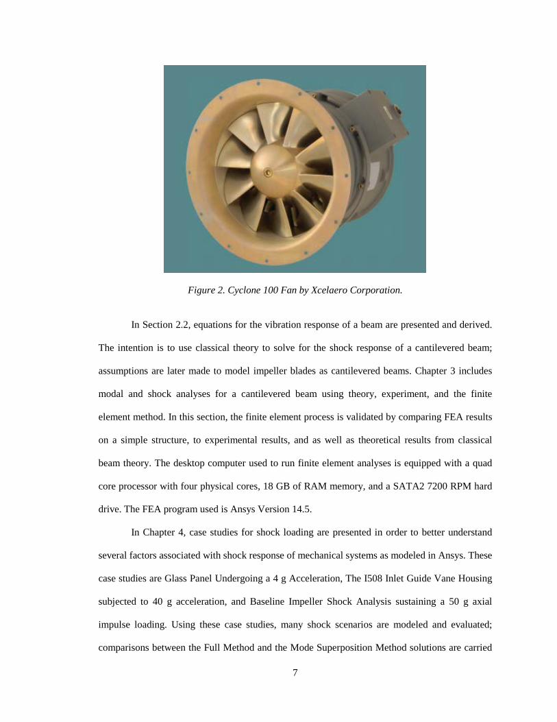
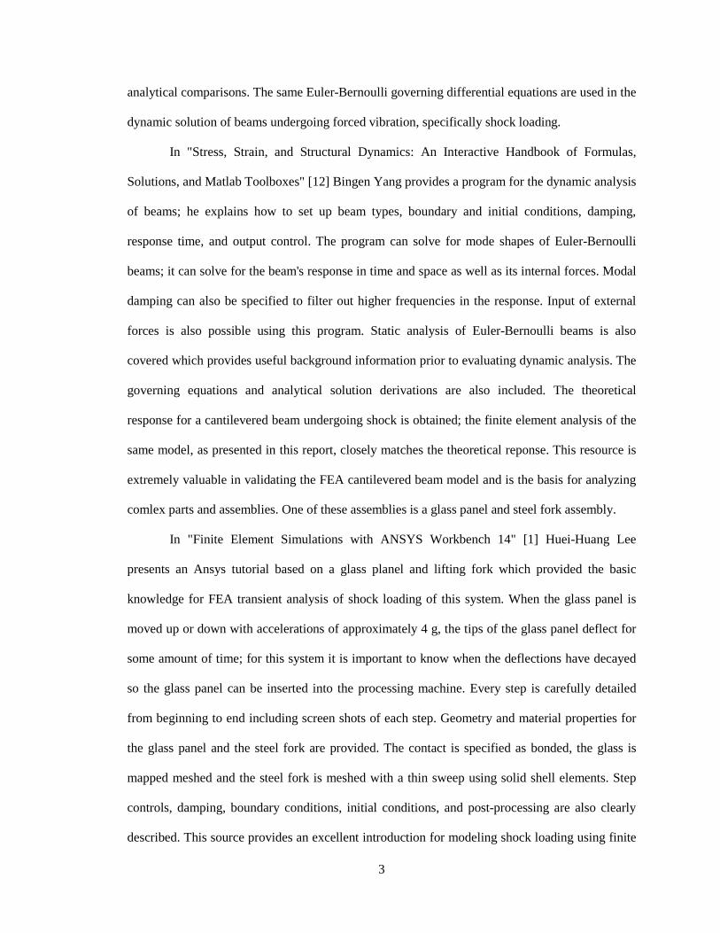
7

Figure 2. Cyclone 100 Fan by Xcelaero Corporation.

In Section 2.2, equations for the vibration response of a beam are presented and derived.

The intention is to use classical theory to solve for the shock response of a cantilevered beam;

assumptions are later made to model impeller blades as cantilevered beams. Chapter 3 includes

modal and shock analyses for a cantilevered beam using theory, experiment, and the finite

element method. In this section, the finite element process is validated by comparing FEA results

on a simple structure, to experimental results, and as well as theoretical results from classical

beam theory. The desktop computer used to run finite element analyses is equipped with a quad

core processor with four physical cores, 18 GB of RAM memory, and a SATA2 7200 RPM hard

drive. The FEA program used is Ansys Version 14.5.

In Chapter 4, case studies for shock loading are presented in order to better understand

several factors associated with shock response of mechanical systems as modeled in Ansys. These

case studies are Glass Panel Undergoing a 4 g Acceleration, The I508 Inlet Guide Vane Housing

subjected to 40 g acceleration, and Baseline Impeller Shock Analysis sustaining a 50 g axial

impulse loading. Using these case studies, many shock scenarios are modeled and evaluated;

comparisons between the Full Method and the Mode Superposition Method solutions are carried

8

out. The sensitivity studies conducted include using static analysis in place of transient analysis,

effectiveness of modeling impeller blades as cantilevered beams, and effects of varying pulse

widths of the acceleration input. Finally, in Chapter 5, lessons learned in Chapters 2, 3, and 4 are

put into practice in the evaluation of shock loading for a mixed flow fan subjected to a maximum

shock of 50 g. Damping effects are neglected in all structural cases considered except in the Glass

Panel Case.

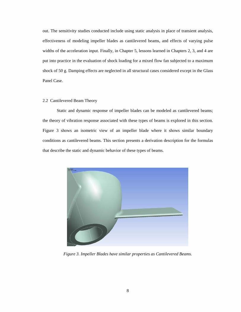
2.2 Cantilevered Beam Theory

Static and dynamic response of impeller blades can be modeled as cantilevered beams;

the theory of vibration response associated with these types of beams is explored in this section.

Figure 3 shows an isometric view of an impeller blade where it shows similar boundary

conditions as cantilevered beams. This section presents a derivation description for the formulas

that describe the static and dynamic behavior of these types of beams.

Figure 3. Impeller Blades have similar properties as Cantilevered Beams.

9

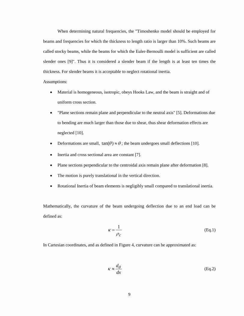
When determining natural frequencies, the "Timoshenko model should be employed for

beams and frequencies for which the thickness to length ratio is larger than 10%. Such beams are

called stocky beams, while the beams for which the Euler-Bernoulli model is sufficient are called

slender ones [9]". Thus it is considered a slender beam if the length is at least ten times the

thickness. For slender beams it is acceptable to neglect rotational inertia.

Assumptions:

• Material is homogeneous, isotropic, obeys Hooks Law, and the beam is straight and of

uniform cross section.

• "Plane sections remain plane and perpendicular to the neutral axis" [5]. Deformations due

to bending are much larger than those due to shear, thus shear deformation effects are

neglected [10].

• Deformations are small, tan( )θ θ≈ ; the beam undergoes small deflections [10].

• Inertia and cross sectional area are constant [7].

• Plane sections perpendicular to the centroidal axis remain plane after deformation [8].

• The motion is purely translational in the vertical direction.

• Rotational Inertia of beam elements is negligibly small compared to translational inertia.

Mathematically, the curvature of the beam undergoing deflection due to an end load can be

defined as:

1

cκ

ρ= (Eq.1)

In Cartesian coordinates, and as defined in Figure 4, curvature can be approximated as:

dxdθκ ≈ (Eq.2)

10

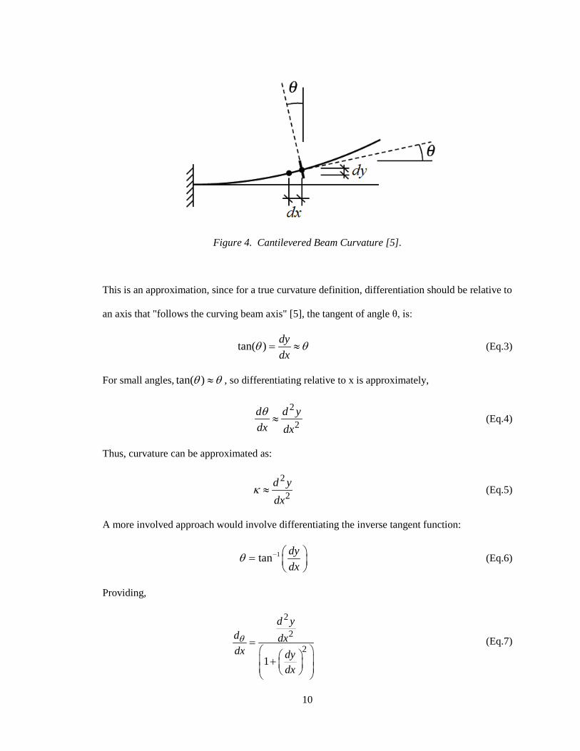
Figure 4. Cantilevered Beam Curvature [5].

This is an approximation, since for a true curvature definition, differentiation should be relative to

an axis that "follows the curving beam axis" [5], the tangent of angle θ, is:

tan( ) dydx

θ θ= ≈ (Eq.3)

For small angles, tan( )θ θ≈ , so differentiating relative to x is approximately,

2

2d d ydx dxθ

≈ (Eq.4)

Thus, curvature can be approximated as:

2

2d ydx

κ ≈ (Eq.5)

A more involved approach would involve differentiating the inverse tangent function:

1tan dydx

θ − =

(Eq.6)

Providing,

2

2

21

d

dx dydx

yd dxθ =

+

(Eq.7)

11

When the curvature of the beam is small, dydx

is small and ddxθ can be approximated as shown in

equation (Eq.4), "from mathematics, the exact curvature expression for the exact curvature is"

[5]:

2

23/22

1

d

dxdydx

yd dxθκ ≈ =

+

(Eq.8)

Where ⍴c is the beam's radius of the curvature,

xc

yερ

= (Eq.9)

Per Hook's Law and linear elastic theory:

x xEσ = ò (Eq.10)

Combining equations (Eq.8), (Eq.9) and (Eq.10):

x

cy

Eyσ

κρ

= = (Eq.11)

Re-arranging,

xyEσκ = (Eq.12)

From beam theory,

xMyI

σ = (Eq.13)

Substituting equation (Eq.13) into equation (Eq.12):

1MyyEI

κ = (Eq.14)

12

After canceling terms:

MEI

κ = (Eq.15)

Substituting equation (Eq.5) into equation (Eq.15):

2

2d yM EIdx

= (Eq.16)

From equilibrium and section integration of a differential section of a loaded beam, the resultant

shear force can be defined as the second derivative of the moment in space:

2

2

4

4yEI

dxd M d

dx= (Eq.17)

The differential equation that describes the dynamic transverse forced behavior of a cantilevered

beam is:

( )2 4

2 4,y ym EI f x t

t x∂ ∂

+ =∂ ∂

(Eq.18)

Equation (Eq.18) above is solved by separation of variables, and using a new set of variables Y

and W for clarity,

( , ) ( () )y x t Y Wx t= (Eq.19)

Let us solve equation (Eq.18) for a cantilevered beam undergoing free vibration, ( ), 0f x t = ,

thus equation (Eq.18), simplifies to:

4

2 4

2 0y ym EIt x

∂ ∂+ =

∂ ∂ (Eq.20)

Equation (Eq.20) becomes:

2 4

2 4( , ) ( , )y x t y x tm EIt x

∂ ∂− =

∂ ∂ (Eq.21)

2 4

2 4( ( ))( ) ( )( ( ))Y x Y xm EI

t xW t W t∂ ∂

− =∂ ∂

(Eq.22)

13

Dividing (Eq.22) by Y(x)W(t) ,

2

2 4

41 ( )( )

()

)(

EI Y xW t mY x

tt

Wx

∂ ∂− =

∂ ∂ (Eq.23)

Let's define the natural circular frequency as:

2n

ImEω = (Eq.24)

Both the left and right side of equation (Eq.23) are independent of each other; the left

side is differentiated in time and becomes equal to a constant; in a similar way the right side is

differentiated in space and equals a constant. "Because each side equals a constant, [equation

(Eq.23)] is valid and the method of separation of variables can be used. Let this constant be

denoted 2nω "

Defining,

2

4 n mEI

ωβ = (Eq.25)

When separation of variables is applied, equation (Eq.23), which is a fourth order differential

equation, becomes two ordinary differential equations [23]. Equation (Eq.23) and in conjunction

with (Eq.25) become:

4

4 ( ) 0x

d Y Y xd

β− = (Eq.26)

And

2

22

) ( ) 0(n

ddtW t W tω+ = (Eq.27)

Deflection mode shapes are found by solving equations above and using appropriate boundary

conditions for a cantilevered beam; such boundary conditions are:

At the clamped end, (0) 0y = , (0) 0xd

yd= (Eq.28)

14

At the free end, 2

2(l) (l) 0M EI ydxd

= = , 3

3V(l) (l) 0EI ydxd

= = (Eq.29)

The general solutions for equations (Eq.26) and (Eq.27) are "linear combinations of trigonometric

equations" [6, 7]:

1 2 3

4

( ) [cos( ) cosh( )] [cos( ) cosh( )] [sin( ) sinh( )][sin( ) sinh( )]

Y x C x x C x x C x xC x x

β β β β β ββ β

= + + − + +

+ − (Eq.30)

( )5 6(sin(( ) ) cosW t C t C tω ω= + (Eq.31)

After applying boundary conditions to equation (Eq.30) and its derivatives

dYdx

, 2

2d Ydx

, and 3

3d Ydx

(Eq.32)

We are able to solve for the C coefficients,

from (0) 0y = , 1 0C = (Eq.33)

from 0dydx

= , 3 0C = (Eq.34)

(Eq.30), (Eq.33), and (Eq.34) can be combined, and solved for 4C :

4 2cos( ) cosh( )sin( ) sinh( )

l lC Cl l

β ββ β

− −=

+ (Eq.35)

Combining (Eq.30) and (Eq.35), we obtain:

2cos( ) cosh( )(x) ][sin( x) sinh( x)]}sin( ) sinh

{[cos( ) cosh [)

x](

( l lY Cl l

x β β β ββ β

β β −−= −

++

−

(Eq.36)

"in order for the dynamic solution for the displacement to be equal to the static solution, at t=0,

C2 must be equal to 1/2.

2

12

C = (Eq.37)

15

Using this value of C2 in equation (Eq.36), we obtain:

Y(0) = 0 and Y(l)= -1 (Eq.38)

Combining equation (Eq.35) with 2

2d Ydx

or 3

3d Ydx

, and substituting the trigonometric identities:

2 2sin cos 1+ = and 2 2cosh sinh 1− = , provide:

cos( ) cosh( ) 1l lβ β = − (Eq.39)

Which is "the frequency equation for a cantilever beam" [7].

This nonlinear equation (Eq.39) "must be solved numerically to determine allowable

values of lβ , there are an infinite number of solutions corresponding to the possible modes of

vibration"[24]. "The system has infinite frequencies. It is continuous, and all continuous systems

have infinite number of frequencies [6]." Table 1 below shows values of lβ for the first four

natural frequencies. "These mode shapes are also called eigenfunctions [6]."

Table 1. lβ Values

n lβ

1 1.8751

2 4.6940

3 7.8547

4 10.9955

Using lβ values in Table 1, we can now solve for circular natural frequencies using the following

explicit equation:

( ) ( )2 23 3n

l

EI EIl lm l Al

ω β βρ

== (Eq.40)

16

Remember that m is mass per unit length in equation (Eq.40); to use total mass, the equivalent

equation would be

( )23n

t

EIlm l

ω β= (Eq.41)

The formula for converting circular natural frequency into natural frequency in hertz is:

2

nnf

ωπ

= (Eq.42)

Furthermore, "for each frequency there exists a characteristic vibration" [7]. Thus in order to

determine the beam's response in space and time due to some initial conditions, the following

equation can be used:

( ) ( ) cos( ) si[ n(, )]n nn ny x t Y x BA t tω ω= + (Eq.43)

"Where nA depends on the initial position at t=0, and nB depends on the initial velocity [7]."

When the beam initial displacement is zero, 0nB = . nA can be found using the following

integral:

( )0

2 ( , 0) Y( )l

nA y x tl

x dx= =∫ (Eq.44)

Equation (Eq.44) "can be solved analytically by a computer math program" [7], resulting in the

following solution for nA ,

2 34 2

3 2 2

4{3sin( )(e +1)-2( ) e

EIm (sin( )e e 1)

cos( ( 1) 3)[3 ) (e e ]}

L ll ln

l l

PlA l l

l

l l

β ββ β

β β

β ββ β

β β

=

+ −

+

+− −

(Eq.45)

17

CHAPTER 3

VALIDATION OF ANSYS MODEL USING ANALYTICAL AND EXPERIMENTAL

RESULTS FOR SHOCK AND MODAL ANALYSES OF CANTILEVERED BEAMS

"Models based on beam-like elements with different boundary conditions, can be used to

simulate the response of structures in engineering applications” [4] such as bridges, cranes,

airplane wings, etc. In this section, the finite element process is validated by comparing FEA

results on a simple structure and comparing these with theoretical results from classical beam

theory. Modal and shock analyses are carried out in this section. Modal Analysis for impeller

blades can be approximated using a much simpler structure such as a cantilevered beam; at the

very least, solving for the modal solutions for this kind of beam serves as a good initial step

towards defining the mode shapes of impeller blades. Theoretical, experimental, and finite

element results will be compared and evaluated. Furthermore, shock analysis of a cantilevered

beam is also studied and compared to theoretical results; the same approach is later used for

analyzing impellers undergoing shock loading.

The cantilevered beam that will be used for comparison purposes is a PVC beam used by

Repetto, Roatta, and Welti in 2012 to experimentally determine the mode shapes at low

frequencies. A photograph of this beam during the experiment is shown in Figure 5. This same

beam is analyzed theoretically also using the finite element method. Its mechanical properties

include a Young's modulus of 3.1x109 Pa and a density of 1420 kg/m3. The beam's length,

l = 0.502 m, its width, w = 1.7x10-3 m, and its thickness, T = 0.89x10-3 m [4]. Bending stiffness,

EI, calculates to 3.096x10-4 N·m2. The beam is held vertically downward, including a fixed

support at the top and free at the bottom end; this helps in minimizing the directionality effect of

gravity. The shaker uses a transverse displacement to load the beam at different resonant

frequencies. An interesting independent finding by Repetto, Roatta, and Welti is that resonant

frequencies for the boundary conditions shown here "increase due to the stiffening effect of the

18

beams weight" exerting tension in the structure. Likewise, the opposite outcome is true for the

beam held in the opposite configuration. Furthermore, the gravitational effect is "found to mainly

influence the systems' response to the fundamental frequency of oscillation [4]".

Figure 5. Photograph of the first four resonant frequencies of a PVC Beam used by Repetto, Roatta, and Welti.

3.1 Theoretical Analysis of the PVC Cantilevered Beam

The Euler-Bernoulli beam theory found in the previous section was used to carry out

modal analysis of the PVC beam. Results from analysis will be compared to the experimental

results. A mathematical code was created in Matlab to solve for the first three eigen values and

eigen functions or mode shapes. The core of this program involves solving for equations (Eq. 35)

and (Eq. 36) using constants in Table 1. Input values that the code prompts for include the beam's

length, width, thickness, modulus of elasticity, and its density. The program uses two FOR loops

19

to solve for the spatial vertical deflections of the beam as a function of the beam span. Values of

the vertical axis are normalized relative to the maximum vertical value calculated for each mode;

units for the horizontal axis are meters and the mode frequencies calculated are in hertz.

Appendix A includes the Matlab code used to solve and graph the mode shapes of cantilevered

beams; results for the PVC beam are included in Figures 6 through 8. This theoretical code has

been used successfully in the process of impeller design, to quickly estimate mode shapes of

blades, as an efficient preliminary step to study resonance frequencies and construct Campbell

diagrams. These theoretical results were also validated using a separate toolbox by Bingen Yang

[12].

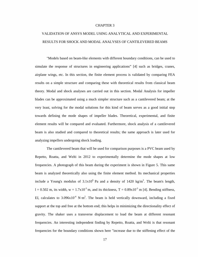
Figure 6. First Mode Shape of the PVC Cantilevered Beam.

20

Figure 7. Second Mode Shape of the PVC Cantilevered Beam.

Figure 8. Third Mode Shape of the PVC Cantilevered Beam.

21

3.2 FEA Analysis of the PVC Cantilevered Beam

FEA results of modal analysis of the PVC beam are included next. Models that are

symmetrical across one or more planes sometimes can be divided and reduced to the most

elemental form to save computational time. For this case, however, the model is small enough

and does not need simplification. Furthermore, using only a section of complete models is not

recommended for modal analysis; for instance, deciphering legitimate mode frequencies and

mode shapes becomes more involved. The full PVC beam model was used in this modal analysis.

The FEA analysis presented here does not take into account the effect of gravity; for this model, it

is considered negligible. This FEA model does not include any pre-stressed condition, it includes

a native Creo Parametrics model, and the relevant mechanical properties for PVC. Modal results

for total deformation are shown in Figures 9 through 11; they include the first in-plane or

transverse mode shapes and frequencies. These are also compared to experimental and analytical

results in Table 2.

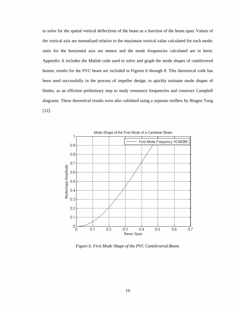
Figure 9. First Mode Shape of the PVC Cantilevered Beam, FEA Model.

22

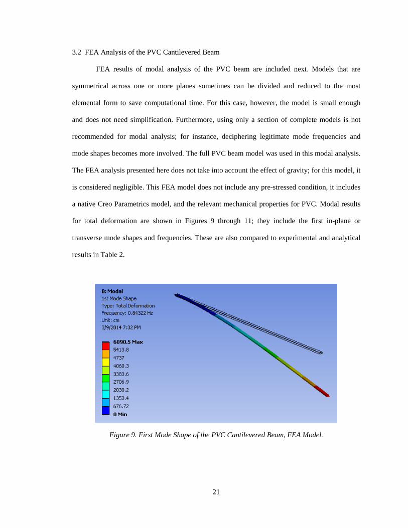
Figure 10. Second Mode Shape of the PVC Cantilevered Beam, FEA Model.

Figure 11. Third Mode Shape of the PVC Cantilevered Beam, FEA Model.

Table 2 includes a comparison between experimental results and theoretical values; the

second and third mode frequencies have less than 10% error. However, the fundamental

frequency has a discrepancy that is quite large; a probable cause could be that the deflection due

to gravity could be stiffening the beam and increasing its first resonance frequency, thereby

showing more sensitivity to gravity than the others.

23

Table 2. Comparison of Mode Shape Results By Different Methods.

Modes Shapes

Repetto, Roatta, Welti

Experiment

Theoretical Results 1 Matlab

Theoretical Results 2 Yang's Matlab

Toolbox

FEA Results

Experimental Results

Relative to Theoretical Results 1

(% Difference)

FEA Results Relative to Theoretical Results 1

(% Difference)

fn (Hz) 1st 1.24 0.843 0.843 0.843 47.07% 0.00% 2nd 5.80 5.283 5.284 5.284 9.78% 0.02% 3rd 15.50 14.796 14.796 14.796 4.76% 0.00%

ω (/s) 1st 7.79 5.297 5.298 5.297 47.07% 0.00% 2nd 36.44 33.194 33.202 33.200 9.78% 0.02% 3rd 97.39 92.966 92.965 92.966 4.76% 0.00%

What we want to start defining is how accurate the finite element method solves for the

modes and vibration response of simple structures, such as beams. In comparing FEA modal

analysis results to the theoretical results from the Matlab code, the last column in Table 2 shows

that these two are almost identical, with differences between 0.00% and 0.02%, which validates

this process for this cantilevered beam when compared against classical beam theory.

3.3 Shock Analysis of A Cantilevered Beam

Next, we evaluate the dynamic response of a cantilevered beam as modeled by finite

element analysis and classical theory. In Chapter 4, impeller blades are modeled as cantilevered

beams; thus, these results will be useful in this report. For this case, the cantilevered beam's

geometry is as follows: Length = 18 inches long (0.4572 m), width = 2 inches (50.800 mm), and

thickness = 0.0775 inches (1.969 mm). Material is aluminum with modulus of elasticity

E = 10.298x106 psi (71.002 Gpa) and a density ρ = 0.10015 lbf/in3 (2272 Kg/m3). Bending

stiffness EI = 798.929 in·lbf (2.2948 N·m) by calculation. A 10 N force is step applied mid-span

of the beam, at the center. "The acceleration impulse and the acceleration step are the classical

24

limiting cases of shock motion [16]." Figure 12 shows the boundary conditions and loading; the

beam response is tracked at the free end.

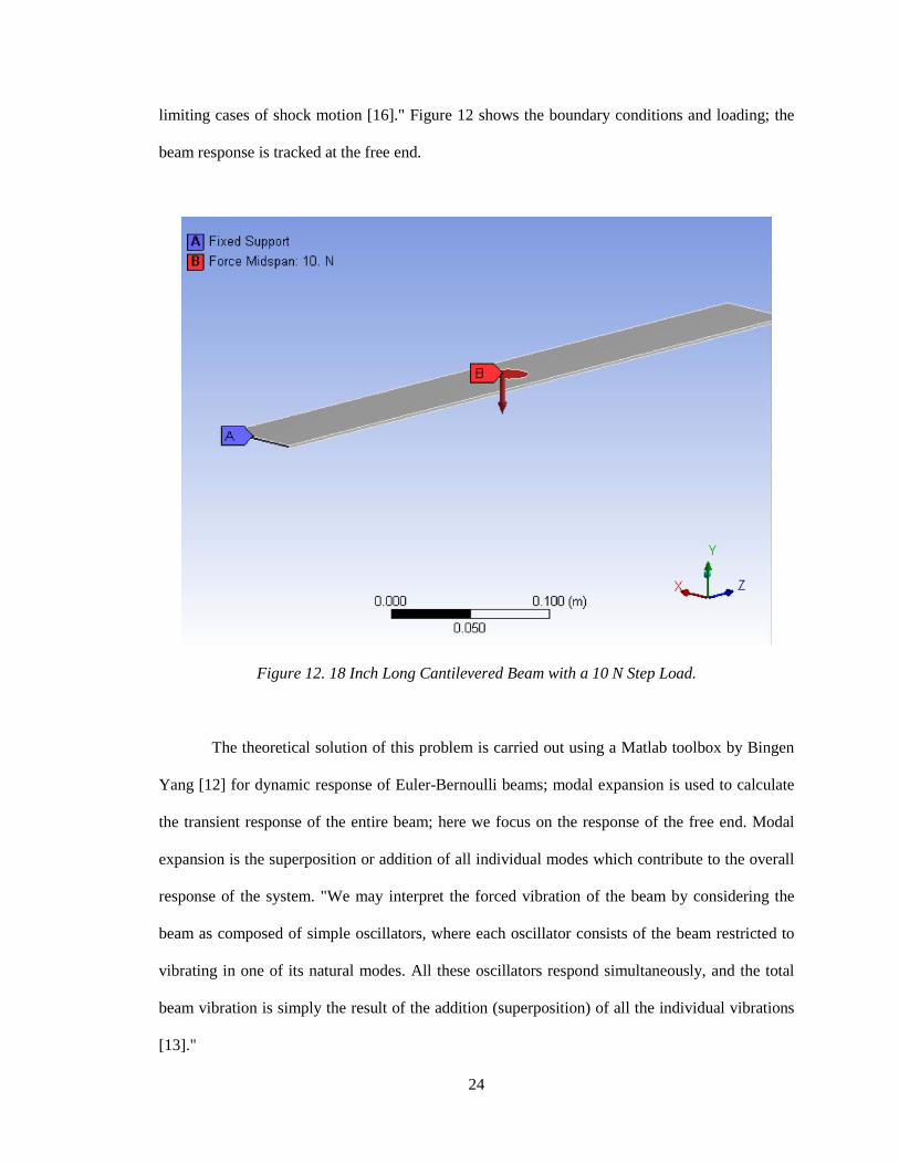
Figure 12. 18 Inch Long Cantilevered Beam with a 10 N Step Load.

The theoretical solution of this problem is carried out using a Matlab toolbox by Bingen

Yang [12] for dynamic response of Euler-Bernoulli beams; modal expansion is used to calculate

the transient response of the entire beam; here we focus on the response of the free end. Modal

expansion is the superposition or addition of all individual modes which contribute to the overall

response of the system. "We may interpret the forced vibration of the beam by considering the

beam as composed of simple oscillators, where each oscillator consists of the beam restricted to

vibrating in one of its natural modes. All these oscillators respond simultaneously, and the total

beam vibration is simply the result of the addition (superposition) of all the individual vibrations

[13]."

25

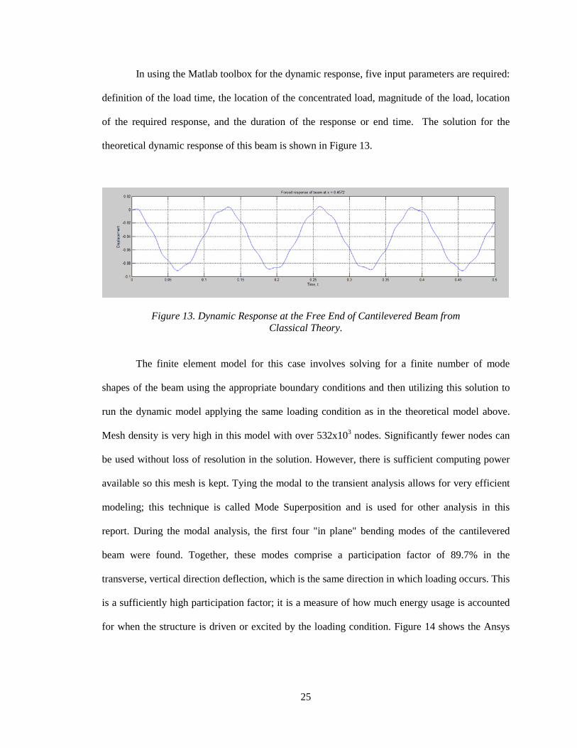
In using the Matlab toolbox for the dynamic response, five input parameters are required:

definition of the load time, the location of the concentrated load, magnitude of the load, location

of the required response, and the duration of the response or end time. The solution for the

theoretical dynamic response of this beam is shown in Figure 13.

Figure 13. Dynamic Response at the Free End of Cantilevered Beam from Classical Theory.

The finite element model for this case involves solving for a finite number of mode

shapes of the beam using the appropriate boundary conditions and then utilizing this solution to

run the dynamic model applying the same loading condition as in the theoretical model above.

Mesh density is very high in this model with over 532x103 nodes. Significantly fewer nodes can

be used without loss of resolution in the solution. However, there is sufficient computing power

available so this mesh is kept. Tying the modal to the transient analysis allows for very efficient

modeling; this technique is called Mode Superposition and is used for other analysis in this

report. During the modal analysis, the first four "in plane" bending modes of the cantilevered

beam were found. Together, these modes comprise a participation factor of 89.7% in the

transverse, vertical direction deflection, which is the same direction in which loading occurs. This

is a sufficiently high participation factor; it is a measure of how much energy usage is accounted

for when the structure is driven or excited by the loading condition. Figure 14 shows the Ansys

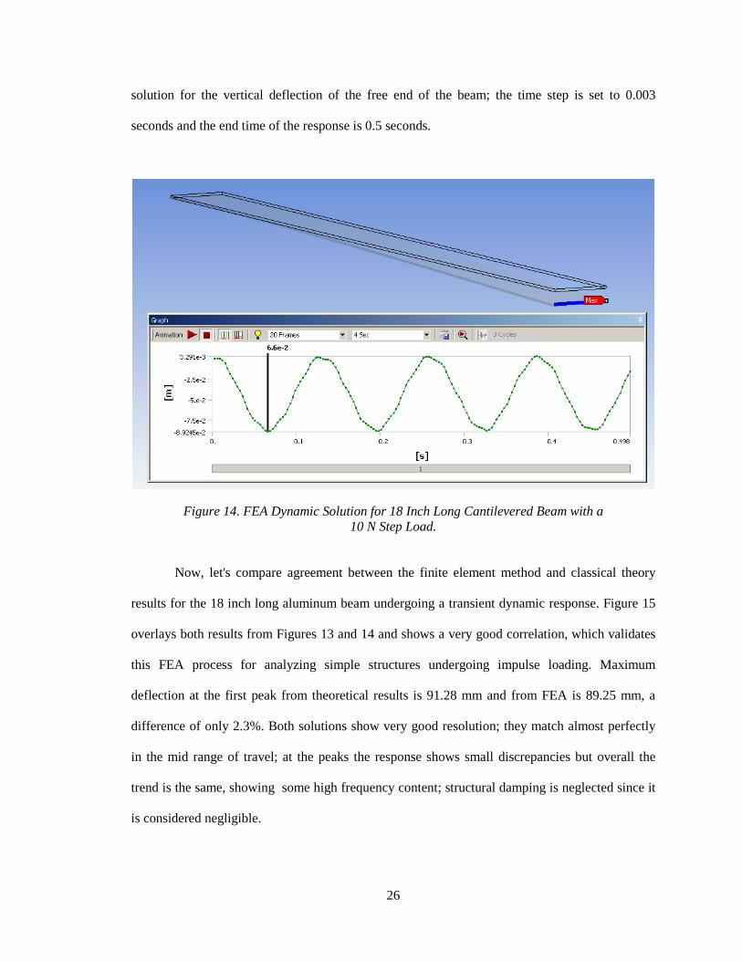
26

solution for the vertical deflection of the free end of the beam; the time step is set to 0.003

seconds and the end time of the response is 0.5 seconds.

Figure 14. FEA Dynamic Solution for 18 Inch Long Cantilevered Beam with a 10 N Step Load.

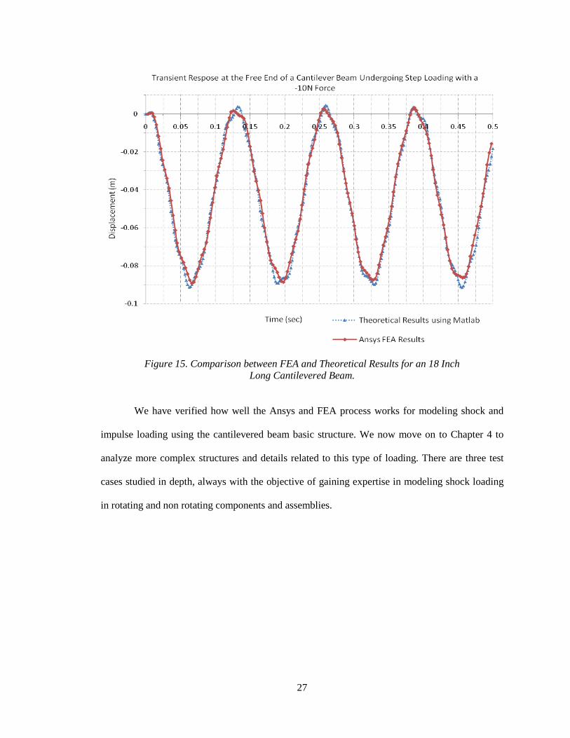
Now, let's compare agreement between the finite element method and classical theory

results for the 18 inch long aluminum beam undergoing a transient dynamic response. Figure 15

overlays both results from Figures 13 and 14 and shows a very good correlation, which validates

this FEA process for analyzing simple structures undergoing impulse loading. Maximum

deflection at the first peak from theoretical results is 91.28 mm and from FEA is 89.25 mm, a

difference of only 2.3%. Both solutions show very good resolution; they match almost perfectly

in the mid range of travel; at the peaks the response shows small discrepancies but overall the

trend is the same, showing some high frequency content; structural damping is neglected since it

is considered negligible.

27

Figure 15. Comparison between FEA and Theoretical Results for an 18 Inch Long Cantilevered Beam.

We have verified how well the Ansys and FEA process works for modeling shock and

impulse loading using the cantilevered beam basic structure. We now move on to Chapter 4 to

analyze more complex structures and details related to this type of loading. There are three test

cases studied in depth, always with the objective of gaining expertise in modeling shock loading

in rotating and non rotating components and assemblies.

28

CHAPTER 4

CASE STUDIES OF SHOCK LOADING

The motivation for conducting these studies is to gain experience with behavior of more

complex mechanical systems, using the same acceleration magnitude input, but varying the

duration of the pulse. Another objetive is to understand, in relative terms, the implications when

simplifying transient shock analysis as static analysis. This simplification is made, sometimes for

lack of knowledge in performing transient analyses, or as an initial step to save time, etc. This

exercise is found in Huei-Huang Lee's book [1], which provides significant information for

conducting shock analysis.

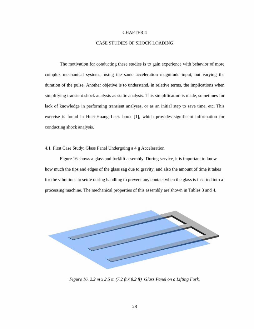
4.1 First Case Study: Glass Panel Undergoing a 4 g Acceleration

Figure 16 shows a glass and forklift assembly. During service, it is important to know

how much the tips and edges of the glass sag due to gravity, and also the amount of time it takes

for the vibrations to settle during handling to prevent any contact when the glass is inserted into a

processing machine. The mechanical properties of this assembly are shown in Tables 3 and 4.

Figure 16. 2.2 m x 2.5 m (7.2 ft x 8.2 ft) Glass Panel on a Lifting Fork.

29

Table 3. Glass Panel Mechanical Properties.

Glass Panel

Density (Kg/m3) 2370

Young's modulus (GPa) 70

Poisson's ratio 0.22

Table 4. Steel Fork Mechanical Properties.

Steel Fork

Density (Kg/m3) 7850

Young's modulus (GPa) 200

Poisson's ratio 0.3

The contact type between the glass and fork is bonded and "it should be accurate enough

for this case [1]." Mesh on the glass panel was the mapped face meshing type and for the steel

fork a sweep method was used with solid shell elements. "When Solid Mesh is selected,

workbench will mesh the body with SOLSH190 type elements; it is fully compatible with other

types of solid elements, and has extra degrees of freedom to account for bending modes [1]."

Figure 17 shows the mesh of the assembly created in Ansys. "As a guideline when a solid body is

meshed with only one layer of elements in one direction and the deformation is dominated by

bending, the Solid Shell is an appropiate choice [1]."

30

Figure 17. Mesh of Glass Panel and Fork.

A fixed support is assigned at the cross beam of the steel fork, on the back face as shown

in Figure 18. This provides a glass response relative to the steel fork rather than an absolute

response of both the glass and the fork where it would be difficult to capture the small vibration

on the glass due to the large deflections that this assembly experiences. "This way the same effect

is attained avoiding getting the analysis overwhelmed numerically [1]."

Figure 18. Boundary Conditions of the Assembly.

31

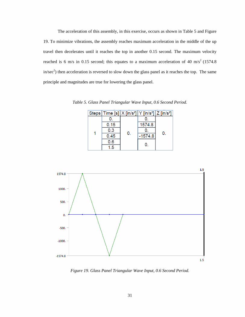
The acceleration of this assembly, in this exercise, occurs as shown in Table 5 and Figure

19. To minimize vibrations, the assembly reaches maximum acceleration in the middle of the up

travel then decelerates until it reaches the top in another 0.15 second. The maximum velocity

reached is 6 m/s in 0.15 second; this equates to a maximum acceleration of 40 m/s2 (1574.8

in/sec2) then acceleration is reversed to slow down the glass panel as it reaches the top. The same

principle and magnitudes are true for lowering the glass panel.

Table 5. Glass Panel Triangular Wave Input, 0.6 Second Period.

Figure 19. Glass Panel Triangular Wave Input, 0.6 Second Period.

32

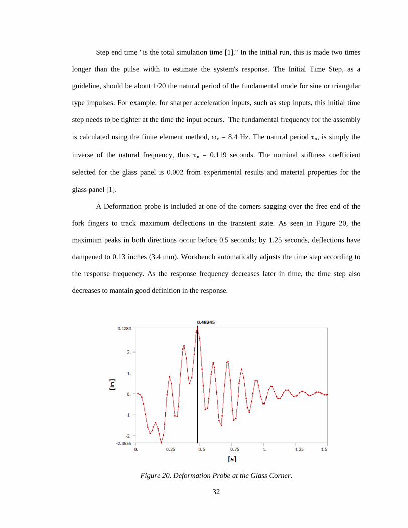
Step end time "is the total simulation time [1]." In the initial run, this is made two times

longer than the pulse width to estimate the system's response. The Initial Time Step, as a

guideline, should be about 1/20 the natural period of the fundamental mode for sine or triangular

type impulses. For example, for sharper acceleration inputs, such as step inputs, this initial time

step needs to be tighter at the time the input occurs. The fundamental frequency for the assembly

is calculated using the finite element method, ωn = 8.4 Hz. The natural period τn, is simply the

inverse of the natural frequency, thus τn = 0.119 seconds. The nominal stiffness coefficient

selected for the glass panel is 0.002 from experimental results and material properties for the

glass panel [1].

A Deformation probe is included at one of the corners sagging over the free end of the

fork fingers to track maximum deflections in the transient state. As seen in Figure 20, the

maximum peaks in both directions occur before 0.5 seconds; by 1.25 seconds, deflections have

dampened to 0.13 inches (3.4 mm). Workbench automatically adjusts the time step according to

the response frequency. As the response frequency decreases later in time, the time step also

decreases to mantain good definition in the response.

Figure 20. Deformation Probe at the Glass Corner.

33

4.1.1 Variation of the Pulse Width Sensitivity Study

This is the first study conducted on the sensitivity of varying the pulse width of the

acceleration input and tracking variations in tip deflections and stresses. An important parameter

to define is the time to maximum acceleration (TMA); this is the time it takes for the input to

reach its maximum value. In the case of a half sine acceleration input for example, the TMA

would be half of the pulse width. The convergence trend seen in this dynamic case settles when

the time to maximum acceleration (TMA) of the input is at least twice the natural period of the

glass panel. Table 6 and Figure 21 show that maximum tip deflection reaches a value of

approximately 2.0 inches for TMA ratios of 1.9 and higher. For values where this TMA ratio falls

below 1.9, it defines progressively sharper shocks where deflections start to increase rapidly.

Depending on the specific type of glass, it would most likely break before being able to sustain a

shock with a TMA ratio of 0.3 where deflections are calculated above 10 inches. Asuming it does

not, and that deformations are linear, Table 6 and Figure 21 describe maximum amplitude of

vibration as a function of different pulse widths or TMA ratios.

Table 6. Glass Panel Stress and Deflection Sensitivity to Impulse Duration.

2.2 m X 2.5 m Glass Panel Dynamic Analysis Results. All Runs Used the Same Mesh and a Stiffness Coefficient of 0.002. Natural Period is calculated at 0.119 seconds for the Fundamental

Mode of the Glass Structured Restrained by the Steel Fork. Time to

Maximum Acceleration

(s)

Ratio of Time to Maximum

Acceleration / Natural Period

Total Input Duration -

Triangular Pulse (s)

Maximum Tip Deflection -

Vertical Probe (in)

Maximum Equivalent Stress on Glass Surface

at Free End of Fork (ksi)

0.015 0.1 0.06 6.09 17.79

0.023 0.2 0.09 9.66 28.32

0.038 0.3 0.15 10.26 31.16

0.075 0.6 0.3 4.93 14.29

0.150 1.3 0.6 3.13 6.74 0.225 1.9 0.9 2.13 4.06 0.300 2.5 1.2 1.96 4.14 0.375 3.2 1.5 2.04 3.59

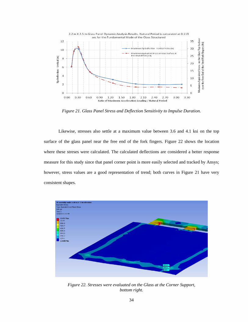
34

Figure 21. Glass Panel Stress and Deflection Sensitivity to Impulse Duration.

Likewise, stresses also settle at a maximum value between 3.6 and 4.1 ksi on the top

surface of the glass panel near the free end of the fork fingers. Figure 22 shows the location

where these streses were calculated. The calculated deflections are considered a better response

measure for this study since that panel corner point is more easily selected and tracked by Ansys;

however, stress values are a good representation of trend; both curves in Figure 21 have very

consistent shapes.

Figure 22. Stresses were evaluated on the Glass at the Corner Support, bottom right.

35

4.1.2 Transient Analysis vs Static Analysis

Transient analyses, methods A and B in Table 7, are more involved than static analyses;

engineers often simplify transient cases as static cases for different reasons. Static models are

often used to analyze dynamic systems and their results may not be correct in many cases. Table

7 includes two static analyses, cases D, and E, that are sometimes used to calculate maximum

stresses and deflection of dynamic systems; in case E, the resultant force from the weight of the

part multiplied with the g value of the acceleration is used and simply exerted on the body; or

similarly, in case D, the density of the part is modified so the part weight is representative to what

it would be due to a higher value of acceleration. Case C involves using acceleration over a long

period of time such as 1 second which does not produce a transient response on the system and a

quasistatic result is obtained.

Something worth noting in Table 7 is that stresses and deflections in case C are the

stresses and deflections one would expect from a transient analysis, as the pulse width of the

input increases to a large value above 0.45 seconds, corresponding to the total input duration of

0.9 seconds in Table 6.

In Table 7, stresses and deflections in Static Cases D and E are shown to be over 3.5X

and over 4X lower respectively, when compared to transient analysis Case A. Discrepancies in

results can be even more significant when compared with sharper shock inputs such as those with

TMA ratios less than 0.6 in Table 6. This is a significant difference, thus running static analyses

in place of transient analyses for mechanical evaluation of impulse loading is not considered

appropiate. Furthermore, two inputs with the same pulse width but different magnitudes can

excite the part differently. This energy content of the input is another parameter that can influence

the structural response which would only be evident from a transient analysis.

36

Table 7. Transient Cases A, B, C vs Static Cases D and E.

Case Description

Max Stress on Glass Surface

over the Free End of the Fork

Fingers (ksi)

Max Vertical Deflection At Glass Corner

(in)

A Glass under 4.1 g acceleration, & 0.3 second total triangular input 14.29 4.93

B Glass under 4.1 g acceleration, & 0.6 second total triangular input 6.74 3.13

C Glass under 4.1g acceleration, ramped in 1 second 3.85 1.95

D Static Case - Glass with 4X density for 4X the weight 3.81 1.36

E Static Case - Glass with 4X force equivalent to 4X the weight 3.84 1.17

4.2 Second Case Study: The I508 Inlet Guide Vane Housing (IGV)

The I508 IGV is the subject in this second case study and it has material callouts for

6061-T6 aluminum. Material specifications used in these analyses are as follows: density is 0.098

lbf/in3, modulus of elasticity is 10E6 psi, and Poisson's ratio is 0.33. The acceleration input used

for this analysis is crash hazard shock involving a half sine 40 g magnitude impulse with a 11 ms

pulse width as shown in Figure 23.

Figure 23. A Crash Hazard Shock, a Half Sine Pulse with 40 g in 11 milliseconds.

37

4.2.1 IGV Stresses and Deflections vs Direction of Shock

Using a simplified IGV model with a reduced number of vanes, a 40 g impulse load is

applied in all three cartesian axes independently to determine which axis has the weakest

response to this input. This model with over 90x103 elements and run times of several hours

provides useful preliminary results as presented in Table 8. For boundary conditions, a fixed

support is placed on the flange of this structure.

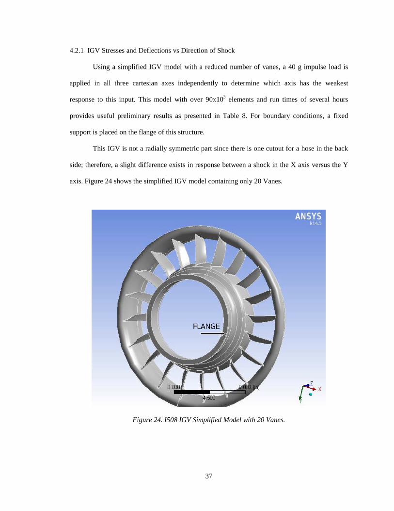
This IGV is not a radially symmetric part since there is one cutout for a hose in the back

side; therefore, a slight difference exists in response between a shock in the X axis versus the Y

axis. Figure 24 shows the simplified IGV model containing only 20 Vanes.

Figure 24. I508 IGV Simplified Model with 20 Vanes.

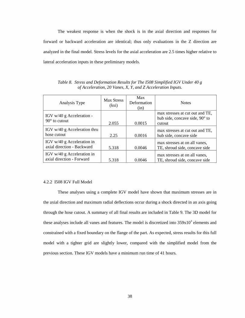
38

The weakest response is when the shock is in the axial direction and responses for

forward or backward acceleration are identical; thus only evaluations in the Z direction are

analyzed in the final model. Stress levels for the axial acceleration are 2.5 times higher relative to

lateral acceleration inputs in these preliminary models.

Table 8. Stress and Deformation Results for The I508 Simplified IGV Under 40 g of Acceleration, 20 Vanes, X, Y, and Z Acceleration Inputs.

Analysis Type Max Stress (ksi)

Max Deformation

(in) Notes

IGV w/40 g Acceleration - 90° to cutout 2.055 0.0015

max stresses at cut out and TE, hub side, concave side, 90° to cutout

IGV w/40 g Acceleration thru hose cutout 2.25 0.0016

max stresses at cut out and TE, hub side, concave side

IGV w/40 g Acceleration in axial direction - Backward 5.318 0.0046

max stresses at on all vanes, TE, shroud side, concave side

IGV w/40 g Acceleration in axial direction - Forward 5.318 0.0046

max stresses at on all vanes, TE, shroud side, concave side

4.2.2 I508 IGV Full Model

These analyses using a complete IGV model have shown that maximum stresses are in

the axial direction and maximum radial deflections occur during a shock directed in an axis going

through the hose cutout. A summary of all final results are included in Table 9. The 3D model for

these analyses include all vanes and features. The model is discretized into 359x103 elements and

constrained with a fixed boundary on the flange of the part. As expected, stress results for this full

model with a tighter grid are slightly lower, compared with the simplified model from the

previous section. These IGV models have a minimum run time of 41 hours.

39

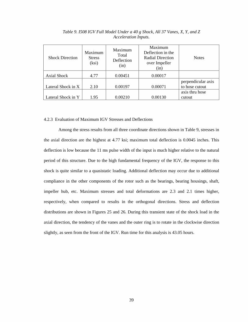
Table 9. I508 IGV Full Model Under a 40 g Shock, All 37 Vanes, X, Y, and Z Acceleration Inputs.

Shock Direction Maximum

Stress (ksi)

Maximum Total

Deflection (in)

Maximum Deflection in the Radial Direction

over Impeller (in)

Notes

Axial Shock 4.77 0.00451 0.00017

Lateral Shock in X 2.10 0.00197 0.00071 perpendicular axis to hose cutout

Lateral Shock in Y 1.95 0.00210 0.00130 axis thru hose cutout

4.2.3 Evaluation of Maximum IGV Stresses and Deflections

Among the stress results from all three coordinate directions shown in Table 9, stresses in

the axial direction are the highest at 4.77 ksi; maximum total deflection is 0.0045 inches. This

deflection is low because the 11 ms pulse width of the input is much higher relative to the natural

period of this structure. Due to the high fundamental frequency of the IGV, the response to this

shock is quite similar to a quasistatic loading. Additional deflection may occur due to additional

compliance in the other components of the rotor such as the bearings, bearing housings, shaft,

impeller hub, etc. Maximum stresses and total deformations are 2.3 and 2.1 times higher,

respectively, when compared to results in the orthogonal directions. Stress and deflection

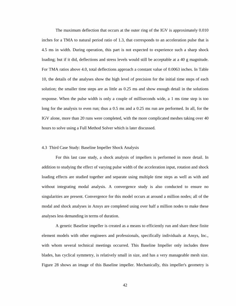
distributions are shown in Figures 25 and 26. During this transient state of the shock load in the

axial direction, the tendency of the vanes and the outer ring is to rotate in the clockwise direction

slightly, as seen from the front of the IGV. Run time for this analysis is 43.05 hours.

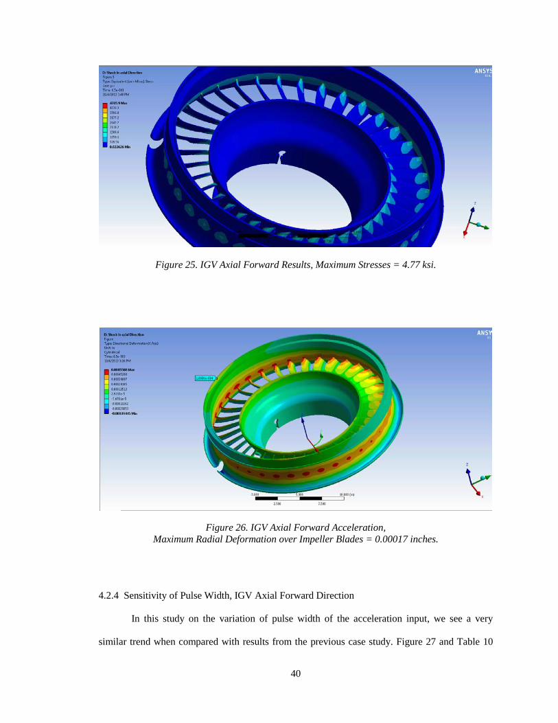
40

Figure 25. IGV Axial Forward Results, Maximum Stresses = 4.77 ksi.

Figure 26. IGV Axial Forward Acceleration, Maximum Radial Deformation over Impeller Blades = 0.00017 inches.

4.2.4 Sensitivity of Pulse Width, IGV Axial Forward Direction

In this study on the variation of pulse width of the acceleration input, we see a very

similar trend when compared with results from the previous case study. Figure 27 and Table 10

41

show that in the case of this IGV, deflections (solid curve) and stresses (dashed curve) start

increasing rapidly for a TMA/Natural-Period ratio of approximately 3.5 and under; in the

previous case with the glass panel this ratio was closer to 2.

Figure 27. Simplified IGV Stress and Deflection Sensitivity to Impulse Duration, 40 g Forward Shock, τn = 1.7 ms.

Table 10. High Resolution Results For the Dynamic Response of a Simplified IGV to a 40 g Axial Forward Acceleration.

Pulse Width (ms)

Time to Maximum

Acceleration, TMA (ms)

Ratio TMA / Natural Period

Maximum Stress (ksi)

Maximum Total

Deflection (in)

Details

1.0 0.50 0.3 8.998 0.0051 0.25 ms ITS 3.0 1.50 0.9 10.155 0.0096 0.25 ms ITS 4.5 2.25 1.3 10.686 0.0098 0.5 ms ITS 6.0 3.00 1.7 11.140 0.0092 0.5 ms ITS 6.5 3.25 1.9 11.040 0.0091 0.5 ms ITS

11.0 5.50 3.2 8.877 0.0068 same results at 1ms ITS and 0.5ms ITS

22.0 11.00 6.4 8.390 0.0063 0.5 ms ITS 44.0 22.00 12.7 8.550 0.0063 0.5 ms ITS

42

The maximum deflection that occurs at the outer ring of the IGV is approximately 0.010

inches for a TMA to natural period ratio of 1.3, that corresponds to an acceleration pulse that is

4.5 ms in width. During operation, this part is not expected to experience such a sharp shock

loading; but if it did, deflections and stress levels would still be acceptable at a 40 g magnitude.

For TMA ratios above 4.0, total deflections approach a constant value of 0.0063 inches. In Table

10, the details of the analyses show the high level of precision for the initial time steps of each

solution; the smaller time steps are as little as 0.25 ms and show enough detail in the solutions

response. When the pulse width is only a couple of milliseconds wide, a 1 ms time step is too

long for the analysis to even run; thus a 0.5 ms and a 0.25 ms run are performed. In all, for the

IGV alone, more than 20 runs were completed, with the more complicated meshes taking over 40

hours to solve using a Full Method Solver which is later discussed.

4.3 Third Case Study: Baseline Impeller Shock Analysis

For this last case study, a shock analysis of impellers is performed in more detail. In

addition to studying the effect of varying pulse width of the acceleration input, rotation and shock

loading effects are studied together and separate using multiple time steps as well as with and

without integrating modal analysis. A convergence study is also conducted to ensure no

singularities are present. Convergence for this model occurs at around a million nodes; all of the

modal and shock analyses in Ansys are completed using over half a million nodes to make these

analyses less demanding in terms of duration.

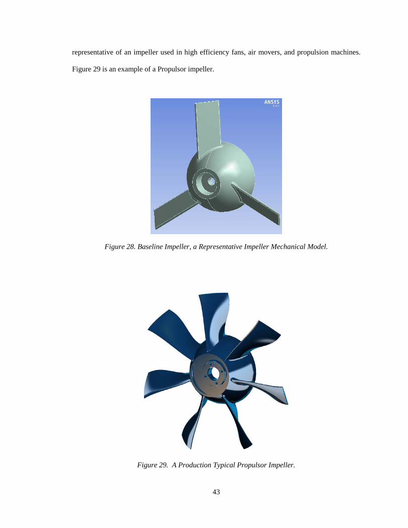
A genetic Baseline impeller is created as a means to efficiently run and share these finite

element models with other engineers and professionals, specifically individuals at Ansys, Inc.,

with whom several technical meetings occurred. This Baseline Impeller only includes three

blades, has cyclical symmetry, is relatively small in size, and has a very manageable mesh size.

Figure 28 shows an image of this Baseline impeller. Mechanically, this impeller's geometry is

43

representative of an impeller used in high efficiency fans, air movers, and propulsion machines.

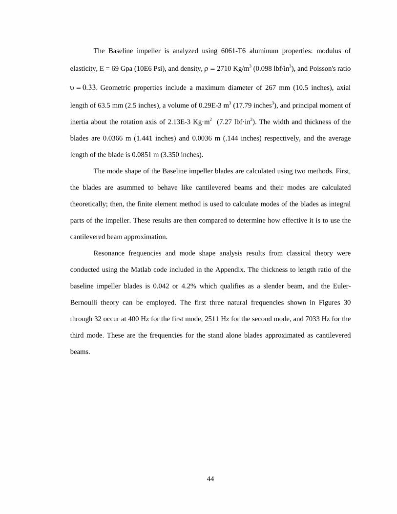
Figure 29 is an example of a Propulsor impeller.

Figure 28. Baseline Impeller, a Representative Impeller Mechanical Model.

Figure 29. A Production Typical Propulsor Impeller.

44

The Baseline impeller is analyzed using 6061-T6 aluminum properties: modulus of

elasticity, E = 69 Gpa (10E6 Psi), and density, ρ = 2710 Kg/m3 (0.098 lbf/in3), and Poisson's ratio

υ = 0.33. Geometric properties include a maximum diameter of 267 mm (10.5 inches), axial

length of 63.5 mm (2.5 inches), a volume of 0.29E-3 m3 (17.79 inches3), and principal moment of

inertia about the rotation axis of 2.13E-3 Kg·m2 (7.27 lbf·in2). The width and thickness of the

blades are 0.0366 m (1.441 inches) and 0.0036 m (.144 inches) respectively, and the average

length of the blade is 0.0851 m (3.350 inches).

The mode shape of the Baseline impeller blades are calculated using two methods. First,

the blades are asummed to behave like cantilevered beams and their modes are calculated

theoretically; then, the finite element method is used to calculate modes of the blades as integral

parts of the impeller. These results are then compared to determine how effective it is to use the

cantilevered beam approximation.

Resonance frequencies and mode shape analysis results from classical theory were

conducted using the Matlab code included in the Appendix. The thickness to length ratio of the

baseline impeller blades is 0.042 or 4.2% which qualifies as a slender beam, and the Euler-

Bernoulli theory can be employed. The first three natural frequencies shown in Figures 30

through 32 occur at 400 Hz for the first mode, 2511 Hz for the second mode, and 7033 Hz for the

third mode. These are the frequencies for the stand alone blades approximated as cantilevered

beams.

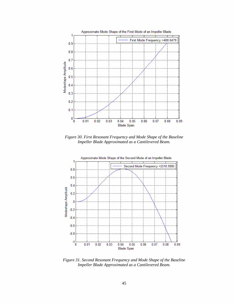
45

Figure 30. First Resonant Frequency and Mode Shape of the Baseline Impeller Blade Approximated as a Cantilevered Beam.

Figure 31. Second Resonant Frequency and Mode Shape of the Baseline Impeller Blade Approximated as a Cantilevered Beam.

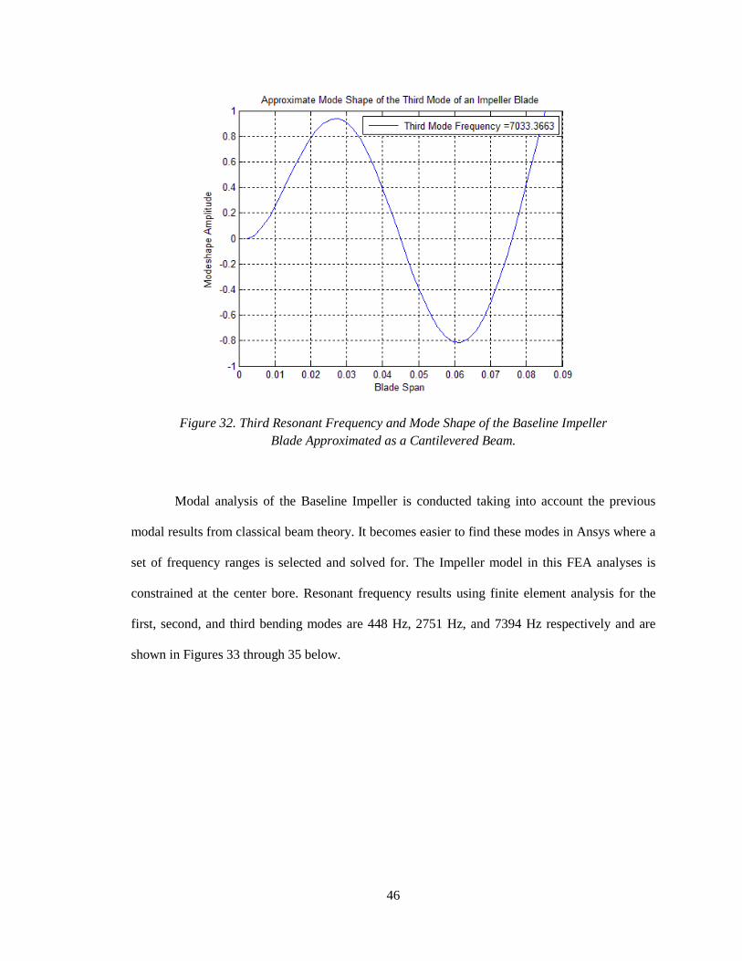
46

Figure 32. Third Resonant Frequency and Mode Shape of the Baseline Impeller Blade Approximated as a Cantilevered Beam.

Modal analysis of the Baseline Impeller is conducted taking into account the previous

modal results from classical beam theory. It becomes easier to find these modes in Ansys where a

set of frequency ranges is selected and solved for. The Impeller model in this FEA analyses is

constrained at the center bore. Resonant frequency results using finite element analysis for the

first, second, and third bending modes are 448 Hz, 2751 Hz, and 7394 Hz respectively and are

shown in Figures 33 through 35 below.

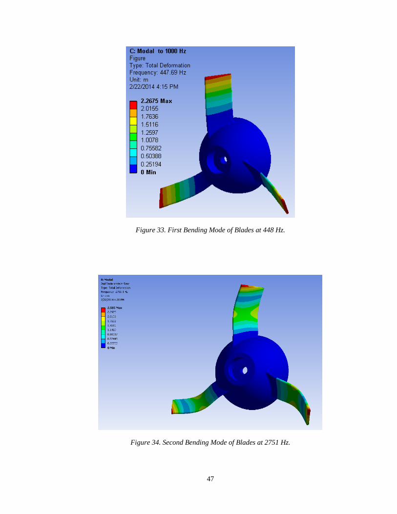
47

Figure 33. First Bending Mode of Blades at 448 Hz.

Figure 34. Second Bending Mode of Blades at 2751 Hz.

48

Figure 35. Third Bending Mode of Blades at 7394 Hz.

Performing an initial modal analysis using Matlab and the Euler-Bernoulli beam theory

has proven to be very useful and a very efficient preliminary analysis that can be performed on

impeller modal analysis prior to a more demanding finite element analysis. Furthermore, Table 11

shows that at least for the first three bending moments, the analytical results are in the range of

10.5% effectiveness or better. Analytical results can be combined with a Campbell diagram as a

preliminary design step towards designing an impeller clear of blade resonances at specific

operating points in the system. Next, Ansys is used for shock analysis of this Baseline impeller

model.

Table 11. Analytical and FEA Modal Results For The Baseline Impeller.

Bending Modes

Analytical Result of Bending Modes of

Blades as Cantilevered Beams (Hz)

FEA Blade Bending Mode of Baseline Bladed Impeller

(Hz)

Difference Of Analytical Results Relative to FEA

Results (%) 1st 400.7 447.7 10.5% 2nd 2511.2 2751.1 8.7% 3rd 7033.4 7394.4 4.9%

49

4.3.1 Baseline Impeller Shock Analysis By Finite Element Analysis

Shock analysis is studied in depth using the Baseline Impeller model shown in Figure 28.

Primarily, this model is designed to study the effects of rotation and shock; these loading types

are studied together and independently, as well as in combination with modal analysis which is

called Mode Superposition analysis. Secondly, this model is also used to study once again the

effect of varying the pulse width of an acceleration shock input and compare with the other

systems studied earlier. A half-sine acceleration input of 50 g in Figure 36 shows a graph of this

input generated in an Excel worksheet. This becomes the tabular input used in Ansys for a

transient analysis.

Figure 36. Half Sine Acceleration Shock Input with a Positive Magnitude of 50 g and a Pulse Width of 5 ms.

The Baseline Impeller 3D model is meshed using tetrahedron elements with a higher

element count where the geometry has more abrupt transitions and where the highest strain is

expected. This mesh is controlled mainly by minimum number elements across any thickness of

the part and by curvature in the geometry. The normal angle is set to 45°, minimum number of

cells is set to 2, and transition between fine and coarse areas in the model is set to slow for higher

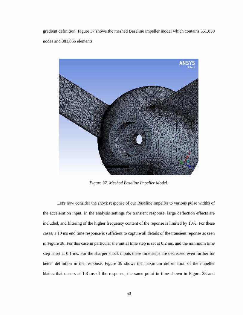
50

gradient definition. Figure 37 shows the meshed Baseline impeller model which contains 551,830

nodes and 381,866 elements.

Figure 37. Meshed Baseline Impeller Model.

Let's now consider the shock response of our Baseline Impeller to various pulse widths of

the acceleration input. In the analysis settings for transient response, large deflection effects are

included, and filtering of the higher frequency content of the reponse is limited by 10%. For these

cases, a 10 ms end time response is sufficient to capture all details of the transient reponse as seen

in Figure 38. For this case in particular the initial time step is set at 0.2 ms, and the minimum time

step is set at 0.1 ms. For the sharper shock inputs these time steps are decreased even further for

better definition in the response. Figure 39 shows the maximum deformation of the impeller

blades that occurs at 1.8 ms of the response, the same point in time shown in Figure 38 and

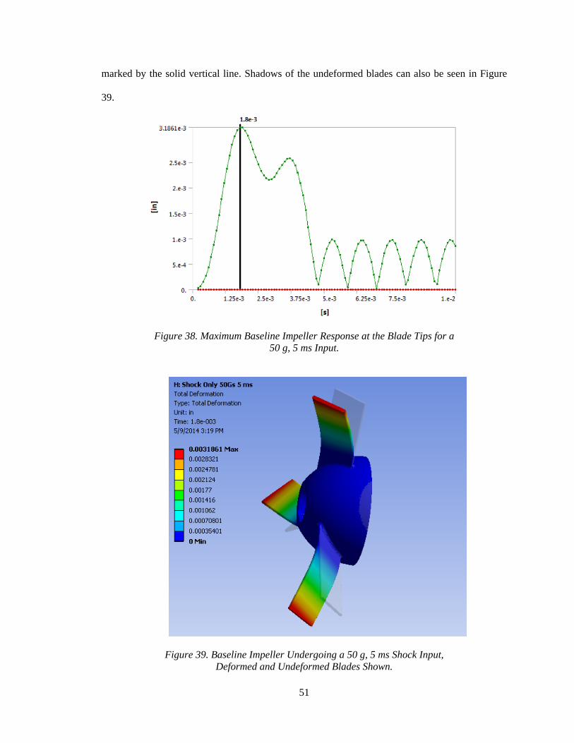
51

marked by the solid vertical line. Shadows of the undeformed blades can also be seen in Figure

39.

Figure 38. Maximum Baseline Impeller Response at the Blade Tips for a 50 g, 5 ms Input.

Figure 39. Baseline Impeller Undergoing a 50 g, 5 ms Shock Input, Deformed and Undeformed Blades Shown.

52

In this third and last study of effects of pulse width variations, the trend is similar to the

previous systems. It has a peak, then gradually decreases until it converges to a minimum value

for deformation and stress. Maximum values for total deformation always occur at the blade tips.

For this case study we continue to track and compare deformation values as opposed to stress

values which are included for reference only.

Figure 40. Baseline Impeller Sensitivity to Pulse Width, 50 g Shock, τn = 2.2 ms.

In this particular case, maximum total deflection of the impeller blade tips occurs during

an acceleration pulse width of 2 ms, which corresponds to a TMA/Natural-Period Ratio of 0.45;

for reference, the maximum total deflection at this point is 0.0047 inches as shown in Figure 40

and Table 12. Similarly, and from a separate study by J. Luo, et. al on a head actuator assembly

subjected to the same type of input, the highest amplitude for the transient response occurs when

pulse frequency is 0.66 of the natural frequency [15].

53

Maximum total deformation and stress values start to increase when this ratio is under

1.00. This Baseline Impeller was not designed to operate inside a real machine, but it does have

representative mechanical characteristics as those from a real impeller in production; deformation

and stress values are for relative comparison purposes but they are low when compared to the

strength of 6061-T6 aluminum.

Table 12. Table of Values for Figure 41.

Pulse Width (ms)

Time to Maximum Input Acceleration

(ms)

TMA/ Natural-Period

Ratio

Max Stresses

(psi)

Total Deformation

(in)

1.0 0.50 0.22 1148 0.00397 1.5 0.75 0.34 1430 0.00467 2.0 1.00 0.45 1499 0.00473 2.5 1.25 0.56 1455 0.00453 4.0 2.00 0.90 1236 0.00368 5.0 2.50 1.12 1074 0.00319 7.0 3.50 1.57 1085 0.00317 11.0 5.50 2.46 1017 0.00293

4.3.2 Baseline Impeller Undergoing Rotation and Shock, Two Solution Methods

Properly analyzing an impeller subjected to a single shock input while undergoing

rotation at the same time is often essential in the design of rotating machinery and it is discussed

next. Two solution methods from Ansys are presented: using the Full Method to solve for the

transient response and the Mode Superposition Method (Superposition) which involves using a

combination of static, modal, and transient analysis. The latter method may not require a static

analysis; however, in this case it is used for calculating deformation and stress due to centrifugal

forces from rotation.

Large deflection and stiffening effects due to rotation are accounted for; otherwise, for

the Baseline impeller in particular, deformations would be 19.4% higher. Time integration effects

54

are also included. This is important in transient analysis where transient effects such as structural

inertia are taken into account where solutions at every time step are based on a previous solution.

With Time Integration turned off, the system response is zero after the time dependent loading

has ended. Next, let's compare differences and similarities between the Full Method and the

Mode Superposition Method.

The Full Method uses the full system matrices to calculate the transient response (no

matrix reduction). It is the more general method because it allows all types of nonlinearities to be

included (plasticity, large deflections, large strain, and so on) [14]. The main disadvantage of

using this method is that it takes a considerable amount of time and computer resources to solve,

relative to the Mode Superposition Method; it could take many hours or several days, whereas the

latter method could takes a matter of minutes. Per the Ansys Mechanical APDL Structural

Analysis Guide, advantages of the Full Method are:

It is easier to use because you do not have to worry about choosing mode shapes.

It allows all types of nonlinearities.

It uses full matrices, so no mass matrix approximation is involved.

All displacements and stresses are calculated in a single pass.

It accepts all types of loads: nodal forces, imposed (nonzero) displacements (although not

recommended), and element loads (pressures and temperatures) and allows tabular

boundary condition specification via TABLE type array parameters.

It allows effective use of solid-model loads.

The Full Method solution is used on the Baseline Impeller to solve for the transient

response. In the set up of this model, the impeller is simply fixed at the center bore for simplicity;

the loading conditions imposed include a counterclockwise rotation of 10,000 RPM and an axial

impulse of 50 g with a 5 ms pulse width; the shape of the impulse is a half-sine wave as shown in

Figure 36. The acceleration of 0 g shown in Figure 41 is the acceleration for one of the other axes

55

which is in fact zero. In this kind of analyses, a fixed support or a frictionless support show

equivalent results. In calculation of stresses and deflections due to rotation, the code simply

applies the centrifugal force to all the nodes with degrees of freedom in the radial direction; a

fixed support is used in this case. These loading and support conditions will be the same as used

in the Mode Superposition Method.

Figure 41. Initial Conditions for the Baseline Impeller Transient Analysis.

Figure 42 shows the location of the probe at the corner of the leading edge of the impeller

blade tip. Tracking results at this location is helpful since it provides a discrete reference point for

comparing deformation results between our two solver solutions.

56

Figure 42. Probe Location for Axial Deformation Calculations.

Rotation causes deflections of the blades in the negative Y directions or rearward axial

direction. The shock is in the negative Y so the response to the shock is in the positive Y

direction; this impulse reaches a peak at 10.5 ms and it is approximately at this time that the

maximum deflection is influenced by the shock response as seen in Figure 43. Deflections due to

rotation and shock act in opposite directions. The response from the shock input is not large; in

this case study, our only concern is the accuracy of the response and process. Also, for sake of

comparison, only axial deflections are studied since these are a better point of reference relative

to stress values, which may change locations depending on the sharpness of the shock.

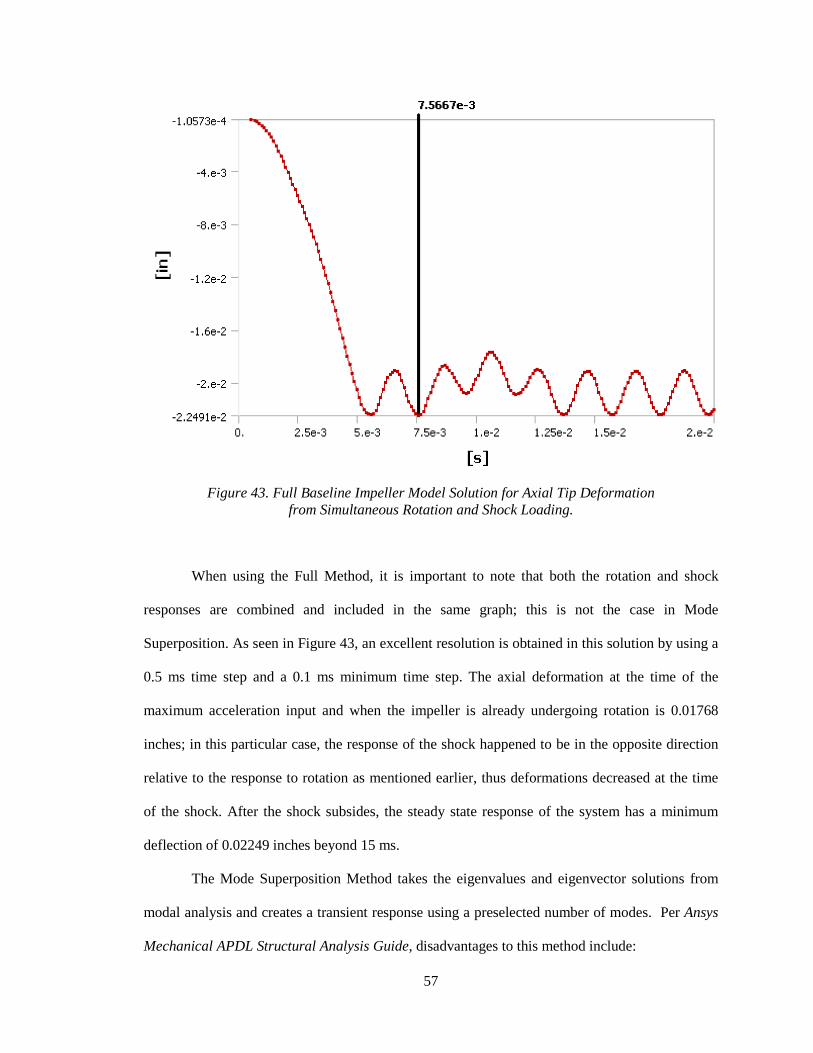
57

Figure 43. Full Baseline Impeller Model Solution for Axial Tip Deformation from Simultaneous Rotation and Shock Loading.

When using the Full Method, it is important to note that both the rotation and shock

responses are combined and included in the same graph; this is not the case in Mode

Superposition. As seen in Figure 43, an excellent resolution is obtained in this solution by using a

0.5 ms time step and a 0.1 ms minimum time step. The axial deformation at the time of the

maximum acceleration input and when the impeller is already undergoing rotation is 0.01768

inches; in this particular case, the response of the shock happened to be in the opposite direction

relative to the response to rotation as mentioned earlier, thus deformations decreased at the time

of the shock. After the shock subsides, the steady state response of the system has a minimum

deflection of 0.02249 inches beyond 15 ms.

The Mode Superposition Method takes the eigenvalues and eigenvector solutions from

modal analysis and creates a transient response using a preselected number of modes. Per Ansys

Mechanical APDL Structural Analysis Guide, disadvantages to this method include:

58

• The time step must remain constant throughout the transient, so automatic time stepping

is not allowed.

• The only nonlinearity allowed is simple node-to-node contact (gap condition).

• It does not accept imposed (nonzero) displacements.

Some advantages are:

• It is faster and less expensive than the Full Method for many problems.

• Element loads applied in the preceding modal analysis can be applied in the transient

dynamic analysis via the LVSCALE command.

• It accepts modal damping (damping ratio as a function of mode number).

The Mode Superposition Method is also used to solve the transient response of the

Baseline Impeller undergoing the same loading and same support type from the Full Method

discussed previously. When running this method, a similar solution is obtained relative to the Full

Method yet it only takes a fraction of the time to solve. The main difference is that in the Mode

Superposition Method, the analysis is broken down in several parts. In this case, three separate

analyses were integrated: static, modal, and transient analyses. These separate analyses are

performed in that order. Once solutions for the different systems are obtained, the total

deformation values for the same locations are added to obtain an overall value. Knowing

individual responses for discrete points and times could be beneficial to help understand which

loading is more critical. The meshed model used is seen in Figure 37. The Ansys Workbench

model used to set up the Mode Superposition analysis of the Baseline Impeller is shown in Figure

44; this model shows how the static solution is the pre-stressed condition for the Modal Analysis,

and this in turn is the initial condition for the transient model where shock loading is carried out.

59

Figure 44. A Mode Superposition Model from Ansys Mechanical.

In the Mode Superposition Method for this case study, we start with static analysis to

determine the effects due to the impeller rotation only. Centrifugal loading due to rotation is

analyzed for a rotation of 10,000 RPM with a fixed support at the center bore, which is equivalent

to a frictionless support. This loading is ramped over a period of 1 second.

Figure 45. Static Analysis Performed as Part of Mode Superposition Method.

The axial deformation solution from the static analysis calculates a maximum axial

deformation of 0.02161 inches at the leading edge tip of the impeller blades; these deflect in the

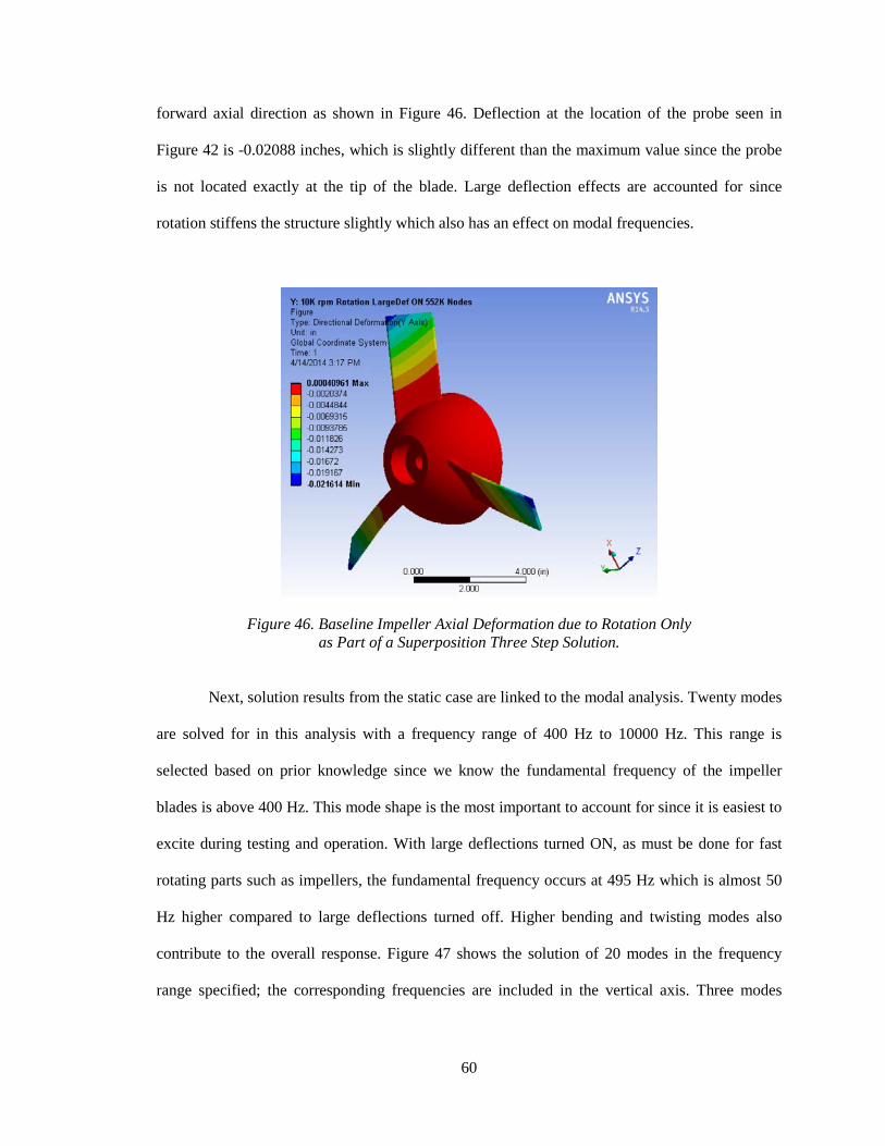
60

forward axial direction as shown in Figure 46. Deflection at the location of the probe seen in

Figure 42 is -0.02088 inches, which is slightly different than the maximum value since the probe

is not located exactly at the tip of the blade. Large deflection effects are accounted for since

rotation stiffens the structure slightly which also has an effect on modal frequencies.

Figure 46. Baseline Impeller Axial Deformation due to Rotation Only as Part of a Superposition Three Step Solution.

Next, solution results from the static case are linked to the modal analysis. Twenty modes

are solved for in this analysis with a frequency range of 400 Hz to 10000 Hz. This range is

selected based on prior knowledge since we know the fundamental frequency of the impeller

blades is above 400 Hz. This mode shape is the most important to account for since it is easiest to

excite during testing and operation. With large deflections turned ON, as must be done for fast

rotating parts such as impellers, the fundamental frequency occurs at 495 Hz which is almost 50

Hz higher compared to large deflections turned off. Higher bending and twisting modes also

contribute to the overall response. Figure 47 shows the solution of 20 modes in the frequency

range specified; the corresponding frequencies are included in the vertical axis. Three modes

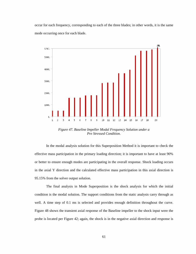
61

occur for each frequency, corresponding to each of the three blades; in other words, it is the same

mode occurring once for each blade.

Figure 47. Baseline Impeller Modal Frequency Solution under a Pre Stressed Condition.

In the modal analysis solution for this Superposition Method it is important to check the

effective mass participation in the primary loading direction; it is important to have at least 90%

or better to ensure enough modes are participating in the overall response. Shock loading occurs

in the axial Y direction and the calculated effective mass participation in this axial direction is

95.15% from the solver output solution.

The final analysis in Mode Superposition is the shock analysis for which the initial

condition is the modal solution. The support conditions from the static analysis carry through as

well. A time step of 0.1 ms is selected and provides enough definition throughout the curve.

Figure 48 shows the transient axial response of the Baseline impeller to the shock input were the

probe is located per Figure 42; again, the shock is in the negative axial direction and response is

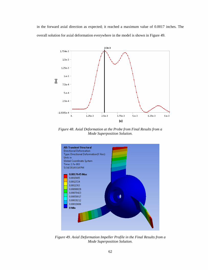
62

in the forward axial direction as expected; it reached a maximum value of 0.0017 inches. The

overall solution for axial deformation everywhere in the model is shown in Figure 49.

Figure 48. Axial Deformation at the Probe from Final Results from a Mode Superposition Solution.

Figure 49. Axial Deformation Impeller Profile in the Final Results from a Mode Superposition Solution.

63

Adding the values for axial deformation, obtained from the Mode Superposition Method,

at the location of the probe due to rotation and shock at 2.7 ms equates to:

- 0.02088 + 0.001754 = -0.0191 inches

The corresponding value obtained using the Full Transient Method is -0.01768 inches;

the difference in results between both methods is only 0.0014 inches for this case study.

In conclusion, the Mode Superposition Method helps tremendously with quickly

evaluating changes in the 3D model and fine tuning the design; additionally, it leaves enough

computer resources available to do other engineering tasks. A computer running a Full Method

solver would most likely use most of the computer memory and processor power available. A

Superposition Method solution allows more visibility into deformation and stress effects caused

by each loading condition; changes on these loading conditions can be easily studied

independently. The Full Method solution is ideal when there is little time to set up a model and

when a solution is not needed right away.

4.3.3 Summary of Chapter 4

Three case studies were completed in Chapter 4: Glass Panel Undergoing a 4 g

Acceleration, The I508 IGV, and Baseline Impeller Shock Analysis. An important comparison

was made between two different methods available for solving shock analyses: the Full Method

and Mode Superposition Method. Many sensitivity studies related to shock analysis were

conducted including using static analysis as a substitute for shock analysis, analytical modal

analysis of impeller blades modeled as cantilevered beams, and effects of varying acceleration

pulse widths from acceleration inputs.

The study of using static analysis in place of transient analysis for evaluation of shock

concluded that differences in results could be significant if the maximum input loading duration is

similar or less than the natural period of the structure. Furthermore, the energy content of the

input is another parameter that can influence the structural response which would only be evident

64

from a transient analysis. In the theoretical modal analysis of impeller blades modeled as beams,

results showed that the mode frequencies of the first three modes were 10.5% or better when

compared with finite element results of the blades modeled as integral parts of the impeller.

Therefore, a quick theoretical modal analysis can be incorporated as a preliminary step in the

initial design process of impellers and their vibration response.

A study of the variation of pulse width of acceleration inputs on different systems was

completed; The Glass Panel and Baseline Impeller test cases showed similar trends, the Inlet

Guide Vane Housing less so. This study shows that the structural response has a large amplitude

when the time to maximum acceleration of the input (TMA) is a fraction of natural period; these

curve peaks can be seen in Figures 21 and 40. When the TMA and the natural period are very

similar, the response of the structure reaches a low amplitude range. The plateaus, which may

become nearly constant, can also be seen in Figures 21 and 40, as well as in Figure 27.

The results from all of these studies must be kept in mind during several phases of the life

of a structure, including during the design phase. When designing parts or systems to withstand

shock, "we will find that structures that deal with shock well are not particularly good with regard

to steady-state excitation and vice versa. Once again, this is a classic case of how we must

carefully consider the different factors of a design, weigh their importance, and then come up

with the best overall design that produces acceptable performance in all relevant categories [10]".

65

CHAPTER 5

EXPERIMENTAL AND ANALYTICAL SHOCK TESTING OF THE

H200 MIXED FLOW FAN

A Mixed Flow Fan is evaluated analytically and experimentally for shock conditions per

Military Standard MIL STD 810. A key focus of mechanical design of rotating machinery is to

maintain tight blade tip clearances while simultaneously avoiding any potential tip rub or impact

against the fan shroud due to impulse loadings or any other operating conditions. The shock

testing required by this military standard describes three different levels of tests in three separate

orthogonal directions as shown in Table 13. These types of shock inputs correspond to road,

gunfire, and ballistic shock levels that military equipment must be able to withstand without

failing to maintain operational capabilities. All major components of the fan assembly are

analyzed according to the shock inputs included in Table 13. FEA results show that the ballistic

shock causes the most deflections; for example, impeller ballistic shocks are 1.9X and 2.4X more

severe in terms of deflections when compared to the gun firing and the road load shock,

respectively. Analyses of all applicable components in the mixed flow machine, for the ballistic

shock only, are discussed in the following sections. The cylindrical coordinate system is often

used in these finite element models; the radial direction is comprised of both the lateral and

vertical directions from the Cartesian coordinate system.

Table 13. MIL STD 810 Shock Requirements Using a Half Sine Input.

Shock Load Type Amplitude (g) Pulse Duration (ms)

Road Load 20 ± 3 11.1 ±1.1

Gunfire 25 ± 5 1.5 ±0.2

Ballistic 50 ± 8 0.5 ±0.1

66

5.1 Analytical Results

The assembly and associated components are analyzed for shock loading using finite

element analyses, theoretical calculations, careful measurements, and manufacturer's tolerance

specifications. A cross section of the fan assembly is shown in Figure 50 and describes the major

components of this machine. Analysis of the assembly is complex, due to point contact of the ball

bearings inside the bearing rings; this analysis is separated into four major parts to mitigate the

complexity: analysis of the impeller-rotor subassembly, the front bearing housing (FBH), the ball

bearings, and the remaining non-rotating structure which includes the fan shroud, in particular,

along with the motor support, diffuser, and mounting bracket. These analyses focus on

determining the maximum potential risk for impeller blade contact against the shroud. In

particular, these analyses focus on deflections that could most likely cause a blade tip strike; two

locations are investigated: axial deflections at the blades trailing edges (TE) at the outside

diameter of the impeller and radial deflection at the blades leading edges (LE) as indicated in

Figure 50.

Figure 50. Cross Section of Mixed Flow Fan Assembly for Illustration Purposes.

67

5.1.1 Impeller and Rotor Subassembly

Analyses of the impeller-rotor include shock loading as well as rotational and

aerodynamic effects. The impeller material is 6061-T6 aluminum and the rotor spindle is 17-4-PH

stainless steel. The configuration of this rotor is an overhung type rotor with significant mass at

the front end; the moments that are induced by a shock in one direction do cause deflection in an

orthogonal direction as well. The boundary conditions of the model include two fixed supports at

both bearing journals of the rotor. The impeller is securely fixed to the rotor by a shrink fit; thus,

this connection is defined as bonded. All shock loads are analyzed in two different directions:

axial and radial. The rotor has radial symmetry; therefore, vertical and lateral shocks are

equivalent to a radial shock.

The Full Method for transient analysis is used for this impeller-rotor subassembly; the

loading conditions in this model include a ballistic shock input, as well as centrifugal and

aerodynamic effects. Fine meshing is driven by a curvature definition of 45°, a maximum element

size of 0.100 inches, and a growth rate of 1.50. In the analysis settings, the solution is divided in

two time steps: a lower definition time step for the static loads and a finer definition second step

for the transient shock load. This allows for a more efficient solution in the shortest amount of

time possible using a Full Method. A time delay is implemented for the ballistic shock input

which starts sometime after the end of the rotation and aerodynamic loading as shown in Figure

51.

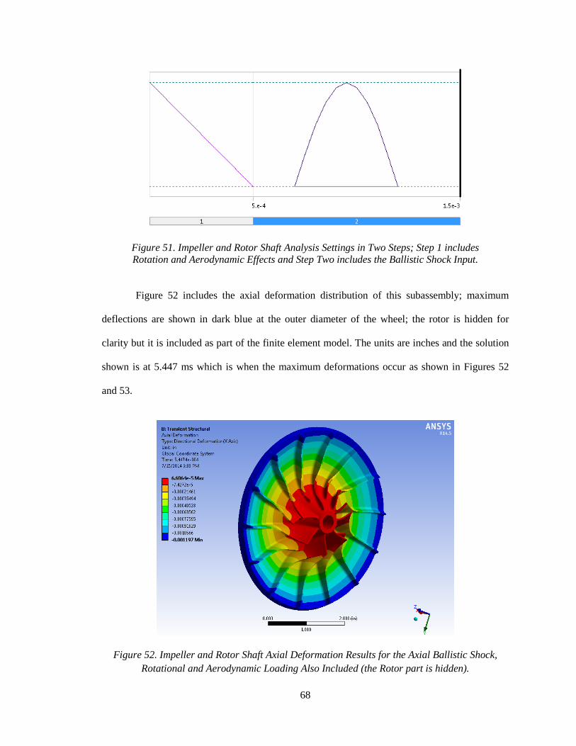
68

Figure 51. Impeller and Rotor Shaft Analysis Settings in Two Steps; Step 1 includes Rotation and Aerodynamic Effects and Step Two includes the Ballistic Shock Input.

Figure 52 includes the axial deformation distribution of this subassembly; maximum

deflections are shown in dark blue at the outer diameter of the wheel; the rotor is hidden for

clarity but it is included as part of the finite element model. The units are inches and the solution

shown is at 5.447 ms which is when the maximum deformations occur as shown in Figures 52

and 53.

Figure 52. Impeller and Rotor Shaft Axial Deformation Results for the Axial Ballistic Shock, Rotational and Aerodynamic Loading Also Included (the Rotor part is hidden).

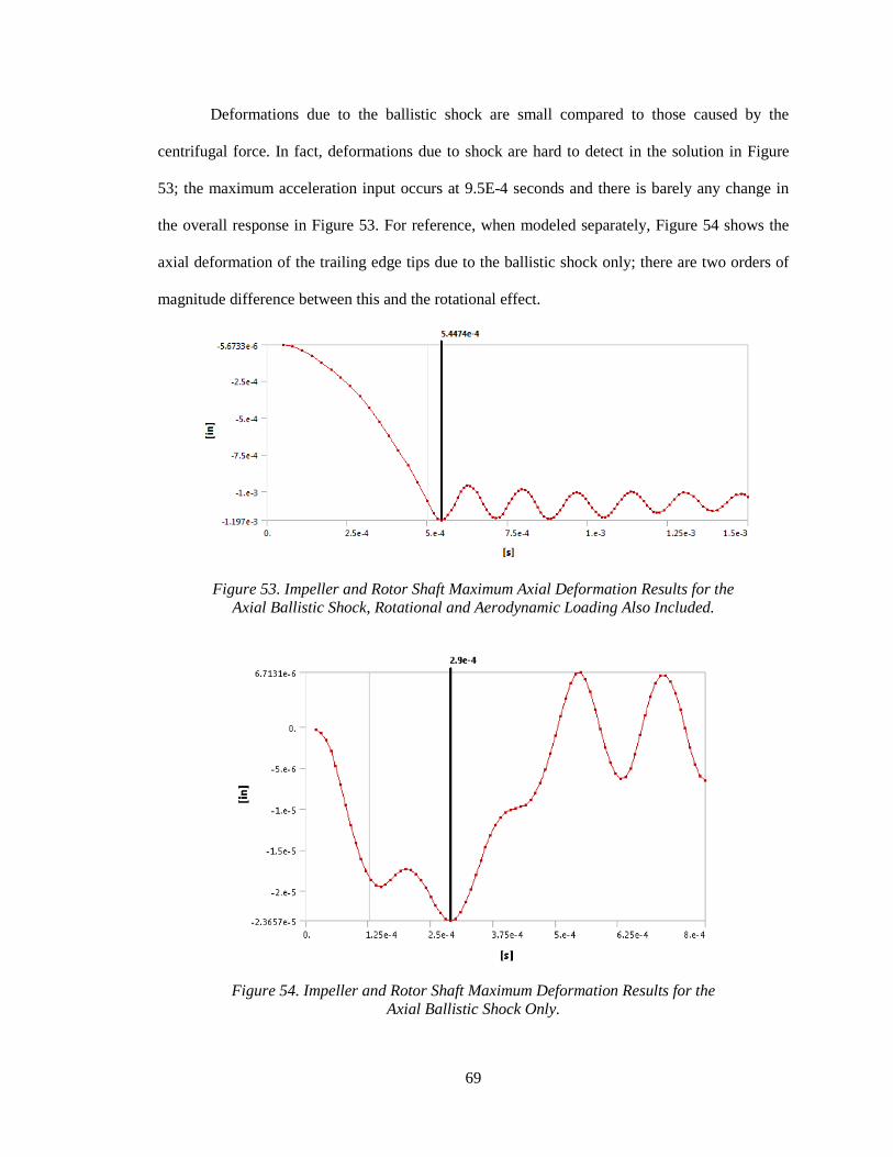
69

Deformations due to the ballistic shock are small compared to those caused by the

centrifugal force. In fact, deformations due to shock are hard to detect in the solution in Figure

53; the maximum acceleration input occurs at 9.5E-4 seconds and there is barely any change in

the overall response in Figure 53. For reference, when modeled separately, Figure 54 shows the

axial deformation of the trailing edge tips due to the ballistic shock only; there are two orders of

magnitude difference between this and the rotational effect.

Figure 53. Impeller and Rotor Shaft Maximum Axial Deformation Results for the Axial Ballistic Shock, Rotational and Aerodynamic Loading Also Included.

Figure 54. Impeller and Rotor Shaft Maximum Deformation Results for the Axial Ballistic Shock Only.

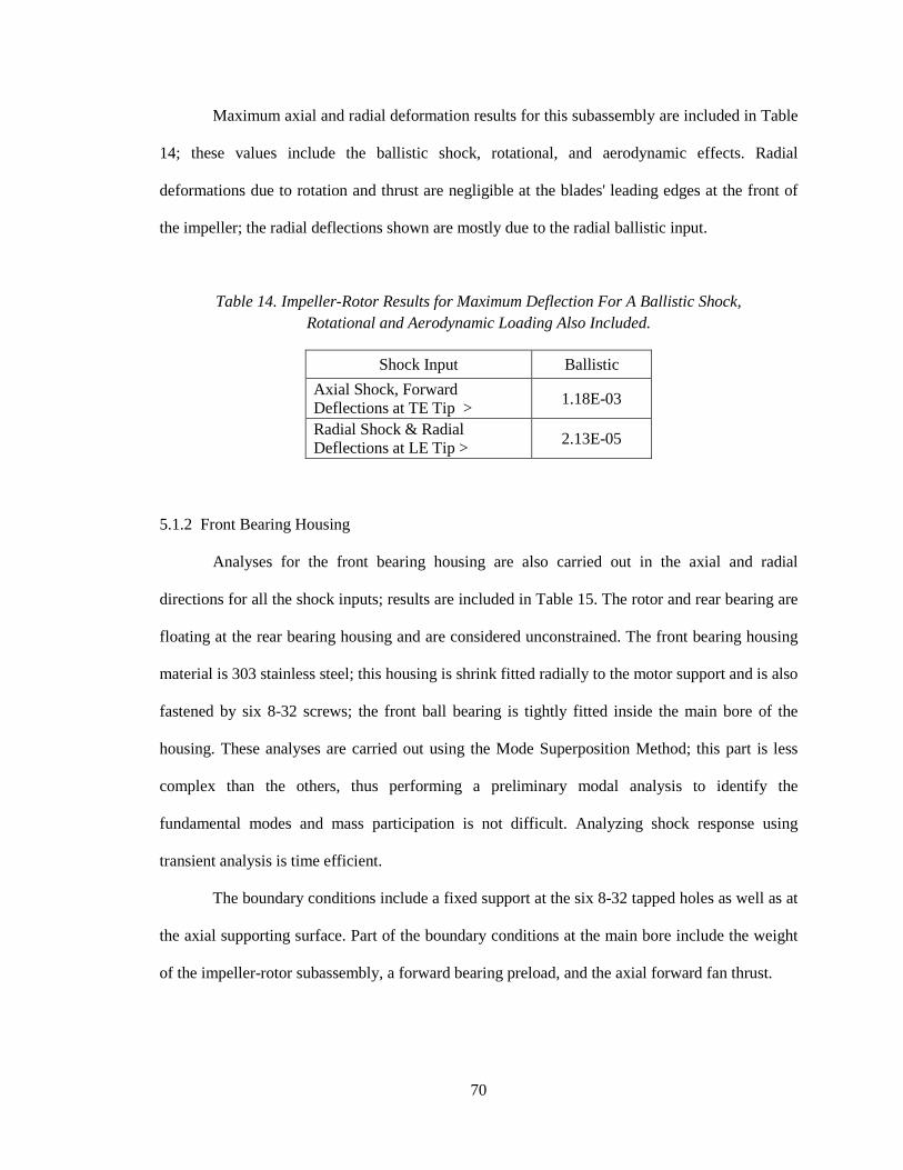
70

Maximum axial and radial deformation results for this subassembly are included in Table

14; these values include the ballistic shock, rotational, and aerodynamic effects. Radial

deformations due to rotation and thrust are negligible at the blades' leading edges at the front of

the impeller; the radial deflections shown are mostly due to the radial ballistic input.

Table 14. Impeller-Rotor Results for Maximum Deflection For A Ballistic Shock, Rotational and Aerodynamic Loading Also Included.

Shock Input Ballistic Axial Shock, Forward Deflections at TE Tip > 1.18E-03

Radial Shock & Radial Deflections at LE Tip > 2.13E-05

5.1.2 Front Bearing Housing

Analyses for the front bearing housing are also carried out in the axial and radial

directions for all the shock inputs; results are included in Table 15. The rotor and rear bearing are

floating at the rear bearing housing and are considered unconstrained. The front bearing housing

material is 303 stainless steel; this housing is shrink fitted radially to the motor support and is also

fastened by six 8-32 screws; the front ball bearing is tightly fitted inside the main bore of the

housing. These analyses are carried out using the Mode Superposition Method; this part is less

complex than the others, thus performing a preliminary modal analysis to identify the

fundamental modes and mass participation is not difficult. Analyzing shock response using

transient analysis is time efficient.

The boundary conditions include a fixed support at the six 8-32 tapped holes as well as at

the axial supporting surface. Part of the boundary conditions at the main bore include the weight

of the impeller-rotor subassembly, a forward bearing preload, and the axial forward fan thrust.

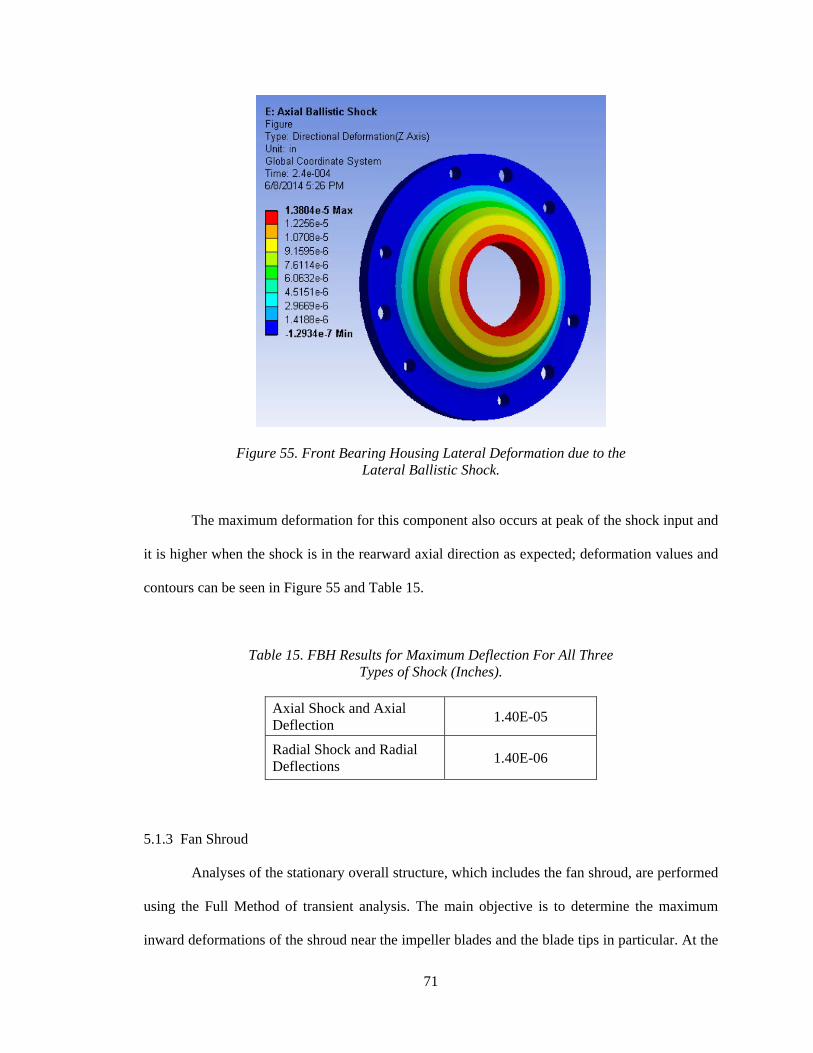
71

Figure 55. Front Bearing Housing Lateral Deformation due to the Lateral Ballistic Shock.

The maximum deformation for this component also occurs at peak of the shock input and

it is higher when the shock is in the rearward axial direction as expected; deformation values and

contours can be seen in Figure 55 and Table 15.

Table 15. FBH Results for Maximum Deflection For All Three Types of Shock (Inches).

Axial Shock and Axial Deflection 1.40E-05

Radial Shock and Radial Deflections 1.40E-06

5.1.3 Fan Shroud

Analyses of the stationary overall structure, which includes the fan shroud, are performed

using the Full Method of transient analysis. The main objective is to determine the maximum

inward deformations of the shroud near the impeller blades and the blade tips in particular. At the

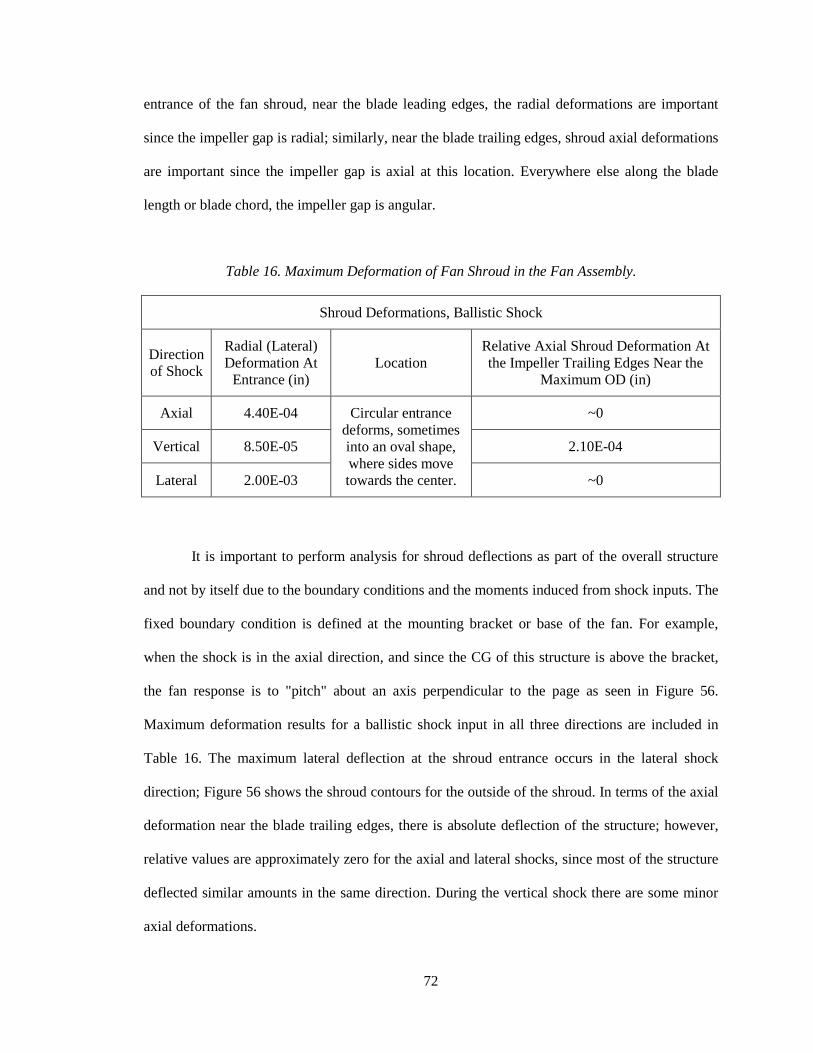
72

entrance of the fan shroud, near the blade leading edges, the radial deformations are important

since the impeller gap is radial; similarly, near the blade trailing edges, shroud axial deformations

are important since the impeller gap is axial at this location. Everywhere else along the blade

length or blade chord, the impeller gap is angular.

Table 16. Maximum Deformation of Fan Shroud in the Fan Assembly.

Shroud Deformations, Ballistic Shock

Direction of Shock

Radial (Lateral) Deformation At

Entrance (in) Location

Relative Axial Shroud Deformation At the Impeller Trailing Edges Near the

Maximum OD (in)

Axial 4.40E-04 Circular entrance deforms, sometimes into an oval shape, where sides move towards the center.

~0

Vertical 8.50E-05 2.10E-04

Lateral 2.00E-03 ~0

It is important to perform analysis for shroud deflections as part of the overall structure

and not by itself due to the boundary conditions and the moments induced from shock inputs. The

fixed boundary condition is defined at the mounting bracket or base of the fan. For example,

when the shock is in the axial direction, and since the CG of this structure is above the bracket,

the fan response is to "pitch" about an axis perpendicular to the page as seen in Figure 56.

Maximum deformation results for a ballistic shock input in all three directions are included in

Table 16. The maximum lateral deflection at the shroud entrance occurs in the lateral shock

direction; Figure 56 shows the shroud contours for the outside of the shroud. In terms of the axial

deformation near the blade trailing edges, there is absolute deflection of the structure; however,

relative values are approximately zero for the axial and lateral shocks, since most of the structure

deflected similar amounts in the same direction. During the vertical shock there are some minor

axial deformations.

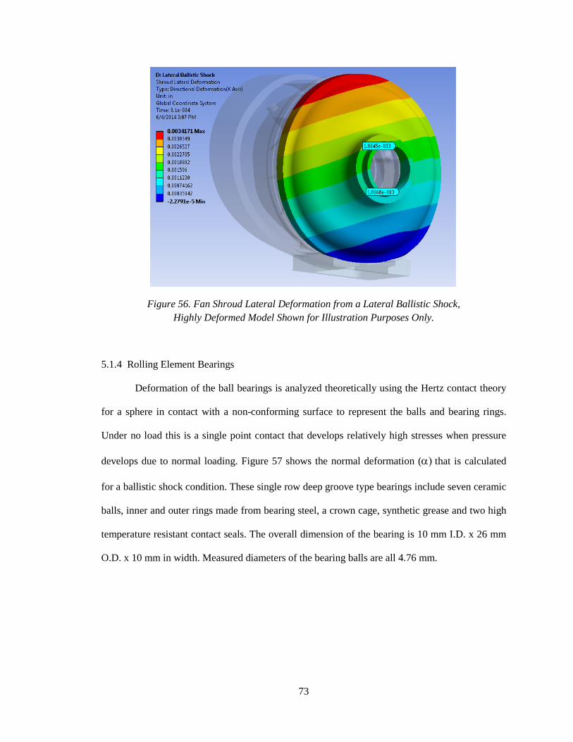
73

Figure 56. Fan Shroud Lateral Deformation from a Lateral Ballistic Shock, Highly Deformed Model Shown for Illustration Purposes Only.

5.1.4 Rolling Element Bearings

Deformation of the ball bearings is analyzed theoretically using the Hertz contact theory

for a sphere in contact with a non-conforming surface to represent the balls and bearing rings.

Under no load this is a single point contact that develops relatively high stresses when pressure

develops due to normal loading. Figure 57 shows the normal deformation (α) that is calculated

for a ballistic shock condition. These single row deep groove type bearings include seven ceramic

balls, inner and outer rings made from bearing steel, a crown cage, synthetic grease and two high

temperature resistant contact seals. The overall dimension of the bearing is 10 mm I.D. x 26 mm

O.D. x 10 mm in width. Measured diameters of the bearing balls are all 4.76 mm.

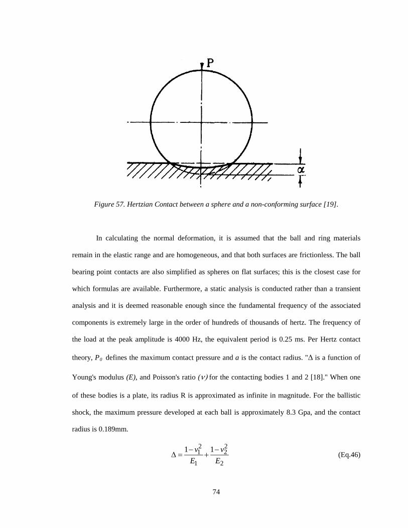
74

Figure 57. Hertzian Contact between a sphere and a non-conforming surface [19].

In calculating the normal deformation, it is assumed that the ball and ring materials

remain in the elastic range and are homogeneous, and that both surfaces are frictionless. The ball

bearing point contacts are also simplified as spheres on flat surfaces; this is the closest case for

which formulas are available. Furthermore, a static analysis is conducted rather than a transient

analysis and it is deemed reasonable enough since the fundamental frequency of the associated

components is extremely large in the order of hundreds of thousands of hertz. The frequency of

the load at the peak amplitude is 4000 Hz, the equivalent period is 0.25 ms. Per Hertz contact

theory, P0 defines the maximum contact pressure and a is the contact radius. "∆ is a function of

Young's modulus (E), and Poisson's ratio (ν) for the contacting bodies 1 and 2 [18]." When one

of these bodies is a plate, its radius R is approximated as infinite in magnitude. For the ballistic

shock, the maximum pressure developed at each ball is approximately 8.3 Gpa, and the contact

radius is 0.189mm.

2 21 2

1 2

1 1v vE E− −

∆ = + (Eq.46)

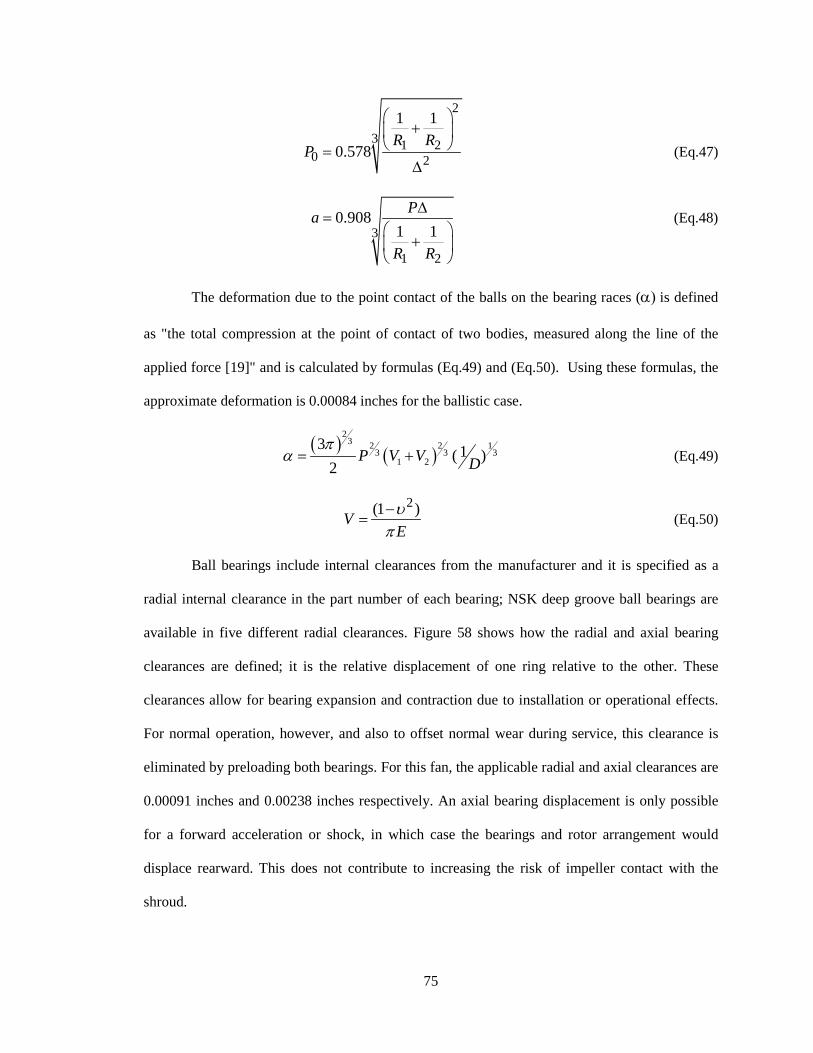
75

2

3 1 20 2

1 1

0.578R

PR

+

=∆

(Eq.47)

3

1 2

0.9081 1

Pa

R R

∆=

+

(Eq.48)

The deformation due to the point contact of the balls on the bearing races (α) is defined

as "the total compression at the point of contact of two bodies, measured along the line of the

applied force [19]" and is calculated by formulas (Eq.49) and (Eq.50). Using these formulas, the

approximate deformation is 0.00084 inches for the ballistic case.

( ) ( )

23 2 2 1

3 3 31 2 (

3 1 )2

V V DPπ

α += (Eq.49)

2(1 )V

Eυ

π−

= (Eq.50)

Ball bearings include internal clearances from the manufacturer and it is specified as a

radial internal clearance in the part number of each bearing; NSK deep groove ball bearings are

available in five different radial clearances. Figure 58 shows how the radial and axial bearing

clearances are defined; it is the relative displacement of one ring relative to the other. These

clearances allow for bearing expansion and contraction due to installation or operational effects.

For normal operation, however, and also to offset normal wear during service, this clearance is

eliminated by preloading both bearings. For this fan, the applicable radial and axial clearances are

0.00091 inches and 0.00238 inches respectively. An axial bearing displacement is only possible

for a forward acceleration or shock, in which case the bearings and rotor arrangement would

displace rearward. This does not contribute to increasing the risk of impeller contact with the

shroud.

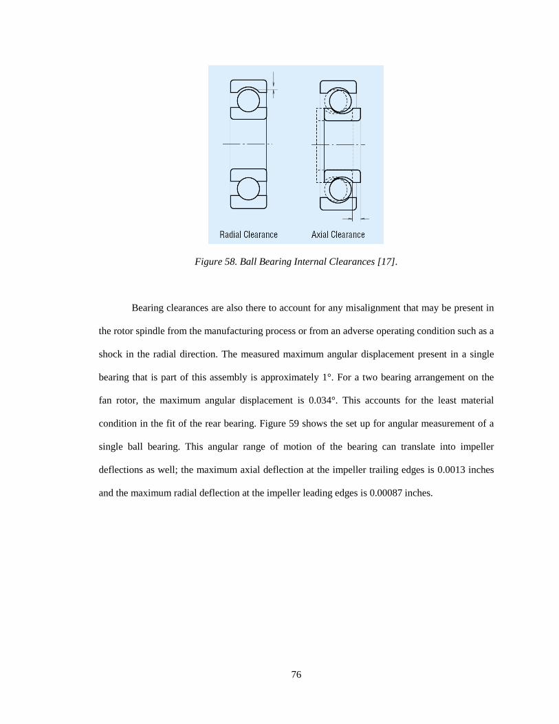
76

Figure 58. Ball Bearing Internal Clearances [17].

Bearing clearances are also there to account for any misalignment that may be present in

the rotor spindle from the manufacturing process or from an adverse operating condition such as a

shock in the radial direction. The measured maximum angular displacement present in a single

bearing that is part of this assembly is approximately 1°. For a two bearing arrangement on the

fan rotor, the maximum angular displacement is 0.034°. This accounts for the least material

condition in the fit of the rear bearing. Figure 59 shows the set up for angular measurement of a

single ball bearing. This angular range of motion of the bearing can translate into impeller

deflections as well; the maximum axial deflection at the impeller trailing edges is 0.0013 inches

and the maximum radial deflection at the impeller leading edges is 0.00087 inches.

77

Figure 59. Maximum Angular Displacement Measurement in a Single 10x26x8 mm Ball Bearing.

A steady state thermal analysis is also conducted on the impeller to determine the thermal

growth due to increased temperatures during operation. Heat rejection through the impeller is a

relatively small percentage compared to the total motor energy losses; regardless, it is important

to determine how much these thermal effects contribute to closure of the blade tip clearances. A

forced air convection of 100 W/(m2K) is assumed on the front face of the impeller as well as 15

W energy dissipation. Radial growth at the tip of the blades leading edges at the entrance of the

fan shroud is 0.0004 inches. Axial growth at the tip of the blades trailing edges is approximately

0.0001 inch since it is at a larger distance from the heat source.

5.1.5 Final Analytical Results for the Mixed Flow Fan

Taking all previous analytical results for the mixed flow fan into account, and as shown

in Tables 17 and 18, the maximum radial and axial blade tip clearance closure during a ballistic

78

shock is 0.0042 inches and 0.0034 inches respectively. The radial closure occurs at the entrance

of the fan shroud at the leading edges; the axial closure occurs near the tip of the blades trailing

edges.

Table 17. Addition of All Radial Shock Deformation Results That Affect Tip Clearance.

Total Maximum Radial Closure of Blade Tip Clearance At Leading Edges At the Shroud Entrance. (Radial = Lateral or Vertical)

From A Vertical Ballistic Shock (in) = 4.15E-03

From An Axial Ballistic Shock (in) = 1.71E-03

Table 18. Addition of All Axial Shock Deformation Results That Affect Tip Clearance.

Total Maximum Axial Closure of Blade Tip Clearance At Trailing Edges

From A Vertical Ballistic Shock (in) = 2.79E-03

From An Axial Ballistic Shock (in) = 3.39E-03

5.2 Experimental Results for the H200 Mixed Flow Fan

The H200 fan was subjected to shock tests per MIL STD 810 and as described by Table

13. This machine was instrumented with three tri-axial accelerometers. One was located on the

outside of the impeller shroud, one on the outside of the diffuser and one on the tail cone, shown

in Figure 60. One uni-axial accelerometer was mounted to the slip table as the base input for the

signal control. A tachometer was used to measure the fan speed. The H200 fan was run at a

speed of 18,750 RPM during the shock tests and remained operational after the tests. After all the

tests were completed, a detailed tear-down inspection of the unit was performed. The bearing

assemblies were returned to the bearing manufacturer for detailed inspection.

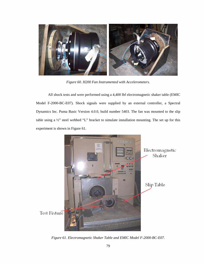
79

Figure 60. H200 Fan Instrumented with Accelerometers.

All shock tests and were performed using a 4,400 lbf electromagnetic shaker table (EMIC

Model F-2000-BC-E07). Shock signals were supplied by an external controller, a Spectral

Dynamics Inc. Puma Basic Version 4.0.0, build number 5403. The fan was mounted to the slip

table using a ½” steel webbed “L” bracket to simulate installation mounting. The set up for this

experiment is shown in Figure 61.

Figure 61. Electromagnetic Shaker Table and EMIC Model F-2000-BC-E07.

80

A total of twenty-seven shocks were imparted: three different types of shocks, three times

each in succession, in three separate orthogonal directions. The directions of the shocks were

axial, vertical, and lateral. Fan responses to the three shock inputs are shown in Figures 62

through 64; they show the response to a lateral ballistic shock, lateral gun firing shock, and lateral

road load shock. Shock 1, 2, and 3 represent the three consecutive shocks. Figure 62 shows a

filtered ballistic signal and the amplitude of the ballistic shock going slightly above 50 g but

remains within the specified limits. Figures 63 and 64 show unfiltered signals for the gun firing

and road load shock, respectively. As can be seen in these responses, there is a better control on

the amplitude versus the pulse width of the shock. After shock testing, the fan was tested and

showed no adverse effects in motor or aerodynamic performance.

Figure 62. Fan Response to Ballistic Shock in the Lateral Direction.

81

Figure 63. Fan Response to Gun Firing Shock in the Lateral Direction.

Figure 64. Fan Response to Road Load Shock in the Lateral Direction.

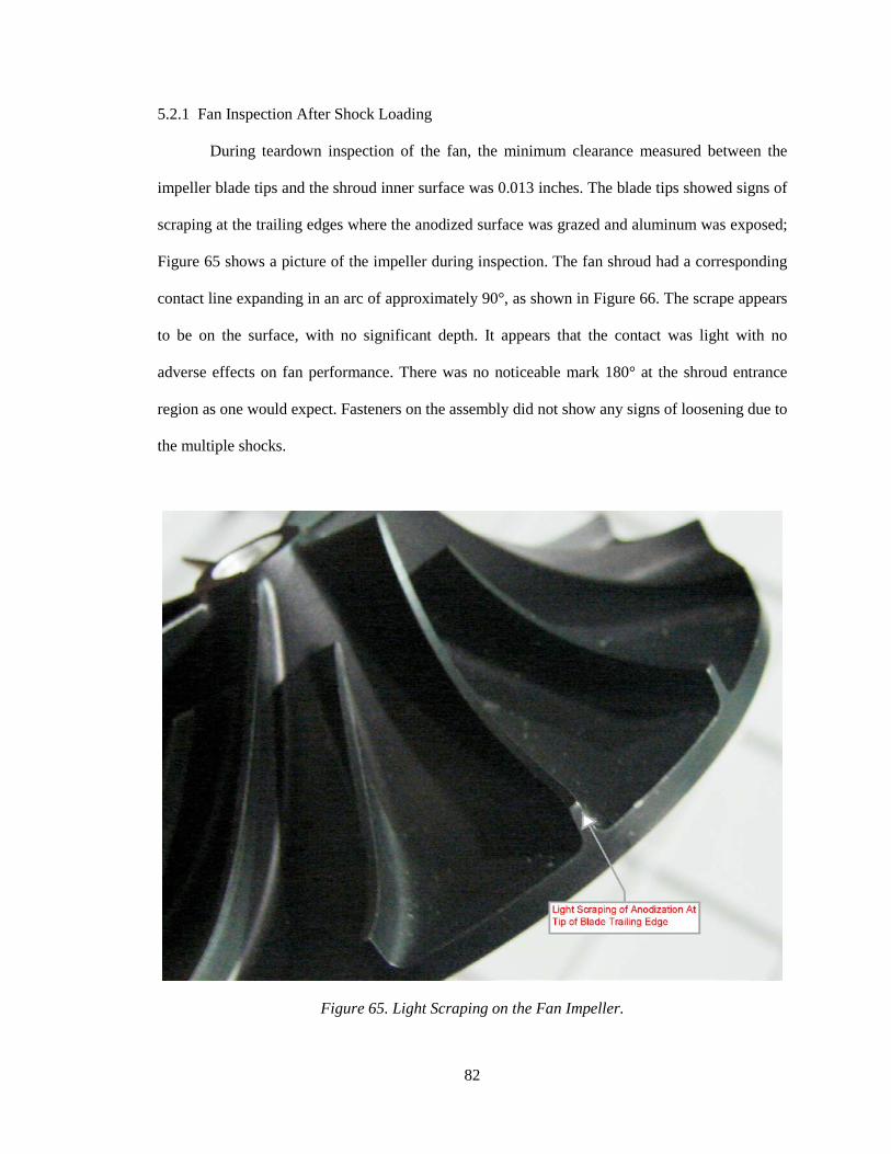
82

5.2.1 Fan Inspection After Shock Loading

During teardown inspection of the fan, the minimum clearance measured between the

impeller blade tips and the shroud inner surface was 0.013 inches. The blade tips showed signs of

scraping at the trailing edges where the anodized surface was grazed and aluminum was exposed;

Figure 65 shows a picture of the impeller during inspection. The fan shroud had a corresponding

contact line expanding in an arc of approximately 90°, as shown in Figure 66. The scrape appears

to be on the surface, with no significant depth. It appears that the contact was light with no

adverse effects on fan performance. There was no noticeable mark 180° at the shroud entrance

region as one would expect. Fasteners on the assembly did not show any signs of loosening due to

the multiple shocks.

Figure 65. Light Scraping on the Fan Impeller.

83

Figure 66. Light Scrape Mark on Fan Shroud.

The complete rotor assembly was also sent to the bearing manufacturer for inspection.

The front and rear bearings were removed and disassembled for full inspection. Both bearings

showed false brinelling with no discernible depth present, as well as a typical amount of out of

roundness on the ball traces. Both the balls and the retainers remained in good condition. Figure

67 shows a photo from the inspection process where axial brinells can be spotted.

84

Figure 67. Inspection of Bearing Rings Showing Axial Brinells.

5.3 Summary of Chapter 5

The total calculated radial and axial closure of tip clearance is 0.0042 and 0.0034 inches

respectively. These are values for the ballistic shock for which the fan components showed the

largest deformation from the shock response. The radial closure was calculated at the entrance of

the fan shroud near the blade's leading edges and the axial closure was calculated at the blades

trailing edges. The measured minimum radial clearance calculated before experimental shock

testing was 0.013 inches. There is indication of blade contact against the shroud; however, shock

analyses and impeller thermal analysis results account for closure of 32.3% of the measured tip

clearance. From inspection of the bearing rings on the front bearing housing, the axial brinells on

the race shoulder indicate there was significant axial displacement of the bearing balls. This

bearing deformation is believed to account for most of the remaining 67.8% of tip clearance

85

closure and contact with the fan shroud. Thermal effects could also have contributed to increased

deformations, increased clearances, and loosening of shrink fits for parts with dissimilar metals,

such as the motor support and the bearing housings.

86

CHAPTER 6

CONCLUSION

This study of shock loading includes a new graphical representation of shock response to

pulse width variation through the finite element method. It is a great new tool for understanding

the sensitivity of any structure to a particular pulse width of a shock input. Three different case

studies were dissected and they all show the same pattern; when the input has a similar time to

maximum acceleration as the natural period of the structure, the amplitude of the response is

relatively large. Furthermore, using Ansys to solve FEA models offered an opportunity to study

and efficiently solve complex analyses, as is the case with rotational machinery. In these types of

cases, such as the Baseline Impeller case study, we have structures experiencing centrifugal and

impulse loading and responding with a great variety of blade and disk modes. In this case study,

the Full Method and the Mode Superposition Method are explored along with their strengths and

complexities and re-introduced as tools for current and future practicing engineers.

Providing the background for this report, Chapter 3 includes a great correlation between

analytical and experimental results, where the Euler-Bernoulli theory and finite element analysis

are used to solve modal and shock loading of cantilevered beams. This knowledge is used in

Chapter 4 of this report where blades of the baseline impeller are modeled as cantilevered beams

for extracting the mode shapes and natural frequencies, a process that is currently being used in

the preliminary design of bladed impellers. In the last chapter, FEA and classical theory are used

to analyze a mixed flow fan undergoing shock loading; both the Full Method and the Mode

Superposition Method were utilized to help in understanding how real systems respond to these

types of inputs.

87

REFERENCES

[1] Lee, Huei-Huang. Finite Element Simulations with ANSYS Workbench 14. Mission: SDC Publications, 2012. Print.

[2] Szuladzinski, Gregory. Formulas for Mechanical and Structural Shock and Impact. Boca Raton: Taylor and Francis Group, LLC, 2010. Print.

[3] Inman, Daniel J. Engineering Vibrations. 2nd ed. Upper Saddle River: Prentice-Hall, Inc., 2001. Print.

[4] Repetto, C. E., Roatta, A., Welti, R. J. "Forced Vibrations of a Cantilever Beam." European Journal of Physics 33 (2012): 1187-1195. Print.

[5] Haukaas, Terje. "Euler-Bernoulli Beams." University of British Columbia, Nov. 2012. Web. 02 Mar. 2014.

[6] Siscribd. “Transverse Vibration of a Cantilever Beam.” Scribd 08 Aug. 2012. Web. 02 Mar. 2014.

[7] Whitney, Scott. “Vibrations of Cantilever Beams: Deflection, Frequency, and Research Uses.” University of Nebraska-Lincoln, 23 Apr. 1999. Web. 13 Dec. 2013.

[8] Sadd, M. H. Wave Motion and Vibration in Continuous Media. Kingston: University of Rhode Island, 2009. Print.

[9] Majkut, Leszek. “Free and Forced Vibrations of Timoshenko Beams Described by Single Difference Equations.” Journal of Theoretical and Applied Mechanics 47.1 (2009): 193-210. Print.

[10] Tongue, Benson H. Principles of Vibration. New York: Oxford University Press, Inc, 1996. Print.

[11] Park, K. C. "Appendix C. Analytical Natural Vibration Modes and Mode Shapes of a Cantilever Beam." University of Colorado, 12 Feb. 2002. Web. 05 Mar. 2014.

[12] Yang, Bingen. Stress, Strain, and Structural Dynamics: An Interactive Handbook of Formulas, Solutions, and Matlab Toolboxes. San Diego: Elsevier Inc., 2005. Print.

[13] Soedel, Werner. Sound and Vibration of Positive Displacement Compressors. Boca Raton: CRC Press, 2006. Print.

[14] ANSYS, Inc. Ansys Mechanical APDL Structural Analysis Guide. Release 14.5. Canonsburg: SAS IP, Inc., 2012. Print.

[15] J. Luo, D. W. Shu, B. J. Shi, and B. Gu. “The Pulse Width Effect on the Shock Response of the Hard Drive Disk.” International Journal of Impact Engineering 34 (2007): 1342-1349. Print.

88

[16] Rubin, Sheldon. Shock and Vibration Handbook. 2nd ed. Ed. Cyril M. Harris and Allan G. Piersol. New York: McGraw-Hill, 2002. Print.

[17] Rolling Bearing Catalog. CAT.No. E1102j ed. Japan: NSK Ltd., 2005. Print.

[18] Juvinal, Robert C. and Marshek, Kurt M. Fundamentals of Machine Component Design. 3rd ed. Hoboken: John Wiley & Sons, Inc., 2000. Print.

[19] Puttock, M. J. and Thwaite, E. G. “Elastic Compression of Spheres and Cylinders at Point and Line Contact.”. Commonwealth Scientific and Industrial Research Organization, Austrailia National Standards Laboratory Technical Papter No. 25 (1969): 1-64. Print.

[20] Alexander, J. Edward. “Shock Response Spectrum - A Primer.” Sound and Vibration June (2009): 6-14. Print.

[21] Stapp, J.P. “Effects of Mechanical Force on Living Tissues.” Journal of Aviation Medicine 26.4 (1955): 268-88. Print.

[22] Viano, David C. and King, Albert I. Biomechanics: Principles and Applications. 2nd ed. Ed. Donald R. Peterson and Joseph D. Bronzino. Boca Raton: Taylor & Francis Group, LLC, 2008. Print.

[23] Mohammadi, S. and Hassanirad, A. “Applied and Theoretical Cantilever Beam Free Vibration Analysis.” World Academy of Science, Engineering and Technology 61.305 (2012): 1619-1622. Print.

[24] Haran, Shivan. “Second Order Systems: Vibrating Cantilever Beams.” Arkansas State University: ME 3504 Process Monitoring and Control, 03 Nov. 2005. Web. 02 Mar. 2014.

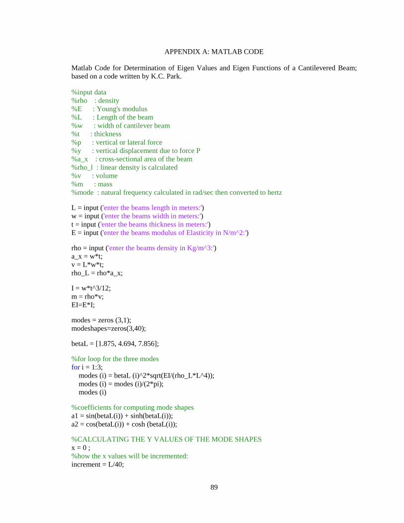
89

APPENDIX A: MATLAB CODE

Matlab Code for Determination of Eigen Values and Eigen Functions of a Cantilevered Beam; based on a code written by K.C. Park. %input data %rho : density %E : Young's modulus %L : Length of the beam %w : width of cantilever beam %t : thickness %p : vertical or lateral force %y : vertical displacement due to force P %a_x : cross-sectional area of the beam %rho_l : linear density is calculated %v : volume %m : mass %mode : natural frequency calculated in rad/sec then converted to hertz L = input ('enter the beams length in meters:') w = input ('enter the beams width in meters:') t = input ('enter the beams thickness in meters:') E = input ('enter the beams modulus of Elasticity in N/m^2:') rho = input ('enter the beams density in Kg/m^3:') a_x = w*t; v = L*w*t; rho_L = rho*a_x; I = w*t^3/12; m = rho*v; EI=E*I; modes = zeros (3,1); modeshapes=zeros(3,40); betaL = [1.875, 4.694, 7.856]; %for loop for the three modes for i = 1:3; modes (i) = betaL (i)^2*sqrt(EI/(rho_L*L^4)); modes (i) = modes (i)/(2*pi); modes (i) %coefficients for computing mode shapes a1 = sin(betaL(i)) + sinh(betaL(i)); a2 = cos(betaL(i)) + cosh (betaL(i)); %CALCULATING THE Y VALUES OF THE MODE SHAPES x = 0 ; %how the x values will be incremented: increment = L/40;

90

%beta is betaL/L and is part of the original formula beta = betaL(i)/L; %this j loop runs 40 times and completes, for every run of the i loop for j=1:40 y = a1*(cosh(x) - cos(x))- a2*(sinh(x) - sin(x)) ; x = x + (beta)*increment; modeshapes(i,j) = y; end; end; %x values denoted by a beam span beamspan = (1:40)*(L/40); %Plot of the First Mode Shape figure (1); ymax = max (abs (modeshapes(1,:))); plot (beamspan, modeshapes(1,:)/ymax); grid on; ylabel ('Modeshape Amplitude'); xlabel ('Beam Span') title ('Mode Shape of the First Mode of a Cantilever Beam'); legend([' First Mode Frequency =', num2str(modes(1))]); %Plot of the Second Mode Shape figure (2); ymax = max (abs (modeshapes(2,:))); plot (beamspan, modeshapes(2,:)/ymax); grid on; ylabel ('Modeshape Amplitude'); xlabel ('Beam Span') title ('Mode Shape of the Second Mode of a Cantilever Beam'); legend([' Second Mode Frequency =', num2str(modes(2))]); %Plot of the Third Mode Shape figure (3); ymax = max (abs (modeshapes(3,:))); plot (beamspan, modeshapes(3,:)/ymax); grid on; ylabel ('Modeshape Amplitude'); xlabel ('Beam Span') title ('Mode Shape of the Third Mode of a Cantilever Beam'); legend([' Third Mode Frequency =', num2str(modes(3))]); %figure 4 below show values for deflection, that are Not Normalized figure (4); plot (beamspan, modeshapes(1,:)); grid on; ylabel ('modeshape amplitude'); xlabel ('beam span') title ('Mode Shape of the First Mode of a cantilever beam Not Normalized'); legend([' first mode frequency =', num2str(modes(1))]);