A STUDY OF SHALE GAS PRODUCTION AND ITS SUPPLY CHAIN

by

Yuwen Yang

Bachelor of Engineering, Beihang University, Beijing, 2013

Submitted to the Graduate Faculty of

Swanson School of Engineering in partial fulfillment

of the requirements for the degree of

Master of Science in Industrial Engineering

University of Pittsburgh

2016

ii

UNIVERSITY OF PITTSBURGH

SWANSON SCHOOL OF ENGINEERING

This thesis was presented

by

Yuwen Yang

It was defended on

June 23, 2016

and approved by

William E. Hefley, Ph.D., Clinical Professor, Naveen Jindal School of Management, The

University of Texas at Dallas

Bopaya Bidanda, Ph.D., Professor, Department of Industrial Engineering

Thesis Advisor: Jayant Rajgopal, Ph.D., Professor, Department of Industrial Engineering

iii

Copyright © by Yuwen Yang

2016

iv

Over the last few years, shale gas has become one of the most important energy sources in the

United States, and advances in related technologies have led to an unprecedented economic

boom in several parts of the country. On the other hand, the shale gas sector and its unique

extraction technologies are still relatively young, and there are a number of concerns from the

public about several aspects of the shale gas industry such as hydraulic fracturing, methane

emission and waste management. The objective of this thesis is to present a comprehensive and

objective study of shale gas and its entire supply chain, including the various material flows

within it, in order to motivate safety, cost-savings and operational efficiency improvement.

The study begins with an introduction to the basic background of the petroleum, natural

gas and shale gas industry and goes on to describe the process of shale gas production and map

its supply chain, starting with initial exploration to identify a potential drilling location and

ending with the delivery of the natural gas to end-use customers. We present detailed flow of

various materials and when possible, costs in the shale gas supply chain as a first step toward

planning for its efficient operation. We also span a wide range of topics including environmental

effects and safety, public health implications of unconventional gas extraction, the upgraded

equipment and techniques to reduce environmental pollution, the use pattern of shale gas,

fluctuations in its price, and its implications on sustainable energy. We end with a detailed case

A STUDY OF SHALE GAS PRODUCTION AND ITS SUPPLY CHAIN

Yuwen Yang, M.S.

University of Pittsburgh, 2016

v

study of distributed power generation from Marcellus shale, and discuss how natural gas can

play a key role in bridging the gap between coal/petroleum based energy and renewable energy.

As a more reliable and cheaper alternative to renewable energy today, and as a more

environmentally friendly alternative to other fossil fuels such as coal and petroleum, shale gas

has the potential to be a solution to the energy gap in the near future.

vi

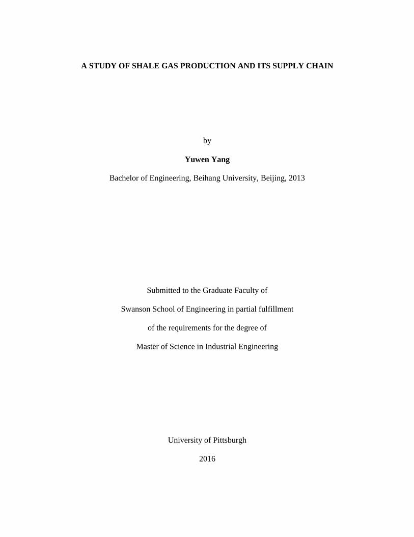
TABLE OF CONTENTS

PREFACE .................................................................................................................................. XII

1.0 INTRODUCTION ........................................................................................................ 1

1.1 PETROLEUM AND NATURAL GAS .............................................................. 1

1.2 SHALE GAS......................................................................................................... 5

1.3 HYDRAULIC FRACTURING ........................................................................... 8

1.4 THE SHALE GAS INDUSTRY ....................................................................... 11

2.0 SHALE GAS SUPPLY CHAIN ................................................................................ 15

2.1 THE TRANSIENT SUPPLY CHAIN .............................................................. 18

2.1.1 Leasing, Acquisition, and Permitting ........................................................ 19

2.1.2 Site Construction ......................................................................................... 19

2.1.3 Drilling ......................................................................................................... 21

2.1.4 Hydraulic Fracturing.................................................................................. 25

2.1.5 Completion................................................................................................... 29

2.2 THE STABLESUPPLY CHAIN ...................................................................... 30

2.2.1 Production ................................................................................................... 31

2.2.2 Processing .................................................................................................... 34

2.2.3 Gas Distribution .......................................................................................... 36

2.2.4 Storage ......................................................................................................... 43

3.0 FLOWS IN THE SUPPLY CHAIN ......................................................................... 46

vii

3.1 MATERIAL FLOWS ........................................................................................ 48

3.1.1 Site Construction ......................................................................................... 48

3.1.2 Drilling ......................................................................................................... 50

3.1.3 Hydraulic Fracturing.................................................................................. 52

3.1.4 Completion................................................................................................... 57

3.2 FINANCIAL FLOWS ....................................................................................... 59

4.0 DISCUSSION AND SUMMARY ............................................................................. 61

4.1 METHANE EMISSION .................................................................................... 61

4.2 USAGE AND PRICE FLUCTUATIONS OF NATURAL GAS ................... 64

4.3 BRIDGING THE GAP ...................................................................................... 73

4.3.1 Background ................................................................................................. 77

4.3.2 The Supply Chains with Distributed Power Generation......................... 79

4.3.3 Economics of Distributed Power Generation ........................................... 81

4.3.4 A Case Study ............................................................................................... 92

4.3.5 Discussion................................................................................................... 105

4.3.6 Limitations ................................................................................................. 107

4.3.7 Conclusion ................................................................................................. 109

4.4 SUMMARY AND CONCLUSIONS .............................................................. 110

4.5 CONTRIBUTIONS AND FUTURE WORK ................................................ 111

APPENDEX A. CHEMICALS IN HYDRAULIC FRACTURING FLUIDS ..................... 114

BIBLIOGRAPHY ..................................................................................................................... 119

viii

LIST OF TABLES

Table 1. Typical Composition of Natural Gas ................................................................................ 3

Table 2. Material Flows in Site Construction ............................................................................... 49

Table 3. By-product in Site Construction ..................................................................................... 50

Table 4. Material Flows in Drilling .............................................................................................. 50

Table 5. By-product in Site Construction ..................................................................................... 52

Table 6. Materials used in Slick Water ......................................................................................... 55

Table 7. Material Flows in Hydraulic Fracturing ......................................................................... 56

Table 8. Material Flows in Completion ........................................................................................ 57

Table 9. By-product in Completion .............................................................................................. 59

Table 10. Estimated Total Cost of a Marcellus Shale Well .......................................................... 60

Table 11. Natural Gas Consumptions by End Use in 2009 and 2015........................................... 67

Table 12. Average Fossil Fuel Power Plant Emission Rates ........................................................ 76

Table 13. List of Notations ........................................................................................................... 84

Table 14. The Gas Supplier/DPP Interface Efficiency ................................................................. 96

Table 15. Electricity Demand Estimates at DLC .......................................................................... 98

Table 16. Each Component of Estimated and Actual Billing ..................................................... 101

Table 17. The DPP/DLC Section Saving .................................................................................... 103

ix

Table 18. Estimated Levelized Cost of Electricity for New Generation Resources ................... 105

Table 19. Comparison of Total Amount of CO2Emissions (tons) .............................................. 106

Table 20. Comparison of Total Cost (US dollar) ........................................................................ 106

Table 21. A Summary of the Various Chemicals Used to Make Hydraulic Fracturing Fluids .. 114

x

LIST OF FIGURES

Figure 1. Range of Conventional and Unconventional Hydrocarbons .......................................... 6

Figure 2. Lower 48 States Shale Plays........................................................................................... 7

Figure 3. U.S. Dry Shale Gas Production ....................................................................................... 8

Figure 4. Hydraulic Fracturing ....................................................................................................... 9

Figure 5.Natural Gas Gross Withdrawals Shares from Shale Gas Wells and Gas Wells ............. 12

Figure 6. Monthly Natural Gas Price in 2015 and 2014 ............................................................... 13

Figure 7. Shale Gas Supply Chain ................................................................................................ 16

Figure 8. Stable Shale Gas Supply Chain ..................................................................................... 17

Figure 9. A Multi-Well Pad with 8 Wells ..................................................................................... 23

Figure 10.Casing and Cement ....................................................................................................... 24

Figure 11. Vertical Well and Directional Well ............................................................................. 26

Figure 12. Natural Gas Production and Delivery.......................................................................... 30

Figure 13. Discrete-time well productivity profile. ...................................................................... 31

Figure 14. Natural Gas Processing Plants and Production Basins, 2009 ...................................... 36

Figure 15. Natural Gas Compressors ............................................................................................ 38

Figure 16. Natural Gas Market Centers and Hubs ....................................................................... 42

Figure 17. Monthly Average Natural Gas Spot Price at Key Trading Hubs ............................... 42

xi

Figure 18.Natural Gas Underground Storage Facilities ................................................................ 44

Figure 19. Natural Gas Storage Levels and Corresponding Prices .............................................. 45

Figure 20. U.S. Methane Emissions by Source, 1990 – 2014 ...................................................... 62

Figure 21. U.S. Methane Emissions, 1990-2014 .......................................................................... 63

Figure 22. Natural Gas Annual Consumption from 2000 to 2015 ................................................ 66

Figure 23. Share of Natural Gas Consumptions by End Use in 2015........................................... 68

Figure 24. Working Gas in Underground Storage ........................................................................ 70

Figure 25. Weekly Lower 48 States Natural Gas in Underground Storage .................................. 70

Figure 26. U.S. Primary Energy Consumption and Projection ..................................................... 76

Figure 27. Midstream Gas Sector ................................................................................................. 79

Figure 28. Natural Gas Cost Components .................................................................................... 81

Figure 29. Distributed Power Generation Model .......................................................................... 83

xii

PREFACE

To my parents

This thesis started with some initial work on the merits of utilizing shale gas locally by using it to

generate electricity and supply customers in the vicinity of the well. Pittsburgh is located in the

heart of the Marcellus shale formation and there is an extremely active shale gas industrial

community in this region; since the demise of steel, shale gas is the first industrial sector that has

seen a significant economic boom in the Western Pennsylvania region. Subsequently, the scope

of the work was therefore extended to studying shale gas production in more detail and to

mapping its entire supply chain. In the process of writing this thesis I have learned a lot and our

initial conceptions of an integrated shale gas industry have certainly changed. We have had

several rig and facility visits, and have interviewed and met with numerous individuals in the

local shale gas sector. These activities have offered us lots of invaluable information.

I would like to thank my committee, Dr. Jayant Rajgopal, Dr. William E. Hefley, and Dr.

Bopaya Bidanda, for their excellent guidance and support during this process, especially my

advisor, Dr. Rajgopal, who gave me myriad help and advice (even on writing).Without him I

would still be suffering in writing the first chapter of the thesis. He was the instructor of my first

Operations Research course, and without him I would not be fond of industrial engineering, be

xiii

on board to conduct research and have the courage and enthusiasm to challenge myself to join

the doctoral program. It is really my pleasure to be his student for another few years.

I would like to acknowledge the Center for Industry Studies at the University of

Pittsburgh for providing me financial support through a grant to Drs. Rajgopal and Hefley. I

also wish to thank Seneca Resources, and specifically, Julianne Heins for offering me invaluable

advice and information; Ms. Heins also facilitated all of our site visits. I thank Rob Boulware,

Alyson Joyce and Bryan Cooley for the wonderful rig visit during heavy snow, along with

Marcus Heller, Barry Guenther, Justin Harsany, Dave Suski and Justin Shultz for the information

and feedback that they provided. Without their cooperation I would not have been able to

complete this study.

I would like to thank Christopher Wissel-Tysonfrom IMG Midstream for supporting us

with technical data and market information and Kenneth Frederick for introducing us to this

relatively new field. I thank the Marcellus Shale Coalition for making information available to

the study team. I also thank my friends, Mamoru Iketani and John Fitzgerald, who were my

colleagues during the summer project.

Finally, I thank my friends for encouraging me and everyone who helped me during the

process.

1

1.0 INTRODUCTION

The goal of this thesis is to describe the process of shale gas production and to study its supply

chain, starting with the exploration of a potential drilling location and ending with the delivery of

the natural gas to end-use customers. The thesis overviews the process and details the flow of

various materials in the shale gas supply chain as a step toward planning for its efficient

operation. It also discusses how natural gas plays a key role in bridging the gap between

coal/petroleum based energy and renewable energy.

1.1 PETROLEUM AND NATURAL GAS

Petroleum is a yellow to black liquid that develops naturally over millennia in geological

formations beneath the surface of the earth. It is extracted and typically, then refined into various

types of fuels. The term “petroleum” often covers naturally occurring unprocessed crude oil as

well as products obtained from it. Crude oil is a mixture of hydrocarbons generated over

centuries from dead plants and animals that lived millions of years ago. It is a fossil fuel that

exists in liquid form in underground pools or reservoirs, within sedimentary rocks, or near the

surface in tar (or oil) sands. Although petroleum products can be obtained from coal or biomass

as well, they are primarily classified as fuels and other products that are made from crude oil as

well as natural gas (EIA, Oil and Petroleum Products, 2015). After crude oil is collected from the

2

ground, it is transported to a refinery where it is processed and separated into different kinds of

useable petroleum products such as gasoline, diesel fuel, heating oil, jet fuel, petrochemical

feedstock, waxes, lubricating oils, and asphalt.

Petroleum products have been used since ancient times. According to Herodotus and

Diodorus Siculus, asphalt was used in the construction of the towers and walls of Babylon more

than 4000 years ago. In addition, oil pits were found near Ardericca (near Babylon), and a pitch

spring was discovered on Zacynthus. There are many allusions to the use of natural gas as

alighting and heating resource in ancient China and Japan. The first mention of petroleum in

America was by Sir Walter Raleigh in 1595, while the first important commercial exploitation of

oil was at Alfreton, Derbyshire by James Young in 1850, when he patented his process for the

manufacture of paraffin. Starting from around the middle of the nineteenth century, the

petroleum industry in the United States began to grow rapidly. The reported crude petroleum

production in the United States was “2000 barrels in 1859; 4,215,000 barrels in 1869; 19,914,146

barrels in 1879; 35,163,513 barrels in 1889; 57,084,428 barrels in 1899; and 126,493,936 barrels

in 1906” (Chisholm, 1910). In 2015, around 3.44 billion barrels of crude oil were produced in the

United States (EIA, Crude Oil Production, 2016).

Natural gas is currently one of the major sources for petroleum-based fuels. It was

naturally formed from the carbon and hydrogen molecules of ancient organic matter millions of

years ago and is currently trapped inside geological formations as a combustible mixture of

various hydrocarbon gases (NaturalGas.org, Overview of Natural Gas, 2013). The appearance of

natural gas started in the Middle East in ancient times when it was viewed as a supernatural

manifestation. It gave the impression of a mysterious fire bursting from fissures in the ground

when it was ignited. Seeping natural gas was found in Iran between 6000 and 2000 BC, and its

3

applications started 2500 years ago in China, where people collected it from natural seeps using

bamboo pipes and used it to boil ocean water to get salt. Natural gas was first known in Europe

when it was discovered in England in 1659. In 1815, natural gas was found in the United States

in Charleston, West Virginia when a salt-brine well was being dug. The first natural gas well was

drilled six years later in 1821, and in 1858, the first natural gas company in the United States was

established in New York. The 19th century was the starting point of the gas industry, and huge

amounts of natural gas were found in Texas and Oklahoma in the early 1900s. After World War

II, the natural gas industry grew rapidly because of the development of natural gas infrastructure.

It also started to replace oil due to the shortages of crude oil in the late 1960s and early 1970s.

Today, natural gas is considered as one of the cleanest, safest, and most efficient sources of

energy (Mokhatab, Poe, & Mak, 2015)

As shown in Table 1, the composition of natural gas in different wells can vary widely

before it is refined, but it typically includes methane, ethane, propane, butane and pentane. As

gas is removed from a reservoir, the compositions might vary even in the same well.

Table 1. Typical Composition of Natural Gas

Methane CH4 70-90%

Ethane C2H6

0-20% Propane C3H8

Butane C4H10

Pentane C5H12

Carbon Dioxide CO2 0-8%

Oxygen O2 0-0.2%

Nitrogen N2 0-5%

Hydrogen sulfide H2S 0-5%

Rare gases A, He, Ne, Xe trace

4

The primary component of natural gas is methane. Methane is a colorless, odorless gas-

form molecule at room temperature (approximately 70°F/21°C) and standard pressure (an

absolute pressure of exactly 100 kPa) made up of one carbon atom and four hydrogen atoms, i.e.,

CH4. Methane is combustible and the reaction between methane and oxygen when methane is

burnt is as follows:

CH4[g] + 2 O2[g] -> CO2[g] + 2 H2O[l] + 891 kJ

Every molecule of methane (CH4) reacts with two molecules of oxygen (O2) in gas form and

produces one molecule of carbon dioxide (CO2) in gas form and a unit of water (H2O) in liquid

form. The reaction also releases a great deal of energy (891 kJ per unit).

Natural gas is referred to as “wet” gas when other hydrocarbons are present along with

methane in significant quantities. After these other hydrocarbons are removed, i.e., when it is

almost pure methane, it is referred to as dry gas. To get to the final customer, gas must be

processed into uniform quality gas that has specific quality measures so that it can be transported

via pipelines, which constitute the main mode of transportation for natural gas.

Characteristics of natural gas are measured in many different ways. As gas, its quantity

can be measured by the volume in cubic feet when it is at standard temperature and pressure.

Production and distribution enterprises usually measure natural gas in thousands of cubic feet

(Mcf), millions of cubic feet (MMcf), or trillions of cubic feet (Tcf). As a supply of energy,

natural gas can also be measured by potential energy output. It is commonly expressed in British

thermal units (Btu): one Btu is the energy required to increase the temperature of one pound of

water at or around 39.2 degrees Fahrenheit by one degree Fahrenheit at normal pressure. When

used to measure gas it corresponds to the amount of natural gas that will produce this exact

amount of energy. Typically, one cubic foot of natural gas corresponds to 1,027 Btus. Finally, for

5

billing purposes natural gas is measured by gas utilities in ‘therms’ when delivered to a

residence. A therm is equivalent to 100,000 Btu, or approximately 97 cubic feet. In addition to

residential use, the natural gas is also commonly used for electric power generation, and as

industrial, commercial, and vehicle fuel.

We present a detailed description of natural gas production in Section 2.2.1, and describe

the processing of natural gas from wellhead gas to dry gas in Section 2.2.2.We then discuss the

distribution and storage of natural gas in Sections 2.2.3 and 2.2.4, respectively. Additionally, in

Chapter 4 we discuss the use and price fluctuation of natural gas and how natural gas can bridge

the gap between coal/petroleum based energy and renewable energy.

1.2 SHALE GAS

As shown in Figure 1, oil and natural gas can be classified as either conventional or

unconventional. This depends upon the geological formations from which it is extracted.

Conventional natural gas can be found in carbonates, sandstones, and siltstones and is typically

located in deep reservoirs and is associated with crude oil. It is generally easier to produce by

releasing gas from several small porous zones in naturally developed rock formations.

Unconventional gas on the other hand, comes from coal (also known as coal-bed methane), tight

gas sands, gas hydrates and shale. The different types of unconventional gas all contain large

amounts of natural gas. However, when compared to conventional reservoir rocks, it is usually

more difficult to extract. In particular, shale gas is the kind of unconventional natural gas

produced from shale, a “fine-grained sedimentary rock that forms from the compaction of silt

6

and clay-size mineral particles” (EIA, Energy in Brief, 2015). Black shale often contains organic

material, and the pores in it can trap the oil and natural gas developed from the organic material.

Figure 1. Range of Conventional and Unconventional Hydrocarbons

Around the year 2000, natural gas started to be produced on a large scale from shale in

the Barnett Shale in north-central Texas. This was pioneered by the Mitchell Energy and

Development Corporation (EIA, Energy in Brief, 2015). During the 1980s and 1990s, Mitchell

Energy experimented with alternative methods of hydraulic fracturing in the Barnett Shale, and

by2000, the firm had developed a hydraulic fracturing technique that could produce commercial

natural gas from the shale. Following Mitchell, other companies began to drill wells in the

Barnett Shale, as a result of which it was producing almost half a trillion cubic feet (Tcf) of

natural gas per year in 2005. As companies developed their confidence in profitable natural gas

production in the Barnett Shale, they started to expand to other shale locations such as

Fayetteville in northern Arkansas, Haynesville in eastern Texas and northern Louisiana,

Woodford in Oklahoma, Eagle Ford in southern Texas, and the Marcellus and Utica Shales in

Ohio, Pennsylvania, West Virginia and New York. Figures 2 and 3 illustrate the distribution of

Conventional

Gas Oil

Unconventional

Coal-bed Methane

Gas

Tight Sands

Gas Oil

Methane Hydrate

Gas

Shale

Gas Oil

7

shale gas plays in the lower forty-eight states and the dry gas production from each kind of shale

between 2000 and 2016. Today, advanced technologies are able to provide more accurate

estimates of reservoir capacities and are making production of unconventional natural gas much

easier and more efficient. In particular, hydraulic fracturing is playing the most important role in

shale gas production.

Figure 2. Lower 48 States Shale Plays

(EIA, Energy in Brief, 2015)

8

Figure 3. U.S. Dry Shale Gas Production

(EIA, Energy in Brief, 2015)

1.3 HYDRAULIC FRACTURING

Hydraulic fracturing (also called hydrofracturing, hydrofracking, fracking or frac’ing) is a

reservoir stimulation technique that uses pressurized liquid to fracture the rock. As shown in

Figure 4, the processes involved in hydraulic fracturing include the high-pressure injection of

hydraulic fracturing fluid - primarily water, along with a mixture of sand or ceramic beads to

serve as a propping agent, and chemicals that mainly serve to reduce friction -through a

wellbore, and a horizontal casing that is perforated to allow the fluid to flow through the

perforations and create deep cracks in the rock formations that contains natural gas. After the

hydraulic pressure is removed from the wellhead, natural gas begins to flow up to the well

(Gandossi, 2013).

9

Figure 4. Hydraulic Fracturing

(EPA, The Hydraulic Fracturing Water Cycle, 2016)

Although the term “hydraulic fracturing” started to become more common around 2000,

when this process began to be used to produce commercial natural gas in the Barnett Shale in

north-central Texas, the technique itself is not totally new. Hydraulic fracturing has been a well-

established technique for more than 6 decades. The first use of hydraulic fracturing as a

stimulation technique was in 1949 by Stanolind Oil. Since then, close to 2.5 million fracture

treatments have been used worldwide in approximately 60% of all wells drilled today, increasing

the production rate and adding to the US recoverable reserves of oil by at least 30% and to the

recoverable reserves of gas by 90%.

Fracturing can be traced back to the 1860s when liquid (and subsequently, solidified)

nitroglycerin (NG) was used to stimulate hard and shallow rock wells in Pennsylvania, New

10

York, Kentucky, and West Virginia (Watson, 1910).Although NG was extremely hazardous, it

was spectacularly successful for oil well shooting, where the objective was to separate the oil-

bearing formation to increase both initial flow and subsequent oil recovery. The same fracturing

principle was soon used with similar effectiveness to water and gas wells. In the 1930s, people

started to try to inject fluids (acid) that were not explosive into the ground to stimulate a well and

leave a flow channel to the well, thus enhancing its productivity (Montgomery & Smith, 2010).

In 1947, Floyd Farris of Stanolind Oil and Gas Corporation (Amoco) performed in-depth

research to establish a relationship between observed well performance and treatment pressures.

Based on this study, Farris came up with the idea of hydraulically fracturing a formation (rock,

for example) to promote production from oil and gas wells. In 1948, the hydraulic fracturing

process was broadly recognized by the oil and gas industry, thanks to the paper written by J.B.

Clark of Stanolind Oil. A year later, in 1949, a patent was issued with an exclusive license

granted to the Halliburton Oil Well Cementing Company (HOWCO) to use the new hydraulic

fracturing technique. HOWCO performed the first two commercial fracturing treatments. The

first treatment cost $900 and was in Stephens County, Oklahoma, and the second cost $1,000 and

was performed in Archer County, Texas on March 17, 1949, using lease crude oil and a mixture

of gasoline, crude, and 100 to 150 lbm of sand. Soon after that, 332 wells were treated, and the

average production was increased by 75%. Applications of the fracturing process rose rapidly

and increased the oil supply in the United States. During the middle 1950s, treatments were used

in more than 3,000 wells within a month for stretches. In 2008, more than 50,000 hydraulic

fracturing stages were completed at a cost of between $10,000 and $6 million around the world.

In addition, a single well usually has from 8 to more than 40 different stages (Montgomery &

Smith, 2010).

11

However, although hydraulic fracturing is not totally new, the technique is constantly

evolving and expanding at an unprecedented rate, so that the industry is larger than ever.

Directional drilling and new additional chemicals are being applied and the amount of water used

is much larger (Crawford, 2013).In the past, the average fracture treatment only contained

approximately 750 gal of fluid and 400 lbm of sand, while average fracture treatment today use

nearly 60,000 gal of fluid and 100,000 lbm of propping agent. Some of the largest treatments

even exceed 1 million gal of fluid and 5 million lbm of propping agent. Similarly, hydraulic

horsepower (hhp) per treatment has increased from approximately 75 hhp to more than 1,500

hhp, and in some cases it is even around 15,000 hhp (Montgomery & Smith, 2010).

We provide a detailed description of hydraulic fracturing technologies and treatment in

Section 2.1.4.

1.4 THE SHALE GAS INDUSTRY

Shale gas has become an important natural gas resource in a booming expansion within the

United States due to the application of new techniques such as horizontal drilling and hydra-

fracking. The development of the industry has had a huge impact on the US economy and

society, and its future expansion is expected to be rapid.

As shown in Figure 5, in 2007, when shale gas was first considered as a supply of natural

gas by EIA, only 8.07% of natural gas gross withdrawals were from shale gas wells, but by 2014,

the proportion had rapidly risen to 43.88%. This was matched by a decrease in natural gas gross

withdrawals from traditional gas wells from 60.79% to 33.13% (EIA, Natural Gas Gross

Withdrawals and Production, 2016).

12

Figure 5.Natural Gas Gross Withdrawals Shares from Shale Gas Wells and Gas Wells

Data Source: (EIA, Natural Gas Gross Withdrawals and Production, 2016)

The shale gas industry has resulted insignificant direct and indirect economic effects in

the form of major enhancements to opportunities in job creation, fiscal recovery, infrastructure

optimization, economic sustainability and viability (Seydor, et al., 2012). Due to this fact and its

environmental advantages over coal and to a lesser extent, over petroleum, a long-term increase

in shale gas development is predicted for the future. Capital of nearly $1.9 trillion is expected to

be invested in shale gas, leading the share of shale gas to reach an expected 60% of total natural

gas production, and to the support of nearly 1.6 million jobs by 2035 (IHS Global Insight, 2011).

However, the industry is also now witnessing a different set of forecasts for the future

from some sources because of the trend of declining natural gas prices since 2007, when shale

well drilling started to expand on a major scale. According to the U.S. Energy Information

0.00%

10.00%

20.00%

30.00%

40.00%

50.00%

60.00%

70.00%

2007 2008 2009 2010 2011 2012 2013 2014

Shale Gas Wells

Traditional Gas Wells

13

Administration (EIA, Natural Gas Prices, 2016), the wellhead price, before it discontinued being

estimated in January 2013, had dropped by nearly 60% from $6.25 to $2.66. From 2007 to 2015,

the average residential price in a calendar year had dropped from $13.08 to $10.38; the yearly

commercial price had decreased from $11.34 to $7.89; the yearly industrial price had dropped

from $7.68 to $3.84; and the price of gas used for electric power generation had fallen from

$7.31 to $3.37, respectively. In particular, the monthly average prices in 2015were consistently

trending lower than those in the same month in 2014, as illustrated in Figure 6. From the

viewpoint of profitability, the aforementioned fact is increasing the interest in cost-savings and

operational efficiency improvement, which requires a comprehensive understanding of the shale

gas supply chain from the extraction at the gas well to the distribution of final product to the end

customer.

Figure 6. Monthly Natural Gas Price in 2015 and 2014

Data Source: (EIA, Natural Gas Prices, 2016)

Residential, 2014

Residential, 2015

Commercial, 2014

Commercial, 2015

Industrial, 2014

Industrial, 2015

Electric, 2014

Electric, 2015

2

4

6

8

10

12

14

16

18

Jan Feb Mar Apr May Jun Jul Aug Sep Oct Nov Dec

$ p

er T

ho

usa

nd

Cu

bic

Fee

t

14

Prior research has explored the direct economic impact of the shale gas value chain at the

well. This work was based on extensive field research, including a site visit and interviews with

industry participants in Pennsylvania, which has the majority of Marcellus Shale gas reserves

(Hefley, et al., 2011). In other work the major supply chain components, supplier resources and

characteristics were identified and analyzed from the leasing, acquisition and permitting of a

shale gas well to the natural gas distribution and marketing stages (Seydor, et al., 2012). This

work also mainly focused on Pennsylvania and its neighborhood area. Cafaro & Grossmann use

a case study with actual data to analyze the supply chain strategy related to new facilities

location and capacity, determining the number of shale gas wells to run, and water management

during drilling (Cafaro & Grossmann, 2014). While these studies have focused on various stages

or aspects of the supply chain, there is no comprehensive work on the entire supply chain,

including the various material, information and financial flows within it, a mapping of the value

stream from source to customer, and the linking of the supply chain to the external environment

in order to reach cost-savings and operational efficiency improvement. Addressing some of

these issues is one of the goals of this research.

The basic concepts behind a supply chain –and the shale gas supply chain in particular –

are introduced at the beginning of Chapter 2. We consider the supply chain in two separate

stages – a transient one and a stable one – and a detailed description of each is provided in the

rest of this chapter. Their associated material flows are discussed in Chapter 3. Finally, methane

emission, usage patterns and price fluctuations of natural gas, and how natural gas plays a key

role in bridging the gap between coal/petroleum based energy and renewable energy are

discussed in Chapter 4.

15

2.0 SHALE GAS SUPPLY CHAIN

A supply chain is defined as the network of operations performed by companies or organizations,

which connect the suppliers to the end-use customers; it requires the management of material,

information and financial flows across all the players involved in the network (Nahmias &

Olsen, 2015). Traditionally called logistics, the aforementioned management issues emerged

with the industrial revolution; however, the term supply chain management is relatively recent

and dates to the late 1980s. The goal of supply chain management is to achieve a balance

between low operational costs and a high level of service, since in most cases simultaneously

optimizing both of these is not feasible. Common topics in supply chain management include

sourcing, inventory control, production planning, distribution, and sales.

A supply chain is typically identified as three segments. First, the upstream segment is

where we source and procure raw materials, components, and subcomponents from external

suppliers. Second, the midstream segment is where actual manufacturing and assembly take

place. Finally, the downstream segment is where distribution and sales to the customer take

place.

As shown in Figure 7, the uniqueness of the shale gas supply chain makes it necessary to

further divide it into two separate supply chains according to the status of gas wells, and each of

these two chains is studied in more detail in the following sections.

16

Figure 7. Shale Gas Supply Chain

1) The former, or transient supply chain, describes the segments from the

exploration of a potential drilling location until the completion of well construction and the

beginning of production. Although this supply chain exists only for a limited amount of time for

a given well, it is replicated at multiple locations over time and is significant because this is the

specific aspect in which shale gas with its unique drilling approach is different from

conventionally produced natural gas. Critical environmental issues, pad location planning, and

water and chemicals management during hydraulic fracturing are examples of important issues in

this supply chain.

2) The latter, or stable supply chain, corresponds to the production of gas in steady

state and its sales to the end customers. This is largely similar to the supply chain for

conventional gas wells, but the boom in shale gas production and the large quantities of gas

being injected into the market presents significant opportunities in locations such as the

Marcellus Shale region. Figure 8 depicts the facilities involved in the stable supply chain. The

upstream segment of the stable supply chain corresponds to the production section at the

17

wellhead. The midstream segment involves the processing and storage sections. The downstream

segment corresponds to the distribution to different types of gas consumers. While our focus is

not on this supply chain because it is not specific to shale gas, we do study the downstream

portion a little further because of the effect that the increased production of shale gas is having

on consumption by the end user.

Figure 8. Stable Shale Gas Supply Chain

Upstream

Gas well Processing Plant

Wellhead Gas

Ethane

Propane

Butane

Gasoline

Intra/Interstate Gas Pipeline

Gas Consumers

Compressor Station

Hub & Storage Station

Dry Gas

Midstream Downstream

18

2.1 THE TRANSIENT SUPPLY CHAIN

The transient supply chain refers to the supply chain that exists for the duration from when

exploration commences to when construction and fracking of the well are completed and steady

gas flow commences. It is distinct from other natural gas supply chains because of the unique

characteristics of horizontal drilling and hydraulic fracturing. The typical transient supply chain

for shale gas starts with the exploration phase where potential well locations are evaluated. After

the geological evaluation and the identification of the well site, the next steps are leasing,

acquisition and permitting. Once a permit is issued, site preparation and construction can be

started. After the site has been prepared and the well pad has been completed we come to the two

key parts of the transient supply chain: (horizontal) drilling and hydraulic fracturing. With the

latter, issues such as the volume of water usage, quality of produced water, and disposal and

reuse of water need to be considered carefully. When hydraulic fracturing is done, and the

completion of the site is accomplished, the well is ready to produce gas at a steady rate.

The average time from the exploration of a potential gas well site to its completion

normally ranges from approximately 18 months to 2 years. The initial stages of exploration,

leasing and permitting, and site construction take up a majority of this time. Once the drilling of

the well begins, the time needed to finish drilling is relatively small and this time has continued

to decrease with improvements in technology. It used to take as much as 20 to 30 days on

average to drill one well, so that drilling a multi-well pad with eight wells for example, could

take several months. While there are variations that depend on the geology of the site, the time to

drill a well has been decreasing and today it could be as low as7 days. A pad usually has 6 to 15

wells depending upon the geological features of its location. Fracturing and completion both

takes several weeks.

19

2.1.1 Leasing, Acquisition, and Permitting

The first stage in the transient chain corresponds to the identification of a potential site at which

to drill a gas well, when geologists determine which locations might contain a gas reservoir.

Once a location is identified, the shale gas well operator must obtain top land access and mineral

rights. A fixed percentage of revenues from produced gas are paid to the land-owner as royalty

and this royalty is also negotiated as part of the mineral lease agreement. The royalty might

range from 12.5% to 25% and does not get paid until production begins.

Once land rights are successfully obtained, techniques such as 3D seismic operations are

used to study the surface. Reservoir engineers and geologists then study the potential amount of

gas in the area. The well pad is strategically located while ensuring proper distances from water

sources and designated environmental areas.

Operators are typically required to post collateral in the form of a bond for all activities in

the pre-drilling, drilling, and post-drilling stages as per drilling regulations. The operator’s

permit application is usually required to include details of the location and nearby locations that

could be considered as being environmentally sensitive; this includes biodiversity hotspots, coal

seams, and watersheds. Once the application is reviewed and approved, the operator can begin to

organize the site construction.

2.1.2 Site Construction

Once all the paperwork is completed, the process of site construction begins, when civil

engineers and construction workers begin to prepare the surface. The site construction typically

includes activities related to erosion control, road construction, and infrastructure and facilities

20

construction. At first, erosion control is installed for the purpose of protecting nearby highways

and water resources (such as streams and creeks) from any potential damage that could be caused

by the distribution of sediments and soil. The type of silt protection to be utilized is determined

and could be in the form of either silt socks or silt fences. Silt socks are plastic mesh “socks” that

are typically filled with wood chips. On the other hand, silt fences are usually black fabric fences

that are held up by wooden stakes, or alternatively, they could be chain link fences with black

fabric liners. However, the latter would generally cost much more than the former in terms of

both materials and installation.

The next step is road construction, where an important goal is to minimize driving time to

the pad while allowing ready access for heavy equipment. These are often private roads owned

by the well operator. Once the road is built, equipment such as backhoes, bulldozers, blades,

tractors, and rollers are moved to the site by a hauling company using heavy-duty trucks. This

equipment is typically used to create the foundation for the pad.

After all equipment arrives on site, it is typically stripped and grubbed. The stripping

process cuts down any trees on the land; trees thicker than six inches in diameter are usually sold

for lumber. Smaller trees can usually be used for wood chips. Grubbing removes brush and tree

stumps. After this stage the location can be leveled. The soil on the top of the site that is stripped

can be saved and reserved for replenishment of the same location after well-closure. The area is

cleared, and the ground is covered with several protective layers. Typically, there is a first layer

of stone, followed by a layer of protective liner made from a combination of a geotextile fabric

interwoven with a spray polyurea coating, and finally a mat made of advanced composites that

serve to further protect against spills while also stabilizing the drilling rig that eventually goes on

top of it. The protective liner creates a film barrier and serves as a secondary containment

21

structure to hold any spills, such as chemicals, drilling mud, and drill cuttings that are generated

during later steps. It also helps to absorb materials such as nuisance leaks, drips, and spills from

mud tanks and frack tanks on contact, and prevents them from reaching the ground.

Once the earthwork is done, the base of the pad is typically constructed using rock and

stone that is usually 8 to 12 inches thick. A finer aggregate material that is often 3 to 4 inches in

size is then installed on top of this and makes the pad look similar to a parking lot. Housing for

workers to live and sleep in, infrastructure for cell phone, Internet and satellite TV connections,

and other temporary infrastructure are built to support the well site for when operations will

begin. A power generator is also set up to offer power throughout the later stages.

2.1.3 Drilling

Once the well pad is constructed, extensive site setup steps are completed prior to actual drilling.

This includes construction of security fencing, tanks for mud, brine storage tanks, an onsite

office, restroom accommodations, and of course, the actual drilling rig. Many specific products

and services are required in each of these steps.

A number of storage tanks are used to hold the lubricant (or “mud” as it is called) used in

drilling and that is stored on site. This mud is a combination of water and bentonite clay. The

specific number of storage tanks can be increased depending on the amount of fluid needed. The

mud is used to lubricate the pipe and improve drilling rates when it is passed using hydraulic

force generated by the circulating section. On a drilling rig, mud pumps are also used to circulate

the mud, and air compressors are used to blow the air into the drill pipe to blow back the mud to

the surface into a water bath along with soil cuttings. The soil cuttings are subsequently tested

and separated from the mud, and either stored for reuse as ground-fill later on after the well is

22

completed, or as is the more common case with Marcellus wells, disposed of in landfills or other

disposal sites.

In traditional drilling, a mud pond is normally a trench lined with plastic that is used to

store the water and cutting produced from drilling. It is constructed during site construction. In

the mud pond, the cuttings and other heavy matter usually settle at the bottom during the

treatment of the water. With horizontal wells the mud is separated from the other materials in

specially designed separation tanks and moved into so-called roll-off boxes. Mud ponds and

storage tanks must be designed to meet minimum standards that are specified for them.

As one of the major components of the drilling phase, the drill rig itself is designed and

set up to meet the requirements of vertical and horizontal drilling. Rigging is usually either

portable or reusable across manufacturers and drilling companies. Various sizes of drill heads,

pipes and casings are used. The holes that are drilled have diameters that are reduced with depth

so that each drill bit is replaced by a smaller one sequentially in the drilling process. As

illustrated in Figure 9, once the well is drilled to a depth of around 5000 to 7000 feet it reaches

the kickoff point where the change of direction occurs. The drill-head then turns and follows a

lateral layer of shale horizontally for several thousand feet; the lateral layer to be fractured is

often about 100 feet thick. The bore is normally around 4″ to 6″ in diameter. Directional motors

with bend angles of 2 to 3 degrees are used to change the direction of the pipe; the length along

which such a change in direction happens can be as much as 1000 feet. Each well has a single

bore so that each well has its own vertical and horizontal drilling sections. The well is then

drilled horizontally to approximately two miles or less, depending on the surrounding geology.

Typically, a pad could contain as many as 15 wells depending upon its location and geological

23

features, making the pad take the shape of a “spider”. It could take as few as 7 days to drill a

single well.

Figure 9. A Multi-Well Pad with 8 Wells

During the process of drilling the well, the integrity of the bore is maintained by sinking

steel pipes (known as casing) and surrounding these with concrete to protect ground water from

contamination. As shown in Figure 10, several layers of protective casing and cementing are

required as protection. A conductor hole is drilled into the ground with a pile driver for a shallow

depth of up to approximately 50 feet before erecting the drill rig so as to prevent the caving of

soft rock. The conductor hole can also conduct mud from the bottom to the surface when drilling

is conducted. A conductor casing is then cemented into place. Next drilling continues deeper and

24

the surface casing is then cemented in place starting from about 100 to 500 feet below the earth’s

surface to protect fresh water reservoirs from being contaminated when the wellbore is drilled.

A blow-out preventer is installed to protect against unexpected flows from deeper down, and as

the drill goes deeper, intermediate casings are installed along the bore. Finally, the production

casing is installed in the production zone along with a number of sophisticated geophysical tools

used to gather various types of information; these are removed from the well once hydraulic

fracturing is done. When drilling is completed the well is capped and after all wells in the pad are

drilled the drilling rig is removed in preparation for fracking. At the same time, the gathering

pipeline is laid out for when production will begin.

Figure 10.Casing and Cement

25

2.1.4 Hydraulic Fracturing

After drilling is done, the well operator can begin the shale gas well stimulation. If the market

price for natural gas price is too low for a reasonable profit, well operators may choose to

postpone fracking until a point in time when they think it would be profitable to get the gas

flowing. Once the decision is made to start the gas flow, wells are prepared for hydraulic

fracturing. In this process, fluid under high pressure is utilized to break up the shale rock

formations in order to release the natural gas trapped inside the rock. Explosive charges are

assigned to the designed location in the production casing to perforate the casing in order to

move high-pressure fluid into the surrounding rock. Fracturing fluid -primarily a mixture of

water and sand, with a small amount of chemicals – is then injected at high pressure into rock

formations that are deep underground to fracture them so that gas is released from the rocks and

flows upwards under pressure.

A major issue at this stage is the treatment of the flow back (the portion of the fracturing

fluid that flows back). This can be reused in another fracturing job with or without pre-treatment

depending on the fracturing fluid design, since the component content of the fluid is highly

sensitive with respect to individual compositions. We present a detailed discussion about flow

back treatment in Section 3.1.4.

Fracturing was used as a stimulation technique approximately 60 years ago, and how it is

done today and equipment used is similar today. However, technological advances in hydraulic

fracturing have enabled higher levels of efficiency, productivity and safety today, and the

technology continues to devlop rapidly. Examples include modifications made to accommodate

higher pressures, long lateral lengths, more frack stages that are closer to each other, better silica

control, better air quality with lower emissions, dissolving balls instead of plugs to avoid plug

26

drillouts, and sliding sleeves which do not require perforation prior to fracking. Somesignificant

differences include (Crawford, 2013):

• Directional Drilling

Figure 11 depicts the difference between a traditional vertical well and a

directional well. With fracking of traditional wells there was only a vertical section and

only the area surrounding the well could be fractured. With directional drilling the area

that can be exploited is greatly increased and with multiple wells on the same pad this can

be increased by an order of magnitude for a roughly similar surface footprint.

Figure 11. Vertical Well and Directional Well

Shale Layer

Directional Well Vertical Well

27

• High Volumes of Water

A conventional (only vertical) gas well might typically use about 100,000 gallons

of fracking water. On the other hand, millions of gallons of water are used in a well that

uses hydraulic fracturing over a horizontal segment that could run for over a mile.

Relative to environmental concerns, high volumes of fracking water are accompanied by

challenges of higher environmental risks at each of the stages including water storage,

transportation, disposal and recycling.

• Fracking Fluid

The main goal of the fluid in hydraulic fracturing is to penetrate and crack the

shale surrounding the horizontal pipe, and to push sand into the cracks to keep them open

so that natural gas can seep through the sand and run into the bore. The fluid used in this

process is called hydraulic fracturing fluid and is mostly water with sand and some

chemicals to lubricate the fracking water. These chemicals are added to make the fluid

easier to pump down this very long and narrow bore and to maintain the required high

pressure of around 6,000-10,000 psi until the end of the bore; this type of fracking fluid is

also sometimes called slick water. Without the lubricant the fluid will lose pressure due

to friction as it flows through a pipe with a small diameter. After fracking is completed

the fracking fluid is flowed back and stored in on-site tanks and then transported to points

where it can be recycled or disposed. Generally speaking, anywhere between 15 and

50%of fracking fluid flows back before gas production or returns later as produced water,

the rest remain underground permanently(Marcellus-shale.us, 2016).

28

• Multi-pad Fracking Wells

When fracking conventional wells, there is a single well per pad. With modern

hydraulic fracturing today, multi-pad wells and directional drilling are commonplace,

where a number of different wells (typically, ten or so each with its own horizontal

section) are drilled from the same well pad. The surface footprint of a multi-pad well is

not that much more than that of a single well in absolute terms, but a single multi-pad

well with directional drilling has the potential to replace a number of single-bore

conventional wells to generate the same amount of gas. The Marcellus Shale area was

constructing about 4-5 wells per day, ramping up to 3,000-5,000 per year with the

expected total number of wells to be roughly 40,000(Crawford, 2013).

The types of fracturing fluid commonly being used include slick water, linear gel and

cross linked gel (Momentive, 2012). A fluid such as gelled propane may also be used. Slick

water is the most commonly used fracturing fluid in shale gas wells because of its low cost, low

treating pressure, and lower risk. We present a more detailed description of slick water in Section

3.1.3.

Compression equipment is usually rented to increase the hydraulic pressure of the

fracking fluid to between 10,000 and 15,000 psi in order to fracture the rock. This is sometimes

referred to as the “iron” and comprises a series of tractor trailers with compressors. The fracking

is done in horizontal stages. Each stage is approximately 200feet long, and a well can have 30 to

60 horizontal stages. When fracking is completed sometimes tubing is placed inside the casing

to stimulate the production (as it starts to drop off), and submersible pumping equipment can also

29

be installed inside the tubing to further increase the flow of gas (this is also referred to as

“artificial lift”).

2.1.5 Completion

Once hydraulic fracturing is completed, the flow back water (water, sand, soil, chemicals) has to

be processed and the well is flowed up until enough water is removed so that it can start

production operations. The gathering pipeline is laid out in order to collect the natural gas that

flows out after the flow back of fracturing fluid; sometimes the laying of the gathering pipeline

will be done during pad construction. Trees and vegetation are removed from where the operator

plans to dig pipeline trenches. Individual joints of pipe are placed on pipe skids above the soil

and then installed into the trenches. After all joints of pipeline are installed, the trenches are

carefully backfilled. The layout of pipelines usually involves two separate trenches where two

different types of pipelines are installed. The high-pressure pipeline is used to transport the

initial, strong gas flow under high pressure, while the low-pressure pipeline is utilized for the

later, weaker flow.

After that, a “Christmas tree,” which is a combination of equipment containing multiple

components of tubing head and casing head, is installed at the wellhead. Because the gases and

liquids flow back at a high pressure, the “Christmas tree” must be able to withstand 2,000 to

20,000 psi of pressure to protect the natural gas extraction from leaking and preventing blowouts

at these high pressures. In addition, because of weather conditions and corrosive matter that

might be present in the flow back, the “Christmas tree” must be made using corrosion-resistant

materials that can operate in temperatures between-50°C (-58°F)and 150°C (302°F).

30

Once the wellhead and the gathering pipelines are complete, the ground is then refilled, in

large part by using soil removed during the drilling process; the ground is usually covered in

layers to avoid any potential pollution. Sometimes, the ground at a site is covered only with soil

obtained from that same site in order to avoid environmental and ecological problems. The well

can actually start production at any time after flow back is completed, and site remediation can

occur later. The gas that is produced is sent to processing plants as required, and then transported

along interstate or intrastate pipelines.

2.2 THE STABLESUPPLY CHAIN

The stable chain refers to the chain from the production of gas to the delivery of final product to

the end customer. Unlike the transient supply chain, the stable one is similar to traditional natural

gas supply chains, as shown in Figure 12. However, the boom in the shale gas industry does have

an impact on the economy in terms of factors such as infrastructure renewal and interfaces with

existing industries.

Figure 12. Natural Gas Production and Delivery

(EIA, Delivery and Storage of Natural Gas, 2014)

31

2.2.1 Production

After hydraulic fracturing and completion, gas starts to flow up to the ground and is fed into a

gathering pipeline through which it is transported to a processing plant, other pipelines, or an end

user. In the initial stages the flow of shale gas is automatic due the natural pressure inside the

shale, making the production of natural gas over time continuous. However, the production rate

changes over time. As shown in Figure 13, initially hydraulic fracturing releases the gas

suddenly from the natural fracture networks and pores, thus causing a peak in gas production

rate. After that peak, the shale rock’s naturally low permeability and gradual pressure loss

combine to make the rate decline during the life span of the well, and eventually the gas needs to

be compressed and pumped (artificial lift).

Figure 13. Discrete-time Well Productivity Profile

(Cafaro & Grossmann, 2014)

In summary, the gas production rate at a single well is a decreasing function of the age of

the well. Generally speaking, the production rate of an unconventional natural gas well typically

32

begins with a flush at the initial stage, then decreases exponentially and then flattens out after 3-5

years. In the following decades, the well continues to produce gas at a relatively low rate, for

over 20 years in some cases. The recovery rate is lower than conventional gas but technology

advances will likely increase this (Bahadori, 2014). Research based on gas production in the

Barnett Shale has also shown that the production rate of shale gas follows a simple scaling rule:

in the early stages (typically 5 years), it declines as 1 over the square root of time; in the later

stages the rate declines exponentially. The same study generated an accurate descriptive model

for shale gas production that was consistent with 8,294 older wells in the Barnett Shale. Another

2,057 younger wells showed the exponentially declining trend that is predicted by the scaling

theory, while the remaining 6,237 wells in the analysis were “too young to predict when

exponential decline will set in, but the model can nevertheless be used to establish lower and

upper bounds on well lifetime.”(Patzek, Male, & Marder, 2013).However, a new round of

hydraulic fracturing can enhance permeability and thus increase the production rate. The extra

hydraulic fracturing when the production rate begins declining is called “refracking” or

“refracturing” and can be expected to enable wells to increase production flow rates.

In addition, there are other things that change over the life cycle of a gas well. As the

reservoir of a well is depleted, although the composition of gas produced from the well is

typically consistent, the quantities of different constituents may vary over time. The primary

composition of shale gas is methane (CH4), but it also includes large quantities of ethane (C2H6),

propane (C3H8), butane (C4H10), and pentane (C5H12). Hexane (C6H14) and heavier hydrocarbons

might also be present. Many gases also have nitrogen (N2), carbon dioxide (CO2), hydrogen

sulfide (H2S), and other sulfur components such as mercaptans (R-SH), carbonyl sulfide (COS),

and carbon disulfide (CS2). There are three types of natural gas in the reservoirs: dry gas, which

33

is almost pure methane; wet gas, which is gas with other hydrocarbons and exists in liquid phase

at surface conditions; and condensate gas, which is gas with a high content of hydrocarbon

liquids. The primary product of natural gas after processing is dry gas (methane), and the

byproducts are normally ethane and other natural gas liquids or NGLs (Mokhatab, Poe, & Mak,

2015).

Besides methane and common byproducts, gas reservoirs often contain water and

hydrocarbons, thus gas wells produce water along with the production of gas, such water is

called produced water, "brine", "saltwater", or "formation water." It is distinct from the initial

flow back because it comes out with gas even after flow back stops, as long as the well is

generating gas. This produced water must be removed and often there is dehydration equipment

on site to handle this processing. If the gas being produced is wet gas, then further processing is

required to handle the heavier natural gas liquids. Because the water was mixed with the

hydrocarbon in the shale formation for a long time, it may have similar chemical characteristics

of the shale formation and hydrocarbon. However, its chemical and physical properties vary

significantly according to the type of hydrocarbon, geographic location, and formation of the

shale. The properties and volume may even change through the lifetime of a reservoir. In

general, the major constituents include dissolved salt and solids, various naturally organic or

inorganic chemicals, and chemical additives utilized during hydraulic fracturing and drilling.

Some produced water obtained in shale formations may also hold low level of natural

radioactivity. The produced water needs to be treated in facilities designed for this purpose,

transported, and then either reused or disposed. The total cost of managing produced water,

including the construction and operation cost of facilities, permitting, monitoring and

transportation, range from 1 cent per barrel to $5 per barrel depending on its properties and

34

location. By one estimate, approximately 21 billion barrels (882 billion U.S. gallons) of

produced water are generated from about 900,000 wells in the United States per year (Colorado

School of Mines, 2013).

2.2.2 Processing

To get to the final customer, gas may need to be processed into uniform quality gas, which has

specific quality measures. Oil, water, natural gas liquids, and other impurities such as sulfur,

helium, nitrogen, hydrogen sulfide, and carbon dioxide are typically removed during processing

at either the well site or a processing plant (Mokhatab, Poe, & Mak, 2015). The processes to

transform wellhead natural gas to pipeline-quality dry natural gas include (EIA, Delivery and

Storage of Natural Gas, 2014):

• Gas-oil-water separators

In a one-stage separator, pressure relief separates gas from oil. However, a

multiple stage separation process is necessary to separate different fluid streams in some

cases.

• Condensate separator

Condensates are often removed from the gas stream directly from the wellhead by

using separators much like the gas-oil-water separator. Extracted condensate is stored in

tanks.

• Dehydration

To avoid condensation and hydrates in the pipeline, dehydration is applied to

eliminate water.

35

• Contaminant removal

Contaminant removal includes the elimination of hydrogen sulfide, carbon

dioxide, water vapor, helium, nitrogen, and oxygen to acceptable levels typically using

techniques to direct the flow in a tower containing an amine solution. Hydrogen sulfide

and carbon dioxide are absorbed by amines from natural gas. Amines can be recycled and

reused.

• Nitrogen extraction

Molecular sieve beds are used to dehydrate Nitrogen in a Nitrogen Rejection Unit

(NRU).

• Methane separation

To separate methane from natural gas liquids, cryogenic processing and

absorption methods are applied in the gas plant or in the NRU operation.

• Fractionation

Fractionation is the process of separating various components of the NGL stream

by using different boiling points of the individual hydrocarbons and temperature control.

In the year 2014, there were 19,754,802million cubic feet of natural gas processed in over

500 operational natural gas processing plants with combined operating capacities of

approximately 77 billion cubic feet (Bcf) per day(over trillion cubic feet annually) in the United

States(EIA, Natural Gas Processing Plants in the United States, 2011) (EIA, Natural Gas Plant

Processing, 2015). However, the specific stages and techniques in each processing plant are

highly sensitive to the composition of the wellhead natural gas; stages may be integrated into one

unit, and operated in a different order or at different locations. In a specific gas well, some stages

36

can even be skipped. The various qualities of wellhead gas make the features and capacities of

their nearby processing plants different, as shown in Figure 14, and the capacity of a natural gas

processing plant can range from 0~50 mmcf/d to 8500mmcf/d in the United States.

Figure 14. Natural Gas Processing Plants and Production Basins, 2009

(EIA, Natural Gas Processing Plants in the United States, 2011)

2.2.3 Gas Distribution

After shale gas is processed into the standard quality, it needs to be brought to the market area

via transmission pipes. In order to maintain the standard quality and monitor its condition,

facilities such as compressor stations, metering stations, valves, and control stations are involved.

Finally, a gas market hub is where natural gas is priced and sold to customers in an open market.

37

• Transmission Pipes

Natural gas pipeline systems run from the gas well, through the processing plant

and different receipt points, and finally to the principal customer areas. The natural gas

transmission pipeline is used as the major mode for natural gas distribution. Pipelines can

vary widely in diameter and distance depending on their types. The common types of

transmission pipelines include (EIA, Delivery and Storage of Natural Gas, 2014):

1) Intrastate natural gas pipelines, which operate and transport natural gas

within a state.

2) Interstate natural gas pipelines, which operate and transport natural gas

across state lines.

3) Hinshaw natural gas pipelines, which receive natural gas from interstate or

intrastate pipelines and deliver it to consumers.

After the natural gas is delivered to the consumption communities, it flows into

smaller-scale pipelines named mains. Service lines, which are the smallest lines, connect

the mains to the facilities where the natural gas is used.

• Compressor Stations

In order to maintain standard quality, especially the required high pressure,

compression stations (also called pumping stations) are required at regular intervals along

the pipelines, and are usually located 40 to 100 miles apart. Figure 15 provides a view of

the distribution of natural gas compressor station. The pressures required for different

pipelines can varying hugely: natural gas flows in interstate pipelines are compressed up

38

to 1,500 pounds per square inch (psi), while natural gas flows in the distribution network

may have as little as 3 psi of pressurization or ¼ psi at the customer’s

area(NaturalGas.org, Natural Gas Distribution, 2013). The size of compressor stations

and the number of compressor engines (pumps) vary based on the diameters and types of

the pipe and the volumes of gas flow.

Figure 15. Natural Gas Compressors

(EIA, U.S. Natural Gas Pipeline Compressor Stations Illustration, 2008)

Generally speaking, there are three types of compression engines (INGAA, 2015):

1) Turbine/Centrifugal Compressor

The Turbine/Centrifugal Compressor uses a large fan inside a case to pump the

gas as the fan is running. In order to power the turbine, a small part of natural gas in

the pipeline is burned to run the natural gas-fired turbine.

39

2) Electric Motor/Centrifugal Compressor

The Electric Motor/Centrifugal Compressor is driven by high-voltage electric

motors. No air emission permit is required for this type of compressor since no

hydrocarbons are burned as the fuel to start the engine. However, the supply of

electric power should be reliable enough to make these units feasible; such electric

power supply must also usually be close to the compressor to lower the energy lost in

electricity distribution.

3) Reciprocating Engine/Reciprocating Compressor

Reciprocating Engine/Reciprocating Compressors, also known as “recips,” are

generally larger than any other type of compressor. Natural gas from the pipeline is

used to start these automobile engines. In a cylinder case on the side of the unit,

natural gas is compressed by reciprocating pistons, which are connected to the power

pistons along a common crankshaft. One of the advantages of reciprocating

compressors is that the gas volume pushed in the pipeline can be adjusted

incrementally to meet changes in gas demand.

• Metering Stations

Along the interstate natural gas pipelines in which standard natural gas is

transported over thousands of miles, metering stations are positioned periodically to

allow enterprises to monitor the status and volume of the natural gas that is transported.

The metering stations use specialized meters to measure the natural gas flow through the

pipeline without impeding the movement and pressure of the gas flow (Seydor, et al.,

40

2012). To measure the gas flow, the meters used in metering stations may include orifice

meters, turbine meters, ultrasonic meters, or positive displacement meters (INGAA,

2016).

• Control Stations

Sophisticated control systems are used to monitor and manage the gas through all

sections along the transportation pipeline network. The control station can manage the

natural gas entering into the pipeline and ensure the timely delivery of this gas to the

customer. Data received from compressor stations and their monitoring systems are

collected, assimilated and analyzed in the control station to accomplish the task of

monitoring and controlling. Typically, this data is provided by the Supervisory Control

and Data Acquisition (SCADA) system, which is a real-time system that can centralize

the data measuring the flow rate, operational status, temperature and pressure in order to

enable quick reactions to unusual activity such as equipment malfunctions or leaks, and

even remote operation (Seydor, et al., 2012).

• Valves

Pipeline companies also install valves along the interstate natural gas pipeline

system to offer a standard controlled flow. Regulations stemming from appropriate safety

codes specify the distance between two valves and this normally ranges from 5 miles to

20 miles. The valves are usually open except when a section of pipeline needs

replacement or maintenance, at which time the valves are closed by operational engineers

to isolate that section of pipeline. Once the section is isolated, the gas inside is normally

41

vented to make sure that the maintenance crew can finish the maintenance work

(INGAA, 2016).

• Hubs and Citygate

Natural gas is normally traded and priced at more than 30 major market hubs

throughout the United States at the intersection of the major pipeline system, as

illustrated in Figure 16. The price of natural gas that is traded through the major hubs

varies based on supply and demand. Traditionally, the price at the Henry Hub in

Louisiana is considered as a measure of price for gas traded on the New York Mercantile

Exchange (NYMEX) for physical delivery. In addition, the price difference between

another hub and the Henry Hub is called the location differential. Figure 17 provides the

price difference at key trading hubs from 2014 to 2015; generally speaking, the prices are

roughly at the same level, but could occasionally be significantly different. A detailed

discussion of natural gas prices is presented in Section 4.2.

42

Figure 16. Natural Gas Market Centers and Hubs

(EIA, Market Centers and Hubs, 2009)

Figure 17. Monthly Average Natural Gas Spot Price at Key Trading Hubs

(EIA, Average annual natural gas spot price in 2015 was at lowest level since 1999, 2016)

43

On the other hand, natural gas can also be priced at the citygate, which is where a

local distribution company receives gas from the pipeline. The citygate at a major

metropolitan center offers another point for the natural gas delivery price.

2.2.4 Storage

Natural gas inventory is usually stored underground and used as a seasonal supply backup to deal

with price fluctuations and supply shortages. There are three types of natural gas underground

storage facilities usually used, as shown in Figure 18 (EIA, Delivery and Storage of Natural Gas,

2014):

• Depleted natural gas or oil fields

Depleted natural gas or oil fields are the most common way to store natural gas as

well as oil in the United States. They are usually close to consumption centers.

• Salt caverns

Salt caverns are widely used in the Gulf Coast states in the form of salt domes,

while in the Midwest, Northeast, and Southwest, they are usually leached from bedded

salt formations. Salt caverns offer large quantities of withdrawal and injection rates,

compared to their working gas capacity.

• Aquifers

In the Midwest, aquifers are converted to gas storage reservoirs in the case that

the impermeable cap rock overlays the water-bearing sedimentary rock.

44

Figure 18.Natural Gas Underground Storage Facilities

(EIA, Delivery and Storage of Natural Gas, 2014)

The purpose of natural gas storage is to accommodate natural gas price fluctuation as

well as fluctuations in supply and demand. Figure 19 provides the relationship between natural

gas price and storage volumes from 2000 to 2015. Generally speaking, a high price tends to lead

to low storage and vice-versa, but there are occasional periods when the price and storage are

both at high levels (e.g., summer of 2005). A detailed description of the influence of storage on

price is presented in Section 4.2.

45

Figure 19. Natural Gas Storage Levels and Corresponding Prices

Data Source: (EIA, Weekly Natural Gas Storage Report, 2016)

0

2

4

6

8

10

12

14

5000

5500

6000

6500

7000

7500

8000

8500 Ja

n-2

00

0

Sep

-20

00

May

-20

01

Jan

-20

02

Sep

-20

02

May

-20

03

Jan

-20

04

Sep

-20

04

May

-20

05

Jan

-20

06

Sep

-20

06

May

-20

07

Jan

-20

08

Sep

-20

08

May

-20

09

Jan

-20

10

Sep

-20

10

May

-20

11

Jan

-20

12

Sep

-20

12

May

-20

13

Jan

-20

14

Sep

-20

14

May

-20

15

Storage(Bcf) Price($/MMbtu)

46

3.0 FLOWS IN THE SUPPLY CHAIN

As discussed in Chapter 2, we divide the shale gas supply chain into two parts: the transient

supply chain, which is before production, and the stable supply chain that is after production.

Once the well starts to produce gas, it is similar to traditional natural gas in terms of flows.

However, the unique drilling and extraction approach has made the material and financial flows

in the transient supply chain distinct from the traditional one. In this work, we focus primarily on

the flows in the transient supply chain.

While there are many arrangements possible for who does the work, ranging from well

operators to their subcontractors and providers, the transient supply chain of shale gas is often

highly subcontracted, i.e., the functions in this chain are typically spread across a number of

different enterprises. Once the well operator completes the early steps of exploration, leasing,

acquisition, and permitting, the later steps or large parts of the later steps are typically

subcontracted to other companies with the well operator serving as an overall coordinator. In

each such step, the well operator will typically pay another company a total price that is

negotiated beforehand to do the specialty work that it has been employed to do. This

arrangement applies to entities such as construction companies, a drilling company, pipeline

providers, a perforation company, and a fracking company. Typically, the subcontractor will

provide most of the materials involved as part of service. However, the well operator might also

provide some of the components and materials such as drill pipe, drill bits, and small equipment

47

such as electrical, safety, metering and other such devices; these might be rented or purchased by

the well operator.

While subcontracting is common, there are also some operators (typically, large players

like Shell and Exxon) who can be vertically integrated, and there are also a few companies (e.g.,

Halliburton) that provide comprehensive services. However, to minimize cost and risk, vertical

integration tends to not be the norm, especially for smaller players. Due to the instability and

unpredictability of natural gas prices, the well operator might drill or frack many wells in a

relatively short interval of time when the market price of natural gas is considered to be

attractive, or shut in the well and stop drilling and fracking for a relatively long period when

natural gas prices are at a lower level. The variation in operational demand and high specificity

in different steps could result in huge labor costs and carry potential risks of mismatches between

labor required and labor available. Thus, well operators, and especially smaller players in the gas

exploration and production sector, tend to focus on organizing, negotiating and contracting with

their subcontractors, and leave the specialized work to the specialist companies.

The planning of the supply chain to support each of the stages in gas production can also

be difficult because wells are typically located near small communities that might object to

unusual disruptions such as heavy truck traffic. There are other complications as well; for

example, even if the well itself is located in a remote location, trucks might not be allowed

during the hunting season, so that all materials need to be delivered before this time. In addition,

it is often hard to guarantee delivery times and quantities; so well operators tend to sign multi-

source contracts.

48

3.1 MATERIAL FLOWS

The material flows in the transient supply chain of upstream natural gas usually have two

characteristics. First, most of the large equipment on site is often rented. Such equipment is

commonly provided, transported and maintained by the subcontractors. Second, a large portion

of the materials and components used on site are on consignment. Thus, these items are

transported and stored on site but the operator is charged only when they are actually used. This

kind of a business model is popular in the shale industry because it allows well operators to

eliminate inventory holding costs and reduce risks. On the other hand, the manufacturers also

benefit because of the increased possibility of their product being used on account of it being

conveniently available to the operator on site.

The lead-times of the materials and devices that are purchased by the well operator are

relatively short, given the fact that these are almost small devices such as electrical devices,

safety devices, metering devices, and automatic devices. The normal lead-times are around one

month, for some of the smaller and more common devices these could even be as short as 2 to 3

days. A small portion of them could also have lead times as long as two months. In general, the

lead-times of other materials are not an issue in planning since the early steps of exploration and

permitting often take a sufficient amount of time to schedule the necessary reorder and

compensate the lead-times.

3.1.1 Site Construction

Once all the paperwork is done, the well operator organizes the site construction. Table 2 lists the

materials, components and equipment typically required during site construction. Each specific

49

operation might be the responsibility of a different company. The subcontractors often provide

and rent out the equipment related to their work. These different kinds of equipment are usually

transported to the site by a hauling company using heavy-duty trucks. However, items such as

stone, rock, silt protection and protective layers are typically purchased by the well operator. In

addition, Table 3 shows the by-products in construction. Typical by-products include wood chips

and lumber as described in Section 2.1.2.

Table 2. Material Flows in Site Construction

No. Operation Material/Component

/Equipment

Buy/

Lease

Transportation Purpose

1 Erosion

control

Erosion controls / Silt

protection

Buy Organized by

operator using

trucks

To protect

water resources

2 Road

Construction

and Surface

Preparation

Backhoes, dozers,

blades, tractors,

grubbing, and rollers

Lease By a hauling

company using

heavy-duty

trucks

To create the

foundation for

the pad

Protective layers /

liners

Buy Organized by

operator using

trucks

To protect the

surface

Stone and rock

Buy Organized by

operator using

trucks

To construct the

pad

3 Facility

Construction

Infrastructure for

housing, cellphone

and satellite TV

connection

Buy Trucks To support the

well site when

operations

begin

Communication tower

and its components

Buy Trucks To transmit and

receive data

Power generation

Buy Trucks To offer power

50

Table 3. By-product in Site Construction

Operations By-product Transportation Purpose

Road

Construction

and Surface

Preparation

Trees smaller than six

inches in diameter

Trucks To be used for wood

chips

Trees thicker than six

inches in diameter

Trucks To be sold for lumber

3.1.2 Drilling

The drilling step is usually subcontracted to a drilling company, which is responsible for all

aspects of the drilling operation and the required equipment; these are listed in Table 4. Materials

such as water and drilling mud are also purchased and transported to the drilling rig by the

subcontractor. However, some components and devices such as drill pipe and drill heads are

often leased or purchased by the well operator and stored on site for use by the drilling company.

While these components are utilized by the drilling company the well operator is responsible for

any item damage or loss. The well operator also purchases materials such as casing, cementing

and geophysical tools on consignment.

Table 4. Material Flows in Drilling

No. Operation Material/Component

/Equipment

Buy/

Lease

Transportation Purpose

1 Site setup

Drillers Cabin

Lease By drilling

operator using

trucks

To provide

interface controls,

information system

Drilling Mud Buy By drilling

operator using

trucks

To lubricate the

pipe and improve

drilling efficiency

51

Table 4 (continued)

Water Buy By drilling

operator using

trucks or pipes

To lubricate

Storage tanks Lease

/Buy

By drilling

operator using

trucks

To hold the mud

and water to be

used

Shaker, desander,

desilter, degasser,

agitator

Lease By drilling

operator using

trucks

On site mud

preparation

Mud pumps

Lease By drilling

operator using

trucks

To circulate the

mud

Air compressors Lease By drilling

operator using

trucks

To blow back the

mud

Mud pond

Lease By drilling

operator using

trucks

Tostore the water

and cuttings

produced from

drilling

Mud gas separator Lease By drilling

operator using

trucks

To separate mud

and gas

2 Drilling Rig Mover Lease By drilling

operator using

trucks

To move the rig

and pipe

Drill pipe, drill collars Lease By well

operator using

trucks

To conduct the

drill head and

change drilling

direction

Drill bits Lease By well

operator using

trucks

To penetrate the

soil

Casing and Cementing Buy By well

operator using

trucks

To stay as a seal

for well integrity,

safety and

provision of a

barrier to isolate

production from

groundwater

Geophysical tools Buy By well

operator using

trucks

To gather various

types of

information

required during

drilling

52

As shown in Table 5, common by-products include used water, mud and soil cutting.

Water and mud may be treated in a treating plant and are either reused in another well when

feasible or alternatively, transported for disposal. Soil cuttings are first tested for radiation, and

then reused as ground-fill later or transported for disposal.

Table 5. By-product in Site Construction

Operations By-product Transportation Action

Drilling Soil cuttings Trucks To be tested, then

reused as ground-fill

or to be transported

for disposal

Used Mud Trucks To be treated and

reused

Water Trucks or pipes To be reused in

another well, to a

treatment plant, or to

be transported for

disposal

3.1.3 Hydraulic Fracturing

The step of hydraulic fracturing is also usually subcontracted to a fracking company that

provides and transports water, sand, chemicals and other required equipment such as tanks and

pumps to generate fracturing fluid on site as part of its service.

Slick water is the most commonly used fracturing fluid in shale gas wells. It is a water-

based fluid with a low viscosity of 2 – 3 cP (centipoise, which corresponds to 0.01 poise.) Solid

53

materials, typically sand or man-made ceramic materials, are added to slick water as a proppant,

whose task is to keep an induced hydraulic fracture open during or following a fracturing

treatment. Certain chemicals may also be added to the fluid as other common additives. Slick

water was first used in the Barnett shale as a fracturing fluid containing 800,000 gallons of water

and 200,000 lb. of sand. It is typically composed of:

• Water

Just like its name implies, the largest percentage (over 90%) of slick water is

made up of water. Typically, water is provided by the well operators and transported by

trucks making thousands of trips, or via temporary pipelines that are installed below or

above the ground before fracturing. Most of the water (roughly 65%) is transported from

lakes, rivers, and creeks, while the remainder is purchased from municipalities (Seydor,

et al., 2012). The amount of water used in slick water today is typically much more than

in earlier fracturing fluids, and consumption is usually between one and five million

gallons of water per fracturing operation. However, not all of the water is lost when

fracturing is complete. When gas begins to flow out, the natural pressure inside of the

shale can bring roughly 15% to 40% of the water used in fracturing back to the surface.

This water is called flow back, and is treated during the completion stage and possibly

reused as discussed in Section 3.1.4. Furthermore, operators are now finding more ways

to treat and reuse flow back water in order to minimize overall water consumption.

• Sand

Sand, at 10%, makes up the second largest component in slick water. The sand is

specialized to the task and its large density, special shape, and its strength against

54

crushing keep the fracture in the shale rock open, so that the fissures in rock that is

thousands of feet under the surface will not be blocked once it is fractured by slick water,

and gas can thus flow out continuously. The sand used in slick water comes from

different places. For instance, it could be brown sand from Texas, or Ottawa sand that is

transported from the northeastern part of the United States or imported from Canada. For

the Marcellus shale, much of the sand used is Northern White sand from Wisconsin.

• Chemicals

Chemicals or additives usually represent less than 1% of slick water. Some

chemicals such as polyacrylamide are usually injected into slick water as friction reducers

to speed up the mixture of water, sand, and other chemicals on-site. Biocides, surfactants

and scale inhibitors are also normally found in slick water. Biocides, such as bromine,

methanol and naphthalene, are used to kill organisms and prevent clogging the fissures

and the long pipeline inside the well. Surfactants, such as butanol and ethylene glycol

monobutyl ether (2-BE), can keep the sand suspended in the fluid. Scale inhibitors,

typically containing hydrochloric acid and ethylene glycol, are added to control and

prevent scale deposition.

Other chemicals including benzene and chromium may also be used. Many of

these chemicals are considered to be toxic and thus raise public concern about potential

water pollution issues. However, reports of actual contamination in drinking water are

quite rare since hydraulic fracturing activities are heavily regulated by governments and

state agencies (Wikimarcellus, 2010). In addition, improved well designs that utilize

55

multiple layers of steel pipe and cement through the water table also help prevent any

contamination and pollution of the ground water from occurring.

Table 6 concludes the materials included in the fracturing fluid. A detailed list of

chemicals used in slick water, along with their Hazard Rating, may be found in Table 21 in

Appendix.

Table 6. Materials used in Slick Water

Component Percentage Purpose Examples

Water More than

90%

Base of fracturing

fluid

Water from lakes,

rivers or creeks.

Sand Nearly

10%

To keep fractures in

the shale open

Ottawa sand,

Texas sand,

Brady sand.

Friction

Reducers

Less than

1%

To speed up the

mixing process

Polyacrylamide

Biocides To kill biological

organisms

Bromine,

methanol and

naphthalene

Surfactants To keep the sand

suspended in the

fluid

Butanol, 2-BE

Scale

inhibitors

To control and

prevent scale

deposition

Hydrochloric

acid, ethylene

glycol

56

As shown in Table 7, water is commonly transported from lakes, rivers, creeks, and/or

nearby municipalities by trucks or pipeline. Sand is often transported via trucks or rail over long

distances from Texas, Minnesota, Wisconsin, and the northeastern part of the United States or

even imported from Canada; thus the lead-time of sand can be quite high. Water, sand, and

chemicals are stored on site and mixed in tanks.

Table 7. Material Flows in Hydraulic Fracturing

Operation Material/Component/

Equipment

Buy/

Lease

Transportation Purpose

Hydraulic

Fracturing

Water

Buy By fracking

operator using

trucks or

pipeline

Base of fracturing

fluid

Sand Buy By fracking

operator using

trucks or rail

To keep fracture

open

Chemicals Buy By fracking

operator using

trucks

To speed the

mixture, kill

organisms, keep

sand suspended,

control and

prevent scale

deposition

Tanks Lease

/Buy

By fracking

operator using

trucks

To hold and mix

the fluid

Pumps and

compressors

Lease By fracking

operator using

trucks

To inject

fracturing fluid at

a high pressure

Tubing Buy By fracking

operator using

trucks

To be placed

inside the casing

to stimulate the

production

57

3.1.4 Completion

The well operator often organizes the completion, and may subcontract some of the operations

involved to its subcontractors. As illustrated in Table 8, protective and monitoring devices such

as the “Christmas tree” and metering devices are often purchased and transported by the well

operator. Soil cuttings generated during the drilling process are usually treated and either

disposed of during drilling or used later as ground refill, and pipe skids used in the gathering

pipeline layout could be from wood obtained during site construction. After site completion, the

operator typically continues to collaborate with the metering system regularly and is responsible

for maintaining and replacing it if necessary.

Table 8. Material Flows in Completion

No.

Operation Material/Component

/Equipment

Buy/

Lease

Transportation Purpose

1 Flow back

processing

Tank Lease Trucks To hold the flow

back

2 Gathering

pipeline

layout

Pipe Skids Made

from

wood

Trucks To place the

pipeline

Trencher Lease Trucks To dig trenches

where pipelines

are installed

High-pressure Pipeline Buy Trucks To transport

initial strong gas

flow

Low- pressure

Pipeline

Buy Trucks To transport the

later weaker

flow

Monitoring and

Metering devices

Buy By well

operator using

trucks

To monitor and

meter gas flow

58

Table 8 (continued)

3 “Christmas

tree”

installation

“Christmas tree” Buy By well

operator using

trucks

Multiple

components of

tubing head and

casing head to

control and

monitor the gas

flow out

4 Ground

refill

Soil From

soil

cuttin

g

To refill the

ground

Layers Buy By well

operator using

trucks

To avoid any

potential

pollution

As shown in Table 9, the by-products in site completion is primarily flow back

containing water, sand and chemicals. Flow back is often transported by trucks and/or pipes for

disposal or to be reused in another fracturing job with or without pre-treatment depending on the

fracturing fluid design, since the component content of the fluid is highly sensitive with respect

to individual compositions. Generally speaking, the initial fluid that flows back is relatively

clean so that it can be blended with just fresh water for use in another well without pre-treatment.

The later flow back is treated in a conventional brine plant or a new dedicated treatment facility,

to discharge to surface water. The processes involved include the removal of salts, metals, and

oils. The flow back fluid needs to be temporarily stored in a pond and transported – usually at a

significant cost – by trucks, to get to the new well or the treatment facility. In some places,

wastewater may be disposed deep underground by using deep injection wells (drilling another

well to store the water). However, this process might be problematic. Small earthquakes in

several parts of the U.S. are suspected to have been induced by deep injection of drilling

wastewater in the vicinity (Water & Wastewater International, 2016).

59

Table 9. By-product in Completion

Operations By-product Transportation Purpose

Flow back

Processing

Flow back water

(containing water,

sand and chemicals)

Trucks or pipes

To be reused in another

well, to be treated in a

treating plant, or, to be

transported for disposal

3.2 FINANCIAL FLOWS

In 2011, Hefley et al.explored the value chain of shale gas wells in Western Pennsylvania. Rather

than focusing on the perceived benefits and regional impacts, the study emphasized the direct

economic impacts based on extensive field research including site visits and interviews with

industry participants (Hefley, et al., 2011). The study provided the direct cost in the steps

involved in the creation of a Marcellus Shale well. These steps correspond to stages in our

transient supply chain as well as the production stage in our stable supply chain, as defined in

Chapter 2. Table 10, provides estimates of the total cost of a Marcellus Shale well in Western

Pennsylvania in 2011. The stages of fracturing (32.67%), early preparation prior to site

construction (28.77%), and drilling (24.55%) are the major contributors to total cost.

60

Table 10. Estimated Total Cost of a Marcellus Shale Well

Data Source: (Hefley, et al., 2011)

Stages Costs Share

Leasing, Acquisition & Permitting $2,201,200 28.77%

Site Construction $400,000 5.23%

Drilling

Vertical $663,275 8.67%

Horizontal $1,214,850 15.88%

Hydraulic Fracturing $2,500,000 32.67%

Completion $200,000 2.61%

Production $472,500 6.17%

Total $7,651,825 100%

However, these costs and the impact of the well on the local economy can change over

time depending on costs associated with regulation and compliance, inflation, material and labor

costs, learning curves, and process improvements.

61

4.0 DISCUSSION AND SUMMARY

In this chapter we discuss some topics relevant to shale gas that have not been detailed in the

previous chapters. Specifically, we study methane emission in the transient supply chain, discuss

the usage patterns and price fluctuations of natural gas, compare natural gas with other energy

sources, and discuss how natural gas plays a key role in bridging the gap between coal/petroleum

based energy and renewable energy by presenting a real world case study.

4.1 METHANE EMISSION

In the United States, methane (CH4) is the second most common greenhouse gas emitted as a

result of human activities, and constitutes approximately 10.6% of all U.S. greenhouse gas

emissions. In general, over 60% of global methane emissions are from human activities (EPA,

Methane and Nitrous Oxide Emissions from Natural Sources, 2010). Common activities that

cause methane to be emitted to the atmospheric layer include the raising of livestock and natural

gas leakage. Methane could also be generated naturally from natural sources such as wetlands.

At the same time, chemical reactions in the atmosphere and natural process in the soil can help to

remove or reduce methane. This fact has made the lifetime of methane in the atmosphere

(typically 12 years) much shorter than that of carbon dioxide (CO2); however, the properties of

methane are such that it can trap radiation with an efficiency that is much higher that of CO2. As

62

a result, the comparative impact of CH4on climate change over a 100-year period is roughly

more than 25 times greater than that of carbon dioxide (EPA, Overview of Greenhouse Gases,

2016).

Oil and gas wells are often criticized for increasing methane emissions and their induced

environmental pollution (D'Annunzio, 2016). But as Figure 20 shows, methane is also emitted

from various other sources including agriculture, waste management, and mining. From 1990 to

2014, about 33% of total methane emissions were from natural gas and petroleum systems.

Figure 20. U.S. Methane Emissions by Source, 1990 – 2014

(EPA, U.S. Greenhouse Gas Inventory Report: 1990-2014, 2016)

The shale industry has been upgrading the equipment and techniques applied to the

production, storage, and transportation of natural gas in order to reduce leaks that could

contribute to methane emissions. This approach includes but is not limited to the utilization of

multiple layers of liners to protect against pollution during site construction and completion (as

described in Section 2.1.2 and Section 2.1.5), various casings and cement used to prevent gas

63

leakage during drilling (as described in Section 2.1.3), several types of advanced geophysical,

thermodynamic tools and devices installed inside the tubing or on the wellhead to monitor gas

flow and prevent leakage (see Section 2.1.4 and Section 2.1.5 for detail), valves, monitoring and

control stations along with the distribution pipelines and storage facilities to control and monitor

the temperature, velocity, pressure of gas flow and discover and stop gas leakage (as detailed in

Section 2.2.3). Figure 21 depicts the trend of Methane emissions from 1990 to 2014, and there is

no direct evidence that the growth of the shale gas industry since 2007 has had a significant

impact in terms of increased methane emissions.

Figure 21. U.S. Methane Emissions, 1990-2014

(EPA, Overview of Greenhouse Gases, 2016)

Recent research has measured Volatile Organic Compounds (VOCs) emissions from

compressor stations and production well pads in the, Uintah Basin, Marcellus Shale region, and

Denver-Julesburg Basin (Li, et al., 2015). At the same time, the methane and ethane

64

concentrations were also measured, and it was found that the sample variance of VOC emissions

from individual natural gas facilities is large, but the average VOC emissions rate is very small.

In most sites, the VOC concentration levels are no more than 1% higher compared to the normal

VOC level in the atmosphere. Another data driven approach to the analysis of environmental

impacts of shale gas development in hydraulic fracturing has shown that in over 1,600 samples

near shale gas wells, only 3 samples process significantly higher levels of methane

concentration, and further investigation revealed that these three locations were near a well that

may be uncased and uncemented (Li, et al., 2016).Moreover, there is no data on methane

concentration levels before the development of shale gas in those areas, and it is possible that the

higher levels of methane might also be due to causes unrelated to drilling.

In summary, the industry has in general utilized technological advances to maintain

methane emissions at acceptable levels under today’s more stringent regulations and in the face

of strong public opinion. However, any shortcut or violation of these regulations could result in

potentially high emission rates. It would appear that a combination of government regulations,

social opinion, and technological advances compliance by shale companies is required to ensure

that methane emissions are kept in check.

4.2 USAGE AND PRICE FLUCTUATIONS OF NATURAL GAS

In this section we first discuss the volumes and types of natural gas usage and then follow up

with a discussion of how gas prices are affected by supply and demand. The annual consumption

of natural gas from 2000 to 2015 is illustrated in Figure 22. As the graph shows, from 2000 to

2009, consumption fluctuated around roughly the same level, but after 2009, the consumption

65

has increased at a steady rate. In 2009, the total consumption was 22,910,078 MMcf; however, in

2015, the total annual consumption rose to 27,472,867 MMcf. This is probably because of the

huge amount of Marcellus Shale gas flowing into the market, thus reducing natural gas prices

from 2008. The upper line in the figure refers to the total consumption of natural gas, while the

lower line corresponds to the volumes of natural gas that were finally delivered to consumers.

The difference between the two lines indicates the amount of gas used in the supply chain for

other purposes prior to final delivery; this quantity typically includes lease fuel, plant fuel, and

pipeline and distribution use. Here lease fuel (an estimated 3.6% of the total consumption of

natural gas) refers to the gas that is used at the well site and lease operations; it usually includes

the natural gas used in heaters, on-site electricity generators, drilling operations, dehydrators, and

field compressors. Plant fuel includes the natural gas used as fuel in processing plants, and is

approximately 1.6% of the total consumption. Pipeline and distribution use is defined as the gas

used in pipeline operations, which is primarily gas consumed to support compressors and in

distribution. The amount of pipeline fuel and distribution use is an estimated 2.8% of the total

consumption (EIA, Natural Gas Consumption by End Use, 2016). In conclusion, the above four

types of natural gas consumption is in support of natural gas production and transportation and

represent roughly 8% of the total consumption of natural gas.

66

Figure 22. Natural Gas Annual Consumption from 2000 to 2015

Data Source: (EIA, Natural Gas Consumption by End Use, 2016)

The usage of natural gas encompasses (EIA, Natural Gas Consumption by End Use,

2016):

1) Electric Power: Natural gas used in the electric power generation sector as fuel.

2) Residential: Natural gas used for household use such as heating, air-conditioning,

cooking and water heating in private dwellings, including apartments.

3) Industrial: Natural gas used for power, heat, and chemical feedstock in

manufacturing establishments, in mining or other mineral extraction, and in fisheries,

23.33

22.24 23.03

22.28 22.40 22.01 21.70

23.10 23.28 22.91

24.09 24.48

25.54

26.16 26.70

27.47

21.54

20.50

21.25

20.56 20.74 20.32

19.97

21.26 21.41 20.96

22.13 22.47

23.41 23.84

24.36

25.03

18.00

20.00

22.00

24.00

26.00

28.00

2000 2001 2002 2003 2004 2005 2006 2007 2008 2009 2010 2011 2012 2013 2014 2015

Mil

lio

n

Natural Gas Annual Consumption from 2000 to 2015

Total Consumption (MMcf) Volumes Delivered to Consumers(MMcf)

67

forestry and agriculture. Natural gas used for electricity and heating to support industrial

activities is also included.

4) Commercial: Gas used for sales and service by nonmanufacturing establishments

or agencies such as hotels, restaurants, wholesale and retail stores and other service

enterprises; gas used by local, state, and federal agencies engaged in nonmanufacturing

activities.

5) Vehicle Fuel: Natural gas used by vehicles as fuel; vehicle fuel consumption is

computed as the total number of vehicle miles traveled divided by fuel efficiency in miles

per gallon (MPG). The latter is derived by collecting the actual vehicle fuel mileage and

assigning the MPGs obtained from EPA certification files adjusted for on-road driving.

As shown in Table 11 and Figure 23, in 2015, most of the natural gas used was in electric

power (9,671,095 MMcf, 38.64%) and industrial use (7,508,093 MMcf, 29.99%). Furthermore,

natural gas consumption for electric power increased 40.72% from 2009 and the consumption for

industrial use increased 21.74%, higher than the overall rate of 19.40%.

Table 11. Natural Gas Consumptions by End Use in 2009 and 2015

Data Source: (EIA, Natural Gas Consumption by End Use, 2016)

Annul

Amount

Electric

Power Industrial Residential Commercial

Vehicle

Fuel Total

2009

(MMcf) 6,872,533 6,167,371 4,778,907 3,118,592 27,262 20,964,665

2015

(MMcf) 9,671,095 7,508,093 4,612,455 3,205,756 34,459 25,031,858

Increase

Rate 40.72% 21.74% -3.48% 2.79% 26.40% 19.40%

68

Figure 23. Share of Natural Gas Consumptions by End Use in 2015

Data Source: (EIA, Natural Gas Consumption by End Use, 2016)

The price of natural gas is a function of market supply and market demand: even a tiny

change in supply or demand in a very short time period can cause huge fluctuations in the price

of natural gas due to the restricted alternative recourses and the consumption of natural gas in the

short term. Price changes resulting from supply and demand variations usually feed backwards

and influence supply and demand, eventually bringing them back into balance. Generally

speaking, an insufficient supply and higher demand tend to push the price higher, while a

sufficient supply and lower demand tend to reduce the price.

The supply side factors that may affect price include (EIA, Factors Affecting Natural Gas

Prices, 2015):

39%

30%

18%

13%

0%

Share of Natural Gas Consumptions by End Use, 2015

Electric Power

Industrial

Residential

Commercial

Vehicle Fuel

69

• Variations in the volume of natural gas production

Domestic natural gas prices are determined mainly by supply, most of which

comes from domestic natural gas production. Higher natural gas supply tends to lead to

lower prices. The dry gas production of the United States has increased from 2006 to

2014, and reached its highest recorded annual total in 2014. The increases in dry gas

production during this period were primarily the result of “more efficient, cost-effective

drilling and completion techniques, notably in shale and other tight geologic formations”

(EIA, Delivery and Storage of Natural Gas, 2014). For instance, in 2012, average

wholesale (spot) prices dropped considerably throughout the United States compared to

2011. The natural gas price during the mild 2011-12 winter was relatively low as a result

of increased production and high levels of natural gas inventories in the Eagle Ford and

Marcellus regions.

• The amount of gas inventory in storage facilities

The amount of gas inventory in underground storage fields plays a key role in

meeting peak natural gas demand, especially when domestic production and any natural

gas imports are not able to meet seasonal or sudden increases in demand. When the

demand and price are low, the excess domestic production and potential low price ofany

imports are absorbed by storage, which can also support hub services and pipeline

operations. As shown in Figure 24 and Figure 25, the amount of natural gas inventory in

storage facilities generally increases from April to October, when the demand for natural

gas is relatively low. It decreases from November to March, when the demand is high in

order to support winter heating.

70

Figure 24. Working Gas in Underground Storage

(EIA, Weekly Natural Gas Storage Report, 2016)

Figure 25. Weekly Lower 48 States Natural Gas in Underground Storage

(EIA, Weekly Natural Gas Storage Report, 2016)

71

• The volume of natural gas being imported and/or exported

Natural gas prices can be influenced by the import and export of natural gas.

When international natural gas prices are low, more natural gas is imported, and the

increased supply decreases the price of domestic natural gas. Conversely, when

international prices are high enough, gas suppliers tend to export the gas that they

produce which tends to increase domestic natural gas price.

The demand side factors that may affect prices are (EIA, Factors Affecting Natural Gas

Prices, 2015):

• The rate of economic growth

Economic growth can stimulate natural gas price by promoting natural gas market

demand. When the rate of economic growth is relatively high, the increased industrial

and commercial demand for products and services generates a boom in the demand for

natural gas, leading to the growth of production and prices. In particular, this is more

obvious for the industrial sector, which uses natural gas as fuel and feedstock for many

products such as pharmaceuticals and fertilizers (EIA, The Annual Energy Outlook 2015,

2015). Conversely, a weak economy tends to result in the opposite effect.

• Variations in winter and summer weather

Natural gas prices are also influenced by seasonal variations in weather. The

weather in winter strongly influences commercial and residential demand and the price of

natural gas. During the cold months, commercial and residential end consumers use more

natural gas for heating. As demand increases, the pressure to raise prices also increases.

Furthermore, severe or unexpected weather exacerbates the effect on prices because

72

supply is often unable to react speedily to increased demand in the short term. In

addition, when the transportation system is running at full capacity, the effects of weather

on natural gas prices may be intensified. In such cases, prices tend to increase rapidly in a

short time. As a result, natural gas storage during inclement weather is often used to

modify the impact of high demand.

On the other hand, hot summer weather can also increase natural gas prices by

increasing the demand for power. In 2014, about 27% of electric power was generated

using natural gas. When the temperature is hotter than normal, the use of air-conditioning

increases demand for electricity, and this in turn raises the demand for natural gas

required for electric power generation. Even during the cooler season, temperatures can

change natural gas prices in a similar fashion.

• Prices of competing fuels

The competition between natural gas and other fuels also has an effect on natural

gas prices. Depending on the energy price, electricity generators, mills for producing

iron, steel, paper, etc., and other large-volume fuel consumers sometimes switch their

energy source between natural gas, petroleum and coal. When costs of competing fuels

drop, the demand for natural gas generally decreases, thereby lowering the price of

natural gas. Conversely, when the prices of alternative fuels are at relatively high levels,

fuel consumers usually revert from these fuels to natural gas, thus facilitating its demand

and driving up the price of natural gas price.

73

4.3 BRIDGING THE GAP

Although renewable energy technologies are being rapidly developed, it will be a significant

amount of time before they constitute a viable replacement for fossil fuel based sources. This fact

has led to a gap between current coal/petroleum based energy and renewable energy in the

future. With growing concerns about climate change and global warming, few people would

dispute the fact that renewable energy sources represent the best path to environmentally friendly

and sustainable energy generation in the world. However, while the power obtained from solar,

wind, and nuclear resources are developing, there is still a significant energy gap that needs to be

bridged before renewable energy can satisfy the current large-scale demand from every-day use.

Solar power, which is highly dependent on a sunny climate, is not suitable for areas like

western Pennsylvania where the number of sunny days per year is relatively low. Besides, large

demands for energy require large land areas to gather sufficient energy from the sun. In addition,

demand for energy in rainy weather and during the night has led to the requirement to develop

efficient energy conversion and storage technologies beyond what exist today, which generally

means a lower efficiency and higher cost in terms of the energy supply chain.

Similarly, wind energy, while being one of the fastest growing sources of electricity in

the world, still has its limitations. First, a significant level of noise is generated by wind energy

facilities, restricting their location to places that are often far away from residential areas. This

leads to a significant amount of energy being lost during transportation since the energy lost is

positively correlated with distance. Second, wind energy is not necessarily as environmentally

friendly as it might be thought of. For instance, wind turbines often threaten the migration routes

of birds. In addition, wind turbines usually have a large surface footprint. A critical consideration

is that incoming wind flows are not accurately predictable as a long-term solution to the problem

74

of energy supply. In Pennsylvania, the annual number of operational days for wind turbines

could be as low as 100 days (PennFuture, 2016). Finally, like solar power, wind energy also

induces significant energy losses in transportation, conversion, and storage.

Analogously, although hydroelectric power generates considerably lower level of

greenhouse emission, it is limited to locations with nearby hydropower that can be feasibly

harnessed. In addition, hydroelectric power station sat some locations have resulted in extensive

submersion upstream from the dams/reservoirs. This phenomenon can cause devastation to

biologically rich in riverine valley forests (forests near the banks of rivers), productive lowland,

marshland, and grasslands. Hydropower plants could also exacerbate land loss of surrounding

areas by habitat fragmentation (Robbins, 2007), and dams may also have a serious impact on the

ecosystem by raising water temperatures, inundating spawning areas, and blocking and changing

historic migration flows for animals such as salmon and steelhead (USFWS, 2016)(Harrison,

2008).Changes in the water flow utilized for electricity generation may also induce water

siltation on dams and flow shortage in downstream areas. These could further result in

exacerbating climate change.

Nuclear power, as one of the solutions to bridge the aforementioned energy gap in many

developed countries, is attracting considerable public attention since the Fukushima disaster in

Japan in 2011. This tragedy “has intensified the perception of the nuclear reactor as a risky

proposition, and the result is a resurgence in coal and gas-burning power plants as a cost-

effective, but environmentally damaging, stopgap on the way to renewables” (Lo, 2012).

Immediately following the Fukushima incident, the amount of coal used for power generation

rose by 5.4% in the world, making its share higher than any year since 1969.Currently, new

nuclear plant projects are facing increased difficulties in being approved due to this negative

75

public sentiment and the resultant stringent regulations. Nations such as South Korea and Taiwan

are even debating the closedown or suspension of nuclear power facilities. In addition, the high

initial capital investment along with the falling price of fossil fuels has made launching a nuclear

plant less profitable. Finally, although nuclear energy has no harmful emissions, one fact is often

being ignored: there is still no satisfactory solution to the problem of nuclear waste disposal that

is feasible and sufficiently sustainable.

In summary, non-fossil fuel based technologies for energy are also not without their own

problems and the most promising ones are still years away from being adequate to meet the

world’s ever-growing energy needs. Meanwhile, natural gas, a close relative of crude oil, is

attracting interest and headlines since it produces less greenhouse gases and burns far cleaner

than coal. Furthermore, natural gas has been found in the United States in abundant quantities

and sophisticated technologies for its extraction have become commonplace. Energy analysts and

environmentalists have thus begun considering natural gas as a bridge between coal/petroleum

based fuels and renewable, low-carbon energy sources (Campbell, 2015). Table 12 summarizes

the emissions impacts of natural gas, oil, and coal. In summary, natural gas produces only 50.47%

of the Carbon Dioxide, 0.77% of the Sulfur Dioxides, and 28.33% of the Nitrogen Oxides as

compared to coal. The potential environmental benefits in switching from oil and coal to gas

could be tremendous, given that more than 50% of total U.S. energy consumption in the next 20

years is still expected to be from oil and coal, as shown in Figure 26. The potential benefits

accrue not only from the usage of natural gas, but also from the improvement of the existing

natural gas supply chain.

76

Table 12. Average Fossil Fuel Power Plant Emission Rates

Data Source: (EPA, 2012)

Emission Pollutants

(lbs./MWh)

Natural Gas Oil Coal

Carbon Dioxide 1,135 1,672 2,249

Sulfur Dioxides 0.1 12.0 13.0

Nitrogen Oxides 1.7 4.0 6.0

Figure 26. U.S. Primary Energy Consumption and Projection

(EIA, U.S. energy use projected to grow slowly and become less carbon-intensive, 2012)

The remainder of Section 4.3 is based on a real-world case study conducted by the author

and his colleagues (Fitzgerald, Iketani, Yang, Hefley, & Rajgopal, 2015).

77

4.3.1 Background

The purpose of this case study is to evaluate the benefits of distributed power generation fueled

by natural gas extracted from deposits such as the Marcellus Shale. With this approach an

electricity generating company would be inserted into the midstream supply chain and use a

series of small, natural gas based power generation units to profitably supply electric power (up

to 20MW) to one or more dedicated customers and/or back into the traditional electric grid. This

is in contrast to a large-scale, centralized power generation scheme.

The defining characteristics of this kind of distributed power generation scheme are that

(1) the power generation facility is close to the natural gas source; (2) the end users or customers

are close to the power generation facility; (3) electricity generated by the power generation

facility for dedicated customers is distributed through a separate transmission/distribution system

from the main electricity distribution grid (i.e., sold behind the meter) or distributed to the

purchasing customer through the existing grid, typically though a power purchase agreement

(PPA) or other contractual mechanism; and (4) any additional electricity that is produced

(beyond the amount demanded by dedicated customers) are supplied directly into the electric

distribution grid. These characteristics represent significant differences in the value chain of a

distributed power producer (DPP) from that of a traditional power producer and could possibly

result in significant economic benefits for all three parties in the chain: the gas supplier, the

electricity producer, and the end customer. Gas companies may receive higher profit for gas

extracted and sold to the DPP because of reduced transportation costs and line losses. The DPP

could benefit from lower gas prices and higher revenues from electricity that is priced higher

than the wholesale prices charged when selling to the grid. Power customers could potentially

purchase power at lower off-grid prices and will pay nothing or substantially reduced amounts

78

for distribution. In addition, there are potential benefits to other parties as well. Communities

close to where the gas source and power generation company are located could see benefits such

as local use of natural gas, job creation, reduced regional electricity prices and the economic

advantages that come along with it, as well as non-tangible benefits such as a reduced carbon

footprint of electricity consumed, lower emissions, and increased energy security.

The feasibility of this business case hinges on several key challenges. The main challenge

is identifying the efficiencies along the distributed power supply chain and benefits to the

community. Economic models and forecasts based on these efficiencies are critical for a DPP to

choose suppliers and customers, and to develop appropriate pricing structures and contracts that

would result in the net increase in supply chain value being shared among the three parties in this

value chain (the shale gas producer, the DPP, and the electricity customer). The overall value

proposition has to be one where all three parties realize economic benefits; otherwise this model

would be infeasible. By understanding the benefits of the business case, companies should be

better able to articulate them to governments and industries and develop strategies for the future

of the natural gas industry.

We show in the following sections that there are potential cost savings of 41% to 56% for

electricity users, and a potential increase in profits of 12% to 35% for a natural gas supplier by

locating a midstream company’s facilities within the natural gas supply chain and localizing its

energy distribution. This study also indicates a significant potential reduction in greenhouse gas

emissions compared to traditional coal-based power plants.

79

4.3.2 The Supply Chains with Distributed Power Generation

Figure 27 displays where the DPP fits into the overall distribution system. Traditionally (Figure

27a), shale gas is transported via pipelines and sold to a power plant at the hub; the electricity

generated by the power plant is then distributed by the grid and sold to customer. In the proposed

alternative (Figure 27b), a portion of the gas produced is sold locally to the DPP who produces

electricity for dedicated customers and puts any excess back on the grid. The processed gas used

by the DPP does not need to be compressed or transported long distances. We present a detailed

analysis of the two supply chains in the next section.

(a) The Traditional Midstream Sector

Figure 27. Midstream Gas Sector

80

(b)The Alternative Midstream Sector with a DPP

Figure 27 (continued)

The market or index price of natural gas is different from the price at the wellhead

because of the value adding processes and price markups between the two. Figure 28 illustrates

these additive cost components that contribute to the index price. Because getting gas from the

ground to the end customer is labor and technology intensive, there is about a 50/50 split

between well head price and the value adding processes and how much each contributes to the

index price. Because transportation cost is shared between extractor and the property owner, they

both have an incentive to shorten the process or be as efficient as possible wherever they can

(Cowden, 2015).

81

Figure 28. Natural Gas Cost Components

4.3.3 Economics of Distributed Power Generation

Distributed power generation has the potential to eliminate much of the transportation and

compression required by a traditional midstream gas model for the portion of the gas that is sold

locally. The gas producer can sell at a lower price than the index and still make the same (or

higher) profit per unit of gas sold to the DPP. By engaging a dedicated local customer (DLC)

for electric power generated close to a natural gas source, the DPP in turn benefits by virtue of

(potentially cheaper) gas and selling behind the meter at rates higher than market wholesale.

This cost saving can then be shared with the end electricity customer in the form of electricity

rates that are lower than retail.

To demonstrate this business case, Figure 29 depicts a basic version of the model

showing the essential cost elements. Table 13 explains the notations in the figure. We divide the

supply chain of distributed power generation into two sections, the first one links the Gas

Supplier and the Power Producer while the second links the Power Producer and the final

Electricity Customer:

82

1) The Gas Supplier / Power Producer section, is defined from the production of shale gas

until its delivery to the DPP (or Traditional Power Plant). In the most general case, the

potential players that exist within this section include:

The Well Operator, who operates the well, gathers the gas and normally sells the

gas to a gas supply company at a price PGH (Gas Price at well-head)

The Gas Supplier, who obtains the gas from the Well Operator, processes and

transports it, and resells it to the customer, or to a potential gas retail company at a

price PGW(Gas Wholesale Price)

The Gas Retail Company, which buys the gas from the Gas Wholesale Company

at a hub and then resells it to the customer at a price PGR(Gas Retail Price)

The Traditional Power Plant, which purchases the gas from the Gas Supplier at a

price PGW or the Gas Retail Company at a price PGR and utilizes it to generate

electricity

The DPP, which intends to purchase UG units of natural gas directly from the Gas

Supplier at a unit price of PGN (Negotiated Gas Price) after gas is processed by the

supplier but before it is transported to the hub.

2) The Power Producer/Electricity Customer section corresponds to the generation of

electricity in the DPP (or Traditional Power Plant) and its sale to the end customers. In the

general case, this section includes

The Traditional Power Plant, which generates electricity and sells it to an

electricity retailer at a price PEW(Electricity Wholesale Price)

83

The Electricity Retail Company, which purchases electricity from the Traditional

Power Plant and in turn distributes it through the grid and resells it to the

customer at a price PER (Electricity Retail Price)

The Dedicated Local Customer (DLC), who currently purchases electricity across

the meter from the Electricity Retail Company

The DPP, who intends to sell UE units of electricity directly to the DLC behind

the meter at PEN (Negotiated Electricity Price), but could also sell it to the

Electricity Retail Company at price PEW

Figure 29. Distributed Power Generation Model

84

Table 13. List of Notations

(a) The Gas Supplier/Power Producer Section

Notation Unit Meaning

UG MMBTU Amount of Gas Required by the DPP

PGH $/MMBTU Gas Price at Well-head

CP $/MMBTU Gas Processing Cost

CT $/MMBTU Gas Transportation & Line Costs

CG $/MMBTU Total Cost for Gas Supplier

MGW $/MMBTU Gas Wholesale Markup

PGW $/MMBTU Gas Wholesale Price

MGR $/MMBTU Gas Retail Markup

PGR $/MMBTU Gas Retail Price

PGN $/MMBTU Negotiated Gas Price for DPP

ZG $/MMBTU Profit for the Gas Supplier

TVA(G) $ Total Value Added in the

Gas Supplier/Power Producer section

(b) The Power Producer/Electricity Customer Section

Notation Unit Meaning

UE MW hr Amount of Electricity Required by DLC

CE $/MW hr Electricity Production Cost

MEW $/MW hr Electricity Wholesale Markup

PEW $/MW hr Electricity Wholesale Price

MER $/MW hr Electricity Retail Markup

85

Table 13 (continued)

PER $/MW hr Electricity Retail Price

CD $/MW hr Electricity Distribution Costs

PE $/MW hr Electricity Cost for Customer

PEN $/MW hr Negotiated Electricity Price for DLC

ZE $/MMBTU Profit for the Power Plant

TVA(E) $ Total Value Added in the Power Producer/

Electricity Customer section

We will refer to Figure 29 and Table 13 for the remainder of the discussion in this

section.

A. The Gas Supplier/Power Producer Section

The gas company earns money from a customer who buys the gas. However, the gas

company not only spends money to gather the gas, but also incurs the cost of transportation and

compression. This is the most common way to buy and sell gas in the natural gas industry.

Research shows that transmission and distribution costs are large components in gas prices, and

according to EIA’s data, it accounted for 42% to 49% of natural gas prices from 2003 to 2009

(Seydor, et al., 2012).

The gas price that the electricity producer pays is either a wholesale price at the hub or a

retail price to a reseller who buys at the hub at wholesale and sells to many customers. We use an

estimate of PGW = $3.416 per MMBTU for the wholesale price by analyzing the NYMEX gas

wholesale price based on ten years of past prices (EIA, Natural Gas Spot and Futures Prices

(NYMEX), 2015) and forecasting for the next 5 years. The wholesale price at the hub includes

86

gas wellhead price, transportation cost, and profit of the gas wholesale company. For example,

suppose the Gas Supplier pays PGH= $0.95 per MMBTU to the Well Operator as the gathering

cost at wellhead and spends CP=$0.05 per MMBTU for the gas processing, the transportation

cost and other costs are CT=$1.00 per MMBTU. So the total unit cost to the gas company is

CG= 0.95+0.05+1.00=$2.00, and if the gas is sold to the wholesale market at $3.416 per

MMBTU, then the markup MGW(the profit made) by the Gas Supplier is $1.416 per MMBTU.

There is possibly, a further retail markup before it is sold to the final customer.

The Gas Supplier has two options to consider when selling gas to a customer:

1) OPTION 1: Through a traditional hub

The cost to the Gas Supplier per MMBTU is:

CG = PGH +CP+ CT (1)

i.e., the total cost for the Gas Supplier (CG) is equivalent to the gas price at the wellhead

(PGH) plus gas processing cost (CP) and transportation and line costs (CT).

The markup (profit) of the Gas Supplier per MMBTU (MGW) is represented by the

difference between Wholesale Price (PGW) and total cost (CG):

MGW = PGW − CG= PGW – (PGH+ CP + CT ) (2)

Note that with a possible retail markup (MGR), the gas costs to the customer (PGR) per

MMBTU are:

PGR = PGW+ MGR (3)

So if the gas customer (DPP) is currently purchasing UG units of natural gas at the retail

price), the total gas cost it is:

Total Gas Costs ($) = UG PGR (4)

87

2) OPTION 2: To a distributed power producer (DPP) at a negotiated price

Alternatively, the Gas Supplier can sell gas directly to a local distributed power producer

(DPP). By selling gas to the DPP, the Gas Supplier could eliminate or incur vastly lower

transportation, compression and other line costs (CP). Suppose the gas is sold right after it is

processed to the DPP and is priced at a Negotiated Gas Price (PGN).

For the Gas Supplier, the profit ZG is given by:

ZG = PGN – ( PGH+ CP ) (5)

For the DPP, the total gas cost is given by

Total Gas Cost ($) = UG PNG (6)

Then for the Gas Supplier/Power Producer decision makers:

a) The Gas Supplier should sell gas at a Negotiated Gas Price (PGN)such that the

profit is at least as much as the traditional wholesale markup MGW, as given by (2), so

that:

ZG ≥ MGW (7)

Applying (2) and (5) we have,

PGN – ( PGH + CP ) ≥ PGW – ( PGH + CP + CT ) (8)

This is equivalent to

PGN≥ PGW – CT (9)

b) In order to incentivize the DPP, the Negotiated Gas Price (PGN) should be lower

than Retail Gas Price (PGR) currently being paid:

PGN ≤ PGR (10)

88

In summary, (9) and (10) imply that:

PGW – CT ≤ PGN ≤ PGR (11)

The gas producer now has a profit of ZG per MMBTU (as opposed to MGW with the first

option), thus the additional profit (say, ZG) for the gas producer from this arrangement is equal

to:

ZG =ZG − MGW (12)

Using Equations (2) and (5):

ZG = [ PGN – ( PGH+ CP ) ] – [ PGW – ( PGH+ CP + CT ) ]

= PGN– PGW + CT (13)

For the DPP the reduction in unit costs (say CG) from the lower prices paid amount to:

CG = PGR − PGN (14)

Thus the Total Value Added (TVA(G)) from this arrangement that can be shared between

both parties is:

TVA(G) = UG ( ZG + CG) (15)

Applying Equation (13) and (14):

TVA(G) = UG [ ( PGN– PGW + CT ) + ( PGR − PGN) ]

i.e.,

TVA(G)= UG ( PGR– PGW + CT ) (16)

In the case where the DPP is directly buying gas at the Wholesale Gas Price (PGW) as

opposed to retail, one just need to apply MGR =0, i.e., PGR = PGW and the total value added =

UG CT.

89

The exact share of the benefits for each party will be determined by the value of PGN

(higher values favor the gas seller and lower values the DPP) as negotiated between the two

parties.

B. The Power Producer/Electricity Customer Section

Now consider the Power Producer/Electricity Customer part of the value chain.

The electricity customer has two options when buying electricity:

1) OPTION 1: From the grid across the meter.

If a customer is buying electricity from the grid, the total cost includes the cost of the

electricity generation and transmission, and the cost of electricity distribution. The cost of

electricity generation and transmission that the customer is based on buying from the grid at a

retail price (PER). There is typically a trader between the customer and the electricity generation

companies who will buy the electricity at a unit wholesale price (PEW) from the electricity

companies that includes a markup per unit (MEW) above the cost to produce and transmit the

electricity ($CE per unit). The trader then resells it to the customer at the unit retail price (PER);

the difference or retail markup (MER) between wholesale and retail cost represents the profit per

unit to the retailer. The distribution costs incurred by the customer are in addition to this and the

rates differ slightly according to the specific type of account that it applies to (based on average

and/or maximum/peak consumption). For simplicity, we assume that this can be stated as $CD

per unit of electricity. In summary, for a customer, Electricity Cost per MW hr includes

Electricity Generation and Transmission Retail Price (PER) and Distribution Cost (CD):

PE = PER + CD (17)

90

Where Electricity Generation and Transmission Retail Price (PER) is equal to Electricity

Wholesale Cost (PEW) plus Electricity Retail Markup (MER), i.e.:

PER= PEW + MER (18)

So total customer costs are

Total Electricity Costs = UE PE

= UE ( PER + CD )

= UE ( PEW + MER + CD ) (19)

For the electricity power generator, the Wholesale Markup (MEW) per MW hr is the

difference between Wholesale Price (PEW) and generation and transmission cost (CE):

MEW= PEW−CE (20)

2) OPTION 2: Act as a dedicated local customer (DLC) and buy from the distributed

power producer (DPP), behind the meter.

On the other hand, suppose electricity is sold behind the meter to a dedicated customer at

a Negotiated Electricity Price per MW hr (PEN). We assume that the customer would only pay for

the electricity generation and transmission while the cost of distribution (CD) is eliminated or

vastly reduced and included in the negotiated price. Because the reseller/trader does not exist

anymore, the markup added between wholesale and retail as the revenue of the trader is also

eliminated. We also assume the customer does not need to pay for a standby service fee for the

privilege of backup electricity, because the distributed power generator would provide that

service as part of their obligation to provide power to the customer (presumably, via the grid).

Thus, for the DPP, the profit (say, ZE) is now given by:

ZE ($/MMBTU) = PEN – CE (21)

91

For the DLC, the total electricity cost is:

Total Electricity Costs = UE PEN (22)

So for the DPP/DLC decision makers:

a) The DPP should sell electricity at a Negotiated Electricity Price (PEN) that can

ensure that the profit (say ZE) is greater than the wholesale markup (MEW) so as to make

more money compared to the traditional way (Option 1):

ZE≥ MEW (23)

Applying (20) and (21) this yields:

PEN – CE ≥ PEW − CE

i.e.,

PEN≥ PEW (24)

b) In order to incentivize the DLC, the Negotiated Electricity Price (PEN) should be

lower than the customer’s regular Electricity Cost (PE):

PEN≤PE (25)

Applying (17) this yields:

PEN≤ PER + CD (26)

This (25) and (26) imply that:

PEW≤PEN≤ PER + CD (27)

Note that the DPP now has additional unit profits (ZE) given by:

ZE =ZE− MWE (28)

92

From (20), (21) and (28) it follows that:

ZE = (PEN − CE) – ( PEW – CE )

= PEN– PEW (29)

While the unit cost reduction for the customer (say, CE) is:

CE = PE − PEN

= PER + CD − PEN (30)

Thus the Total Value Added (TVA(E)) of this arrangement that can be shared between

both parties is:

TVA(E) = UE (ZE +CE) (31)

Applying (29) and (30) yields:

TVA(E) = UE [ ( PEN– PEW) + (PER + CD − PEN) ]

= UE ( PER+ CD− PEW) (32)

Since PER–PEW is equal to the retail markup MER, we have

TVA(E) = UE ( MER+ CD) (33)

The exact share of the benefits that each party obtains will be determined by the value of

PEN (higher values favor the DPP and lower values the customer) as negotiated between the two

parties.

4.3.4 A Case Study

We now use the model proposed in the previous section with a real-world example of a

potential dedicated local customer and a potential distributed power producer (because of

confidentiality agreements we designate this customer as DLC and the power producer as DPP),

93

using estimates of market prices for gas and electricity, estimates of various costs in the model,

and actual electricity consumption history at DLC.

A. The Gas Supplier/Power Producer Section

Based upon interviews with the Marcellus Shale Coalition (Cowden, 2015), the cost

during transportation from the gas well to the distribution hub is estimated to be between $0.50

and $1.00 per MMBTU in Pennsylvania. We use the mid-point of this range ($0.75) as an

estimate of transportation costs, along with a wholesale gas price forecast of PGW = 3.416 per

MMBTU, and assume that the DPP buys at this price without a retail markup, so that PGR= PGW

= 3.416. The scenario for the decision makers is as follow:

1. Assuming a transport and line loss cost (CT) of $0.75 per MMBTU, the well price

(PGH), processing cost (CP) and the wholesale markup (MGW) thus add up to $3.416

- $0.75 = $2.666 per MMBTU. With the savings in transport and line costs, any

price higher than this will enable the gas company to make more money compared

to the traditional way.

2. For the DPP, if the gas company is selling gas at a price lower than $3.416 per

MMBTU, then it is less expensive than paying what it currently does.

Therefore the negotiated gas price per MMBTU (PGN) must satisfy condition (11) in the

previous section: PGW– CT ≤ PGN ≤ PGR. Substituting PGR= PGW = 3.416andCT= 0.75, we have:

2.666 ≤PGN ≤3.416 (34)

We consider two options over the lifetime of the DPP’s power plant (say, 20 years) : (1)

the DPP runs its facility 11 hours on-peak per day; and (2) also runs off-peak hours. However, it

is assumed that the total daily running time cannot exceed 22.8 hours in order to match a 95%

capacity goal to account for reserve time for maintenance, etc. The engine efficiency of the

94

facility is assumed to be 8,300 BTU/KW hr. As shown below, if the DPP runs its facility for as

much time as possible, the DPP and its gas partner could share a total saving of between

$13,814,520 and $27,629,040 over twenty years. If the facility only runs at on-peak time, a total

saving of $6,664,900 to $13,329,800 could be shared by the two. From Equation (16) and since

PGR= PGW = 3.416by assumption, we have:

TVAG = UG (PGR– PGW + CT ) = UG CT (35)

We compute three estimates of potential supply chain value based on three possible

values of CT over its assumed range: 0.50, 0.75, and 1.00.

First, note that

Daily Amount of Gas Used (MMBTU) = Engine Efficiency (BTU/KW hr)

MMBTU/BTU KW hr/MW hr Capacity of total Electricity Generation (MW)

Operating Hours per day (hour) (36)

= 8300 103 20 Operating Hours per day =166 Operating Hours per day

Consider a 20-year period of 20 365=7300 days. From (35) and (36):

TVAG = UG CT

= 7300 Daily Amount of Gas Used CT

= 7300 166 Operating Hours per day CT

= 1,211,800 Daily Operating Hours CT (37)

Case (i): Power generator only runs on-peak:

Lowest TVA(G) On Peak = 1,211,800 11 0.50 = $6,664,900 (38)

Average TVA(G) On Peak = 1,211,800 11 0.75 = $9,997,350 (39)

Highest TVA(G) On Peak = 1,211,800 11 1.00 = $13,329,800 (40)

95

Case (ii): Power generator runs on-peak time as well as off-peak:

Lowest TVA(G) On & Off Peak = 1,211,800 22.8 0.50 = $13,814,520 (41)

Average TVA(G) On & Off Peak = 1,211,800 22.8 0.50 = $20,721,780 (42)

Highest TVA(G) On & Off Peak = 1,211,800 22.8 0.50 = $27,629,040 (43)

While the dollar amount of increase in supply chain value above only depends on the

transportation and line loss costs per MMBTU, the percentage saving in the overall supply chain

cost also depends on the actual gas prices (since we need to find the current value of the chain).

This percentage saving in supply chain cost is given by (total dollar value of savings) (total

current value) = (CT UG) (PGR UG) = CT/PGR.

Since gas prices are uncertain we also examine how these estimates might change with

different gas prices. We consider two additional scenarios using two different gas prices of

$3.420.60 around the mean estimate. To come up with the widest range of estimates, the

extreme case 1(pessimistic) estimate of the percentage saving in supply chain cost would be

when gas price (PGR) is highest and transport costs (CT) are lowest, while the extreme case 2

(optimistic) would be the opposite one. Table 14 displays the percentage saving along with the

actual dollar values computed earlier for three scenarios. Based on the extremes considered

herein the supply chain saving resulting from the local gas contract ranges from 12.44% to

35.46%.

96

Table 14. The Gas Supplier/DPP Interface Efficiency

Case Nominal

Case

Extreme

Case 1

Extreme

Case 2

Transportation Costs

$/MMBTU (A)

0.5 0.75 1

Saving if power generator only

runs On-peak

$9,997,350 $6,664,900 $13,329,800

Saving if power generator runs

On & Off-peak

$20,721,780 $13,814,520 $27,629,040

Gas Price $/MMBTU (B) 3.416 4.02 2.82

% Saving in Supply Chain Cost

(A/B)

21.96% 12.44% 35.46%

Additionally, there might be other benefits due to a shorter distance between extraction

and the end user that are not directly quantifiable; these are outlined later in the next section.

B. The DPP/DLC Section

Here we use actual data from a potential dedicated local customer (DLC). Currently, this

entity is paying PER = $68.20 per MW hr for the electricity itself. The distribution costs are

more difficult to estimate because there are several different accounts that are all charged

differently according to tariff rates established by the distribution company (Strah, 2015) as

follows:

Account type 1: GENERAL SERVICE – PRIMARY

$90.73 per month (Customer Charge), plus

$2.60 per kW for all billed kW

$.20 for each rkVA of Reactive Demand Billed

97

Account type 2: GENERAL SERVICE - MEDIUM

$19.11 per month (Customer Charge), plus Demand

$2.62 per kW for all billing demand as measured in kW

$0.20 for each rkVA of Reactive Demand Billed

Account type 3: GENERAL SERVICE - SMALL

$19.24 per month (Customer Charge), plus

$0.01926 per kWh for all kWh

Account type 4: RESIDENTIAL SERVICE

$10.85 per month (Customer Charge), plus

$0.03135 per kWh for all kWh

Based on an analysis of detailed billing and usage information provided by DLC, the

average demand is around 1,100 kW, while the on-peak demand is around 1,800 kW, and the

percentages of the totals attributable to each of the above four rate types were estimated as

follows and are summarized in Table 15:

1) 60% of the demand, i.e., 660 kW of average and 1,080 kW of on-peak demand is

estimated as being charged the General Service Primary rate, and is charged by on-

peak demand;

2) 30% of the demand, the 330 kW of average and 540 kW of on-peak demand is

estimated as being charged the General Service – Medium rate, and is charged by on-

peak demand;

3) 5% of the demand, the 55 kW of average and 90 kW on-peak demand is estimated as

being charged the General Service – Small rate, and is charged by average demand;

98

4) 5% of the demand, the 55 kW of average and 90 kW on-peak demand is estimated as

being charged the Residential rate, and is charged by average demand.

Table 15. Electricity Demand Estimates at DLC

Demand Average

Demand

On-peak

Demand Percentage

Total 1,100 kW 1,800 kW 100%

Primary 660 kW 1,080 kW 60%

Medium 330 kW 540 kW 30%

Small 55 kW 90 kW 5%

Residential 55 kW 90 kW 5%

Ignoring the relatively small amount from the reactive demand in the bill, the distribution

cost component is calculated as follows:

1) The General Service Primary rate applies to 60% of the demand, the 660 kW of

average and 1,080 kW of on-peak demand, and is charged based upon on-peak

demand, so the related distribution cost is $90.73 per month (Customer Charge) plus

$2.60 per kW for all billed kW (On-peak Demand), which is $2,898.73:

Monthly Primary Distribution Cost ($) = Customer Charge ($) + Rate per kW

($/kW) All billed kW (kW)

= $90.73 + 2.60 $/kW 1,080 kW = $2,898.73 (44)

2) The General Service Medium rate applies to 30% of the demand, the 330 kW of

average and 540 kW of on-peak demand, and is charged based upon on-peak demand.

99

The cost related to this is $19.11 per month (Total Customer Charge) plus $2.62 per

kW for all billing demand as measured in kW (On-peak Demand), which is

$1,433.91:

Monthly General Service Medium Distribution Cost ($) = Customer Charge ($) +

Rate per kW ($/kW) All billed kW (kW)

= $19.11 + 2.62 $/kW 540 kW = $1,433.91 (45)

3) The General Service Small rate applies to 5% of the demand, the 55 kW of average

and 90 kW on-peak demand, and is charged based upon average demand. Therefore,

the cost of this account is $19.24 per month plus $0.01926 per kWh for all kWh,

which is $781.94:

Monthly General Service Small Distribution Cost ($) = Total Customer Charge ($) +

Rate per kWh ($/kW) All billed kWh (kW hr)

= $19.24 + 0.01926 $/kW hr 55 kW 30 24 hours = $781.94 (46)

Since All billed kWh (kW hr) = Average Demand (kW) Time (hours)

4) The Residential rate applies to 5% of the demand, the 55 kW of average and 90 kW

on-peak demand is applied to Residential rate, and is charged based upon average

demand. The cost is $10.85 per month plus $0.03135 per kWh for all kWh, which is

$1,252.31:

Monthly Residential Distribution Cost ($) = Total Customer Charge ($) + Rate per

kWh ($/kW) All billed kWh (kW hr)

= $10.85 + 0.03135 $/kW hr 55 kW 30 24 hour = $1,252.31 (47)

100

Therefore, the Total Monthly Distribution Cost is the sum of these four components:

Monthly Total Distribution Cost = $2,898.73 + $1,433.91 + $781.94 + $1,252.31

= $6,366.89 (48)

Now consider the monthly electricity generation and transmission retail costs which are

= Electricity Retail Price ($PER/MW hr) Average Demand (MW) hours per month

Hence

Monthly Electricity Generation and Transmission Retail Price Paid = 68.20 $/MW hr

1.1 MW 30 24 hour = $54,014.40 (49)

The Total Cost is:

Current Average Monthly Electricity Cost ($) = Monthly Electricity Generation and

Transmission Retail Price Paid ($) + Monthly Distribution Cost ($)

= $54,014.40 + $6,366.89 = $60,381.29 (50)

For the purpose of validation, the actual electricity bills from DCX were analyzed by

each account. The generation and transmission cost, and the distribution cost of each account

was calculated separately. The average amounts of usage or demand related to all billed kW or

kWh were obtained, and the average rate of each component was computed. If we compare each

component of average monthly electricity cost to actual electricity billing as shown in Table 16,

it can be seen that the estimates are very close to the actual values. This validates the adequacy

of the assumptions made in our cost calculations. In addition, we ignored taxes, which could also

account for the fact that the actual cost of 0.0725 is a little higher than the assumed value of

0.0682.

101

Table 16. Each Component of Estimated and Actual Billing

Component

Generation and Transmission Distribution Total

P M S+R Total P M S+R Total

Cost

Estimated $32,408 $16,204 $5,401 $54,014 $2,899 $1,434 $2,034 $6,367 $60,381

Actual $37,231 $15,206 $4,131 $56,568 $2,760 $1,126 $1,994 $5,880 $62,448

Demand

Estimated

475,200

kWh

237,600

kWh

79,200

kWh 792,000

kWh 1080 kW 540 kW

79,200

kWh

Actual

513,574

kWh

209,770

kWh

56,906

kWh 780,250

kWh 1002 kW 404 kW

56,906

kWh

Rate

Estimated 0.0682 + Tax

2.60+

Reactive

2.62+

Reactive 0.0253

Actual 0.0725 2.66 2.74 0.0345

*P: Primary, M: General Service Medium, : General Service Small plus Residential

To calculate the added supply chain value from a distributed power model, the monthly

electricity generation and transmission price paid is further divided into monthly electricity

wholesale cost plus the retail markup. For each unit of electricity, recall from Equation (17):

Electricity Retail Cost (PER) = Electricity Wholesale Cost (PEW)+ Electricity Retail Markup

(MER)

The wholesale price is determined from an analysis of the wholesale electricity market

data (EIA, Wholesale Electricity and Natural Gas Market Data, 2015). The average wholesale

price is estimated to be PEW= $44.01 per MW hr, and given that the retail price is MRE=$68.20

per MW hr, we can compute the retail markup as

MER= PER − PEW= 68.20– 44.01=$24.19 per MW hr. (51)

We can now compute the wholesale and retail markup components of the monthly

transmission and generation charges costs ($54,014.40that we previously computed) as follows:

102

Monthly Electricity Generation & Transmission Wholesale Cost ($) = Electricity

Wholesale Price ($PEW per MW hr) Average Demand (MW) hours per month

= 44.01 1.1 720 = $34,856 (52)

And,

Monthly Electricity Generation & Transmission Markup Cost ($) = Electricity Retail

Markup ($MER per MW hr) Average Demand (MW) Time (hour)

= 24.19 1.1 720 = $19,158 (53)

Allocating these two totals among the four rate types using the aforementioned demand

ratios:

1) Monthly Primary Electricity Markup Cost = 60% $19,158.48 = $11,495 (54)

Monthly Primary Electricity Wholesale Cost = 60% $34,855.92 = $20,914(55)

2) Monthly Medium Electricity Markup Cost = 30% $19,158.48 = $5,748 (56)

Monthly Medium Electricity Wholesale Cost = 30% $34,855.92 = $10,457 (57)

3) Monthly Small Electricity Markup Cost = 5% $19,158.48 = $958 (58)

Monthly Small Electricity Wholesale Cost = 5% $34,855.92 = $1,743 (59)

4) Monthly Residential Electricity Markup Cost = 5% $19,158.48 = $958 (60)

Monthly Residential Electricity Wholesale Cost = 5% $34,855.92 = $1,743 (61)

Now consider the scenario with a DPP providing power behind the meter. This

eliminates the distribution cost (CD) and retail markup (MER). The supply chain value for each

account/rate type account and the monthly bills are illustrated in Table 17. Note that the TVA(E)

is given by Equation (33): TVA(E) = UE ( MER+ CD).

103

Across the different account/rate types, the percentage saving in supply chain cost varies

between 40.72% and 55.91%, while the overall saving is 42.27%.

Table 17. The DPP/DLC Section Saving

Account Primary Medium Small Residential Total

Percentage 60% 30% 5% 5% 100%

Average Demand 660 kW 330 kW 55 kW 55 kW 1,100 kW

On-peak Demand 1,080 kW 540 kW 90 kW 90 kW 1,800 kW

Monthly Distribution Share

(A) $2,899 $1,434 $782 $1,252 $6,367

Monthly Markup

Share(B=UEMER) $11,495 $5,748 $958 $958 $19,158

Monthly Wholesale

Share(C= UEPEW) $20,914 $10,457 $1,743 $1,743 $34,856

Monthly Total Cost

(A+B+C) $35,307 $17,638 $3,483 $3,953 $60,381

Monthly Savings (TVA(E))

(A+B) $14,394 $7,181 $1,740 $2,210 $25,525

% Saving in Supply Chain

Cost(A+B)/(A+B+C)

40.77% 40.72% 49.96% 55.91% 42.27%

20-year Value

(A+B) 12 20 $3,454,517 $1,723,548 $417,566 $530,455 $6,126,089

We can also compute the average distribution rate (CD) for one unit (MW hr) of

electricity as:

CD = Monthly Total Distribution Cost ($) (Average Demand (MW) Time (hour))

= $6,367 (1.1 MW 30 24 hour)

= 8.04 $/MW hr (62)

Therefore, for the DPP/DCX decision makers:

104

a) The DPP should sell electricity at a Negotiated Electricity Price (PNE) that can

make the profit greater than the wholesale markup (MEW) so as to make more

money compared to the traditional way. Applying Equation (24):

PEN≥ PEW= 44.02 (63)

b) In order to incentivize the dedicated customer, the Negotiated Electricity Price

(PEN) should be lower than traditional Electricity Cost at Customer (PE). Plugging

in Equation (25), (26) and (62):

PEN≤ PE = PER + CD = 68.20 + 8.04 = 76.24 (64)

So (also refer to Equation (27) in: PEW≤ PEN≤ PER + CD, so that),

44.02 PEN 76.24 (65)

Note that the DPP now has additional profits of (ZE = PEN– PEW) per MW hr (by

Equation (29)), while DCX saves (CE = PER + CD − PEN) per MW hr (by Equation (30)).

Generally speaking, the total savings of this arrangement that can be shared between both

parties over the next 20 years is computed using Equation (32):

TVA(E) = UE ( PER+ CD − PEW)

=1.1 MW 20 365 24 hour (68.20+8.04–44.02)($/MW hr)

= $6,126,089 (66)

Therefore, a value around 6 million can be shared between the DPP and DCX over the

next 20 years.

105

4.3.5 Discussion

Levelized cost of electricity

The levelized cost of electricity (LCOE), described as a useful summary measurement of the

total competiveness of different generating technologies, represents the per kilowatt-hour cost (in

real dollars) of constructing and operating a generating plant over a projected financial life and

duty cycle. The LCOE considers capital costs, fuel costs, fixed and variable operations and

maintenance (O&M) costs, financing costs, and an assumed utilization rate. As indicated in

Table 18, the LCOE of natural gas-fired power plants is lower than that of other power plants.

This advantage would help generators set competitive electricity prices and pass on benefits to

their end-users (EIA, Annual Energy Outlook 2015, 2015).

Table 18. Estimated Levelized Cost of Electricity for New Generation Resources

Plant Type

(Dispatchable Technologies)

Total System LCOE

($/MWh)

Natural Gas-fired 72.6

Advanced Coal 115.7

Advanced Nuclear 95.2

Wind 73.6

Solar 114.3

While wind and solar power have an advantage in producing electricity without any fuel,

there are several disadvantages as discussed earlier.

Reduction of Environmental Impact and Cost

The proposed business case eliminates some portions of the gas transportation process including

some treatment and compression. In the Marcellus Shale gas region, the typical gas line utilized

106

is large-diameter (24 to 36 inches) and the average in most cases is 120 miles in length. Based

on research by the International Pipeline and Offshore Contractors Association, the carbon

footprint associated with laying large-diameter pipelines is approximately 960 tons per mile.

Therefore, the proposed case could reduce around 115,200 tons of CO2 emissions over its

lifetime if it obviates the need to lay such a pipeline. Of course, this might not be relevant since

the gas is more than likely, transported across an existing pipeline.

The proposed business case can reduce both environmental impacts and costs. Table 19

describes the total amount of CO2 emissions (refer to Table 12 for lbs. of emissions per KWh

from gas and coal based plants) and Table 20 calculates environmental costs (refer to Table 18

for cost of electricity per MWh from gas and coal based plants), both of which can be reduced.

The proposed case could save about 49.53% of carbon tax compared to a traditional coal-based

power plant.

Table 19. Comparison of Total Amount of CO2Emissions (tons)

Production Process Proposed Business

Case (Natural Gas)

Traditional Case

(Natural Gas)

Traditional

Case (Coal)

CO2 Emissions 1,889,094(1)

1,889,094 3,743,235 (2)

NOTES:

1) 1,135 lbs. /MWh × 20 MW × 20 Years ×365 Days × 22.8 h× 0.0005 lbs./ton

2) 2,249 lbs. /MWh × 20 MW × 20 Years ×365 Days × 22.8 h × 0.0005 lbs./ton

Table 20. Comparison of Total Cost (US dollar)

Process Proposed Business

Case (Natural Gas)

Traditional Case

(Natural Gas)

Traditional Case

(Coal)

Carbon Tax (1)

47,227,350(1)

47,227,350 93,580,875

Cost of Electricity 241,670,880(2)

241,670,880 385,142,160(3)

Transmission Loss(4)

0 14,379,417 22,915,958

Total Cost 288,898,230 303,327,647 501,638,993 NOTES:

1) Assume the carbon tax rate is $25/ton-CO2emissions in Table 19 (EIA, Annual Energy Outlook 2015,

2015)

107

Table 20 (continued)

2) $72.6/MWh × 20 MW× 20 Years × 365 Days × 22.8 h (US dollar per year)

3) $115.7/MWh × 20 MW× 20 Years × 365 Days × 22.8 h (US dollar per year)

4) Average transmission loss rate in Pennsylvania is 5.95%(EIA, State Electricity Profiles, 2016)

Indirect and Induced Impact

One of the advantages of the business case described herein is that the natural gas that is

produced is used locally for electricity consumption. In addition to the supply chain efficiency,

one can also expect indirect economic impacts because of the creation of employment. Once

employees move to areas producing natural gas to staff and maintain the distributed power

generation facilities, they also drive development of restaurants, hotels, car dealerships,

entertainment and any other services they might need. The additional indirect and induced

impact of the Marcellus Shale industry in Pennsylvania on goods and services were $1.56billion

(indirect impact) and $1.84 billion (induced impact) in 2009(Hefley & Seydor, 2015). It is

estimated that $1.90 of total gross output or sales is generated for every $1 that the Marcellus

industry spends in the state.(Constantine, Watson, & Blumsack, 2010).

4.3.6 Limitations

This case study does not consider the economic and environmental impacts of taxes and other

related government policies. One such policy under discussion in Pennsylvania is the severance

tax. These taxes or fees are in place in approximately 35 states in the United States (Rabe &

Hampton, 2015). One cost component not addressed in the analyses in this study is any potential

future extraction or severance taxes or fees. Such extraction, drilling taxes or fees would

typically be levied on the extraction of a non-renewable natural resource, such as the extraction

of natural gas from the Marcellus play. A severance tax would typically be levied on the

108

extractor, which would change the Wholesale Gas Price (PGW) in the Gas Supplier/Power

Producer Section analysis by adding severance tax costs to the gas price at the well-head (PGH).

These taxes or fees have served a number of purposes. They been used to create

severance endowments; contribute to a state’s general fund; contribute to a permanent fund,

whose earned interest can help balance the state budget; or used for targeted purposes such as

funding conservation and environmental cleanup projects or to provide annual allocations to

local governments (National Conference of State Legislatures, 2012) (Rabe & Hampton, 2015).

For example, under Pennsylvania’s current system of impact fees, the state distributed

$233,500,000 in impact fees to counties and municipalities in 2014 (Pennsylvania Public Utility

Commission, 2015). These uses are all implements of public policy.

There are perceptions among governmental regulators and legislators that they need to

suppress severance tax rates or expand exemptions in order to sustain investment (Rabe &

Hampton, 2015). A policy implementation that could be used to encourage utilization of

Marcellus natural gas within the state could be to waive or reduce any severance taxes or impact

fees for natural gas extracted and used for distributed power generation within the state. This use

of Marcellus gas potentially has not only significant economic benefits for all three parties in the

chain (the gas supplier or extractor, the electricity producer operating the distributed power

generation facility, and the end customer), but also the added benefit of reduced gas costs as a

result of reduced or waived severance taxes. In addition to these direct economic benefits,

distributed power generation may also result in other indirect and induced economic benefits and

reduced environmental impacts discussed above.

109

4.3.7 Conclusion

The natural gas industry is in a unique situation. Due to the global glut in petroleum and gas, the

price of natural gas has dropped significantly since 2015. This situation calls for innovative

approaches to increase supply chain efficiency so that the natural gas industry can remain

profitable. Using the distributed power production model has the potential to reduce 12% to 35%

of the cost in the upstream supply chain. Our case study also shows that there could be a cost

saving in the range of 41% to 56% for different kinds of electricity users. Power producers could

potentially eliminate enormous amounts of environmental emissions compared to traditional

coal-based power plants. Clearly, this model could not be used everywhere, but depending on the

scale along which it can be implemented there is significant potential for large absolute cost

savings.

In summary, the supply chain reengineering for the distributed power generation industry

introduced and quantified in this case study is a new way of taking advantage of the recent boom

in natural gas, rather than an optimization of the existing business process flow. It describes a

revolution more than an evolution. As shown from the case study, if the natural gas supply chain

can be further analyzed and optimized, there could be more potential economic benefits for the

supplier and customer and environmental benefit for society at large. With the power generation

supply chain efficiency as an operations strategy, this is one way of enabling increased all-

around efficiencies for the near future.

110

4.4 SUMMARY AND CONCLUSIONS

In this thesis we introduced the basic background of the petroleum, natural gas and shale gas

industry in Chapter 1. In Chapter 2 we described the process of shale gas production and mapped

its supply chain, which starts with the exploration of a potential drilling location and ends with

the delivery of the natural gas to end-use customers. We propose a breakdown of this supply

chain into two parts: a transient one that exists until the well goes into production and a stable

one that remains thereafter. In Chapter 3, we presented detailed flow of various materials and

some relevant costs in the shale gas supply chain as a first step toward planning for its efficient

operation. Finally, in Chapter 4 we touch upon other related issues such as methane emission,

natural gas use patterns and fluctuation in its prices. Through a case study of distributed power

generation from Marcellus shale we also discussed how natural gas can play a role in bridging

the gap between coal/petroleum based energy and renewable energy.

Although clean renewable energy is highly desirable as a source of future power needs,

technologies in this area are not mature and reliable enough to meet a majority of our energy

needs today. Its environmental and cost advantages thus make natural gas an attractive bridge

between fossil energy and renewable energy. It is more reliable and a cheaper alternative to

renewable energy today, and as a more environmentally friendly alternative to other fossil fuels

such as coal and petroleum, natural gas has the potential to be a solution to the energy gap in the

near future.

On the other hand, the most common concerns about the shale gas industry are with

respect to methane emissions, water management and pollution. Under today’s more stringent

regulations and in the face of strong public opinion, the shale industry has in general attempted

to address the latter issue by utilizing technological advances with on-site or off-site water

111

treatment for reuse of wastewater or discharge as fresh water. In addition, the industry has been

upgrading the equipment and techniques applied to the production, storage, and transportation of

natural gas such as various protective layers, casings and cement in order to reduce leaks that

could contribute to methane emissions and environmental pollution. However, the technology

and processes behind the production, distribution and delivery of natural gas from shale gas

should continue to be studied and optimized.

4.5 CONTRIBUTIONS AND FUTURE WORK

The primary contributions of this thesis are to: 1)separate the shale gas supply chain into two

segments based upon the unique characteristic of shale gas; 2) emphasize and study the processes

in the transient supply chain along with their related critical issues; 3) map out the material flows

within the transient supply chain as a first step to achieving cost savings and operations

improvement; 4) establish a business model for utilizing Marcellus shale gas for distributed

power generation and use a real-world case study to demonstrate how shale gas can effectively

bridge the gap between other fossil fuels like coal/petroleum and renewable energy. The work is

based on detailed field investigations and interviews, and collaboration with several local

business players in order to conduct a comprehensive and objective study.

This research offers a better understanding of the unique characteristics of the shale gas

supply chain. The stable supply chain of shale gas, which is post-production, is not particularly

different from that of conventional gas since it generally follows similar processes once gas is

extracted and gathered. However, the transient supply chain for shale gas is distinct, and its

unique aspects and material flows are investigated and mapped in this thesis.

112

There are still some significant challenges that need to be addressed. Among these

challenges, development and retention of the workforce is a major issue. Due to the specialized

techniques and uncommon working environment, all workers must be skilled to meet labor and

safety standards. This could be problematic since local workers might not be sufficiently skilled

or experienced in terms of these standards. In Pennsylvania, although 250,000 jobs were

projected to be supported by natural gas (Considine, Watson, & Blumsack, 2011), companies

have often had to recruit workers from other states where drilling has existed long since, because

the local workers “aren’t trained to do the actual drilling jobs” (Toland, 2010). As a result,

approximately 70% of the shale gas employees are recruited from out of state, according to one

analysis, while materials and equipment could also be potentially from there (Barth, 2011).The

situation is most serious for the many small and medium sized players that do not have the same

resources as the relatively small number of large and more vertically integrated companies.

A related issue is that the workforce is disproportionately impacted by the cyclical nature

of the oil and gas sector. Interest in the sector grows when there is a boom but any downturn has

a significant impact on the number of gas and oilfield professionals as they tend to move to a

different sector; the number of fresh graduates in these areas also declines. This is also true of

areas like supply chain management in the shale gas sector where skills are often transferable

and result in the loss of experienced personnel when there is a downturn. When the situation

changes for the better there is often a big shortage of qualified personnel, and new hires can often

face a significant learning curve. By one estimate, 71% of the workforce in the oil and gas

industry is estimated to be over 50 years old (Randazzo, 2014). By 2018, around half of the

current engineers and geophysicists in this industry will retire, according to another study (Oil &

Gas IQ, 2014). This situation will lead to a serious labor shortage in the next few years,

113

especially if the shale industry comes out of its current downturn and there is increased activity.

Common immediate and growing areas of need for the shale gas sector to bridge this skills gap

include (David, 2014)(Faraguna, 2013) (Low, 2013):

Geologists, geophysicists, and geoscientists with skills in subsurface reservoir

characterization

Petroleum and reservoir engineers to determine optimal drilling locations and maximize

recovery

Drilling and fracking specialists such as petrophysicists, oil field mechanics, seismic

interpreters, hydrocarbon mud loggers, and hydromechanics and hydrokinetics experts

with horizontal drilling and hydraulic fracturing skills and experience to exploit and

stimulate the reservoirs

Plant managers, operations managers, project managers, and finance managers who can

take responsibility for various operations, planning, budgeting and other management

duties related to exploration and production of shale gas

Transportation, shipping and maritime leaders to support downstream marketing and

transportation operations

The educational methods, training lead-times and correlation and compatibility with other

industrial sectors are still not clear and remain to be studied as future guidance for training local

workers. In order to stimulate local employment and compensate for this labor shortage, further

study of man-power and human resource issues is needed in the future.

114

APPENDIX A

CHEMICALS IN HYDRAULIC FRACTURING FLUIDS

Table 21. A Summary of the Various Chemicals Used to Make Hydraulic Fracturing Fluids

(Montgomery C. , 2013)

Chemical Name CAS

Number Chemical Purpose

Product

Function

Hazard

Rating1

Hydrochloric Acid

HCl

007647-01-0

Removes acid soluble minerals

and weakens the rock to allow

lower fracture iniciation

pressures.

Acid

4*,8**

Glutaraldehyde

C5H8O2

000111-30-8

Eliminates bacteria in the water to

prevent frac polymer premature

breakdown and well souring

Biocide

3*,6**

Quaternary Ammonium

Chloride Compounds

63393-96-4 Clay Control Agents

Biocides

and Clay

Stabilizers

3**

Tetrakis Hydroxymethyl-

Phosphonium Sulfate

C8H24O8P2.SO4

055566-30-8

Eliminates bacteria in the water to

prevent frac polymer premature

breakdown and well souring

Biocide

NR

Ammonium Persulfate

(NH4)2S2O8

007727-54-0

Breaks the polymer that is used to

create the fracturing fluid

Breaker

4*,5**

Sodium Chloride

NaCl 007647-14-5 Product Stabilizer Breaker NR

Magnesium Peroxide

MgO2

1335-26-8 Delays the breakdown of the

fracturing fluid gelling agent Breaker 5**

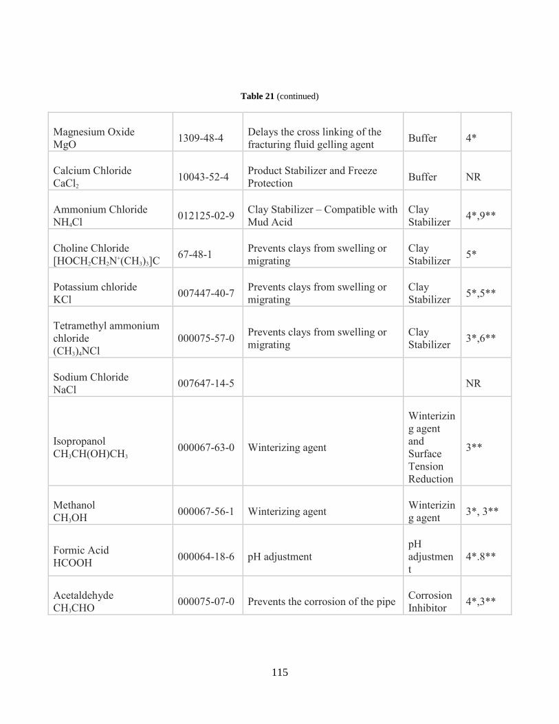
115

Table 21 (continued)

Magnesium Oxide

MgO

1309-48-4

Delays the cross linking of the

fracturing fluid gelling agent

Buffer

4*

Calcium Chloride

CaCl2

10043-52-4

Product Stabilizer and Freeze

Protection

Buffer

NR

Ammonium Chloride

NH4Cl

012125-02-9

Clay Stabilizer – Compatible with

Mud Acid

Clay

Stabilizer

4*,9**

Choline Chloride

[HOCH2CH2N+(CH3)3]C

67-48-1

Prevents clays from swelling or

migrating

Clay

Stabilizer

5*

Potassium chloride

KCl

007447-40-7

Prevents clays from swelling or

migrating

Clay

Stabilizer

5*,5**

Tetramethyl ammonium

chloride

(CH3)4NCl

000075-57-0

Prevents clays from swelling or

migrating

Clay

Stabilizer

3*,6**

Sodium Chloride

NaCl

007647-14-5

NR

Isopropanol

CH3CH(OH)CH3

000067-63-0

Winterizing agent

Winterizin

g agent

and

Surface

Tension

Reduction

3**

Methanol

CH3OH

000067-56-1

Winterizing agent

Winterizin

g agent

3*, 3**

Formic Acid

HCOOH

000064-18-6

pH adjustment

pH

adjustmen

t

4*.8**

Acetaldehyde

CH3CHO

000075-07-0

Prevents the corrosion of the pipe

Corrosion

Inhibitor

4*,3**

116

Table 21 (continued)

Hydrotreated Light

Petroleum Distillate

064742-47-8

Carrier fluid for gelling agents,

friction reducers and crosslinkers

Carrier

fluid and

fluid loss

control

3**

Potassium Metaborate

KBO2

013709-94-9

Crosslinker for borate crosslinked

fluids

Crosslinke

r

3*

Triethanolamine (TEA)

N(CH2CH2OH)3

102-71-6

Maintains fluid viscosity as

temperature increases

Fluid

Stabilizer

5*,3**

Sodium Tetraborate

Na2B4O7

001330-43-4

Crosslinker for borate crosslinked

fluids

Crosslinke

r

4*

Boric Acid

H3BO3

13343-35-3

Crosslinker for borate crosslinked

fluids

Crosslinke

r

4*

Chelated Zirconium

Crosslinker for High Temperature

or low pH Fluids

Crosslinke

r

Zirconium oxychloride

ZrCl2O

7699-43-6

Inorganic Clay Stabilizer

Clay

Stabilizer

4*

Ethylene Glycol

OCH2CH2OH

000107-21-1

Product stabilizer and / or

winterizing agent.

Winterizin

g Agent

4*

Methanol

CH3OH

000067-56-1

Surface Tension Reduction and /

or winterizing agent.

Fluid

Recovery

and

Winterizin

g Agent

3*,3**

Ethanol

C2H5OH

000064-17-5

Product stabilizer and / or

winterizing agent.

Fluid

Recovery

and

Winterizin

g Agent

3**

Polyacrylamide

(C3H5NO)n

009003-05-8

“Slicks” the water to minimize

friction

Friction

Reducer

5*

117

Table 21 (continued)

Guar Gum and its

derivatives HPG,

CMHPG

009000-30-0

Thickens the water in order to

suspend the proppant and reduce

friction

Gelling

Agents

NR

Derivatives of cellulose -

HEC, CMHEC

R(n)OCH2COONa

9004-34-6

9004-32-4

Thickens the water in order to

suspend the proppant and reduce

friction

Gelling

Agents

NR

Xanthan gum

11138-66-2

Thickens Acid in order to control

fluid loss

Gelling

Agent

NR

Citric Acid

(HOOCCH2)2C(OH)COO

H

000077-92-9

Prevents precipitation of metal

oxides

Iron

Control

5*,8**

Acetic Acid

CH3COOH

000064-19-7

Prevents precipitation of metal

oxides and pH control

Iron

Control

and pH

Adjustme

nt

4*,8**

Thioglycolic Acid

HSCH2COOH

000068-11-1

Prevents precipitation of metal

oxides

Iron

Control

3*,8**

Sodium Erythorbate

C6H7O6. Na

006381-77-7

Prevents precipitation of metal

oxides

Iron

Control

NR

Lauryl Sulfate and its

Derivatives

C12H25OSO2ONa

000151-21-3

Used to prevent the formation of

emulsions in the reservoir and to

improve fluid recovery

Non-

Emulsifier

and

Surfactant

s

4*

Sodium Hydroxide

NaOH

001310-73-2

Adjusts the pH of fluid to initiate

the effectiveness of other

components, such as crosslinkers

pH

Adjusting

Agent

4*,8**

Potassium Hydroxide

KOH

001310-58-3

Adjusts the pH of fluid to initiate

the effectiveness of other

components, such as crosslinkers

pH

Adjusting

Agent

2*,8**

118

Table 21 (continued)

Sodium Carbonate

Na2CO3

000497-19-8

Adjusts the pH of fluid to

maintains the effectiveness of

other components, such as

crosslinkers

pH

Adjusting

Agent

5*,5**

Potassium Carbonate

K2CO3

000584-08-7

Adjusts the pH of fluid to

maintains the effectiveness of

other components, such as

crosslinkers

pH

Adjusting

Agent

4*

Sodium Acrylate and

Copolymers of

Acrylamide

C3H3O2. Na

007446-81-3

Prevents scale deposits in the pipe

or in the fracture

Scale

Inhibitor

NR

Sodium Polycarboxylate

N/A

Prevents scale deposits in the pipe

Scale

Inhibitor

Phosphonic Acid Salt

N/A

Prevents scale deposits in the pipe

Scale

Inhibitor

Naphthalene

C10H8

000091-20-3

Carrier fluid for the active

surfactant ingredients

Surfactant

3*,4**

Ethylene glycol

monobutyl ether -

EGMBE

C4H9OCH2CH2OH

000111-76-2

Surface Tension Reduction for

Fluid Recovery

Surfactant

4*, 6**

[i] - 1 – Hazard Rating – An attempt made by the author to rate the hazard level associated with

the chemicals in the list. The first number of Hazard Rating with the “*” is the Poison Hazard

and the second number of Hazard Rating with “**” is the transportation Hazard. The Poison

Hazard is defined by the EU/Swiss Poison Class and the transportation Hazard is defined by the

US Department of Transportation (DOT). The appearance of “NR” means that no rating could be

found, and if a substance is present, that chemical was normally non-hazardous.

[ii] - * EU/Swiss Poison Class

119

BIBLIOGRAPHY

Bahadori, A. (2014). Natural Gas Processing : Technology and Engineering Design. Saint

Louis, MO, USA: Gulf Publishing Company.

Barth, J. (2011). Unanswered Questions About the Economic Impact of Gas Drilling in the

Marcellus Shale. Retrieved June 15, 2016, from Earthworks:

https://www.earthworksaction.org/2010summit/Panel2_JannetteBarth.pdf

Cafaro, D. C., & Grossmann, I. E. (2014). Strategic Planning, Design, and Development of the

Shale. Wiley Online Library (wileyonlinelibrary.com).

Campbell, C. (2015). Natural Gas: Bridging the Gap between Fossil Fuels and Renewable

Energy. Retrieved February 28, 2015, from College of Engineering and Applied Science,

University of Colorado Boulder : http://www.colorado.edu/engineering/profile/natural-

gas-bridging-gap-between-fossil-fuels-and-renewable-energy

Chisholm, H. E. (1910). Entry for 'Petroleum'. 1911 Encyclopedia Britanica.

Colorado School of Mines. (2013). About Produced Water. Retrieved May 20, 2016, from The

Produced Water Treatment and Beneficial Use Imformation Center:

http://aqwatec.mines.edu/produced_water/intro/pw/

Considine, T. J., Watson, R., & Blumsack, S. (2011). Pennsylvania Marcellus Natural Gas

Industry: Status, Economic Impact, and Future Potential. The Pennsylvania State

University, Department of Energy and Mineral Engineering.

Constantine, T. J., Watson, R., & Blumsack, S. (2010). The Economic Impacts of the

Pennsylvania Marcellus Shale Natural Gas Play: An Update. State College, PA: The

Pennsylvania State University, College of Earth and Mineral Sciences, Department of

Energy and Mineral Engineering.

Cowden, E. (2015, June 7). Marcellus Shale Coalition. (Fitzgerald, J. T., Iketani, M., Yang, Y.,

Hefley, W. E., Interviewer)

Crawford, T. (2013, April 25). Hydraulic Fracturing: What is Hydraulic Fracturing? Retrieved

March 14, 2015, from Green Plug District: http://greenplug.nu/hydraulic-fracturing-what-

is-hydraulic-fracturing/

120

D'Annunzio, P. (2016, March 10). $4.24M Awarded for Oil and Gas Water Pollution Read

more: http://www.thelegalintelligencer.com/id=1202751897835/424M-Awarded-for-Oil-

and-Gas-Water-Pollution#ixzz4932FBf4l. Retrieved May 18, 2016, from The Legal

Intelligencer: http://www.thelegalintelligencer.com/id=1202751897835/424M-Awarded-

for-Oil-and-Gas-Water-Pollution?slreturn=20160428180915

David, J. E. (2014, May 8). Energy companies lament skills gap as 'crisis' festers. Retrieved June

23, 2016, from CNBC: http://www.cnbc.com/2014/05/07/stry-jobs-oil-and-gas-firms-say-

they-face-skills-gap.html

EIA. (2008). U.S. Natural Gas Pipeline Compressor Stations Illustration. Retrieved May 15,

2015, from Energy Information Administration:

https://www.eia.gov/pub/oil_gas/natural_gas/analysis_publications/ngpipeline/compresso

rMap.html

EIA. (2009, April). Market Centers and Hubs. Retrieved Jan 22, 2016, from EIA:

http://www.eia.gov/pub/oil_gas/natural_gas/analysis_publications/ngpipeline/MarketCent

erHubsMap.html

EIA. (2011). Natural Gas Processing Plants in the United States. Retrieved Apr 20, 2016, from

U.S. Energy Information Administration:

http://www.eia.gov/pub/oil_gas/natural_gas/feature_articles/2010/ngpps2009/

EIA. (2012, January 24). U.S. energy use projected to grow slowly and become less carbon-

intensive. Retrieved February 27, 2016, from EIA:

http://205.254.135.7/todayinenergy/detail.cfm?id=4690

EIA. (2014, June 6). Delivery and Storage of Natural Gas. Retrieved from U.S. Energy

Information Administration:

http://www.eia.gov/energyexplained/index.cfm?page=natural_gas_delivery

EIA. (2015). Annual Energy Outlook 2015. US Energy Information Administration.

EIA. (2015, Dec 15). Energy in Brief. Retrieved Jan 13, 2016, from

http://www.eia.gov/energy_in_brief/article/shale_in_the_united_states.cfm

EIA. (2015, July 28). Factors Affecting Natural Gas Prices. Retrieved Jan 20, 2016, from EIA

Energy Explained:

http://www.eia.gov/energyexplained/index.cfm?page=natural_gas_factors_affecting_pric

es

EIA. (2015). Natural Gas Plant Processing. Retrieved May 20, 2016, from U.S. Energy

Information Administration: http://www.eia.gov/dnav/ng/ng_prod_pp_dcu_nus-

z00_a.htm

121

EIA. (2015, Aug). Natural Gas Spot and Futures Prices (NYMEX). Retrieved Aug 2015, from

U.S. Energy Information Administration:

https://www.eia.gov/dnav/ng/NG_PRI_FUT_S1_D.htm

EIA. (2015, Nov 5). Oil and Petroleum Products. Retrieved Jan 13, 2016, from Energy

Explained: http://www.eia.gov/energyexplained/index.cfm?page=oil_home

EIA. (2015, April 14). The Annual Energy Outlook 2015. Retrieved Jan 20, 2016, from EIA:

http://www.eia.gov/forecasts/aeo/index.cfm

EIA. (2015, August 6). Wholesale Electricity and Natural Gas Market Data. Retrieved August 7,

2015, from US Energy Information Administration:

http://www.eia.gov/electricity/wholesale/

EIA. (2016, Jan 6). Average annual natural gas spot price in 2015 was at lowest level since

1999. Retrieved Jan 22, 2016, from EIA:

http://www.eia.gov/todayinenergy/detail.cfm?id=24412

EIA. (2016, March 11). Crude Oil Production. Retrieved March 17, 2016, from EIA:

http://www.eia.gov/dnav/pet/pet_crd_crpdn_adc_mbbl_a.htm

EIA. (2016, Feb 29). Natural Gas Consumption by End Use. Retrieved Mar 30, 2016, from EIA:

http://www.eia.gov/dnav/ng/ng_cons_sum_dcu_nus_a.htm

EIA. (2016, April 29). Natural Gas Gross Withdrawals and Production. Retrieved May 20,

2016, from The U.S. Energy Information Administration:

http://www.eia.gov/dnav/ng/ng_prod_sum_dc_NUS_MMCF_m.htm

EIA. (2016, Feb 29). Natural Gas Prices. Retrieved Mar 21, 2016, from The U.S. Energy

Information Administration: http://www.eia.gov/dnav/ng/ng_pri_sum_dcu_nus_m.htm

EIA. (2016, Mar 24). State Electricity Profiles. Retrieved Apr 22, 2016, from US Energy

Information Administration: https://www.eia.gov/state/

EIA. (2016, Jan 21). Weekly Natural Gas Storage Report. Retrieved Jan 22, 2016, from EIA:

http://ir.eia.gov/ngs/ngs.html

EPA. (2010). Methane and Nitrous Oxide Emissions from Natural Sources. Washington DC:

U.S. Environmental Protection Agency.

EPA. (2012). Clean Energy—Air Emissions. Retrieved February 26, 2016, from US

Environmental Protection Agency: http://www.epa.gov/cleanenergy/energy-and-

you/affect/air-emissions.html

122

EPA. (2016, May 26). Overview of Greenhouse Gases. Retrieved May 28, 2016, from United

States Enviromental Protection Agency:

https://www3.epa.gov/climatechange/ghgemissions/gases/ch4.html#ref1

EPA. (2016, April 20). The Hydraulic Fracturing Water Cycle. Retrieved May 18, 2016, from

US Environmental Protection Agency: https://www.epa.gov/hfstudy/hydraulic-fracturing-

water-cycle

EPA. (2016, May 26). U.S. Greenhouse Gas Inventory Report: 1990-2014. Retrieved May 28,

2016, from United States Enviromental Protection Agency:

https://www3.epa.gov/climatechange/ghgemissions/usinventoryreport.html

Faraguna, J. (2013). Skills needed to support the UK shale gas revolution. Retrieved June 26,

2016, from HAYS: Recruiting experts worldwide:

https://social.hays.com/2013/07/16/the-uk-shale-gas-revolution/

Fitzgerald, J. T., Iketani, M., Yang, Y., Hefley, W. E., & Rajgopal, J. (2015). Powering PA: A

Case Study of Distributed Power Generation from Marcellus Shale. Technical Report

No. 2015-10-1, University of Pittsburgh, Department of Industrial Engineering,

Pittsburgh.

Gandossi, L. (2013). An overview of hydraulic fracturing and other formation stimulation

technologies for shale gas production. Institute for Energy and Transport, Joint Research

Centre. Luxembourg: Office of the European Union.

Harrison, J. (2008, Oct 31). DAMS: IMPACTS ON SALMON AND STEELHEAD. Retrieved May

13, 2016, from The Northwest Power and Conservation Council:

https://www.nwcouncil.org/history/DamsImpacts

Hefley, W. E., & Seydor, S. M. (2015). Direct Economic Impact of the Value Chain of a

Marcellus Shale Gas Well. In W. E. Hefley, Economics of Unconventional Shale Gas

Development - Case Studies and Impacts. Springer.

Hefley, W. E., Seydor, S. M., Bencho, M. K., Chappel, L., Dizard, M., Hallman, J., Herkt, J.,

Jiang, P. J., Kerec, M., Lampe, F., Lehner, C. L., Wei, T., Birsic, B., Coulter, E., Hatter,

E. M., Jacko, D., Mignogna, S., Park, N., Riley, K., Tawoda, T., Clements, E., Harlovic,

R. (2011). The Economic Impact of the Value Chain of a Marcellus Shale Well.

University of Pittsburgh. Pittsburgh: Joseph M. Katz Graduate School of Business.

IHS Global Insight. (2011). The Economic and Employment Contributions of Shale Gas in the

United States. IHS Global Insight (USA) Inc. Retrieved from

http://anga.us/media/235626/shale-gas-economic-impact-dec-2011.pdf

INGAA. (2015). Compressor Stations . Retrieved from INGAA:

http://www.ingaa.org/cms/129.aspx

123

INGAA. (2016). Metering Stations and Mainline Valves. Retrieved Jan 20, 2016, from INGAA:

http://www.ingaa.org/cms/131.aspx

Li, X., Omara, M., Sullivan, M., Zimmerman, N., Subramanian, R., Robinson, A., & Presto, A.

(2015, December 14). Volatile Organic Compound Emissions from Natural Gas

Facilities in the Denver-Julesburg Basin, the Uintah Basin and the Marcellus Shale.

Retrieved May 28, 2016, from agu.confex.com:

https://agu.confex.com/agu/fm15/mediafile/.../AGU%20poster_2.2.pdf

Li, Z., Zheng, G., Wu, F., Wendt, A., Gonzales, M., Lauvaux, T., . . . Brantley, S. (2016). A Data

Driven Approach to Assess Environmental Impacts of Shale-Gas Development in an Area

of Hydraulic Fracturing. State Park: The Pennsylvania State University.

Lo, C. (2012, November 16). Flexible fossil fuels: bridging the energy gap. Retrieved February

28, 2016, from power-technology.com: http://www.power-

technology.com/features/featureflexible-fossil-fuels-bridging-energy-gap/

Low, T. (2013, June 21). The Crisis Facing Oil and Gas: Finding Skilled Workers in the Face of

Growing Demand. Retrieved June 23, 2016, from OIL + GAS MONITOR:

http://www.oilgasmonitor.com/the-crisis-facing-oil-and-gas-finding-skilled-workers-in-

the-face-of-growing-demand/

Marcellus-shale.us. (2016). GAS DRILLING WASTEWATER. Retrieved June 2, 2016, from

Marcellus-shale.us: http://www.marcellus-shale.us/drilling_wastewater.htm

Mokhatab, S., Poe, W. A., & Mak, J. Y. (2015). Handbook of Natural Gas Transmission and

Processing : Principles and Practices (3rd Edition). Saint Louis, MO, USA: Elsevier

Science.

Momentive. (2012). Fracturing Fluids 101. Retrieved Jan 20, 2016, from Fracline:

http://www.hexionfracline.com/fracturing-fluids-101

Montgomery, C. (2013). Chapter 1: Fracturing Fluids. In A. P. Bunger, J. McLennan, & R.

Jeffrey, Effective and Sustainable Hydraulic Fracturing. InTech, Chapters published May

17, 2013 under CC BY 3.0 license.

Montgomery, C. T., & Smith, M. B. (2010, Dec). Hydraulic Fracturing: History of an Enduring

Technology. Retrieved Jan 14, 2016, from Journal of Petroleum Technology (JPT)

Online: http://www.jptonline.org/index.php?id=481

Nahmias, S., & Olsen, T. L. (2015). Production and Operations Analysis, Seventh Edition. Long

Grove, IL: Waveland Press, Inc.

National Conference of State Legislatures. (2012). Oil and Gas Severance Taxes: States Work to

Alleviate Fiscal Pressures Amid the Natural Gas Boom. Retrieved from National

124

Conference of State Legislatures: http://www.ncsl.org/research/energy/oil-and-gas-

severance-taxes.aspx

NaturalGas.org. (2013, September 20). Natural Gas Distribution. Retrieved from

NaturalGas.org: http://naturalgas.org/naturalgas/distribution/

NaturalGas.org. (2013, September 20). Overview of Natural Gas. Retrieved May 20, 2016, from

NaturalGas.org: http://naturalgas.org/overview/

Oil & Gas IQ. (2014). Oil & Gas Recruitment: The Great Crew Change. Retrieved June 25,

2016, from Oil & Gas IQ: http://www.oilandgasiq.com/strategy-management-and-

information/white-papers/oil-gas-recruitment-the-great-crew-change/

Patzek, T. W., Male, F., & Marder, M. (2013, December 3). Gas production in the Barnett Shale

obeys a simple scaling theory. PNAS, 110(49), 19731-19736.

PennFuture. (2016). Wind energy is the world's fastest growing source of electricity. Retrieved

Februray 28, 2016, from PennFuture:

http://www.pennfuture.org/content.aspx?MenuID=1&SubSectionID=178&SectionID=34

4

Pennsylvania Public Utility Commission. (2015). Act13/Impact Fee Interactive Website.

Retrieved from Pennsylvania Public Utility Commission: https://www.act13-

reporting.puc.pa.gov/Modules/PublicReporting/Overview.aspx

Rabe, B. G., & Hampton, R. L. (2015). Taxing Fracking: The Politics of State Severance Taxes

in the Shale Era. Review of Policy Research, 32(4), 389-412.

Randazzo, N. (2014, September 4). Oil and Gas Jobs in Demand as Companies Seek to Bridge

Skills Gap. Retrieved June 23, 2016, from DrillingInfo: http://info.drillinginfo.com/oil-

and-gas-jobs-demand-skills-gap/

Robbins, P. (2007). Hydropower. Encyclopedia of Environment and Society.

Seydor, S. M., Clements, E., Pantelemonitis, S., Deshpande, V., Canter, J., Evelyn, I.,Keating,

L., Leonzio, A., Gianoutsos, J., Hammond, J., Burcha, G., Chen, C. T., Chen, W.,

Chutani, R., Dabrowka, S., Mamros, L., Pradhan, A., Perez-Hernande, A., Handayani, D.

P., Hornin, K., Pawar, A., Damesimo, P., Grab, B., Hatok, A., Rexrode, Clark, Shanafelt,

R. (2012). Understanding the Marcellus Shale Supply Chain. Pittsburgh, PA: Working

Paper, Katz Graduate School of Business. University of Pittsburgh.

Strah, S. E. (2015). West Penn Power Current Tariff No. 40 with Supp. Nos. 1-3. Reading, PA:

Pennsylvania Power. Retrieved August 6, 2015, from

www.firstenergycorp.com/content/dam/customer/Customer%20Choice/Files/PA/tariffs/P

P-Tariff-36-w-Supp-4.pdf

125

Toland, B. (2010, April 9). Where are all the Marcellus Shale jobs? Retrieved June 15, 2016,

from Pittsburgh Post-Gazette: http://www.post-gazette.com/pg/10099/1048898-28.stm

USFWS. (2016). Why are salmon in trouble? - Dams. Retrieved May 13, 2016, from U.S. Fish

& Wildlife Service: https://www.fws.gov/salmonofthewest/dams.htm

Water & Wastewater International. (2016). SHALE GAS FRACKING: Water Lessons from the

US to Europe. Retrieved June 5, 2016, from Water & Wastewater International:

http://www.waterworld.com/articles/wwi/print/volume-27/issue-2/regional-spotlight-

europe/shale-gas-fracking.html

Watson, T. L. (1910). Granites of the Southeastern Atlantic States. Washington Government

Printing Office.

Wikimarcellus. (2010, April 30). Slickwater. Retrieved Jan 15, 2016, from Wikimarcellus:

http://waytogoto.com/wiki/index.php/Slickwater