A Study of Segmentation and Normalization

for

Iris Recognition Systems

by

Ehsan M. Arvacheh

A thesis

presented to the University of Waterloo

in fulfillment of the

thesis requirement for the degree of

Master of Applied Science

in

Systems Design Engineering

Waterloo, Ontario, Canada, 2006

c©Ehsan M. Arvacheh 2006

I hereby declare that I am the sole author of this thesis. This is a true copy of the thesis,

including any required final revisions, as accepted by my examiners.

I understand that my thesis may be made electronically available to the public.

Ehsan M. Arvacheh

ii

Abstract

Iris recognition systems capture an image from an individual’s eye. The iris in the image

is then segmented and normalized for feature extraction process. The performance of iris

recognition systems highly depends on segmentation and normalization. For instance, even

an effective feature extraction method would not be able to obtain useful information from

an iris image that is not segmented or normalized properly. This thesis is to enhance the

performance of segmentation and normalization processes in iris recognition systems to

increase the overall accuracy.

The previous iris segmentation approaches assume that the boundary of pupil is a circle.

However, according to our observation, circle cannot model this boundary accurately. To

improve the quality of segmentation, a novel active contour is proposed to detect the

irregular boundary of pupil. The method can successfully detect all the pupil boundaries

in the CASIA database [42] and increase the recognition accuracy.

Most previous normalization approaches employ polar coordinate system to transform

iris. Transforming iris into polar coordinates requires a reference point as the polar origin.

Since pupil and limbus are generally non-concentric, there are two natural choices, pupil

center and limbus center. However, their performance differences have not been investi-

gated so far. We also propose a reference point, which is the virtual center of a pupil with

radius equal to zero. We refer this point as the linearly-guessed center. The experiments

demonstrate that the linearly-guessed center provides much better recognition accuracy.

In addition to evaluating the pupil and limbus centers and proposing a new refer-

ence point for normalization, we reformulate the normalization problem as a minimization

problem. The advantage of this formulation is that it is not restricted by the circular

assumption used in the reference point approaches. The experimental results demonstrate

that the proposed method performs better than the reference point approaches.

In addition, previous normalization approaches are based on transforming iris texture

into a fixed-size rectangular block. In fact, the shape and size of normalized iris have

not been investigated in details. In this thesis, we study the size parameter of traditional

approaches and propose a dynamic normalization scheme, which transforms an iris based

on radii of pupil and limbus. The experimental results demonstrate that the dynamic

normalization scheme performs better than the previous approaches.

iii

Acknowledgements

I would like to express my gratitude to my supervisor, Prof. Hamid R.Tizhoosh. In

the course of my master study, he has provided me with helpful ideas, guidance, comments

and criticisms.

Many thanks to Adams Wai-Kin Kong, Ph.D. Candidate at University of Waterloo.

We enjoyed research together. We discussed our ideas with the hope of getting closer to

the truth. I thank him for all his help and encouragements during my master program.

Thank you to my readers, Prof. John S. Zelek and Prof. Kumaraswamy Ponnambalam

for their useful comments on my thesis as well as their support during my time at University

of Waterloo.

I would like to express my appreciation to the Chinese Academy of Sciences’ Institute

of Automation for generously providing the iris database.

I also thank Libor Masek for sharing his work as an open source iris recognition algo-

rithm. I believe his algorithm is useful for researchers who start working in the field.

I sincerely thank Vicky Lawrence, the graduate secretary of Systems Design Depart-

ment, for being helpful all the time.

Finally, I would like to thank my parents and my brother for believing in me and

supporting me along the way. Thank you.

iv

Contents

1 Introduction 1

1.1 Biometric Technology . . . . . . . . . . . . . . . . . . . . . . . . . . . . . . 1

1.2 Iris Recognition . . . . . . . . . . . . . . . . . . . . . . . . . . . . . . . . . 2

1.3 Thesis Objectives . . . . . . . . . . . . . . . . . . . . . . . . . . . . . . . . 4

1.3.1 Segmentation . . . . . . . . . . . . . . . . . . . . . . . . . . . . . . 5

1.3.2 Normalization . . . . . . . . . . . . . . . . . . . . . . . . . . . . . . 5

1.4 Thesis Layout . . . . . . . . . . . . . . . . . . . . . . . . . . . . . . . . . . 6

2 Background 7

2.1 Segmentation . . . . . . . . . . . . . . . . . . . . . . . . . . . . . . . . . . 7

2.1.1 Daugman’s Integro-differential Operator . . . . . . . . . . . . . . . 7

2.1.2 Hough Transform . . . . . . . . . . . . . . . . . . . . . . . . . . . . 8

2.1.3 Discrete Circular Active Contours . . . . . . . . . . . . . . . . . . . 9

2.1.4 Other Segmentation Methods . . . . . . . . . . . . . . . . . . . . . 11

2.1.5 Problem Statement . . . . . . . . . . . . . . . . . . . . . . . . . . . 12

2.2 Normalization . . . . . . . . . . . . . . . . . . . . . . . . . . . . . . . . . . 15

2.2.1 Daugman’s Cartesian to Polar Transform . . . . . . . . . . . . . . . 15

2.2.2 Wildes’ Image Registration . . . . . . . . . . . . . . . . . . . . . . . 18

2.2.3 Non-linear Normalization Model . . . . . . . . . . . . . . . . . . . . 18

2.2.4 Other Normalization Methods . . . . . . . . . . . . . . . . . . . . . 19

2.2.5 Problem Statement . . . . . . . . . . . . . . . . . . . . . . . . . . . 20

2.3 Summary . . . . . . . . . . . . . . . . . . . . . . . . . . . . . . . . . . . . 21

v

3 Proposed Methods 22

3.1 Segmentation . . . . . . . . . . . . . . . . . . . . . . . . . . . . . . . . . . 22

3.1.1 Pupil Detection: Proposed Near-circular Active Contour . . . . . . 22

3.1.2 Eyelid Model: Elliptic Eyelid Contour . . . . . . . . . . . . . . . . 25

3.1.3 Limbus and Eyelids Detection: Iterative Algorithm . . . . . . . . . 26

3.1.4 Eyelash Detection: MAP Classification with Connectivity Criterion 28

3.2 Normalization . . . . . . . . . . . . . . . . . . . . . . . . . . . . . . . . . . 32

3.2.1 Iris Unwrapping: Proposed Contour-Based Model . . . . . . . . . . 32

3.2.2 Iris Normalization: Proposed Dynamic-Size Model . . . . . . . . . . 38

3.3 Summary . . . . . . . . . . . . . . . . . . . . . . . . . . . . . . . . . . . . 39

4 Experimental Results 41

4.1 Segmentation . . . . . . . . . . . . . . . . . . . . . . . . . . . . . . . . . . 41

4.1.1 Pupil Detection . . . . . . . . . . . . . . . . . . . . . . . . . . . . . 41

4.1.2 Eyelid Model . . . . . . . . . . . . . . . . . . . . . . . . . . . . . . 43

4.1.3 Limbus and Eyelids Detection . . . . . . . . . . . . . . . . . . . . . 47

4.1.4 Eyelash Detection . . . . . . . . . . . . . . . . . . . . . . . . . . . . 53

4.2 Normalization . . . . . . . . . . . . . . . . . . . . . . . . . . . . . . . . . . 57

4.2.1 Iris Unwrapping . . . . . . . . . . . . . . . . . . . . . . . . . . . . . 58

4.2.2 Iris Normalization . . . . . . . . . . . . . . . . . . . . . . . . . . . . 62

4.3 Summary . . . . . . . . . . . . . . . . . . . . . . . . . . . . . . . . . . . . 64

5 Conclusions 67

vi

List of Figures

2.1 The internal forces of the Discrete Circular Active Contour . . . . . . . . . 11

2.2 The external forces of the Discrete Circular Active Contour . . . . . . . . . 12

2.3 Near-circular pupils . . . . . . . . . . . . . . . . . . . . . . . . . . . . . . . 13

2.4 Results of the Integro-differential operator over the near-circular pupils . . 14

2.5 The effect of eyelids and eyelashes on the limbus detection . . . . . . . . . 16

2.6 An iris image from CASIA database . . . . . . . . . . . . . . . . . . . . . . 17

2.7 The normalized iris image using the Cartesian to polar transformation . . . 17

2.8 Different number of samples in each radius of an iris . . . . . . . . . . . . . 21

3.1 Internal force over a vertex . . . . . . . . . . . . . . . . . . . . . . . . . . . 23

3.2 Eyelid curve model based on degree of eye openness: Side view. . . . . . . 26

3.3 Eyelid curve model based on degree of eye openness: Front view. . . . . . . 27

3.4 The iterative algorithm for limbus and eyelid detection. . . . . . . . . . . . 29

3.5 The estimated histogram of iris and eyelashes and the MAP threshold. . . 31

3.6 Unwrapping using the limbus center as the reference point. . . . . . . . . . 34

3.7 Unwrapping using the pupil center as the reference point. . . . . . . . . . . 35

3.8 Unwrapping using the linearly-guessed center as the reference point. . . . . 36

3.9 Double-reference method: equivalent to the linearly-guessed center point . 37

3.10 An example of a fixed-size normalization approach. . . . . . . . . . . . . . 39

3.11 The proposed dynamic-size method . . . . . . . . . . . . . . . . . . . . . . 40

4.1 Near-circular active contour with α = 0.3 . . . . . . . . . . . . . . . . . . . 42

4.2 Near-circular active contour with α = 0.7 . . . . . . . . . . . . . . . . . . . 42

4.3 Results of the Integro-differential operator over the near-circular pupils . . 44

vii

4.4 Results of the proposed active contour over the near-circular pupils . . . . 45

4.5 Successful eyelid detection . . . . . . . . . . . . . . . . . . . . . . . . . . . 46

4.6 Unsuccessful eyelid detection: Double eyelid images . . . . . . . . . . . . . 48

4.7 Unsuccessful eyelid detection: Eyelids covered by eyelashes . . . . . . . . . 49

4.8 Unsuccessful eyelid detection: Eyelid contour misalignment . . . . . . . . . 50

4.9 Inaccurate limbus detection affected by the eyelids and eyelashes . . . . . . 51

4.10 Results of the iterative algorithm, 2 iterations . . . . . . . . . . . . . . . . 52

4.11 Eye images from CASIA database . . . . . . . . . . . . . . . . . . . . . . . 54

4.12 Detected eyelashes . . . . . . . . . . . . . . . . . . . . . . . . . . . . . . . 55

4.13 Unsuccessful eyelash detection . . . . . . . . . . . . . . . . . . . . . . . . . 56

4.14 The average d’ with respect to angular resolution . . . . . . . . . . . . . . 58

4.15 The average d’ with respect to radial resolution . . . . . . . . . . . . . . . 59

4.16 The recognition results: from limbus center to pupil center . . . . . . . . . 60

4.17 The comparison of the linearly-guessed center with limbus and pupil . . . . 60

4.18 The comparison of the linearly-guessed center with the minimum distance . 61

4.19 The impact of the active contour and the contour-based unwrapping . . . . 62

4.20 The comparison of the active contour model with the perfect circles . . . . 63

4.21 The recognition results of the fixed-size normalization method . . . . . . . 64

4.22 The recogniton results of the dynamic-size normalization method . . . . . 65

4.23 The comparison of the average d’ of dynamic and fixed methods . . . . . . 65

viii

Chapter 1

Introduction

1.1 Biometric Technology

Biometric technology deals with recognizing the identity of individuals based on their

unique physical or behavioral characteristics [13]. Physical characteristics such as finger-

print, palm print, hand geometry and iris patterns or behavioral characteristics such as

typing pattern and hand-written signature present unique information about a person and

can be used in authentication applications.

The developments in science and technology have made it possible to use biometrics

in applications where it is required to establish or confirm the identity of individuals.

Applications such as passenger control in airports, access control in restricted areas, border

control, database access and financial services are some of the examples where the biometric

technology has been applied for more reliable identification and verification.

In recent years, biometric identity cards and passports have been issued in some coun-

tries based on iris, fingerprint and face recognition technologies to improve border control

process and simplify passenger travel at the airports. In UK and Australia, biometric

passports based on face recognition are being issued [44]. The technology is designed to

automatically take a picture from the passengers and match it to the digitized image stored

in the biometric passports. Recently, US government is also conducting a Registered Trav-

eler Program which uses a combination of fingerprint and iris recognition technology to

speed up the security check process at some airports [45].

1

2

In the filed of financial services, biometric technology has shown a great potential in

offering more comfort to customers while increasing their security. As an example, banking

services and payments based on biometrics are going to be much safer, faster and easier than

the existing methods based on credit and debit cards. Proposed forms of payments such

as pay and touch scheme based on fingerprint or smart cards with stored iris information

on them are examples of such applications. Although there are still some concerns about

using biometrics in the mass consumer applications due to information protection issues,

it is believed that the technology will find its way to be widely used in many different

applications.

Moreover, access control applications such as database access and computer login also

benefit from the new offered technologies. Compared to passwords, biometric technolo-

gies offer more secure and comfortable accessibility and have dealt with problems such as

forgetting or hacking passwords. For instance, the new login method based on combina-

tion of a password with its typing pattern has been an innovative proposal where knowing

the password itself would not be sufficient [4]. The method is based on typing pattern

of a person by measuring the delays between the typing instances, which is a behavioral

characteristic similar to hand written signature. The proposed method has added up the

security of login-based access systems where a limited number of individuals are expected

to have access to the systems.

Overall, the future of biometric technology is believed to be open for more investments

based on the new services it has to offer to the society. A market overview, reported by

the International Biometric Group (IBG), indicates that the biometric industry revenue

is expected to continuously rise from 1,538.9 million USD in 2005 to 5,749.2 million USD

in 2010 [43]. Currently, this market revenue mostly relies on the existing fingerprint tech-

nologies; however, the new technologies based on face recognition, hand geometry and iris

recognition are expected to relatively expand this revenue in near future.

1.2 Iris Recognition

Iris patterns are formed by combined layers of pigmented epithelial cells, muscles for con-

trolling the pupil, stromal layer consisting of connective tissue, blood vessels and an anterior

3

border layer [1], [13]. The physiological complexity of the organ results in the random pat-

terns in iris, which are statistically unique and suitable for biometric measurements [7].

In addition, iris patterns are stable over time and only minor changes happen to them

throughout an individual’s life [3]. It is also an internal organ, located behind the cornea

and aqueous humor, and well protected from the external environment. The characteris-

tics such as being protected from the environment and having more reliable stability over

time, compared to other popular biometrics, have well justified the ongoing research and

investments on iris recognition by various researchers and industries around the world. For

instance, the developed algorithm by Daugman [7], which is known as the state-of-the-art

in the field of iris recognition, has initiated huge investments on the technology for more

than a decade. IriScan Inc. patents the core technology of the Daugman’s system and

several companies such as IBM, Iridian Technologies, IrisGuard Inc., Securimetrics Inc.

and Panasonic are active in providing iris recognition products and services.

The history of iris recognition goes back to mid 19th-century when the French physician,

Alphonse Bertillon, studied the use of eye color as an identifier [2]. However, it is believed

that the main idea of using iris patterns for identification, the way we know it today, was

first introduced by an eye surgeon, Frank Burch, in 1936 [6]. In 1987, two ophthalmologists,

Flom and Safir, patented this idea [3] and proposed it to Daugman, a professor at Harvard

University, to study the possibility of developing an iris recognition algorithm. After a

few years of scientific experiments, Daugman proposed and developed a high confidence

iris recognition system and published the results in 1993 [7]. The proposed system then

evolved and achieved better performance in time by testing and optimizing it with respect

to large iris databases.

The reports have shown that Daugman’s system has zero false match rate based on

the tests done by organizations such as British Telecom, US Sandia Labs, UK National

Physical Laboratory, The National Biometric Test Center of SJSU, EyeTicket, Siemens,

Unisys, LG, IriScan, Iridian, Sensar, and Sarno [9]. The information extracted from an

iris is in binary format and it is stored in only 256 bytes to allow creation of nationwide

IrisCode databases. The search engine is based on Boolean exclusive-OR operator (XOR)

to allow extremely fast comparisons in the matching process. Moreover, the degrees-of-

freedom of an IrisCode template, which indicates the statistical complexity of an iris based

4

on the entropy theory of Shannon [5], is about 249. The number of degrees-of-freedom of

the iris templates shows that the complexity of iris patterns is relatively high compared

to other biometric measures. The overall characteristics of the proposed algorithm offers

real-time and high confidence identification in applications such as passenger control in

airports, border control and access control in high-security areas. Currently, Daugman’s

iris recognition system is installed in several airports worldwide. Noteworthy to mention is

the currently installed system in the United Arabs Emirates that is capable of identifying

individuals within 2 seconds and performs about 2 billion comparisons daily.

A few years after the publication of the first algorithm by Daugman, other researchers

developed new iris recognition algorithms. Systems presented by Wildes et al. [11], Boles

and Boashash [14], Tisse et al. [16], Zhu et al. [17], Lim et al. [18], Noh et al. [19] and Ma

et al. [20] are some of the well-known algorithms so far. Among these algorithms, the works

done by Lim et al. and Noh et al. are also commercialized. The algorithms developed

by Wildes and Boles are suitable for verification applications because the normalization of

irises is performed in the matching process and would be very time consuming in identifi-

cation applications. Although these algorithms have been successful, they still require to

be improved in the accuracy and speed aspects compared to the proposed algorithm by

Daugman.

Although Daugman’s algorithm can perform fast and accurate recognition of irises,

some details about the algorithm are not published. For instance, normalizing iris based

on polar transformation requires a proper reference point as the polar origin. However, the

details on this reference point have not been discussed. In this thesis, segmentation and

normalization of iris is studied. The previous works on segmentation and normalization

are evaluated and compared. Moreover, new segmentation and normalization methods are

proposed that improve the recognition performance.

1.3 Thesis Objectives

The overall performance of an iris recognition system relies on the performance of its sub-

systems. The qualities of the image acquisition, segmentation, normalization and feature

extraction, altogether, define the performance of the system. For instance, Lim reports

5

an 88.2% success rate over 6,000 iris images in the preprocessing stage due to undesired

factors such as occlusion of irises by eyelids, shadow of eyelids and noises within pupils.

Such degradation of the preprocessing stage could be considered as the degradation of the

overall performance of the system.

1.3.1 Segmentation

Properly detecting the inner and outer boundaries of iris texture is significantly impor-

tant in all iris recognition systems. All the previous segmentation techniques model iris

boundaries and the two eyelids with simple geometric models. Pupil and limbus are often

modeled as circles and the two eyelids are modeled as parabolic arcs. However, according

to our observation, circle cannot model pupil boundary effectively. Irregular boundary of

pupil is the motivation to create an accurate pupil detection algorithm based on the con-

cept of active contours. The contour model takes into consideration that an actual pupil

boundary is a near-circular contour rather than a perfect circle. The objective of this work

is to demonstrate that this method can effectively improve the recognition accuracy.

1.3.2 Normalization

The next focus of this work is on iris normalization. Most normalization techniques are

based on transforming iris into polar coordinates, known as unwrapping process. Pupil

boundary and limbus boundary are generally two non-concentric contours. The non-

concentric condition leads to different choices of reference points for transforming an iris

into polar coordinates. Proper choice of reference point is very important where the radial

and angular information would be defined with respect to this point.

In the experiments, first, the performance of several reference points are examined

including pupil center, limbus center and the linearly-guessed center point. Unwrapping

iris using pupil center is proposed by Lim [18] and Boles [15]. The linearly-guessed center

is equivalent to the technique used by Joung [32]. The objective of the experiments is to

illustrate the step-by-step improvements of the recognition results when the unwrapping

reference point moves toward the linearly-guessed center point starting from the limbus

center. Moreover, a contour-based unwrapping method is designed based on the assumption

6

that iris textures would not tend to be in excessive radial tension from pupil boundary to

limbus boundary. This method reformulates the normalization problem as a minimization

problem. The experimental results demonstrate that the proposed method performs better

than the reference point approaches.

In addition, most normalization approaches based on Cartesian to polar transformation

unwrap the iris texture into a fixed-size rectangular block. As an example, in Lim’s method,

after finding the center of pupil and the inner and outer boundaries of iris, the texture is

transformed into polar coordinates with a fixed resolution. In the radial direction, the

texture is normalized from the inner boundary to the outer boundary into 60 pixels. The

angular resolution is also fixed to a 0.8◦ over the 360◦, which produces 450 pixels in the

angular direction. Other researchers such as Tisse et al., Boles et al. and Ma et al.

also use the fixed size polar transformation model. This technique seems to be useful

in bringing iris images into a standard form, which would simplify the feature extraction

process. However, the circular shape of an iris implies that there are different number of

pixels over each radius. Transforming information of different radii into same resolution

results in different amount of interpolations, and sometimes loss of information, which may

degrade the performance of the system. In this thesis, we investigate the size parameter

of the fixed-size approach. Moreover, a new normalization technique is proposed which

takes into account that iris textures have different number of pixels over each radius. The

polar resolution of irises is then dynamically adjusted with respect to the number pixels in

each radius. The experimental results demonstrate that the dynamic normalization scheme

performs better than the fixed-size approach.

1.4 Thesis Layout

The rest of the thesis is organized as follows. Chapter 2 is background review of some well-

known segmentation and normalization methods. In chapter 3, the proposed methods for

improving segmentation and normalization are presented. Chapter 4 is the experimental

results for illustrating the improvements of the proposed segmentation and normalization

methods on the recognition performance. Chapter 5 offers concluding remarks and points

out the contributions of this thesis.

Chapter 2

Background

2.1 Segmentation

In segmentation, it is desired to distinguish the iris texture from the rest of the image. An

iris is normally segmented by detecting its inner (pupil) and outer (limbus) boundaries.

Well-known methods such as the Integro-differential, Hough transform and active contour

models have been successful techniques in detecting the boundaries. In the following, these

methods are described and some of their weaknesses are pointed out.

2.1.1 Daugman’s Integro-differential Operator

In order to localize an iris, Daugman proposed the Integro-differential operator [7]. The

operator assumes that pupil and limbus are circular contours and performs as a circular

edge detector. Detecting the upper and lower eyelids are also performed using the Integro-

differential operator by adjusting the contour search from circular to a designed arcuate

[9]. The Integro-differential is defined as:

max(r, x0, y0)

∣∣∣∣∣Gσ(r) ∗ ∂

∂r

∫

(r,x0,y0)

I(x, y)2πr

ds

∣∣∣∣∣. (2.1)

The operator pixel-wise searches throughout the raw input image, I(x, y), and obtains

the blurred partial derivative of the integral over normalized circular contours in different

7

8

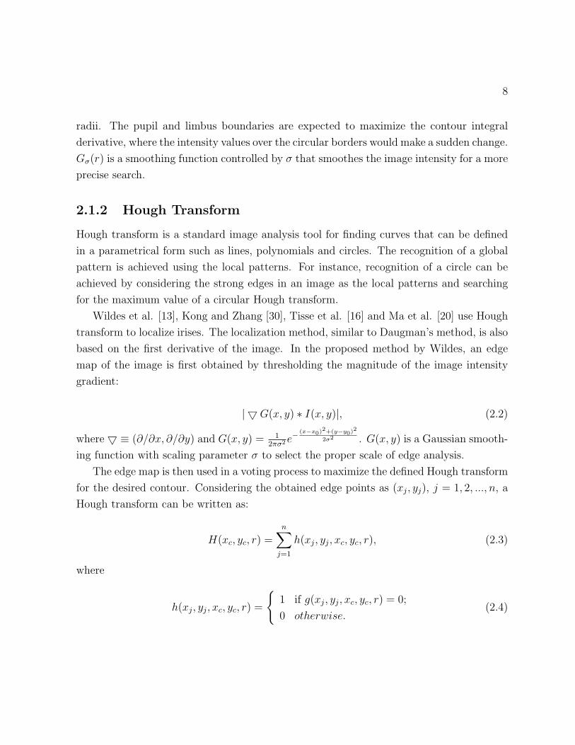
radii. The pupil and limbus boundaries are expected to maximize the contour integral

derivative, where the intensity values over the circular borders would make a sudden change.

Gσ(r) is a smoothing function controlled by σ that smoothes the image intensity for a more

precise search.

2.1.2 Hough Transform

Hough transform is a standard image analysis tool for finding curves that can be defined

in a parametrical form such as lines, polynomials and circles. The recognition of a global

pattern is achieved using the local patterns. For instance, recognition of a circle can be

achieved by considering the strong edges in an image as the local patterns and searching

for the maximum value of a circular Hough transform.

Wildes et al. [13], Kong and Zhang [30], Tisse et al. [16] and Ma et al. [20] use Hough

transform to localize irises. The localization method, similar to Daugman’s method, is also

based on the first derivative of the image. In the proposed method by Wildes, an edge

map of the image is first obtained by thresholding the magnitude of the image intensity

gradient:

| 5G(x, y) ∗ I(x, y)|, (2.2)

where 5 ≡ (∂/∂x, ∂/∂y) and G(x, y) = 12πσ2 e

− (x−x0)2+(y−y0)2

2σ2 . G(x, y) is a Gaussian smooth-

ing function with scaling parameter σ to select the proper scale of edge analysis.

The edge map is then used in a voting process to maximize the defined Hough transform

for the desired contour. Considering the obtained edge points as (xj, yj), j = 1, 2, ..., n, a

Hough transform can be written as:

H(xc, yc, r) =n∑

j=1

h(xj, yj, xc, yc, r), (2.3)

where

h(xj, yj, xc, yc, r) =

{1 if g(xj, yj, xc, yc, r) = 0;

0 otherwise.(2.4)

9

The limbus and pupil are both modeled as circles and the parametric function g is

defined as:

g(xj, yj, xc, yc, r) = (xj − xc)2 + (yj − yc)

2 − r2. (2.5)

Assuming a circle with the center (xc, yc) and radius r, the edge points that are located

over the circle result in a zero value of the function. The value of g is then transformed to 1

by the h function, which represents the local pattern of the contour. The local patterns are

then used in a voting procedure using the Hough transform, H, in order to locate the proper

pupil and limbus boundaries. In order to detect limbus, only vertical edge information is

used. The upper and lower parts, which have the horizontal edge information, are usually

covered by the two eyelids. The horizontal edge information is used for detecting the upper

and lower eyelids, which are modeled as parabolic arcs.

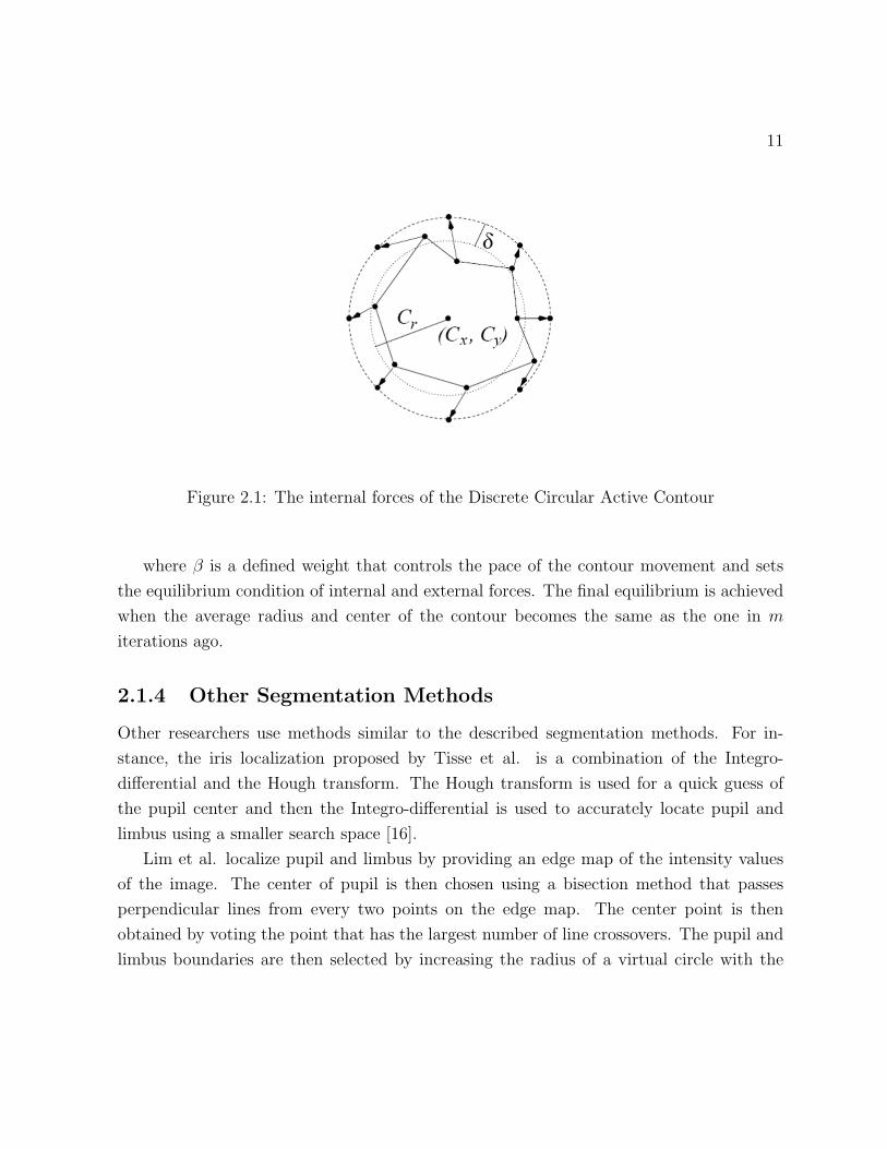
2.1.3 Discrete Circular Active Contours

Ritter proposed an active contour model to localize iris in an image [36]. The model detects

pupil and limbus by activating and controlling the active contour using two defined forces:

internal and external forces. The internal forces are responsible to expand the contour into

a perfect polygon with a radius δ larger than the contour average radius. The internal

force, Fint,i, applied to each vertex, Vi, is defined as:

Fint,i = Vi − Vi, (2.6)

where Vi is the expected position of the vertex in the perfect polygon. The position of

Vi can be obtained with respect to Cr, the average radius of the current contour, and the

contour center, C = (Cx, Cy). The center of a contour is defined as:

C = (xC , yC) =1

n

n∑i=1

Vi, (2.7)

which is the average position of all contour vertices. The average radius of the contour is

defined as:

10

Cr =1

n

n∑i=1

‖Vi − C‖, (2.8)

which is the average distance of all the vertices from the defined center point. The position

of the vertices of the expected perfect polygon is then obtained as:

Vi = (Cx + (Cr + δ)cos(2πi/n), Cy + (Cr + δ)sin(2πi/n)), (2.9)

where n is the total number of vertices.

The internal forces are designed to expand the contour and keep it circular. The force

model assumes that pupil and limbus are globally circular, rather than locally, to minimize

the undesired deformations due to specular reflections and dark patches near the pupil

boundary.

The contour detection process of the model is based on the equilibrium of the defined

internal forces with the external forces. The external forces are obtained from the grey level

intensity values of the image and are designed to push the vertices inward. The magnitude

of the external forces is defined as:

‖Fext,i‖ = I(Vi)− I(Vi + Fext,i), (2.10)

where I(Vi) is the grey level value of the nearest neighbor to Vi. Fext,i is the direction of

the external force for each vertex and it is defined as a unit vector given by:

Fext,i =C − Vi

‖C − Vi‖ . (2.11)

Therefore, the external force over each vertex can be written as:

Fext,i = ‖Fext,i‖Fext,i. (2.12)

The movement of the contour is based on the composition of the internal and external

forces over the contour vertices. Replacement of each vertex is obtained iteratively by:

Vi(t + 1) = Vi(t) + βFint,i + (1− β)Fext,i, (2.13)

11

Figure 2.1: The internal forces of the Discrete Circular Active Contour

where β is a defined weight that controls the pace of the contour movement and sets

the equilibrium condition of internal and external forces. The final equilibrium is achieved

when the average radius and center of the contour becomes the same as the one in m

iterations ago.

2.1.4 Other Segmentation Methods

Other researchers use methods similar to the described segmentation methods. For in-

stance, the iris localization proposed by Tisse et al. is a combination of the Integro-

differential and the Hough transform. The Hough transform is used for a quick guess of

the pupil center and then the Integro-differential is used to accurately locate pupil and

limbus using a smaller search space [16].

Lim et al. localize pupil and limbus by providing an edge map of the intensity values

of the image. The center of pupil is then chosen using a bisection method that passes

perpendicular lines from every two points on the edge map. The center point is then

obtained by voting the point that has the largest number of line crossovers. The pupil and

limbus boundaries are then selected by increasing the radius of a virtual circle with the

12

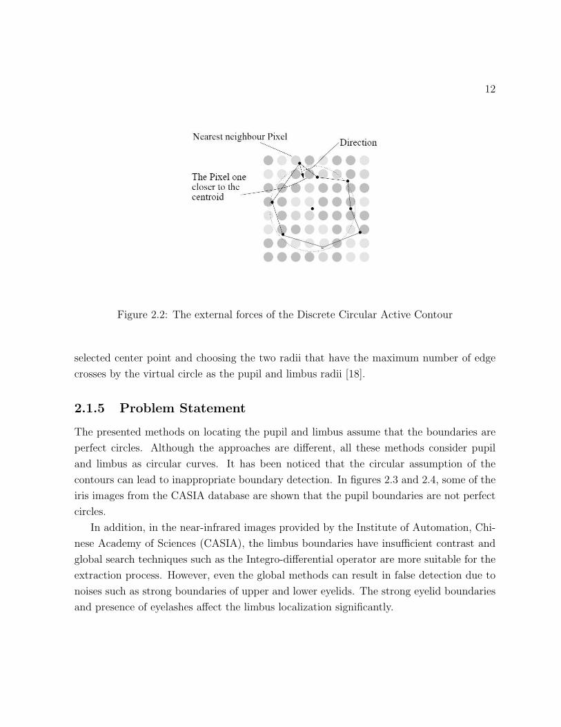
Figure 2.2: The external forces of the Discrete Circular Active Contour

selected center point and choosing the two radii that have the maximum number of edge

crosses by the virtual circle as the pupil and limbus radii [18].

2.1.5 Problem Statement

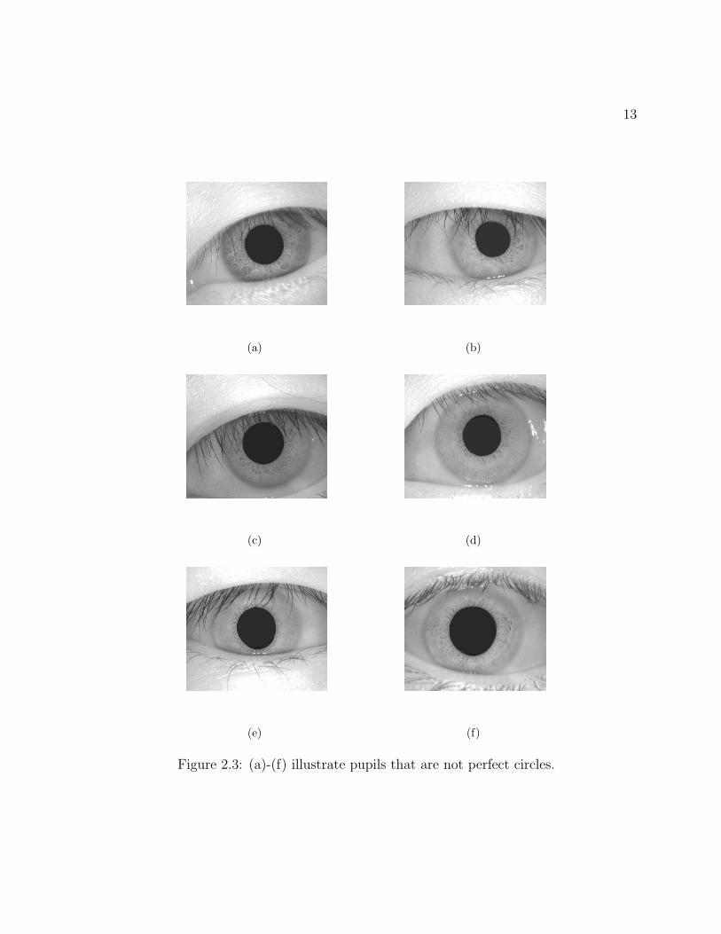
The presented methods on locating the pupil and limbus assume that the boundaries are

perfect circles. Although the approaches are different, all these methods consider pupil

and limbus as circular curves. It has been noticed that the circular assumption of the

contours can lead to inappropriate boundary detection. In figures 2.3 and 2.4, some of the

iris images from the CASIA database are shown that the pupil boundaries are not perfect

circles.

In addition, in the near-infrared images provided by the Institute of Automation, Chi-

nese Academy of Sciences (CASIA), the limbus boundaries have insufficient contrast and

global search techniques such as the Integro-differential operator are more suitable for the

extraction process. However, even the global methods can result in false detection due to

noises such as strong boundaries of upper and lower eyelids. The strong eyelid boundaries

and presence of eyelashes affect the limbus localization significantly.

13

(a) (b)

(c) (d)

(e) (f)

Figure 2.3: (a)-(f) illustrate pupils that are not perfect circles.

14

(a) (b)

(c) (d)

(e) (f)

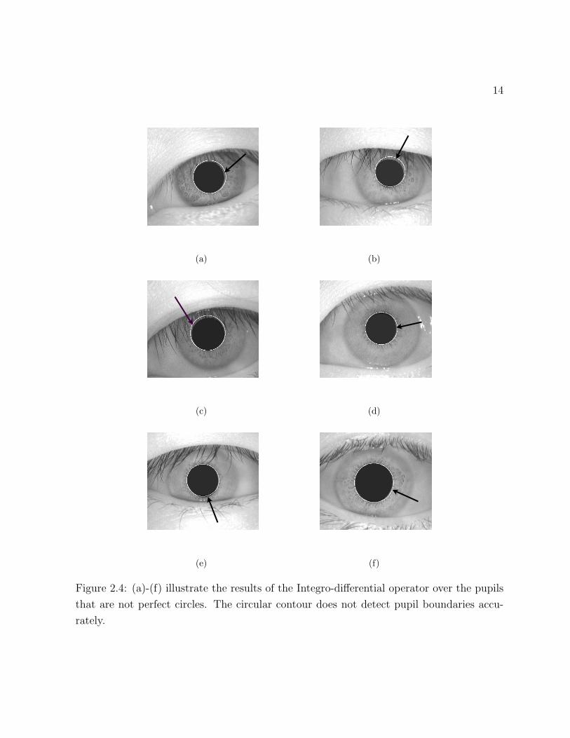
Figure 2.4: (a)-(f) illustrate the results of the Integro-differential operator over the pupils

that are not perfect circles. The circular contour does not detect pupil boundaries accu-

rately.

15

Figure 2.5 shows some of the cases where the presence of eyelids and eyelashes have

affected the localization process.

2.2 Normalization

Normalization refers to preparing a segmented iris image for the feature extraction process.

In Cartesian coordinates, iris images are highly affected by their distance and angular

position with respect to the camera. Moreover, illumination has a direct impact on pupil

size and causes non-linear variations of the iris patterns. A proper normalization technique

is expected to transform the iris image to compensate these variations.

2.2.1 Daugman’s Cartesian to Polar Transform

Daugman’s normalization method transforms a localized iris texture from Cartesian to po-

lar coordinates. The proposed method is capable of compensating the unwanted variations

due to distance of eye from camera (scale) and its position with respect to the camera

(translation). The Cartesian to polar transform is defined as:

x(ρ, θ) = (1− ρ)× xp(θ) + ρ× xi(θ),y(ρ, θ) = (1− ρ)× yp(θ) + ρ× yi(θ),

where

xp(θ) = xp0(θ) + rp × cos(θ),

yp(θ) = yp0(θ) + rp × sin(θ),

xi(θ) = xi0(θ) + ri × cos(θ),

yi(θ) = yi0(θ) + ri × sin(θ).

The process is inherently dimensionless in the angular direction. In the radial direction,

the texture is assumed to change linearly, which is known as the rubber sheet model. The

rubber sheet model linearly maps the iris texture in the radial direction from pupil border

to limbus border into the interval [0 1] and creates a dimensionless transformation in the

radial direction as well.

16

(a) (b)

(c) (d)

(e) (f)

Figure 2.5: (a)-(f) illustrate the inaccurate results of limbus detection because of low

contrast of limbus and presence of eyelids and eyelashes.

17

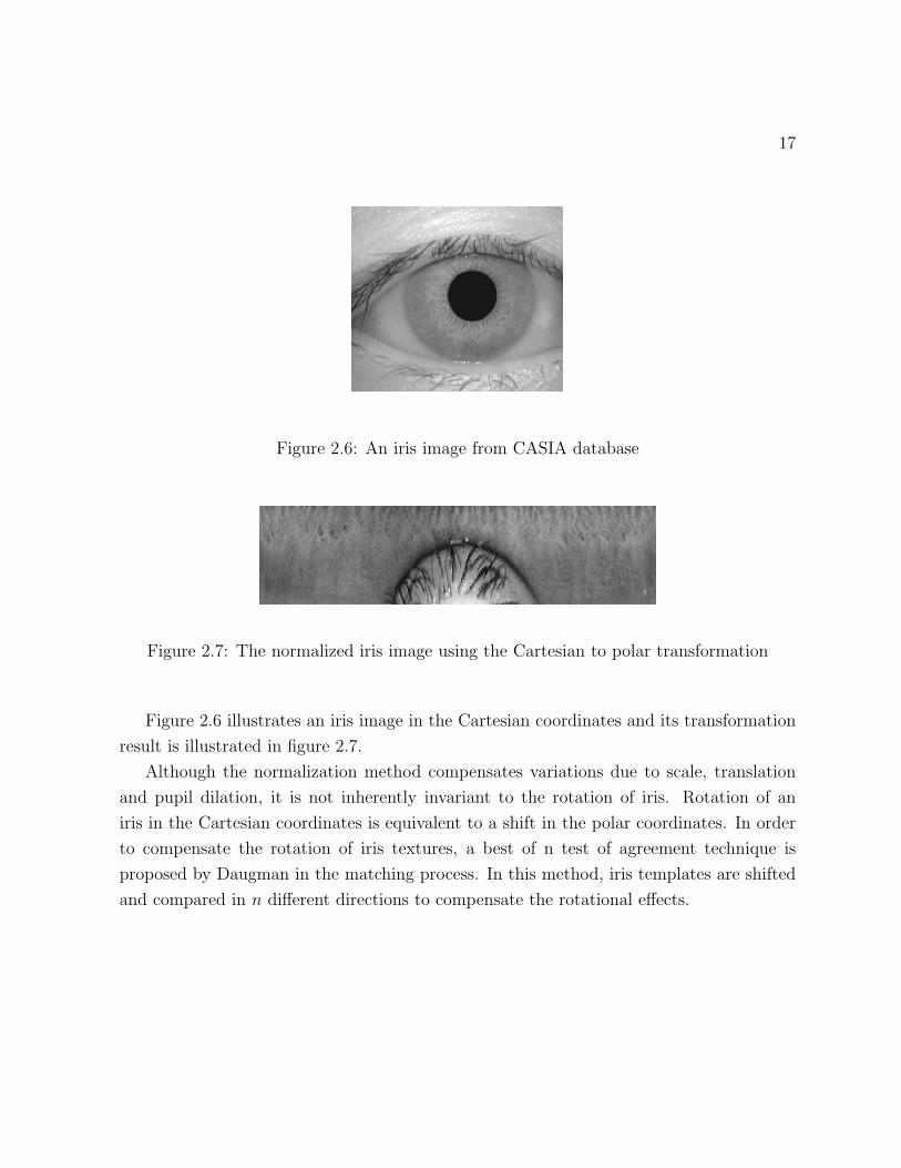
Figure 2.6: An iris image from CASIA database

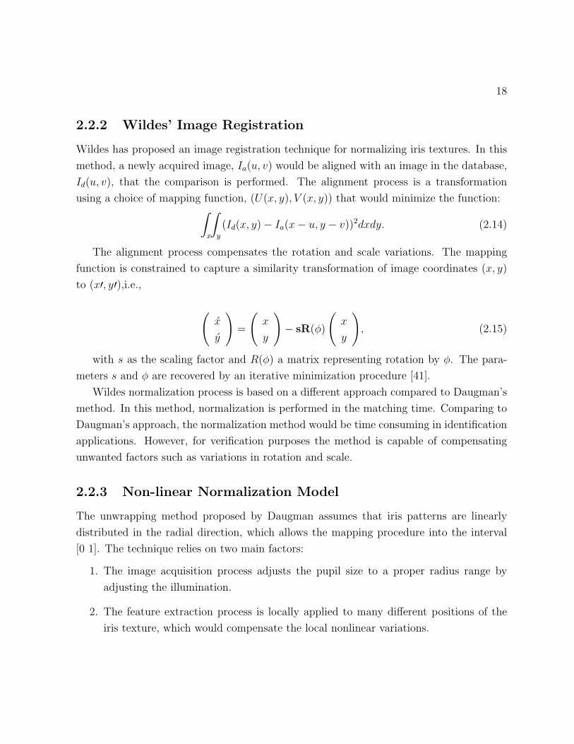
Figure 2.7: The normalized iris image using the Cartesian to polar transformation

Figure 2.6 illustrates an iris image in the Cartesian coordinates and its transformation

result is illustrated in figure 2.7.

Although the normalization method compensates variations due to scale, translation

and pupil dilation, it is not inherently invariant to the rotation of iris. Rotation of an

iris in the Cartesian coordinates is equivalent to a shift in the polar coordinates. In order

to compensate the rotation of iris textures, a best of n test of agreement technique is

proposed by Daugman in the matching process. In this method, iris templates are shifted

and compared in n different directions to compensate the rotational effects.

18

2.2.2 Wildes’ Image Registration

Wildes has proposed an image registration technique for normalizing iris textures. In this

method, a newly acquired image, Ia(u, v) would be aligned with an image in the database,

Id(u, v), that the comparison is performed. The alignment process is a transformation

using a choice of mapping function, (U(x, y), V (x, y)) that would minimize the function:∫

x

∫

y

(Id(x, y)− Ia(x− u, y − v))2dxdy. (2.14)

The alignment process compensates the rotation and scale variations. The mapping

function is constrained to capture a similarity transformation of image coordinates (x, y)

to (x′, y′),i.e.,

(x

y

)=

(x

y

)− sR(φ)

(x

y

), (2.15)

with s as the scaling factor and R(φ) a matrix representing rotation by φ. The para-

meters s and φ are recovered by an iterative minimization procedure [41].

Wildes normalization process is based on a different approach compared to Daugman’s

method. In this method, normalization is performed in the matching time. Comparing to

Daugman’s approach, the normalization method would be time consuming in identification

applications. However, for verification purposes the method is capable of compensating

unwanted factors such as variations in rotation and scale.

2.2.3 Non-linear Normalization Model

The unwrapping method proposed by Daugman assumes that iris patterns are linearly

distributed in the radial direction, which allows the mapping procedure into the interval

[0 1]. The technique relies on two main factors:

1. The image acquisition process adjusts the pupil size to a proper radius range by

adjusting the illumination.

2. The feature extraction process is locally applied to many different positions of the

iris texture, which would compensate the local nonlinear variations.

19

The proposed non-linear normalization method proposed by Yuan and Shi [33], consid-

ers a nonlinear behavior of iris patterns due to changes of pupil size. In order to unwrap

an iris region properly, a non-linear model and a linear normalization model are com-

bined. The non-linear method, which is first applied to an iris image, is based on three

assumptions:

1. The pupil margin and iris root (which correspond to the inner and outer boundaries

of the iris) are concentric circles.

2. The margin of the pupil does not rotate significantly during pupil size changes.

3. The pupil shape does not change and remain circular when pupil size changes.

The non-linear model is defined by virtual arcs, which are named ”fibers” following

Wyatts work, that connect a point on the pupil border to a point on the limbus [34]. The

polar angle traversed by the arcs between these two points is Π/2. The virtual arcs are

defined based on normalized pupil sizes to a fixed value using a pre-defined λref , which is

obtained by the mean of all λ values defined as λ = r/R in the iris database. The r and

R represent the radius of pupil and limbus respectively. The reference annular zone with

λref is then linearly mapped into a fixed-size rectangle zone of m× n by equally sampling

m points in each virtual concentric sampling circle with a fixed radial resolution.

It is concluded by the authors of the presented approach that the non-linear model still

simplifies the real physiological mechanism of iris deformation and some more assumptions

and approximations are required to support the model. The model is also believed to

explicitly show the non-linear behavior of iris textures due to the improvements obtained

in the experiments.

2.2.4 Other Normalization Methods

Lim et al. uses a method very similar to the pseudo polar transform of Daugman. In

this method, after finding the center of pupil and the inner and outer boundaries of iris,

the texture is transformed into polar coordinates with a fixed resolution. In the radial

direction, the texture is normalized from the inner boundary to the outer boundary into

20

60 pixels which is fixed throughout all iris images. The angular resolution is also fixed to

a 0.8 degree over the 360 degree which produces 450 pixels in the angular direction.

Boles’ normalization technique is also similar to Daugman’s method with the difference

that it is performed at the time of matching. The method is based on the diameter of the

two matching irises. The ratio of the diameters are calculated and the diameter of irises

are adjusted to have the same diameters. The number of samples is also fixed and it is set

to a power-of-two integer in order to be suitable for the dyadic wavelet transform.

In addition, there has been some research on the pseudo polar transform in order to

optimize its performance. The work presented by Joung et al. [32] discusses the different

possibilities of iris transformation. The research focuses on the fact that pupil and limbus

are not always concentric and presents a method to improve the unwrapping process [32].

2.2.5 Problem Statement

Most of the normalization methods used in the proposed algorithms transform iris images

from Cartesian to polar coordinates. This technique is efficient in the sense that the nor-

malization process is performed prior to the matching time and is suitable for identification

applications.

Although the normalization process proposed by Daugman has shown to be efficient,

there are some aspects that are required to be investigated and discussed in details. The

proposed pseudo polar transform is known to map an iris texture into the interval [0 1]

in the radial direction . Moreover, in the original formulation of the transformation, each

point over the iris texture is presented by a polar coordinate (r, θ). However, the question

arises by the fact that pupil and limbus are not always concentric and the definition of

polar coordinates requires a center point as the polar origin.

Some works such as the algorithms presented by Boles or Lim et al. unwrap the texture

based on pupil center. A more recent research presented by Joung et al. uses an unwrapping

method that improves the alignment of irises [32]. In this method, it is suggested to use

limbus center to define the polar coordinates of the points over the limbus boundary and to

use pupil center to define the polar coordinates of the pupil boundary. The coordinates of

the other points between the two borders are then obtained linearly in the radial direction.

In addition, most normalization methods based on the Cartesian to polar transforma-

21

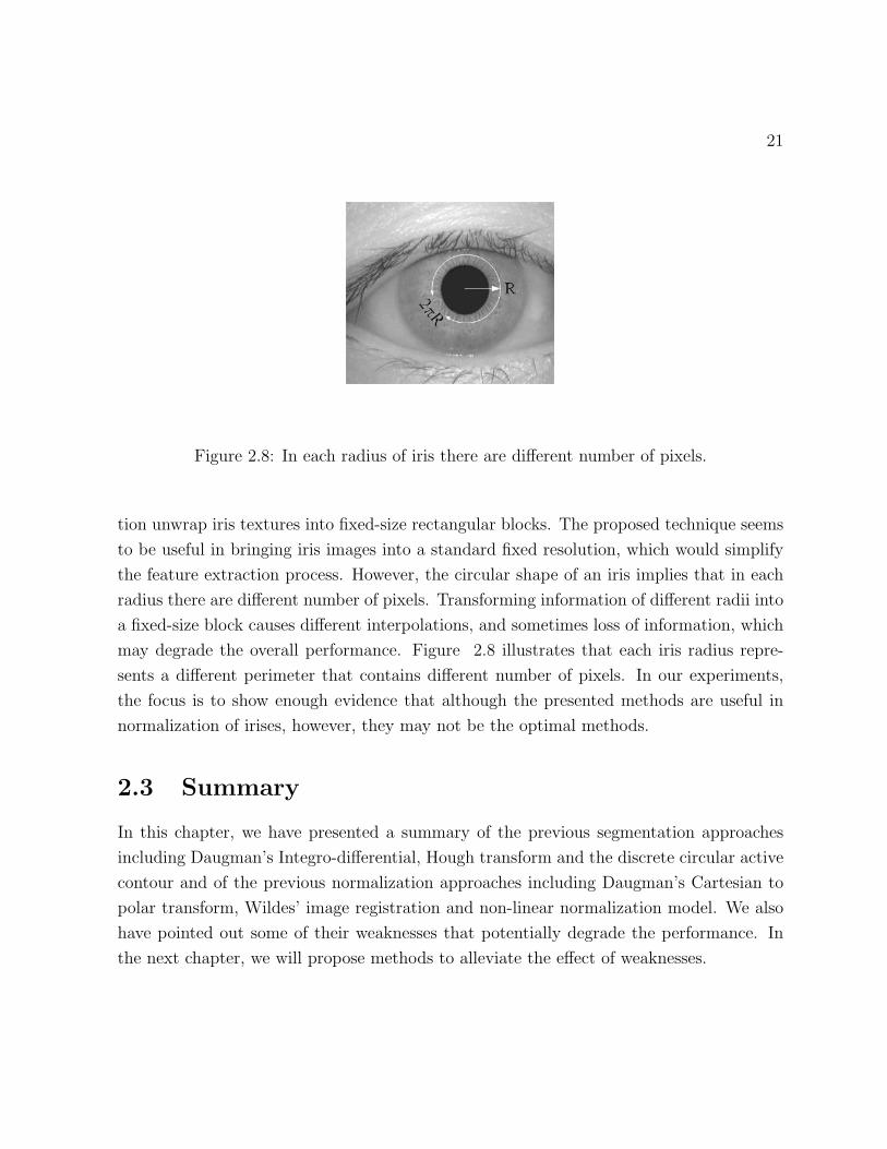
Figure 2.8: In each radius of iris there are different number of pixels.

tion unwrap iris textures into fixed-size rectangular blocks. The proposed technique seems

to be useful in bringing iris images into a standard fixed resolution, which would simplify

the feature extraction process. However, the circular shape of an iris implies that in each

radius there are different number of pixels. Transforming information of different radii into

a fixed-size block causes different interpolations, and sometimes loss of information, which

may degrade the overall performance. Figure 2.8 illustrates that each iris radius repre-

sents a different perimeter that contains different number of pixels. In our experiments,

the focus is to show enough evidence that although the presented methods are useful in

normalization of irises, however, they may not be the optimal methods.

2.3 Summary

In this chapter, we have presented a summary of the previous segmentation approaches

including Daugman’s Integro-differential, Hough transform and the discrete circular active

contour and of the previous normalization approaches including Daugman’s Cartesian to

polar transform, Wildes’ image registration and non-linear normalization model. We also

have pointed out some of their weaknesses that potentially degrade the performance. In

the next chapter, we will propose methods to alleviate the effect of weaknesses.

Chapter 3

Proposed Methods

3.1 Segmentation

3.1.1 Pupil Detection: Proposed Near-circular Active Contour

In order to effectively extract a pupil boundary, it is essential to define the contour char-

acteristics that the system aims to capture. In general, a pupil boundary is a closed,

continuous and smooth curve, which is near-circular. In order to achieve a better perfor-

mance in the next stages of an iris recognition system, it is essential to capture this contour

with respect to a proper center point and a proper angular resolution. The center point of

the contour is defined as the mean of the vertices, which can be written as:

C = (xC , yC) =1

N

N∑i=1

Vi, (3.1)

where N is the total number of vertices and Vi is the ith vertex.

The angular resolution of the contour is another important aspect that should be con-

sidered. The continuity criterion is defined based on the angular resolution rather than

the distance between the vertices which is common in general active contour models [38].

This resolution is chosen based on the average radius of pupils in the database of eye im-

ages. Considering the average radius of 45 pixels, the perimeter of a circle has around 285

pixels. In this case, a resolution of 400 angles is chosen in order to obtain contours that

22

23

are pixel-wise continuous. The number of vertices is constant and each vertex represents a

specific angle throughout the process. This condition can be considered as angular forces

that bring the vertices in the right angular position with respect to the updated contour

center.

Each vertex of a contour is represented by a vector, which has a specific radius and

direction with respect to the center point. In order to obtain a smooth curve with a near-

circular shape, the internal forces are applied in the radial direction in a way to make

the neighboring vertices have the same radius value in a proper angular range, ∆θ. The

magnitude of an internal force applied to a single vertex is defined as:

|Fint,i| = 1

N∆θ

×

θk=θi+∆θ2∑

θk=θi−∆θ2

Rθk

−Ri, (3.2)

where ∆θ represents the angular range, N∆θ represents the number of vertices in the defined

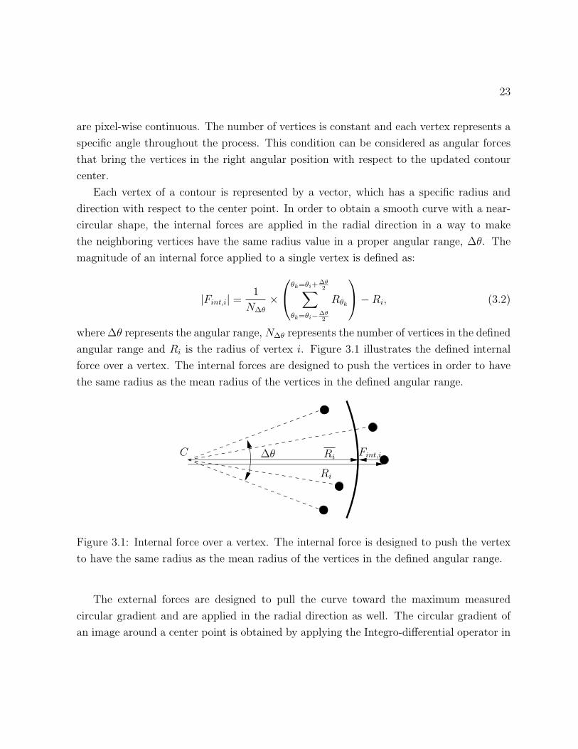
angular range and Ri is the radius of vertex i. Figure 3.1 illustrates the defined internal

force over a vertex. The internal forces are designed to push the vertices in order to have

the same radius as the mean radius of the vertices in the defined angular range.

C ∆θ Ri

Ri

Fint,i

Figure 3.1: Internal force over a vertex. The internal force is designed to push the vertex

to have the same radius as the mean radius of the vertices in the defined angular range.

The external forces are designed to pull the curve toward the maximum measured

circular gradient and are applied in the radial direction as well. The circular gradient of

an image around a center point is obtained by applying the Integro-differential operator in

24

different angles with the proper angular range, ∆θ. The Daugman’s Integro-differential is

basically a circular edge detector, which is defined as:

argmax(r,x0,y0)

∣∣∣∣∣Gσ(r) ∗ ∂

∂r

∫

(r,x0,y0)

I(x, y)2πr

ds

∣∣∣∣∣. (3.3)

The original formulation of the Integro-differential integrates over the interval [0, 2π],

which is a complete circle. However, the definition of the external forces are based on

obtaining the circular edge information in a smaller angular range. Our experiments show

that an angular range of ∆θ = π10

can be a proper value in order to obtain both the internal

and external forces for the near-circular assumption of the pupil boundaries. The external

forces are then defined by the radial distance of each vertex from the maximum circular

gradient and can be written as:

|Fext,i| = argmax(RC)

∣∣∣∣∣∂

∂r

∫ θi+∆θ2

θi−∆θ2

I(x, y)2πr

ds

∣∣∣∣∣−Ri. (3.4)

The proposed external forces which are based on gathering gradient information in

the radial directions have the advantage that the contour would not stop in a local ridge

or valley and the possibility of missing the pupil becomes very low. The search for the

pupil boundary for obtaining the internal and external forces is performed by considering

a search interval around the median value of the obtained radial information of pupil in

the previous iteration. This technique increases the speed of the algorithm by limiting the

search space and filters out the external forces that are pointing out to strong edges such

as eyelids and eyelashes instead of the pupil boundary. In addition, in order to make the

algorithm faster, the external forces are calculated in only 128 angular directions and the

rest of the values would be interpolated based on the near-circular assumption of the pupil

boundary in the angular range ∆θ = π10

.

The radial movement of the contour is based on composition of the internal and external

forces over the contour vertices and the replacement of each vertex in the radial direction

is obtained iteratively by:

RVi(n + 1) = RVi

(n) + Fint,i + α× Fext,i, (3.5)

25

where RViis the radius of vertex i and α ∈ (0, 1) is a weight which controls the pace

of contour movement and sets the equilibrium condition of internal and external forces.

Smaller values of α result in smoother contours, however the contour moves toward the

maximum gradient area in a slower pace. Increasing α increases the effect of external forces

and the contour vertices move toward the pupil boundary in a faster pace. The value of

α should be smaller than 1 to converge to the pupil boundary. If α is greater than 1, the

contour would oscillate near the pupil boundary due to definition of the external forces.

The final equilibrium is reached when the average radius and center of the contour become

the same as the ones in the previous iteration.

In this process, there are fixed number of vertices. Each vertex represents a specific

angle throughout the iterations with respect to the updated contour center. This condition

can be considered as angular forces that are responsible for readjusting the angular position

of the vertices with respect to the updated center point.

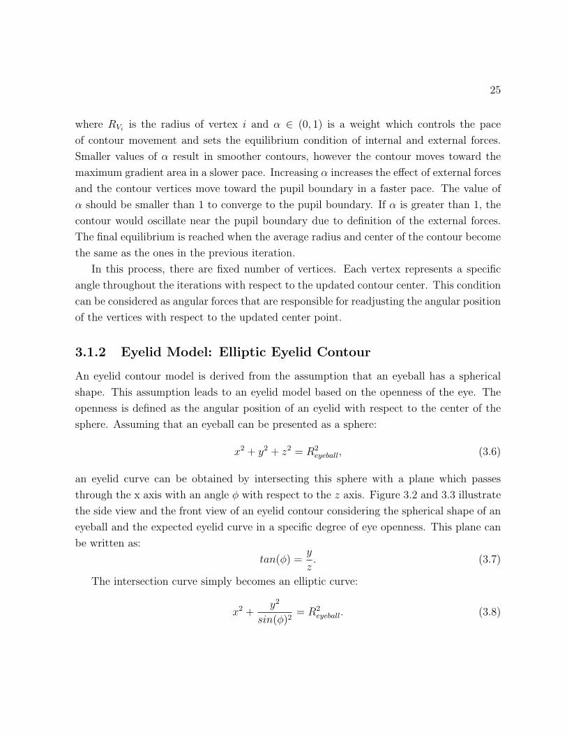
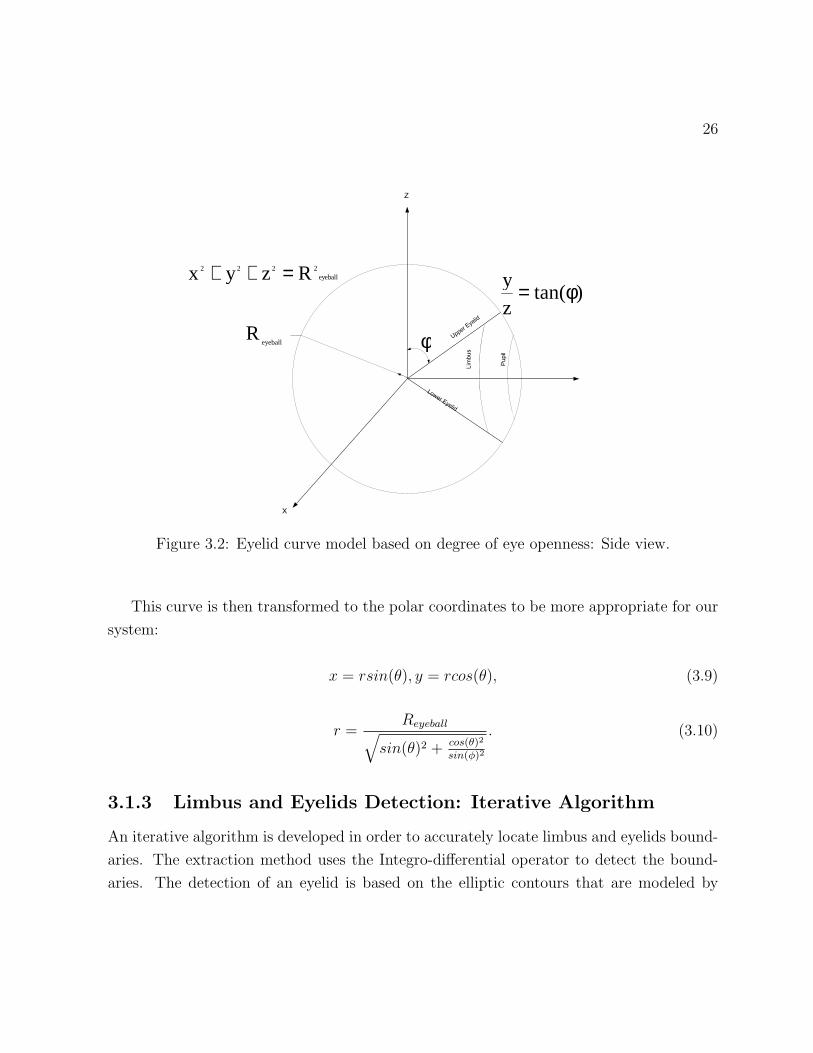
3.1.2 Eyelid Model: Elliptic Eyelid Contour

An eyelid contour model is derived from the assumption that an eyeball has a spherical

shape. This assumption leads to an eyelid model based on the openness of the eye. The

openness is defined as the angular position of an eyelid with respect to the center of the

sphere. Assuming that an eyeball can be presented as a sphere:

x2 + y2 + z2 = R2eyeball, (3.6)

an eyelid curve can be obtained by intersecting this sphere with a plane which passes

through the x axis with an angle φ with respect to the z axis. Figure 3.2 and 3.3 illustrate

the side view and the front view of an eyelid contour considering the spherical shape of an

eyeball and the expected eyelid curve in a specific degree of eye openness. This plane can

be written as:

tan(φ) =y

z. (3.7)

The intersection curve simply becomes an elliptic curve:

x2 +y2

sin(φ)2= R2

eyeball. (3.8)

26

�

�

)tan(zy φ=

φ

eyeball2222 Rzyx =++

eyeballR ��

��������

���������

����

�����

Figure 3.2: Eyelid curve model based on degree of eye openness: Side view.

This curve is then transformed to the polar coordinates to be more appropriate for our

system:

x = rsin(θ), y = rcos(θ), (3.9)

r =Reyeball√

sin(θ)2 + cos(θ)2

sin(φ)2

. (3.10)

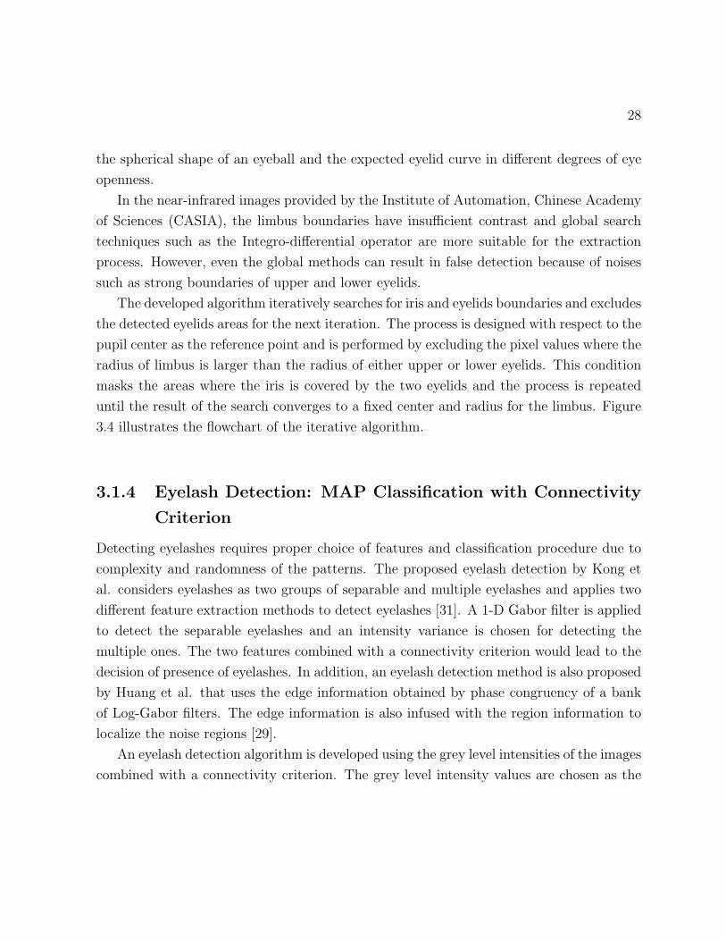
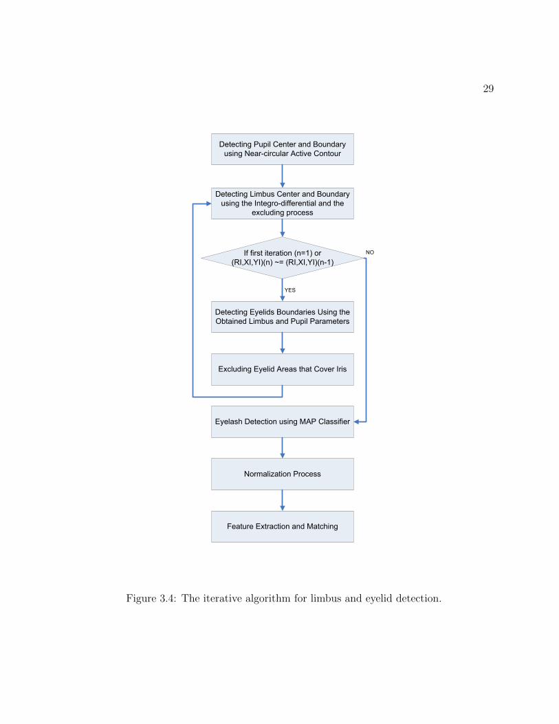
3.1.3 Limbus and Eyelids Detection: Iterative Algorithm

An iterative algorithm is developed in order to accurately locate limbus and eyelids bound-

aries. The extraction method uses the Integro-differential operator to detect the bound-

aries. The detection of an eyelid is based on the elliptic contours that are modeled by

27

�

eyeball2

2

2

2 R)(sin

yx =

φ+

�

eyeballR

���������

� ���� ���

��� ���� ���

Figure 3.3: Eyelid curve model based on degree of eye openness: Front view.

28

the spherical shape of an eyeball and the expected eyelid curve in different degrees of eye

openness.

In the near-infrared images provided by the Institute of Automation, Chinese Academy

of Sciences (CASIA), the limbus boundaries have insufficient contrast and global search

techniques such as the Integro-differential operator are more suitable for the extraction

process. However, even the global methods can result in false detection because of noises

such as strong boundaries of upper and lower eyelids.

The developed algorithm iteratively searches for iris and eyelids boundaries and excludes

the detected eyelids areas for the next iteration. The process is designed with respect to the

pupil center as the reference point and is performed by excluding the pixel values where the

radius of limbus is larger than the radius of either upper or lower eyelids. This condition

masks the areas where the iris is covered by the two eyelids and the process is repeated

until the result of the search converges to a fixed center and radius for the limbus. Figure

3.4 illustrates the flowchart of the iterative algorithm.

3.1.4 Eyelash Detection: MAP Classification with Connectivity

Criterion

Detecting eyelashes requires proper choice of features and classification procedure due to

complexity and randomness of the patterns. The proposed eyelash detection by Kong et

al. considers eyelashes as two groups of separable and multiple eyelashes and applies two

different feature extraction methods to detect eyelashes [31]. A 1-D Gabor filter is applied

to detect the separable eyelashes and an intensity variance is chosen for detecting the

multiple ones. The two features combined with a connectivity criterion would lead to the

decision of presence of eyelashes. In addition, an eyelash detection method is also proposed

by Huang et al. that uses the edge information obtained by phase congruency of a bank

of Log-Gabor filters. The edge information is also infused with the region information to

localize the noise regions [29].

An eyelash detection algorithm is developed using the grey level intensities of the images

combined with a connectivity criterion. The grey level intensity values are chosen as the

29

�������������� ������������������

������������������������� �����

����������������������������

��� !� "������#����� !� "�������

����������$�%&�� ������������������

������'����������������������������'��

�(��������������

����������)�����������������*������'��

+&�������$�%&�������������%������

)(�������)�������������'��� ���������

)�����'����������������,�� ���������

���%���-������������

.������)(�������������,���'���

")/

�+

Figure 3.4: The iterative algorithm for limbus and eyelid detection.

30

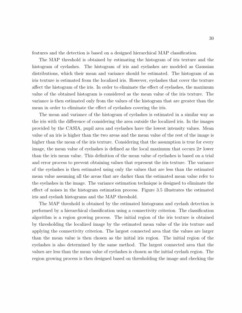
features and the detection is based on a designed hierarchical MAP classification.

The MAP threshold is obtained by estimating the histogram of iris texture and the

histogram of eyelashes. The histogram of iris and eyelashes are modeled as Gaussian

distributions, which their mean and variance should be estimated. The histogram of an

iris texture is estimated from the localized iris. However, eyelashes that cover the texture

affect the histogram of the iris. In order to eliminate the effect of eyelashes, the maximum

value of the obtained histogram is considered as the mean value of the iris texture. The

variance is then estimated only from the values of the histogram that are greater than the

mean in order to eliminate the effect of eyelashes covering the iris.

The mean and variance of the histogram of eyelashes is estimated in a similar way as

the iris with the difference of considering the area outside the localized iris. In the images

provided by the CASIA, pupil area and eyelashes have the lowest intensity values. Mean

value of an iris is higher than the two areas and the mean value of the rest of the image is

higher than the mean of the iris texture. Considering that the assumption is true for every

image, the mean value of eyelashes is defined as the local maximum that occurs 2σ lower

than the iris mean value. This definition of the mean value of eyelashes is based on a trial

and error process to prevent obtaining values that represent the iris texture. The variance

of the eyelashes is then estimated using only the values that are less than the estimated

mean value assuming all the areas that are darker than the estimated mean value refer to

the eyelashes in the image. The variance estimation technique is designed to eliminate the

effect of noises in the histogram estimation process. Figure 3.5 illustrates the estimated

iris and eyelash histograms and the MAP threshold.

The MAP threshold is obtained by the estimated histograms and eyelash detection is

performed by a hierarchical classification using a connectivity criterion. The classification

algorithm is a region growing process. The initial region of the iris texture is obtained

by thresholding the localized image by the estimated mean value of the iris texture and

applying the connectivity criterion. The largest connected area that the values are larger

than the mean value is then chosen as the initial iris region. The initial region of the

eyelashes is also determined by the same method. The largest connected area that the

values are less than the mean value of eyelashes is chosen as the initial eyelash region. The

region growing process is then designed based on thresholding the image and checking the

31

IrisµEyelash

µ��������

��� ���

������������

��� ���

IrisσEyelash

σ

θ

Figure 3.5: The estimated histogram of iris and eyelashes and the MAP threshold.

32

connectivity criterion in a way that the classification of the two regions would reach and

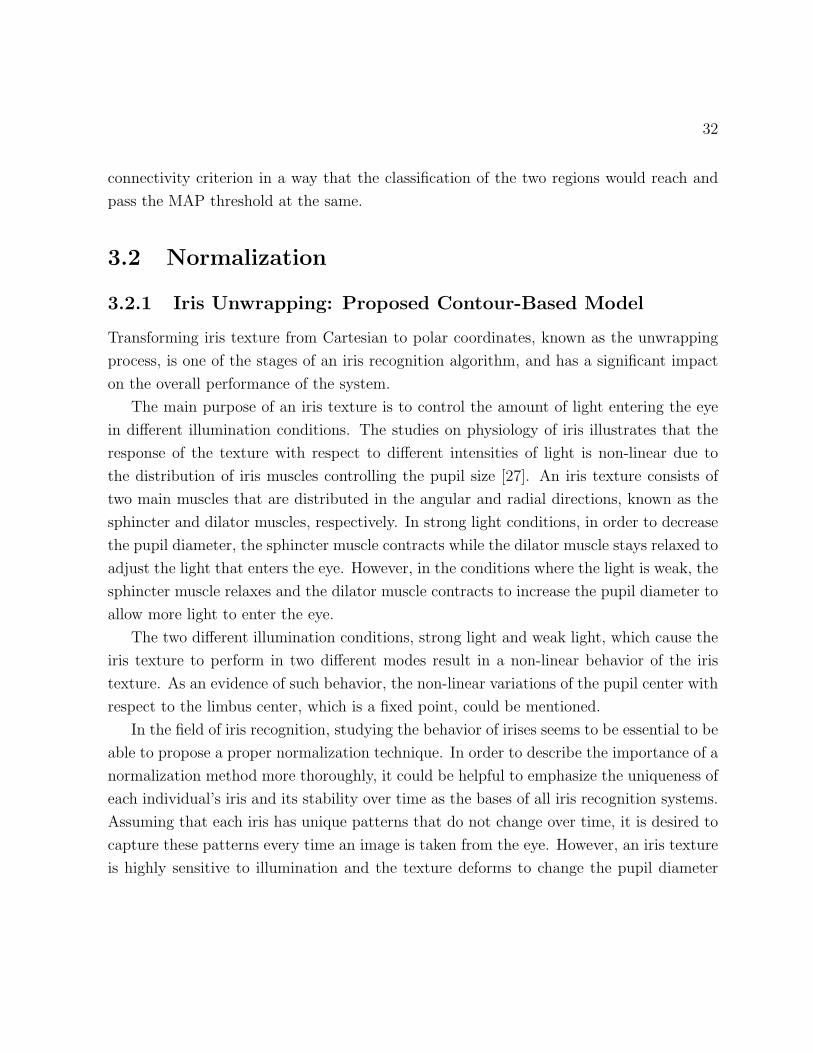
pass the MAP threshold at the same.

3.2 Normalization

3.2.1 Iris Unwrapping: Proposed Contour-Based Model

Transforming iris texture from Cartesian to polar coordinates, known as the unwrapping

process, is one of the stages of an iris recognition algorithm, and has a significant impact

on the overall performance of the system.

The main purpose of an iris texture is to control the amount of light entering the eye

in different illumination conditions. The studies on physiology of iris illustrates that the

response of the texture with respect to different intensities of light is non-linear due to

the distribution of iris muscles controlling the pupil size [27]. An iris texture consists of

two main muscles that are distributed in the angular and radial directions, known as the

sphincter and dilator muscles, respectively. In strong light conditions, in order to decrease

the pupil diameter, the sphincter muscle contracts while the dilator muscle stays relaxed to

adjust the light that enters the eye. However, in the conditions where the light is weak, the

sphincter muscle relaxes and the dilator muscle contracts to increase the pupil diameter to

allow more light to enter the eye.

The two different illumination conditions, strong light and weak light, which cause the

iris texture to perform in two different modes result in a non-linear behavior of the iris

texture. As an evidence of such behavior, the non-linear variations of the pupil center with

respect to the limbus center, which is a fixed point, could be mentioned.

In the field of iris recognition, studying the behavior of irises seems to be essential to be

able to propose a proper normalization technique. In order to describe the importance of a

normalization method more thoroughly, it could be helpful to emphasize the uniqueness of

each individual’s iris and its stability over time as the bases of all iris recognition systems.

Assuming that each iris has unique patterns that do not change over time, it is desired to

capture these patterns every time an image is taken from the eye. However, an iris texture

is highly sensitive to illumination and the texture deforms to change the pupil diameter

33

and control the amount of light entering the eye. The deformation of the texture also

results in the deformation of the iris patterns. In other words, the iris patterns change due

to different illumination conditions. In order to obtain the unique patterns of the iris, it is

desired to be able to track the changes of the iris to recover the unique patterns.

It should be mentioned that the way an iris responses to illumination also varies from

eye to eye due to different distributions of the muscles controlling the pupil. Therefore,

it seems more practical to study the behavior of a large number of irises to obtain a

normalization model that is optimal in capturing and tracking the patterns. In this thesis,

different normalization methods are examined over irises in the CASIA database in order

to find an optimal normalization technique.

Limbus Center: the Unwrapping Reference Point

The limbus center of an iris can be used as the reference point to unwrap the iris texture.

The possible advantage of this point is that limbus contour is fixed and does not change

over time. Figure 3.6 shows an unwrapping method using limbus center as the reference

point.

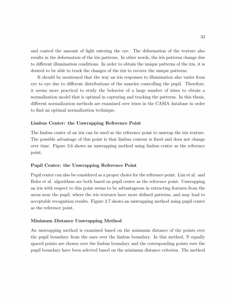
Pupil Center: the Unwrapping Reference Point

Pupil center can also be considered as a proper choice for the reference point. Lim et al. and

Boles et al. algorithms are both based on pupil center as the reference point. Unwrapping

an iris with respect to this point seems to be advantageous in extracting features from the

areas near the pupil, where the iris textures have more defined patterns, and may lead to

acceptable recognition results. Figure 3.7 shows an unwrapping method using pupil center

as the reference point.

Minimum Distance Unwrapping Method

An unwrapping method is examined based on the minimum distance of the points over

the pupil boundary from the ones over the limbus boundary. In this method, N equally

spaced points are chosen over the limbus boundary and the corresponding points over the

pupil boundary have been selected based on the minimum distance criterion. The method

34

���������������

�������������

�

Figure 3.6: Unwrapping using the limbus center as the reference point.

results in global and local minimum distance between the points over the two boundaries.

It should be noticed that the minimum distance method can cause irregular resolution over

the pupil boundary due to different positioning of the pupil center with respect to limbus

center.

In addition, the experiments have been repeated for the condition where N equally

spaced points are chosen over the pupil boundary instead of the limbus boundary to con-

sider their potential differences.

Contour-Based Method: Global Minimum

Similar to the minimum distance method, an unwrapping method is studied based on the

global minimum of the distances between the limbus and pupil boundaries. In this method,

spite of the minimum distance method, the points that are chosen over both of the borders

are equally spaced and the positioning of the two borders are based on their global distance.

The global minimum distance of the contour-based model is defined as:

35

���������������

������������� �

Figure 3.7: Unwrapping using the pupil center as the reference point.

argmin(xp(θo),yp(θo))

(

∫ 2π

0

√((xi − xp(θ))2 + (yi − yp(θ))2)d(θ)), (3.11)

where (xi, yi) and (xp, yp) are the limbus and pupil borders respectively. θo is defined as the

angular offset for the pupil border in order to minimize the global minimum formulation.

The initial idea of both the minimum distance and the contour-based methods have

arisen from the assumption that an iris texture tends to be in its most relaxed state in each

pupil diameter. Therefore, it would make sense to adjust the points over the two borders

in a way that the texture would not be in excessive radial tension. Moreover, both the

minimum distance and the contour-based models have the advantage over the center based

techniques in cases where the pupils are not perfectly circular. In cases where the pupil

borders are not perfect circles and have been detected by the active contour model, center-

based models may not be as robust as contour based models with due to the sensitivity of

the normalization to the correct choice of center point.

36

���������������

�������������

���� ����� ����� �

Figure 3.8: Unwrapping using the linearly-guessed center as the reference point.

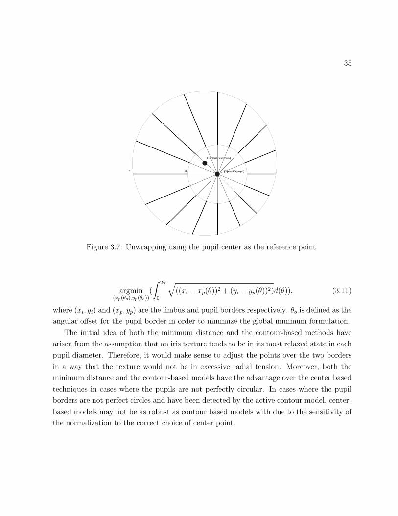
Linearly-Guessed Reference Point Method

In addition to the center-based models based on limbus and pupil centers, the performance

of a linearly-guessed center point is also examined. In this method, the reference point is

obtained by a linear estimation using centers and radii of pupil and limbus. Figure 3.8

illustrates the method for positioning the reference point. This method suggests that the

unwrapping process should be performed by a point that the pupil center tends to reach

when the pupil radius approaches to zero. The limbus center and radius are considered

as the starting state and the pupil center and radius are considered as a measurement in

order to linearly guess the the position of the pupil center when its radius is zero.

It should be mentioned that the linearly-guessed center point is equivalent to the un-

wrapping method presented by Joung [32]. Figure 3.9 illustrates the equivalence of the

linearly-guessed method with the method based on unwrapping an iris with respect to both

limbus and pupil centers.

37

���������������

�������������

���� ����� ����

�

�

�������

������

�

��

�

��

Figure 3.9: Double-reference method used by Joung is equivalent to the proposed linearly-

guessed center point.

38

3.2.2 Iris Normalization: Proposed Dynamic-Size Model

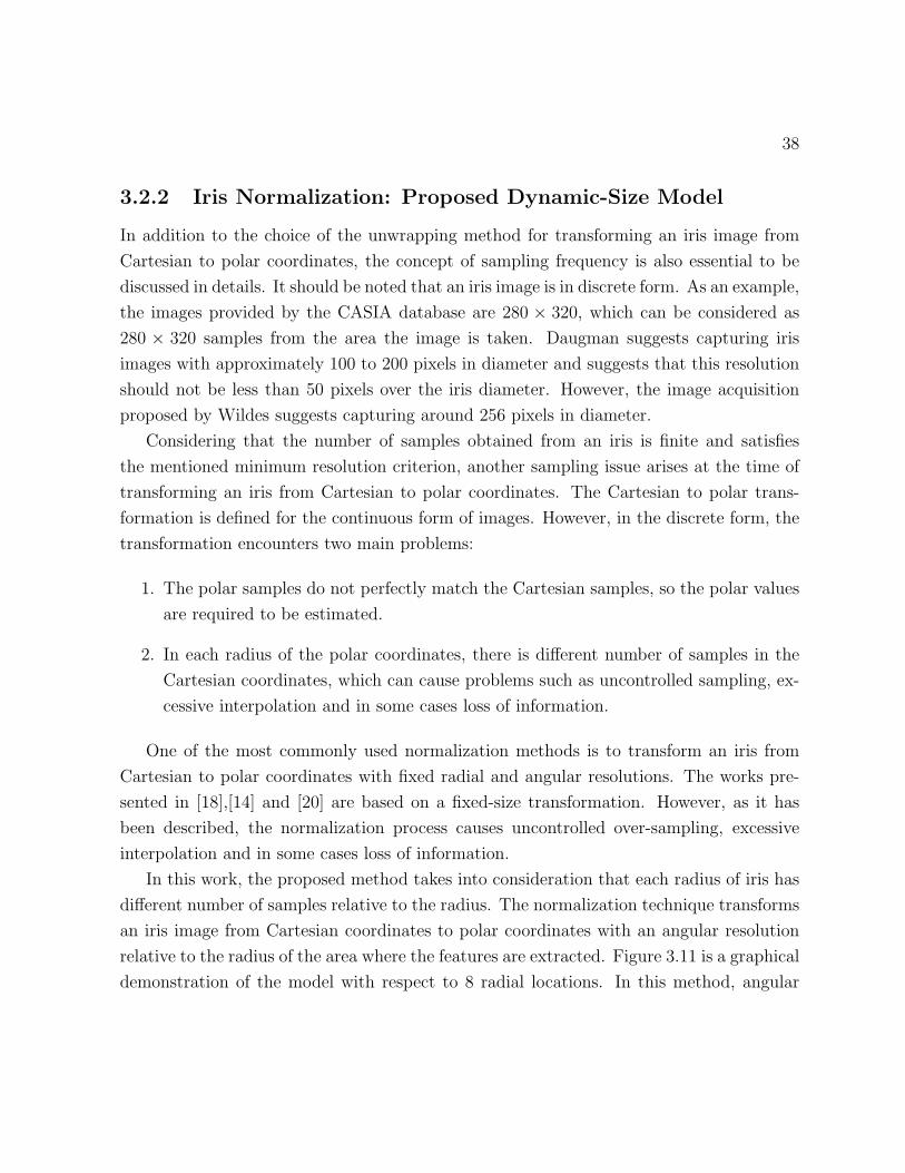
In addition to the choice of the unwrapping method for transforming an iris image from

Cartesian to polar coordinates, the concept of sampling frequency is also essential to be

discussed in details. It should be noted that an iris image is in discrete form. As an example,

the images provided by the CASIA database are 280 × 320, which can be considered as

280 × 320 samples from the area the image is taken. Daugman suggests capturing iris

images with approximately 100 to 200 pixels in diameter and suggests that this resolution

should not be less than 50 pixels over the iris diameter. However, the image acquisition

proposed by Wildes suggests capturing around 256 pixels in diameter.

Considering that the number of samples obtained from an iris is finite and satisfies

the mentioned minimum resolution criterion, another sampling issue arises at the time of

transforming an iris from Cartesian to polar coordinates. The Cartesian to polar trans-

formation is defined for the continuous form of images. However, in the discrete form, the

transformation encounters two main problems:

1. The polar samples do not perfectly match the Cartesian samples, so the polar values

are required to be estimated.

2. In each radius of the polar coordinates, there is different number of samples in the

Cartesian coordinates, which can cause problems such as uncontrolled sampling, ex-

cessive interpolation and in some cases loss of information.

One of the most commonly used normalization methods is to transform an iris from

Cartesian to polar coordinates with fixed radial and angular resolutions. The works pre-

sented in [18],[14] and [20] are based on a fixed-size transformation. However, as it has

been described, the normalization process causes uncontrolled over-sampling, excessive

interpolation and in some cases loss of information.

In this work, the proposed method takes into consideration that each radius of iris has

different number of samples relative to the radius. The normalization technique transforms

an iris image from Cartesian coordinates to polar coordinates with an angular resolution

relative to the radius of the area where the features are extracted. Figure 3.11 is a graphical

demonstration of the model with respect to 8 radial locations. In this method, angular

39

��������

�������

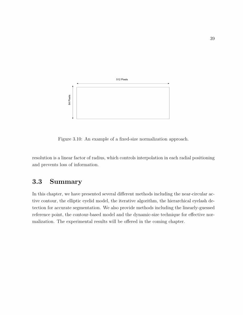
Figure 3.10: An example of a fixed-size normalization approach.

resolution is a linear factor of radius, which controls interpolation in each radial positioning

and prevents loss of information.

3.3 Summary

In this chapter, we have presented several different methods including the near-circular ac-

tive contour, the elliptic eyelid model, the iterative algorithm, the hierarchical eyelash de-

tection for accurate segmentation. We also provide methods including the linearly-guessed

reference point, the contour-based model and the dynamic-size technique for effective nor-

malization. The experimental results will be offered in the coming chapter.

40

K)R2( ×π

�������

���

Figure 3.11: The proposed dynamic-size method. In this method, size of rectangular blocks

are adjusted by perimeter of pupil and limbus boundaries.

Chapter 4

Experimental Results

4.1 Segmentation

4.1.1 Pupil Detection

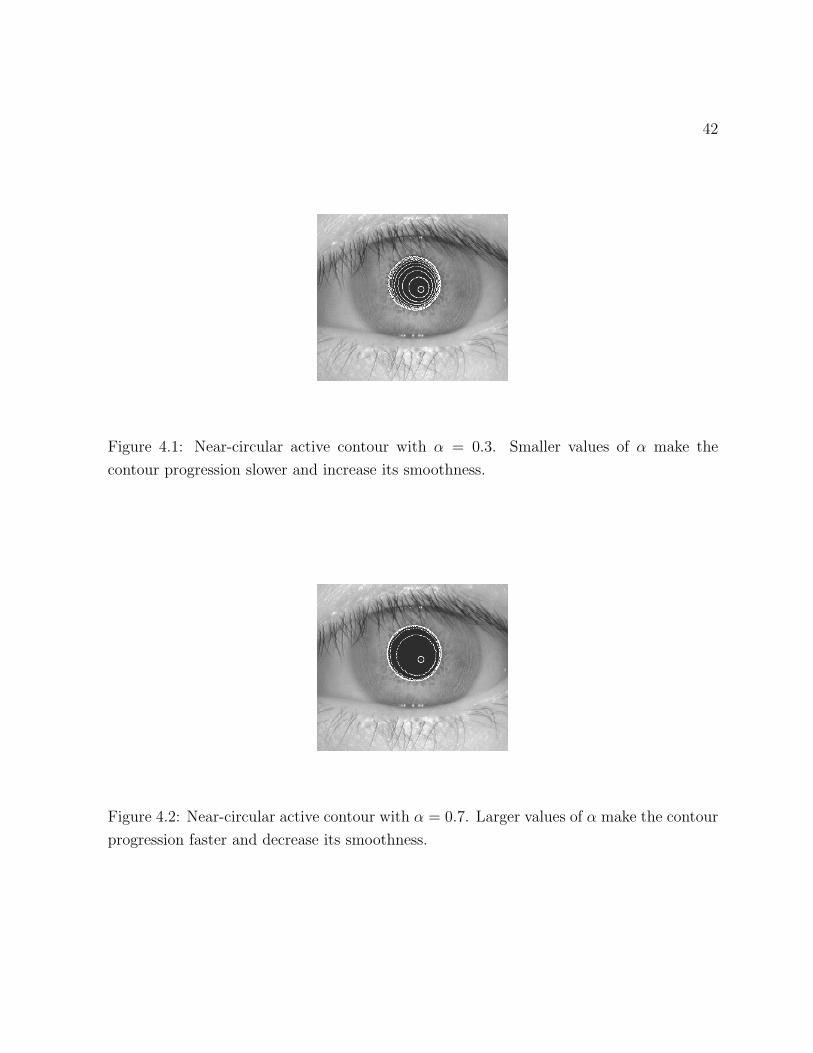
The performance of the proposed active contour with respect to different values of α is

illustrated in figures 4.1 and 4.2. Figure 4.1 shows that smaller values of α generate

smoother contours and the vertices move toward pupil boundary in a slower pace. However,

as it shown in figure 4.2, increasing the value of α, increases the effect of external forces

and makes the contour vertices to move toward the pupil boundary in a faster pace. The

value of α should be smaller than 1 in order to prevent the contour from oscillating around

the pupil boundary due to the definition of the external forces. It should be mentioned

that the initial center of contour is obtained by first thresholding the image to obtain the

dark regions representing pupil and eyelash regions. In the CASIA database, the value of

the threshold is set to 65 in grey level scale. The center of contour is then initialized as

center of mass of the obtained dark regions.

In addition, the accuracy of the external and internal forces highly depends on the po-

sition of the contour center point. The contour center is the reference point for calculating

the internal and external forces in the defined angular range ∆θ = π10

. As the contour

center becomes closer to the pupil center, the internal and external forces are measured

more accurately because of better adjustment of the angular arcs with respect to the pupil

41

42

Figure 4.1: Near-circular active contour with α = 0.3. Smaller values of α make the

contour progression slower and increase its smoothness.

Figure 4.2: Near-circular active contour with α = 0.7. Larger values of α make the contour

progression faster and decrease its smoothness.

43

boundary. The external forces are designed to pull the curve toward the maximum circular

gradient. The definition of the external forces makes the contour vertices to move in a way

that the contour center gradually becomes closer to the actual pupil center. Therefore,

calculation of the internal and external forces becomes more accurate after each iteration.

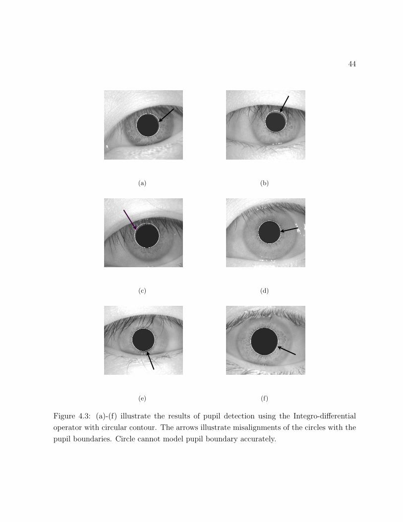
Figure 4.3 illustrates the results of pupil detection using the circular Integro-differential.

It is shown that the actual pupil boundaries would not be properly located when the con-

tours are assumed to be circular. The results of the near-circular active contour are shown

in figure 4.4, where the location of pupil borders of figure 4.3 are detected accurately. In

section 4.2.1, the recognition improvements of the active contour is demonstrated com-

pared to the traditional circular pupil detection. The near-circular active contour has a

100% success rate and is able to accurately detect all the 756 iris images in the CASIA

database.

4.1.2 Eyelid Model

The proposed elliptic eyelid model has shown a great potential in detecting the eyelid

borders. The curve model is defined in the polar coordinates with respect to pupil center.

The search for the eyelid contours is performed by the Integro-differential operator using

the proposed curve model. The search space of the operator is defined based on the polar

representation of equation 3.10 with respect to the pupil center over a range of values for

the Reyeball and θ. The value of Reyeball varies from Rlimbus to 2Rlimbus, where Rlimbus is

the estimated limbus radius in the previous iteration. The value of θ, which defines the

orientation of the eyelid contour, is chosen to vary in the interval [−π8, π

8] to compensate

the possible eye rotations. The fixed choice of angular resolution normalizes the eyelid

contours, where an equal number of samples would be considered over each curve at the

time the Integro-differential operator is applied.

Figure 4.5 illustrates some of the successful eyelid detections. The dark areas in the

images are the iris textures that are covered by the eyelids which are excluded for the

feature extraction and matching process.

This model has been able to accurately detect eyelids of 708 images out of the 756

images in the CASIA database. In addition, different cases of unsuccessful detection are

studied. There are three main cases where the eyelids are not properly detected. Figure 4.6

44

(a) (b)

(c) (d)

(e) (f)

Figure 4.3: (a)-(f) illustrate the results of pupil detection using the Integro-differential

operator with circular contour. The arrows illustrate misalignments of the circles with the

pupil boundaries. Circle cannot model pupil boundary accurately.

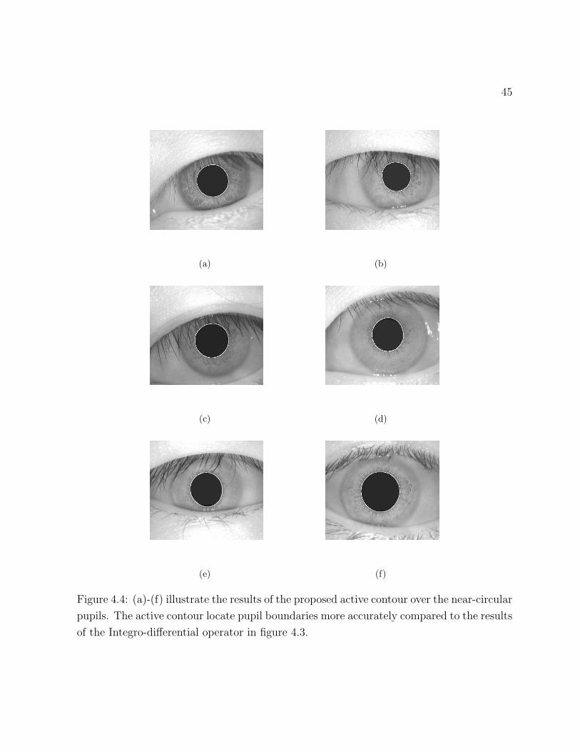
45

(a) (b)

(c) (d)

(e) (f)

Figure 4.4: (a)-(f) illustrate the results of the proposed active contour over the near-circular

pupils. The active contour locate pupil boundaries more accurately compared to the results

of the Integro-differential operator in figure 4.3.

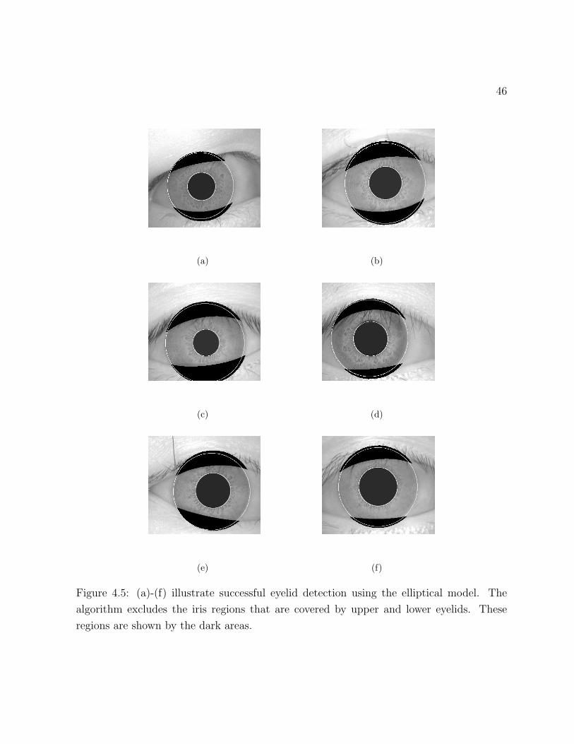
46

(a) (b)

(c) (d)

(e) (f)

Figure 4.5: (a)-(f) illustrate successful eyelid detection using the elliptical model. The

algorithm excludes the iris regions that are covered by upper and lower eyelids. These

regions are shown by the dark areas.

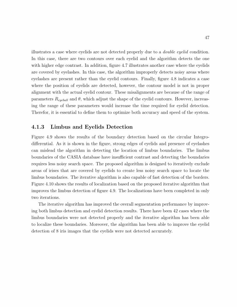
47

illustrates a case where eyelids are not detected properly due to a double eyelid condition.

In this case, there are two contours over each eyelid and the algorithm detects the one

with higher edge contrast. In addition, figure 4.7 illustrates another case where the eyelids

are covered by eyelashes. In this case, the algorithm improperly detects noisy areas where

eyelashes are present rather than the eyelid contours. Finally, figure 4.8 indicates a case

where the position of eyelids are detected, however, the contour model is not in proper

alignment with the actual eyelid contour. These misalignments are because of the range of

parameters Reyeball and θ, which adjust the shape of the eyelid contours. However, increas-

ing the range of these parameters would increase the time required for eyelid detection.

Therefor, it is essential to define them to optimize both accuracy and speed of the system.

4.1.3 Limbus and Eyelids Detection

Figure 4.9 shows the results of the boundary detection based on the circular Integro-

differential. As it is shown in the figure, strong edges of eyelids and presence of eyelashes

can mislead the algorithm in detecting the location of limbus boundaries. The limbus

boundaries of the CASIA database have insufficient contrast and detecting the boundaries

requires less noisy search space. The proposed algorithm is designed to iteratively exclude

areas of irises that are covered by eyelids to create less noisy search space to locate the

limbus boundaries. The iterative algorithm is also capable of fast detection of the borders.

Figure 4.10 shows the results of localization based on the proposed iterative algorithm that

improves the limbus detection of figure 4.9. The localizations have been completed in only

two iterations.

The iterative algorithm has improved the overall segmentation performance by improv-

ing both limbus detection and eyelid detection results. There have been 42 cases where the

limbus boundaries were not detected properly and the iterative algorithm has been able

to localize these boundaries. Moreover, the algorithm has been able to improve the eyelid

detection of 8 iris images that the eyelids were not detected accurately.

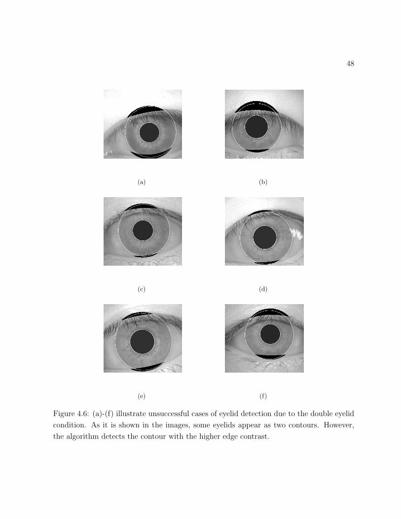
48

(a) (b)

(c) (d)

(e) (f)

Figure 4.6: (a)-(f) illustrate unsuccessful cases of eyelid detection due to the double eyelid

condition. As it is shown in the images, some eyelids appear as two contours. However,

the algorithm detects the contour with the higher edge contrast.

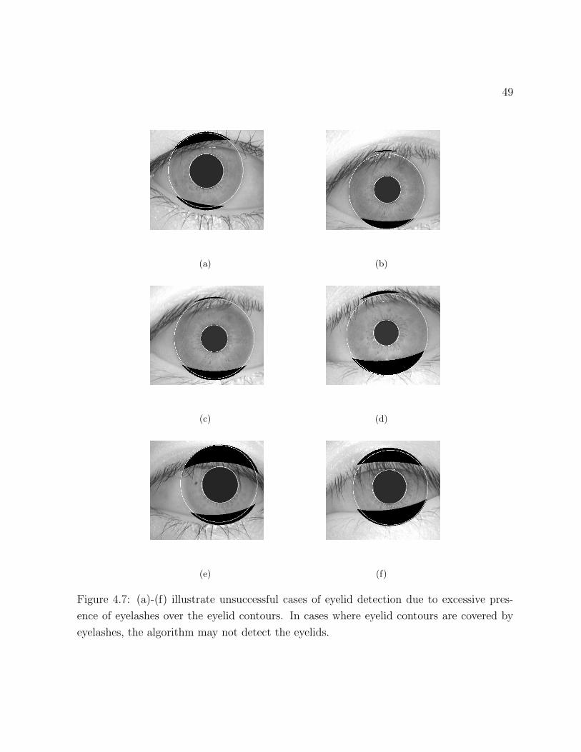
49

(a) (b)

(c) (d)

(e) (f)

Figure 4.7: (a)-(f) illustrate unsuccessful cases of eyelid detection due to excessive pres-

ence of eyelashes over the eyelid contours. In cases where eyelid contours are covered by

eyelashes, the algorithm may not detect the eyelids.

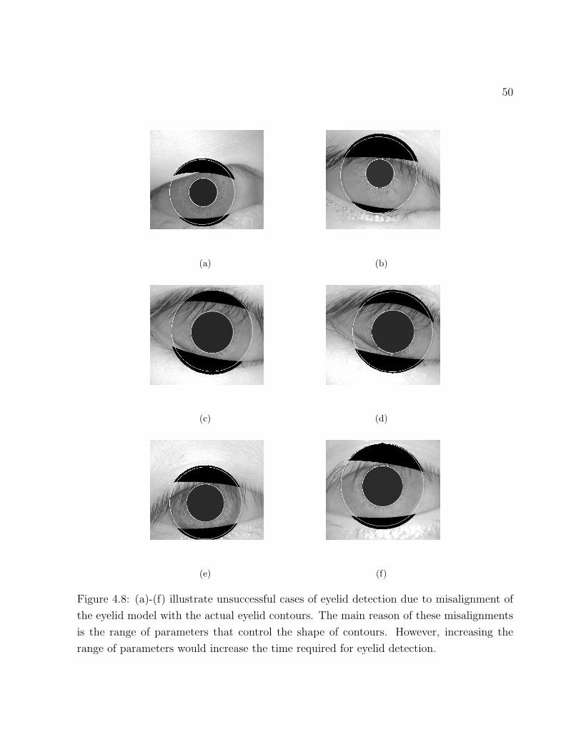
50

(a) (b)

(c) (d)

(e) (f)

Figure 4.8: (a)-(f) illustrate unsuccessful cases of eyelid detection due to misalignment of

the eyelid model with the actual eyelid contours. The main reason of these misalignments

is the range of parameters that control the shape of contours. However, increasing the

range of parameters would increase the time required for eyelid detection.

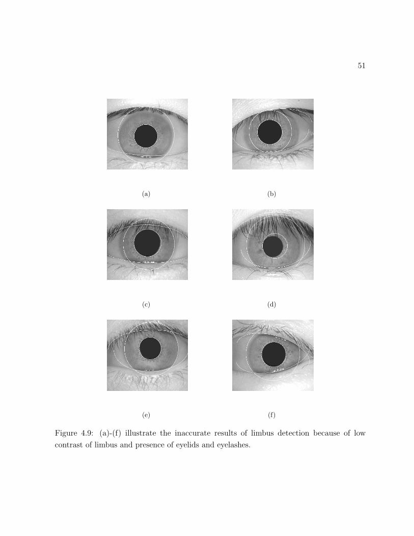
51

(a) (b)

(c) (d)

(e) (f)

Figure 4.9: (a)-(f) illustrate the inaccurate results of limbus detection because of low

contrast of limbus and presence of eyelids and eyelashes.

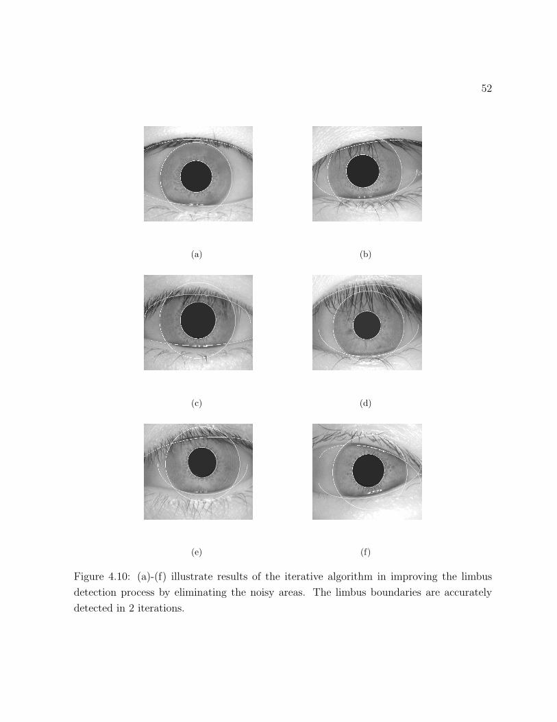
52

(a) (b)

(c) (d)

(e) (f)

Figure 4.10: (a)-(f) illustrate results of the iterative algorithm in improving the limbus

detection process by eliminating the noisy areas. The limbus boundaries are accurately

detected in 2 iterations.

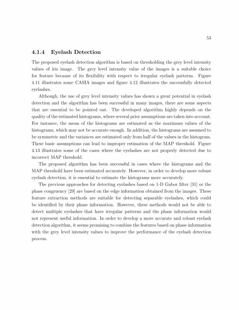
53

4.1.4 Eyelash Detection

The proposed eyelash detection algorithm is based on thresholding the grey level intensity

values of iris image. The grey level intensity value of the images is a suitable choice

for feature because of its flexibility with respect to irregular eyelash patterns. Figure

4.11 illustrates some CASIA images and figure 4.12 illustrates the successfully detected

eyelashes.

Although, the use of grey level intensity values has shown a great potential in eyelash

detection and the algorithm has been successful in many images, there are some aspects

that are essential to be pointed out. The developed algorithm highly depends on the

quality of the estimated histograms, where several prior assumptions are taken into account.

For instance, the mean of the histograms are estimated as the maximum values of the

histograms, which may not be accurate enough. In addition, the histograms are assumed to

be symmetric and the variances are estimated only from half of the values in the histogram.

These basic assumptions can lead to improper estimation of the MAP threshold. Figure

4.13 illustrates some of the cases where the eyelashes are not properly detected due to

incorrect MAP threshold.

The proposed algorithm has been successful in cases where the histograms and the

MAP threshold have been estimated accurately. However, in order to develop more robust

eyelash detection, it is essential to estimate the histograms more accurately.

The previous approaches for detecting eyelashes based on 1-D Gabor filter [31] or the

phase congruency [29] are based on the edge information obtained from the images. These

feature extraction methods are suitable for detecting separable eyelashes, which could

be identified by their phase information. However, these methods would not be able to

detect multiple eyelashes that have irregular patterns and the phase information would

not represent useful information. In order to develop a more accurate and robust eyelash

detection algorithm, it seems promising to combine the features based on phase information

with the grey level intensity values to improve the performance of the eyelash detection

process.

54

(a) (b)

(c) (d)

(e) (f)

Figure 4.11: (a)-(f) illustrate some eye images from CASIA database.

55

(a) (b)

(c) (d)

(e) (f)

Figure 4.12: (a)-(f) illustrate the results of the eyelash detection algorithm. The algorithm

is based on MAP classification combined with a connectivity criterion. The connectivity

criterion assumes that an eyelash pixel is either connected to another eyelash pixel or to

the detected eyelid contours.

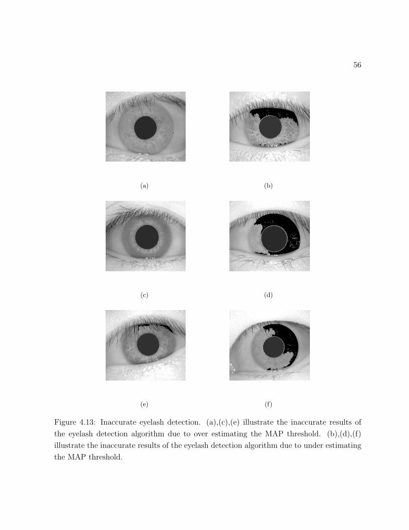
56

(a) (b)

(c) (d)

(e) (f)

Figure 4.13: Inaccurate eyelash detection. (a),(c),(e) illustrate the inaccurate results of

the eyelash detection algorithm due to over estimating the MAP threshold. (b),(d),(f)

illustrate the inaccurate results of the eyelash detection algorithm due to under estimating

the MAP threshold.

57

4.2 Normalization

In the field of iris recognition, performance of most systems are compared to the algo-

rithm proposed by Daugman, which is considered as the state-of-the-art in the field. A

Daugman-like algorithm has been developed to test different methods of segmentation and

normalization to better demonstrate their impact on the system. Because of the differences

in the implementation of the algorithm and the different images used in our experiments

compared to other works, the results are based on demonstrating improvements within

the developed algorithm to present a fair comparison of various techniques. 424 properly

localized iris images are used throughout all the experiments and the Daugman‘s feature

extraction method, 2D Gabor filter, is used to create the iris templates.

In order to illustrate the effect of different normalization methods on performance of

the system, the recognition results are examined. The developed 2D Gabor filter of the

Daugman-like algorithm has been used and the decidability index, d’, of the methods are

compared. The 2D Gabor filter is defined as:

h(Re,Im) = sgn(Re,Im)

∫

ρ

∫

φ

I(ρ, φ)e−jω(θ0−φ)e−(r0−ρ)2/α2

e−(θ0−φ)2/β2

ρdρdφ, (4.1)

where I(ρ, φ) is the raw iris image in the dimensionless polar coordinates. α and β are

the multi-scale 2D wavelet size parameters and ω is the wavelet frequency. (r0, θ0) are the

polar coordinates of each region of iris that the features are computed. The iris templates

of our experiments are obtained by applying the Gabor filter in 8 × 128 = 1024 locations

of the iris textures. The 8× 128 indicates 8 radial locations and 128 angular locations and

the templates are 2048 bits, where 2 bits are extracted from each location of iris due to

the phase demodulation process.

The radial resolution of I(ρ, φ) and the value of α are fixed throughout all the experi-

ments in order to reduce the number of changing parameters. The radial resolution of the

polar images are fixed to 90 pixels, which is chosen based on an initial experiment. In this

experiment, the d’ index of different angular and radial resolutions are obtained over a

smaller iris database. Using these values, two average d’ graphs are obtained by averaging

over the angular and radial resolutions. Figure 4.14 illustrates the average d’ over the

radial resolutions varying from 9 to 180 pixels with respect to angular resolution. Figure

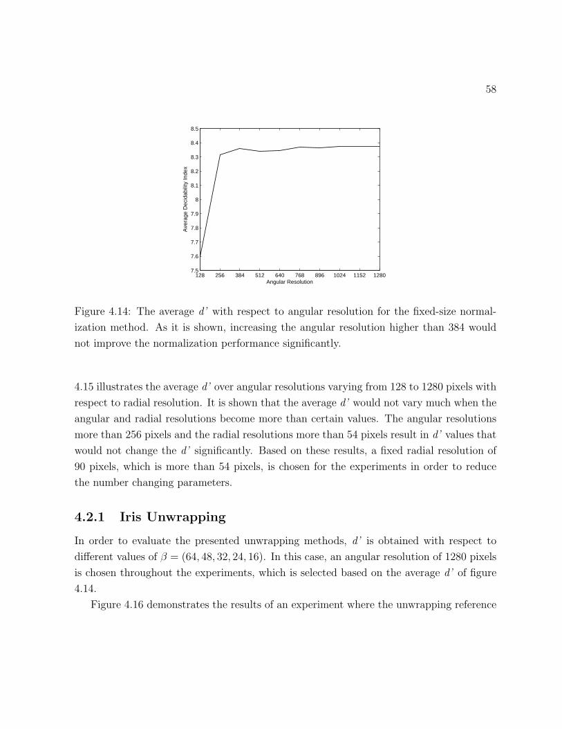
58

128 256 384 512 640 768 896 1024 1152 12807.5

7.6

7.7

7.8

7.9

8

8.1

8.2

8.3

8.4

8.5

Angular Resolution

Ave

rage

Dec

idab

ility

Inde

x

Figure 4.14: The average d’ with respect to angular resolution for the fixed-size normal-

ization method. As it is shown, increasing the angular resolution higher than 384 would

not improve the normalization performance significantly.

4.15 illustrates the average d’ over angular resolutions varying from 128 to 1280 pixels with

respect to radial resolution. It is shown that the average d’ would not vary much when the

angular and radial resolutions become more than certain values. The angular resolutions

more than 256 pixels and the radial resolutions more than 54 pixels result in d’ values that

would not change the d’ significantly. Based on these results, a fixed radial resolution of

90 pixels, which is more than 54 pixels, is chosen for the experiments in order to reduce

the number changing parameters.

4.2.1 Iris Unwrapping

In order to evaluate the presented unwrapping methods, d’ is obtained with respect to

different values of β = (64, 48, 32, 24, 16). In this case, an angular resolution of 1280 pixels

is chosen throughout the experiments, which is selected based on the average d’ of figure

4.14.

Figure 4.16 demonstrates the results of an experiment where the unwrapping reference

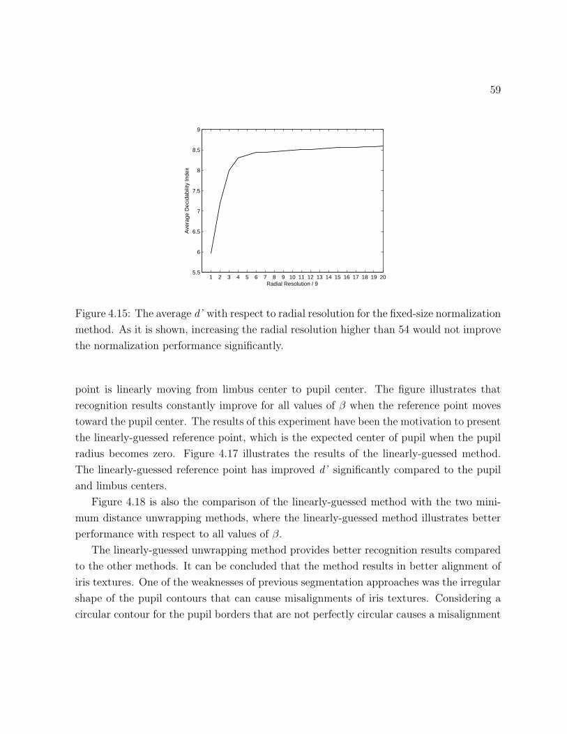
59

1 2 3 4 5 6 7 8 9 10 11 12 13 14 15 16 17 18 19 205.5

6

6.5

7

7.5

8

8.5

9

Radial Resolution / 9

Ave

rage

Dec

idab

ility

Inde

x

Figure 4.15: The average d’ with respect to radial resolution for the fixed-size normalization

method. As it is shown, increasing the radial resolution higher than 54 would not improve

the normalization performance significantly.

point is linearly moving from limbus center to pupil center. The figure illustrates that

recognition results constantly improve for all values of β when the reference point moves

toward the pupil center. The results of this experiment have been the motivation to present

the linearly-guessed reference point, which is the expected center of pupil when the pupil

radius becomes zero. Figure 4.17 illustrates the results of the linearly-guessed method.

The linearly-guessed reference point has improved d’ significantly compared to the pupil

and limbus centers.

Figure 4.18 is also the comparison of the linearly-guessed method with the two mini-

mum distance unwrapping methods, where the linearly-guessed method illustrates better

performance with respect to all values of β.

The linearly-guessed unwrapping method provides better recognition results compared

to the other methods. It can be concluded that the method results in better alignment of

iris textures. One of the weaknesses of previous segmentation approaches was the irregular

shape of the pupil contours that can cause misalignments of iris textures. Considering a

circular contour for the pupil borders that are not perfectly circular causes a misalignment

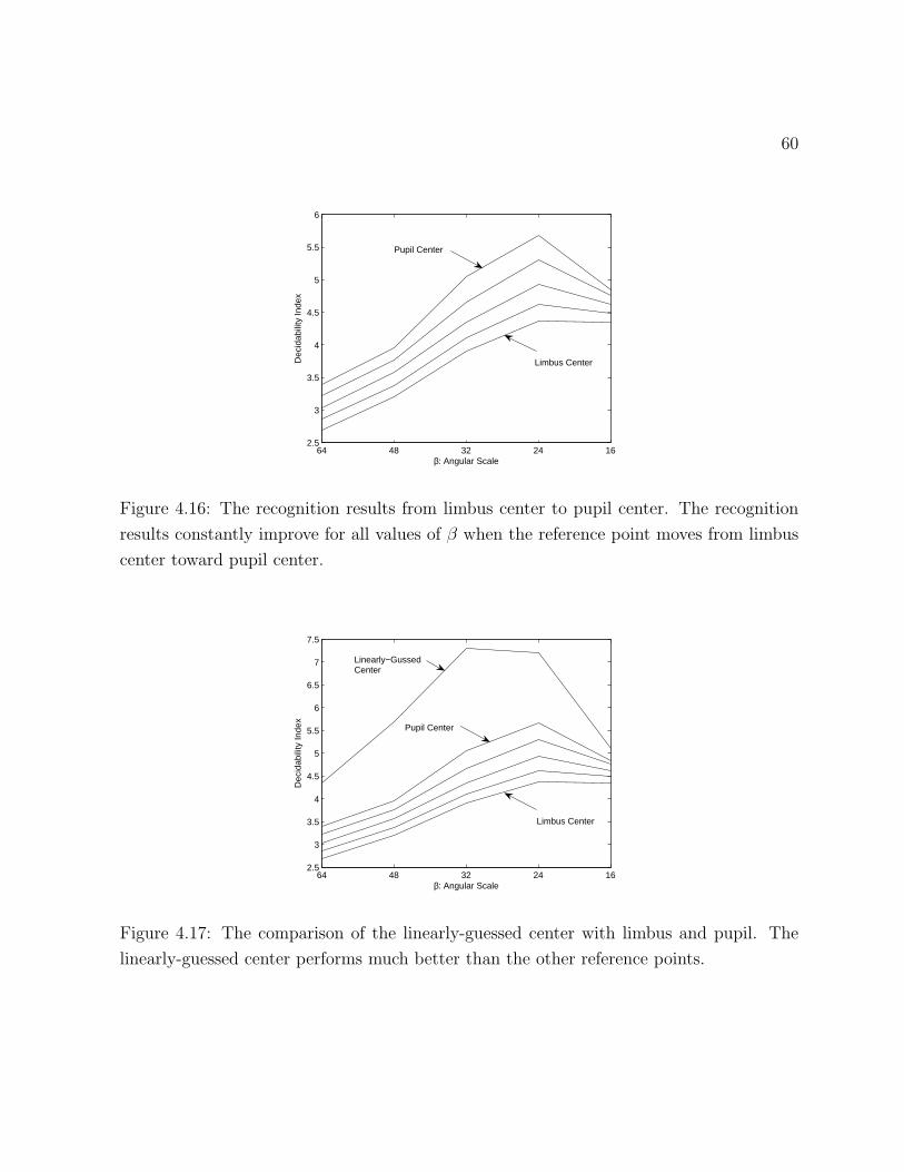
60

64 48 32 24 162.5

3

3.5

4

4.5

5

5.5

6

β: Angular Scale

Dec

idab

ility

Inde

x

Pupil Center

Limbus Center

Figure 4.16: The recognition results from limbus center to pupil center. The recognition

results constantly improve for all values of β when the reference point moves from limbus

center toward pupil center.

64 48 32 24 162.5

3

3.5

4

4.5

5

5.5

6

6.5

7

7.5

β: Angular Scale

Dec

idab

ility

Inde

x

Pupil Center

Limbus Center

Linearly−GussedCenter

Figure 4.17: The comparison of the linearly-guessed center with limbus and pupil. The

linearly-guessed center performs much better than the other reference points.

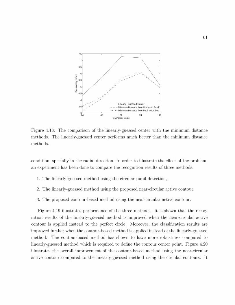
61

64 48 32 24 163

3.5

4

4.5

5

5.5

6

6.5

7

7.5

β: Angular Scale

Dec

idab

ility

Inde

x

Linearly−Guessed CenterMinimum Distance from Limbus to PupilMinimum Distance from Pupil to Limbus

Figure 4.18: The comparison of the linearly-guessed center with the minimum distance

methods. The linearly-guessed center performs much better than the minimum distance

methods.

condition, specially in the radial direction. In order to illustrate the effect of the problem,

an experiment has been done to compare the recognition results of three methods:

1. The linearly-guessed method using the circular pupil detection,

2. The linearly-guessed method using the proposed near-circular active contour,

3. The proposed contour-based method using the near-circular active contour.

Figure 4.19 illustrates performance of the three methods. It is shown that the recog-

nition results of the linearly-guessed method is improved when the near-circular active

contour is applied instead to the perfect circle. Moreover, the classification results are

improved further when the contour-based method is applied instead of the linearly-guessed

method. The contour-based method has shown to have more robustness compared to

linearly-guessed method which is required to define the contour center point. Figure 4.20

illustrates the overall improvement of the contour-based method using the near-circular

active contour compared to the linearly-guessed method using the circular contours. It

62

64 48 32 24 164

4.5

5

5.5

6

6.5

7

7.5

8

β: Angular Scale

Dec

idab

ility

Inde

x

Linearly−Guessed with Perfect CircleLinearly−Guessed with ContourContour−Based with Contour

Figure 4.19: The impact of the active contour and the contour-based unwrapping method.

This figure illustrates that the proposed active contour would improve the the recognition

results compared to the circular pupil detection method. It is also demonstrated that the

proposed contour-based method would further improve the performance compared to the

linearly-guessed method.

should be mentioned that our experiments are designed to depict the improvements of the

system regardless of the choice of parameters such as β. Therefore, the experiments are

designed to test different values of β and illustrate the improvements in each choice of the

parameter. The experiments demonstrate the improvement of the overall performance of

the system with respect to different unwrapping methods.

4.2.2 Iris Normalization

Two different sampling approaches have been introduced: The commonly used fixed-size

sampling and the proposed dynamic sampling. In order to evaluate and compare the

two methods, the recognition results are obtained with respect to different values of β =

(48, 32, 24). It should be reminded that α and the radial resolution are fixed throughout

the experiments. Therefore, in the main formulation of the Gabor filter, equation 4.1, the

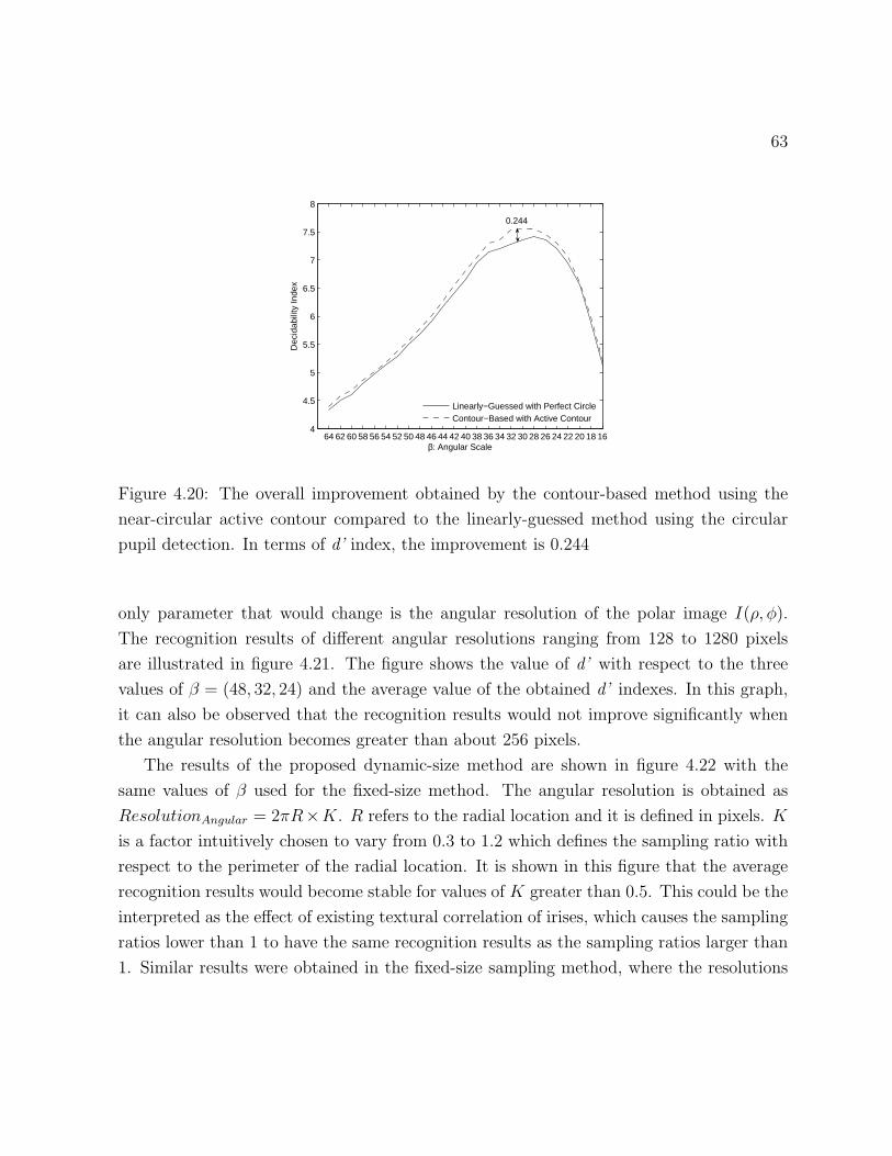
63

64 62 60 58 56 54 52 50 48 46 44 42 40 38 36 34 32 30 28 26 24 22 20 18 164

4.5

5

5.5

6

6.5

7

7.5

8

β: Angular Scale

Dec

idab

ility

Inde

x

Linearly−Guessed with Perfect CircleContour−Based with Active Contour

0.244

Figure 4.20: The overall improvement obtained by the contour-based method using the

near-circular active contour compared to the linearly-guessed method using the circular

pupil detection. In terms of d’ index, the improvement is 0.244

only parameter that would change is the angular resolution of the polar image I(ρ, φ).

The recognition results of different angular resolutions ranging from 128 to 1280 pixels

are illustrated in figure 4.21. The figure shows the value of d’ with respect to the three

values of β = (48, 32, 24) and the average value of the obtained d’ indexes. In this graph,

it can also be observed that the recognition results would not improve significantly when

the angular resolution becomes greater than about 256 pixels.

The results of the proposed dynamic-size method are shown in figure 4.22 with the

same values of β used for the fixed-size method. The angular resolution is obtained as

ResolutionAngular = 2πR×K. R refers to the radial location and it is defined in pixels. K

is a factor intuitively chosen to vary from 0.3 to 1.2 which defines the sampling ratio with

respect to the perimeter of the radial location. It is shown in this figure that the average

recognition results would become stable for values of K greater than 0.5. This could be the

interpreted as the effect of existing textural correlation of irises, which causes the sampling

ratios lower than 1 to have the same recognition results as the sampling ratios larger than

1. Similar results were obtained in the fixed-size sampling method, where the resolutions

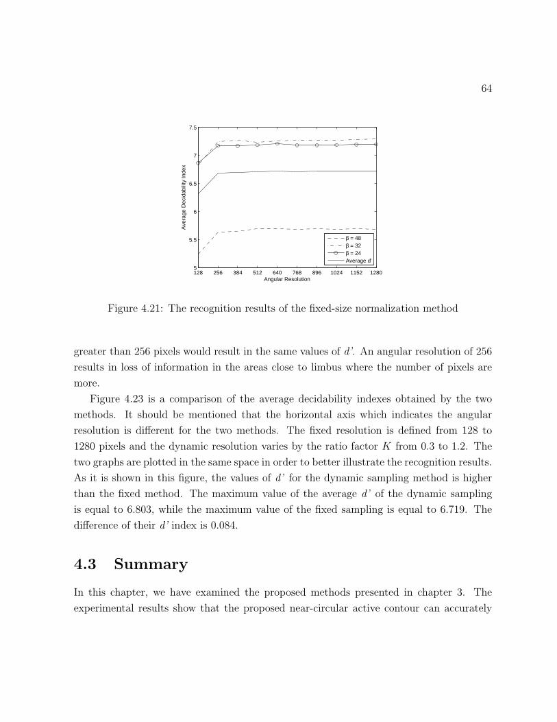
64

128 256 384 512 640 768 896 1024 1152 12805

5.5

6

6.5

7

7.5

Angular Resolution

Ave

rage

Dec

idab

ility

Inde

x

β = 48β = 32β = 24Average d′

Figure 4.21: The recognition results of the fixed-size normalization method

greater than 256 pixels would result in the same values of d’. An angular resolution of 256

results in loss of information in the areas close to limbus where the number of pixels are

more.

Figure 4.23 is a comparison of the average decidability indexes obtained by the two

methods. It should be mentioned that the horizontal axis which indicates the angular

resolution is different for the two methods. The fixed resolution is defined from 128 to

1280 pixels and the dynamic resolution varies by the ratio factor K from 0.3 to 1.2. The

two graphs are plotted in the same space in order to better illustrate the recognition results.

As it is shown in this figure, the values of d’ for the dynamic sampling method is higher

than the fixed method. The maximum value of the average d’ of the dynamic sampling

is equal to 6.803, while the maximum value of the fixed sampling is equal to 6.719. The

difference of their d’ index is 0.084.

4.3 Summary

In this chapter, we have examined the proposed methods presented in chapter 3. The

experimental results show that the proposed near-circular active contour can accurately

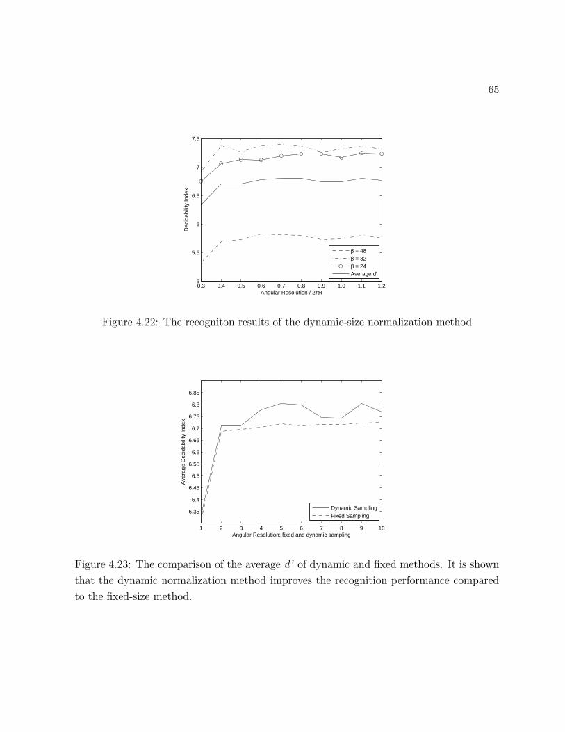
65

0.3 0.4 0.5 0.6 0.7 0.8 0.9 1.0 1.1 1.25

5.5

6

6.5

7

7.5

Angular Resolution / 2πR

Dec

idab

ility

Inde

x

β = 48β = 32β = 24Average d′

Figure 4.22: The recogniton results of the dynamic-size normalization method

1 2 3 4 5 6 7 8 9 10

6.35

6.4

6.45

6.5

6.55

6.6

6.65

6.7

6.75

6.8

6.85

Angular Resolution: fixed and dynamic sampling

Ave

rage

Dec

idab

ility

Inde

x

Dynamic SamplingFixed Sampling

Figure 4.23: The comparison of the average d’ of dynamic and fixed methods. It is shown

that the dynamic normalization method improves the recognition performance compared

to the fixed-size method.

66

detect all the pupil boundaries in the CASIA database. They also indicate that com-

bining the near-circular active contour and the contour-based normalization method can

effectively enhance the performance. In terms of d’ index, the improvement is 0.244. Com-

paring several normalization methods, our experiments pinpoint that the contour-based

method provides the best performance. We also compare the dynamic-size and fixed-size

normalization approaches. This comparison shows that the dynamic method is slightly

more accurate than the fixed-size method. The difference of their d’ index is 0.084.

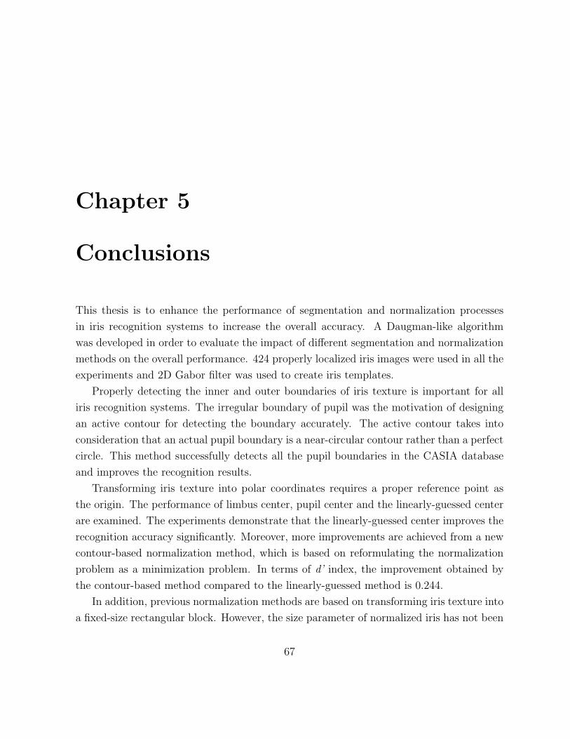
Chapter 5

Conclusions

This thesis is to enhance the performance of segmentation and normalization processes

in iris recognition systems to increase the overall accuracy. A Daugman-like algorithm

was developed in order to evaluate the impact of different segmentation and normalization

methods on the overall performance. 424 properly localized iris images were used in all the

experiments and 2D Gabor filter was used to create iris templates.

Properly detecting the inner and outer boundaries of iris texture is important for all

iris recognition systems. The irregular boundary of pupil was the motivation of designing

an active contour for detecting the boundary accurately. The active contour takes into

consideration that an actual pupil boundary is a near-circular contour rather than a perfect

circle. This method successfully detects all the pupil boundaries in the CASIA database

and improves the recognition results.

Transforming iris texture into polar coordinates requires a proper reference point as

the origin. The performance of limbus center, pupil center and the linearly-guessed center

are examined. The experiments demonstrate that the linearly-guessed center improves the

recognition accuracy significantly. Moreover, more improvements are achieved from a new

contour-based normalization method, which is based on reformulating the normalization

problem as a minimization problem. In terms of d’ index, the improvement obtained by

the contour-based method compared to the linearly-guessed method is 0.244.

In addition, previous normalization methods are based on transforming iris texture into

a fixed-size rectangular block. However, the size parameter of normalized iris has not been

67

68

investigated in details. According to our experiments, the optimal parameter for fixed-

size rectangular shape is 54 × 384. Further increasing the size of the rectangle would not

improve the normalization performance significantly. In addition to evaluating the fixed-

size approach, a dynamic normalization method is proposed. Experimental results show

that the dynamic method can improve the recognition performance. In terms of d’ index,

the improvement is 0.084.

Bibliography

[1] F. H. Adler, “hysiology of the Eye.” St. Louis, MO: Mosby, 1965.

[2] A. Bertillon, “a couleur de liris.” Rev. Sci., vol. 36, no. 3, pp. 6573, 1885.

[3] L. Flom and A. Safir, “ris recognition system.” U.S. Patent 4 641 349, 1987.

[4] Obaidat, M.S., Sadoun, B.: “Verification of computer users using keystroke dynamics.”

IEEE Transactions on Systems, Man and Cybernetics 27 (1997) 261269.

[5] C. Shannon and W. Weaver, “he Mathematical Theory of Communication.” U. Illinois

Press, Urbana, Ill., 1949.

[6] J.G Daugman. “ris recognition.” American Scientist, July-Aug. 2001.

[7] J.G Daugman, “High Confidence Visual Recognition of Persons by a Test of Statistical

Independence.” IEEE Transactions On Pattern Analysis and Machine Intelligence, Vol.

15, No.11, pp.1148-1161,Nov. 1993.

[8] J.G Daugman. “How iris recognition works.” Proceedings of 2002 International Con-

ference on Image Processing, Vol. 1, 2002.

[9] J.G Daugman, “The importance of being random: Statistical principles of iris recogni-

tion.” in Pattern Recognition, Vol. 36, No. 2, pp. 279–291, 2003.

[10] J.G Daugman, “Demodulation by Complex-Valued Wavelets for Stochastic Pattern

Recognition.” Int’l J. Wavelets, Multiresolution and Information Processing, vol. 1, no.

1, pp. 1-17, 2003.

69

70

[11] R. Wildes, J.C. Asmuth, G.L. Green, S.C. Hsu, R.J. Kolczynski, J.R. Matey and

S.E. McBride, “A system for automated iris recognition.” In Proceedings of the IEEE

Workshop on Applications of Computer Vision, pp. 121-128, 1994.

[12] R. Wildes J. Asmuth G. Green S. Hsu R. Kolczynski J. Matey and S. McBride, “A

Machine-Vision System for Iris Recognition.” Machine Vision and Applications, vol. 9,

pp. 1-8, 1996.

[13] R. Wildes, “Iris Recognition: an Emerging Biometric Technology.” Proceeding of the

IEEE, Vol. 85, No. 9, 1997.

[14] W.W. Boles, “A wavelet transform based technique for the recognition of the hu-

man iris.” In Proceedings of the International Symposium on Signal Processing and its

Application, ISSPA, Gold Coast, Australia, pp. 25-30, August, 1996.

[15] W.W. Boles and B. Boashash, “A human identification technique using images of the

iris and wavelet transform.” IEEE Transactions on Signal Processing, vol. 46, no. 4,

pp. 1185-1188, 1998.

[16] C. Tisse L. Martin L. Torres and M. Robert, “Person Identification Technique Using

Human Iris Recognition.” Proc. Vision Interface, pp. 294-299, 2002.

[17] Y. Zhu, T. Tan and Y. Wang “Biometric personal identification based on iris pattern.”

Proceeding of. 15th International Conference on Pattern Recognition, vol. 2, pp. 801-

804, 2000.

[18] S. Lim K. Lee O. Byeon and T. Kim, “Efficient Iris Recognition through Improvement

of Feature Vector and Classifier.” ETRI J., vol. 23, no. 2, pp. 61-70, 2001.

[19] S. Noh, K. Pae, C. Lee, J. Kim. “Multiresolution independent component analysis for

iris identification.” The 2002 International Technical Conference on Circuits/Systems,

Computers and Communications, Phuket, Thailand, 2002.

[20] L. Ma, Y. Wang, T. Tan. “Iris recognition using circular symmetric filters.” National

Laboratory of Pattern Recognition, Institute of Automation, Chinese Academy of Sci-

ences, 2002.

71

[21] C. Seal, M. Gifford and D. McCartney, “Iris recognition for user validation.” British

Telecommunications Engineering Journal, vol. 16, pp. 113-117, July 1997.

[22] M. Negin, T.A. Jr, M. Salganicoff, T.A. Camus, U.M. von Seelen, P.L. Venetianer and

G.G. Zhang, “An iris biometric system for public and personal use.” Computer, vol.

33, no. 2 , pp. 70-75, 2000.

[23] G.O. Williams, “Iris recognition.” IEEE Aerospace and Electronics Systems Magazine,

vol.12, no. 4, pp. 23-29, April 1997.

[24] K. Hanna, R. Mandelbaum, L. Wixson, D. Mishra, and V. Paragana, “A system for

nonintrusive human iris acquisition.” In Proc. Int. Association for Pattern Recognition

Workshop on Machine Vision Applications, Tokyo, Japan, 1996, pp. 200203.

[25] W. Ketchantang, S. Derrode, S. Bourennane, L. Martin, “ Video Pupil Tracking for

Iris Based Identification.” In proceeding of 7th International Conference on Advanced

Concepts for Intelligent Vision Systems, ACIVS 2005, Antwerp, Belgium, September

20-23, 2005.

[26] Kang Ryoung Park, Jaihie Kim: “A real-time focusing algorithm for iris recognition

camera.” IEEE Transactions on Systems, Man, and Cybernetics, Part C 35(3): 441-

444 (2005).

[27] Bressloff, P.C., Wood, C.V. and Howarth, P.A. (1996). “Nonlinear shunting model of

the Pupil Light Reflex.” Proc. Royal Soc. B, vol. 263, pp. 953-960.

[28] X. Xie, R. Sudhakar, and H. Zhuang, “Real-time eye feature tracking from a video

image sequence using kalman filter.” IEEE Transactions on Systems, Man and Cyber-

netics, vol. 25, no. 12, pp. 1568-1577, 1995.

[29] J. Huang, Y. Wang, T. Tan, Jiali Cui, “A new iris segmentation method for recog-

nition.” In Proceedings of the 17th International Conference on Pattern Recognition,

ICPR, Volume: 3, pp. 554- 557 Vol.3 2004.

72

[30] W. Kong, D. Zhang. “Accurate iris segmentation based on novel reflection and eyelash

detection model.” Proceedings of 2001 International Symposium on Intelligent Multi-

media, Video and Speech Processing, Hong Kong, 2001.

[31] W. K. Kong and D. Zhang, “Eyelash detection model for accurate iris segmentation.”

in Proceeding of ISCA 16th International Conference on Computers and their Applica-

tions, March 28-30,2001, pp. 204-207, Seattle, Washington, USA.

[32] B. J. Joung, J. O. Kim, C. H. Chung, Key Seo Lee, Wha Young Yim, Sang Hyo

Lee, “ On Improvement for Normalizing Iris Region for a Ubiquitous Computing.” In

Proceedings of International Conference on Computational Science and Its Applications

ICCSA 2005, Singapore, May 9-12, 2005.

[33] X. Yuan, P. Shi, “A Non-linear Normalization Model for Iris Recognition.” In Pro-

ceedings of International Wokshop on Biometric Recognition Systems on Advances in

Biometric Person Authentication, IWBRS 2005, Beijing, China, October 22-23, 2005.

[34] Harry J. Wyatt: “A Minimum-wear-and-tear Meshwork for the Iris.” In: Vision Re-

search. 40 (2000) 2167-2176

[35] N. Ritter, “Location of the Pupil-Iris Border in Slit-Lamp Images of the Cornea.”

Proceedings of the international Conference on Image Analysis and Processing, 1999.

[36] N. J. Ritter and J. R. Cooper, “Locating the iris: A first step to registration and

identification.” in Proc. 9th IASTED International Conference on Signal and Image

Processing, pp. 507-512, IASTED, Aug. 2003.

[37] M. Kass, A. Witkin, D. Terzopoulos. Snakes: “Active Contour Models.” International

Journal of Computer Vision, 1987.

[38] S. Lobregt and M. A. Viergever, “A Discrete dynamic contour model.” IEEE Trans-

actions on Medival Imaging, 14(1), 1995, 12-24.

[39] N. Wiener, “Times Series.” Cambridge, MA: M.I.T. Press, 1949.

[40] J.P.Havlicek, J.W.Havlicek and A.C.bovik, “the analytic image.” IEEE Journal, 1997.

73

[41] J. R. Bergen, P. Anandan, K. Hanna, and R. Hingorani, “Hierarchical model-based

motion estimation.” in Proc. Euro. Conf. Computer Vision, Santa Margherita Ligure,

Italy, 1991, pp. 510.

[42] Chinese Academy of Sciences Institute of Automation. Database of 756 Greyscale

Eye Images. page http://www.sinobiometrics.com.

[43] International Biometrics Group page http://www.biometricgroup.com/.

[44] UK Passport Service page http://www.passport.gov.uk/index.asp.

[45] US Department of Homeland Security page http://www.dhs.gov/dhspublic/.