A Study of Instruction Level Parallelism in Contemporary ... · parallelism can be quantified,...

A Study of Instruction Level Parallelism in Contemporary

Computer Applications

by

Jyotsna Sabarinathan, B.Tech.

Report

Presented to the Faculty of the Graduate School

of The University of Texas at Austin

in Partial Fulfillment

of the Requirements

for the Degree of

Master of Science in Engineering

The University of Texas at Austin

December 1999



APPROVED BY

SUPERVISING COMITEE:

1

Dedication

To my parents and to Prakash,

for their love, support and encouragement

2

Acknowledgments

I would like to thank Dr. Lizy John for her valuable guidance and advice during

the course of this work. I would like to express my gratitude to Dr. Gustavo de

Veciana for agreeing to be the reader for this report. I also want to thank all the

members of the Laboratory for Computer Architecture, particularly Juan Rubio,

for their invaluable help and encouragement. Finally, I would like to thank my

parents and Prakash, for their never failing love and support.

December 3rd, 1999.

3



by

Jyotsna Sabarinathan, M.S.E.

The University of Texas at Austin, 1999

SUPERVISOR: Lizy Kurian John

One of the most important program properties that is regularly exploited in

modern microprocessors is the available instruction level parallelism. This study

examines the limits to the inherent instruction level parallelism in modern

computer applications in several programming languages and application arenas.

We analyze two different metrics in terms of which the available program

parallelism can be quantified, identify their merits and shortcomings and also

perform a comparative study of the parallelism that can be exploited in a few

representative C, C++, Java, DSP and media benchmarks using these metrics.

This work is focused on logical limits rather than implementation issues and

towards this end, we assume an ideal machine with infinite machine level

parallelism (MLP. The available parallelism ranges from 11 to 21000 in the

various benchmarks that we examined, with harmonic means of 125.07 for the C

benchmarks, 179.27 for the C++ benchmarks, 18.76 for the Java programs and

4

239.7 for the DSP benchmarks. Despite the fact that quantitative analysis

methods are expensive with respect to both time and resources, such studies are

going to be essential in understanding the dynamics of program execution on

future architectures, especially when we consider the increasing complexity of

modern day computer systems.

5

Table of Contents

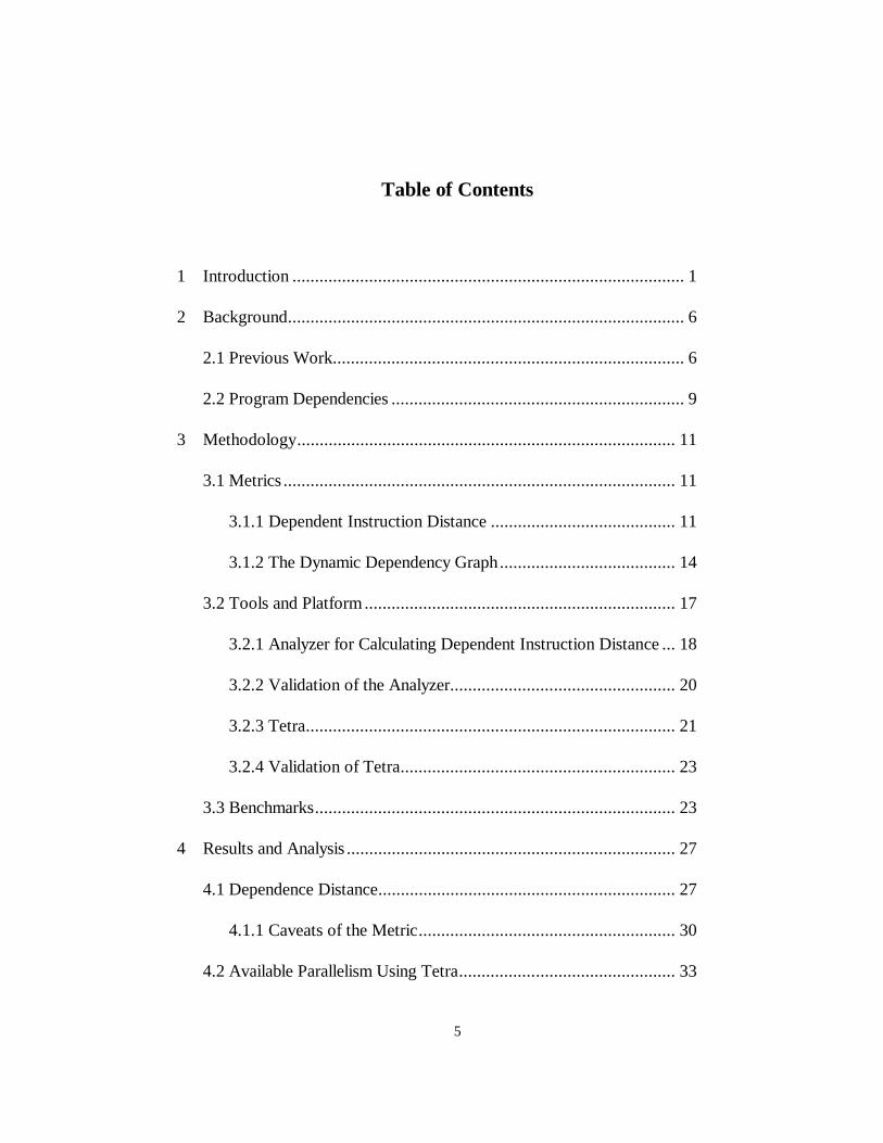
1 Introduction ....................................................................................... 1

2 Background........................................................................................ 6

2.1 Previous Work.............................................................................. 6

2.2 Program Dependencies ................................................................. 9

3 Methodology.................................................................................... 11

3.1 Metrics ....................................................................................... 11

3.1.1 Dependent Instruction Distance ......................................... 11

3.1.2 The Dynamic Dependency Graph....................................... 14

3.2 Tools and Platform..................................................................... 17

3.2.1 Analyzer for Calculating Dependent Instruction Distance ... 18

3.2.2 Validation of the Analyzer.................................................. 20

3.2.3 Tetra.................................................................................. 21

3.2.4 Validation of Tetra............................................................. 23

3.3 Benchmarks................................................................................ 23

4 Results and Analysis ......................................................................... 27

4.1 Dependence Distance.................................................................. 27

4.1.1 Caveats of the Metric......................................................... 30

4.2 Available Parallelism Using Tetra................................................ 33

6

5 Conclusion ....................................................................................... 48

Appendix.......................................................................................... 51

References........................................................................................ 62

Vita ............................................................................................. 65

7

1. Introduction

Understanding the characteristics of workloads is extremely important in the

design of efficient computer architectures. Accurate characterization of workload

behavior leads to the design of improved architectures. The characterization of

applications allows us to tune processor microarchitecture, memory hierarchy

and system architecture to suit particular features in programs. Workload

characterization also has a significant impact on performance evaluation [11].

Understanding the nature of the workload and its intrinsic features can help to

interpret performance measurements and simulation results. Identifying and

characterizing the intrinsic properties of an application in terms of its instruction

level parallelism, control flow behavior, locality, etc. can eventually lead to a

program behavior model, which can be used in conjunction with a processor

model to perform analytical performance modeling of computer systems.

A quantitative analysis of program behavior is thus essential to the computer

architecture design process. Since real workloads differ from each other and each

of them exhibits several interesting intrinsic properties, a study which attempts to

classify programs in terms of system independent parameters can generate results

which can help:

1. In designing system components so as to maximally utilize the unique

characteristics of the workload which typically runs on it. For instance, a

8

study of how much instruction level parallelism actually exists in typical

programs is of particular interest in the context of the continuing trend in

processor architecture to boost the performance of a single processor by

overlapping the execution of more and more operations, using fine-grain

parallel processing models such as VLIW, superscalar, etc.

2. In re-designing programs such that they provide better performance on

existing systems. A study such as the one mentioned above which attempts

to measure the available parallelism in a program can also indicate whether

the performance bottleneck is insufficient parallelism in the instruction

stream. This can lead to an effort to re-design the program with a view to

reducing inter-instruction dependencies, for example, by the use of

appropriate compiler optimizations.

This study attempts to examine the limits to instruction level parallelism that

can be found in some modern representative workloads. We examine a couple of

different metrics in terms of which the available program parallelism can be

quantified, identify their merits and shortcomings and also perform a comparative

study of the parallelism that can be exploited in a few representative C, C++,

Java, DSP and media benchmarks in terms of these metrics.

The amount of instruction level parallelism that is typically available in user

programs has always been a highly debated issue. There are researchers who

9

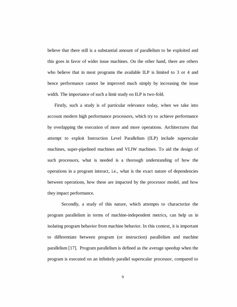
believe that there still is a substantial amount of parallelism to be exploited and

this goes in favor of wider issue machines. On the other hand, there are others

who believe that in most programs the available ILP is limited to 3 or 4 and

hence performance cannot be improved much simply by increasing the issue

width. The importance of such a limit study on ILP is two-fold.

Firstly, such a study is of particular relevance today, when we take into

account modern high performance processors, which try to achieve performance

by overlapping the execution of more and more operations. Architectures that

attempt to exploit Instruction Level Parallelism (ILP) include superscalar

machines, super-pipelined machines and VLIW machines. To aid the design of

such processors, what is needed is a thorough understanding of how the

operations in a program interact, i.e., what is the exact nature of dependencies

between operations, how these are impacted by the processor model, and how

they impact performance.

Secondly, a study of this nature, which attempts to characterize the

program parallelism in terms of machine-independent metrics, can help us in

isolating program behavior from machine behavior. In this context, it is important

to differentiate between program (or instruction) parallelism and machine

parallelism [17]. Program parallelism is defined as the average speedup when the

program is executed on an infinitely parallel superscalar processor, compared to

10

execution on a single-issue processor. Machine parallelism is defined as the

product of the average degree of superpipelining and the degree of parallel issue.

This is effectively the number of instructions “in flight” in the processor. The

overall processor performance can be viewed as the result of the interaction

between program parallelism and machine parallelism in the sense that one is

limited by the other. If the machine parallelism is low relative to program

parallelism, overall performance is limited by the machine parallelism. If, on the

other hand, the machine parallelism is high, program parallelism will be the

limiting factor. Hence, another objective of this study is to extract program

parallelism and use it as one of the parameters to model program behavior. Such

a separation of machine and program parameters can also greatly simplify the

performance evaluation process, especially when we take into account the

increasing complexity of both the computer system being evaluated and the

application used for benchmarking.

The remainder of this report discusses the previous work done in this area,

our methodology of evaluation including tools, metrics and benchmarks used for

the characterization of instruction level parallelism, the results obtained and

finally, analysis and conclusions.

12

2. Background

2.1 Previous Work

There has been a good amount of research directed towards measuring

the exploitable parallelism of an instruction stream. Early studies by Tjaden and

Flynn showed that 2-3 instructions per clock (IPC) were possible [9]. However,

these studies did not consider the possibilities of looking past a branch and were

therefore bound by basic block sizes, which are typically four to eight

instructions. The recognition of the importance of branch prediction as enabling

parallelism lead to a significant effort in branch prediction that continues today

[15]. It is now possible to achieve prediction rates that are correct more than

95% of the time. The possibility of high prediction rates also prompted limit

studies that considered speculative execution scenarios that extended beyond

basic block boundaries.

Many of the earlier limit studies [6,7] also removed WAR and WAW

dependencies in the case of registers by modeling renaming. The use of register

renaming hardware in current processors has given added relevance to these

studies. Work reported by Wall [5] showed that there was a potential for IPC

greater than 60 if perfect prediction was assumed. To achieve this limit, it was

also necessary to assume that caches were perfect, that data dependence analysis

13

could be done essentially instantaneously and that register renaming was

supported.

Austin and Sohi [3] have studied the parallelism in the SPEC 92

benchmarks using the dynamic execution graph technique. Memory renaming

was also considered in this limit study. The study concluded that exposing a

useful amount of parallelism requires renaming of both registers and memory,

though renaming registers alone exposes much of the parallelism. Also, fairly

large windows of dynamic instructions are required to expose this parallelism

from a sequential instruction stream.

More recently, Postiff et.al [4] examined the limits to instruction level

parallelism in the SPEC95 applications. Unlike earlier studies, this study also

removed non-essential true dependencies that occur as a result of the compiler

employing a stack for subroutine linkage. This study showed that a marked

increase in exploitable parallelism can be seen by successive addition of register

renaming, memory renaming, and removal of the compiler-induced dependency

on the stack pointer. The study also concluded that with a limited instruction

window, the IPC of most applications is limited to a value approximately equal to

the register renaming only model.

These limit studies gave an optimistic picture. Other studies that

considered the complexities of the hardware needed to detect data dependencies

14

between instructions, the complexities of fetching non-contiguous instructions

from memory, and gathering multiple data items from memory in single cycles,

arrived at much more pessimistic results that suggested 2-3 as a limit for IPC [7].

Nevertheless, the limit studies showed that the limitations were one of physical

implementation, not logical implementations, and thus provided a realistic goal

for implementers.

This study is a comparative analysis of the limits of instruction level

parallelism demonstrated by a few modern benchmark suites. Instead of confining

the study to the SPEC95 applications, current applications such as C++

programs, Java programs and a set of DSP and media benchmarks have also been

examined. This is significant in today’s scenario, as these applications and

programming paradigms are gaining widespread popularity and acceptance. This

work is focused on logical limits rather than implementation issues and towards

this end, we assume an ideal machine with infinite machine level parallelism

(MLP). For purposes of comparison, we also studied the effect of limiting the

MLP to more feasible values such as 32, 64 and 128.

2.2 Types of Program Dependencies

Program dependencies present a major hurdle to the amount of instruction

level parallelism that can be exploited from a program because they serialize the

execution of instructions. Some dependencies are inherent to the execution of

15

the program and cannot be removed, others can be removed, but usually not

without costs in storage and possibly execution speed. The data dependencies

that are typically present in a program can be classified into the following

categories [3]:

(a) True Data Dependencies

Two operations share a true data dependency if one operation creates a value

that is used by the other (also called a Read-After-Write or RAW dependency).

The dependency forces an order upon operations such that source values are

created before they are used in subsequent operations.

(b) Storage Dependencies

Dependencies can also exist because of a limited amount of storage. Such

storage dependencies require that a computation be delayed until the storage

location for the result is no longer required by previous computations. Storage

dependencies are often further classified and referred to as Write-After-Read

(WAR) and Write-After-Write (WAW) dependencies. Since many different data

values can reside in a single storage location over the lifetime of a program,

synchronization is required to ensure that a computation is accessing the correct

value for that storage location. Violation of a storage dependency would result

in the access of an uninitialized storage location, or another data value stored in

16

the same storage location. Storage dependencies can always be removed by

assigning a new storage location to each value created. This is called renaming.

(c) Control Dependencies

A control dependency is introduced when it is not known which instruction

will be executed next until some previous instruction has completed. Such

dependencies arise because of conditional branch instructions that choose

between several paths of execution based upon the outcome of certain tests.

(d) Resource Dependencies

Resource dependencies (also called structural hazards) occur when

operations must delay because some required physical resource has become

exhausted. Examples of limiting resources in a processor include functional

units, window slots, and physical registers (when renaming is supported).

17

3. Methodology

In this section, we describe the metrics that we used to characterize the

ILP of a program, the tools that were used for the study and the different

categories of benchmarks that were studied.

3.1 Metrics

We attempted to quantitatively characterize the ILP of a given program

as a function of the inherent data dependencies or data flow constraints present in

the program. In this study, we first examined the dependent instruction distance

[2] as a metric to capture program parallelism. However, our results indicated

that this metric is not truly representative, especially in the context of modern,

out-of-order processors. This led us to use the dynamic dependency graph

technique as a means to obtain the available parallelism in terms of the average

number of instructions that can be scheduled per cycle.

3.1.1 Dependent Instruction Distance

Noonberg and Shen [2] used dependent instruction distance as one of the

parameters to model program parallelism. In their approach, each program trace

is scanned once to generate a set of program parallelism parameters, which can

be used across an entire family of machine models. The program parallelism

parameters and the machine model were combined to form a Markov chain,

which statistically models superscalar processor performance.

18

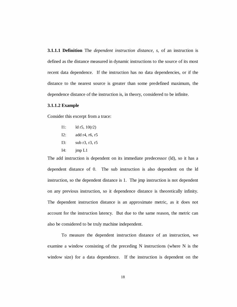
3.1.1.1 Definition The dependent instruction distance, s, of an instruction is

defined as the distance measured in dynamic instructions to the source of its most

recent data dependence. If the instruction has no data dependencies, or if the

distance to the nearest source is greater than some predefined maximum, the

dependence distance of the instruction is, in theory, considered to be infinite.

3.1.1.2 Example

Consider this excerpt from a trace:

I1: ld r5, 10(r2)

I2: add r4, r6, r5

I3: sub r3, r3, r5

I4: jmp L1

The add instruction is dependent on its immediate predecessor (ld), so it has a

dependent distance of 0. The sub instruction is also dependent on the ld

instruction, so the dependent distance is 1. The jmp instruction is not dependent

on any previous instruction, so it dependence distance is theoretically infinity.

The dependent instruction distance is an approximate metric, as it does not

account for the instruction latency. But due to the same reason, the metric can

also be considered to be truly machine independent.

To measure the dependent instruction distance of an instruction, we

examine a window consisting of the preceding N instructions (where N is the

window size) for a data dependence. If the instruction is dependent on the

19

immediate previous instruction, we assign a dependent distance of zero to it, if it

depends on the instruction before it, it has a dependent distance of one and so on.

If the instruction is independent or does not have a dependency on any of the

instructions in the window, we assign a dependence distance that is equal to the

window size, N.

The dependence distance metric does have several limitations associated

with it. The concept of dependence distance exists only if we consider a purely

in-order, sequential processor. If we consider the above example, I2 has a

dependence distance of 0 and I1 has a dependence distance of 1. But in a modern

out-of-order processor, I2 will be issued in the same cycle as I1. Thus, if a

program has a higher dependence distance, we cannot conclude for certain that it

will need less number of cycles to execute and vice-versa, at least as far as out of

order processors are concerned. The dependence distance only gives an

indication of how tight the dependencies in the program are, on an average.

A more representative measure of the available parallelism in an

instruction stream, in the context of out-of-order processors, is the average

number of instructions that can be concurrently scheduled in a cycle. This is

commonly referred to as the Instructions Per Cycle (IPC) and is calculated as the

ratio of the total number of instructions to the total number of cycles needed to

execute the instructions. The number of concurrently schedulable instructions per

20

cycle is obtained using the Dependency Graph technique [3], which is described

in the next section.

3.1.2 The Dynamic Dependency Graph

Dynamic dependence analysis uses a canonical graph representation of

program execution called the Dynamic Dependence Graph. The Dynamic

Dependency Graph (DDG) is a partially ordered, directed, acyclic graph,

representing the execution of a program for a particular input. The executed

operations comprise the nodes of the graph and the dependencies realized during

the execution form the edges of the graph. The edges in the DDG force a specific

order on the execution of dependent operations – forming the complete DDG

into a weak ordering of the program’s required operations. The primary

advantage of dynamic dependence analysis over other program evaluation

techniques is its ability to quickly generate performance metrics for yet to be

designed architectures.

A DDG, which contains only data dependencies, and thus is not

constrained by any resource or control limitations, is called a dynamic data flow

graph. The DDG representation of a program is particularly suitable for

parallelism studies. It lacks the total order of execution found in the serial stream;

all that remains is the weakest partial order that will successfully perform the

computations required by the algorithms used. If a machine were constructed to

21

optimally execute the DDG, its performance would represent an upper bound on

the performance attainable for the program. By analyzing the DDG, various

resource demand profiles and value metrics can be extracted. Of special interest

to us for this study is the available parallelism in the application which is defined

as the arithmetic average number of operations per level in the parallelism profile.

This can also be viewed as the speedup that could be attained by an abstract

machine capable of extracting and executing the DDG from the program’s

execution trace.

3.1.2.1 Example

Consider the following simple program fragment.

r1 <- 2

r3 <- 0

loop: beq r1, done

r2 <- r1 % 2

beq r2, next

r3 <- r3 + 1

next: r1 <- r1 – 1

b loop

done:

The execution trace obtained from this program fragment is as follows:

I1: r1 <- 2

I2: r3 <- 0

I3: beq r1, done

22

I4: r2 <- r1 % 2

I5: beq r2, next

I6: r1 <- r1 – 1

I7: b loop

I8: beq r1, done

I9: r2 <- r1 % 2

I10: beq r2, next

I11: r3 <- r3 + 1

I12: r1 <- r1 – 1

I13: b loop

I14: beq r1, done

The DDG extracted from this trace is shown on the next page. The instructions in

the loop body of the original program create many instances of operations in the

trace and DDG. This DDG contains only data dependencies. In the DDG, the

operation at the tail of the edge depends on the operation on the head of the

edge. The process of scheduling operations binds them to a level in the

execution graph. Operations that can be executed in parallel are placed at the

same level of the DDG. Also, instructions that do not create values like

unconditional branches and NOPS are not placed in the DDG. In this example,

there are four levels, each one is a horizontal slice of the DDG. The scheduled

DDG can be thought of as a sequence of parallel instructions that would issue

level-by-level in an abstract processor. In the above figure, the DDG is scheduled

for a processor with no control or resource limitations, i.e., an operation can

I1

I12

I6

I14

I4

I8

I10

I9

I3 I11

I5

I2

Figure 3.1 DDG corresponding to the execution trace above

23

execute as soon as its inputs are available. For this “oracle” processor, operations

I1 and I2 would execute in the first cycle, I3, I4, I6, and I11 in the second cycle,

and so on. The available parallelism of the above code fragment is (2+4+4+2)/4 =

3.

3.2 Tools and Platform

Our study of ILP characterization was performed on the UltraSparc

machines using program tracers and analyzers. Sun Microsystems provides Shade

[19,20], a tool suite, which provides user-level program tracing abilities for the

UltraSPARC machines. Shade is an instruction-set simulator and custom trace

generator. Application programs are executed and traced under the control of a

user-supplied trace analyzer. To reduce communication costs, Shade and the

analyzer are run in the same address space. To further improve performance,

code, which simulates and traces the application is dynamically generated and

cached for reuse. Shade is also fast. Running on a SPARC and simulating a

SPARC, SPEC 95 benchmarks run about 2.3 times slower for floating-point

programs and 6.2 times slower for integer programs. Saving trace data costs

more, but Shade provides fine control over tracing, so we pay a collection

overhead only for data they actually need. However Shade does not analyze the

kernel of the operating system and cannot run multiprocessor applications.

3.2.1 Analyzer for Calculating Dependent Instruction Distance

24

To measure the dependent instruction distance, Shade was used to generate

the traces for the programs to be characterized. An analyzer to measure the

instruction dependence distance was written and interfaced with Shade. All

instructions except annulled instructions were traced. Shade was configured to

trace the hashed instruction opcode, the two source registers rs1 and rs2 and the

destination register rd. Not all instructions have all the three register values,

hence the instructions were classified based on the opcode to get valid values for

the source and destination registers. For each instruction, a window consisting of

the preceding N instructions (where N is the window size) was examined to find

the source of the most recent data dependence.

The analyzer can be configured to trace only RAW (or true dependencies), to

trace both RAW and WAW dependencies or to trace RAW, WAW and WAR

dependencies. If only RAW dependencies are being considered, the source

registers of the particular instruction are compared against the destination

register of the instructions in the window to find the most recent dependency. If

the instruction checks a condition code, then it has a dependency on the latest

instruction in the window which sets the condition code. If an instruction is not

dependent on any of the instructions in the window, a dependence distance of N

(the size of the instruction window) is assigned to it. All unconditional branches

and jumps belong to this category. To trace WAW dependencies also, the

25

destination register of the current instruction is also compared against the

destination register of the instructions in the window. To trace all three

dependencies, both the source and destination registers of the concerned

instruction are compared against the source and destination registers of the other

instructions in the window.

In the SPARC, each time there is a CALL instruction followed by a SAVE

instruction, there is a switching of the register window that is being used [21].

Every time a save instruction and consequently a window switch occurs, 16 new

logical registers are introduced to take care of the input and output register value

transfers between windows. Similarly, each time a RESTORE instruction occurs,

the register window saved by the last SAVE instruction of the current process is

restored. The analyzer takes care of register window switching in the SPARC.

3.2.2 Validation of the Analyzer

The analyzer was extensively validated in a number of ways. As mentioned

earlier, to extract the source and destination registers, the instructions were

classified depending on the opcode. To verify whether the instructions were

getting classified correctly, the number of instructions in each category was

compared against that obtained using the profiling tools, Spix and Spixstats[22].

The analyzer was also further validated using assembly sequences, which were

modified by manually changing the register usage, so as to change the

26

dependence distance distribution and in each case, the result was what was

expected.

The dependence distance analyzer creates an output giving the distribution of

the dependence distance for the particular program. The analyzer plots the

probability of an instruction having a given dependence distance, with

dependence distance on the x-axis and probability on the y-axis. The final

dependence distance of the program is calculated as dd = Σni(di+1)/Σni where ni

is the number of instructions which have a dependence distance di. With a

window size of 1024, di can take values from 0 to 1023. As we incorporate more

dependencies (output and anti), the average dependence distance decreases.

3.2.3 Tetra

To perform DDG extraction and analysis, the tool that was used was

Tetra [1]. Tetra is a tool from the Univ. of Wisconsin for evaluating serial

program performance under the resource and control constraints of fine-grain

parallel processors. The user specifies the capabilities of the architecture such as

number of functional units, issue model, etc. rather than its implementation. Tetra

extracts a canonical form of the program from a serial execution trace, and

applies control and resource constraint scheduling to produce an execution

graph. Once scheduled, Tetra provides a number of ways to analyze the

program’s performance under the specified processor model such as parallelism

27

profiles, data sharing distributions, data lifetime analysis and control distance

distributions.

The version of Tetra that is available is interfaced with the tracing tool,

QPT (Quick Profiler and Tracer) which takes in the executable in a.out file

format. Modern Unix executables are generally in elf format. As such, Tetra, or

rather QPT, could not work with our SPARC executables. This led us to

interface Tetra with Shade (described earlier). Shade is more rugged and has the

added advantage that dynamically linked libraries (DLLs) can also be traced.

However as QPT traces user programs on a per basic block basis and Shade does

it on a per instruction basis, we had to make considerable modifications to the

Tetra source code. In addition, as the tool was developed nearly six years back,

it did not implement a number of instructions, which are present in the newer

versions of SPARC. The most frequently occurring new instructions were also

incorporated into Tetra.

For this limit study, Tetra was configured to simulate as closely as

possible an ideal processor with perfect branch prediction and infinite functional

units. The latency of all operations was set to be 1 cycle. The other parameters

used were both memory and register renaming enabled (this means only true data

dependencies are considered), perfect memory disambiguation, and no stalls on a

system call (i.e. it is assumed that the system call instructions modify nothing).

28

To give an upper bound on the available parallelism, an available Machine Level

Parallelism (MLP) of infinity was considered but MLP of 8, 16, 32, 64 and 128

were also studied for comparative purposes. By MLP is meant the maximum

number of instructions that the machine is capable of scheduling in a single cycle.

29

3.2.4 Validation of Tetra

Tetra was validated by experimenting with contrived sample inputs to

ensure that the actual analyzer behavior is indeed what is expected. It was also

tested with small test cases such as loops that exercise the boundary conditions

and unusual cases, and the program output was checked against the expected

output. It was observed that there is always a fixed overhead of about 2000

cycles corresponding to the initialization overhead when a program is simulated

using Tetra. As such, for loops with small number of iterations, the speedup

(IPC) is not as high as expected because the total number of instructions is small

and the number of cycles is relatively large. As the number of iterations is

increased, the number of instructions also increases and the IPC correspondingly

goes up.

3.3 Benchmarks

Integer benchmarks from the SPEC95 suite, five C++ benchmarks, six

DSP and media benchmarks and five benchmarks from the SPECJVM suite were

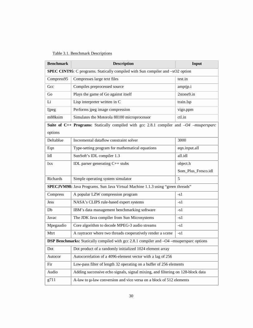
the representative benchmarks used for the study. Table 3.1 lists and describes

the benchmarks that were studied, and their respective inputs. The C benchmarks

from the SPEC95 integer suite are commonly used and are a good point of

reference. The five C++ benchmarks and input files were obtained from

30

Table 3.1. Benchmark Descriptions

Benchmark Description Input

SPEC CINT95: C programs. Statically compiled with Sun compiler and –xO2 option

Compress95 Compresses large text files test.in

Gcc Compiles preprocessed source amptjp.i

Go Plays the game of Go against itself 2stone9.in

Li Lisp interpreter written in C train.lsp

Ijpeg Performs jpeg image compression vigo.ppm

m88ksim Simulates the Motorola 88100 microprocessor ctl.in

Suite of C++ Programs: Statically compiled with gcc 2.8.1 compiler and –O4 –msupersparc

options

Deltablue Incremental dataflow constraint solver 3000

Eqn Type-setting program for mathematical equations eqn.input.all

Idl SunSoft’s IDL compiler 1.3 all.idl

Ixx IDL parser generating C++ stubs object.h

Som_Plus_Fresco.idl

Richards Simple operating system simulator 5

SPECJVM98: Java Programs. Sun Java Virtual Machine 1.1.3 using “green threads”

Compress A popular LZW compression program -s1

Jess NASA’s CLIPS rule-based expert systems -s1

Db IBM’s data management benchmarking software -s1

Javac The JDK Java compiler from Sun Microsystems -s1

Mpegaudio Core algorithm to decode MPEG-3 audio streams -s1

Mtrt A raytracer where two threads cooperatively render a scene -s1

DSP Benchmarks: Statically compiled with gcc 2.8.1 compiler and –O4 –msupersparc options

Dot Dot product of a randomly initialized 1024 element array

Autocor Autocorrelation of a 4096-element vector with a lag of 256

Fir Low-pass filter of length 32 operating on a buffer of 256 elements

Audio Adding successive echo signals, signal mixing, and filtering on 128-block data

g711 A-law to µ-law conversion and vice versa on a block of 512 elements

31

Adpcm 16-bit to 4-bit compression of a speech signal on a 1024-element buffer

Table 3.2. Total Number of Instructions Analyzed and Scheduled by

Tetra for the different benchmarks

Benchmark Instructions Analyzed Instructions Scheduled

SPEC CINT95: C programs

Compress 38.5M 37.1M

Gcc 262.0M 256.7M

Go 510.7M 503.7M

Li 166.6M 159.1M

m88ksim 122.1M 118.3M

Ijpeg 1.4B 1.38B

C++ Programs

Deltablue 40.7M 39.0M

Eqn 47.2M 45.9M

Idl 82.8M 77.8M

Ixx 29.7M 28.7M

Richards 33.0M 31.8M

SPECJVM98

Db 86.8M 84.4M

Javac 198.9M 194.7M

Jess 259.7M 253.8M

Mpegaudio 1.31B 1.31B

Mtrt 1.53B 1.49B

Compress Not Available 1.5B

DSP Benchmarks: C Programs

Dot 41.3M 41.2M

g711 46.4M 44.3M

Autocor 49.4M 49.4M

Fir 42.1M 42.1M

Audio 47.1M 47.0M

32

Adpcm 48.3M 47.8M

the website at the University of Santa Barbara [14]. These benchmarks are

chosen because they have a large dynamic instruction count, and numerous

previous works have studied many of them. The SPEC95 benchmarks are

compiled statically with the Makefiles provided by SPEC. The C++ benchmarks

are also compiled with static linking using g++ (version 2.7.2) as the compiler.

The –O2 and -msupersparc optimization flags are also used. The DSP and media

benchmarks were compiled using gcc with –O4 optimization and –msupersparc

flags.

Table 3.2 gives the number of instructions in each program that are

actually scheduled in the DDG by Tetra. This is less than the total instruction

count of the programs as instructions which do not create any values such as

nops, unconditional jumps etc. are not scheduled in the DDG. For the

experiment, all benchmarks (except the Java program compress) were run to

completion, each program was traced and analyzed dynamically. The dynamic

instruction count of compress is approximately 10 billion and due to time

limitations, we limited the number of instructions that were scheduled to 1.5

billion.

33

4. Results and Analysis

This chapter summarizes the results of this study that characterizes the

selected benchmarks in terms of their instruction level parallelism.

4.1 Dependence Distance

Figure 4.1 shows the dependence distance plots obtained for the C++

program, deltablue, with only RAW dependencies, and RAW, WAW and WAR

dependencies for a window size of 32.

It is seen that as we incorporate more dependencies, the percentage of

instructions having zero dependencies increases. The percentage of instructions

having zero dependencies is 37% when we consider RAW dependencies only and

48% when RAW, WAW and WAR dependencies are taken into consideration.

Also, as we incorporate more dependencies, the percentage of instructions with

dependence distance equal to the window size decreases (19% for RAW only and

9.3% when we consider all RAW, WAW and WAR dependencies). The average

dependence distance decreases from 9.81 when only RAW dependencies are

considered to 5.15 when all dependencies are considered. Evidently, the

dependence distance with only true dependencies gives an upper bound on the

value of dependence distance that can be obtained for that program and window

size. Although the results for only one program for one window size are shown,

all the programs characterized show similar trends for all window sizes.

34

(b)

(a)

Figure 4.1 Dependency Distance for deltablue with (a) only RAW dependencies (b) RAW, WAWand WAR dependencies

35

Table 4.1. Dependence Distance with Window Size = 1024

Benchmark Average Dependence Distance

with Window Size = 1024

Probability of an instruction

having no dependency or

dependency distance ≥ 1024


compress 7.11 0.17

gcc 18.38 0.13

go 28.48 0.15

li 18.27 0.13

m88ksim 13.39 0.16

C++ Programs

deltablue 17.84 0.11

eqn 34.03 0.11

idl 11.53 0.14

ixx 32.68 0.14

richards 8.36 0.15

SPECJVM98

db 16.19 0.099

javac 15.11 0.086

jess 15.32 0.086

mpegaudio 8.03 0.021

mtrt 11.37 0.064


dot 2.84 0.00068

autocor 3.28 0.00052

fir 5.21 0.00056

audio 5.15 0.00061

g711 2.46 0.04491

36

Table 4.1 shows the average dependence distance obtained for the

different programs when only true data dependencies are traced. The window

size is 1024, which means that for each instruction, we examine the previous

1024 instructions to find the most recent data dependence. We present the results

obtained when the window size is 1024 because it was observed that even if the

window size is further increased, the dependence distance distribution does not

change appreciably.

If a program has an average dependence distance, d, an instruction in the

program is on an average, dependent on an instruction that is d instructions

before it in the sequential instruction stream. It is clear from the table that the

C++ and SPECint programs have the highest average dependence distance

followed by the Java and DSP benchmarks. The plots showing the dependence

distance distribution of all the programs with a window size of 1024 are included

in Appendix 1.

4.1.1 Caveats of the Metric

As mentioned previously, the dependence distance metric has some

caveats associated with it. Firstly, the dependence distance is a measure of how

tight the dependencies in a program are. Since we examine the sequential

instruction stream to find the most recent data dependence of an instruction, the

concept of dependent instruction distance is significant only in the context of

37

sequential, in order processors. Secondly, this metric only gives us an idea about

the most recent instruction on which the particular instruction is dependent and

does not reveal anything about the instructions on which the instruction is not

dependent. Thus if an instruction is dependent on an instruction immediately

before it, and does not depend on any of the other 1023 instructions in the

window, the dependence metric does not take it into account. The presence of

short-term dependencies thus overrides the absence of any dependency. This is

evident in the dependence distance obtained for the DSP benchmarks. All these

benchmarks are primarily loops and an examination of the source code suggests

that each iteration of the loop can be scheduled in parallel and therefore,

intuitively, the program should have high parallelism (as illustrated by Tetra).

But, the dependence distance of these programs suggests otherwise. If we look at

the assembly code of these programs, we see that there are a lot of tight

dependencies in the body of the loop. Since we have a large number of iterations,

there are a large number of instructions that have tight dependencies, resulting in

an extremely low average dependence distance. Thus, the dependence distance

metric is more an indicator of the span of dependencies in the program rather

than the amount of inherent parallelism that can be exploited at least as far as out

of order processors are concerned.

38

For example, consider the following extract from the main loop of the

assembly code corresponding to the DSP benchmark, fir :

LL9:

I0: add %i5,%g4,%g2

I1: sll %g2,1,%g2

I2: sll %i5,1,%i0

I3: ldsh [%o7+%g2],%g3

I4: ldsh [%i1+%i0],%g2

I5: smul %g3,%g2,%g3

I6: add %i5,1,%i5

I7: cmp %i5,%i3

I8: bl .LL9

I9: add %g1,%g3,%g1

Instructions I1, I5, I7 and I8 have dependence distances of 0 since they are

dependent on the immediate preceding instruction. Although the other

instructions do not have dependencies within the current iteration, they do have

dependencies on instructions in the previous iteration. For example I0 will have a

dependency on I6 of the previous iteration. These intra and inter iteration

dependencies greatly lower the dependence distance of the program. In the case

of fir , 40.4% of instructions have a dependence distance of 0, 19.5% have

dependence distance of 1, another 19.5% have dependence distance of 3, 19% of

instructions have dependence distance of 5 and 9 respectively (9.5% each), and

only 0.06% of instructions have a dependence distance of 1024. The other DSP

39

programs also exhibit similar behavior. This distribution clearly explains the low

dependence distance exhibited by these benchmarks.

4.2 Available Parallelism

Tables 4.2 to 4.7 show the critical path length and the available program

parallelism obtained using the DDG technique in Tetra when the Machine Level

Parallelism(MLP) is varied from infinity down to 8. The critical path length is

identical to the height of the scheduled DDG and gives the absolute minimum

number of steps required to evaluate the operations in the scheduled DDG. The

Machine Level Parallelism (MLP), as mentioned previously, is the maximum

number of instructions that the machine is capable of scheduling in a single cycle

(each level in the DDG represents a cycle). When MLP is infinity (i.e. the same

size as the trace), the number of instructions that can be scheduled is limited only

by the inherent program dependencies. Since we consider only true dependencies

(or RAW dependencies) while scheduling instructions, this is the absolute limit of

parallelism that can potentially be exploited from that program.

We measure the available parallelism in terms of the average number of

instructions that can be scheduled per cycle. Since this represents a rate, we use

the harmonic mean to obtain the central tendency of the observations [16]. The

40

Table 4.2. Available ILP with MLP = Infinity

Benchmark Critical Path Length Available ILP


compress 140,104 265.01

gcc 2,786,390 92.14

go 6,010,319 83.81

li 2,194,937 72.48

m88ksim 887,805 133.36

ijpeg 163,453 8465.51

C++ Programs

deltablue 143995 270.97

eqn 168929 272.09

idl 281075 277.01

ixx 257532 111.71

richards 254036 125.57

SPECJVM98

db 2067947 41.06

javac 7755231 25.13

jess 11134853 22.83

mpegaudio 85152326 15.39

mtrt 94130779 15.82

compress 125558591 11.95


dot 5003 8239.82

g711 4003 11064.15

autocor 4102 12057.35

fir 2222 18964.54

audio 2222 21164.94

adpcm 1178180 40.59

41

harmonic mean is given by the following equation where Ri is the ith rate and n is

the number of observations.

Table 4.2 illustrates that with infinite MLP, the average ILP (in terms of

the harmonic mean) is highest for the DSP benchmarks, being about 239.7. The

Java benchmarks exhibit the least available parallelism with an average of about

18.76. The SPECint and C++ programs fall in between with an average ILP of

approximately 125.07 and 179.27 respectively.

The extremely low ILP of the Java programs, even with no other control

or machine constraints, can be attributed to the stack-based implementation of

the Java Virtual Machine (JVM). This imposes a strict ordering on the execution

of the bytecodes. Since we are running the Java programs in interpreted mode, all

accesses to the Java stack are translated into read and write operations to

memory, each one of them being dependent on the corresponding operations of

the previous bytecode (running the Java programs in a JIT environment will

result in the use of registers to pass values between bytecodes, thus avoiding the

stack dependencies). This is supported by the behavior of the compress

benchmark, which is present in both the SPECint 95 and SPECJVM suites. Both

∑=

=

n

i iR

neanharmonic m

1

1

42

are text compression programs and the Java version is a Java port of the integer

benchmark from CPU95. It can be seen that with an MLP of infinity, the CPU95

compress benchmark has the highest ILP among all the SPECint benchmarks

while the Java compress program has the least ILP among the SPECJVM

benchmarks. The algorithm in both cases is essentially the same and thus, this

illustrates the impact of the programming language and paradigm on the available

program parallelism.

Among the C programs, the DSP benchmarks have a higher parallelism

than the SPECint benchmarks. This is obviously due to the fact that these

benchmarks consist of loops, which operate over large data arrays. With infinite

MLP, most of the instructions in each iteration can be scheduled in parallel thus

giving an extremely high value for the available ILP. The only program in this

category that does not exhibit an extremely high ILP is adpcm. The adpcm

benchmark is an Adaptive Differential Pulse Code Modulation (ADPCM) codec

which, instead of quantizing the speech signal directly, quantizes the difference

between the speech signal and a prediction that has been made of the speech

signal. Thus, the value of each sample is computed using the previous sample

with the result that the algorithm itself has very little parallelism. The resulting

assembly code has tight inter-iteration dependencies. Moreover, most of the

instructions in the body of the loop also have dependencies among themselves

43

and as a result, the body of the loop is highly sequential and very little can be

scheduled in parallel.

Tables 4.3 through 4.7 illustrate the available ILP obtained using Tetra

when we restrict the MLP to 128, 64, 32, 16 and 8 respectively. It is seen that

the relative trend among the different categories of programs remains the same in

each case with the C and C++ programs exhibiting higher ILP than the Java

programs. However, the variation of ILP across the different suites of programs

decreases as the MLP is decreased. Also, the benchmarks in each category do not

show as much variation among themselves as in Table 4.2.

This clearly illustrates the impact of MLP on the overall available ILP.

For programs which have a very high available ILP with infinite MLP, there is a

substantial drop in ILP when the MLP is restricted. Obviously, in these cases,

MLP is the factor which limits the overall available parallelism. This is especially

true with the media benchmarks, all of which (except adpcm) exhibit an ILP close

to the maximum available MLP. With MLP of 128 and 64, the SPECint

benchmarks have an average available parallelism of 71.27 and 44.27

respectively, while the corresponding values for the C++ benchmarks are 63.51

and 45.06.

44

Table 4.3. Available ILP with MLP = 128



compress 563457 65.89

gcc 4415197 58.15

go 7172458 70.23

li 2267860 70.15

m88ksim 1133722 104.43

ijpeg 19255478 71.86

C++ Programs

deltablue 350632 111.28

eqn 1056504 43.51

idl 1226273 63.49

ixx 378286 76.05

richards 569671 55.99

SPECJVM98

db 2518294 33.7

javac 8911040 21.89

jess 12216964 20.78

mpegaudio 86309302 15.19

mtrt 103778323 14.38

compress 126211222 11.88

DSP Benchmarks: C programs

dot 324334 127.10

g711 351911 125.86

autocor 393330 125.62

fir 338469 124.35

audio 400556 117.41

adpcm 1181576 40.48

45




compress 986207 37.65

gcc 6294134 40.79

go 10323869 48.79

li 3372490 47.17

m88ksim 2596460 45.59

ijpeg 28816774 48.01

C++ Programs

deltablue 645184 60.48

eqn 1210907 37.96

idl 1611762 48.31

ixx 560612 51.32

richards 890124 35.84

SPECJVM98

db 2958008 28.55

javac 9822431 19.82

jess 12991292 19.54

mpegaudio 89582094 14.63

mtrt 106145169 14.06

compress 128415995 11.68


dot 648381 63.58

g711 708340 62.53

autocor 784664 62.96

fir 666731 63.12

audio 779241 60.35

adpcm 1184615 40.37

46




compress 1695440 21.9

gcc 10042793 25.56

go 18476688 27.26

li 6276137 25.35

m88ksim 5505974 21.50

ijpeg 48623241 28.46

C++ Programs

deltablue 1267057 30.79

eqn 1731742 26.54

idl 2680517 29.05

ixx 1068546 26.92

richards 1284616 24.83

SPECJVM98

db 4319985 19.54

javac 12522061 15.55

jess 15698918 16.17

mpegaudio 101876876 12.86

mtrt 115481404 12.92

compress 130929990 11.46


dot 1295414 31.82

g711 1414550 31.31

autocor 1551034 31.86

fir 1336029 31.5

audio 1492249 31.52

adpcm 1977172 24.19

47




compress 2715042 13.68

gcc 18417667 13.94

go 35699731 14.11

li 11167026 14.25

m88ksim 10680439 11.09

ijpeg 94285745 14.67

C++ Programs

deltablue 2575048 15.15

eqn 3241477 14.18

idl 5337553 14.59

ixx 2079613 13.83

richards 2314781 13.78

SPECJVM98

db 7315803 11.59

javac 18257758 10.67

jess 23046533 11.02

mpegaudio 129590638 10.11

mtrt 145170690 10.26

compress 155203799 9.66


dot 2594273 15.91

g711 2880640 15.39

autocor 3103241 15.94

fir 2685676 15.69

audio 3004963 15.67

adpcm 3566941 13.42

48




compress 5351993 6.94

gcc 35347266 7.26

go 70458915 7.15

li 21303375 7.47

m88ksim 18354950 6.45

ijpeg 186008654 7.44

C++ Programs

deltablue 5356366 7.28

eqn 6191092 7.42

idl 10284540 7.57

ixx 3990388 7.2

richards 4219721 7.56

SPECJVM98

db 12509764 6.75

javac 29231382 6.66

jess 37956012 6.69

mpegaudio 180376177 7.27

mtrt 220761403 6.76

compress 214896732 6.98


dot 5177328 7.97

g711 5855045 7.57

autocor 7421899 6.66

fir 6319308 6.67

audio 6938488 6.79

adpcm 6595073 7.26

49

In the case of programs that do not show high parallelism even with

infinite window size, such as the Java programs and the DSP benchmark, adpcm,

the available ILP does not change much as we decrease MLP, until the MLP is

restricted to a value that is less than the maximum available parallelism, ILPmax

(i.e. the ILP with infinite MLP). For these programs, even when MLP is infinity,

the inherent program dependencies limit the number of instructions that can be

scheduled per cycle. Once the MLP is increased to a value that is greater than

ILPmax, the ILP does not increase appreciably even when the MLP is further

increased.

For example, adpcm shows an available ILP between 40 and 41 when the

MLP is infinity, 128 or 64. It is only when the MLP is less than 40 (32, 16 or 8)

that the available ILP changes because in these cases, the available ILP is limited

by the available MLP. Similarly, the ILP for the Java program compress does not

vary much when MLP is varied from infinity down to 16.

It is seen that when the MLP is 8 or 16, all the different programs show

comparable ILP, although the Java programs still remain at the lower end of the

spectrum. With an MLP of 16, the mean ILP is 13.51 for the SPECint

benchmarks, 14.28 for the C++ programs, 10.51 for the Java programs and 15.28

for the DSP benchmarks. When the MLP is 8, the mean values are is 7.1 for the

SPECint benchmarks, 7.4 for the C++ programs, 6.85 for the Java programs and

50

7.12 for the DSP benchmarks. Thus, with values of MLP such as 8 and 16, the

overall available ILP is limited by the MLP, irrespective of the programming

language. Thus, to observe and compare the differences in the inherent available

parallelism of different programs, we need to make MLP as large as possible. The

larger the MLP, the more marked will be the variation in the observable ILP.

The average available parallelism (in terms of the harmonic mean of the

observations) of the four different suites of programs for different window sizes

is summarized in Figure 4.2.

Tables 4.8 and 4.9 illustrate the available ILP when MLP is 8 and 32

respectively, with no branch prediction. All the programs have an average

available ILP of around 2 with MLP = 8 and this does not change appreciably

0

50

100

150

200

250

300

MLP =

Infin

ity

MLP =

128

MLP = 64

MLP = 32

MLP = 16

MLP =

8

Ava

ilabl

e P

aral

lelis

m

SPECint

C++

SPECJVM

DSP

Figure 4.2 Average available parallelism of SPECint, C++, SPECJVM andDSP benchmarks for different values of MLP

51

Table 4.8. Available ILP with MLP = 8 and no branch prediction



compress 15818822 2.35

gcc 138885673 1.85

go 75354853 2.01

li 84871231 1.87

m88ksim 53936861 2.19

ijpeg 420699229 3.29

C++ Programs

deltablue 17486679 2.23

eqn 24967904 1.84

idl 42830788 1.82

ixx 14375325 2.01

richards 18509928 1.72

SPECJVM98

db 39394824 2.14

javac 88480846 2.19

jess 11262263 2.26

mpegaudio 367269435 3.57

mtrt 700407903 2.13

compress 434274925 3.45

DSP Benchmarks

dot 15568238 2.65

g711 24777158 1.79

autocor 14940445 3.31

fir 13111319 3.21

audio 15455439 3.05

adpcm 30938072 1.55

52

Table 4.9. Available ILP with MLP = 32 and no branch prediction



compress 15602465 2.38

gcc 138081577 1.86

go 248020645 2.03

li 84410418 1.88

m88ksim 53839550 2.19

ijpeg 355998522 4.12

C++ Programs

deltablue 17148661 2.28

eqn 24529501 1.87

idl 42651095 1.83

ixx 14079414 2.04

richards 18230571 1.75

SPECJVM98

db 38977756 2.17

javac 87382752 2.23

jess 1112528287 2.28

mpegaudio 359905400 3.64

mtrt 699535053 2.13

compress 424828215 3.53

DSP Benchmarks

dot 15567639 2.65

g711 24776560 1.79

autocor 14939846 3.31

fir 13110721 3.21

audio 15454841 3.05

adpcm 30937476 1.55

53

when the MLP is increased to 32. This shows the impact of control dependencies

on available parallelism. Even with infinite functional units and an MLP of 32, the

presence of control dependencies limit the available program parallelism to about

2. This illustrates the importance of branch prediction techniques to maximally

exploit available parallelism.

54

5. Conclusion

The characterization of a program or benchmark in terms of its intrinsic

properties is of fundamental importance in the analysis and evaluation of system

performance and design decisions, independent of system parameters. One of the

most important program properties that is regularly exploited in modern

microprocessors is the available instruction level parallelism. In this study, we

examine the limits to instruction level parallelism in some modern representative

applications. Instead of confining the study to the SPEC95 applications, current

applications such as C++ programs, Java programs and a set of DSP and media

were benchmarks studied. We analyzed two different metrics in terms of which

the available parallelism can be characterized, independent of machine

implementation details. As such, we focus on logical limits, rather than on

implementation issues and towards this end, we assume an ideal machine

configuration.

Our results illustrate there is significant parallelism in applications which

are traditionally thought to be sequential. However, this parallelism can be

effectively exploited only if the processor can accurately look ahead arbitrarily far

into the dynamic instruction stream. This type of parallelism is referred to as

“distant parallelism” which is the possibility to execute instructions which are

hundreds of thousands of instructions away from each other. Thus, our study

55

emphasizes the importance of techniques which attempt to exploit control

independence to extract the distant parallelism [14].

We also found that however high the inherent instruction parallelism, a

limited machine level parallelism considerably limits the overall available

parallelism. Our study also indicated that among the different categories of

programs that we examined, the Java programs have considerably less parallelism

than the C and C++ programs. The available parallelism ranges from 11 to 21000

in the various benchmarks that we examined, with harmonic means of 125.07 for

the C benchmarks, 179.27 for the C++ benchmarks, 18.76 for the Java programs

and 239.7 for the DSP benchmarks. The extremely low parallelism of the Java

appliocations can be attributed to the stack based implementation of the JVM and

the fact that we run the programs in interpreted mode. However, with a limited

MLP, all programs exhibit comparable parallelism irrespective of the

programming language as in this case, the available ILP is limited by the MLP.

Our results further strengthen the importance of branch prediction to

remove effect of control dependencies and to maximally exploit instruction

parallelism. Obtaining the parallelism demonstrated in this study requires both

register and memory renaming, perfect control flow and memory disambiguation.

Analysis of the ILP characteristics of current workloads will provide

valuable hints that will help in the design of both future workloads and future

56

processors. Despite the fact that quantitative analysis methods are expensive with

respect to both time and resources, such studies are going to be essential in

understanding the dynamics of program execution on future architectures,

especially when we consider the increasing complexity of modern day computer

systems.

57

Appendix A

Dependence Distance Distribution Plots

The dependence distance distribution plots for the C, C++, Java and

media benchmarks are included. Although the analysis was carried out with a

window size of 1024, only the lower range of values are shown for clarity. In all

the cases, the probability is almost zero for all the remaining values of

dependency distance,except for 1024, the window size. The percentage of

instructions which have dependency distance 1024 are given in Table 4.1 on pp.

29.

58

Figure A1 Dependence distance distribution of compress with window size1024

Figure A2 Dependence distance distribution of gcc with window size 1024

59

Figure A3 Dependence distance distribution of go with window size 1024

Figure A4 Dependence distance distribution of li with window size 1024

60

Figure A5 Dependence distance distribution of m88ksim with window size 1024

Figure A6 Dependence distance distribution of deltablue with window size 1024

61

Figure A7 Dependence distance distribution of eqn with window size 1024

Figure A8 Dependence distance distribution of idl with window size 1024

62

Figure A9 Dependence distance distribution of ixx with window size 1024

Figure A10 Dependence distance distribution of richards with window size1024

63

Figure A11 Dependence distance distribution of db with window size 1024

Figure A12 Dependence distance distribution of javac with window size 1024

64

Figure A13 Dependence distance distribution of jess with window size 1024

Figure A14 Dependence distance distribution of mpegaudio with window size 1024

65

Figure A15 Dependence distance distribution of mtrt with window size 1024

Figure A16 Dependence distance distribution of dot with window size 1024

66

Figure A17 Dependence distance distribution of autocor with window size 1024

Figure A18 Dependence distance distribution of fir with window size 1024

67

Figure A19 Dependence distance distribution of audio with window size 1024

Figure A20 Dependence distance distribution of g711 with window size 1024

68

References

[1] T. M. Austin and G. S. Sohi, “TETRA: Evaluation of Serial ProgramPerformance on Fine-Grain Parallel Processors”, University of Wisconsin -Madison Technical Report # 1162, July 1993.

[2] D. B. Noonburg and J. P. Shen, “A Framework for Statistical Modeling ofSuperscalar Processors”, Proceedings of HPCA-3, pp. 298-309, 1997.

[3] T. M. Austin and G. S. Sohi, “Dynamic Dependency Analysis of OrdinaryPrograms”, Proceedings of the 19th Annual International Symposium onComputer Architecture, pp. 342-351, May 1992.

[4] M. A. Postiff et. al, “The Limits of Instruction Level Parallelism in SPEC95Applications”, Proceeding of the 3rd Workshop on Interaction BetweenCompilers and Computer Architecture (INTERACT-3), October 1998.

[5] D. W. Wall, “Limits of Instruction Level Parallelism”, Technical ReportDEC-WRL-93-6, Digital Equipment Corporation, Western Research Lab,November 1993.

[6] M. Butler et. al, “Single Instruction Parallelism Is Greater Than Two”,Proceedings of ISCA-18, Volume 19, pp. 276-286, June 1991.

[7] N. P. Jouppi and D. W. Wall, “Available Instruction Level Parallelism forSuperscalar and Superpipelined Machines”, Proceedings of ASPLOS-3, Volume24, pp. 272-282, May 1989.

[8] P. K. Dubey et al., “Instruction Window Size Trade-offs and ProgramParallelism”, IEEE Transactions on Computers, 43(4):431-442, April 1994.

[9] G. S. Tjaden and M. J. Flynn, “Detection and Parallel Execution ofIndependent Instructions”, Journal of the ACM, 19(10):889-895, October 1970.[9]. M. Johnson, Superscalar Microprocessor Design, NJ: P T R Prentice Hall,1991.

[10] R. Sathe and M. Franklin, “Available Parallelism with Data ValuePrediction”, Proceedings of HiPC-98 (International Conference on HighPerformance Computing), pp. 194-201, April 1998.

69

[11] L. K. John, P. Vasudevan, and J. Sabarinathan, “WorkloadCharacterization:Motivation, Goals and Methodology”, in WorkloadCharacterization : Methodology and Case Studies, pp. 3-14, IEEE ComputerSociety, 1999.

[12] R.Radhakrishnan, J. Rubio and L. John, “Characterization of JavaApplications at Bytecode and Ultra-SPARC Machine Code Levels”, Proceedingsof IEEE International Conference on Computer Design, pp. 281-284, October1999

[13] R. Radhakrishnan and L. John, “Execution Characteristics of ObjectOriented Programs on the UltraSPARC-II”, Proceedings of the 5th InternationalConference on High Performance Computing, pp. 202-211, December 1998.

[14] A. Bhowmik and M. Franklin, “A Characterization of Control IndependenceIn Programs”, Proceedings of the Second Workshop on WorkloadCharacterization, October 1999.

[15] T.-Y. Yeh and Y. N. Patt, “Alternative Implementations of Two-LevelAdaptive Branch Prediction”, Proceedings of ISCA-19, pp. 124-135, May 1992.

[16] H. Cragon, Computer Architecture and Implementation, CambridgeUniversity Press, In press.

[17] M. Johnson, Superscalar Microprocessor Design, NJ: P T R Prentice Hall,1991.

[18] D.Patterson and J.Hennessy, Computer Architecture: A QuantitativeApproach, 2nd ed., Morgan Kaufmann Publishers, Inc., San Francisco, CA, 1996.

[19]. “Introduction to Shade,” Shade User’s manual, Sun Microsystems, 1993.

[20]. R. Cmelik and D. Keppel, “Shade, a fast instruction-set simulator forexecution profiling,” Sun Microsystems Inc., Technical Report SMLI TR-93-12,1993.

[21]. D. Weaver and T. Germond, ed., The SPARC Architecture Manual, version9, Prentice Hall Inc., Englewood Cliffs, NJ 1994.

[22] Sun Microsystems, Inc., Introduction to Spixtools, Version 5.33A, 1997.

70

[23] A C++ benchmark suite, http://www.cs.ucsb.edu/oocsb/benchmarks.

71

VITA

Jyotsna Sabarinathan, the daughter of Renu Sabarinathan and

Dr. K. Sabarinathan was born in Long Island, New York on February 20th, 1976.

After graduating from Mar Ivanios College, Trivandrum, India, Jyotsna entered

the Electronics and Communication Engineering program at the Govt. College of

Engineering, Trivandrum, India. She graduated in December 1997, and entered

the Graduate School at The University of Texas at Austin on a Microelectronics

and Computer Fellowship to pursue graduate studies in August 1998.

Permanent Address: 4912 Weatherhill Rd SW

Rochester, MN 55902

This report was typed by the author.

A Study of Instruction Level Parallelism in Contemporary ... · parallelism can be quantified,...

Documents

Transcript of A Study of Instruction Level Parallelism in Contemporary ... · parallelism can be quantified,...