A Study of Fuzzy Linear Regression -...
23
A Study of Fuzzy Linear Regression Dr. Jann-Huei Jinn Department of Statistics Grand Valley State University Allendale, Michigan, 49401 and Dr. Chwan-Chin Song and Mr. J. C. Chao Department of Applied Mathematics National Cheng-Chi University Taipei, Taiwan, R.O.C. 1. Introduction We often use regression analysis to model the relationship between dependent (response) and independent (explanatory) variables. In traditional regression analysis, residuals are assumed to be due to random errors. Thus, statistical techniques are applied to perform estimation and inference in regression analysis. However, the residuals are sometimes due to the indefiniteness of the model structure or imprecise observations. The uncertainty in this type of regression model becomes fuzziness, not random. Since Zadeh (1965) proposed fuzzy sets, fuzziness has received more attention and fuzzy data analysis has become increasingly important. In order to consider the fuzziness in regression analysis, Tanaka et al. (1982) first proposed a study of fuzzy linear regression (FLR) model. They considered the parameter estimations of FLR models under two factors, namely the degree of the fitting and the vagueness of the model. The estimation problems were then transformed into linear programming (LP) based on these two factors. Since the measure of best fit by residuals under fuzzy consideration is not presented in Tanaka’s approach, Diamond (1988) proposed the fuzzy least-squares approach, which is a fuzzy extension of the ordinary least squares based on a new defined distance on the space of fuzzy numbers. In general, the fuzzy regression methods can be roughly divided into two categories. The first is based on Tanaka’s LP approach. The second category is based on the fuzzy least-squares approach. In section 2, we introduced the fuzzy number and its operation, a simple distance formula, two fuzzy linear regression models and their least squares estimates. In section 3, we introduced LR type fuzzy number and nonsymmetrical doubly linear adaptive fuzzy regression model, Yang and Ko’s distance formula, and least squares estimates which relate to membership functions. In section 4, we applied traditional methods of detecting possible outliers and influence points to derive the leverage values, residuals and Cook distance formula for the fuzzy linear regression models..
Transcript of A Study of Fuzzy Linear Regression -...
A Study of Fuzzy Linear Regression
Dr. Jann-Huei Jinn
Department of Statistics
Grand Valley State University
Allendale, Michigan, 49401
and
Dr. Chwan-Chin Song and Mr. J. C. Chao
Department of Applied Mathematics
National Cheng-Chi University
Taipei, Taiwan, R.O.C.
1. Introduction
We often use regression analysis to model the relationship between dependent
(response) and independent (explanatory) variables. In traditional regression analysis,
residuals are assumed to be due to random errors. Thus, statistical techniques are applied
to perform estimation and inference in regression analysis. However, the residuals are
sometimes due to the indefiniteness of the model structure or imprecise observations. The
uncertainty in this type of regression model becomes fuzziness, not random. Since Zadeh
(1965) proposed fuzzy sets, fuzziness has received more attention and fuzzy data analysis
has become increasingly important.
In order to consider the fuzziness in regression analysis, Tanaka et al. (1982) first
proposed a study of fuzzy linear regression (FLR) model. They considered the parameter
estimations of FLR models under two factors, namely the degree of the fitting and the
vagueness of the model. The estimation problems were then transformed into linear
programming (LP) based on these two factors. Since the measure of best fit by residuals
under fuzzy consideration is not presented in Tanaka’s approach, Diamond (1988)
proposed the fuzzy least-squares approach, which is a fuzzy extension of the ordinary
least squares based on a new defined distance on the space of fuzzy numbers. In general,
the fuzzy regression methods can be roughly divided into two categories. The first is
based on Tanaka’s LP approach. The second category is based on the fuzzy least-squares
approach.
In section 2, we introduced the fuzzy number and its operation, a simple distance
formula, two fuzzy linear regression models and their least squares estimates.
In section 3, we introduced LR type fuzzy number and nonsymmetrical doubly linear
adaptive fuzzy regression model, Yang and Ko’s distance formula, and least squares
estimates which relate to membership functions.
In section 4, we applied traditional methods of detecting possible outliers and
influence points to derive the leverage values, residuals and Cook distance formula for
the fuzzy linear regression models..

In section 5, we used the theoretical results in the previous chapters to analyze the
Tanaka’s (1987) data.
The derivation of some important formulas is given in appendices.
2. Introduction to Fuzzy Linear Regression
2.1 Fuzzy �umber and Its Operation
Fuzzy data is a natural type of data, like non-precise data or data with a source of
uncertainty not caused by randomness. This kind of data is easy to find in natural
language, social science, psychometrics, environments and econometrics, etc. Fuzzy
numbers have been used to represent fuzzy data. These are also used to model fuzziness
of data.
Let ℜ be a one-dimensional Euclidean space with its norm denoted by . . A fuzzy
number is an upper semicontinuous convex function F: ℜ → [0,1] with { }1)( =ℜ∈ xFx
non-empty. In other words, a fuzzy number A is defined as a convex normalized fuzzy
set of the real line ℜ so that there exists exactly one ox ∈ ℜ with F( ox )=1, and its
membership F(x) is piecewise continuous.
Definition 2.1 (Zimmermann [pp.62-63])
Let L (and R) be decreasing, shape functions from +ℜ to [0,1] with L(0)=1; L(x)<1
for all x>0; L(x)>0 for all x<1; L(1)=0 for all x and L(+∞ )=0). Then a fuzzy number A is called of LR-type if for m, α >0, 0>β in ℜ ,
A(x)=
≥
−
≤
−
,
,
mxmx
R
mxxm
L
β
α where m is called the center (mean or mode)value of A
and α and β are called left and right spreads, respectively. Symbolically, A is denoted by ( )LRm βα ,, . If α = β , A=(m,α , α ) LR is called symmetrical fuzzy number, denoted by A=(m, α ) LR . For instance, the algebraic and geometric characteristics of the membership function of the more utilized LR fuzzy number, the triangular fuzzy
number, are shown in the following:
A(x)=
+≤≤−
−
≤≤−−
−
,1
,1
αβ
αα
mxmmx
mxmxm
Another example, the exponential fuzzy number, its membership function
A(x)=
≥
−−
≤
−−
,exp
,exp
mxs
mx
mxs
xm
n
n
where s is the spread.
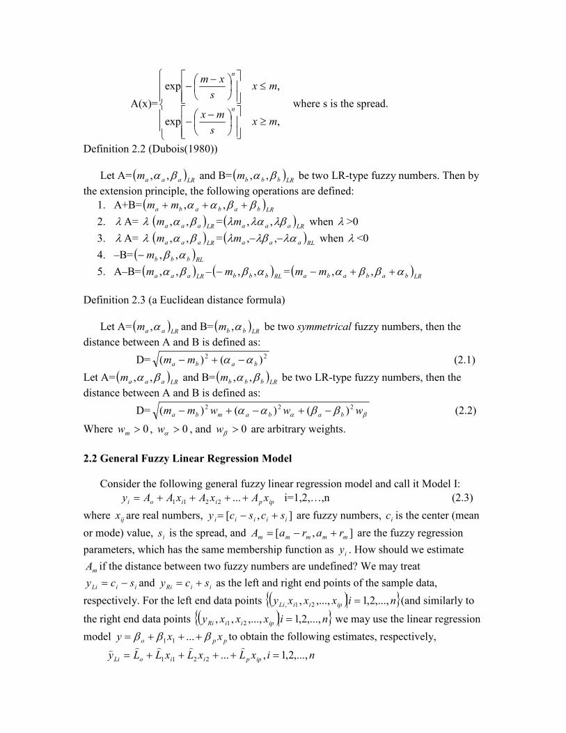
Definition 2.2 (Dubois(1980))
Let A= ( )LRaaam βα ,, and B= ( )
LRbbbm βα ,, be two LR-type fuzzy numbers. Then by
the extension principle, the following operations are defined:
1. A+B= ( )LRbababa mm ββαα +++ ,,
2. λ A= λ ( )LRaaam βα ,, = ( )
LRaaam λβλαλ ,, when λ >0
3. λ A= λ ( )LRaaam βα ,, = ( )
RLaaam λαλβλ −− ,, when λ <0
4. –B= ( )RLbbbm αβ ,,−
5. A–B= ( )LRaaam βα ,, – ( )
RLbbbm αβ ,,− = ( )LRbababa mm αββα ++− ,,
Definition 2.3 (a Euclidean distance formula)
Let A= ( )LRaam α, and B= ( )
LRbbm α, be two symmetrical fuzzy numbers, then the
distance between A and B is defined as:
D= 22 )()( baba mm αα −+− (2.1)
Let A= ( )LRaaam βα ,, and B= ( )
LRbbbm βα ,, be two LR-type fuzzy numbers, then the
distance between A and B is defined as:
D= βα ββαα wwwmm babamba
222 )()()( −+−+− (2.2)
Where 0>mw , 0>αw , and 0>βw are arbitrary weights.
2.2 General Fuzzy Linear Regression Model
Consider the following general fuzzy linear regression model and call it Model I:
ippiioi xAxAxAAy ++++= ...2211 i=1,2,…,n (2.3)
where ijx are real numbers, ],[ iiiii scscy +−= are fuzzy numbers, ic is the center (mean
or mode) value, is is the spread, and ],[ mmmmm raraA +−= are the fuzzy regression
parameters, which has the same membership function as iy . How should we estimate
mA if the distance between two fuzzy numbers are undefined? We may treat
iiLi scy −= and iiRi scy += as the left and right end points of the sample data,
respectively. For the left end data points ( ){ }nixxxy ipiiLi ,...,2,1,...,, 21, = (and similarly to
the right end data points ( ){ }nixxxy ipiiRi ,...,2,1,...,,, 21 = we may use the linear regression
model ppo xxy βββ +++= ...11 to obtain the following estimates, respectively,
nixLxLxLLy ippiioLi ,...,2,1,...2211 =++++=)))))

nixRxRxRRy ippiioRi ,...,2,1... ,2211 =++++=)))))
Then, [ ]mmmmm raraA)))))
+−= , where 2
mmm
RLa
))) +
= , 2
mm
m
LRr
))
) −= .
Using this way to estimate the regression parameters, mA , didn’t consider the
advantage of using the membership function to describe the data. The fuzzy concept were
not used in the estimation of parameters. In order to obtain more appropriate estimates of
fuzzy regression parameters, mA , the least squares method and the distance between two
fuzzy numbers should be considered.
Based on the definition 2.3, we can use ordinary least-squares method to estimate the
fuzzy parameters in the general fuzzy linear regression model ((2.3), Model I). Assuming
that iy = ),( ii sc and ),( mmm raA = have same membership function, after appropriate
translation, we can make all of 0>ijx . Then (2.3) can be expressed as
ipppiiooii xraxraxrarasc ),(...),(),(),(),( 222111 ++++=
According to the Euclidean distance formula of (2.1), the least-squares estimates of ia
and ir are the values of ia , ir which minimize the value of 2D where
2D = [ ]∑=
+++−++++−n
i
ippioiippioi xrxrrsxaxaac1
2
11
2
11 ))...(())...((
Let vr denote the length of vector v
r, then by using vector and matrix expressions
2D can be rewritten as 2D =2
Ca −Χ +2
Sr −Χ where Χ is a )1( +× pn design
matrix, )',...,,( 1 po aaaa = , )',...,,( 1 po rrrr = , )',...,,( 21 ncccC = , and )',...,,( 21 nsssS = .
Let 02
=∂∂a
D and 0
2
=∂
∂r
Dthen the solutions of a and rwhich minimize 2D are as
follows: Ca ')'(ˆ 1ΧΧΧ= −
Sr ')'(ˆ 1ΧΧΧ= − (2.4)
The above method used regression with respect to center and spread. The estimation
results are not related to the membership functions. But, in the later real data analyses,
this method provided better results in the estimation of fuzzy parameter values.
2.3 Symmetrical Doubly Linear Adaptive Fuzzy Regression Model
Under the structure of model I, if we use the Euclidean distance formula and the least-
squares method to do linear regression with respect to center and spread respectively,
then the estimates show that the centers and spreads are not related. But, D’Urso and
Gastaldi (2000) think that the dynamic of the spreads is somehow dependent on the
magnitude of the (estimated) centers. Therefore, they proposed the doubly linear adaptive
fuzzy regression model (call it Model II) to obtain the parameter estimates.

They considered symmetrical fuzzy numbers with triangular membership function.
Where a fuzzy number, iy = ),( ii sc , is completely identified by the two parameters c
(center) and s (left and right spread). Model II is defined as follows:
cCC ε+= * aC Χ=* (2.5)
sSS ε+= * dbCS 1** += (2.6)
whereΧ is a )1( +× pn matrix containing the input variables (data
matrix), )',...,,( 1 po aaaa = is a column vector containing the regression parameters of the
first model (referred to as core regression model), )',...,,( 21 ncccC = and aC Χ=* are the
vector of the observed centers and the vector of the interpolated centers, respectively,
both having dimensions 1×n , and )',...,,( 21 nsssS = and *S are the vector of the
assigned spreads and the vector of the interpolated spreads, respectively, both having
dimension 1×n , 1 is a 1×n -vector of all 1's, b and d are the regression parameters for
the second regression model (referred to as spread regression model).
Apparently, the above model is based on two linear models. The first one interpolates
the centers of the fuzzy observations, the second one yields the spreads, by building
another linear model over the first one. Observe that predictive variables X are taken into
consideration in Eq. (2.6) through the observed centers. The model is hence capable to
take into account possible linear relations between the size of the spreads and the
magnitude of the estimated centers. This is often the case in real world applications,
where dependence among centers and spreads is likely (for instance, the uncertainty or
fuzziness with a measurement could depend on its magnitude).
D’Urso and Gastaldi used the Euclidean distance formula of (2.1) and the least-
squares method to obtain the estimates of a ,b and d such that the value of 2D is
minimized, where
2D =2
*2
* SSCC −+−
= 22 1''21'2'2')1('''2' ndbdadSabSSSbaaaCCC +Χ+−Χ−++ΧΧ+Χ−
Let 02
=∂∂a
D, 0
2
=∂∂b
D and 0
2
=∂∂d
D, they obtained the following equations:
02
=∂∂a
D= bdSbbaC 1'')1('' 2 Χ+Χ−+ΧΧ+Χ−
02
=∂∂b
D= daaSaba 1''''' Χ+Χ−ΧΧ
02
=∂∂d
D= ndbaS +Χ+− 1''1' (2.7)
Based on the equations in (2.7), they obtained the following least-squares iterative
solutions of a ,b and d :
a = ))1(')'(()1(
1 1
2bdSbC
b−+ΧΧΧ
+−
b = )1'''()''( 1 daaSaa Χ−ΧΧΧ −
d = )1''1'(1
baSn
Χ− (2.8)
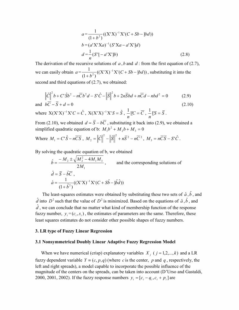
The derivation of the recursive solutions of a ,b and d : from the first equation of (2.7),
we can easily obtain a = ))1(')'(()1(
1 1
2bdSbC
b−+ΧΧΧ
+− , substituting it into the
second and third equations of (2.7), we obtained:
02ˆˆ'ˆ'ˆ 22
222
=−++−−−+ nbddCnbdSnbSCSdbCnbSCbC (2.9)
and 0=+− dSCb (2.10)
where CC ˆ')'( 1 =ΧΧΧΧ − , SS ˆ')'( 1 =ΧΧΧΧ − , CCn
='11
, SSn
='11
.
From (2.10), we obtained CbSd −= , substituting it back into (2.9), we obtained a
simplified quadratic equation of b: 032
2
1 =++ MbMbM
Where SCnSCM −= ˆ'1 , 2222
2ˆˆ CnSnSCM −+−= , CSSCnM ˆ'3 −= .
By solving the quadratic equation of b, we obtained
1
31
2
22
2
4ˆM
MMMMb
−±−= , and the corresponding solutions of
CbSd ˆˆ −= ,
))ˆˆ1ˆ(')'(()ˆ1(
1ˆ 1
2dbbSC
ba −+ΧΧΧ
+= −
The least-squares estimates were obtained by substituting these two sets of a , b , and
d into 2D such that the value of 2D is minimized. Based on the equations of a , b , and
d , we can conclude that no matter what kind of membership function of the response
fuzzy number, iy = ),( ii sc , the estimates of parameters are the same. Therefore, these
least squares estimates do not consider other possible shapes of fuzzy numbers.
3. LR type of Fuzzy Linear Regression
3.1 �onsymmetrical Doubly Linear Adaptive Fuzzy Regression Model
When we have numerical (crisp) explanatory variables jX ( ),...,2,1 kj = and a LR
fuzzy dependent variable ),,( qpcY ≡ (where c is the center, p and q , respectively, the
left and right spreads), a model capable to incorporate the possible influence of the
magnitude of the centers on the spreads, can be taken into account (D’Urso and Gastaldi,
2000, 2001, 2002). If the fuzzy response numbers ],[ iiiii pcqcy +−= are

nonsymmetrical with triangular membership function. D’Urso (2003) proposed a fuzzy
regression model (call it Model III) which is expressed in the matrix form:
ε+= *CC aC Χ=* (3.1)
λ+= *PP dbCP 1** += (3.2)
ρ+= *qq hgCq 1** += (3.3)
whereΧ is a )1( +× kn matrix containing the vector 1 concatenated to k crisp input
variables;C , *C are 1×n vectors of the observed centers and interpolated centers,
respectively; P , *P are 1×n vectors of observed left spreads and interpolated left spreads,
respectively; q , *q are 1×n vectors of observed right spreads and interpolated right
spreads, respectively; a is a 1)1( ×+k vector of regression parameters for the regression
model for C ; hgdb ,,, are regression parameters for the regression models for P and q ;1
is a 1×n vector of all 1’s; ρλε ,, are 1×n vectors of residuals.
This model is based on three sub-models. The first one interpolates the centers of the
fuzzy data, the other two sub-models are built over the first one and yield the spreads.
This formulation allows the model to consider possible relations between the size of the
spreads and the magnitude of the estimated centers, as it is often necessary in real case
studies. Model III can be called a nonsymmetrical doubly linear adaptive fuzzy regression
model.
D’Urso used the Euclidean distance formula of (2.2) and the least-squares method to
obtain the estimates of a , hgdb ,,, such that the value of 2D is minimized, where
2D = cCC π2
*− + pPP π2
*− + qqq π2
*− = caaaCCC π)'''2'( ΧΧ+Χ−
+ pndbdaabadabPPP π)1''2'')1('2'( 22 +Χ+ΧΧ++Χ−
+ qnhghaagahagqqq π)1''2'')1('2'( 22 +Χ+ΧΧ++Χ− (3.4)
and cπ , pπ , qπ are arbitrary positive weights.
Recursive solutions to the above system are found by equating to zeros the partial
derivates with respect to the parameters a , hgdb ,,, :
a = [ ]qpc
qpc
ghqbdPCgb
ππππππ
)1())1((')'(1 1
22−+−+ΧΧΧ
++−
b = )1''''()''( 1 daPaaa Χ−ΧΧΧ −
d = )1''1'(1
baPn
Χ−
g = )1''''()''( 1 haqaaa Χ−ΧΧΧ −
h = )1''1'(1
gaqn
Χ− = )1''''1'(1
haqaqn
Χ−Χ− (3.5)
Where hgdba ˆ,ˆ,ˆ,ˆ,ˆ are the iterative least-squares estimates (obtained at the end of the
iterative process). The optimization procedure does not guarantee the attainment of the
global minimum, only a local one. For this reason, it is suggested to initialize the iterative

algorithm by considering several possible starting points in order to check the stability of
the solution. Based on the equations of hgdba ˆ,ˆ,ˆ,ˆ,ˆ , we can conclude that the estimates of
parameters are not related to the membership function of the response fuzzy number.
3.2 Yang and Ko’s Distance Formula
Under the structure of Model I, II, III and the use of Euclidean distance, all the least-
squares estimates are not able to consider the possible effect of the membership function
of fuzzy response numbers. In this section, we will adapt the Yang and Ko’s (1996)
distance formula to try to find the least-squares estimates which are related to the
membership function of fuzzy response numbers.
Definition 3.1 (Yang and Ko’s distance formula(1996))
Let )(ℜLRF denote the set of all LR-type fuzzy numbers. Define a new type of
distance for any LRaaamA ),,( βα= , B= ( )LRbbbm βα ,, in )(ℜLRF as follows:
2222 ))()(())()(()(),( bbaabbaabaLR rmrmlmlmmmBAd ββαα +−++−−−+−= (3.6)
where ∫ −=1
0
1 )( ωω dLl and ∫ −=1
0
1 )( ωω dRr
Yang and Ko (1996) also proved that ( )(ℜLRF , LRd ) is a complete metric space. If A
and B are symmetrical LR type fuzzy numbers then rl = and 2222 )(2)(3),( babaLR lmmBAd αα −+−= . If A and B are symmetrical triangular type of
fuzzy numbers then ∫ ∫ =−== −1
0
1
0
1
2
1)1()( dxxdxxLl . If A and B are exponential type of
fuzzy numbers then ∫ ∫ −== −1
0
1
0
/11 )ln()( dxxdxxLl m = )1
1(m
+Γ . Compare with the
distance formulas of (2.1) and (2.2), the distance formula of (3.6) can avoid the subjective
choice of the weights ( 0>mw , 0>αw , and 0>βw are arbitrary weights).
3.3 The Least Squares Estimates (Based on Yang and Ko’s Distance)
In this section, we will consider LR type of response fuzzy numbers and use the
distance formula of (3.6) to find least squares estimates of regression parameters. Under
the structure of Model I, if we have symmetrical LR type fuzzy response numbers
LRiii scy ),(= , then rl = in (3.6). The sum of squared error 2D can be expressed in
vector form:
2D =222)()()()( lSCrlalSCrlaCa +−Χ+Χ+−−Χ−Χ+−Χ
= SSlSrlrrlCaaa '2''4''2''6''3 222 +Χ−ΧΧ+Χ−ΧΧ
Let 02
=∂∂a
D and 0
2
=∂
∂r
Dthen

02
=∂∂a
D= Ca '6'6 Χ−ΧΧ
02
=∂
∂r
D= Slrl '4'4 22 Χ−ΧΧ
and the solutions of a and rwhich minimize 2D are as follows:
Ca ')'(ˆ 1ΧΧΧ= −
Sr ')'(ˆ 1ΧΧΧ= − (3.7)
Therefore, under the structure of Model I, no matter whether we used the distance
formula of (2.1) or (3.6), we obtained the same least squares estimates and they are are
not related with their class membership functions.
Next, let us consider Model II (D’Urso and Gastaldi (2000), doubly linear adaptive
fuzzy regression model), the sum of squared error 2D can be expressed in vector form:
2D =
222)()]1([)()]1([ lSCdablalSCdablaCa +−+Χ+Χ+−−+Χ−Χ+−Χ
= SbalbdalaablCCaCaa ''41''4''2'3'6''3 2222 Χ−Χ+ΧΧ++Χ−ΧΧ
+ SSlSdnlndl '242 2222 +−
Let 02
=∂∂a
D, 0
2
=∂∂b
D and 0
2
=∂∂d
D, after lengthy tedious and complicated calculations
(see Appendix I) we obtained the following least squares estimates: a , b , and d
b =1
31
2
22
2
4
K
KKKK −±−
CbSd ˆˆ −= ,
a = )1'ˆ21'ˆ2'ˆ2'3()'(ˆ23
1 22221
22XCblSblSblC
bl+Χ−Χ+ΧΧΧ
+− (3.8)
where )'ˆ(2 2
1 SCnSClK −= , )ˆ(2)ˆ(3 22
22
2 SnSCnCK −−−= , SCCSnK ˆ'333 −= ,
and CC ˆ')'( 1 =ΧΧΧΧ − , SS ˆ')'( 1 =ΧΧΧΧ − , CCn
='11
, SSn
='11
.
The least-squares estimates were obtained by substituting these two sets of a , b , and
d into 2D such that the value of 2D is minimized. Based on the equations of a , b , and
d , we can conclude that these least squares estimates do relate to the membership
function of the response fuzzy number, LRiii scy ),(= .
Under the structure of Model III (D’Urso (2001)) and consider nonsymmetrical LR
type of response fuzzy numbers, the sum of squared error 2D can be expressed in vector
form:
2D =222)()]1([)()]1([ rqChaglalPCdablaCa +−+Χ+Χ+−−+Χ−Χ+−Χ

= aCrglbaagrrgbllbaCCC Χ−+ΧΧ+++−+Χ− ')22('')223('6'3 2222
+ PCaghrrhlddblaqrgaPlb '21'')2222(')22(')22( 22 −Χ++−+Χ+−Χ−
+ qqPPnhrndlqrhnPldnCnrhldqC ''22)22('2 2222 ++++−−−+
Let 02
=∂∂a
D, 0
2
=∂∂b
D, 0
2
=∂∂d
D, 0
2
=∂∂g
Dand 0
2
=∂∂h
D, after lengthy tedious and
complicated calculations we obtained the following equations:
1'2'2'2'2')24246('6 2222 Χ−Χ−Χ+Χ+ΧΧ+++−+Χ− ldPlbPClbagrrgbllbC
+ 1'21'2'2'2'21'2 22 Χ+Χ+Χ−Χ−Χ−Χ ghrrhqrgqCrgdbl =0
1''2''2''2'2'2 22 Χ+ΧΧ+ΧΧ−Χ−Χ dalabalalaalPalC =0
dnlballalPlC 22 21''21''21'21'2 +Χ+Χ−− =0
1''2''2''2'2'2 22 Χ+ΧΧ+ΧΧ+Χ−Χ− haragararaarqarC =0
hnrgarrarqrC 22 21''21''21'21'2 +Χ+Χ+−− =0
Since the equations are too complicated to find general solutions of hgdba ,,,, we just
list the following recursive equations and try to use mathematics software to find possible
solutions.
1'2'2'2'2'3[)'(223
1 21
2222Χ+Χ+Χ−Χ−ΧΧΧ
+−+−= − ldPblPlClbC
grblrglba
1'212'2'2'21'2 222 Χ+Χ−Χ+Χ+Χ+Χ− rhghrqgrqrCrgbdl ]
)1''''''()''(1 1 Χ+ΧΧ−Χ−ΧΧΧ= − ldaaaalPaCaal
b
)1''''''()''(1 1 Χ+ΧΧ−Χ+ΧΧΧ= − rhaaaarqaCaar
g
)1''1''(1
Χ−Χ++−= lbaaPlCl
d
)1''1''(1
Χ+Χ−+= argaqrCr
h
From the above equations, it is obvious that the least squares estimates are related to
the membership function of the response fuzzy number, LRiii scy ),(= .
4. Diagnostic of Outliers and Influences
4.1 Diagnostic of Outliers and Influences in Linear Regression Model
Although a residual analysis is useful in assessing model fit, departures from the
regression model are often hidden by the fitting process. For example, there may be
“outliers” in either the response or explanatory variables that can have a considerable
effect on the analysis. Observations that significantly affect inferences drawn from the
data are said to be influential. Methods for assessing influence are typically based on the
change in the vector of parameter estimates when observations are deleted.

The leverage jjjj xxh 1' )'( −ΧΧ= is associated with the thj data point and measures, in
the space of the explanatory variables, how far the thj observation is from the other n-1
observations. For a data point with high leverage, jjh approaches 1 )10( ≤≤ jjh ,
indicates it is a possible outlier. The residuals iii yye ˆ−= are used to detect possible
outliers for the response variable y, where iy is the thi predicted y value. A large value of
ie indicates the thi data point could be an outlier. One may also use
)()(ˆiii yye −= =
ii
i
h
e
−1 to detect possible outliers, where )(
ˆiy is the predicted y value when
the thi observation is dropped from the analysis. A large value of )(ie also indicates the
thi data point could be an outlier.
In traditional linear regression analysis, one may use the Cook distance,
2
2
)(ˆˆ
ksCD
i
i
Υ−Υ= =
22
2
)1( ii
iii
h
h
ks
e
−to detect possible influential data points where )(
ˆiΥ is
the predicted Y vector value when the thi observation is dropped from the analysis, k is
the number of parameters, and kn
e
s
n
i
i
−=∑=1
2
2 is the mean square error. A large value of iCD
indicates that thi data point could be an influential observation. One of the advantages of
using Cook distance is that no matter what measurement units are used in the explanatory
and response variables, the value of iCD will not be affected.
4.2 Diagnostic of Outliers and Influences in Fuzzy Linear Regression Model
In this section, we will consider the Model I (see (2.3)) and derive the corresponding
formulas of ie , )(ie , and iCD to detect possible outliers and influential data points. For
Model II (see (2.5) and (2.6)) and Model III (see (3.1), (3.2), and (3.3)), we were not able
to derive any formulas of ie , )(ie , and iCD to detect possible outliers and influential data
points.
Based on the Euclidean distance, we obtained (see the derivations in Appendix A.2)
22222 )()()ˆ()ˆ( s
i
c
iiiiii eerxsaxce +=−+−= (4.1)
2
)(
2
)(
2
)( )ˆ()ˆ( iiiiiii rxsaxce −+−= =
2
1
− ii
i
h
e (4.2)
where axce ii
c
iˆ−= is the residual from the center of a fuzzy number and rxse ii
s
iˆ−= is
the residual from the spreads of a fuzzy number. a and r are defined in (2.4).

Similarly, based on the Yang and Ko’s distance we obtained (see the derivations in
Appendix A.2)
22222 )(2)(3)ˆ,( s
i
c
iiiLRi eleyyde +== (4.3)
)ˆ,( )(
22
)( iiLRi yyde = =3 2)1(
ii
c
i
h
e
−+ 22 )
1(2
ii
s
i
h
el
−=
2
1
− ii
i
h
e (4.4)
From (4.2) and (4.4), the relation between ie and )(ie are the same as in general linear
regression model. That is, a large value of )(ie , indicates the thi data point could be an
outlier.
In order to derive a formula similar to the Cook’s distance under the fuzzy
environment, we need to define a new type of distance between fuzzy vectors. Let
)(ℜLRF denote the set of all LR-type fuzzy numbers, and
)(~
ℜLRF = ( ){ })(',...,, 21 ℜ∈ LRik FXXXX is the set of all fuzzy k dimensional vectors.
Based on the distance definition in )(ℜLRF , we can define a new distance in )(~
ℜLRF .
Lemma 4.1 Let d : )(ℜLRF × )(ℜLRF ℜ→ be a metric, for any two fuzzy vectors
)',...,,( 21 kXXX=Χ , ∈=Υ )',...,,( 21 kYYY )(~
ℜLRF , define
∑=
=ΥΧk
i
iiLR YXdd1
2 ),(),(~
(4.5)
then LRd~is a metric in )(
~ℜLRF . If d is a complete metric then so does LRd
~(see the proof
in Appendix 3).
When d is a simple metric, define Cook’s distance iCD as follows:
iCD =2
)(
2 )ˆ,ˆ(~
ks
d iLR ΥΥ=
2
2
)(
2
)(ˆˆˆˆ
ks
rraa ii Χ−Χ+Χ−Χ
then we obtained (see the derivation in Appendix 4)
iCD =2
2
2 )1(
1
ii
iii
h
he
ks − (4.6)
where kn
e
s
n
i
i
−=∑=1
2
2 and 222 )()( s
i
c
ii eee += .
When d is Yang and Ko’s metric, define Cook’s distance iCD as follows:
iCD =2
)(
2 )ˆ,ˆ(~
ks
d iLR ΥΥ
= { }2)()(
2
)()(
2
)(2ˆˆ()ˆˆ()ˆˆ()ˆˆ(ˆˆ
1iiiii rlarlarlarlaaa
ksΧ+Χ−Χ+Χ+Χ−Χ−Χ−Χ+Χ−Χ
then we obtained (see Appendix A.4)

iCD =2
2
2 )1(
1
ii
iii
h
he
ks − (4.7)
where kn
e
s
n
i
i
−=∑=1
2
2 and 2222 )(2)(3 s
i
c
ii elee += .
Although the formulas (4.6) and (4.7) looks the same, the values of 2
ie and 2s are
different. In general, 2s in (4.7) is larger than the value of 2s in (4.6), therefore the Cook
distance calculated in (4.6) is larger than the Cook distance calculated in (4.7). From (4.6)
and (4.7) we knew that iCD is affected by the leverage value jjh and residual ie . This is
the same as in the traditional regression analysis.
Since we were not able to derive similar formulas as (4.1) – (4.4) for Model II and III,
the best we can do is to delete a data point (per time) and recalculate the values of )(ie ,
iCD , etc.
5. Data Analysis
In this section, we will use the Tanaka’s data (1987, see Table 1) to illustrate the
theoretical results which we obtained in the previous sections. The data set contains three
independent variables, one fuzzy response variable and ten data points. We only consider
exponential fuzzy response values. The advantage of using exponential membership
function is that we only need to choose appropriate m value ( Note: m is the mean value
of LR type fuzzy numbers) to reflect the distribution of response variable. If the values of
response variable tend to fall outside the interval of existing data then we choose smaller
m value. Otherwise, we will choose larger m value to describe the membership function.
Since we were not able to derive the least squares estimates for model III and we only
consider exponential membership function, we will use model I and II to do data analysis.
Tables 2 – 11 show the results of using the Euclidean distance, Yang and Ko’s distance
and different m values. In each table, it contains the least squares estimates, the sum of
squared residuals, the leverage value jjh , the values of 2
ie and2
)(ie , and the COOK
distance, iCD . Since under the Euclidean simple distance formula, the m value will not
affect the results of using model I and II, therefore we only give the results of m=2 (see
Table 2 and 3).

Table 1: Tanaka’s Data (1987)
Case # Predictors
1ix 2ix 3ix
Fuzzy Response Variable
),( iii rcY =
1 3 5 9 (96,42)
2 14 8 3 (120,47)
3 7 1 4 (52,33)
4 11 7 3 (106,45)
5 7 12 15 (189,79)
6 8 15 10 (194,65)
7 3 9 6 (107,42)
8 12 15 11 (216,78)
9 10 5 8 (108,52)
10 9 7 4 (103,44)
Table 2: Model I, m=2, Least-Squares Estimates Under Euclidean Distance
Case # ),( ii sc )ˆ,ˆ( ii sc iih 2
ie 2
)(ie iCD
1 (96,42) (93.20, 44.62) 0.40 14.69 41.25 0.25
2 (120,47) (122.48, 49.13) 0.43 10.67 32.44 0.21
3 (52,33) (49.36, 32.11) 0.41 7.75 21.90 0.13
4 (106,45) (104.82, 43.01) 0.26 5.35 9.75 0.04
5 (189,79) (191.79, 76.71) 0.55* 13.06 63.57* 0.52*
6 (194,65) (193.64, 67.67) 0.39 7.25 19.38 0.11
7 (107,42) (109.77, 40.85) 0.60* 9.08 55.55* 0.50*
8 (216,78) (211.65, 77.08) 0.42 19.73 58.34* 0.37
9 (108,52) (110.89, 53.24) 0.37 9.91 25.12 0.14
10 (103,44) (103.36, 42.58) 0.18 2.14 3.22 0.01
)'03.5,92.7,25.3,39.1(ˆ −=a )'85.2,20.1,64.1,01.8(ˆ =r 63.992 =∑ ie
Table 3: Model II, m=2, Least-Squares Estimates Under Euclidean Distance
Case # ),( ii sc )ˆ,ˆ( ii sc iih 2
ie 2
)(ie iCD
1 (96,42) (93.86, 42.38) 0.40 4.71 11.08 0.36
2 (120,47) (122.04, 50.63) 0.43 17.34 31.44 0.38
3 (52,33) (50.11, 29.56) 0.41 15.41 92.87* 0.66*
4 (106,45) (104.13, 45.38) 0.26 3.65 6.55 0.35
5 (189,79) (193.31, 71.51) 0.55* 74.67* 90.38* 0.38
6 (194,65) (192.58, 71.30) 0.39 41.67 118.34* 0.63*
7 (107,42) (108.12, 46.55) 0.60* 21.97 38.00 0.39
8 (216,78) (211.71, 76.90) 0.42 19.64 78.55* 0.61*
9 (108,52) (112.48, 47.86) 0.37 37.44 82.31* 0.51
10 (103,44) (102.67, 44.96) 0.18 1.02 5.34 0.34
)'40.5,62.7,43.3,14.3(ˆ −=a , b =0.29, d =14.88, ∑ 2
ie =236.98

Table 4: Model I, m=1.2, Least-Squares Estimates Under Yang and Ko’s Distance
Case # ),( ii sc )ˆ,ˆ( ii sc iih 2
ie 2
)(ie iCD
1 (96,42) (93.20, 44.62) 0.40 35.61 100.02 0.24
2 (120,47) (122.48, 49.13) 0.43 26.43 80.41 0.20
3 (52,33) ( 49.36, 32.11) 0.41 22.26 62.94 0.15
4 (106,45) (104.82, 43.01) 0.26 11.17 31.59 0.03
5 (189,79) (191.79, 76.71) 0.55* 32.71 159.18* 0.51*
6 (194,65) (193.64, 67.67) 0.39 12.99 34.72 0.08
7 (107,42) (109.77, 40.85) 0.60* 25.61 156.77* 0.55*
8 (216,78) (211.65, 77.08) 0.42 58.16 171.95* 0.42
9 (108,52) (110.89, 53.24) 0.37 27.84 70.53 0.16
10 (103,44) (103.36, 42.58) 0.18 3.95 5.94 0.01
)'03.5,92.7,25.3,39.1(ˆ −=a , )'85.2,20.1,64.1,01.8(ˆ =r , ∑ 2
ie =256.73
Table 5: Model II, m=1.2, Least-Squares Estimates Under Yang and Ko’s Distance
Case # ),( ii sc )ˆ,ˆ( ii sc iih 2
ie 2
)(ie iCD
1 (96,42) (94.91, 37.94) 0.40 32.79 60.26 0.02
2 (120,47) (122.32, 49.77) 0.43 29.66 80.87 0.04
3 (52,33) (52.54, 19.65) 0.41 316.42* 360.47* 0.08
4 (106,45) (105.01, 42.30) 0.26 15.89 24.84 0.01
5 (189,79) (191.09, 79.46) 0.55* 13.48 63.15 0.04
6 (194,65) (190.68, 79.29) 0.39 394.20* 536.55* 0.07
7 (107,42) (108.98, 44.01) 0.60* 18.96 104.09 0.07
8 (216,78) (209.07, 87.22) 0.42 294.63* 498.27* 0.13*
9 (108,52) (112.82, 45.67) 0.37 140.58 207.55 0.05
10 (103,44) (103.52, 41.69) 0.18 10.51 13.72 0.002
)'19.5,41.7,30.3,28.1(ˆ =a , b =0.43, d = - 3.03, ∑ 2
ie =1267.13

Table 6: Model I, m=2, Least-Squares Estimates Under Yang and Ko’s Distance
Case # ),( ii sc )ˆ,ˆ( ii sc iih 2
ie 2
)(ie iCD
1 (96,42) (93.20, 44.62) 0.40 34.24 96.18 0.23
2 (120,47) (122.48, 49.13) 0.43 25.53 77.68 0.20
3 (52,33) (49.36, 32.11) 0.41 22.10 62.49 0.15
4 (106,45) (104.82, 43.01) 0.26 10.38 18.91 0.03
5 (189,79) (191.79, 76.71) 0.55* 31.66 154.08* 0.51*
6 (194,65) (193.64, 67.67) 0.39 11.57 30.93 0.07
7 (107,42) (109.77, 40.85) 0.60* 25.35 155.17* 0.55*
8 (216,78) (211.65, 77.08) 0.42 57.99 171.46* 0.43
9 (108,52) (110.89, 53.24) 0.37 27.53 69.75 0.16
10 (103,44) (103.36, 42.58) 0.18 3.55 5.34 0.01
)'03.5,92.7,25.3,39.1(ˆ −=a , )'85.2,20.1,64.1,01.8(ˆ =r , ∑ 2
ie =249.91
Table 7: Model II, m=2, Least-Squares Estimates Under Yang and Ko’s Distance
Case # ),( ii sc )ˆ,ˆ( ii sc iih 2
ie 2
)(ie iCD
1 (96,42) (94.76, 37.78) 0.40 32.73 61.86 0.02
2 (120,47) (122.33, 49.76) 0.43 28.30 77.95 0.04
3 (52,33) (52.28, 19.29) 0.41 295.52* 336.34* 0.09
4 (106,45) (105.00, 42.22) 0.26 15.12 23.74 0.01
5 (189,79) (191.12, 79.67) 0.55* 14.15 67.62 0.06
6 (194,65) (190.93, 79.59) 0.39 362.74* 493.27* 0.07
7 (107,42) (109.07, 43.99) 0.60* 19.09 107.17 0.08
8 (216,78) (209.27, 87.57) 0.42 279.81* 476.79* 0.13*
9 (108,52) (112.65, 45.54) 0.37 130.24 194.90 0.05
10 (103,44) (103.59, 41.60) 0.18 10.06 13.27 0.002
)'17.5,45.7,29.3,11.1(ˆ =a , b =0.43, d = - 3.45, ∑ 2
ie =1187.75

Table 8: Model I, m=3, Least-Squares Estimates Under Yang and Ko’s Distance
Case # ),( ii sc )ˆ,ˆ( ii sc iih 2
ie 2
)(ie iCD
1 (96,42) (93.20, 44.62) 0.40 34.41 96.65 0.23
2 (120,47) (122.48, 49.13) 0.43 25.64 78.01 0.20
3 (52,33) (49.36, 32.11) 0.41 22.12 62.54 0.15
4 (106,45) (104.82, 43.01) 0.26 10.48 19.08 0.03
5 (189,79) (191.79, 76.71) 0.55* 31.79 154.70* 0.51*
6 (194,65) (193.64, 67.67) 0.39 11.74 31.39 0.07
7 (107,42) (109.77, 40.85) 0.60* 25.38 155.36* 0.55*
8 (216,78) (211.65, 77.08) 0.42 58.01 171.52* 0.43
9 (108,52) (110.89, 53.24) 0.37 27.57 69.85 0.16
10 (103,44) (103.36, 42.58) 0.18 3.60 5.41 0.01
)'03.5,92.7,25.3,39.1(ˆ −=a , )'85.2,20.1,64.1,01.8(ˆ =r , ∑ 2
ie =250.74
Table 9: Model II, m=3, Least-Squares Estimates Under Yang and Ko’s Distance
Case # ),( ii sc )ˆ,ˆ( ii sc iih 2
ie 2
)(ie iCD
1 (96,42) (94.78, 37.79) 0.40 32.73 61.65 0.02
2 (120,47) (122.33, 49.76) 0.43 28.46 78.30 0.04
3 (52,33) (52.31, 19.34) 0.41 298.04* 339.26* 0.08
4 (106,45) (105.00, 42.23) 0.26 15.21 23.87 0.01
5 (189,79) (191.11, 79.64) 0.55* 14.06 67.06 0.05
6 (194,65) (190.90, 79.55) 0.39 366.55* 498.51* 0.07
7 (107,42) (109.06, 43.99) 0.60* 19.08 102.80 0.08
8 (216,78) (209.24, 87.52) 0.42 281.59* 479.11* 0.13*
9 (108,52) (112.67, 45.56) 0.37 131.49 196.43 0.05
10 (103,44) (103.59, 41.61) 0.18 10.11 13.32 0.002
)'17.5,44.7,29.3,13.1(ˆ =a , b =0.43, d = - 3.39, ∑ 2
ie =1197.32

Table 10: Model I, m=10, Least-Squares Estimates Under Yang and Ko’s Distance
Case # ),( ii sc )ˆ,ˆ( ii sc iih 2
ie 2
)(ie iCD
1 (96,42) (93.20, 44.62) 0.40 35.88 100.80 0.24
2 (120,47) (122.48, 49.13) 0.43 26.62 80.97 0.20
3 (52,33) (49.36, 32.11) 0.41 22.29 63.03 0.15
4 (106,45) (104.82, 43.01) 0.26 11.33 20.64 0.03
5 (189,79) (191.79, 76.71) 0.55* 32.92 160.21* 0.51*
6 (194,65) (193.64, 67.67) 0.39 13.28 35.49 0.08
7 (107,42) (109.77, 40.85) 0.60* 25.67 157.10* 0.54*
8 (216,78) (211.65, 77.08) 0.42 58.19 172.06* 0.42
9 (108,52) (110.89, 53.24) 0.37 27.90 70.69 0.15
10 (103,44) (103.36, 42.58) 0.18 4.02 6.06 0.01
)'03.5,92.7,25.3,39.1(ˆ −=a , )'85.2,20.1,64.1,01.8(ˆ =r , ∑ 2
ie =258.10
Table 11: Model II, m=10, Least-Squares Estimates Under Yang and Ko’s Distance
Case # ),( ii sc )ˆ,ˆ( ii sc iih 2
ie 2
)(ie iCD
1 (96,42) (94.93, 37.97) 0.40 32.80 59.96 0.01
2 (120,47) (122.31, 49.77) 0.43 29.93 81.46 0.04
3 (52,33) (52.59, 19.71) 0.41 320.68* 365.36* 0.08
4 (106,45) (105.01, 42.31) 0.26 16.05 25.07 0.01
5 (189,79) (191.09, 79.43) 0.55* 13.36 62.29 0.04
6 (194,65) (190.63, 79.23) 0.39 400.57* 545.32* 0.07
7 (107,42) (108.96, 44.02) 0.60* 18.93 103.48 0.07
8 (216,78) (209.03, 87.16) 0.42 297.67* 502.71* 0.13*
9 (108,52) (112.86, 45.70) 0.37 142.67 210.11 0.05
10 (103,44) (103.59, 41.70) 0.18 10.61 13.82 0.002
)'19.5,40.7,30.3,31.1(ˆ =a , b =0.43, d = - 2.96, ∑ 2
ie =1283.29

5.1 Discussion
From Table 2 and 3, the estimates of center and spread under model I are better than
those estimates in model II. In theory, if we useYang and Ko’s distance, the estimates of
center and spread under model II should be affected by the value of m. But, based on
Tables 5,7,9,11, we found that different m values do not affect very much on the
estimates.
In theory, the distance formula and m values do not affect the estimates of model I
parameters. But, they do affect the parameter estimates in model II. Based on Tables 3
and 5, the usage of different formula has more effect on the parameter estimates in model
II.
Case #5 and #7 have larger leverage values iih , they are possible outliers from the
predictors. In model I, based on the value of ie it seems no possible outliers from the
response variable. However, based on the values of )(ie in Tables 2,4,6,8, case #5,7,8 are
possible outliers from the response variable. In model II under the Euclidean distance,
Tale 3 shows that case #3,5,6,8,9 are the five possible outliers from the response variable.
But, under the Yang and Ko’s distance, Tables 5,7,9,11 show that only case #3,6,8 are the
three possible outliers from the response variable.
Under model I, based on Tables 2,4,6,8,10, case #5,7 have larger iCD values and they
are influential observations. Under model II and Euclidean distance, table 3 shows that
case #3,6,8 have larger iCD values. But, in model II and use Yang and Ko’s distance,
only case #8 has large iCD value and is an influential point (see Tables 5,7,9,11).
If we use exponential membership function for our fuzzy numbers and useYang and
Ko’s distance, how to best choose the m value to do fuzzy liner regression under model
II? The simplest rule is to choose the m value such that the residual sum of squares, 2
ie , is
smallest. Based on tables 5,7,9,11, we can see the best choice is m=2.

APPENDIX
A.1: The derivation of a , b , and d in (3.8)
2D =222)()]1([)()]1([ lSCdablalSCdablaCa +−+Χ+Χ+−−+Χ−Χ+−Χ
= SbalbdalaablCaCCCaaCaa ''21''2''''2'''''' 2222 Χ−Χ+ΧΧ+Χ++Χ−Χ−ΧΧ
+ SSldSlabSlCCaCSdldlabdl '21'2'2'2'2'121'12'12 2222222 +−Χ−+Χ−−+Χ
= SbalbdalaablCCaCaa ''41''4''2'3'6''3 2222 Χ−Χ+ΧΧ++Χ−ΧΧ
+ SSlSdnlndl '242 2222 +−
Let 02
=∂∂a
D, 0
2
=∂∂b
D and 0
2
=∂∂d
D, we obtained
02
=∂∂a
D= SblbdlablCa '21'2'2'3'3 2222 Χ−Χ+ΧΧ+Χ−ΧΧ (A.1.1)
02
=∂∂b
D= Sadaaba ''1'''' Χ−Χ+ΧΧ (A.1.2)
02
=∂∂d
D= Sndba '11'' −+Χ (A.1.3)
From (A.1.1), we obtained
a = )1'ˆ21'ˆ2'ˆ2'3()'(ˆ23
1 22221
22XCblSblSblC
bl+Χ−Χ+ΧΧΧ
+− , substituting a into
(A.1.2) and (A.1.3), we obtained
02
=∂∂b
D= dCnCdnblSCblCb 96'ˆ6ˆ9 2222
2
+−+
+ bSlSCnbdlbdSnl22222 6ˆ'9612 −−− (A.1.4)
02
=∂∂d
D= SdCb −+ (A.1.5)
where CC ˆ')'( 1 =ΧΧΧΧ − , SS ˆ')'( 1 =ΧΧΧΧ − , CCn
='11
, SSn
='11
.
From (A.1.5), we obtained CbSd ˆˆ −= and substituting it into (A.1.4) we obtained a
quadratic equation of b, 032
2
1 =++ KbKbK . The solution is
b =1
31
2
22
2
4
K
KKKK −±−
A.2: The derivation of (4.2), (4.3), and (4.4)
I. Based on Euclidean distance formula, we have 2
)(
2
)(
2
)( )ˆ()ˆ( iiiiiii rxsaxce −+−=

since '1
)( )'(1
ˆˆi
ii
c
ii x
h
eaa −ΧΧ
−−= , and '1
)( )'(1
ˆˆi
ii
s
ii x
h
err −ΧΧ
−−= therefore
2
)(ie = 2'12'1 ))'(1
ˆ())'(1
ˆ( ii
ii
s
iiiii
ii
c
iii xx
h
erxsxx
h
eaxc −− ΧΧ
−+−+ΧΧ
−+−
= 22 )1()
1(
ii
s
i
ii
c
i
h
e
h
e
−+
−
=
2
1
− ii
i
h
e
II. Based on Yang and Ko’s distance formula, we have
2
ie =222 )]ˆˆ()[()]ˆˆ()[()ˆ( rlxaxlscrlxaxlscaxc iiiiiiiiii +−++−−−+−
= 22 )]ˆ([2)ˆ(3 rxslaxc iiii −+−
= 222 )(2)(3 s
i
c
i ele +
2
)(ie = 2
)(
'
)(
'2
)(
'
)(
2
)( )]ˆˆ()[()]ˆˆ()[()ˆ( iiiiiiiiiiiiiii rlxaxlscrlxaxlscaxc +−++−−−+−
= 2
)(
2
)( ))ˆ((2)ˆ(3 iiiiii rxllsaxc −+−
=3 2)1(
ii
c
i
h
e
−+ 22 )
1(2
ii
s
i
h
el
−
=
2
1
− ii
i
h
e
A.3: Proof of Lemma 4.1
In order to prove LRd~ is a metric, we need to prove the following three properties:
1. ∀ ∈ΥΧ, )(~
ℜLRF , 0),(~
≥ΥΧLRd . If ),(~
ΥΧLRd =0 then Υ=Χ .
2. ∀ ∈ΥΧ, )(~
ℜLRF , ),(~
ΥΧLRd = ),(~
ΧΥLRd .
3. ∀ Χ ,Υ ,Ζ∈ )(~
ℜLRF , ),(~
ΥΧLRd ≤ ),(~
ΖΧLRd + ),(~
ΥΖLRd .
Since d is a metric, it’s easy to show that properties 1 and 2 are satisfied. We need
to show that property 3 is satisfied:
),(~
ΥΧLRd =∑=
k
i
ii YXd1
2 ),( ≤ ∑=
k
i
ii ZXd1
2 ),( +∑=
k
i
ii YZd1
2 ),(
≤ ),(~
ΖΧLRd + ),(~
ΥΖLRd +2 ∑=
k
i
ii ZXd1
2 ),( ∑=
k
i
ii YZd1
2 ),(
= ( )2),(~
),(~
ΥΖ+ΖΧ LRLR dd
Therefore, ),(~
ΥΧLRd ≤ ),(~
ΖΧLRd + ),(~
ΥΖLRd .

Assume that ( )(ℜLRF , )LRd is a complete metric. Let { }∞=Χ 1m
m be a Cauchy
sequence in )(~
ℜLRF , i.e., ∀ 0>ε , ∃ Ν∈l lmm >∋ ', ⇒ ε<ΧΧ ),(~ 'mm
LRd . Then,
for ∀ lmm >', , ),( 'm
j
m
j XXd < ∑=
k
i
m
i
m
i XXd1
'2 ),( = ε<ΧΧ ),(~ 'mm
LRd . Hence,
∀ kj ≤≤1 , { }∞=1m
m
jX is a Cauchy sequence in )(ℜLRF . Therefore, ∃ ∈jX )(ℜLRF ,
∋ j
m
j XX → . Let )',...,,( 21 kXXX=Χ . Since j
m
j XX → for ∀ 0>ε ,∃ Ν∈jn
∋ for jnm > , we have k
XXd j
m
j
ε<),( , kj ,...,2,1= . Let { }knnnn ,...,,max 21= ,
Then for ∀ nm > , we have ),(~
ΧΧm
LRd = ε<∑=
k
i
i
m
i XXd1
2 ),( . That is, Χ→Χm .
A.4: The derivation of equations (4.6) and (4.7)
Under the Euclidean distance: )ˆ,ˆ(~1
)(2 iLRi dks
CD ΥΥ= = ∑=
n
i
ii YYdks 1
)(
2
2)ˆ,ˆ(
1
=
−+−∑ ∑= =
n
i
n
i
iiiiii rxrxaxaxks 1 1
2
)(
2
)(2)ˆˆ()ˆˆ(
1
=
−+
− ii
ii
s
i
ii
ii
c
i hh
eh
h
e
ks
22
2)
1()
1(
1
=2
2
2 )1(
1
ii
iii
h
he
ks −
Under Yang and Ko’s distance: )ˆ,ˆ(~1
)(2 iLRi dks
CD ΥΥ= = ∑=
n
i
ii YYdks 1
)(
2
2)ˆ,ˆ(
1
= ∑∑==
−−−+−n
i
iiiiii
n
i
iii rlxaxrlxaxaxaxks 1
2
)()(
1
2
)(2)]ˆˆ()ˆˆ[()ˆˆ({
1
+∑=
+−+n
i
iiiiii rlxaxrlxax1
2
)()( })]ˆˆ()ˆˆ[(
=
−+
− ii
ii
s
iii
ii
c
i hh
elh
h
e
ks
2
2
2
2 12
13
1
=2
2
2 )1(
1
ii
iii
h
he
ks −
REFERENCES
1. D. Dubois, H. Prade, ”Fuzzy Sets and Systems: Theory and Applications”, Academic
Publishers, New York, 1980.
2. Zimmermann, H. J., (1996), “Fuzzy Set Theory and Its Applications”, Kluwer
Academic Press, Dordrecht.
3. Draper, N. R. and Smith, H. (1980), “Applied Regression Analysis”, Wiley, New
York.
4. D’Urso, P. and Gastaldi, T. (2000), “A Least-squares Approach to Fuzzy Linear
Regression Analysis”, Computational Statistics and Data Analysis 34, 427-440.
5. D’Urso, P., (2003), “Linear Regression Analysis for Fuzzy/Crisp Input and
Fuzzy/Crisp Output Data”, Computational Statistics and Data Analysis 42, 47-72.
6. Tanaka, H., (1987), “Fuzzy Data Analysis by Possibilistic Linerar Models”, Fuzzy Sets
and Systems 24, 363-375.
7. Tanaka, H., Uejima, S., Asai, K., (1982), “Fuzzy Linear Regression Model”, IEEE
Trans. Systems Man Cybernet 12, 903-907.
8. Xu, R. and Li, C., (2001), “Multidimensional Least-squares Fitting With a Fuzzy
Model”, Fuzzy Sets and Systems 119, 215-223.
9. Yang, M. S. and Ko, C. H., (1996), “On a Class of c-numbers Clustering Procedures
for Fuzzy Data”, Fuzzy Sets and Systems 84, 49-60.
10. Yang, M. S. and Liu, H. H., (2003), “Fuzzy Least-squares Algorihms for Interactive
Fuzzy Linear Regression Models”, Fuzzy Sets and Systems 135, 305-316.
11. PENA, Daniel (2005), “A New Statistics for Influence in Linear Regression”,
Technometrics VOL. 47, NO. 1, 1-12.