Brigham Young University Brigham Young University

BYU ScholarsArchive BYU ScholarsArchive

Theses and Dissertations

2013-07-02

A Study of Action Origami as Systems of Spherical Mechanisms A Study of Action Origami as Systems of Spherical Mechanisms

Landen A. Bowen Brigham Young University - Provo

Follow this and additional works at: https://scholarsarchive.byu.edu/etd

Part of the Mechanical Engineering Commons

BYU ScholarsArchive Citation BYU ScholarsArchive Citation Bowen, Landen A., "A Study of Action Origami as Systems of Spherical Mechanisms" (2013). Theses and Dissertations. 3685. https://scholarsarchive.byu.edu/etd/3685

This Thesis is brought to you for free and open access by BYU ScholarsArchive. It has been accepted for inclusion in Theses and Dissertations by an authorized administrator of BYU ScholarsArchive. For more information, please contact scholarsarchive@byu.edu, ellen_amatangelo@byu.edu.

A Study of Action Origami as Systems of Spherical Mechanisms

Landen A. Bowen

A thesis submitted to the faculty ofBrigham Young University

in partial fulfillment of the requirements for the degree of

Master of Science

Spencer P. Magleby, ChairLarry L. HowellBrian D. Jensen

Department of Mechanical Engineering

Brigham Young University

July 2013

Copyright © 2013 Landen A. Bowen

All Rights Reserved

ABSTRACT

A Study of Action Origami as Systems of Spherical Mechanisms

Landen A. BowenDepartment of Mechanical Engineering, BYU

Master of Science

Origami, the Japanese art of paper folding, has been used previously to inspire engineeringsolutions for compact, deployable designs. Action origami, the subset of origami dealing withmodels designed to move, is a previously unexplored area for engineering design solutions that aredeployable and have additional motion in the deployed state.

A literature review of origami in engineering is performed, resulting in seven key areas oftechnical origami literature from a wide variety of disciplines. Spherical mechanisms are identifiedas the method by which most action origami models achieve complicated motion while remainingflat-foldable. The subset of action origami whose motion originates from spherical mechanisms istermed “kinematic origami”. Action origami is found to contain large coupled systems of spher-ical mechanisms. All possible action origami models are classified by their spherical mechanismstructure, resulting in eight possible categories.

Viewing action origami as spherical mechanisms allows the use of established equationsfor kinematic analysis. Several kinematic origami categories are used to demonstrate a method forthe position analysis of coupled systems of spherical mechanisms. Input-output angle relationshipsand coupler link motions are obtained for a single spherical mechanism, two spherical mechanismscoupled together, and four spherical mechanisms coupled in a loop arrangement. This lays agroundwork from which it is possible to create compact, deployable mechanisms with motion inthe deployed state.

Keywords: action origami, compliant mechanisms, spherical mechanisms

ACKNOWLEDGMENTS

While writing this thesis was far from easy, it was made much easier (and possible) with

the help of many people over the past two years.

I would first like to thank my wife, Catherine, for not minding my long hours on campus

working on research. Thanks for always making sure everything was taken care of at home. I

couldn’t have done any of this without all of your help.

I will have to thank my new daughter Ella for giving me breaks when I was sick of writing,

even if most of the time it was for diaper changes.

Dr. Magleby, you have been a fantastic adviser. You were always interested in what was

(and is) going on in my life in addition to the research I was doing. Lab parties at your house were

as fun as getting a bunch of engineers together could be!

Dr. Howell, thank you for being on my graduate committee. My favorite classes I took at

BYU were taught by you, and you inspired me to get my Master’s degree. I was happy to recently

discover our shared interest in fine (fantasy) literature.

Dr. Jensen, thank you as well for being on my committee. Thanks in particular for teaching

me enough planar kinematics to understand this spherical stuff!

I would like to thank my wonderful family, who have always been willing to invite us to

dinners and activities. I love you all!

I have had too much help from my fellow students in the CMR to list here. Special thanks

to Clayton Grames and Weston Baxter for being co-authors on the papers I wrote. You both are

amazing and my friends. Thanks as well to Kris Jones, Kevin Francis, and Ezekiel Merriam for

bouncing ideas back and forth with me.

I had the privilege of co-authoring a paper with Dr. Robert Lang, an origami master. He

was always very kind and provided much insight from the origami side of things. Thank you

Robert!

Anyone I missed (and I know I did), know that I am grateful for your help, friendship, love,

camaraderie, and whatever else we share!

This material is based upon work supported by the National Science Foundation and the

Air Force Office of Scientific Research under Grant No. 1240417. Any opinions, findings, and

conclusions or recommendations expressed in this material are those of the authors and do not

necessarily reflect the views of the National Science Foundation.

TABLE OF CONTENTS

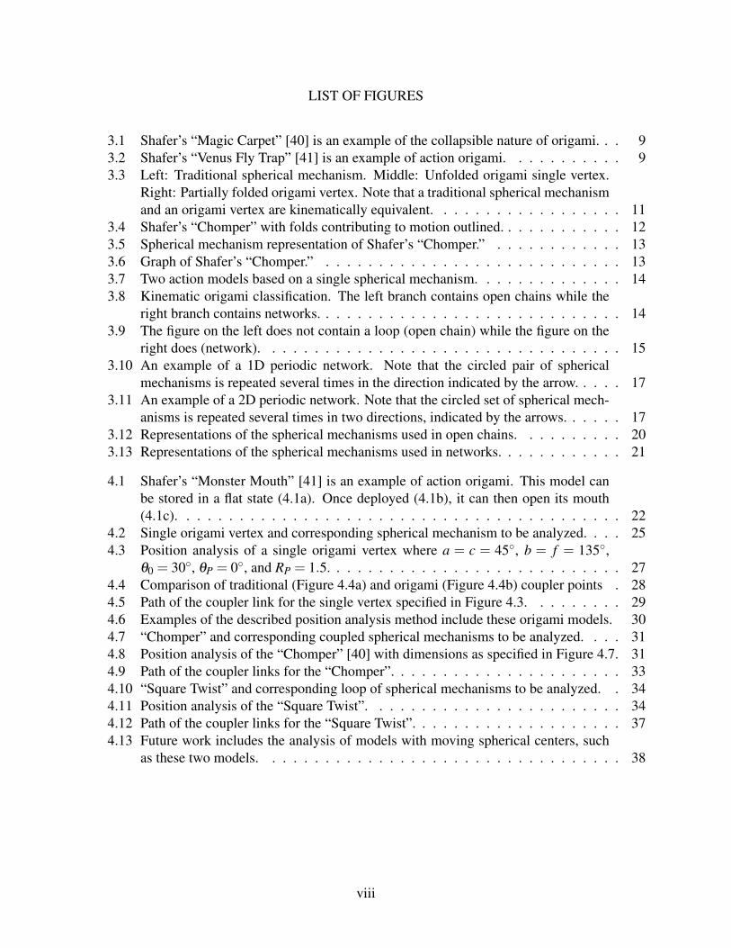
LIST OF TABLES . . . . . . . . . . . . . . . . . . . . . . . . . . . . . . . . . . . . . . . vi

LIST OF FIGURES . . . . . . . . . . . . . . . . . . . . . . . . . . . . . . . . . . . . . . vii

Chapter 1 Introduction . . . . . . . . . . . . . . . . . . . . . . . . . . . . . . . . . . . 11.1 Motivation . . . . . . . . . . . . . . . . . . . . . . . . . . . . . . . . . . . . . . . 11.2 Thesis Objective . . . . . . . . . . . . . . . . . . . . . . . . . . . . . . . . . . . 11.3 Thesis Outline . . . . . . . . . . . . . . . . . . . . . . . . . . . . . . . . . . . . . 1

Chapter 2 Literature Review . . . . . . . . . . . . . . . . . . . . . . . . . . . . . . . 32.1 Introduction . . . . . . . . . . . . . . . . . . . . . . . . . . . . . . . . . . . . . . 32.2 Origami Engineering . . . . . . . . . . . . . . . . . . . . . . . . . . . . . . . . . 32.3 Reconfigurable Structures/Self-folding . . . . . . . . . . . . . . . . . . . . . . . . 52.4 Rigid Origami . . . . . . . . . . . . . . . . . . . . . . . . . . . . . . . . . . . . . 52.5 Origami Kinematics . . . . . . . . . . . . . . . . . . . . . . . . . . . . . . . . . . 62.6 Alternate Materials . . . . . . . . . . . . . . . . . . . . . . . . . . . . . . . . . . 62.7 Origami Math . . . . . . . . . . . . . . . . . . . . . . . . . . . . . . . . . . . . . 72.8 Origami Diagrams . . . . . . . . . . . . . . . . . . . . . . . . . . . . . . . . . . 7

Chapter 3 A Classification of Action Origami as Systems of Spherical Mechanisms . 83.1 Introduction . . . . . . . . . . . . . . . . . . . . . . . . . . . . . . . . . . . . . . 83.2 Background . . . . . . . . . . . . . . . . . . . . . . . . . . . . . . . . . . . . . . 93.3 Approach . . . . . . . . . . . . . . . . . . . . . . . . . . . . . . . . . . . . . . . 113.4 Classification . . . . . . . . . . . . . . . . . . . . . . . . . . . . . . . . . . . . . 13

3.4.1 Single . . . . . . . . . . . . . . . . . . . . . . . . . . . . . . . . . . . . . 153.4.2 Coupled . . . . . . . . . . . . . . . . . . . . . . . . . . . . . . . . . . . . 153.4.3 N-long Linear Chain . . . . . . . . . . . . . . . . . . . . . . . . . . . . . 163.4.4 Tree . . . . . . . . . . . . . . . . . . . . . . . . . . . . . . . . . . . . . . 163.4.5 Single Loop . . . . . . . . . . . . . . . . . . . . . . . . . . . . . . . . . . 163.4.6 1D Periodic . . . . . . . . . . . . . . . . . . . . . . . . . . . . . . . . . . 163.4.7 2D Periodic . . . . . . . . . . . . . . . . . . . . . . . . . . . . . . . . . . 173.4.8 Non-periodic . . . . . . . . . . . . . . . . . . . . . . . . . . . . . . . . . 18

3.5 Classification Results . . . . . . . . . . . . . . . . . . . . . . . . . . . . . . . . . 183.6 Conclusion . . . . . . . . . . . . . . . . . . . . . . . . . . . . . . . . . . . . . . 18

Chapter 4 A Position Analysis of Coupled Spherical Mechanisms Found in ActionOrigami . . . . . . . . . . . . . . . . . . . . . . . . . . . . . . . . . . . . . 22

4.1 Introduction . . . . . . . . . . . . . . . . . . . . . . . . . . . . . . . . . . . . . . 224.2 Literature Review . . . . . . . . . . . . . . . . . . . . . . . . . . . . . . . . . . . 234.3 Method . . . . . . . . . . . . . . . . . . . . . . . . . . . . . . . . . . . . . . . . 24

4.3.1 Origami Vertex . . . . . . . . . . . . . . . . . . . . . . . . . . . . . . . . 254.3.2 Relationship Between Input and Output Angle . . . . . . . . . . . . . . . 25

v

4.3.3 Angle Between Input and Coupler . . . . . . . . . . . . . . . . . . . . . . 274.3.4 Equation for a Coupler Point . . . . . . . . . . . . . . . . . . . . . . . . . 27

4.4 Examples . . . . . . . . . . . . . . . . . . . . . . . . . . . . . . . . . . . . . . . 294.4.1 Coupled . . . . . . . . . . . . . . . . . . . . . . . . . . . . . . . . . . . . 304.4.2 Loop . . . . . . . . . . . . . . . . . . . . . . . . . . . . . . . . . . . . . 32

4.5 Future work . . . . . . . . . . . . . . . . . . . . . . . . . . . . . . . . . . . . . . 364.6 Conclusion . . . . . . . . . . . . . . . . . . . . . . . . . . . . . . . . . . . . . . 36

Chapter 5 Conclusion . . . . . . . . . . . . . . . . . . . . . . . . . . . . . . . . . . . 395.1 Conclusions . . . . . . . . . . . . . . . . . . . . . . . . . . . . . . . . . . . . . . 395.2 Future Work . . . . . . . . . . . . . . . . . . . . . . . . . . . . . . . . . . . . . . 39

REFERENCES . . . . . . . . . . . . . . . . . . . . . . . . . . . . . . . . . . . . . . . . . 41

Appendix A MATLAB Position Analysis Programs . . . . . . . . . . . . . . . . . . . . 45A.1 Required Functions . . . . . . . . . . . . . . . . . . . . . . . . . . . . . . . . . . 45

A.1.1 Spherical Four Bar (s4bar.m) . . . . . . . . . . . . . . . . . . . . . . . . . 45A.1.2 Plotting Formatter (plotformatter.m) . . . . . . . . . . . . . . . . . . . . . 46

A.2 Single . . . . . . . . . . . . . . . . . . . . . . . . . . . . . . . . . . . . . . . . . 47A.2.1 Single Coupler Path (SinglePath.m) . . . . . . . . . . . . . . . . . . . . . 47A.2.2 Single Coupler Motion (SingleMotion.m) . . . . . . . . . . . . . . . . . . 51

A.3 Chomper . . . . . . . . . . . . . . . . . . . . . . . . . . . . . . . . . . . . . . . 56A.3.1 Chomper Coupler Path (ChomperPath.m) . . . . . . . . . . . . . . . . . . 56A.3.2 Chomper Coupler Motion (ChomperMotion.m) . . . . . . . . . . . . . . . 60

A.4 Square Twist . . . . . . . . . . . . . . . . . . . . . . . . . . . . . . . . . . . . . 66A.4.1 Square Twist Coupler Path (SquarePath.m) . . . . . . . . . . . . . . . . . 66A.4.2 Square Twist Coupler Motion (SquareMotion.m) . . . . . . . . . . . . . . 71

vi

LIST OF TABLES

3.1 Classification of studied kinematic origami models . . . . . . . . . . . . . . . . . 18

vii

LIST OF FIGURES

3.1 Shafer’s “Magic Carpet” [40] is an example of the collapsible nature of origami. . . 93.2 Shafer’s “Venus Fly Trap” [41] is an example of action origami. . . . . . . . . . . 93.3 Left: Traditional spherical mechanism. Middle: Unfolded origami single vertex.

Right: Partially folded origami vertex. Note that a traditional spherical mechanismand an origami vertex are kinematically equivalent. . . . . . . . . . . . . . . . . . 11

3.4 Shafer’s “Chomper” with folds contributing to motion outlined. . . . . . . . . . . . 123.5 Spherical mechanism representation of Shafer’s “Chomper.” . . . . . . . . . . . . 133.6 Graph of Shafer’s “Chomper.” . . . . . . . . . . . . . . . . . . . . . . . . . . . . 133.7 Two action models based on a single spherical mechanism. . . . . . . . . . . . . . 143.8 Kinematic origami classification. The left branch contains open chains while the

right branch contains networks. . . . . . . . . . . . . . . . . . . . . . . . . . . . . 143.9 The figure on the left does not contain a loop (open chain) while the figure on the

right does (network). . . . . . . . . . . . . . . . . . . . . . . . . . . . . . . . . . 153.10 An example of a 1D periodic network. Note that the circled pair of spherical

mechanisms is repeated several times in the direction indicated by the arrow. . . . . 173.11 An example of a 2D periodic network. Note that the circled set of spherical mech-

anisms is repeated several times in two directions, indicated by the arrows. . . . . . 173.12 Representations of the spherical mechanisms used in open chains. . . . . . . . . . 203.13 Representations of the spherical mechanisms used in networks. . . . . . . . . . . . 21

4.1 Shafer’s “Monster Mouth” [41] is an example of action origami. This model canbe stored in a flat state (4.1a). Once deployed (4.1b), it can then open its mouth(4.1c). . . . . . . . . . . . . . . . . . . . . . . . . . . . . . . . . . . . . . . . . . 22

4.2 Single origami vertex and corresponding spherical mechanism to be analyzed. . . . 254.3 Position analysis of a single origami vertex where a = c = 45◦, b = f = 135◦,

θ0 = 30◦, θP = 0◦, and RP = 1.5. . . . . . . . . . . . . . . . . . . . . . . . . . . . 274.4 Comparison of traditional (Figure 4.4a) and origami (Figure 4.4b) coupler points . 284.5 Path of the coupler link for the single vertex specified in Figure 4.3. . . . . . . . . 294.6 Examples of the described position analysis method include these origami models. 304.7 “Chomper” and corresponding coupled spherical mechanisms to be analyzed. . . . 314.8 Position analysis of the “Chomper” [40] with dimensions as specified in Figure 4.7. 314.9 Path of the coupler links for the “Chomper”. . . . . . . . . . . . . . . . . . . . . . 334.10 “Square Twist” and corresponding loop of spherical mechanisms to be analyzed. . 344.11 Position analysis of the “Square Twist”. . . . . . . . . . . . . . . . . . . . . . . . 344.12 Path of the coupler links for the “Square Twist”. . . . . . . . . . . . . . . . . . . . 374.13 Future work includes the analysis of models with moving spherical centers, such

as these two models. . . . . . . . . . . . . . . . . . . . . . . . . . . . . . . . . . 38

viii

CHAPTER 1. INTRODUCTION

1.1 Motivation

Action origami represents an unexplored area of compact, deployable mechanisms with

motion in the deployed state. A better qualitative and quantitative understanding of action origami

could enable the application of action origami concepts in engineering applications. An under-

standing of what types of motion are possible in action origami is gained by classifying all possible

action origami models by their kinematic structure. Once these mechanism categories are deter-

mined, kinematic modeling of these groups will lead to analysis and synthesis, creating the ability

to design and optimize new mechanisms for use in deployable systems.

1.2 Thesis Objective

The purpose of this thesis is to lay the groundwork for the synthesis of compact, deployable

mechanisms and applications that also allow motion in the deployed state. This is performed by

investigating and classifying action origami models by their kinematic structure, followed by a

position analysis of several of the identified categories.

1.3 Thesis Outline

Chapter 1 introduces the topic by describing the motivation and purpose behind the re-

search.

As using origami as a design inspiration is a relatively new topic, a brief overview of

technical literature dealing with various aspects of origami and how it has been used in engineering

previously is presented in Chapter 2.

In Chapter 3, the structure of action origami that allows motion is found to be spherical

mechanisms. A new term, “kinematic origami”, is introduced to describe action origami models

1

which obtain motion through spherical mechanisms. Over 300 action origami models are classified

based on their spherical mechanism structure, resulting in 8 different categories. Portions of this

chapter will be published in the proceedings of the 2013 Design and Engineering Technical Con-

ferences (DETC), and the chapter has been accepted for publication in the Journal of Mechanical

Design.

Chapter 4 takes a deeper look at three of these categories, presenting a method for the

analysis of coupled systems of spherical mechanisms. Using existing spherical mechanism knowl-

edge, the path of coupler links for these categories is shown. This chapter is planned for future

submission.

Lastly, Chapter 5 includes conclusions drawn from the research as well as areas of future

work.

2

CHAPTER 2. LITERATURE REVIEW

2.1 Introduction

The amount of literature dealing with origami and its derivatives is very large and covers a

broad spectrum of disciplines. As a first step to viewing origami from an engineering perspective,

a thorough literature search was undertaken. Hundreds of articles were found relating to many dif-

ferent areas, from the mathematics behind origami principles to the application of these principles

to create unique designs. In order to deal with this abundance of literature, seven key topics were

identified under which the background research fell. These were:

• Origami Engineering

• Reconfigurable Structures

• Rigid Origami

• Origami Kinematics

• Alternate Materials

• Origami Math

• Origami Diagrams

Each of these areas will be discussed in more detail below.

2.2 Origami Engineering

As one long-term goal of this research is to discover new products or better ways to create

existing products, applications for which origami has already been used were important to find.

3

Many applications exist, and more are sure to come as a result of future research in the fields of

engineering and origami.

In general, origami has been looked to in design for, among other things, flat-foldability

(compactness) and aesthetic appeal. Many of the applications that were found dealt with storing

the product in a more compact state when not in use, and folding the product into its “use state”

when needed. Several applications of origami include:

• Sandwich cores for aircraft [1]

• Foldable composite beam [2]

• Packaging [3]

• Electro-chemical capacitors [4]

• Space telescope [5]

• Airbag folding [6]

• Solar sails [7]

• Backpacking/Picnic dishware [8]

• Foldable kayak [9]

• Stent [10]

• Automobile crash box [11]

• Architecture [12]

More information about origami in engineering can be found in a review article on the topic

written by Dureisseix [13].

4

2.3 Reconfigurable Structures/Self-folding

As a single piece of paper can yield an infinite number of designs, research has been di-

rected towards creating reconfigurable structures, or mechanisms that could fold themselves into

a variety of shapes depending on the given need. One group of researchers have investigated

programmable matter, or a material that can change its stiffness of shape at will [14]. They suc-

cessfully created a sheet of material that will fold itself into several shapes using shape-memory

alloy flexures.

A very interesting method for self-folding uses an ink jet printer to print an origami pattern

on a sheet of paper. As the ink dries, it causes the paper to fold into the shape that was printed [15].

Another novel method for self-folding involves using light with a specific polymer to in-

duce folding [16].

Investigation into universal crease patterns from which many shapes can be folded has also

been undertaken [17]. This is important as current technology somewhat restricts us to specify

crease lines beforehand.

Currently, work is being done on a multi-field responsive material that would fold itself

based on the application of an electric and/or magnetic field [18].

2.4 Rigid Origami

Rigid origami is a subset of origami that deals with treating panels as rigid. Many origami

models are rigid-foldable. Rigid-foldable models are easier to model and analyze than models

requiring flexible panels. Tomohiro Tachi, a major contributor in this area, has created a rigid

origami simulator which takes fold patterns created in a vector graphics program and visualizes

their folding [19]. Patterned cylinders have been investigated using rigid origami, which have

potential use in energy absorption [20].

Tachi has also created methods for the rigid-foldability of thick materials [21]. When

folding paper, its thickness can, most of the time, be discounted. When thickness is introduced,

however, many things taken for granted when folding paper must be addressed. This also has

application in using alternate materials in origami, as thickness is a consideration for most non-

paper materials.

5

Charles Hoberman, well-known for both his moving architecture and children’s toys, has a

patent dealing with the folding of structures made with thick hinged sheets [22].

2.5 Origami Kinematics

Obtaining a mathematical model for the motion of an origami model is an important first

step in the design of an origami-inspired product. While obtaining a desired motion by prototyping

is very possible, it can be time-consuming. Having a robust math model can allow the use of

kinematic tools for path, motion, and function generation as well as optimization. These tools

have the potential to both decrease time spent in design as well as increase performance.

Many papers have been written to describe the motion of origami as it folds. Jian Dai et

al. have written several articles describing the mobility and motions of carton folding using screw

theory and spherical kinematics [3, 23, 24]. The packaging/carton business is very large, but most

cartons are still assembled by hand. By obtaining a robust mathematical model, robots could be

programmed to fold these cartons [25].

Much of origami obtains its motion using spherical mechanisms. Spherical mechanisms

have been an area of research in mechanical engineering for a long time. C.H. Chiang uses spher-

ical trigonometry to create closed-form equations for the position, velocity, and acceleration of a

single spherical mechanism [26].

Origami motion has also been modeled using quaternions and dual quaternions [27], a

spring mass model [28], and affine transformations [29].

2.6 Alternate Materials

Paper is the material that has been used for origami since its beginnings. Paper is a remark-

ably unique material, creating a sharp crease when folded through the delamination of fibers [30].

Unfortunately, paper is not often a great engineering material.

There are several examples of alternate materials used in origami. Nano-patterned mem-

branes have been folded for 3D nanomanufacturing [31]. Origami structures have been 3D printed

and folded [4]. Industrial Origami, a design company specializing in origami designs, has patented

6

a pattern to cut into the desired crease site of thick steel sheets that allows them to be bent by

hand [32, 33].

2.7 Origami Math

Perhaps the largest quantity of origami research literature deals with origami math. There

are too many topics within origami math for this area to be described sufficiently in this review.

Two topics that are relevant to the work at hand are the determination of flat-foldability and algo-

rithmic design methods.

Determination of the flat-foldability of a single vertex is simple, but most origami models

and tesselations have many vertices. Global flat foldability, the case in which the entire model

composed of many vertices folds flat, is difficult to determine, though research is ongoing [34–36].

Robert Lang has a computational algorithm, known as Treemaker, which creates a crease

pattern based on a proportioned stick figure of the desired model [37]. This method could be of

assistance in the design of new products and mechanisms, expanding what is possible through the

use of computational software.

2.8 Origami Diagrams

Without origami diagrams many artists’ work would be unfoldable to origami enthusiasts.

There are many books on origami folding patterns. The books that were used for this research dealt

in particular with action origami. Two origami artists who do the most work in action origami

are Jeremy Shafer and Robert Lang. Their diagrams have been used most extensively in this

work [38–41].

7

CHAPTER 3. A CLASSIFICATION OF ACTION ORIGAMI AS SYSTEMS OF SPHER-ICAL MECHANISMS

3.1 Introduction

Origami, the Japanese art of folding paper, has been practiced for hundreds of years, inspir-

ing individuals with its beauty and complexity. The relatively recent application of mathematics to

origami has resulted in a large increase in both the number and sophistication of origami models.

From this growing repository of origami knowledge, solutions to engineering problems have been

discovered for applications as diverse as nanostructured 3D devices [4] and sandwich cores for

aircraft structures [1].

Many origami-based applications employ a collapsible mechanism that is compact while in

a stored state and deploys into a larger state. Thus, origami has provided insight into solutions that

are flat-foldable and collapsible (see Figure 3.1 for an example origami model). However, origami

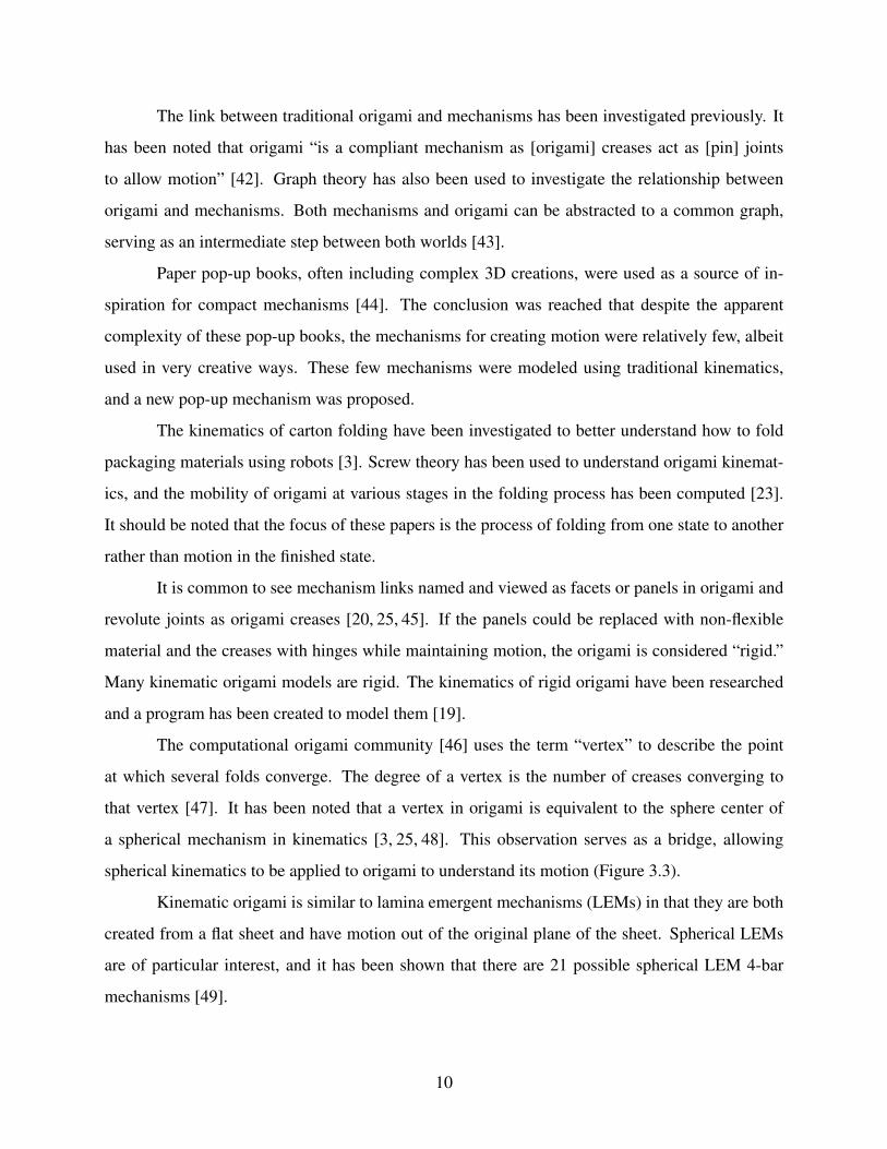
has not often been used to inspire products meant to move in their deployed state. Action origami

is a field of origami dealing with models that are folded so that they exhibit motion in their final,

deployed state (see Figure 3.2 for an example action origami model). Many action origami models

have been developed as children’s toys: flapping cranes, tops, and paper airplanes. There are in

fact hundreds of action origami models, many of which use complicated kinematics to achieve

motion in their deployed state. These motions are achieved from a single flat sheet of paper with

one manufacturing process — folding.

The field of action origami is a promising area for engineering solutions that has heretofore

been largely unexplored. The motions found in action origami have the potential to provide solu-

tions for the design of mechanisms that need to be stored in a compact state. A better understanding

of the mechanisms used to create motion in action origami could be a foundation for developing a

new source of concepts for deployable, movable engineering solutions.

8

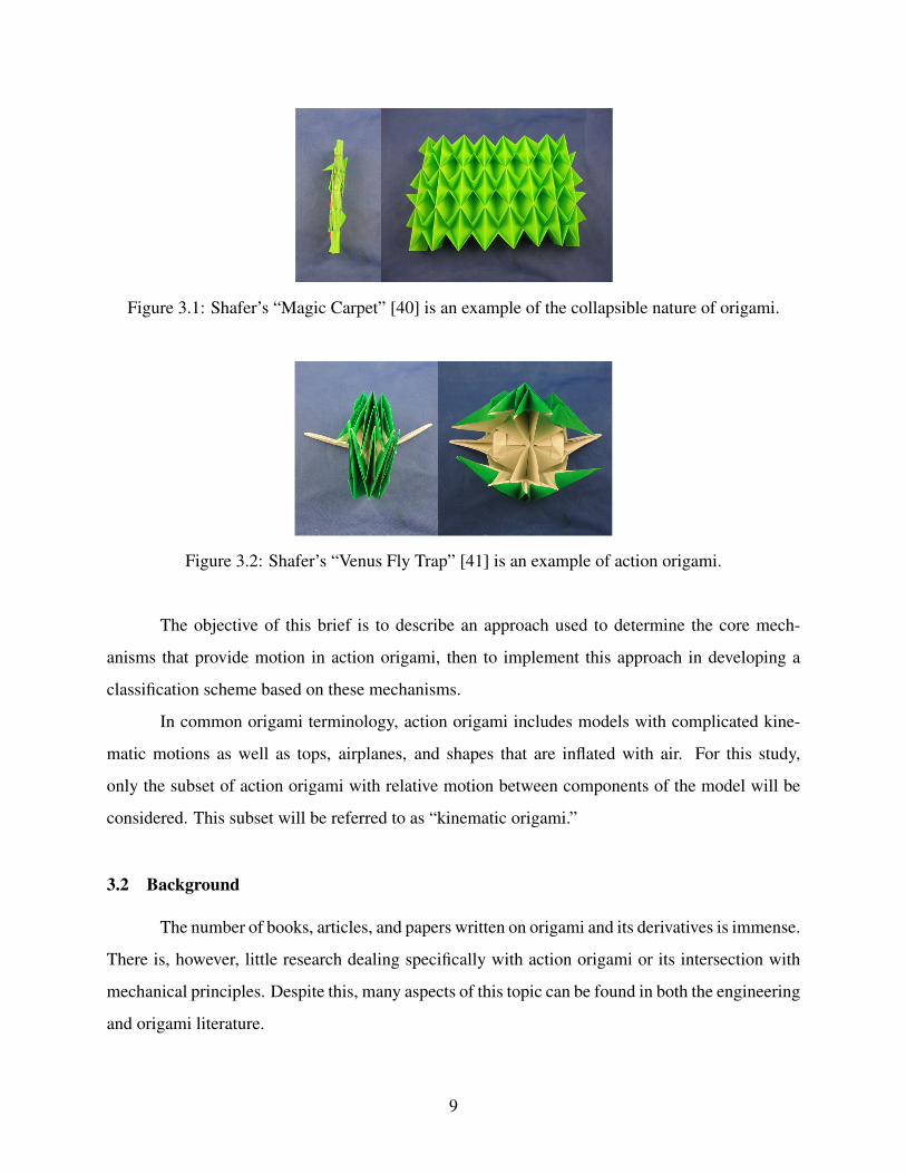
Figure 3.1: Shafer’s “Magic Carpet” [40] is an example of the collapsible nature of origami.

Figure 3.2: Shafer’s “Venus Fly Trap” [41] is an example of action origami.

The objective of this brief is to describe an approach used to determine the core mech-

anisms that provide motion in action origami, then to implement this approach in developing a

classification scheme based on these mechanisms.

In common origami terminology, action origami includes models with complicated kine-

matic motions as well as tops, airplanes, and shapes that are inflated with air. For this study,

only the subset of action origami with relative motion between components of the model will be

considered. This subset will be referred to as “kinematic origami.”

3.2 Background

The number of books, articles, and papers written on origami and its derivatives is immense.

There is, however, little research dealing specifically with action origami or its intersection with

mechanical principles. Despite this, many aspects of this topic can be found in both the engineering

and origami literature.

9

The link between traditional origami and mechanisms has been investigated previously. It

has been noted that origami “is a compliant mechanism as [origami] creases act as [pin] joints

to allow motion” [42]. Graph theory has also been used to investigate the relationship between

origami and mechanisms. Both mechanisms and origami can be abstracted to a common graph,

serving as an intermediate step between both worlds [43].

Paper pop-up books, often including complex 3D creations, were used as a source of in-

spiration for compact mechanisms [44]. The conclusion was reached that despite the apparent

complexity of these pop-up books, the mechanisms for creating motion were relatively few, albeit

used in very creative ways. These few mechanisms were modeled using traditional kinematics,

and a new pop-up mechanism was proposed.

The kinematics of carton folding have been investigated to better understand how to fold

packaging materials using robots [3]. Screw theory has been used to understand origami kinemat-

ics, and the mobility of origami at various stages in the folding process has been computed [23].

It should be noted that the focus of these papers is the process of folding from one state to another

rather than motion in the finished state.

It is common to see mechanism links named and viewed as facets or panels in origami and

revolute joints as origami creases [20, 25, 45]. If the panels could be replaced with non-flexible

material and the creases with hinges while maintaining motion, the origami is considered “rigid.”

Many kinematic origami models are rigid. The kinematics of rigid origami have been researched

and a program has been created to model them [19].

The computational origami community [46] uses the term “vertex” to describe the point

at which several folds converge. The degree of a vertex is the number of creases converging to

that vertex [47]. It has been noted that a vertex in origami is equivalent to the sphere center of

a spherical mechanism in kinematics [3, 25, 48]. This observation serves as a bridge, allowing

spherical kinematics to be applied to origami to understand its motion (Figure 3.3).

Kinematic origami is similar to lamina emergent mechanisms (LEMs) in that they are both

created from a flat sheet and have motion out of the original plane of the sheet. Spherical LEMs

are of particular interest, and it has been shown that there are 21 possible spherical LEM 4-bar

mechanisms [49].

10

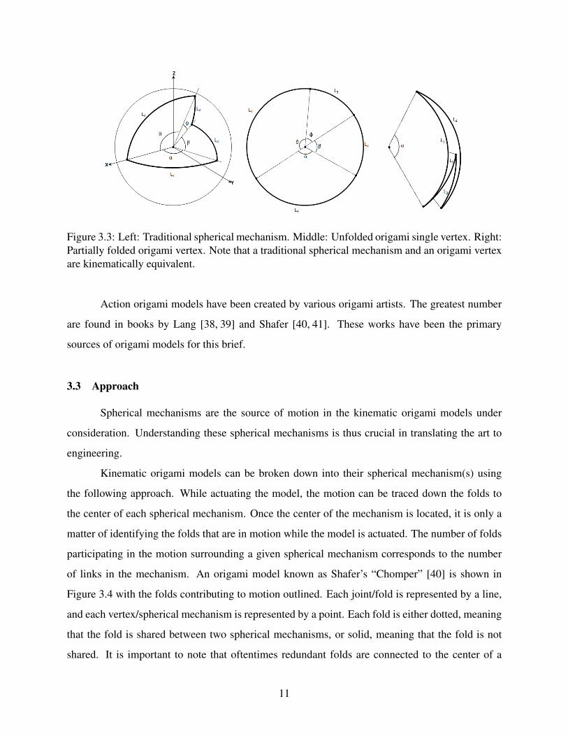
Figure 3.3: Left: Traditional spherical mechanism. Middle: Unfolded origami single vertex. Right:Partially folded origami vertex. Note that a traditional spherical mechanism and an origami vertexare kinematically equivalent.

Action origami models have been created by various origami artists. The greatest number

are found in books by Lang [38, 39] and Shafer [40, 41]. These works have been the primary

sources of origami models for this brief.

3.3 Approach

Spherical mechanisms are the source of motion in the kinematic origami models under

consideration. Understanding these spherical mechanisms is thus crucial in translating the art to

engineering.

Kinematic origami models can be broken down into their spherical mechanism(s) using

the following approach. While actuating the model, the motion can be traced down the folds to

the center of each spherical mechanism. Once the center of the mechanism is located, it is only a

matter of identifying the folds that are in motion while the model is actuated. The number of folds

participating in the motion surrounding a given spherical mechanism corresponds to the number

of links in the mechanism. An origami model known as Shafer’s “Chomper” [40] is shown in

Figure 3.4 with the folds contributing to motion outlined. Each joint/fold is represented by a line,

and each vertex/spherical mechanism is represented by a point. Each fold is either dotted, meaning

that the fold is shared between two spherical mechanisms, or solid, meaning that the fold is not

shared. It is important to note that oftentimes redundant folds are connected to the center of a

11

Figure 3.4: Shafer’s “Chomper” with folds contributing to motion outlined.

spherical mechanism. These folds may be present due to intermediate folds that were used to

achieve the desired final geometry but do not contribute to the model’s motion.

While the above approach can be effective in determining both the number of mechanisms

and their degrees, artistic features of the origami model (fangs, flippers, ears, etc.) often disguise

the mechanisms. To illustrate a model’s spherical mechanisms more clearly, each mechanism can

be folded from a sheet of circular origami paper and attached as they would be in the origami

model. Representations of these circular paper models were then modeled using Solidworks, as

seen in Figure 3.5. Two colors were used for clarity in the figures. Using this approach, it was

easier to identify the fundamental mechanisms producing motion in each model. This also allowed

for models to be grouped based on similar fundamental mechanism structures.

Graphs were also employed to abstract the origami models further, removing all details

except for the number of mechanisms and the connections between them. This was helpful in

generalizing the origami to the point that it could be easily classified. An example of such a

representation is seen in Figure 3.6.

This approach was used to analyze approximately 300 action origami models available in

the origami literature. Each model displaying relative motion (about 140 models) was folded and

studied. Not every model could be included, as the field of action origami is continually growing.

The results of this analysis of existing action origami models were used to develop the clas-

sification scheme described below. Note that the specifics of each spherical mechanism (number

of links, link lengths, link shapes, internal angles) are not mentioned in this classification scheme.

It is meant to be as general as possible, presenting the idea that most action origami models share a

few common configurations of mechanisms. The flexibility to change link length, number of links,

and link shape is what allows the same mechanisms to provide the motion for very different mod-

12

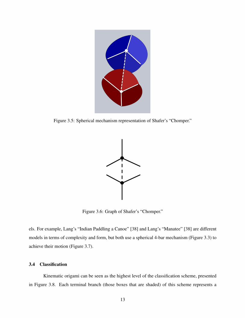
Figure 3.5: Spherical mechanism representation of Shafer’s “Chomper.”

Figure 3.6: Graph of Shafer’s “Chomper.”

els. For example, Lang’s “Indian Paddling a Canoe” [38] and Lang’s “Manatee” [38] are different

models in terms of complexity and form, but both use a spherical 4-bar mechanism (Figure 3.3) to

achieve their motion (Figure 3.7).

3.4 Classification

Kinematic origami can be seen as the highest level of the classification scheme, presented

in Figure 3.8. Each terminal branch (those boxes that are shaded) of this scheme represents a

13

Figure 3.7: Two action models based on a single spherical mechanism.

Figure 3.8: Kinematic origami classification. The left branch contains open chains while the rightbranch contains networks.

category under which a group of kinematic origami models fall. Each of these categories will be

briefly discussed below.

While many kinematic origami models have complex and diverse motion, once they are

viewed in the light of vertices and spherical mechanisms, the models are based on a few funda-

mental mechanisms. When the artistic elements are stripped away, most kinematic origami can be

reduced to one, two, or a system of interconnected spherical mechanisms. When this analysis is

conducted it is apparent that a relatively small number of spherical mechanism combinations can

produce a wide range of interesting motion with artistic variations in composition.

Note that figures displaying each category name, a representative model with outlined

folds, the 3D model representation, and the graph representation are shown in Figure 3.12 and

14

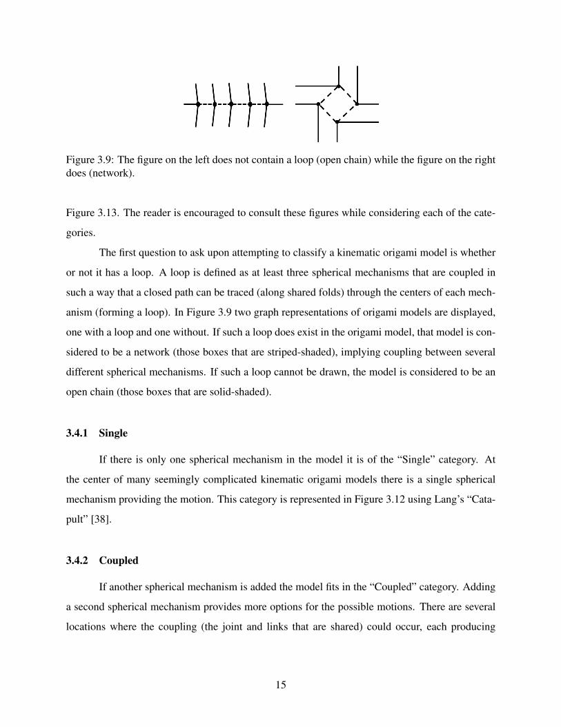
Figure 3.9: The figure on the left does not contain a loop (open chain) while the figure on the rightdoes (network).

Figure 3.13. The reader is encouraged to consult these figures while considering each of the cate-

gories.

The first question to ask upon attempting to classify a kinematic origami model is whether

or not it has a loop. A loop is defined as at least three spherical mechanisms that are coupled in

such a way that a closed path can be traced (along shared folds) through the centers of each mech-

anism (forming a loop). In Figure 3.9 two graph representations of origami models are displayed,

one with a loop and one without. If such a loop does exist in the origami model, that model is con-

sidered to be a network (those boxes that are striped-shaded), implying coupling between several

different spherical mechanisms. If such a loop cannot be drawn, the model is considered to be an

open chain (those boxes that are solid-shaded).

3.4.1 Single

If there is only one spherical mechanism in the model it is of the “Single” category. At

the center of many seemingly complicated kinematic origami models there is a single spherical

mechanism providing the motion. This category is represented in Figure 3.12 using Lang’s “Cata-

pult” [38].

3.4.2 Coupled

If another spherical mechanism is added the model fits in the “Coupled” category. Adding

a second spherical mechanism provides more options for the possible motions. There are several

locations where the coupling (the joint and links that are shared) could occur, each producing

15

unique motion. Coupling of two spherical mechanisms is often used to create mouths for origami

creations. An example of this category is farelly’s “Flapping Butterfly” [38], seen in Figure 3.12.

3.4.3 N-long Linear Chain

If there are more than two spherical mechanisms coupled with no loops, the model belongs

to the category “N-long Linear Chain.” As the category title suggests, any number of mechanisms

can be coupled to one another, as long as they remain linear. An example of this is Shafer’s “Frog’s

Tongue” [41] (Figure 3.12). It is allowed for the orientation of each mechanism to be different, so

long as the beginning and ending mechanisms share only one joint while all others share only two.

3.4.4 Tree

The last category that is an open chain is the “Tree.” This category allows additional joints

to be shared from the mechanisms in a chain. No kinematic origami models were found that

belonged to this category, although it is clear that this category can exist. A modified version of

Shafer’s “Frog’s Tongue” [41], as shown in Figure 3.12, was designed and folded to provide an

example of an origami “Tree.” The absence of models in this area suggests a new area for origami

artists to apply their creativity.

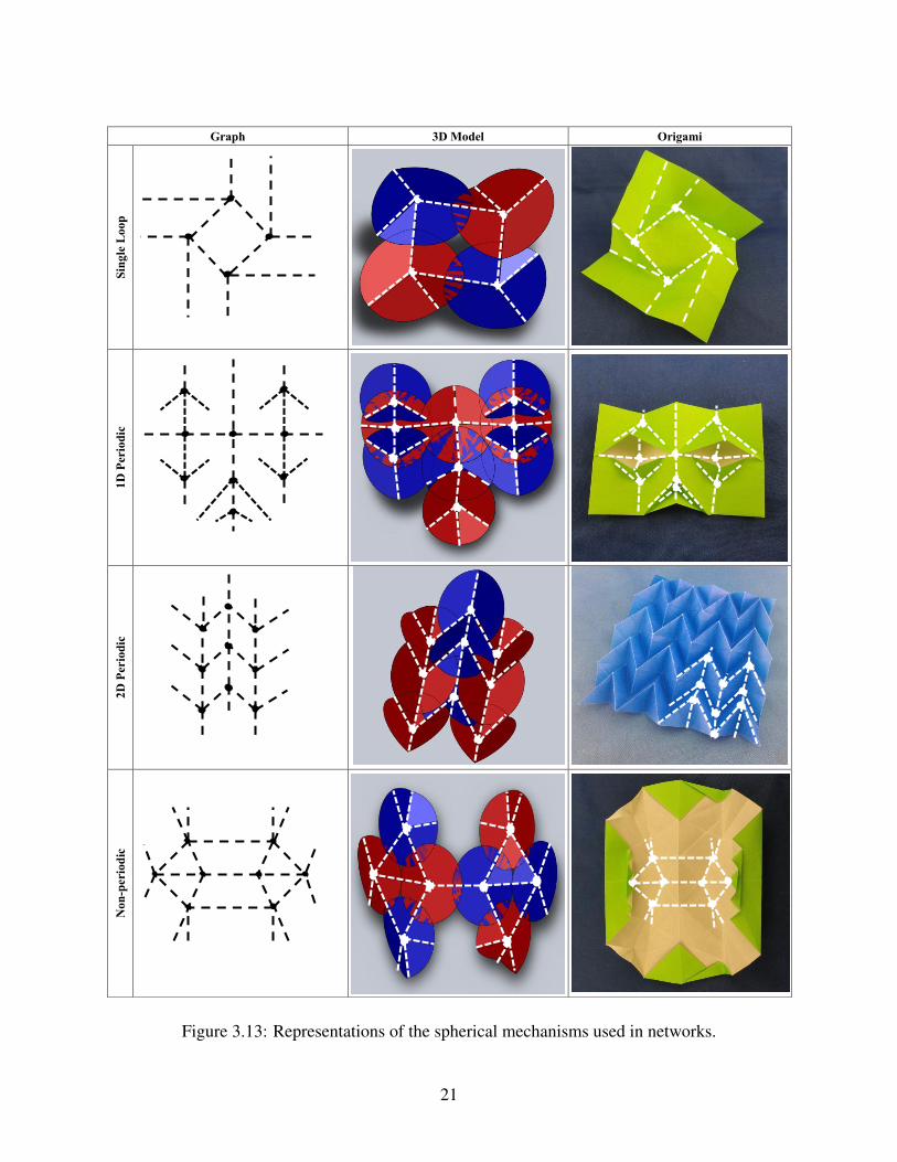
3.4.5 Single Loop

If there is only one loop in the model it is of the class “Single Loop.” An example mech-

anism is the traditional “Square Twist,” shown in Figure 3.13. Note that it is not important how

many unshared joints there are, only that a loop can be formed from the shared joints.

3.4.6 1D Periodic

If the model contains multiple loops, it must be determined if the network is “1D Periodic.”

The determination of multiple loops includes loops that share connections with other loops (they

do not have to be completely unique). For a set of spherical mechanisms with multiple loops to be

1D periodic, a subset of these mechanisms must be translated along one direction, i.e. the model

16

Figure 3.10: An example of a 1D periodic network. Note that the circled pair of spherical mecha-nisms is repeated several times in the direction indicated by the arrow.

Figure 3.11: An example of a 2D periodic network. Note that the circled set of spherical mecha-nisms is repeated several times in two directions, indicated by the arrows.

consists of two or more identical pieces connected along a line (Figure 3.10). Shafer’s “Blinking

Eyes” [41], seen in Figure 3.13, is essentially a 1D periodic network.

3.4.7 2D Periodic

If the model is periodic in an additional direction (Figure 3.11) it is “2D Periodic.” Many

of the action tessellations that were studied are included in this 2D periodic class. An example of

a 2D periodic network is Miura’s “Miura-Ori Pattern” (Figure 3.13), which has been used in map

and space solar array folding [50].

17

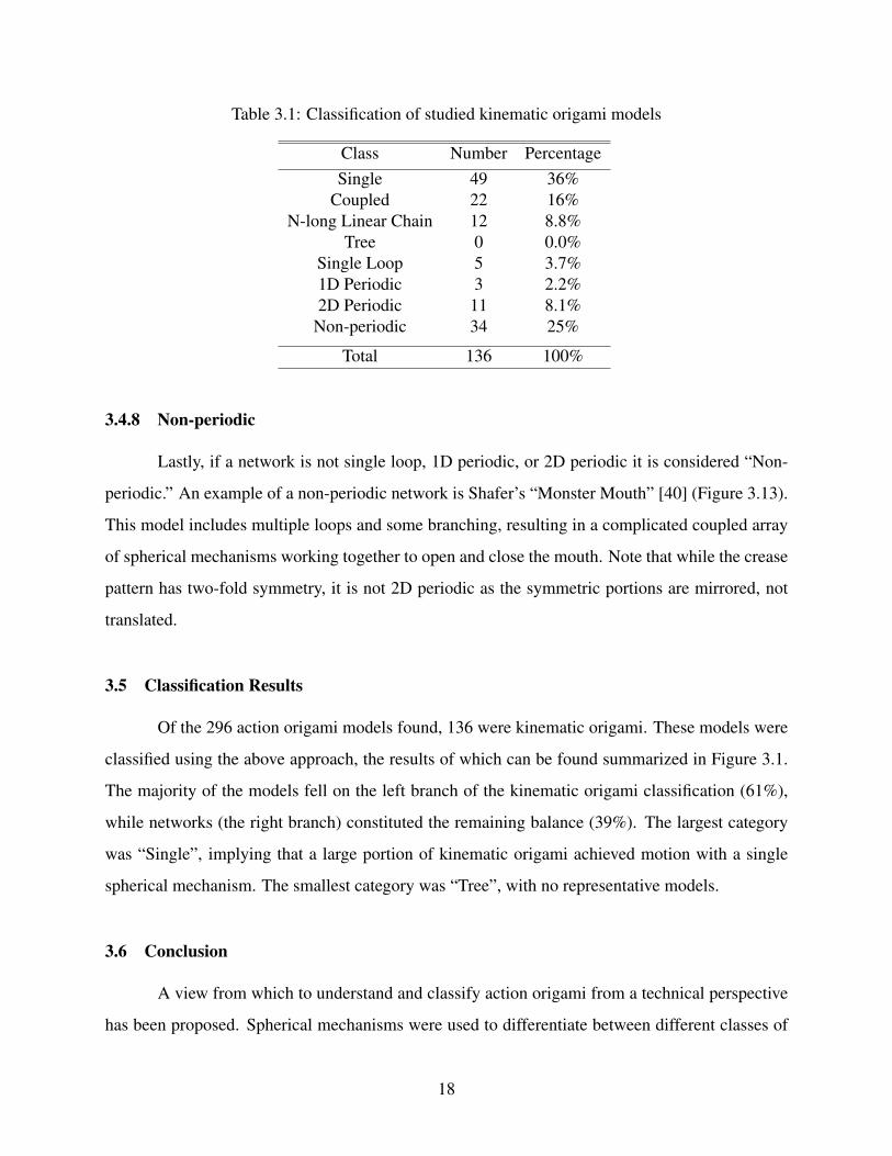
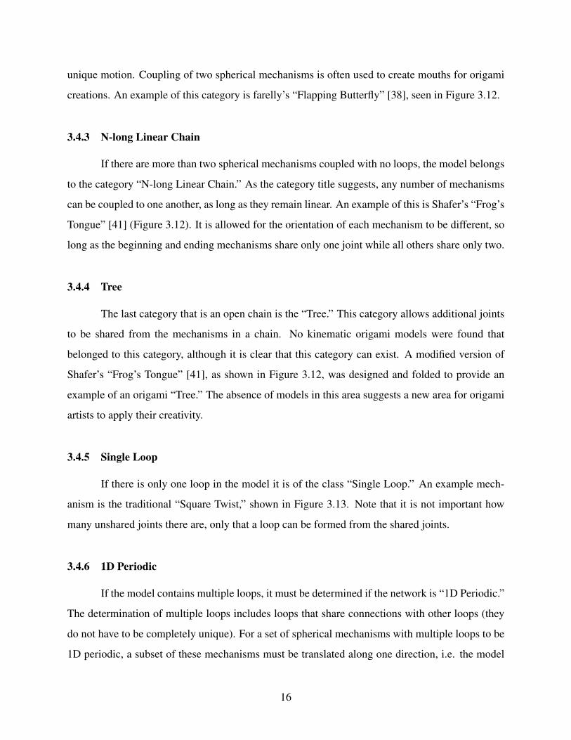
Table 3.1: Classification of studied kinematic origami models

Class Number PercentageSingle 49 36%

Coupled 22 16%N-long Linear Chain 12 8.8%

Tree 0 0.0%Single Loop 5 3.7%1D Periodic 3 2.2%2D Periodic 11 8.1%

Non-periodic 34 25%

Total 136 100%

3.4.8 Non-periodic

Lastly, if a network is not single loop, 1D periodic, or 2D periodic it is considered “Non-

periodic.” An example of a non-periodic network is Shafer’s “Monster Mouth” [40] (Figure 3.13).

This model includes multiple loops and some branching, resulting in a complicated coupled array

of spherical mechanisms working together to open and close the mouth. Note that while the crease

pattern has two-fold symmetry, it is not 2D periodic as the symmetric portions are mirrored, not

translated.

3.5 Classification Results

Of the 296 action origami models found, 136 were kinematic origami. These models were

classified using the above approach, the results of which can be found summarized in Figure 3.1.

The majority of the models fell on the left branch of the kinematic origami classification (61%),

while networks (the right branch) constituted the remaining balance (39%). The largest category

was “Single”, implying that a large portion of kinematic origami achieved motion with a single

spherical mechanism. The smallest category was “Tree”, with no representative models.

3.6 Conclusion

A view from which to understand and classify action origami from a technical perspective

has been proposed. Spherical mechanisms were used to differentiate between different classes of

18

kinematic origami. It is anticipated that the identification of these classes will serve as the founda-

tion for creating unique mechanisms to be used in engineering applications that take advantage of

the characteristics of origami, namely deployability and extreme compactness. In addition, kine-

matic origami-based mechanisms are not only compact when stored and deployable, they have

motion in the deployed state that can be critical for function. Lastly, a category of kinematic

origami has been identified that contains few models, signifying an area for action origami artists

to further apply their creativity.

19

Graph 3D Model Origami Si

ngle

Cou

pled

N-L

ong

Line

ar C

hain

Tre

e

Figure 3.12: Representations of the spherical mechanisms used in open chains.

20

Graph 3D Model Origami Si

ngle

Loo

p

1D P

erio

dic

2D P

erio

dic

Non

-per

iodi

c

Figure 3.13: Representations of the spherical mechanisms used in networks.

21

CHAPTER 4. A POSITION ANALYSIS OF COUPLED SPHERICAL MECHANISMSFOUND IN ACTION ORIGAMI

4.1 Introduction

The ancient Japanese art of origami has intrigued people for centuries with a beautiful

complexity arising from the single fabrication process of folding. The quantity and complexity

of origami models has been increasing partly due to the introduction of mathematical tools which

model and characterize the design parameters found in the art [19, 37]. Engineers and designers

have looked to origami for inspiration due to its potential in deployable systems. Origami, for

example, has been used as a source of inspiration for space applications [5] and automobile safety

[6, 11].

(a) (b) (c)

Figure 4.1: Shafer’s “Monster Mouth” [41] is an example of action origami. This model can bestored in a flat state (4.1a). Once deployed (4.1b), it can then open its mouth (4.1c).

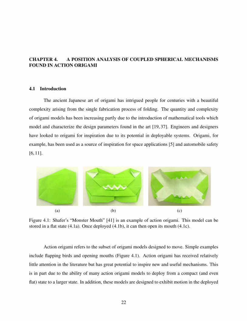
Action origami refers to the subset of origami models designed to move. Simple examples

include flapping birds and opening mouths (Figure 4.1). Action origami has received relatively

little attention in the literature but has great potential to inspire new and useful mechanisms. This

is in part due to the ability of many action origami models to deploy from a compact (and even

flat) state to a larger state. In addition, these models are designed to exhibit motion in the deployed

22

state. There are several areas of application for such mechanisms, including solar pointing arrays

and minimally invasive surgical tools.

Action origami has been shown to achieve motion through the use of spherical mecha-

nisms [25]. Action origami that achieves motion through the use of spherical mechanisms is termed

“kinematic origami.” All possible kinematic origami configurations have been classified based on

the number and arrangement of spherical mechanisms [51]. Some kinematic origami models con-

tain dozens of coupled spherical mechanisms, but can be fabricated by simple folding in just a few

minutes. As kinematic origami often utilizes symmetry for visual appeal, many models consist-

ing of several spherical mechanisms use the same mechanism (equivalent link lengths) repeated

throughout the model.

In order to utilize the unique properties of kinematic origami in engineering design, the

kinematics of coupled spherical mechanism systems must first be understood. The current liter-

ature dealing with coupled spherical systems is sparse, possibly because there has not previously

been motivation to investigate them. Recent studies show that spherical mechanisms (both single

and coupled) demonstrate several advantages over planar mechanisms including lower values of

inertial forces and better pressure angle values [52, 53].

Making explicit the commonality between spherical mechanisms and kinematic origami

makes possible mathematical models that can greatly enhance the analysis, optimization, and syn-

thesis of new mechanisms with motion inspired by kinematic origami.

The purpose of this paper is to take a first step toward the advanced analysis and synthesis

of kinematic origami-inspired mechanisms by describing and demonstrating a method for the po-

sition analysis of coupled systems of repeated spherical mechanisms. Such repeated systems are

common in kinematic origami models and tessellations. This method has the potential to make

kinematic origami-based design more effective and structured, moving much of the design process

to computer-based tools.

4.2 Literature Review

The growing relationship between origami artists and technical designers has resulted in

increased literature on the subject of connections between origami and mechanism design. Green-

berg et al. [54] point out that origami is a form of compliant mechanisms where the creases act as

23

pin joints to allow movement, and goes on to show that graph theory can act as a step between kine-

matics and origami. Liu and Dai similarly identify carton panels as mechanism links and creases

as joints when investigating carton mobility [23].

The origami community has long identified and labeled characteristics of origami models

and has particularly noted movement about a single vertex [20], the point at which fold lines

converge. It has been noted that an origami vertex (including the surrounding folds and panels) is

equivalent to a traditional spherical mechanism [3, 25, 48].

A recent examination of action origami models verifies that much of action origami is

composed of configurations of spherical mechanisms [51], where action origami which achieves

motion from spherical mechanisms is called “kinematic origami”. A classification scheme based

on the spherical mechanism structure of kinematic origami was presented that encompasses all

possible configurations. Several of these categories, “Single”, “Coupled”, and “Loop”, are investi-

gated in this paper.

Lamina emergent mechanisms (LEMs) are a subset of compliant mechanisms that are

monolithic, planar, and have motion emerging from the plane of fabrication [55]. Action origami

shares all of these characteristics. All possible LEM spherical mechanisms have been classi-

fied [49], resulting in 21 possible LEM spherical 4R types being sorted into 3 categories.

The motion of origami has been investigated previously using several different methods.

Screw theory has been used to calculate the mobility of a carton during the folding process [23].

Spherical trigonometry has been utilized to perform some motion studies of a packaging carton

[56]. Quaternions and dual quaternions have been used to analyze the motion of an origami model

known as the square twist [27]. Other methods have also been used [19, 28, 29].

The motion of traditional spherical mechanisms is well-documented [26, 57, 58], and the

modeling and visualization of spherical mechanisms has been demonstrated [59].

4.3 Method

This section describes the position analysis of a single origami vertex, which is the basic

building block of the more complex systems described later. Many multi-vertex kinematic origami

models are composed of the same mechanism repeated one or more times, thus the results of one

vertex can be translated and rotated to the other vertices. This is demonstrated with two examples:

24

Shafer’s “Chomper” [40] and the traditional “Square Twist”. Taking advantage of symmetry in this

manner can result in a significant reduction of computation time for larger multi-vertex models.

4.3.1 Origami Vertex

As mentioned above, an origami vertex is equivalent to a spherical mechanism when folds

are treated as joints and panels as links. A byproduct of the flat-foldability of origami is the fact

that all origami vertices’ link lengths sum to 360◦. This means that each origami vertex is actually

a spherical change point mechanism. Traditional spherical mechanisms reside on a portion of

a sphere (less than a hemisphere) whereas an origami vertex resides on an entire hemisphere.

Although other types are possible, the majority of vertices found in action origami have 4 links,

and thus only spherical 4R mechanisms are discussed below.

(a) Single origami vertex. Note that a+c+b+ f = 360◦.

(b) Equivalent spherical mechanism withimportant angles specified.

Figure 4.2: Single origami vertex and corresponding spherical mechanism to be analyzed.

4.3.2 Relationship Between Input and Output Angle

Let us consider the origami vertex shown in Figure 4.2a and its corresponding spherical

mechanism in Figure 4.2b. Note that we decide upon a link that will be grounded. Also, a radius

25

is selected for the mechanism because this will determine joint locations along the folds. We will

use a radius of 1, or the unit sphere. The input angle, φ , is defined as the internal angle between

ground and the input link. The output angle, ψ , is defined as the external angle between ground

and the output link.

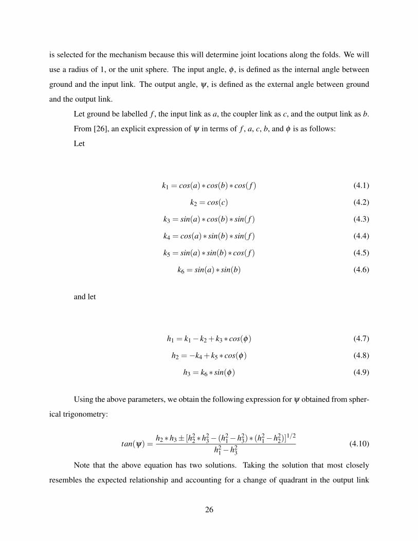
Let ground be labelled f , the input link as a, the coupler link as c, and the output link as b.

From [26], an explicit expression of ψ in terms of f , a, c, b, and φ is as follows:

Let

k1 = cos(a)∗ cos(b)∗ cos( f ) (4.1)

k2 = cos(c) (4.2)

k3 = sin(a)∗ cos(b)∗ sin( f ) (4.3)

k4 = cos(a)∗ sin(b)∗ sin( f ) (4.4)

k5 = sin(a)∗ sin(b)∗ cos( f ) (4.5)

k6 = sin(a)∗ sin(b) (4.6)

and let

h1 = k1 − k2 + k3 ∗ cos(φ) (4.7)

h2 =−k4 + k5 ∗ cos(φ) (4.8)

h3 = k6 ∗ sin(φ) (4.9)

Using the above parameters, we obtain the following expression for ψ obtained from spher-

ical trigonometry:

tan(ψ) =h2 ∗h3 ± [h2

2 ∗h23 − (h2

1 −h23)∗ (h2

1 −h22)]

1/2

h21 −h2

3(4.10)

Note that the above equation has two solutions. Taking the solution that most closely

resembles the expected relationship and accounting for a change of quadrant in the output link

26

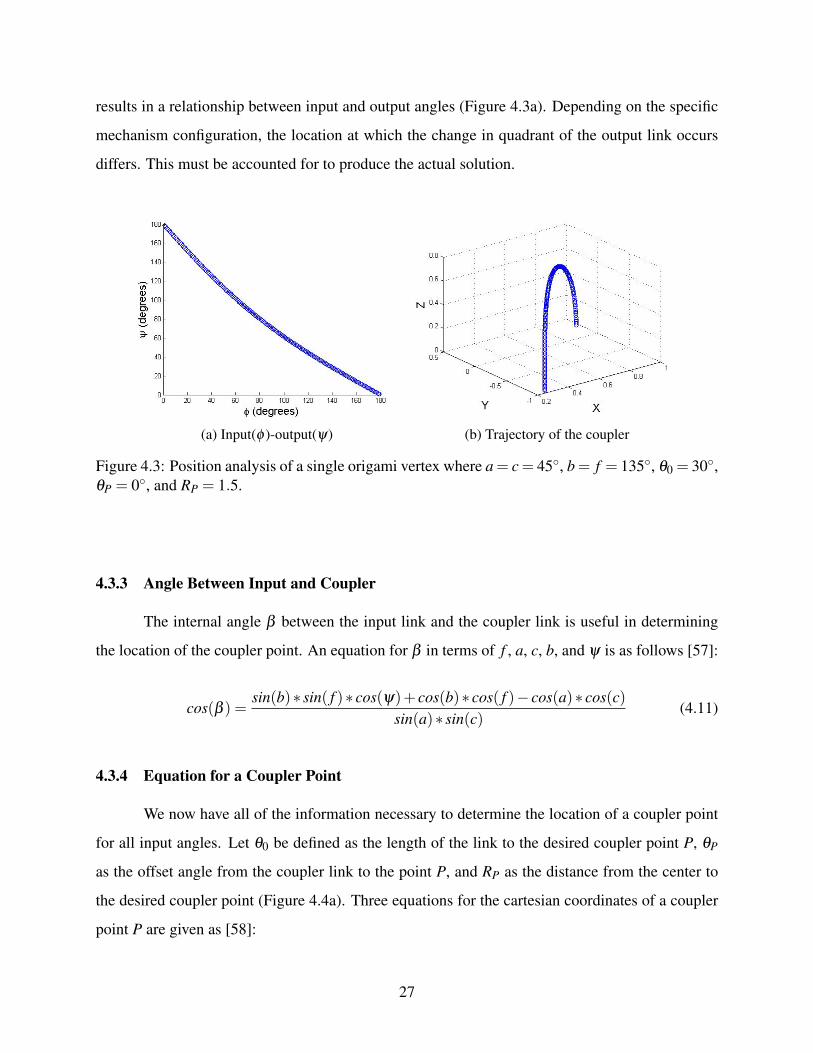
results in a relationship between input and output angles (Figure 4.3a). Depending on the specific

mechanism configuration, the location at which the change in quadrant of the output link occurs

differs. This must be accounted for to produce the actual solution.

(a) Input(φ )-output(ψ) (b) Trajectory of the coupler

Figure 4.3: Position analysis of a single origami vertex where a= c= 45◦, b= f = 135◦, θ0 = 30◦,θP = 0◦, and RP = 1.5.

4.3.3 Angle Between Input and Coupler

The internal angle β between the input link and the coupler link is useful in determining

the location of the coupler point. An equation for β in terms of f , a, c, b, and ψ is as follows [57]:

cos(β ) =sin(b)∗ sin( f )∗ cos(ψ)+ cos(b)∗ cos( f )− cos(a)∗ cos(c)

sin(a)∗ sin(c)(4.11)

4.3.4 Equation for a Coupler Point

We now have all of the information necessary to determine the location of a coupler point

for all input angles. Let θ0 be defined as the length of the link to the desired coupler point P, θP

as the offset angle from the coupler link to the point P, and RP as the distance from the center to

the desired coupler point (Figure 4.4a). Three equations for the cartesian coordinates of a coupler

point P are given as [58]:

27

rPx = [cos(θ0)∗ cos(a)+ sin(θ0)∗ cos(β +θP)∗ sin(a)]∗RP (4.12)

(4.13)rPy = [cos(θ0) ∗ cos(φ) ∗ sin(a) + sin(θ0) ∗ sin(φ) ∗ sin(β + θP)−sin(θ0) ∗ cos(β + θP) ∗ cos(a) ∗ cos(φ)] ∗ RP

(4.14)rPz = [cos(θ0) ∗ sin(φ) ∗ sin(a)− sin(θ0) ∗ cos(φ) ∗ sin(β + θP)−sin(θ0) ∗ cos(β + θP) ∗ cos(a) ∗ sin(φ)] ∗ RP

(a) Traditional coupler point (b) Origami vertex coupler point

Figure 4.4: Comparison of traditional (Figure 4.4a) and origami (Figure 4.4b) coupler points

Note that θP causes the coupler point to rest on the sphere at radius RP. As origami deals

with flat panels for links rather than the traditional spherical links, a coupler point for origami

can be defined with θ0 as described above, θP = 0, and a radius RP to the desired coupler point

(Figure 4.4b).

The path of the coupler point as a function of the input angle is shown in Figure 4.3b and

the path of the coupler link for several input angles is shown in Figure 4.5.

28

(a) φ = 1◦ (b) φ = 60◦

(c) φ = 120◦ (d) φ = 179◦

Figure 4.5: Path of the coupler link for the single vertex specified in Figure 4.3.

4.4 Examples

With the equations for the basic building block defined, it is possible to extend the model

to systems with multiple vertices. This section two examples of the position analysis of coupled

spherical systems. The first is Shafer’s “Chomper”, which is composed of two identical spherical

mechanisms coupled to one another (Figure 4.6a). This configuration is commonly used in action

origami as a mouth for various creatures.

The second example is a model known as the “Square Twist” in which 4 identical spherical

mechanisms are coupled to one another in a loop (Figure 4.6b).

29

(a) Shafer’s “Chomper” model [40]. (b) “Square Twist” model.

Figure 4.6: Examples of the described position analysis method include these origami models.

It should be pointed out that in both examples the spherical centers (two in the first example

and four in the second) are fixed to ground. This simplifies the analysis, allowing the angles and

coupler position of one spherical mechanism to be solved for all input angles, the results of which

are simply translated and rotated to the other spherical centers (as they are identical) to understand

the bulk motion of the mechanism.

4.4.1 Coupled

The “Chomper” model is composed of two identical spherical mechanisms which are cou-

pled as shown in Figure 4.7a. A more traditional representation the spherical mechanism located

at the origin is shown in Figure 4.7b. By analyzing one mechanism and applying the results to the

other mechanism the motion of the entire model can be discovered in an efficient manner. Note

that the second mechanism is translated 1 unit (as we are using the unit sphere) in the x-direction

and rotated 180 degrees from the first mechanism.

Solving the first spherical mechanism yields the input(φ )-output(ψ) relationship found in

Figure 4.8a. Again, the input-output relationship of the second mechanism is similar to that of the

first. The approach for translating the coupler curve from the first mechanism to the second and

rotating by 180 degrees is described next.

30

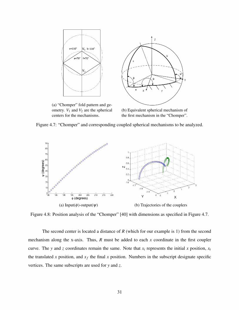
(a) “Chomper” fold pattern and ge-ometry. V1 and V2 are the sphericalcenters for the mechanisms.

(b) Equivalent spherical mechanism ofthe first mechanism in the “Chomper”.

Figure 4.7: “Chomper” and corresponding coupled spherical mechanisms to be analyzed.

(a) Input(φ )-output(ψ) (b) Trajectories of the couplers

Figure 4.8: Position analysis of the “Chomper” [40] with dimensions as specified in Figure 4.7.

The second center is located a distance of R (which for our example is 1) from the second

mechanism along the x-axis. Thus, R must be added to each x coordinate in the first coupler

curve. The y and z coordinates remain the same. Note that xi represents the initial x position, xt

the translated x position, and x f the final x position. Numbers in the subscript designate specific

vertices. The same subscripts are used for y and z.

31

xt = xi +R (4.15)

yt = yi (4.16)

zt = zi (4.17)

Next the translated coupler curve must be rotated 180 degrees. This is accomplished us-

ing the following equations for rotations of cartesian coordinates about the z-axis (because the

mechanism centers are fixed, the z-axis is also fixed thus the rotation are fairly simple):

x f = xt ∗ cos(θ)− yt ∗ sin(θ) (4.18)

y f = xt ∗ sin(θ)+ yt ∗ cos(θ) (4.19)

z f = zt (4.20)

For this example, θ = 180◦, thus the above simplifies to:

x2 f =−x1t (4.21)

y2 f =−y1t (4.22)

z2 f = z1t (4.23)

The path of the coupler points of both mechanisms is presented in Figure 4.8b. From this

we see the expected motion of the two sides converging. The motion of the two couplers at several

points throughout their motion is shown in Figure 4.9.

4.4.2 Loop

The “Square Twist” model is composed of four identical spherical mechanisms coupled in

such a manner that they form a loop (Figure 4.10a). A traditional kinematic representation of the

spherical mechanism located at the origin is found in Figure 4.10b. Note that one center is located

32

(a) φ = 181◦ (b) φ = 193◦

(c) φ = 205◦ (d) φ = 217◦

Figure 4.9: Path of the coupler links for the “Chomper”.

a distance of 1 from the origin (again using the unit sphere) in the y-direction and is rotated by -90◦.

The next center (moving clockwise around the loop) is located a distance of 1 in both the x- and

y-directions and is rotated 180◦. The last mechanism is located a distance of 1 in the x-direction

from the origin and is rotated by 90◦. By leveraging symmetry, one of these mechanisms can be

solved and that solution can be translated and rotated to the other three spherical centers.

Solving the first spherical mechanism yields the input-output relationship found in Fig-

ure 4.11a. The input-output relationship of the remaining three mechanisms is similar to that of

the first. Translating the coupler curve from the first mechanism to the second and rotating by -90

degrees is accomplished using the following translations:

33

(a) “Square Twist” fold pattern andgeometry. V1, V2, V3, and V4 are thespherical centers.

(b) Equivalent spherical mechanism of the firstmechanism in the square twist.

Figure 4.10: “Square Twist” and corresponding loop of spherical mechanisms to be analyzed.

(a) Input(φ )-output(ψ) (b) Trajectories of the couplers

Figure 4.11: Position analysis of the “Square Twist”.

x2t = x1i (4.24)

y2t = y1i +R (4.25)

z2t = z1i (4.26)

34

and the following rotations:

x2 f = y2t (4.27)

y2 f =−x2t (4.28)

z2 f = z2t (4.29)

Moving the coupler curve to the third spherical center is accomplished by the following

translations:

x3t = x1i +R (4.30)

y3t = y1i +R (4.31)

z3t = z1i (4.32)

and next the following rotations.

x3 f =−x3t (4.33)

y3 f =−y3t (4.34)

z3 f = z3t (4.35)

Moving the coupler curve to the fourth spherical center is accomplished by first translating

as follows:

x4t = x1i +R (4.36)

y4t = y1i (4.37)

z4t = z1i (4.38)

35

then rotating, as follows:

x4 f =−y4t (4.39)

y4 f = x4t (4.40)

z4 f = z4t (4.41)

The paths of the overall mechanism is presented in Figure 4.11b. The motion of the four

couplers at several angles is shown in Figure 4.12. When actuated from the edges, the center square

of this models twists. When the center is fixed, the twist is imparted to the coupler links.

4.5 Future work

The method that has been described and demonstrated above simplifies the solution of

systems of identical spherical mechanisms whose centers are attached to a ground link. Not all

action origami fits within these restrictions. An example exception is Shafer’s “Frog’s Tongue”

model [41] shown in Figure 4.13a. When a panel is chosen as ground and the model is actuated,

spherical centers along the center of the model move through space. In the examples performed

above the spherical centers were always fixed. When the centers are allowed to move, the analysis

becomes more complex.

2D Periodic models such as the “Miura-Ori” [50] fold (Figure 4.13b) also have moving

centers that require a more advanced version of the method outlined here.

4.6 Conclusion

Utilizing the knowledge that much of action origami is composed of spherical mechanisms

allows the use of traditional kinematic equations for understanding the behavior of these systems.

Every origami vertex is a spherical change point mechanism whose links sum to 360◦. A position

analysis of a single origami vertex was performed, resulting in a relationship between input and

output angles as well as the path of the coupler link.

36

(a) φ = 1◦ (b) φ = 60◦

(c) φ = 120◦ (d) φ = 179◦

Figure 4.12: Path of the coupler links for the “Square Twist”.

In coupled systems of spherical mechanisms, if the mechanisms are identical (i.e. have the

same link lengths) and the spherical centers are grounded, one of the mechanisms can be solved

and the results applied to each vertex. In particular, the coupler curve can be moved from the

solved mechanism to every other using translations and rotations to understand the overall motion

of the system. Taking advantage of symmetry in this manner results in a significant reduction of

computation time for large, multi-vertex models.

Future work can be done to perform velocity and acceleration analyses, in addition to mo-

tion, path, and function generation. The capabilities of the presented method could also be ex-

37

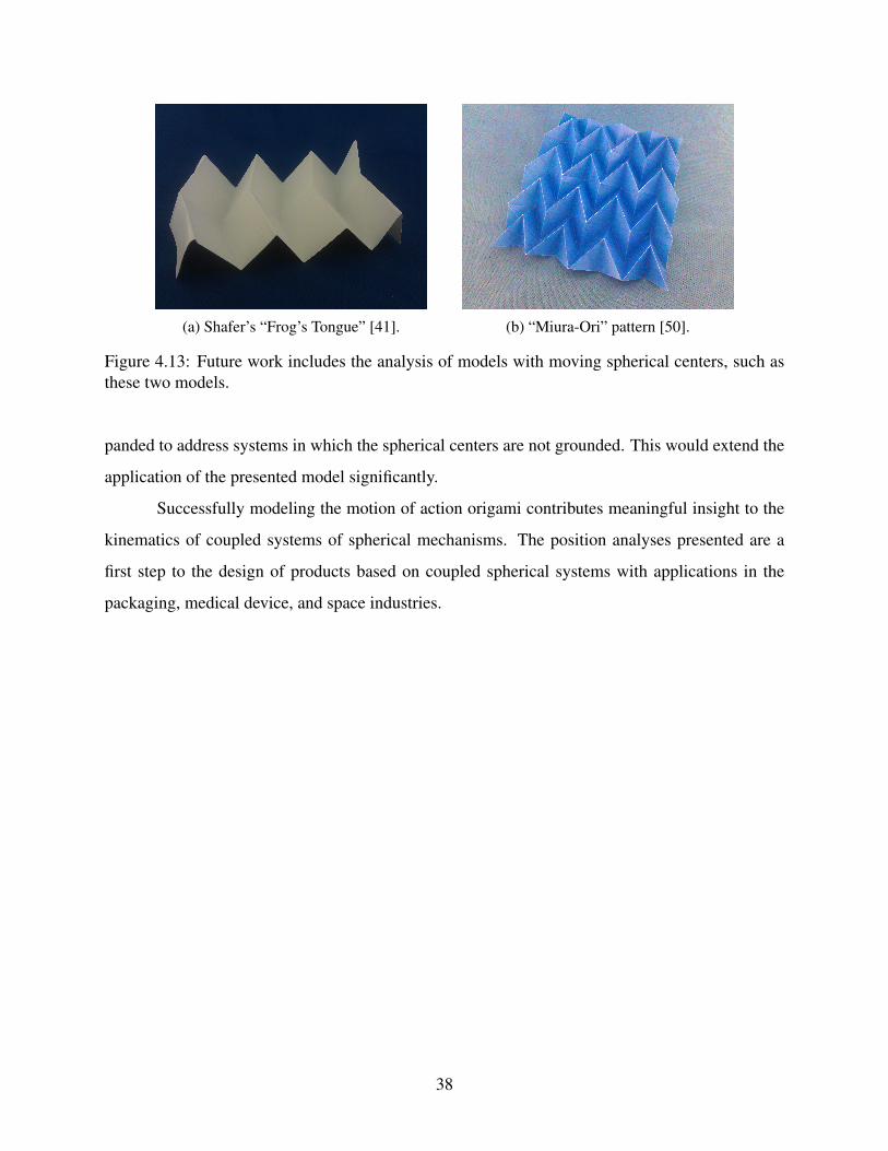
(a) Shafer’s “Frog’s Tongue” [41]. (b) “Miura-Ori” pattern [50].

Figure 4.13: Future work includes the analysis of models with moving spherical centers, such asthese two models.

panded to address systems in which the spherical centers are not grounded. This would extend the

application of the presented model significantly.

Successfully modeling the motion of action origami contributes meaningful insight to the

kinematics of coupled systems of spherical mechanisms. The position analyses presented are a

first step to the design of products based on coupled spherical systems with applications in the

packaging, medical device, and space industries.

38

CHAPTER 5. CONCLUSION

5.1 Conclusions

The main conclusion for this thesis is that viewing action origami as spherical mechanisms

is a useful tool that yields two advantages.

1. It allows for a systematic and simple method of classification of action origami, and by

extension systems of spherical mechanisms. This was demonstrated in Chapter 3.

2. Spherical mechanisms advances can be leveraged to understand the kinematics of compli-

cated action origami models. A first step in demonstrating the power of this understanding

was presented in Chapter 4.

The literature review that was performed shows that there is a profusion of literature about

origami in many fields. It is likely that future problems encountered in origami-inspired design

have already been thought about, but in an entirely different field than expected. It is hoped that

the brief summary of origami literature found in Chapter 2 and the references found in the Bibli-

ography would be of assistance to those searching for solutions to such problems.

5.2 Future Work

As has been stated, the work that was done in this thesis is but a first step to understanding

and implementing coupled systems of spherical mechanisms into the design of mechanisms. There

are three areas in particular that could benefit from further work.

1. A more complete kinematic analysis of the mechanisms described in Chapter 4 would be

of great worth to those desiring to optimize a design dealing with coupled spherical mecha-

nisms. In particular, velocity and acceleration analyses would increase what is known about

39

the kinematics of those mechanisms. Path, motion, and function generation would allow for

meaningful implementation in more complicated applications.

2. The method proposed in Chapter 4 was demonstrated for systems of spherical mechanisms

in which all spherical centers were fixed to ground. While this is not uncommon, there

are many models in which all centers cannot be fixed, thus they move through space when

subjected to an input motion. Furthering the method to allow for such models would be of

great importance. It is hypothesized that the motion of such models could be viewed using

superposition. The motion of the mechanism centers through space could be solved, after

which the motion of each spherical center could be solved at each location. If all mechanisms

are the same, as they often are in tesselations, one mechanism could be solved and the results

translated and rotated to every other center.

3. Lastly, discovering areas of application is extremely important in order to demonstrate the

unique capabilities of action origami-based designs, namely flat-foldability, deployability,

and sophisticated motion while in the deployed state. Minimally invasive surgery and de-

ployable space arrays are possible application areas, but there are many other areas such

mechanisms could contribute to.

40

REFERENCES

[1] Baranger, E., Guidault, P., and Cluzel, C. “Numerical modeling of the geometrical defects ofan origami-like sandwich core.” Composite Structures, 93. 4, 8

[2] Benjeddou, O., Limam, O., and Ouezdou, M. “Experimental and theoretical study of a fold-able composite beam.” Engineering Structures, 44. 4

[3] Yao, W., and Dai, J., 2008. “Dexterous manipulation of origami cartons with robotic fingersbased on the interactive configuration space.” Journal of Mechanical Design, 130(022303),February. 4, 6, 10, 24

[4] In, H., Kumar, S., Shao-Horn, Y., and Barbastanthis, G., 2006. “Origami fabrication of nanos-tructured, three-dimensional devices: Electrochemical capacitors with carbon electrodes.”Applied Physics Letters, 88(083104), February. 4, 6, 8

[5] Heller, A., 2003. “A giant leap for space telescopes.” Science & Technology Review, pp. 12–18. 4, 22

[6] Cromvik, C., 2007. “Numerical folding of airbags based on optimization and origami.” Mas-ter’s thesis, Chalmers University of Technology and Goteborg University. 4, 22

[7] Peoplow, M., 2004. Japanese deploy solar sails. 4

[8] Fozzils, 2013. Fozzils home page. 4

[9] Kayak, O., 2013. Oru kayak home page. 4

[10] You, Z., and Kuribayashi, K., 2003. “A novel origami stent.” In 2003 Summer BioengineeringConference, Vol. , pp. 257–258. 4

[11] Ma, J., and You, Z., 2010. “The origami crash box.” In The 5th International Conference onOrigami in Science, Mathematics, and Education. 4, 22

[12] Architizer, 2013. Folding architecture: Top 10 origami-inspired buildings. 4

[13] Dureisseix, D., 2012. “An overview of mechanisms and patterns with origami.” InternationalJournal of Space Systems, 27(1), pp. 1–14. 4

[14] Hawkes, E., An, B., Benbernou, N., Tanaka, H., Kim, S., Demaine, E., Rus, D., and Wood,R., 2010. “Programmable matter by folding.” In Proceedings of the National Academy ofSciences, G. Strang, ed., Vol. 107, PNAS, PNAS, pp. 12441–12445. 5

[15] Etherington, R., 2012. Hydro-fold by christope guberan. 5

41

[16] Ryu, J., D’Amato, M., Cui, X., Long, K., Qi, H., and Dunn, M., 2012. “Photo-origami—bending and folding polymers with light.” Applied Physics Letters, 100(161908), April. 5

[17] An, B., Benbernou, N., Demaine, E., and Rus, D. “Planning to fold multiple objects from asingle self-folding sheet.” Robotica, 29. 5

[18] Ahmed, S., Lauff, C., Crivaro, A., McGough, K., Sheridan, R., Frecker, M., von Lock-ette, P., Ounaies, Z., Simpson, T., Ling, J., and Strzelec, R., 2013. “Multi-field responsiveorigami structures; preliminary modeling and experiments.” In Proceedings of the ASME2013 IDETC/CIE Conference. 5

[19] Tachi, T., 2009. “Simulation of rigid origami.” In Origami 4: Fourth International Meetingof Origami Science, Mathematics, and Education, R. Lang, ed., Vol. , A K Peters, Ltd.,pp. 175–188. 5, 10, 22, 24

[20] Wang, K., and Chen, Y., 2011. “Folding a patterned cylinder by rigid origami.” In Origami5: Fifth International Meeting of Origami Science, Mathematics, and Education, P. Wang-Iverson, R. Lang, and M. Yim, eds., Vol. , CRC Press, pp. 265–276. 5, 10, 24

[21] Tachi, T., 2011. “Rigid-foldable thick origami.” In Origami 5: Fifth International Meeting ofOrigami Science, Mathematics, and Education, P. Wang-Iverson, R. Lang, and M. Yim, eds.,Vol. , CRC Press, pp. 253–264. 5

[22] Hoberman, C., 2010. Folding structures made of thick hinged panels, 09. 6

[23] Liu, H., and Dai, J., 2002. “Kinematics and mobility analysis of carton folds in packingmanipulation based on the mechanism equivalent.” In Proceedings of the Institution of Me-chanical Engineers Part C: Journal of Mechanical Engineering Science, Vol. 216, Institutionof Mechanical Engineers, pp. 959–970. 6, 10, 24

[24] Zhang, K., Dai, J., and Fang, Y., 2010. “Topology and constraint analysis of phase changein the metamorphic chain and its evolved mechanism.” Journal of Mechanical Design,132(121001), December. 6

[25] Balkcom, D., and Mason, M. “Robotic origami folding.” The International Journal ofRobotics Research, 27. 6, 10, 23, 24

[26] Chiang, C., 1988. Kinematics of Spherical Mechanisms. Cambridge University Press, June.6, 24, 26

[27] Wu, W., and You, Z., 2010. “Modelling rigid origami with quaternions and dual quaternions.”The Royal Society, 466, pp. 2155–2174. 6, 24

[28] Furuta, Y., Mitani, J., and Fukui, Y., 2008. “Modeling and animation of 3d origami usingspring mass simulation.” In Proceedings of NICOGRAPH. 6, 24

[29] s. belecastro, and Hull, T., 2002. “Modelling the folding of paper into three dimensions usingaffine transformations.” Linear Algebra and its applications, 348, pp. 273–282. 6, 24

[30] Dai, J., and Cannella, F., 2007. “Stiffness characteristics of carton folds for packaging.”Journal of Mechanical Design, 130(022305), December. 6

42

[31] Jurga, S., Hidrovo, C., Niemczura, J., Smith, H., and Barbastathis, G., 2003. “Nanostructuredorigami.” In Nanotechnology, 2003. IEEE-NANO 2003. 2003 Third IEEE Conference on,Vol. 1, IEEE, pp. 220–223. 6

[32] Durney, M., Pendley, A., and Rappaport, I., 2006. Techniques for designing and manufactur-ing precision-folded high strength, fatigue-resistant structures and sheet therefore, 12. 7

[33] Durney, M., and Pendley, A., 2002. Method for precision bending of sheet of materials, slitsheets fabrication process, 4. 7

[34] Bern, M., and Hayes, B., 1966. “The complexity of flat origami.” In Proceedings of theseventh annual ACM-SIAM symposium on discrete algorithms, Vol. , Society for Industrialand Applied Mathematics, pp. 175–183. 7

[35] Demaine, E., and O’Rourke, J., 2007. Geometric folding algorithms. Cambridge UniversityPress Cambridge. 7

[36] Hull, T., 1994. “On the mathematics of flat origamis.” Congressus Numerantium, pp. 215–224. 7

[37] Lang, R., 1996. “A computational algorithm for origami design.” In Proceedings of thetwelfth annual symposium on Computational geometry, ACM, pp. 98–105. 7, 22

[38] Lang, R., 1997. Origami in Action: Paper Toys That Fly, Flap, Gobble, and Inflate!. St.Martin’s Press, New York, NY. 7, 11, 13, 15, 16

[39] Lang, R., 1988. The Complete Book of Origami. Dover Publications Inc., New York, NY. 7,11

[40] Shafer, J., 2010. Origami Ooh La La!: Action Origami for Performance and Play. J. Shafer.viii, 7, 9, 11, 18, 25, 30, 31

[41] Shafer, J., 2001. Origami to Astonish and Amuse. St. Martin’s Press, New York, NY. viii, 7,9, 11, 16, 17, 22, 36, 38

[42] Greenberg, H., 2012. “The Application of Origami to the Design of Lamina Emergent Mech-anisms (LEMs) with Extensions to Collapsible, Compliant, and Flat Folding Mechanisms.”MS Thesis, Brigham Young University, Provo, UT. 10

[43] Greenberg, H., Gong, M., Magleby, S., and Howell, L. “Indentifying links between origamiand compliant mechanisms.” Mechanical Sciences, 2. 10

[44] Winder, B., Magleby, S., and Howell, L., 2009. “Kinematic representations of pop-up papermechanisms.” Journal of Mechanisms and Robotics, 1(2). 10

[45] Schenk, M., and Guest, S., 2011. “Origami folding: A structural engineering approach.” InOrigami 5: Fifth International Meeting of Origami Science, Mathematics, and Education,P. Wang-Iverson, R. Lang, and M. Yim, eds., Vol. , CRC Press, pp. 291–304. 10

[46] Demaine, E., and O’Rourke, J., 2007. Geometric Folding Algorithms: Linkages, Origami,Polyhedra. Cambridge University Press, New York, NY. 10

43

[47] Weisstein, E. Vertex degree On Mathworld — A Wolfram Web Resource URLwww.mathworld.wolfram.com/VertexDegree. 10

[48] Stachel, H., 2006. “A kinematic approach to kokotsakis meshes.” Computer Aided GeometricDesign, 88(083104), February. 10, 24

[49] Wilding, S. “Spherical lamina emergent mechanisms.” Mechanism and Machine Theory, 49.10, 24

[50] Miura, M., 2002. “The application of origami science to map and atlas design.” In Origami3: Third International Meeting of Origami Science, Mathematics, and Education, T. Hull,ed., Vol. , CRC Press, pp. 137–146. 17, 36, 38

[51] Bowen, L., Grames, C., Magleby, S., Lang, R., and Howell, L. L., 2013. “An approach forunderstanding action origami as kinematic mechanisms.” In Proceedings of the ASME 2013IDETC/CIE Conference. 23, 24

[52] Makhsudyan, N., Djavakhyan, V., and Arakelin, V., 2009. “Comparative analysis and syn-thesis of six-bar mechanisms formed by two serially connected spherical and planar four-barlinkages.” Mechanics Research Communications, 36, pp. 162–168. 23

[53] Dzhavakhyan, R., Makhsudyan, N., and Arakelyan, V., 2011. “Comparative analysis andsynthesis of plane and spherical four hinge mechanisms.” Journal of Machinery Manufactureand Reliability, 40, pp. 423–429. 23

[54] Greenberg, H., Gong, M., Magleby, S., and Howell, L., 2011. “Identifying links betweenorigami and compliant mechanisms.” Mechanical Sciences, 2, pp. 217–225. 23

[55] Jacobsen, J., Winder, B., Howell, L., and Magleby, S., 2010. “Lamina emergent mechanismsand their basic elements.” Journal of Mechanisms and Robotics, 2(1), pp. 1–9. 24

[56] Wei, G., and Dai, J., 2009. “Geometry and kinematic analysis of an origami-evolved mecha-nism based on artmimetics.” In ASME/IFToMM. 24

[57] Cervantes-Sanchez, J. J., and Medellın-Castillo, H. I., 2002. “A robust classification schemefor spherical 4R linkages.” Mechanism and Machine Theory, 37(10), Oct., pp. 1145–1163.24, 27

[58] Chu, J., and Sun, J., 2007. “Synthesis of coupler curves of spherical four-bar mechanismthrough fast fourier transform.” In 12th IFToMM World Congress. 24, 27

[59] Larochelle, P., Dooley, J., Murray, A., and McCarthy, J., 1993. “SPHINX - Software forsynthesizing spherical mechanisms.” In NSF Design and Manufacturing Systems ConferenceProceedings of the 1993 NSF Design and Manufacturing Systems Conference. 24

44

APPENDIX A. MATLAB POSITION ANALYSIS PROGRAMS

A.1 Required Functions

A.1.1 Spherical Four Bar (s4bar.m)

%This function calculates the two possible output angles of a spherical

%4bar for a given input angle. See page 8 of C.H. Chiang's Kinematics of

%Spherical Mechanisms. Also it calculates the x, y, z coordinates of a

%coupler point

%a=input link angle(length)

%b=output link angle

%c=coupler link angle

%f=ground link angle

%phi=input angle

%See "Kinematics of Spherical Mechanisms" by C.H.Chiang for phi(input

%angle) and psi(output angle)

%x axis is defined positive from center of spherical mechanism through the

%joint connecting the input and ground, y 90 degrees CCW, z up

%Note that all inputs to this function are in degrees

function [vals] = s4bar(a,b,c,f,phi)

%convert to radians

a = a*pi/180;

b = b*pi/180;

c = c*pi/180;

f = f*pi/180;

phi = phi*pi/180;

%intermediate step

k1 = cos(a)*cos(b)*cos(f);

k2 = cos(c);

45

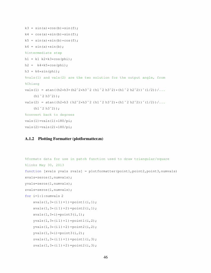
k3 = sin(a)*cos(b)*sin(f);

k4 = cos(a)*sin(b)*sin(f);

k5 = sin(a)*sin(b)*cos(f);

k6 = sin(a)*sin(b);

%intermediate step

h1 = k1 k2+k3*cos(phi);

h2 = k4+k5*cos(phi);

h3 = k6*sin(phi);

%vals(1) and vals(2) are the two solution for the output angle, from

%Chiang

vals(1) = atan((h2*h3+(h2ˆ2*h3ˆ2 (h1ˆ2 h3ˆ2)*(h1ˆ2 h2ˆ2))ˆ(1/2))/...

(h1ˆ2 h3ˆ2));

vals(2) = atan((h2*h3 ( h2ˆ2*h3ˆ2 (h1ˆ2 h3ˆ2)*(h1ˆ2 h2ˆ2))ˆ(1/2))/...

(h1ˆ2 h3ˆ2));

%convert back to degrees

vals(1)=vals(1)*180/pi;

vals(2)=vals(2)*180/pi;

A.1.2 Plotting Formatter (plotformatter.m)

%formats data for use in patch function used to draw triangular/square

%links May 30, 2013

function [xvals yvals zvals] = plotformatter(point1,point2,point3,numvals)

xvals=zeros(1,numvals);

yvals=zeros(1,numvals);

zvals=zeros(1,numvals);

for i=1:1:numvals 2

xvals(1,3*(i1)+1)=point1(i,1);

xvals(1,3*(i1)+2)=point2(i,1);

xvals(1,3*i)=point3(i,1);

yvals(1,3*(i1)+1)=point1(i,2);

yvals(1,3*(i1)+2)=point2(i,2);

yvals(1,3*i)=point3(i,2);

zvals(1,3*(i1)+1)=point1(i,3);

zvals(1,3*(i1)+2)=point2(i,3);

46

zvals(1,3*i)=point3(i,3);

end

A.2 Single

A.2.1 Single Coupler Path (SinglePath.m)

%This program performs several function for a single spherical mechanism:

%1. Solves for the output angles and plots the input output relationship

%2. Solves for internal angle beta and plots the input beta relationship

%3. Solves for and plots the x,y,z components of a coupler point

%May 29, 2013

clear all

clc

close all

%definitions

%start angle

s angle = 1;

%end angle

e angle = 179;

%increment

incr = 1;

%calculate number of points

numpoints = (e angle s angle)/incr;

%allocate space

output angles = zeros(numpoints,2);

output angles rads = zeros(numpoints,2);

couplerpoint = zeros(numpoints,3);

joint1 = zeros(numpoints,3);

joint2 = zeros(numpoints,3);

couplerpointR = zeros(numpoints,3);

Beta = zeros(numpoints,1);

Beta deg = zeros(numpoints,1);

%define link lengths in degrees

a=45; %input

47

b=135; %output

c=45; %coupler

f=135; %ground

%define coupler information

thetap=0;

theta0=30;

RP=1.5;

R=1;

for i=s angle : incr : e angle

%the inputs are (a,b,c,f,phi)

vals = s4bar(a,b,c,f,i);

output angles(i ( s angle 1),1) = vals(1);

output angles(i ( s angle 1),2) = vals(2);

end

input angles = s angle:incr:e angle;

%this is temporary hopefully, adjusts output so all angles are positive,

%note that adding 180 is not tecnically accurate as we start at 1 degree

%Don't know where 70 comes from...that is just where it was discontinuous

for i=1:1:70

output angles(i,2) = output angles(i,2)+180;

end

%convert to radians

a = a*pi/180;

b = b*pi/180;

c = c*pi/180;

f = f*pi/180;

thetap = thetap*pi/180;

theta0 = theta0*pi/180;

%convert output back into radians for use in beta equation

for i=s angle : incr : e angle

output angles rads(i ( s angle 1),1)=output angles(i ( s angle 1),2)...

*pi/180;

end

%calculate beta for each angle

48

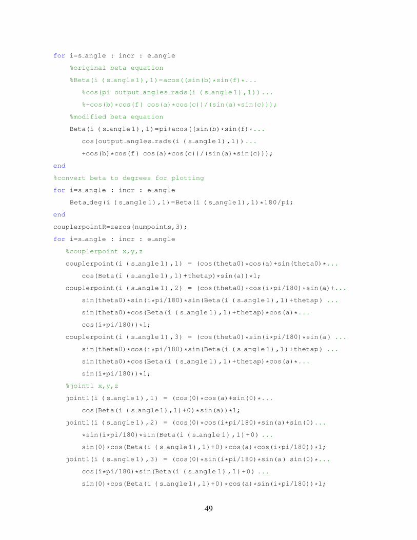
for i=s angle : incr : e angle

%original beta equation

%Beta(i ( s angle 1),1)=acos((sin(b)*sin(f)*...

%cos(pi output angles rads(i ( s angle 1),1))...

%+cos(b)*cos(f) cos(a)*cos(c))/(sin(a)*sin(c)));

%modified beta equation

Beta(i ( s angle 1),1)=pi+acos((sin(b)*sin(f)*...

cos(output angles rads(i ( s angle 1),1))...

+cos(b)*cos(f) cos(a)*cos(c))/(sin(a)*sin(c)));

end

%convert beta to degrees for plotting

for i=s angle : incr : e angle

Beta deg(i ( s angle 1),1)=Beta(i ( s angle1),1)*180/pi;

end

couplerpointR=zeros(numpoints,3);

for i=s angle : incr : e angle

%couplerpoint x,y,z

couplerpoint(i ( s angle 1),1) = (cos(theta0)*cos(a)+sin(theta0)*...

cos(Beta(i ( s angle 1),1)+thetap)*sin(a))*1;

couplerpoint(i ( s angle 1),2) = (cos(theta0)*cos(i*pi/180)*sin(a)+...

sin(theta0)*sin(i*pi/180)*sin(Beta(i ( s angle 1),1)+thetap) ...

sin(theta0)*cos(Beta(i ( s angle 1),1)+thetap)*cos(a)*...

cos(i*pi/180))*1;

couplerpoint(i ( s angle 1),3) = (cos(theta0)*sin(i*pi/180)*sin(a) ...

sin(theta0)*cos(i*pi/180)*sin(Beta(i ( s angle 1),1)+thetap) ...

sin(theta0)*cos(Beta(i ( s angle 1),1)+thetap)*cos(a)*...

sin(i*pi/180))*1;

%joint1 x,y,z

joint1(i ( s angle 1),1) = (cos(0)*cos(a)+sin(0)*...

cos(Beta(i ( s angle1),1)+0)*sin(a))*1;

joint1(i ( s angle 1),2) = (cos(0)*cos(i*pi/180)*sin(a)+sin(0)...

*sin(i*pi/180)*sin(Beta(i ( s angle 1) ,1)+0) ...

sin(0)*cos(Beta(i ( s angle1),1)+0)*cos(a)*cos(i*pi/180))*1;

joint1(i ( s angle 1),3) = (cos(0)*sin(i*pi/180)*sin(a) sin(0)*...

cos(i*pi/180)*sin(Beta(i ( s angle 1) ,1)+0) ...

sin(0)*cos(Beta(i ( s angle1),1)+0)*cos(a)*sin(i*pi/180))*1;

49

%joint2 x,y,z

joint2(i ( s angle 1),1) = (cos(c)*cos(a)+sin(c)*...

cos(Beta(i ( s angle1),1)+0)*sin(a))*1;

joint2(i ( s angle 1),2) = (cos(c)*cos(i*pi/180)*sin(a)+sin(c)...

*sin(i*pi/180)*sin(Beta(i ( s angle 1) ,1)+0) ...

sin(c)*cos(Beta(i ( s angle1),1)+0)*cos(a)*cos(i*pi/180))*1;

joint2(i ( s angle 1),3) = (cos(c)*sin(i*pi/180)*sin(a) sin(c)*...

cos(i*pi/180)*sin(Beta(i ( s angle 1) ,1)+0) ...

sin(c)*cos(Beta(i ( s angle1),1)+0)*cos(a)*sin(i*pi/180))*1;

%Coupler Point R x,y,z

couplerpointR(i ( s angle 1),1) = (cos(theta0)*cos(a)+sin(theta0)*...

cos(Beta(i ( s angle1),1))*sin(a))*RP;

couplerpointR(i ( s angle 1),2) = (cos(theta0)*cos(i*pi/180)*...

sin(a)+sin(theta0)*sin(i*pi/180)*sin(Beta(i ( s angle 1) ,1)) ...

sin(theta0)*cos(Beta(i ( s angle1),1))*cos(a)*cos(i*pi/180))*RP;

couplerpointR(i ( s angle 1),3) = (cos(theta0)*sin(i*pi/180)*sin(a)...

sin(theta0)*cos(i*pi/180)*sin(Beta(i ( s angle 1) ,1)) ...

sin(theta0)*cos(Beta(i ( s angle1),1))*cos(a)*sin(i*pi/180))*RP;

end

%Plotting!

%plot for 1st solution

subplot(3,1,1)

scatter(input angles',output angles(:,1))

xlabel('Input angle (degrees)')

ylabel('Output angle (degrees)')

%plot for second solution

subplot(3,1,2)

scatter(input angles',output angles(:,2))

xlabel('Input angle (degrees)')

ylabel('Output angle (degrees)')

%plot beta

subplot(3,1,3)

scatter(input angles',Beta deg(:,1))

xlabel('Input angle (degrees)')

ylabel('Beta (degrees)')

figure(2)

50

subplot(2,2,1)

scatter3(couplerpointR(:,1),couplerpointR(:,2),couplerpointR(:,3))

title('Trajectory of Coupler Point R');

xlabel('X');

ylabel('Y');

zlabel('Z');

subplot(2,2,2)

scatter3(couplerpoint(:,1),couplerpoint(:,2),couplerpoint(:,3))

title('Trajectory of Coupler Point');

xlabel('X');

ylabel('Y');

zlabel('Z');

subplot(2,2,3)

scatter3(joint1(:,1),joint1(:,2),joint1(:,3))

title('Trajectory of Joint1');

xlabel('X');

ylabel('Y');

zlabel('Z');

subplot(2,2,4)

scatter3(joint2(:,1),joint2(:,2),joint2(:,3))

title('Trajectory of Joint2');

xlabel('X');

ylabel('Y');

zlabel('Z');

A.2.2 Single Coupler Motion (SingleMotion.m)

%This program demonstrates the motion of the coupler link for a single

%spherical mechanism. Coupler member shown is a triangle defined by joints

%on either side of the coupler link at a radius defined by R and a coupler

%point defined by thetap and RP.

%May 29, 2013

clear all

clc

close all

51

s angle = 1;

e angle = 179;

incr = 1;

numpoints = (e angle s angle)/incr;

output angles = zeros(numpoints,2);

output angles rads = zeros(numpoints,2);

couplerpoint = zeros(numpoints,3);

couplerpoint1 = zeros(numpoints,3);

couplerpoint2 = zeros(numpoints,3);

couplerpointR = zeros(numpoints,3);

Beta = zeros(numpoints,1);

dP = zeros(numpoints,2);

%define link lengths in degrees

a=45; %input

b=135; %output

c=45; %coupler

f=135; %ground

%define coupler information

thetap=0;

theta0=30;

RP=1.5;

R=1;

for i=s angle : incr : e angle

vals = s4bar(a,b,c,f,i);

output angles(i ( s angle 1),1) = vals(1);

output angles(i ( s angle 1),2) = vals(2);

end

input angles = s angle:incr:e angle;

%this is temporary hopefully, adjusts output so all angles are positive,

%note that adding 180 is not tecnically accurate as we start at 1 degree

%Don't know where 70 comes from...that is just where it was discontinuous

for i=1:1:70

output angles(i,2) = output angles(i,2)+180;

end

%define link lengths, etc, convert to radians

a = a*pi/180;

52

b = b*pi/180;

c = c*pi/180;

f = f*pi/180;

thetap = thetap*pi/180;

theta0 = theta0*pi/180;

%convert output back into radians for use in beta equation

for i=s angle : incr : e angle

output angles rads(i ( s angle 1),1)=output angles(i ( s angle 1),2)*...

pi/180;

end

%calculate beta for each angle, note that we should technically have

%cos(pi output ...), also shouldn't have the pi in front

for i=s angle : incr : e angle

%Beta(i ( s angle 1),1)=acos((sin(b)*sin(f)*...

%cos(pi output angles rads(i ( s angle1),1))+...

%cos(b)*cos(f) cos(a)*cos(c))/(sin(a)*sin(c)));

Beta(i ( s angle 1),1)=pi+acos((sin(b)*sin(f)*...

cos(output angles rads(i ( s angle1),1))+cos(b)*cos(f) cos(a)*...

cos(c))/(sin(a)*sin(c)));

end

Beta deg = zeros(numpoints,1);

%convert beta to degrees for plotting

for i=s angle : incr : e angle

Beta deg(i ( s angle 1),1)=Beta(i ( s angle1),1)*180/pi;

end

for i=s angle : incr : e angle

%couplerpoint

couplerpoint(i ( s angle 1),1) = (cos(theta0)*cos(a)+sin(theta0)*...

cos(Beta(i ( s angle 1),1)+thetap)*sin(a))*R;

couplerpoint(i ( s angle 1),2) = (cos(theta0)*cos(i*pi/180)*...

sin(a)+sin(theta0)*sin(i*pi/180)*sin(Beta(i ( s angle 1),1)+...

thetap) sin(theta0)*cos(Beta(i ( s angle 1),1)+thetap)*...

cos(a)*cos(i*pi/180))*R;

couplerpoint(i ( s angle 1),3) = (cos(theta0)*sin(i*pi/180)*sin(a) ...

sin(theta0)*cos(i*pi/180)*sin(Beta(i ( s angle 1),1)+thetap) ...

sin(theta0)*cos(Beta(i ( s angle 1),1)+thetap)*cos(a)*...

53

sin(i*pi/180))*R;

%joint1

couplerpoint1(i ( s angle 1),1) = (cos(0)*cos(a)+sin(0)*...

cos(Beta(i ( s angle1),1)+0)*sin(a))*R;

couplerpoint1(i ( s angle 1),2) = (cos(0)*cos(i*pi/180)*sin(a)+...

sin(0)*sin(i*pi/180)*sin(Beta(i ( s angle 1) ,1)+0) ...

sin(0)*cos(Beta(i ( s angle1),1)+0)*cos(a)*cos(i*pi/180))*R;

couplerpoint1(i ( s angle 1),3) = (cos(0)*sin(i*pi/180)*sin(a) ...

sin(0)*cos(i*pi/180)*sin(Beta(i ( s angle 1) ,1)+0) ...

sin(0)*cos(Beta(i ( s angle1),1)+0)*cos(a)*sin(i*pi/180))*R;

%joint2

couplerpoint2(i ( s angle 1),1) = (cos(c)*cos(a)+sin(c)*...

cos(Beta(i ( s angle1),1)+0)*sin(a))*R;

couplerpoint2(i ( s angle 1),2) = (cos(c)*cos(i*pi/180)*sin(a)+...

sin(c)*sin(i*pi/180)*sin(Beta(i ( s angle 1) ,1)+0) ...

sin(c)*cos(Beta(i ( s angle1),1)+0)*cos(a)*cos(i*pi/180))*R;

couplerpoint2(i ( s angle 1),3) = (cos(c)*sin(i*pi/180)*sin(a) ...

sin(c)*cos(i*pi/180)*sin(Beta(i ( s angle 1) ,1)+0) ...

sin(c)*cos(Beta(i ( s angle1),1)+0)*cos(a)*sin(i*pi/180))*R;

%Coupler Point R

couplerpointR(i ( s angle 1),1) = (cos(theta0)*cos(a)+sin(theta0)*...

cos(Beta(i ( s angle1),1))*sin(a))*RP;

couplerpointR(i ( s angle 1),2) = (cos(theta0)*cos(i*pi/180)*sin(a)+...

sin(theta0)*sin(i*pi/180)*sin(Beta(i ( s angle 1) ,1)) ...

sin(theta0)*cos(Beta(i ( s angle1),1))*cos(a)*cos(i*pi/180))*RP;

couplerpointR(i ( s angle 1),3) = (cos(theta0)*sin(i*pi/180)*sin(a) ...

sin(theta0)*cos(i*pi/180)*sin(Beta(i ( s angle 1) ,1)) ...

sin(theta0)*cos(Beta(i ( s angle1),1))*cos(a)*sin(i*pi/180))*RP;

end

xvals=zeros(1,numpoints);

yvals=zeros(1,numpoints);

zvals=zeros(1,numpoints);

[xvals,yvals,zvals]=plotformatter(couplerpointR,couplerpoint1,...

couplerpoint2,numpoints);

xvals=xvals';

yvals=yvals';

54

zvals=zvals';

xvals2=zeros(1,numpoints);

yvals2=zeros(1,numpoints);

zvals2=zeros(1,numpoints);

[xvals2,yvals2,zvals2]=plotformatter(couplerpoint,couplerpoint1,...

couplerpoint2,numpoints);

xvals=xvals';

yvals=yvals';

zvals=zvals';

%figure

for i=1:1:numpoints 2

%sets the view of the graph. The first number is the azimuth

%(horizontal rotation about the z axis). The second is the elevation

view(130,30)

%sets the x y z axes to prevent autoscaling [xmin xmax ymin ymax...]

axis([ 1 2 2 2 0 2]);

axis manual

%starts the plot in 3D view

axis vis3d

%creates ground link triangle from 3 points [x1,x2,x3],[y1,y2,y3]

patch([0,1,sin(pi/4)],[0,0,sin(pi/4)],[0,0,0],'r');

%creates coupler link

patch(xvals(3*(i1)+1:3*i),yvals(3*(i1)+1:3*i),...

zvals(3*(i1)+1:3*i),'k');

hold on

%plots sphere center

plot3(0,0,0,'s');

%plots link 2 [x1,x2],[y1,y2]

plot3([1,couplerpoint1(i,1)],[0,couplerpoint1(i,2)],...

[0,couplerpoint1(i,3)]);

%plots link 4

plot3([ sin(pi/4),couplerpoint2(i,1)],[sin(pi/4),...

couplerpoint2(i,2)],[0,couplerpoint2(i,3)]);

grid on

xlabel('x')

ylabel('y')

55

zlabel('z')

%plots out of plane coupler point

%patch(xvals2(3*(i1)+1:3*i),yvals2(3*(i1)+1:3*i),...

%zvals2(3*(i1)+1:3*i),'g');

pause(0.02)

%prevents clearing the plot the last time

drawnow

if i˜=numpoints 2

clf

end

end

A.3 Chomper

A.3.1 Chomper Coupler Path (ChomperPath.m)

%This program performs several function for the kinematic equivalent of

%the chomper model:

%1. Solves for the output angles and plots the input output relationship

%2. Solves for internal angle beta and plots the input beta relationship

%3. Solves for and plots the x,y,z components of the coupler points

clear all

clc

close all

%definitions

%start angle

s angle = 181;

%end angle

e angle = 217;

%increment

incr = 1;

%calculate number of points

numpoints = (e angle s angle)/incr;

%allocate space

output angles = zeros(numpoints,2);

56

output angles rads = zeros(numpoints,2);

couplerpoint = zeros(numpoints,3);

joint1 = zeros(numpoints,3);

joint2 = zeros(numpoints,3);

couplerpointR = zeros(numpoints,3);

Beta = zeros(numpoints,1);

Beta deg = zeros(numpoints,1);

couplerpoint2=zeros(numpoints,3);%for the symmetric coupler point

%define link lengths in degrees

a=70; %input

b=110; %output

c=110; %coupler

f=70; %ground

%define coupler information

thetap=0;

theta0=55;

RP=2;

R=1;

input angles = s angle:incr:e angle;

%s4bar(a,b,c,f,input(phi))

%length to P(theta0))

for i=s angle : incr : e angle

vals = s4bar(a,b,c,f,i);

output angles(i ( s angle 1),1) = vals(1);

output angles(i ( s angle 1),2) = vals(2);

end

%convert to radians

a = a*pi/180;

b = b*pi/180;

c = c*pi/180;

f = f*pi/180;

thetap = thetap*pi/180;

theta0 = theta0*pi/180;

%convert output back into radians for use in beta equation

57

for i=s angle : incr : e angle

output angles rads(i ( s angle 1),1)=output angles(i ( s angle 1),1)*...

pi/180;

end

%calculate beta for each angle. The commented beta is used if there needs

%to be an offset

for i=s angle : incr : e angle

Beta(i ( s angle 1),1)=acos((sin(b)*sin(f)*...

cos(pi output angles rads(i ( s angle1),1))+cos(b)*cos(f) ...

cos(a)*cos(c))/(sin(a)*sin(c)));

%Beta(i ( s angle 1),1)=pi+acos((sin(b)*sin(f)*...

%cos(output angles rads(i ( s angle1),1))+cos(b)*cos(f) ...

%cos(a)*cos(c))/(sin(a)*sin(c)));

end

%convert beta to degrees for plotting

for i=s angle : incr : e angle

Beta deg(i ( s angle 1),1)=Beta(i ( s angle1),1)*180/pi;

end

for i=s angle : incr : e angle

%couplerpoint x,y,z

couplerpoint(i ( s angle 1),1) = (cos(theta0)*cos(a)+sin(theta0)*...

cos(Beta(i ( s angle 1),1)+thetap)*sin(a))*1;

couplerpoint(i ( s angle 1),2) = (cos(theta0)*cos(i*pi/180)*sin(a)+...

sin(theta0)*sin(i*pi/180)*sin(Beta(i ( s angle 1),1)+thetap) ...

sin(theta0)*cos(Beta(i ( s angle 1),1)+thetap)*cos(a)*...

cos(i*pi/180))*1;

couplerpoint(i ( s angle 1),3) = (cos(theta0)*sin(i*pi/180)*sin(a) ...

sin(theta0)*cos(i*pi/180)*sin(Beta(i ( s angle 1),1)+thetap) ...

sin(theta0)*cos(Beta(i ( s angle 1),1)+thetap)*cos(a)*...

sin(i*pi/180))*1;

%joint1 x,y,z

joint1(i ( s angle 1),1) = (cos(0)*cos(a)+sin(0)*...

cos(Beta(i ( s angle1),1)+0)*sin(a))*1;

joint1(i ( s angle 1),2) = (cos(0)*cos(i*pi/180)*sin(a)+sin(0)*...

sin(i*pi/180)*sin(Beta(i ( s angle 1) ,1)+0) ...

sin(0)*cos(Beta(i ( s angle1),1)+0)*cos(a)*cos(i*pi/180))*1;

58

joint1(i ( s angle 1),3) = (cos(0)*sin(i*pi/180)*sin(a) sin(0)*...

cos(i*pi/180)*sin(Beta(i ( s angle 1) ,1)+0) ...

sin(0)*cos(Beta(i ( s angle1),1)+0)*cos(a)*sin(i*pi/180))*1;

%joint2 x,y,z

joint2(i ( s angle 1),1) = (cos(c)*cos(a)+sin(c)*...

cos(Beta(i ( s angle1),1)+0)*sin(a))*1;

joint2(i ( s angle 1),2) = (cos(c)*cos(i*pi/180)*sin(a)+sin(c)*...

sin(i*pi/180)*sin(Beta(i ( s angle 1) ,1)+0) ...

sin(c)*cos(Beta(i ( s angle1),1)+0)*cos(a)*cos(i*pi/180))*1;

joint2(i ( s angle 1),3) = (cos(c)*sin(i*pi/180)*sin(a) sin(c)*...

cos(i*pi/180)*sin(Beta(i ( s angle 1) ,1)+0) ...

sin(c)*cos(Beta(i ( s angle1),1)+0)*cos(a)*sin(i*pi/180))*1;

%Coupler Point R x,y,z

couplerpointR(i ( s angle 1),1) = (cos(theta0)*cos(a)+sin(theta0)*...

cos(Beta(i ( s angle1),1))*sin(a))*RP;

couplerpointR(i ( s angle 1),2) = (cos(theta0)*cos(i*pi/180)*sin(a)+...

sin(theta0)*sin(i*pi/180)*sin(Beta(i ( s angle 1) ,1)) ...

sin(theta0)*cos(Beta(i ( s angle1),1))*cos(a)*cos(i*pi/180))*RP;

couplerpointR(i ( s angle 1),3) = (cos(theta0)*sin(i*pi/180)*sin(a) ...

sin(theta0)*cos(i*pi/180)*sin(Beta(i ( s angle 1) ,1)) ...

sin(theta0)*cos(Beta(i ( s angle1),1))*cos(a)*sin(i*pi/180))*RP;

end

%Plot the second mechanism in the chomper by utilizing symmetry

for i=s angle : incr : e angle

%x

couplerpoint2(i ( s angle 1),1)= couplerpointR(i ( s angle1),1)+1;

%y

couplerpoint2(i ( s angle 1),2)= couplerpointR(i ( s angle 1),2);

%z

couplerpoint2(i ( s angle 1),3)= couplerpointR(i ( s angle 1),3);

end

%Plotting!

%plot for 1st solution

subplot(3,1,1)

scatter(input angles',output angles(:,1))

xlabel('Input angle (degrees)')

59

ylabel('Output angle (degrees)')

%plot for second solution

subplot(3,1,2)

scatter(input angles',output angles(:,2))

xlabel('Input angle (degrees)')

ylabel('Output angle (degrees)')

%plot beta

subplot(3,1,3)

scatter(input angles',Beta deg(:,1))

xlabel('Input angle (degrees)')

ylabel('Beta (degrees)')

figure(2)

%plot two coupler points

scatter3(couplerpointR(:,1),couplerpointR(:,2),couplerpointR(:,3))

hold on

scatter3 (couplerpoint2(:,1),couplerpoint2(:,2),couplerpoint2(:,3))

title('Trajectories');

xlabel('X');

ylabel('Y');

zlabel('Z');

legend('Coupler Point P','Location','NorthEast')

A.3.2 Chomper Coupler Motion (ChomperMotion.m)

%This program demonstrates the motion of the two coupler links for the

%chomper model. Coupler links shown are triangles defined by joints

%on either side of the coupler link at a radius defined by R and a coupler

%point defined by thetap and RP.

%May 29, 2013

clear all

clc

close all

%definitions

%start angle

s angle = 181;

60

%end angle

e angle = 217;

%increment

incr = 1;

%calculate number of points

numpoints = (e angle s angle)/incr;

%allocate space

output angles = zeros(numpoints,2);

output angles rads = zeros(numpoints,2);

couplerpoint = zeros(numpoints,3);

joint1 = zeros(numpoints,3);

joint2 = zeros(numpoints,3);

couplerpointR = zeros(numpoints,3);

Beta = zeros(numpoints,1);

Beta deg = zeros(numpoints,1)

%define link lengths in degrees

a=45; %input

b=135; %output

c=45; %coupler

f=135; %ground

%define coupler information

thetap=0;

theta0=30;

RP=1.5;

R=1;

for i=s angle : incr : e angle

%the inputs are (a,b,c,f,phi)

vals = s4bar(70,110,110,70,i);

output angles(i ( s angle 1),1) = vals(1);

output angles(i ( s angle 1),2) = vals(2);

end

input angles = s angle:incr:e angle;

a = a*pi/180;

b = b*pi/180;

c = c*pi/180;

f = f*pi/180;

61

thetap = 30*pi/180;

theta0 = 30*pi/180;

%convert output back into radians for use in beta equation

for i=s angle : incr : e angle

output angles rads(i ( s angle 1),1)=output angles(i ( s angle 1),1)*...

pi/180;

end

%calculate beta for each angle, note that we should technically have

%cos(pi output ...), also shouldn't have the pi in front

for i=s angle : incr : e angle

Beta(i ( s angle 1),1)=acos((sin(b)*sin(f)*...

cos(pi output angles rads(i ( s angle1),1))+cos(b)*cos(f) ...

cos(a)*cos(c))/(sin(a)*sin(c)));

%Beta(i ( s angle 1),1)=pi+acos((sin(b)*sin(f)*...

%cos(output angles rads(i ( s angle1),1))+cos(b)*cos(f) cos(a)*...

%cos(c))/(sin(a)*sin(c)));

end

Beta deg = zeros(numpoints,1);

%convert beta to degrees for plotting

for i=s angle : incr : e angle

Beta deg(i ( s angle 1),1)=Beta(i ( s angle1),1)*180/pi;

end

for i=s angle : incr : e angle

%joint1

couplerpoint1(i ( s angle 1),1) = (cos(0)*cos(a)+sin(0)*...

cos(Beta(i ( s angle1),1)+0)*sin(a))*R;

couplerpoint1(i ( s angle 1),2) = (cos(0)*cos(i*pi/180)*sin(a)+...

sin(0)*sin(i*pi/180)*sin(Beta(i ( s angle 1) ,1)+0) ...

sin(0)*cos(Beta(i ( s angle1),1)+0)*cos(a)*cos(i*pi/180))*R;

couplerpoint1(i ( s angle 1),3) = (cos(0)*sin(i*pi/180)*sin(a) ...

sin(0)*cos(i*pi/180)*sin(Beta(i ( s angle 1) ,1)+0) ...

sin(0)*cos(Beta(i ( s angle1),1)+0)*cos(a)*sin(i*pi/180))*R;

%joint2

couplerpoint2(i ( s angle 1),1) = (cos(c)*cos(a)+sin(c)*...

cos(Beta(i ( s angle1),1)+0)*sin(a))*R;

couplerpoint2(i ( s angle 1),2) = (cos(c)*cos(i*pi/180)*sin(a)+sin(c)...

62

*sin(i*pi/180)*sin(Beta(i ( s angle 1) ,1)+0) ...

sin(c)*cos(Beta(i ( s angle1),1)+0)*cos(a)*cos(i*pi/180))*R;

couplerpoint2(i ( s angle 1),3) = (cos(c)*sin(i*pi/180)*sin(a) ...

sin(c)*cos(i*pi/180)*sin(Beta(i ( s angle 1) ,1)+0) ...

sin(c)*cos(Beta(i ( s angle1),1)+0)*cos(a)*sin(i*pi/180))*R;

%Coupler Point R

couplerpointR(i ( s angle 1),1) = (cos(theta0)*cos(a)+sin(theta0)*...

cos(Beta(i ( s angle1),1))*sin(a))*RP;

couplerpointR(i ( s angle 1),2) = (cos(theta0)*cos(i*pi/180)*sin(a)+...

sin(theta0)*sin(i*pi/180)*sin(Beta(i ( s angle 1) ,1)) ...

sin(theta0)*cos(Beta(i ( s angle1),1))*cos(a)*cos(i*pi/180))*RP;

couplerpointR(i ( s angle 1),3) = (cos(theta0)*sin(i*pi/180)*sin(a) ...

sin(theta0)*cos(i*pi/180)*sin(Beta(i ( s angle 1) ,1)) ...

sin(theta0)*cos(Beta(i ( s angle1),1))*cos(a)*sin(i*pi/180))*RP;

end

%Let's try to plot the second mechanism in the chomper by utilizing

%symmetry

couplerpoint2 1=zeros(numpoints,3);

couplerpoint2 2=zeros(numpoints,3);

couplerpoint2 R=zeros(numpoints,3);

for i=s angle : incr : e angle

%joint 2 1

%x

couplerpoint2 1(i ( s angle 1),1)= couplerpoint1(i ( s angle1),1)+1;

%y

couplerpoint2 1(i ( s angle 1),2)= couplerpoint1(i ( s angle 1),2);

%z

couplerpoint2 1(i ( s angle 1),3)= couplerpoint1(i ( s angle 1),3);

%joint 2 2

%x

couplerpoint2 2(i ( s angle 1),1)= couplerpoint2(i ( s angle1),1)+1;

%y

couplerpoint2 2(i ( s angle 1),2)= couplerpoint2(i ( s angle 1),2);

%z

couplerpoint2 2(i ( s angle 1),3)= couplerpoint2(i ( s angle 1),3);

%joint 2 R

63

%x

couplerpoint2 R(i ( s angle 1),1)= couplerpointR(i ( s angle1),1)+1;

%y

couplerpoint2 R(i ( s angle 1),2)= couplerpointR(i ( s angle 1),2);

%z

couplerpoint2 R(i ( s angle 1),3)= couplerpointR(i ( s angle 1),3);

end

%Plotting!

xvals=zeros(1,numpoints);

yvals=zeros(1,numpoints);

zvals=zeros(1,numpoints);

[xvals,yvals,zvals]=plotformatter(couplerpointR,couplerpoint1,...

couplerpoint2,numpoints);

xvals=xvals';

yvals=yvals';

zvals=zvals';

xvals2=zeros(1,numpoints);

yvals2=zeros(1,numpoints);

zvals2=zeros(1,numpoints);

[xvals2,yvals2,zvals2]=plotformatter(couplerpoint2 1,couplerpoint2 2,...

couplerpoint2 R,numpoints);

xvals2=xvals2';

yvals2=yvals2';

zvals2=zvals2';

%figure

for i=1:1:numpoints 2

%sets the view of the graph. The first number is the azimuth

%(horizontal rotation about the z axis). The second is the elevation

view(60,30)

%sets the x y z axes to prevent autoscaling [xmin xmax ymin ymax...]

axis([ 2 2 2 2 2 2]);

axis manual

axis vis3d

%creates ground link triangle from 3 points [x1,x2,x3],[y1,y2,y3]

patch([0,.5,1],[0,.5*tan(pi*70/180),0],[0,0,0],'r');

%creates coupler link 1

64

patch(xvals(3*(i1)+1:3*i),yvals(3*(i1)+1:3*i),...

zvals(3*(i1)+1:3*i),'k');

hold on

%creates coupler link 2

patch(xvals2(3*(i1)+1:3*i),yvals2(3*(i1)+1:3*i),...

zvals2(3*(i1)+1:3*i),'k');

%plots sphere center 1

plot3(0,0,0,'s');

%plots sphere center 2

plot3(1,0,0,'s');

%plots link 2 1 [x1,x2],[y1,y2]

plot3([1,couplerpoint1(i,1)],[0,couplerpoint1(i,2)],...

[0,couplerpoint1(i,3)]);

%plots link 4 1

plot3([.5,couplerpoint2(i,1)],[.5*tan(pi*70/180),...

couplerpoint2(i,2)],[0,couplerpoint2(i,3)]);

%plots link 2 2 [x1,x2],[y1,y2]

plot3([0,couplerpoint2 1(i,1)],[0,couplerpoint2 1(i,2)],...

[0,couplerpoint2 1(i,3)]);

%plots link 4 2

plot3([.5,couplerpoint2 2(i,1)],[.5*tan(pi*70/180),...

couplerpoint2 2(i,2)],[0,couplerpoint2 2(i,3)]);

grid on

xlabel('x')

ylabel('y')

zlabel('z')

%plots out of plane coupler point

%patch(xvals2(3*(i1)+1:3*i),yvals2(3*(i1)+1:3*i),...

%zvals2(3*(i1)+1:3*i),'g');

pause(0.1)

%prevents clearing the plot the last time

drawnow

if i˜=numpoints 2

clf

end

end

65

A.4 Square Twist

A.4.1 Square Twist Coupler Path (SquarePath.m)

%This program plots the input/output relationship, input/beta relationship,

%and path of the coupler point on each of the four couplers of the square

%twist.

%Coupler points are determined by thetap and a radius RP.

%May 29,2013

clear all

clc

close all

s angle = 1;

e angle = 179;

incr = 1;

numpoints = (e angle s angle)/incr;

%allocation

output angles = zeros(numpoints,2);

output angles rads = zeros(numpoints,2);

couplerpoint = zeros(numpoints,3);

couplerpointR=zeros(numpoints,3);

Beta = zeros(numpoints,1);

Beta deg = zeros(numpoints,1);

couplerpoint2=zeros(numpoints,3);

couplerpoint3=zeros(numpoints,3);

couplerpoint4=zeros(numpoints,3);

%mechanism definition

a=45;

b=135;

c=90;

f=90;

thetap=45;

theta0=45;

RP=.5;

for i=s angle : incr : e angle

66

vals = s4bar(a,b,c,f,i);

output angles(i ( s angle 1),1) = vals(1);

output angles(i ( s angle 1),2) = vals(2);

end

input angles = s angle:incr:e angle;

%this is temporary hopefully, adjusts output so all angles are positive,

%note that adding 180 is not tecnically accurate as we start at 1 degree

%Don't know where 70 comes from...that is just where it was discontinuous

for i=1:1:45

output angles(i,2) = output angles(i,2)+180;

end

for i= 91:1:134

output angles(i,2) = output angles(i,1);

end

output angles(135,2) = 19.463;

for i=136:1:179

output angles(i,2) = output angles(i,1);

end

%convert to radians

a = a*pi/180;

b = b*pi/180;

c = c*pi/180;

f = f*pi/180;

thetap = thetap*pi/180;

theta0 = theta0*pi/180;

%convert output back into radians for use in beta equation

for i=s angle : incr : e angle

output angles rads(i ( s angle 1),1)=output angles(i ( s angle 1),2)*...

pi/180;

end

%calculate beta for each angle, note that we should technically have

%cos(pi output ...), also shouldn't have the pi in front

for i=s angle : incr : e angle

%Beta(i ( s angle 1),1)=acos((sin(b)*sin(f)*...

%cos(pi output angles rads(i ( s angle1),1))+cos(b)*cos(f) ...

%cos(a)*cos(c))/(sin(a)*sin(c)));

67

Beta(i ( s angle 1),1)=pi+acos((sin(b)*sin(f)*...

cos(output angles rads(i ( s angle1),1))+cos(b)*cos(f) cos(a)*...

cos(c))/(sin(a)*sin(c)));

end

%convert beta to degrees for plotting

for i=s angle : incr : e angle

Beta deg(i ( s angle 1),1)=Beta(i ( s angle1),1)*180/pi;

end

for i=s angle : incr : e angle

% %couplerpoint

% couplerpoint(i ( s angle 1),1) = (cos(theta0)*cos(a)+sin(theta0)*...

% cos(Beta(i ( s angle 1),1)+thetap)*sin(a))*1;

% couplerpoint(i ( s angle 1),2) = (cos(theta0)*cos(i*pi/180)*sin(a)+...

% sin(theta0)*sin(i*pi/180)*sin(Beta(i ( s angle 1),1)+thetap) ...

% sin(theta0)*cos(Beta(i ( s angle 1),1)+thetap)*cos(a)*...

% cos(i*pi/180))*1;

% couplerpoint(i ( s angle 1),3) = (cos(theta0)*sin(i*pi/180)*sin(a) ...

% sin(theta0)*cos(i*pi/180)*sin(Beta(i ( s angle 1),1)+thetap) ...

% sin(theta0)*cos(Beta(i ( s angle 1),1)+thetap)*cos(a)*...

% sin(i*pi/180))*1;

% %joint1

% couplerpoint(i ( s angle 1),1) = (cos(0)*cos(a)+sin(0)*...

% cos(Beta(i ( s angle1),1)+0)*sin(a))*1;

% couplerpoint(i ( s angle 1),2) = (cos(0)*cos(i*pi/180)*sin(a)+...

% sin(0)*sin(i*pi/180)*sin(Beta(i ( s angle 1) ,1)+0) ...

% sin(0)*cos(Beta(i ( s angle1),1)+0)*cos(a)*cos(i*pi/180))*1;

% couplerpoint(i ( s angle 1),3) = (cos(0)*sin(i*pi/180)*sin(a) ...

% sin(0)*cos(i*pi/180)*sin(Beta(i ( s angle 1) ,1)+0) ...

% sin(0)*cos(Beta(i ( s angle1),1)+0)*cos(a)*sin(i*pi/180))*1;

% %joint2

% couplerpoint(i ( s angle 1),1) = (cos(c)*cos(a)+sin(c)*...

% cos(Beta(i ( s angle1),1)+0)*sin(a))*1;

% couplerpoint(i ( s angle 1),2) = (cos(c)*cos(i*pi/180)*sin(a)+...

% sin(c)*sin(i*pi/180)*sin(Beta(i ( s angle 1) ,1)+0) ...

% sin(c)*cos(Beta(i ( s angle1),1)+0)*cos(a)*cos(i*pi/180))*1;

% couplerpoint(i ( s angle 1),3) = (cos(c)*sin(i*pi/180)*sin(a) ...

68

% sin(c)*cos(i*pi/180)*sin(Beta(i ( s angle 1) ,1)+0) ...

% sin(c)*cos(Beta(i ( s angle1),1)+0)*cos(a)*sin(i*pi/180))*1;

%Coupler Point R

couplerpointR(i ( s angle 1),1) = (cos(theta0)*cos(a)+sin(theta0)*...

cos(Beta(i ( s angle1),1))*sin(a))*RP;

couplerpointR(i ( s angle 1),2) = (cos(theta0)*cos(i*pi/180)*sin(a)+...

sin(theta0)*sin(i*pi/180)*sin(Beta(i ( s angle 1) ,1)) ...

sin(theta0)*cos(Beta(i ( s angle1),1))*cos(a)*cos(i*pi/180))*RP;

couplerpointR(i ( s angle 1),3) = (cos(theta0)*sin(i*pi/180)*sin(a) ...

sin(theta0)*cos(i*pi/180)*sin(Beta(i ( s angle 1) ,1)) ...

sin(theta0)*cos(Beta(i ( s angle1),1))*cos(a)*sin(i*pi/180))*RP;

end

%Let's try to plot the second mechanism in the square twist by utilizing

%symmetry

%first rotate 90 degrees

rot12= 90*pi/180;

for i=s angle : incr : e angle

%x

couplerpoint2(i ( s angle 1),1)= couplerpointR(i ( s angle 1),1)*...

cos(rot12) couplerpointR(i ( s angle 1),2)*sin(rot12);

%y

couplerpoint2(i ( s angle 1),2)= couplerpointR(i ( s angle 1),1)*...

sin(rot12)+couplerpointR(i ( s angle 1),2)*cos(rot12);

%z

couplerpoint2(i ( s angle 1),3)= couplerpointR(i ( s angle 1),3);

end

%now translate 1 unit in the positive y direction

for i=s angle : incr : e angle

%y

couplerpoint2(i ( s angle 1),2)= couplerpoint2(i ( s angle1),2)+1;

end

%Let's try to plot the third mechanism in the square twist by utilizing

%symmetry

%first rotate 180 degrees

rot13=180*pi/180;

for i=s angle : incr : e angle

69

%x

couplerpoint3(i ( s angle 1),1)= couplerpointR(i ( s angle 1),1)*...

cos(rot13) couplerpointR(i ( s angle 1),2)*sin(rot13);

%y

couplerpoint3(i ( s angle 1),2)= couplerpointR(i ( s angle 1),1)*...

sin(rot13)+couplerpointR(i ( s angle 1),2)*cos(rot13);

%z

couplerpoint3(i ( s angle 1),3)= couplerpointR(i ( s angle 1),3);

end

%now translate 1 unit in the positive y direction and 1 in positive x

%direction

for i=s angle : incr : e angle

%x

couplerpoint3(i ( s angle 1),1)= couplerpoint3(i ( s angle1),1)+1;

%y

couplerpoint3(i ( s angle 1),2)= couplerpoint3(i ( s angle1),2)+1;

end

%Let's try to plot the fourth mechanism in the square twist by utilizing

%symmetry

%first rotate 90 degrees

rot14=90*pi/180;

for i=s angle : incr : e angle

%x

couplerpoint4(i ( s angle 1),1)= couplerpointR(i ( s angle 1),1)*...

cos(rot14) couplerpointR(i ( s angle 1),2)*sin(rot14);

%y

couplerpoint4(i ( s angle 1),2)= couplerpointR(i ( s angle 1),1)*...

sin(rot14)+couplerpointR(i ( s angle 1),2)*cos(rot14);

%z

couplerpoint4(i ( s angle 1),3)= couplerpointR(i ( s angle 1),3);

end

%now translate 1 unit in the positive x direction

for i=s angle : incr : e angle

%x

couplerpoint4(i ( s angle 1),1)= couplerpoint4(i ( s angle1),1)+1;

end

70

%Plotting!

hold on

%plot for 1st solution

subplot(3,1,1)

scatter(input angles',output angles(:,1))

xlabel('Input angle (degrees)')

ylabel('Output angle (degrees)')

%plot for second solution (what is this telling me?)

subplot(3,1,2)

scatter(input angles',output angles(:,2))

xlabel('Input angle (degrees)')

ylabel('Output angle (degrees)')

subplot(3,1,3)

scatter(input angles',Beta deg(:,1))

xlabel('Input angle (degrees)')

ylabel('Beta (degrees)')

figure(2)

scatter3(couplerpointR(:,1),couplerpointR(:,2),couplerpointR(:,3))

hold on

scatter3(couplerpoint2(:,1),couplerpoint2(:,2),couplerpoint2(:,3))

hold on

scatter3(couplerpoint3(:,1),couplerpoint3(:,2),couplerpoint3(:,3))

hold on

scatter3(couplerpoint4(:,1),couplerpoint4(:,2),couplerpoint4(:,3))

grid on

title('Trajectories');

xlabel('X');

ylabel('Y');

zlabel('Z');

A.4.2 Square Twist Coupler Motion (SquareMotion.m)

%This program plots the motion of the coupler point on each of the four

%couplers of the square twist.

%Coupler triangles seen are determined by the joint on either side of the

71

%coupler link and a point on the coupler link determined by thetap and a

%radius RP.

%May 29,2013

clear all

clc

close all

s angle = 1;

e angle = 179;

incr = 1;

numpoints = (e angle s angle)/incr;

output angles = zeros(numpoints,2);

output angles rads = zeros(numpoints,2);

couplerpoint = zeros(numpoints,3);

Beta = zeros(numpoints,1);

%define link lengths in degrees

a=45; %input

b=135; %output

c=90; %coupler

f=90; %ground

%define coupler information

thetap=0;

theta0=30;

RP=1.5;

R=1;

for i=s angle : incr : e angle

vals = s4bar(a,b,c,f,i);

output angles(i ( s angle 1),1) = vals(1);

output angles(i ( s angle 1),2) = vals(2);

end

input angles = s angle:incr:e angle;

%this is temporary hopefully, adjusts output so all angles are positive,

%note that adding 180 is not tecnically accurate as we start at 1 degree

%Don't know where 70 comes from...that is just where it was discontinuous

for i=1:1:45

output angles(i,2) = output angles(i,2)+180;

end

72

for i= 91:1:134

output angles(i,2) = output angles(i,1);

end

output angles(135,2) = 19.463;

for i=136:1:179

output angles(i,2) = output angles(i,1);

end

%convert to radians

a = a*pi/180;

b = b*pi/180;

c = c*pi/180;

f = f*pi/180;

thetap = thetap*pi/180;

theta0 = theta0*pi/180;

%convert output back into radians for use in beta equation

for i=s angle : incr : e angle

output angles rads(i ( s angle 1),1)=output angles(i ( s angle 1),2)...

*pi/180;

end

%calculate beta for each angle, note that we should technically have

%cos(pi output ...), also shouldn't have the pi in front

for i=s angle : incr : e angle

%Beta(i ( s angle 1),1)=acos((sin(b)*sin(f)*...

%cos(pi output angles rads(i ( s angle1),1))+cos(b)*cos(f) ...

%cos(a)*cos(c))/(sin(a)*sin(c)));

Beta(i ( s angle 1),1)=pi+acos((sin(b)*sin(f)*...

cos(output angles rads(i ( s angle1),1))+cos(b)*cos(f) ...

cos(a)*cos(c))/(sin(a)*sin(c)));

end

Beta deg = zeros(numpoints,1);

%convert beta to degrees for plotting

for i=s angle : incr : e angle

Beta deg(i ( s angle 1),1)=Beta(i ( s angle1),1)*180/pi;

end

couplerpoint1 = zeros(numpoints,3);

couplerpoint2 = zeros(numpoints,3);

73

couplerpointR = zeros(numpoints,3);

for i=s angle : incr : e angle

%couplerpoint

couplerpoint(i ( s angle 1),1) = (cos(theta0)*cos(a)+sin(theta0)*...

cos(Beta(i ( s angle 1),1)+thetap)*sin(a))*R;

couplerpoint(i ( s angle 1),2) = (cos(theta0)*cos(i*pi/180)*sin(a)+...

sin(theta0)*sin(i*pi/180)*sin(Beta(i ( s angle 1),1)+thetap) ...

sin(theta0)*cos(Beta(i ( s angle 1),1)+thetap)*cos(a)*...

cos(i*pi/180))*R;

couplerpoint(i ( s angle 1),3) = (cos(theta0)*sin(i*pi/180)*sin(a) ...

sin(theta0)*cos(i*pi/180)*sin(Beta(i ( s angle 1),1)+thetap) ...

sin(theta0)*cos(Beta(i ( s angle 1),1)+thetap)*cos(a)*...

sin(i*pi/180))*R;

%joint1

couplerpoint1(i ( s angle 1),1) = (cos(0)*cos(a)+sin(0)*...

cos(Beta(i ( s angle1),1)+0)*sin(a))*R;

couplerpoint1(i ( s angle 1),2) = (cos(0)*cos(i*pi/180)*sin(a)+...

sin(0)*sin(i*pi/180)*sin(Beta(i ( s angle 1) ,1)+0) ...

sin(0)*cos(Beta(i ( s angle1),1)+0)*cos(a)*cos(i*pi/180))*R;

couplerpoint1(i ( s angle 1),3) = (cos(0)*sin(i*pi/180)*sin(a) ...

sin(0)*cos(i*pi/180)*sin(Beta(i ( s angle 1) ,1)+0) ...

sin(0)*cos(Beta(i ( s angle1),1)+0)*cos(a)*sin(i*pi/180))*R;

%joint2

couplerpoint2(i ( s angle 1),1) = (cos(c)*cos(a)+sin(c)*...

cos(Beta(i ( s angle1),1)+0)*sin(a))*R;

couplerpoint2(i ( s angle 1),2) = (cos(c)*cos(i*pi/180)*sin(a)+...

sin(c)*sin(i*pi/180)*sin(Beta(i ( s angle 1) ,1)+0) ...

sin(c)*cos(Beta(i ( s angle1),1)+0)*cos(a)*cos(i*pi/180))*R;

couplerpoint2(i ( s angle 1),3) = (cos(c)*sin(i*pi/180)*sin(a) ...

sin(c)*cos(i*pi/180)*sin(Beta(i ( s angle 1) ,1)+0) ...

sin(c)*cos(Beta(i ( s angle1),1)+0)*cos(a)*sin(i*pi/180))*R;

%Coupler Point R

couplerpointR(i ( s angle 1),1) = (cos(theta0)*cos(a)+sin(theta0)*...

cos(Beta(i ( s angle1),1))*sin(a))*RP;

couplerpointR(i ( s angle 1),2) = (cos(theta0)*cos(i*pi/180)*sin(a)+...

sin(theta0)*sin(i*pi/180)*sin(Beta(i ( s angle 1) ,1)) ...

74

sin(theta0)*cos(Beta(i ( s angle1),1))*cos(a)*cos(i*pi/180))*RP;

couplerpointR(i ( s angle 1),3) = (cos(theta0)*sin(i*pi/180)*sin(a) ...

sin(theta0)*cos(i*pi/180)*sin(Beta(i ( s angle 1) ,1)) ...

sin(theta0)*cos(Beta(i ( s angle1),1))*cos(a)*sin(i*pi/180))*RP;

end

%Let's try to plot the second mechanism in the square twist by utilizing

%symmetry

couplerpoint2 1=zeros(numpoints,3);

couplerpoint2 2=zeros(numpoints,3);

couplerpoint2 R=zeros(numpoints,3);

%first rotate 90 degrees

rot12= 90*pi/180;

for i=s angle : incr : e angle

%x

couplerpoint2 1(i ( s angle 1),1)= couplerpoint1(i ( s angle 1),1)*...

cos(rot12) couplerpoint1(i ( s angle 1),2)*sin(rot12);

%y

couplerpoint2 1(i ( s angle 1),2)= couplerpoint1(i ( s angle 1),1)*...

sin(rot12)+couplerpoint1(i ( s angle 1),2)*cos(rot12);

%z

couplerpoint2 1(i ( s angle 1),3)= couplerpoint1(i ( s angle 1),3);

%x

couplerpoint2 2(i ( s angle 1),1)= couplerpoint2(i ( s angle 1),1)*...

cos(rot12) couplerpoint2(i ( s angle 1),2)*sin(rot12);

%y

couplerpoint2 2(i ( s angle 1),2)= couplerpoint2(i ( s angle 1),1)*...

sin(rot12)+couplerpoint2(i ( s angle 1),2)*cos(rot12);

%z

couplerpoint2 2(i ( s angle 1),3)= couplerpoint2(i ( s angle 1),3);

%x

couplerpoint2 R(i ( s angle 1),1)= couplerpointR(i ( s angle 1),1)*...

cos(rot12) couplerpointR(i ( s angle 1),2)*sin(rot12);

%y

couplerpoint2 R(i ( s angle 1),2)= couplerpointR(i ( s angle 1),1)*...

sin(rot12)+couplerpointR(i ( s angle 1),2)*cos(rot12);

%z

75

couplerpoint2 R(i ( s angle 1),3)= couplerpointR(i ( s angle 1),3);

end

%now translate 1 unit in the positive y direction

for i=s angle : incr : e angle

%y

couplerpoint2 1(i ( s angle 1),2)= couplerpoint2 1(i ( s angle1),2)+1;

couplerpoint2 2(i ( s angle 1),2)= couplerpoint2 2(i ( s angle1),2)+1;

couplerpoint2 R(i ( s angle 1),2)= couplerpoint2 R(i ( s angle1),2)+1;

end

%Let's try to plot the third mechanism in the square twist by utilizing

%symmetry

couplerpoint3 1=zeros(numpoints,3);

couplerpoint3 2=zeros(numpoints,3);

couplerpoint3 R=zeros(numpoints,3);

%first rotate 180 degrees

rot13=180*pi/180;

for i=s angle : incr : e angle

%x

couplerpoint3 1(i ( s angle 1),1)= couplerpoint1(i ( s angle 1),1)*...

cos(rot13) couplerpoint1(i ( s angle 1),2)*sin(rot13);

%y

couplerpoint3 1(i ( s angle 1),2)= couplerpoint1(i ( s angle 1),1)*...

sin(rot13)+couplerpoint1(i ( s angle 1),2)*cos(rot13);

%z

couplerpoint3 1(i ( s angle 1),3)= couplerpoint1(i ( s angle 1),3);

%x

couplerpoint3 2(i ( s angle 1),1)= couplerpoint2(i ( s angle 1),1)*...

cos(rot13) couplerpoint2(i ( s angle 1),2)*sin(rot13);

%y

couplerpoint3 2(i ( s angle 1),2)= couplerpoint2(i ( s angle 1),1)*...

sin(rot13)+couplerpoint2(i ( s angle 1),2)*cos(rot13);

%z

couplerpoint3 2(i ( s angle 1),3)= couplerpoint2(i ( s angle 1),3);

%x

couplerpoint3 R(i ( s angle 1),1)= couplerpointR(i ( s angle 1),1)*...

cos(rot13) couplerpointR(i ( s angle 1),2)*sin(rot13);

76

%y

couplerpoint3 R(i ( s angle 1),2)= couplerpointR(i ( s angle 1),1)*...

sin(rot13)+couplerpointR(i ( s angle 1),2)*cos(rot13);

%z

couplerpoint3 R(i ( s angle 1),3)= couplerpointR(i ( s angle 1),3);

end

%now translate 1 unit in the positive y direction and 1 in positive x

%direction

for i=s angle : incr : e angle

%x

couplerpoint3 1(i ( s angle 1),1)= couplerpoint3 1(i ( s angle1),1)+1;

%y

couplerpoint3 1(i ( s angle 1),2)= couplerpoint3 1(i ( s angle1),2)+1;

%x

couplerpoint3 2(i ( s angle 1),1)= couplerpoint3 2(i ( s angle1),1)+1;

%y

couplerpoint3 2(i ( s angle 1),2)= couplerpoint3 2(i ( s angle1),2)+1;

%x

couplerpoint3 R(i ( s angle 1),1)= couplerpoint3 R(i ( s angle1),1)+1;

%y

couplerpoint3 R(i ( s angle 1),2)= couplerpoint3 R(i ( s angle1),2)+1;

end

%Let's try to plot the fourth mechanism in the square twist by utilizing

%symmetry

couplerpoint4 1=zeros(numpoints,3);

couplerpoint4 2=zeros(numpoints,3);

couplerpoint4 R=zeros(numpoints,3);

%first rotate 90 degrees

rot14=90*pi/180;

for i=s angle : incr : e angle

%x

couplerpoint4 1(i ( s angle 1),1)= couplerpoint1(i ( s angle 1),1)*...

cos(rot14) couplerpoint1(i ( s angle 1),2)*sin(rot14);

%y

couplerpoint4 1(i ( s angle 1),2)= couplerpoint1(i ( s angle 1),1)*...

sin(rot14)+couplerpoint1(i ( s angle 1),2)*cos(rot14);

77

%z

couplerpoint4 1(i ( s angle 1),3)= couplerpoint1(i ( s angle 1),3);

%x

couplerpoint4 2(i ( s angle 1),1)= couplerpoint2(i ( s angle 1),1)*...

cos(rot14) couplerpoint2(i ( s angle 1),2)*sin(rot14);

%y

couplerpoint4 2(i ( s angle 1),2)= couplerpoint2(i ( s angle 1),1)*...

sin(rot14)+couplerpoint2(i ( s angle 1),2)*cos(rot14);

%z

couplerpoint4 2(i ( s angle 1),3)= couplerpoint2(i ( s angle 1),3);

%x

couplerpoint4 R(i ( s angle 1),1)= couplerpointR(i ( s angle 1),1)*...

cos(rot14) couplerpointR(i ( s angle 1),2)*sin(rot14);

%y

couplerpoint4 R(i ( s angle 1),2)= couplerpointR(i ( s angle 1),1)*...

sin(rot14)+couplerpointR(i ( s angle 1),2)*cos(rot14);

%z

couplerpoint4 R(i ( s angle 1),3)= couplerpointR(i ( s angle 1),3);

end

%now translate 1 unit in the positive x direction

for i=s angle : incr : e angle

%x

couplerpoint4 1(i ( s angle 1),1)= couplerpoint4 1(i ( s angle1),1)+1;

couplerpoint4 2(i ( s angle 1),1)= couplerpoint4 2(i ( s angle1),1)+1;

couplerpoint4 R(i ( s angle 1),1)= couplerpoint4 R(i ( s angle1),1)+1;

end

%Plotting!

xvals=zeros(1,numpoints);

yvals=zeros(1,numpoints);

zvals=zeros(1,numpoints);

[xvals,yvals,zvals]=plotformatter(couplerpointR,couplerpoint1,...

couplerpoint2,numpoints);

xvals=xvals';

yvals=yvals';

zvals=zvals';

xvals2=zeros(1,numpoints);

78

yvals2=zeros(1,numpoints);

zvals2=zeros(1,numpoints);

[xvals2,yvals2,zvals2]=plotformatter(couplerpoint2 R,couplerpoint2 1,...

couplerpoint2 2,numpoints);

xvals2=xvals2';

yvals2=yvals2';

zvals2=zvals2';

xvals3=zeros(1,numpoints);

yvals3=zeros(1,numpoints);

zvals3=zeros(1,numpoints);

[xvals3,yvals3,zvals3]=plotformatter(couplerpoint3 R,couplerpoint3 1,...

couplerpoint3 2,numpoints);

xvals3=xvals3';

yvals3=yvals3';

zvals3=zvals3';

xvals4=zeros(1,numpoints);

yvals4=zeros(1,numpoints);

zvals4=zeros(1,numpoints);

[xvals4,yvals4,zvals4]=plotformatter(couplerpoint4 R,couplerpoint4 1,...

couplerpoint4 2,numpoints);

xvals4=xvals4';

yvals4=yvals4';

zvals4=zvals4';

%figure

for i=1:1:numpoints 2

%sets the view of the graph. The first number is the azimuth

%(horizontal rotation about the z axis). The second is the elevation

view(60,30)

%sets the x y z axes to prevent autoscaling [xmin xmax ymin ymax...]

axis([ 2 3 2 3 2 2]);

axis manual

%starts the plot in 3D view

axis vis3d

%creates ground link triangle from 3 points [x1,x2,x3],[y1,y2,y3]

patch([0,0,1,1],[0,1,1,0],[0,0,0,0],'r');

%creates coupler link 1

79

patch(xvals(3*(i1)+1:3*i),yvals(3*(i1)+1:3*i),...

zvals(3*(i1)+1:3*i),'k');

hold on

%creates coupler link 2

patch(xvals2(3*(i1)+1:3*i),yvals2(3*(i1)+1:3*i),...

zvals2(3*(i1)+1:3*i),'k');

%creates coupler link 3

patch(xvals3(3*(i1)+1:3*i),yvals3(3*(i1)+1:3*i),...

zvals3(3*(i1)+1:3*i),'k');

hold on

%creates coupler link 4

patch(xvals4(3*(i1)+1:3*i),yvals4(3*(i1)+1:3*i),...

zvals4(3*(i1)+1:3*i),'k');

%plots sphere center 1

plot3(0,0,0,'s');

%plots sphere center 2

plot3(1,0,0,'s');

%plots sphere center 1

plot3(1,1,0,'s');

%plots sphere center 2

plot3(0,1,0,'s');

%plots link 2 1 [x1,x2],[y1,y2]

plot3([1,couplerpoint1(i,1)],[0,couplerpoint1(i,2)],...

[0,couplerpoint1(i,3)]);

%plots link 4 1

plot3([0,couplerpoint2(i,1)],[1,couplerpoint2(i,2)],...

[0,couplerpoint2(i,3)]);

%plots link 2 2 [x1,x2],[y1,y2]

plot3([0,couplerpoint2 1(i,1)],[0,couplerpoint2 1(i,2)],...

[0,couplerpoint2 1(i,3)]);

%plots link 4 2

plot3([1,couplerpoint2 2(i,1)],[1,couplerpoint2 2(i,2)],...

[0,couplerpoint2 2(i,3)]);

%plots link 2 3 [x1,x2],[y1,y2]

plot3([0,couplerpoint3 1(i,1)],[1,couplerpoint3 1(i,2)],...

[0,couplerpoint3 1(i,3)]);

80

%plots link 4 3

plot3([1,couplerpoint3 2(i,1)],[0,couplerpoint3 2(i,2)],...

[0,couplerpoint3 2(i,3)]);

%plots link 2 4 [x1,x2],[y1,y2]

plot3([1,couplerpoint4 1(i,1)],[1,couplerpoint4 1(i,2)],...

[0,couplerpoint4 1(i,3)]);

%plots link 4 4

plot3([0,couplerpoint4 2(i,1)],[0,couplerpoint4 2(i,2)],...

[0,couplerpoint4 2(i,3)]);

grid on

xlabel('x')

ylabel('y')

zlabel('z')

%plots out of plane coupler point

%patch(xvals2(3*(i1)+1:3*i),yvals2(3*(i1)+1:3*i),...

%zvals2(3*(i1)+1:3*i),'g');

pause(0.01)

% picpause=10;

% if i==1

% pause(picpause)

% elseif i==60

% pause(picpause)

% elseif i==120

% pause(picpause)

% end

%prevents clearing the plot the last time

drawnow

if i˜=numpoints 2

clf

end

end

81