A Structural Model of Dense Network Formation∗

Angelo Mele†

March 9, 2016

Abstract

This paper proposes an empirical model of network formation, combining strategicand random networks features. Payoffs depend on direct links, but also link external-ities. Players meet sequentially at random, myopically updating their links. Undermild assumptions, the network formation process is a potential game and converges toan exponential random graph model (ERGM), generating directed dense networks. Iprovide new identification results for ERGMs in large networks: if link externalitiesare non-negative, the ERGM is asymptotically indistinguishable from an Erdos-Renyimodel with independent links. We can identify the parameters only when at least oneof the externalities is negative and sufficiently large. However, the standard estimationmethods for ERGMs can have exponentially slow convergence, even when the modelhas asymptotically independent links. I thus estimate parameters using a BayesianMCMC method. When the parameters are identifiable, I show evidence that the esti-mation algorithm converges in almost quadratic time.

JEL Codes: D85, C15, C73Keywords: networks, Bayesian estimation, Markov Chain Monte Carlo, graph Limits,large deviations

∗I am grateful to Roger Koenker, Ron Laschever, Dan Bernhardt and George Deltas for their inputsat crucial stages of this work. I am grateful to the editor and five outstanding referees that providedinvaluable suggestions and comments to previous versions. Thanks to Lingjiong Zhu for his inputs aboutgraph limits and large deviations. I thank Federico Bandi, Alberto Bisin, Stephane Bonhomme, Ethan Cole,Aureo de Paula, Steven Durlauf, Andrea Galeotti, Shweta Gaonkar, Sanjeev Goyal, Dan Karney, DarrenLubotsky, Antonio Mele, Luca Merlino, Ferdinando Monte, Tom Parker, Dennis O’Dea, Micah Pollak, SergeyPopov, Sudipta Sarangi, Giorgio Topa, Antonella Tutino and seminar participants at many seminars andconferences for helpful comments and suggestions. I am grateful to Andriy Norets and Matt Jackson forsuggesting references on how to prove and bound convergence of the algorithms. Financial support from theR. Ferber Award, the R. W. Harbeson Memorial Dissertation Fellowship, and the NET Institute SummerResearch Grant 2010 is gratefully acknowledged. All remaining errors are mine.

†Address: Johns Hopkins University - Carey Business School, 100 International Drive, Baltimore, MD21202. Email : angelo.mele@jhu.edu

1

1 Introduction

Social networks are important determinants of individuals’ socioeconomic performance. Anincreasing amount of evidence shows that the number and composition of social ties affectsemployment prospects, school performance, risky behavior, adoption of new technologies,diffusion of information and health outcomes.1

The literature on strategic models of network formation provides a framework to in-terpret the observed network as the equilibrium of a game.2 However, the estimation andidentification of strategic models is challenging. First, network formation models usuallyhave multiple equilibria, because linking generates externalities that are not fully accountedfor by individuals. In addition, the number of possible network configurations increases ex-ponentially with the number of players, creating a curse of dimensionality. Second, in mostempirical applications the econometrician has access to data on a single network snapshot.While a network may contain a large number of links, these are highly correlated becauseof the strategic and interdependent decisions of players. Therefore it is necessary to developnon-standard inference and asymptotics for such class of models.3

I propose a model of network formation that combines features from the strategic andrandom network formation literature.4 Players’ utilities depend on payoffs from direct links,but also link externalities (e.g. reciprocity, indirect friends, popularity, etc). The networkformation is dynamic: in each period a player meets another agent and decides whether toform a new link, keep an existing link or do nothing. This process generates a sequence ofdirected dense graphs.5

The paper contributes to the economic literature on empirical network models by es-tablishing several results. First, under mild restrictions on the preferences, the networkformation process is a potential game: there exists a potential function that summarizes allthe incentives of the players in any state of the network.6

Second, I prove that the model converges to a unique stationary equilibrium distributionover networks, i.e. the likelihood of observing a specific network realization in the long-run. Assuming that the observed network data is a draw from the stationary distribution,the structural parameters can be estimated using only one network observation. Further-more, the likelihood is identical to the exponential random graph model (ERGM), a popularempirical model used by social scientists and statisticians in applications.7

1For example, see the contributions of Topa (2001); Laschever (2009); Cooley (2010); De Giorgi et al.(2010); Nakajima (2007); Bandiera and Rasul (2006); Conley and Udry (forthcoming); Golub and Jackson(2011); Acemoglu et al. (2011).

2See Jackson (2008), Jackson and Wolinsky (1996), Bala and Goyal (2000), Currarini et al. (2009),Currarini et al. (2010), De Marti and Zenou (2009), Echenique et al. (2006) for examples.

3Several authors have recently contributed to this problem. See Chandrasekhar and Jackson (2014),Leung (2014a), DePaula et al. (2014), Menzel (2015) for details.

4See Jackson (2008) for a review of network formation models.5A dense graph is such that the number of links scales quadratically with the number of players.6See Monderer and Shapley (1996) for an analytis of potential games.7Snijders (2002) is a good introduction to the ERGMs. See also Koskinen (2008), Caimo and Friel (2010),

2

Third, I establish new asymptotic results for the class of directed ERGM models withhomogeneous players, using a mix of graph limits, large deviations and variational methodsfor the exponential family.8 When the number of players becomes large and when all the linkexternalities are non-negative, the model is asymptotically indistinguishable from a directedErdos-Renyi graph. As a consequence the links are asynmptotically independent and theexternalities are not identified in this region of the parameter space. On the other hand,when at least one of the link externalities is negative and sufficiently large, the model doesnot converge asymptotically to a directed Erdos-Renyi graph and the link externalities canbe identified.

Fourth, I show that the standard estimation algorithm used by the ERGM practitionershas convergence problems.9 The likelihood of the model depends on an intractable normal-izing constant, that cannot be computed exactly because of the curse of dimensionality. TheERGM literature proposes to approximate the normalizing constant by simulations, using alocal Markov Chain Monte Carlo sampler. I extend the techniques of Bhamidi et al. (2011)to prove that even in the simplest case of non-negative externalities, when the model hasasymptotically independent links, the local MCMC algorithm has exponentially slow con-vergence for a significant portion of the parameter space, making estimation impractical inmany cases of interest. Our identification results provide an explanation for such poor per-formance of the sampler: in such regions of the parameters, the likelihood is bimodal andthe sampler may spend exponentially long time in a local maxima.

Finally, the parameters of the model are estimated using an approximate exchange algo-rithm (Murray et al. (2006)), with artificial data and medium size networks.10 I use a doubleMetropolis-Hastings step to sample from the parameter space and show that the sampleris ergodic and provides samples from the correct posterior distribution. In the estimationexercise I focus on the region of parameters with negative and sufficiently large externali-ties, where the model’s parameters can be identified.11 I show by simulations that in finitenetworks one may encounter additional computational problems. While the estimates areprecise for a large region of the parameter space, the estimated posterior becomes extremelyimprecise for very large negative externalities. For such parameters, the sufficient statisticscorresponding to the externalities hit their lower bound (zero), and the output of the simu-lation is irregular and skewed, making precise estimation impossible.

Chandrasekhar and Jackson (2014).8The use of these techniques is relatively recent. See Diaconis and Chatterjee (2011), Chatterjee and

Varadhan (2011), Radin and Yin (2013), Aristoff and Zhu (2014) for several contributions in applied proba-bility. Lovasz (2012) is a good and extensive summary of the literature on graph limits. Most of the literaturefocuses on undirected graphs, and our extension to directed networks is non-trivial. See Appendix D fordetails.

9See Snijders (2002) for a summary of the simulation methods used in the ERGM literature.10I use networks of 100 or 200 nodes, comparable for example to the school friendship networks in Add

Health.11I report additional simulations in Appendix E and there are more results in previous version of this

paper.

3

This work contributes to the economic literature on empirical models of network forma-tion in several dimensions. The challenges that lead to multiple equilibria and the curseof dimensionality have been addressed in different ways, e.g. modeling the network forma-tion as a sequential process (Christakis et al. (2010)), restricting the type of externalitiesconsidered (Miyauchi (2012), or using subnetworks as the unit of analysis (Sheng (2012),Chandrasekhar and Jackson (2014)). Others have focused on the observable implications ofhomophily (Boucher (2013)) or modeled the network formation as a game with imperfect in-formation (Leung (2014b)). My model considers a sequential network formation process withcomplete information and restricts the preferences to guarantee the existence of a potentialfunction. While the characterization using potential games has been considered in previouswork (Jackson and Watts (2001), Gilles and Sarangi (2004), Butts (2009)), I show that thismodeling strategy reduces the computational complexity of the simulations, because allowsus to simulate changes in the potential levels, without keeping track of all the players.

The closest work is Christakis et al. (2010). In their model myopic players meet se-quentially and choose which links to form by maximizing current utility. The sequence ofmeetings is unobservable, and therefore must be integrated out in the likelihood. This com-putational challenge is addressed with an MCMC scheme that samples from the space ofmeeting sequences. To limit the computational burden they assume that individuals canmeet only once, and linking decisions are permanent. My model is similar in spirit, but Imake assumptions on the meeting technology that guarantee existence of a closed form so-lution for the stationary equilibrium distribution of networks. Players meet often and havethe opportunity to revise their links frequently. In addition, I provide a complete characteri-zations of the strategic equilibrium, the convergence properties of the estimation algorithmsand I use graph limits to establish several identification results.

Modeling the network formation externalities jointly with unobserved heterogeneity ischallenging. Indeed, Graham (2014) provides frequentist inference for a model with unob-served heterogeneity, but rules out the network formation externalities that are crucial in ourmodel. I abstract from unobserved heterogeneity, which can be included in our model withsubstantial additional computational effort. However, it is not clear whether it is possible toseparately identify unobserved heterogeneity from externalities using a single observation ofthe network (Graham (2014)).

The literature considers identification in two settings. In the many networks asymptotics,the researcher observes multiple networks (Miyauchi (2012), Sheng (2012), Badev (2013)). Inthe large network asymptotics the econometrician observes only one single network, perhapslarge (Chandrasekhar and Jackson (2014), Graham (2014), Leung (2014a), DePaula et al.(2014), Menzel (2015)). My model is identified in the many networks framework under usualregularity conditions, because the likelihood belongs to the exponential family.12. The caseof large networks is more complicated and non-standard. I combine tools from the graphlimits literature (Diaconis and Chatterjee (2011), Lovasz (2012), Radin and Yin (2013)),large deviations (Chatterjee and Varadhan (2011)) and variational methods (Wainwrightand Jordan (2008)) for the exponential family to characterize the behavior of the model in

12See Lehman (1983)

4

large networks. This allows me to make substantial progress on the identification of struc-tural parameters. Some of these techniques can be used to extend the results to the caseof heterogenous players. However, these extensions face additional technical complicationsthat are beyond the scope of this paper (Mele and Zhu (2015)).

The model presented here generates a dense network, i.e. the probability of linking doesnot converge to zero as the number of players grows large (Diaconis and Chatterjee (2011),Lovasz (2012), Graham (2014)). Chandrasekhar and Jackson (2014) show that when weimpose sparsity, estimation of structural parameters is simpler in many specifications. De-Paula et al. (2014) and Menzel (2015) show that sparsity is crucial for identification. In thismodel, I can impose a certain degree of sparsity by forcing a link externality to be negative:I show that such model does not converge to an independent links model, thus allowingidentification of the link externalities. I also show that in finite networks too much sparsitymay generate computational problems if it implies that a sufficient statistic of the networkis equal to zero: in such case precise estimation is impossible. Badev (2013) extends ourmodel to include both binary actions and network formation, with an application to smok-ing among teenagers. Hsieh and Lee (2012) and Goldsmith-Pinkham and Imbens (2013)consider similar models.

2 A Model of Network Formation

2.1 Setup

Let I = {1, 2, ..., n} be the set of agents, each identified by a vector of A (exogenous)characteristics Xi = {Xi1, ..., XiA}, e.g. gender, wealth, age, location, etc. Let the matrixX = {X1, X2, ..., Xn} collect the vectors of characteristics for the population and let Xdenote the set of all possible matrices X. Time is discrete.

The social network is represented as a n× n binary matrix G ∈ G, where G is the set ofall n × n binary matrices. The entry gij is equal to 1 if individual i forms a connection toindividual j, and 0 otherwise; by convention gii = 0, for any i. The network G is directed,i.e. gij = 1 does not necessarily imply gji = 1.13

Let the realization of the network at time t be denoted as gt and the realization of thelink between i and j at time t be gtij. The network including all the current links but gtij, i.e.gt\gtij, is denoted as gt−ij; while g

t−i denotes the network matrix excluding the i-th row (i.e.

all the links of player i).

13The assumption of directed networks is not crucial to many of the results.

5

2.1.1 Preferences

The utility of player i from a network g and population attributes X = (X1, ..., Xn) atparameter θ = (θu, θm, θv, θw) is given by

Ui (g,X; θ) =n∑

j=1

gijuθuij

︸ ︷︷ ︸direct links

+n∑

j=1

gijgjimθmij

︸ ︷︷ ︸mutual links

+n∑

j=1

gij

n∑k=1k �=i,j

gjkvθvik

︸ ︷︷ ︸indirect links

+n∑

j=1

gij

n∑k=1k �=i,j

gkiwθwkj

︸ ︷︷ ︸popularity

(1)

where uθuij ≡ u (Xi, Xj; θu),mθmij ≡ m (Xi, Xj; θm), v

θvij ≡ v (Xi, Xj; θv) and w

θwij ≡ w (Xi, Xj; θw)

are (bounded) real-valued functions of the attributes. The utility of the network is the sumof the net benefits received from each link. The total benefit from an additional link hasfour components.

When player i creates a link to agent j, he receives a direct net benefit uθuij that includesboth costs and benefits from the relationship. The net benefit can possibly be negative, e.g.when only homophily enters payoffs of direct links, the net utility uθuij is positive if i and jbelong to the same group, while it is negative when they are of different types.

Players value linking externalities, i.e. links formed by other players. A player receivesadditional utility mθm

ij if the link is mutual; a connection has different value when the otherparty reciprocates.

Players value the composition of indirect connections. When i is deciding whether tocreate a link to j, she observes j’s connections and their socioeconomic characteristics. Eachof j’s links provides additional utility v(Xi, Xk; θv) to i. To be concrete, suppose there areonly two types: A and B. In this model, an agent who has the opportunity to form anadditional link, values a type-A individual with three links to type-B agents as a differentgood than a type-A individual with two type-A connections and one type-B connection.14

In other words, individuals value both exogenous heterogeneity and endogenous heterogene-ity: the former is determined by the socioeconomic characteristics of the agents, while thelatter arises endogenously with the process of network formation. In the baseline version ofthe model I assume that only indirect links are valuable and they are perfect substitutes:individuals do not receive utility from two-links-away contacts.15

The fourth component corresponds to a popularity effect. If individual i forms a link toj, he automatically creates an indirect link for all the agents that already have a link to i.Thus i generates an externality (positive or negative) for each k that formed a link to himin previous periods. This externality makes i more or less popular.

I impose an additional assumption on the functional forms of the utility components,which provides important equilibrium restrictions. I assume that the utility mθm

ij obtained

14A similar assumption is used in De Marti and Zenou (2009) where the agents’ cost of linking dependson the racial composition of friends of friends. Their model is an extension of the connection model ofJackson and Wolinsky (1996), and the links are formed with mutual consent. The corresponding network isundirected.

15This benchmark model can be extended to incorporate additional utility components, as shown below.

6

from mutual links is symmetric, and that the utility of an indirect link vθvij has the same

functional form as the utility from the popularity effect wθvij .

ASSUMPTION 1 (Preferences) The preferences satisfy the following restrictions

m (Xi, Xj; θm) = m (Xj, Xi; θm) for all i, j ∈ Iw (Xk, Xj; θv) = v (Xk, Xj; θv) for all k, j ∈ I

The symmetry in mij(θm) does not imply that a mutual link between i and j gives boththe same utility. If i and j have a mutual link, they receive the same common utility com-ponent (mij(θm)) but they may receive different payoffs from direct or indirect links. Twoindividuals with the same exogenous characteristics Xi = Xj who form a mutual link receivethe same uij(θu) and mij(θm), but they may have different payoffs from the additional linkbecause of the composition of their indirect contacts and their popularity. Therefore, thefirst part of the assumption is necessary for identification of the utility from indirect linksand popularity.

The second part of the assumption imposes an identifying restriction to the externalitygenerated by i when creating a link to j: any individual k that has formed a link to i,has an additional indirect contact, i.e. j, who agent k values by an amount w (Xk, Xj; θw).When w (Xk, Xj; θv) = v (Xk, Xj; θv), an individual i values his popularity effect as much ask values the indirect link to j, i.e., i internalizes the externality he creates.

Assumption 116 is the main ingredient that allows me to characterize the network forma-tion as a potential game (see also Butts (2009) and Chandrasekhar and Jackson (2014) forsimilar characterizations).

PROPOSITION 1 (Existence of a Potential Function) Under Assumption 1, thedeterministic component of the incentives of any player in any state of the network aresummarized by a potential function, Q : G × X → R

Q (g,X; θ) =n∑

i=1

n∑j=1

gijuij(θu) +n∑

i=1

n∑j>i

gijgjimij(θm) +n∑

i=1

n∑j=1j �=i

n∑k=1k �=i,j

gijgjkvik(θv), (2)

and the network formation game is a Potential Game.

Proof. See Appendix A

16The first part of the assumption is a normalization of the utility function that allows identification for theutility of indirect links and popularity. The second part of the assumption is an identification restriction, thatguarantees the model’s coherency in the sense of Tamer (2003). In simple words, this part of the assumptionguarantees that the system of conditional linking probabilities implied by the model generates a proper jointdistribution of the network matrix.Similar restrictions are also encountered in spatial econometrics models(Besag, 1974) and in the literature on qualitative response models (Heckman, 1978; Amemiya, 1981)

7

The intuition for the result is simple.17 Under the restrictions of Assumption 1, for anyplayer i and any link gij we have

Q (gij, g−ij, X; θ)−Q (1− gij, g−ij, X; θ) = Ui (gij, g−ij, X; θ)− Ui (1− gij, g−ij, X; θ)

Consider two networks, g = (gij, g−ij) and g′ = (1−gij, g−ij), that differ only with respect

to one link, gij, chosen by individual i: the difference in utility that agent i receives fromthe two networks, Ui (g,X; θ)−Ui (g

′, X; θ), is exactly equal to the difference of the potentialfunction evaluated at the two networks, Q (g,X; θ) − Q (g′, X; θ). That is, the potential isan aggregate function that summarizes both the state of the network and the deterministicincentives of the players in each state.

Characterizing the network formation as a potential game facilitates the analysis and thesimulations. To compute the equilibria of the model, there is no need to keep track of eachplayer’s behavior: the potential function contains all the relevant information.18

2.1.2 Network Formation Process

The process of network formation follows a stochastic best-response dynamics (Blume (1993)),generating a Markov chain of networks. The main ingredients of this process are randommeetings and utility maximization. The implicit assumption is that meetings are very fre-quent, and players can revise their linking strategies often.

Meeting Technology. At the beginning of each period a player i is randomly selectedfrom the population, and he meets individual j, according to a meeting technology. Themeeting process is a stochastic sequence m = {mt}∞t=1 with support I × I. The realizationsof the meeting process are ordered pairs mt = {i, j}, indicating which agent i should playand which link gij can be updated at period t.19

The probability that player i is randomly chosen from the population and meets agent jis defined as

Pr(mt = ij|gt−1, X

)= ρ

(gt−1, Xi, Xj

)(3)

17See Monderer and Shapley (1996) for definitions and properties of potential games.18This property is key for the analysis of networks with many players: the usual check for existence of

profitable deviations from the Nash equilibrium can be performed using the potential, instead of checkingeach player’s possible deviation in sequence. The computation of all profitable deviations for each playerinvolves n(n − 1)2n(n−1) operations: each player has n − 1 possible deviations, there are n players anda total of 2n(n−1) possible network configurations. As it is shown below (Proposition 2), when the gameis a potential game, the computation of all Nash equilibria is equivalent to finding the local maxima ofthe potential function. This corresponds to evalutating the potential function for all the 2n(n−1) possiblenetwork structures. The latter task involves fewer operations by a factor of n(n − 1), thus decreasing thecomputational burden.

19Several models incorporate a meeting technology in the network formation process. Jackson and Watts(2002) assume individuals meet randomly according to a discrete uniform distribution. Currarini et al. (2009)introduce a matching process that is biased towards individuals of the same type. Christakis et al. (2010)develop a dynamic model, where the sequence of meetings determines which players have the opportunityto form a link in each period.

8

where∑n

i=1

∑nj=1 ρ (g,Xi, Xj) = 1 for any g ∈ G. The meeting probability depends on

the current network g (e.g. the existence of a common link between i and j) and thecharacteristics of the pair. This general formulation includes meeting technologies witha bias for same-type individuals as in Currarini et al. (2009). The simplest example ofmeeting technology is an i.i.d. discrete uniform process with ρ (gt−1, Xi, Xj) =

1n(n−1)

. An

example with bias for same-type agents is ρ (gt−1, Xi, Xj) ∝ exp [−d (Xi, Xj)], where d (·, ·)is a distance function.

To analyze the long run behavior of the model, I impose more structure on the meetingtechnology.20

ASSUMPTION 2 (Meeting Process) The meeting probability between i and j does notdepend on the existence of a link between them, and each meeting has a positive probabilityof occurring, i.e. ρ(gt−1, Xi, Xj) = ρ(gt−1

−ij , Xi, Xj) > 0 for any ij ∈ I × I

The meeting process is such that any player can be chosen and any pair of agents can meet.This assumption guarantees that any equilibrium network can be reached with positive prob-ability. For example, a discrete uniform distribution satisfies this assumption. The otherrestriction is for identification purposes: if we allow ρ to depend on the current link between iand j, we cannot write the likelihood in closed form. Using data from a single network obser-vation it is impossible to identify the function ρ unless we make very restricting assumptions.

Utility Maximization. Conditional on the meeting mt = ij, player i updates the link gijto maximize his current utility, taking the existing network gt−ij as given. I assume that theagents do not take into account the effect of their linking strategy on the future evolutionof the network. The players have complete information, since they can observe the entirenetwork and the individual attributes of all agents.21 Before updating his link to j, individuali receives an idiosyncratic shock ε ∼ F (ε) to his preferences that the econometrician cannotobserve. This shock models unobservables that could influence the utility of an additionallink. Player i links agent j at time t if and only if it is a best response to the current networkconfiguration, i.e. gtij = 1 if and only if

Ui

(gtij = 1, gt−1

−ij , X; θ)+ ε1t ≥ Ui

(gtij = 0, gt−1

−ij , X; θ)+ ε0t. (4)

I assume that when the equality holds, the agent plays the status quo.22 The network forma-tion process generates a Markov chain of networks, with transition probabilities determinedby the meeting process and agents’ linking choices.

20Christakis et al. (2010) assume that individuals can meet only once and their links remain in place forever.Their assumption is convenient when estimating a large network, but it does not allow the characterizationof the stationary equilibrium.

21More precisely, to make a decision about linking, the player needs to observe his in-links and the out-linksof his friends.

22This assumption does not affect the main result and is relevant only when the distribution of thepreference shocks is discrete.

9

The following standard parametric assumption on the shocks allows me to characterizethe stationary distribution and transition probabilities.

ASSUMPTION 3 (Idiosyncratic Shocks) The shock follows a Type I extreme valuedistribution, i.i.d. among links and across time.

2.2 Equilibrium Analysis

A Nash equilibrium is a network in which any player has no profitable deviations from hiscurrent linking strategy, when randomly selected from the population. We can show thatthe set of Nash networks corresponds to the local maxima of the potential function. Supposethat the current network is a Nash network. As a consequence, if a player deviates from thecurrent linking strategy, he receives less utility.23 Since the change in utility for any agent isequivalent to the change in potential, any deviation from the Nash network must decreasethe potential. It follows that the Nash network must be a local maximizer of the potentialfunction over the set of networks that differ from the current network for at most one link.

In the absence of preference shocks, the consequences of assumptions 1 and 2 are thatthe model will evolve according to a Markov Chain, converging to one of the Nash networkswith probability one (see formal details in Appendix A). Suppose a player is drawn from themeeting process. Such agent will play a best response to the current network configuration.Therefore, his utility cannot decrease. This holds for any player and any period. It followsthat the potential is nondecreasing over time. Since there is a finite number of possiblenetworks, in the long run, the sequence of networks must reach a local maximum of thepotential, i.e., a Nash equilibrium.

Under Assumptions 1-3, the network evolves as a Markov chain with transition proba-bilities given by the conditional choice probabilities and the probability law of the meetingprocess mt. One can easily show that the sequence [g0, g1, ...., gt] is irreducible and aperi-odic.24 The following theorem summarizes the main theoretical result.

THEOREM 1 (Uniqueness and Characterization of Stationary Equilibrium)The network formation game, under Assumptions 1-3, converges to a unique stationarydistribution π(g,X; θ)

π (g,X; θ) =exp [Q (g,X; θ)]∑

ω∈Gexp [Q (ω,X; θ)]

, (5)

where Q (g,X; θ) is the potential function (2).

23When the utility from the equilibrium and the deviation is the same, the agent plays the status quo,i.e., the Nash strategy.

24 Intuitively, since the meeting probability Pr (mt = ij) > 0 for all ij, there is always a positive probabilityof reaching a new network in which the link gij can be updated. The logistic shock assumption implies thatthere is always a positive probability of switching to another state of the network, thus eliminating absorbingstates.

10

Proof. In Appendix A

The first part of the proposition follows directly from the irreducibility and aperiodicityof the Markov process generated by the network formation game. The uniqueness of thestationary distribution is crucial in estimation, since one does not need to worry aboutmultiple equilibria. Furthermore, the stationary equilibrium characterizes the likelihood ofobserving a specific network configuration in the data. As a consequence, I can estimatethe structural parameters from observations of only one network at a specific point in time,under the assumption that the observed network is drawn from the stationary equilibrium.

The second part of the proposition provides a closed-form solution for the stationarydistribution. The latter can be interpreted as the probability of observing a specific networkstructure, when the network is observed in the long run. In the long run, the systemof interacting agents will visit more often those states/networks that have high potential.Therefore a high proportion of the possible networks generated by the network formationgame, will correspond to Nash networks.

The likelihood of the model belongs to the exponential family and coincides with anExponential Random Graph Model (ERGM): the latter is a statistical model of networkformation, with complex dependencies among links. The ERGM class of models posits thatthe probability of observing a specific network is proportional to an exponential function of alinear combination of network statistics. Exponential random graphs have been successfullyused to fit social network data, providing a useful benchmark for alternative models.25

COROLLARY 1 (Exponential Random Graphs)Let Assumptions 1-3 hold. If the utility functions are linear in parameters, the stationarydistribution π (g,X; θ) describes an exponential random graph

π (g,X; θ) =exp [θ′t (g,X)]∑

ω∈Gexp [θ′t (ω,X)]

, (6)

where θ =(θu, θm, θv)′ is a (column) vector of parameters and t (g,X) is a (column) vector

of canonical statistics.

Proof. See Appendix A

The vector t (g,X) = (t1 (g,X) , ..., tK (g,X)) is a vector of sufficient statistics for thenetwork formation model. This vector may include the number of links, the number ofwhites-to-whites links, the number of male-to-female links and so on.

25Frank and Strauss (1986) developed the theory of Markov random graphs. These are models of randomnetwork formation in which there is dependence among links: the probability that a link occurs dependson the existence of other links. Wasserman and Pattison (1996) generalized the Markov random graphsto more general dependencies, developing the Exponential Random graph models. Snijders (2002) reviewsthese models and the related estimation techniques.

11

We can interpret some specifications of ERGMs as the stationary equilibrium of a strate-gic game of network formation, where myopic agents follow a stochastic best response dy-namics and utilities are linear functions of the parameters.

2.3 Extensions and discussion

Additional utility components. It is possible to modify the baseline utility function (1) toinclude additional components. For example, one may be interested in studying preferencesthat include utility from cyclic triangles effects, i.e. individual i links to j, j connects to kand k links to i. The latter can be modeled as a component of the utility τ that varies withthe characteristics of the three players involved in the relationships, i.e. τ(Xi, Xj, Xk; θτ ) forall i, j, k ∈ I. The utility is easily modified by including a term

∑nj=1 gij

∑k �=i,j gjkgkiτijk(θτ ).

However, to guarantee the existence of a potential function, we need to restrict τ in anal-ogous way as in Assumption 1: the function τ must satisfy τijk(θτ ) = τi′j′k′(θτ ) for anyi′, j′, k′ permutation of i, j, k. The potential is easily computed as before, by adding the term13

∑ni=1

∑nj=1 gij

∑k �=i,j gjkgkiτijk(θτ ).

In general, it is possible to include additional utility components to (1) as long as we canfind restrictions on the payoffs that guarantee the existence of a potential function. Someexamples are provided in the proofs of Appendix D.

Undirected networks. The model is concerned about directed networks, but this is notessential to most of the characterizations. The results about the existence of the potentialgame, the existence and characterization of the stationary distribution and the relation withthe ERGM model can be extended to undirected networks with minimal modifications (seeChandrasekhar and Jackson (2014) or Mele and Zhu (2015)).26 Most of the asymptotic andconvergence results in the next section hold also for undirected networks (see Diaconis andChatterjee (2011)).

Sparsity. The model generates dense networks, i.e. each player can potentially form all hisn − 1 links. This means that as n → ∞ the unconditional probability of a link does notbecome vanishingly small (see Lovasz (2012)). Chandrasekhar and Jackson (2014) show thatassuming sparsity reduces the computational complexity of estimation and it implies goodstatistical properties (e.g. consistency). I show below that our model with negative linkingexternalities is compatible with a certain degree of sparsity.

26It is also possible to include binary actions (e.g. decision to smoke) into the model, as in Badev (2013).

12

3 Estimation and Identification

3.1 Computational Problem

Estimation and inference are complicated by the structure of the likelihood function, whichis known up to the normalizing constant c (G, X, θ) = ∑

ω∈Gexp [Q (ω,X, θ)]. To compute the

latter constant at parameter vector θ for a network of n players, we would need to sum thevalue of the potential function over all 2n(n−1) possible network configurations. For example,if n = 10 players, there are 290 � 1027 network configurations. A supercomputer thatcan compute 1012 potential functions in one second would take almost 40 million years tocompute the constant. Therefore standard maximum likelihood maximization routines areimpractical. A standard Bayesian estimation approach would encounter the same challenges.Let p (θ) be the prior distribution, and let the likelihood function of the observed data (g,X)be the long-run stationary distribution of the model π (g,X, θ). The posterior distributionof θ is

p (θ|g,X) =π (g,X, θ) p (θ)∫

Θπ (g,X, θ) p (θ) dθ

. (7)

Using a standard Metropolis-Hastings algorithm to sample from this posterior, we wouldhave to compute ratios

α (θ, θ′) = min

{1,p (θ′|g,X) qθ (θ|θ′)p (θ|g,X) qθ (θ′|θ)

}

= min

{1,

exp [Q (g,X, θ′)]exp [Q (g,X, θ)]

c (G, X, θ)c (G, X, θ′)

p (θ′)p (θ)

qθ (θ|θ′)qθ (θ′|θ)

}.

that contain the normalizing constant c (G, X, θ), and thus cannot be computed.

3.2 Network simulations

This computational problem is common to many models in the statistical literature. Theusual approach suggested in the ERGM literature is to provide an approximation of the nor-malizing constant and the likelihood, using Markov Chain Monte Carlo simulation methods(Snijders (2002)). For a fixed parameter value θ, the algorithm simulates a Markov chain ofnetworks whose unique invariant distribution is (5).

ALGORITHM 1 Metropolis-Hastings for Network SimulationsFix a parameter vector θ. At iteration r, with current network gr

1. Propose a network g′ from a proposal distribution g′ ∼ qg (g′|gr)

2. Accept network g′ with probability αmh(gr, g′)

αmh(gr, g′) = min

{1,

exp [Q(g′, X, θ)]exp [Q(gr, X, θ)]

qg (gr|g′)qg (g′|gr)

}(8)

13

The main advantage of this simulation strategy is that the acceptance ratio αmh(gr, g′)

does not contain the normalizing constant c (G, X, θ). Each quantity in the acceptance ratiocan be computed exactly. The Metropolis-Hastings structure of the algorithm guaranteesconvergence. Standard results27 show that the chain generated by the algorithm convergesuniformly to the likelihood of the model.

However, in practice the convergence can be slow. The standard version of this algorithmis a local sampler : at each iteration, we select a random player i with probability 1/n, wethen select another player j with probability 1/(n− 1), and we update the link gij accordingto the Metropolis-Hastings ratio (8). To be concrete, let’s implement the local sampler in aspecial case with homogeneous players, that includes only direct utility and indirect utility.

πn(g;α, β) =exp

{[α∑n

i=1

∑nj=1 gij + β

∑ni=1

∑nj=1

∑nk �=i gijgjk

]}c(α, β,Gn)

(9)

Figure 1: Network simulations at different parameter values

iterations

links

den

sity

μ

0 2000 4000 6000 8000 10000

0.0

0.2

0.4

0.6

0.8

1.0

iterations

links

den

sity

μ

0 2000 4000 6000 8000 10000

0.0

0.2

0.4

0.6

0.8

1.0

iterations

links

den

sity

μ

0 2000 4000 6000 8000 10000

0.0

0.2

0.4

0.6

0.8

1.0

(A) (B) (C)

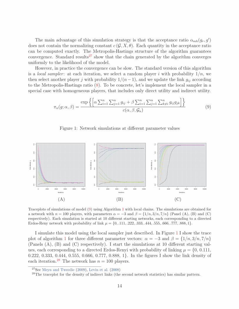
Traceplots of simulations of model (9) using Algorithm 1 with local chains. The simulations are obtained fora network with n = 100 players, with parameters α = −3 and β = {1/n, 3/n, 7/n} (Panel (A), (B) and (C)respectively). Each simulation is started at 10 different starting networks, each corresponding to a directedErdos-Reny network with probability of link μ = {0, .111, .222, .333, .444, .555, .666, .777, .888, 1}.

I simulate this model using the local sampler just described. In Figure 1 I show the traceplot of algorithm 1 for three different parameter vectors: α = −3 and β = {1/n, 3/n, 7/n}(Panels (A), (B) and (C) respectively). I start the simulations at 10 different starting val-ues, each corresponding to a directed Erdos-Renyi with probability of linking μ = {0, 0.111,0.222, 0.333, 0.444, 0.555, 0.666, 0.777, 0.888, 1}. In the figures I show the link density ofeach iteration.28 The network has n = 100 players.

27See Meyn and Tweedie (2009), Levin et al. (2008)28The traceplot for the density of indirect links (the second network statistics) has similar pattern.

14

The simulations (A) with parameters (α, β) = (−3, 1/n) converge to a very sparse net-work; while the simulations (C) with parameters (α, β) = (−3, 7/n) converge to a verydense network. On the other hand, when we consider simulations in (B) with parameters(α, β) = (−3, 3/n), we observe that the chains started at relatively dense networks convergeto a very dense network with density of links μ2 ≈ 0.92, while chains started at relativelysparse networks converge to a sparse network, with link density μ1 ≈ 0.07.

This is a phenomenon that practitioners have encountered in the ERGM literature andin statistical physics models.29 The model seems to put very large probability mass on fewnetworks, an issue called degeneracy. In the next section I provide several theoretical resultsthat explain the such simulation problems.

3.3 Large network analysis

There are two ways to study the asymptotic properties of empirical network formation mod-els. First, we can consider a sample of independent networks and study the properties of themodel as the number of observed networks grows large (many networks asymptotics). Sec-ond, we can consider a single network observation, and a sequence of graphs whose numberof players n grows large (large networks asymptotics). The former case is relatively stan-dard and follows from the theory of exponential families under usual regularity conditions.30

Identification of the parameters is also standard.The case of large networks is relatively more complicated, and only recently gained atten-

tion in the literature.31 It is also the most relevant case in empirical applications, because theeconometrician usually observes a single network in the data.I provide a detailed asymptoticanalysis of the model in the homogeneous players case, using a mix of graph limits theory,large deviations and mean-field approximations for the exponential family.32

Consider a sequence of directed graphs gn, where the number of nodes grows large, n→ ∞. To consider such network limits, I re-scale the potential function, to avoid exploding termsas n→ ∞: each aggregate utility term is scaled by a factor nv(H), where v(H) is the numberof vertices involved in the utility term.

Consider the model

πn(g;α, β) =exp

{n2

[α

∑ni=1

∑nj=1 gij

n2 + β∑n

i=1

∑nj=1

∑nk �=i gijgjk

n3

]}c(α, β,Gn)

(10)

29See Snijders (2002), Butts (2009), Koskinen (2008) for examples.30See Lehman (1983), Sheng (2012), Badev (2013).31See Chandrasekhar and Jackson (2014), Graham (2014), Leung (2014a), DePaula et al. (2014), Ridder

and Sheng (2015), Menzel (2015) for recent contributions.32The explanation that follows is relatively informal, and I leave the technical details about graph limits,

large deviations and mean-field approximations in Appendix D.

15

Notice that the above model is equivalent to the original model (9) with parameter β re-scaledby n.33 Let’s define the re-scaled network statistics

t(H1, g) ≡1

n2

n∑i=1

n∑j=1

gij and t(H2, g) ≡1

n3

n∑i=1

n∑j=1

n∑k �=i

gijgjk

and the corresponding re-scaled potential function T (g)

T (g) = αt(H1, g) + βt(H2, g) (11)

I can then rewrite the model’s likelihood as

πn(g;α, β) =exp {n2 [αt(H1, g) + βt(H2, g)]}

c(α, β,Gn)= exp

{n2 [T (g)− ψn]

}(12)

where the log-normalizing constant ψn is defined as

ψn =1

n2log

∑g∈Gn

exp[n2T (g)

](13)

The following theorems characterize this model as n becomes large, providing an asymptoticapproximation of the normalizing constant and a discussion of identification.34 Theorem2, 3 and 4 below are special cases of a more general result. Indeed, I can show that for alarge class of models, the normalizing constant in (13) solves a variational problem in thespace of probability functions on the unit square (Theorem 10 in Appendix D). Using suchgeneral result I obtain the following theorems.

THEOREM 2 (Non-negative link externalities) Model (10) with non-negative linkexternalities β ≥ 0 exhibits the following behavior for n→ ∞

1. The asymptotic normalizing constant ψ solves

ψ ≡ limn→∞

ψn = maxμ∈[0,1]

{αμ+ βμ2 − μ log μ− (1− μ) log(1− μ)

}(14)

2. The networks generated by the model are indistinguishable from a directed Erdos-Renyigraph with linking probability μ∗, defined as follows:

33This is important when one runs the simulations using the usual ERGM form. For example, one needto use βo = β

n for simulations using the ergm package in the software R. The same is true for the replicationroutines of this paper.

34I use the approach developed in Radin and Yin (2013) and Aristoff and Zhu (2014) to study the maxi-mization problem implied by the simplified variational problem.

16

(a) If the maximization (14) has a unique solution, then μ∗ solves

μ =exp [α + 2βμ]

1 + exp [α + 2βμ](15)

and satisfy 2βμ(1− μ) < 1, for almost all α ∈ R and β ≥ 0.

(b) If the maximization (14) has two solutions, then μ∗ is picked randomly from someprobability distribution over μ∗

1 and μ∗2, such that μ∗

1 < 0.5 < μ∗2 and both solve

equation (15) and satisfy 2βμ(1− μ) < 1.

Proof. See Theorem 11 and Theorem 19 in Appendix D.

The first part of the theorem provides a consistent estimate for the log-normalizing con-stant of model (10), as the solution of a maximization problem. This formulation is theasymptotic analogous of the variational representation of the discrete exponential family inmean parameterization, as shown in Wainwright and Jordan (2008).

The second part of Theorem 2 shows that when β ≥ 0, a realization of the model withparameters (α, β) will be indistinguishable from the realization of a model with parameters(α′, 0) where α′ = log μ∗

1−μ∗ and μ∗ is the maximizer of (14) and solves equation (15). Indeed,both vectors of parameters correspond to the same directed Erdos-Renyi model for largen.35 Moreover, if the maximization problem (14) has two maxima, the parameters (α, β)can generate two completely different networks, one with link density μ∗

1 < 0.5 and one withlink density μ∗

2 > 0.5.36 Such behavior of the model has been observed by practitioners (seeSnijders (2002) for example) using simulation methods, and it was proven analytically forundirected networks in Diaconis and Chatterjee (2011). Our theorem extends their result todirected networks.

There are two main corollaries of Theorem 2: first, the externality cannot be identifiedwhen β ≥ 0; second the network simulation algorithm developed in the ERGM literature anddiscussed in the previous section (ALGORITHM 1) is not necessary for this region of theparameter space. The Erdos-Renyi graphs can be easily simulated using random Bernoullidraws.

On the other hand, when the link externalities are negative and sufficiently large inmagnitude, we can identify the parameters, as shown in the next result.

THEOREM 3 (Negative link externalities) If β < 0 and sufficiently large in magni-tude, the model in (10) is asymptotically different from a directed Erdos-Renyi model.

Proof. See Theorem 14 in Appendix D.

35The model with homogeneous players and only positive externalities violates the condition of expectation-identification in Chandrasekhar and Jackson (2014). The condition requires that different parameters cor-respond to different expected network statistics. This is clearly violated in this special case.

36In the applied mathematics and physics literature, such sets of parameters are crucial because theygenerate a phase transition. See for example Radin and Yin (2013).

17

The problem of asymptotic identification is generated by positive externalities: a modelwith sufficiently large negative externalities generates graphs that do not converge asymp-totically to directed Erdos-Renyi networks. For a sufficiently large negative link externality,model (10) generates networks that are more sparse than an Erdos-Renyi graph. Sparsityindeed has been shown to be an important ingredient for identification in network formationmodels (see Chandrasekhar and Jackson (2014) for example). Furthermore, for β < 0 thelikelihood is unimodal.

Figure 2: Model with negative externalities does not converge to Erdos-Renyi graphs

iterations

links

den

sity

μ

0 2000 4000 6000 8000 10000

0.0

0.2

0.4

0.6

0.8

1.0

iterations

indi

rect

link

s de

nsity

μ

0 2000 4000 6000 8000 10000

0.00

0.05

0.10

0.15

0.20

erdos−renyi μ2

(A) (B)

The 2 panels show simulations of model (10) with parameters (α, β) = (5,−10). The network has n = 300 players, and I run the

simulation for 1500000 iterations, sampling every 150 iterations. In Panel (A) I show the convergence of the direct links density

to μ = 0.3302742. If model (10) converges to an Erdos-Renyi model, then the density of indirect links should be μ2 = 0.109081,

shown as the horizontal dashed line in Panel (B). Therefore the model does not converge to a model with independent links.

The simulations in Figure 2 show evidence that the model with β < 0 does not converge toan Erdos-Renyi model in the large n limit. I use 10 different starting values, corresponding toErdos-Renyi graphs with linking probability μ equi-spaced on the unit interval, for a networkof size n = 300.37 I report simulations for (α, β) = (5,−10), converging to a network densityof μ = 0.3302742 (Figure 2(A)). If the model converges to an Erdos-Renyi graph, the densityof indirect links should be μ2 = 0.109081. Figure 2(B) proves that this is not the case. Indeedour model converges to a different density of indirect links, smaller than the correspondingErdos-Renyi indirect link density.

The results of Theorems 2 and 3 apply to more general models. Consider a model thatincludes the effect of common links, i.e. cyclic triangles, with re-scaled potential

T (g) = αt(H1, g) + βt(H2, g) + γt(H3, g) (16)

37The theoretical results approximate networks of size n > 50 quite well.

18

where the network statistics t(H1, g) and t(H2, g) are the same as in model (10) and t(H3, g) =n−3

∑ni=1

∑nj=1

∑nk �=i gijgjkgki. The following result holds.

THEOREM 4 Consider model (16) as n→ ∞:

1. (Non-negative externalities) If β ≥ 0 and γ ≥ 0, the asymptotic normalizingconstant ψ solves

ψ ≡ limn→∞

ψn = maxμ∈[0,1]

{αμ+ βμ2 + γμ3 − μ log μ− (1− μ) log(1− μ)

}(17)

and the model is asymptotically indistinguishable from a directed Erdos-Renyi graph.The linking probability μ∗ is the maximizer of (17). If the maximization problem (17)has multiple solutions, then μ∗ is picked randomly from some probability distributionover the maximizers.

2. (Negative externalities) If at least one of the externalities is negative (i.e, β < 0or γ < 0) and sufficiently large, then model (16) does not converge asymptotically to adirected Erdos-Renyi graph. In such case, the externalities can be identified.

Proof. These statements are proven in Theorem 12, Theorem 17, Theorem 18 and Theorem16 in Appendix D.

The generalization to additional externalities with alternative utility subgraphs is straight-forward, but tedious. I provide some examples in Appendix D.

The main lesson from this analysis is that models with homogeneous players includingonly positive externalities converge asymptotically to trivial Erdos-Renyi models and areessentially ill-identified in the large n limit. However, as long as at least one externality isnegative and sufficiently large, the model does not degenerate into a trivial independent-linksmodel.

While it was not possible to prove similar results for the more general model with het-erogeneous players, a conjecture is that the sign of the linking externalities is crucial foridentification in these class of models.38

3.4 Convergence of network simulations

The analysis in the previous section shows that in many cases we can approximate thelikelihood of our model using the likelihood of an Erdos-Renyi graph, which is easy toestimate and simulate.

Using similar techniques we can prove that the standard local sampler used in the ERGM

38I am not aware of any result in the literature on graph limits that allows for covariates. Preliminaryresults are contained in Mele and Zhu (2015).

19

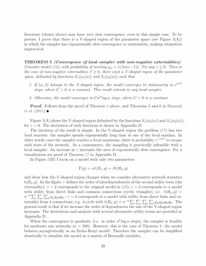
literature (shown above) may have very slow convergence, even in this simple case. To beprecise, I prove that there is a V-shaped region of the parameter space (see Figure 3(A))in which the sampler has exponentially slow convergence to stationarity, making estimationimpractical.

THEOREM 5 (Convergence of local sampler with non-negative externalities)Consider model (16), with probability of meeting ρij = 1/(n(n−1)). Fix any γ ≥ 0. Then inthe case of non-negative externalities β ≥ 0, there exist a V-shaped region of the parameterspace, delimited by functions Sγ(φ1(α)) and Sγ(φ2(α)) such that

1. If (α, β) belongs to the V-shaped region, the model converges to stationarity in eCn2

steps, where C > 0 is a constant. This result extends to any local sampler.

2. Otherwise, the model converges in Cn2 log n steps, where C > 0 is a constant.

Proof. Follows from the proof of Theorem 4 above, and Theorems 5 and 6 in Bhamidiet al. (2011)

Figure 3(A) shows the V-shaped region delimited by the functions Sγ(φ1(α)) and Sγ(φ2(α)),for γ = 0. The derivation of such functions is shown in Appendix D.

The intuition of the result is simple. In the V-shaped region the problem (17) has twolocal maxima: the sampler spends exponentially long time at one of the local maxima. Inother words, once the sampler reaches a local maximum, there is probability e−Cn2

to escapesuch state of the network. As a consequence, the sampling is practically infeasible with alocal sampler. An increase in γ increases the area of exponentially slow convergence. For avisualization see proof of Theorem 17 in Appendix D.

In Figure 3(B) I focus on a model with only two parameters

T (g) = αt(H1, g) + βt(H2, g)

and show how the V-shaped region changes when we consider alternative network statisticst(H2, g). In the figure, r defines the order of interdependencies of the second utility term (theexternality): r = 2 corresponds to the original model in (10); r = 3 corresponds to a modelwith utility from direct links and common connections (cyclic triangles), i.e. t(H2, g) =n−3

∑i

∑j

∑k gijgjkgki ; r = 4 corresponds to a model with utility from direct links and ex-

ternality from 4 connections, e.g. 4-cycle with t(H2, g) = n−4∑

i

∑j

∑k

∑l gijgjkgklgli. The

general result is that if we increase the order of dependencies the size of the V-shaped regionincreases. The derivations and analysis with several alternative utility terms are provided inAppendix D.

When the convergence is quadratic (i.e. in order n2 log n steps), the sampler is feasiblefor moderate size networks (n < 500). However, this is the case of Theorem 4: the modelbehaves asymptotically as an Erdos-Renyi model. Therefore the sampler can be simplifieddrastically to simulate the model as a matrix of Bernoulli variables.

20

Figure 3: Visualization of the regions described in Theorem 5

−20 −10 0 10 20

010

2030

40

α

β

s(φ1(α))

s(φ2(α))

ζ(α)

−20 −10 0 10 200

1020

3040

α

β

r = 2

r = 3

r = 4

(A) (B)

Panel (A) shows the functions Sγ(φ1(α)) and Sγ(φ2(α)) described in Theorem 5. I fix γ = 0 for this picture. The functionζ(α) is the value of the externality β for which problem (17) has two global maxima, for a given parameter α. Panel (B) showshow the V-shaped region delimited by Sγ(φ1(α)) and Sγ(φ2(α)) change if we consider the model with direct utility and onlyone externality, i.e. a model with two parameters only. Here r defines the order of interdependencies of the second utility term(the externality): r = 2 corresponds to the original model in Theorem 2; r = 3 correspond to a model with direct links utilityand utility from common connections (cyclic triangles); r = 4 corresponds to a model with direct links utility and utility from4 common connections (e.g. 4-cycle). If we increase the order of dependencies the size of the region increases. The derivationsand additional utility terms are considered in Appendix D.

In Appendix B, I suggest a modification of the local algorithm that allows for large steps.This should improve convergence when the likelihood is bimodal. I show some simulationevidence that this is the case.

4 Simulation and estimation in finite networks

I estimate the posterior distribution of the structural parameters using an approximateversion of the exchange algorithm (see Murray et al. (2006)). The approximate algorithmuses a double Metropolis-Hastings step to avoid the computation of the normalizing constantc (G, X, θ) in the likelihood, as in Liang (2010).39 Several authors have proposed similar

39This improvement comes with a possible cost: the algorithm may produce MCMC chains of parametersthat have very poor mixing properties (Caimo and Friel, 2010) and high autocorrelation. I partially correctfor this problem by carefully calibrating the proposal distribution. In this paper I use a random walkproposal. Alternatively one could update the parameters in blocks or use recent random block techniques

21

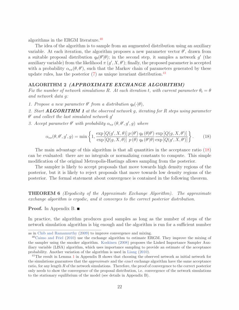
algorithms in the ERGM literature.40

The idea of the algorithm is to sample from an augmented distribution using an auxiliaryvariable. At each iteration, the algorithm proposes a new parameter vector θ′, drawn froma suitable proposal distribution qθ(θ

′|θ); in the second step, it samples a network g′ (theauxiliary variable) from the likelihood π (g′, X, θ′); finally, the proposed parameter is acceptedwith a probability αex(θ, θ

′), such that the Markov chain of parameters generated by theseupdate rules, has the posterior (7) as unique invariant distribution.41

ALGORITHM 2 (APPROXIMATE EXCHANGE ALGORITHM)Fix the number of network simulations R. At each iteration t, with current parameter θt = θand network data g:

1. Propose a new parameter θ′ from a distribution qθ(·|θ),2. Start ALGORITHM 1 at the observed network g, iterating for R steps using parameterθ′ and collect the last simulated network g′

3. Accept parameter θ′ with probability αex (θ, θ′, g′, g) where

αex(θ, θ′, g′, g) = min

{1,

exp [Q(g′, X, θ)]exp [Q(g,X, θ)]

p (θ′)p (θ)

qθ (θ|θ′)qθ (θ′|θ)

exp [Q(g,X, θ′)]exp [Q(g′, X, θ′)]

}. (18)

The main advantage of this algorithm is that all quantities in the acceptance ratio (18)can be evaluated: there are no integrals or normalizing constants to compute. This simplemodification of the original Metropolis-Hastings allows sampling from the posterior.

The sampler is likely to accept proposals that move towards high density regions of theposterior, but it is likely to reject proposals that move towards low density regions of theposterior. The formal statement about convergence is contained in the following theorem.

THEOREM 6 (Ergodicity of the Approximate Exchange Algorithm). The approximateexchange algorithm is ergodic, and it converges to the correct posterior distribution.

Proof. In Appendix B.

In practice, the algorithm produces good samples as long as the number of steps of thenetwork simulation algorithm is big enough and the algorithm is run for a sufficient number

as in Chib and Ramamurthy (2009) to improve convergence and mixing.40Caimo and Friel (2010) use the exchange algorithm to estimate ERGM. They improve the mixing of

the sampler using the snooker algorithm. Koskinen (2008) proposes the Linked Importance Sampler Aux-iliary variable (LISA) algorithm, which uses importance sampling to provide an estimate of the acceptanceprobability. Another variation of the algorithm is used in Liang (2010).

41The result in Lemma 1 in Appendix B shows that choosing the observed network as initial network forthe simulations guarantees that the approximate and the exact exchange algorithm have the same acceptanceratio, for any length R of the network simulations. Therefore, the proof of convergence to the correct posterioronly needs to show the convergence of the proposal distribution, i.e. convergence of the network simulationsto the stationary equilibrium of the model (see details in Appendix B).

22

of iterations.In general, for a fixed number of network simulations R, the samples generated by the

algorithm will converge to a posterior that is ”close” to the correct posterior. As R → ∞the algorithm converges to the exact exchange algorithm of Murray et al. (2006), producingexact samples from the posterior distribution. However, an higher value of R would increasethe computational cost and result in a higher rejection rate for the proposed parameters.

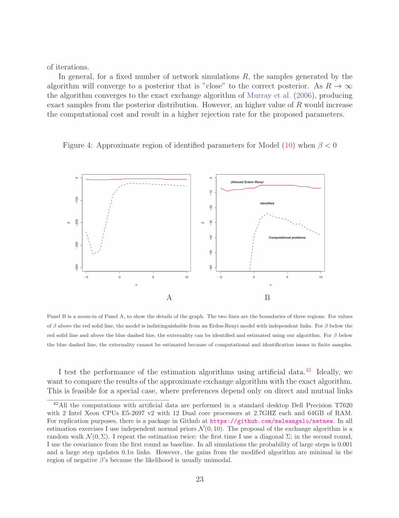
Figure 4: Approximate region of identified parameters for Model (10) when β < 0

−5 0 5 10

−400

−300

−200

−100

0

α

β

−5 0 5 10

−60

−50

−40

−30

−20

−10

0

α

β

(Almost) Erdos−Renyi

Identified

Computational problems

A B

Panel B is a zoom-in of Panel A, to show the details of the graph. The two lines are the boundaries of three regions. For values

of β above the red solid line, the model is indistinguishable from an Erdos-Renyi model with independent links. For β below the

red solid line and above the blue dashed line, the externality can be identified and estimated using our algorithm. For β below

the blue dashed line, the externality cannot be estimated because of computational and identification issues in finite samples.

I test the performance of the estimation algorithms using artificial data.42 Ideally, wewant to compare the results of the approximate exchange algorithm with the exact algorithm.This is feasible for a special case, where preferences depend only on direct and mutual links

42All the computations with artificial data are performed in a standard desktop Dell Precision T7620with 2 Intel Xeon CPUs E5-2697 v2 with 12 Dual core processors at 2.7GHZ each and 64GB of RAM.For replication purposes, there is a package in Github at https://github.com/meleangelo/netnew. In allestimation exercises I use independent normal priors N (0, 10). The proposal of the exchange algorithm is arandom walk N (0,Σ). I repeat the estimation twice: the first time I use a diagonal Σ; in the second round,I use the covariance from the first round as baseline. In all simulations the probability of large steps is 0.001and a large step updates 0.1n links. However, the gains from the modified algorithm are minimal in theregion of negative β’s because the likelihood is usually unimodal.

23

(i.e. excluding friends of friends and popularity effects). These results are in appendix Eand show good performance of the algorithm.

I focus on estimation for the area of parameters that allows identification, i.e. when atleast one of the externalities is negative. The theoretical results suggest that in this regionwe should be able to estimate the externality parameters with precision. I use model (10)to perform the exercise.

The main result is shown in Figure 4(A) (and with more detail in Figure 4(B)). The twolines in the figure delimit three (approximate) regions of the parameters. For values of βabove the solid line, the model is indistinguishable from an Erdos-Renyi model, as in thecase of positive β. Thus the result in Theorem 2 also translates to negative but small β’s.

For β below the solid line and above the dashed line, the parameters are identified. Thisarea correspond to the theoretical result in Theorem 3.

Finally, for values of β below the dashed line, there are some computational problem andestimation becomes impossible: for such values of the externality parameter, the numberof indirect links is too close to zero to allow the network simulation algorithm to provide agood sample.

Figure 5: Example estimates for externality β < 0

●●●●●●●●●●●●●●●●●●●●●●●●●●

●

●

●

●

●

−30 −25 −20 −15 −10 −5 0

−400

−300

−200

−100

010

0

α = 3

true: β

post

. mea

n −

true:

β −

β

●

●

●●●

●●●●

●●

●●●

●●

●●

●●

●

●

●

●

●

●

−30 −25 −20 −15 −10 −5 0

−10

−50

510

α = 3

true: β

post

. mea

n −

true:

β −

β

0 2000 4000 6000 8000 10000

0.00

000.

0002

0.00

040.

0006

0.00

080.

0010

0.00

12

iterations

indi

rect

link

s de

nsity

β = −20β = −25β = −30

A B C

Panel A shows the difference between the true parameter and the estimated posterior mean (red solid line), with 95% credibility

intervals (blue dashed line) for several values of β < 0. Panel B provides closer detail. The estimates are relatively precise when

β > −25. For β ≤ −25 the posterior mean becomes extremely imprecise and the standard deviation of the posterior is huge.

Panel C shows that the problem is the consequence of the simulations hitting lower bound of the network statistics for indirect

links. When β = −25 the simulation output deteriorates so much that estimation becomes impossible.

In Figure 5 I provide a close-up for α = 3. Panel A shows the difference between theestimated posterior mean and the true parameter that generates the data (red solid line)and the 95% credibility interval (blue dashed line). If the estimation is precise we expect thedifference to be close to zero, with small confidence bands. This is the case for most values of

24

the externality β. However, for β < −25 the estimates are so imprecise that the estimationexercise becomes meaningless. This is more evident when we zoom-in the figure in Panel B.The reason for such imprecise estimates is shown in Panel C. When β < −25 the networksimulations hit the lower bound of the indirect links density, i.e. zero. When that happens,the network simulations are extremely inaccurate. In Panel C I show that when β = −20(blue dashed) the MCMC has a regular pattern, while for β = −25 (black dashed) the outputof the sampler is highly irregular and skewed. This creates the computational problems inestimation. I performed the same analysis for a grid of parameters with α ∈ [−5, 10], andβ ∈ [−50, 0]. The results are contained in the replication files.

Figure 6: Approximate region of identified parameters, n = 100 vs n = 200

−5 0 5 10

−800

−600

−400

−200

0

α

β

n=100n=200

−5 0 5 10

−60

−50

−40

−30

−20

−10

0

α

β

n=100n=200

A B

The blue solid line delimits the same regions in Figure 4 for n = 100. The red dashed line delimits the three regions for n = 200.

In Figure 6, I show that the regions where the parameters are identified change with thesize of the network. I compare a model with n = 100 (solid blue lines) to a model withn = 200 players (dashed red lines). The regions are virtually identical for positive values ofα, while they diverge significantly when α < 0.

Finally, in Figure 7 I show the effect of the number of network simulations R on theprecision of the posterior estimates. As an example I report the results for α = 3, but thepattern is the same for other parameters.43 In Panel A and B, I report the difference betweenposterior mean and true β for networks of n = 100 and n = 200 respectively. In Panels Cand D I show the posterior standard deviation.

The estimates with R = 1000 are relatively imprecise and there is almost no precisiongain when we increase networks simulations from R = 10000 to R = 100000.

On the other hand, the cost of increasing the network simulations is almost linear, e.g.

43See the replication files for additional simulations and results.

25

Figure 7: Estimates and length of network simulations

●

●●

●

−30 −25 −20 −15 −10 −5 0

−2−1

01

2

α = 3; n = 100

true: β

post

. mea

n −

true:

β −

β

● R=1000R=10000R=100000

●

●●

●

●−30 −25 −20 −15 −10 −5 0

−2−1

01

2

α = 3; n = 200

true: β

post

. mea

n −

true:

β −

β

● R=1000R=10000R=100000

A B

●

●

●

●

●

−30 −25 −20 −15 −10 −5 0

01

23

45

α = 3; n = 100

true: β

post

. std

. dev

: σβ̂

● R=1000R=10000R=100000

●

●

●

●

●

−30 −25 −20 −15 −10 −5 0

01

23

45

α = 3; n = 200

true: β

post

. std

. dev

: σβ̂

● R=1000R=10000R=100000

C D

computational time increase by 10 times when we increase R from 10000 to 100000. Thuswe conclude that R = 10000 is a good compromise between precision of the estimates andcomputational cost for networks of this size.44

The simulations suggest that convergence is almost quadratic in n in this area of theparameter space. Using the intuition developed in the theoretical result for β ≥ 0, I conjec-ture that the speed of convergence is relatively fast because in this region the likelihood isunimodal.

We conclude that even in the area considered in Theorem 3, where externalities can beidentified, we can encounter estimation problems in finite networks, due to computationalapproximations. In such regions, estimation becomes impossible.

In Appendix B we provide some modification of the local simulation algorithm thatcould improve estimation with multimodal likelihoods, and show some results that accelerateconvergence of the posterior estimation.

44The replication files contain details and estimation times.

26

5 Conclusions

The model presented in this paper shows that an exponential random graph model (ERGM)can be thought of as equilibrium outcome of a strategic network formation game. My modelconsiders payoffs that depend on direct connections but also link externalities, and constrainsthe preferences to guarantee the existence of a potential function. I have shown that suchrestrictions guarantee that the model converges to a unique stationary equilibrium that cor-responds to an ERGM.

I contribute to the literature by studying the equilibrium properties of the model inlarge networks, using a mix of graph limits, large deviations and variational methods forthe exponential family. In particular I show that the sign of the linking externalities iscrucially related to the identification. When the externalities are all positive, the model isasymptotically indistinguishable from an Erdos-Renyi graph. On the other hand, if at leastone of the externalities is negative and sufficiently large, the model does not converge to anErdos-Renyi graph and the externality can be identified.

I propose a Bayesian MCMC estimation method using an approximate exchange algo-rithm. Our theoretical identification result shows that negative and sufficiently large exter-nalities can be estimated and identified. However, I show that in finite networks there aresome computational problems even in this region of the parameter space, making estimationof the link externalities infeasible in some cases.

In this paper, I have considered approximate estimation through sampling, using aMarkov Chain Monte Carlo method to approximate the likelihood and the posterior dis-tribution of the parameters. As an alternative, we could approximate the likelihood usinga variational deterministic technique. Some preliminary attempts in this direction are pro-vided in He and Zheng (2013) and Mele (2015), using (structural) mean-field approximationsfor the exponential family (see Wainwright and Jordan (2008) and Bishop (2006)). An al-ternative approach is provided in Chandrasekhar and Jackson (2014), by imposing sparsity,which implies good statistical properties of the estimators and improves the tractability ofthe model.

In the development of a model of empirical network formation, we also need to considerhow modeling unobserved heterogeneity affects our results. Graham (2014) includes unob-served heterogeneity in a model with heterogeneous agents, but excludes the link externalitiesthat are central to the model presented here. I can include unobserved heterogeneity in ourmodel, with substantial increase in computational burden. However, it is not clear that wecan separately identify externalities and unobserved heterogeneity using only one networkrealization.

References

Acemoglu, D., M. Dahleh, I. Lobel and A. Ozdaglar (2011), ‘Bayesian learning in socialnetworks’, Review of Economic Studies forthcoming.

27

Amemiya, Takeshi (1981), ‘Qualitative response models: A survey’, Journal of EconomicLiterature 19(4), 1483–1536.

Andrieu, C. and G. O. Roberts (2009), ‘The pseudo-marginal approach for efficient montecarlo computations’, Annals of Statistics 37(2), 697–725.

Aristoff, David and Lingjiong Zhu (2014), On the phase transition curve in a directed expo-nential random graph model.

Atchade, Yves and Jing Wang (forthcoming), ‘Bayesian inference of exponential randomgraph models for large social networks’, Communications in Statistics - Simulation andComputation .

Athey, Susan and Guido Imbens (2007), ‘Discrete choice models with multiple unobservedchoice characteristics’, International Economic Review 48(4), 1159–1192.

Badev, Anton (2013), Discrete games in endogenous networks: Theory and policy.

Bala, Venkatesh and Sanjeev Goyal (2000), ‘A noncooperative model of network formation’,Econometrica 68(5), 1181–1229.

Bandiera, Oriana and Imran Rasul (2006), ‘Social networks and technology adoption innorthern mozambique’, Economic Journal 116(514), 869–902.

Besag, Julian (1974), ‘Spatial interaction and the statistical analysis od lattice systems’,Journal of the Royal Statistical Society Series B (Methodological) 36(2), 192–236.

Bhamidi, Shankar, Guy Bresler and Allan Sly (2011), ‘Mixing time of exponential randomgraphs’, The Annals of Applied Probability 21(6), 2146–2170.

Bishop, Christopher (2006), Pattern recognition and machine learning, Springer, New York.

Blume, Lawrence E. (1993), ‘The statistical mechanics of strategic interaction’, Games andEconomic Behavior 5(3), 387–424.

Boeckner, Derek (2013), Directed graph limits and directed threshold graphs. PhD Thesis.

Borgs, C., J.T. Chayes, L. Lovsz, V.T. Ss and K. Vesztergombi (2008), ‘Convergent se-quences of dense graphs i: Subgraph frequencies, metric properties and testing’, Advancesin Mathematics 219(6), 1801 – 1851.

Boucher, Vincent (2013), Structural homophily.

Butts, Carter (2009), Using potential games to parameterize erg models. working paper.

Caimo, Alberto and Nial Friel (2010), ‘Bayesian inference for exponential random graphmodels’, Social Networks forthcoming.

28

Chandrasekhar, Arun and Matthew Jackson (2014), Tractable and consistent exponentialrandom graph models.

Chatterjee, Sourav and Amir Dembo (2015), Nonlinear large deviations, Working papers,Stanford University.

Chatterjee, Sourav and S.R.S. Varadhan (2011), ‘The large deviation principle for the erdos-rnyi random graph’, European Journal of Combinatorics 32(7), 1000 – 1017. Homomor-phisms and Limits.URL: http://www.sciencedirect.com/science/article/pii/S0195669811000655

Chib, Siddartha and Srikanth Ramamurthy (2009), ‘Tailored random block’, Journal ofEconometrics .

Christakis, Nicholas, James Fowler, Guido W. Imbens and Karthik Kalyanaraman (2010),An empirical model for strategic network formation. Harvard University.

Conley, Timothy and Christopher Udry (forthcoming), ‘Learning about a new technology:Pineapple in ghana’, American Economic Review .

Cooley, Jane (2010), Desegregation and the achievement gap: Do diverse peers help? workingpaper.

Currarini, Sergio, Matthew O. Jackson and Paolo Pin (2009), ‘An economic model of friend-ship: Homophily, minorities, and segregation’, Econometrica 77(4), 1003–1045.

Currarini, Sergio, Matthew O. Jackson and Paolo Pin (2010), ‘Identifying the roles of race-based choice and chance in high school friendship network formation’, the Proceedings ofthe National Academy of Sciences 107(11), 48574861.

De Giorgi, Giacomo, Michele Pellizzari and Silvia Redaelli (2010), ‘Identification of socialinteractions through partially overlapping peer groups’, American Economic Journal: Ap-plied Economics 2(2).

De Marti, Joan and Yves Zenou (2009), Ethnic identity and social distance in friendshipformation, Cepr discussion papers, C.E.P.R. Discussion Papers.

DePaula, Aureo, Seth Richards-Shubik and Elie Tamer (2014), Identification of preferencesin network formation games. working paper.

Diaconis, Persi and D. Stroock (1991), ‘Geometric bounds for eigenvalues of markov chains’,Annals of Applied Probability 1(1), 36–61.

Diaconis, Persi and Sourav Chatterjee (2011), Estimating and understanding exponentialrandom graph models.

29

Echenique, Federico, Roland G. Fryer and Alex Kaufman (2006), ‘Is school segregation goodor bad?’, American Economic Review 96(2), 265–269.

Frank, Ove and David Strauss (1986), ‘Markov graphs’, Journal of the American StatisticalAssociation 81, 832–842.

Gelman, A., G. O. Roberts and W. R. Gilks (1996), ‘Efficient metropolis jumping rules’,Bayesian Statistics 5, 599–608.

Gelman, A., J. Carlin, H. Stern and D. Rubin (2003), Bayesian Data Analysis, SecondEdition, Chapman & Hall/CRC.

Gilles, Robert P. and Sudipta Sarangi (2004), Social network formation with consent, Dis-cussion paper, Tilburg University, Center for Economic Research.

Goldsmith-Pinkham, Paul and Guido W. Imbens (2013), ‘Social networks and the identifi-cation of peer effects’, Journal of Business and Economic Statistics 31(3), 253–264.

Golub, Benjamin and Matthew Jackson (2011), ‘Network structure and the speed of learning:Measuring homophily based on its consequences’, Annals of Economics and Statistics .

Graham, Bryan (2014), An empirical model of network formation: detecting homophily whenagents are heterogeneous. working paper.

He, Ran and Tian Zheng (2013), Estimation of exponential random graph models for largesocial networks via graph limits, in ‘Proceedings of the 2013 IEEE/ACM InternationalConference on Advances in Social Networks Analysis and Mining’, ASONAM ’13, ACM,New York, NY, USA, pp. 248–255.

Heckman, James J. (1978), ‘Dummy endogenous variables in a simultaneous equation sys-tem’, Econometrica 46(4), 931–959.

Hsieh, Chih-Sheng and Lung-Fei Lee (2012), A structural modeling approach for networkformation and social interactions with applications to students’ friendship choices andselectivity on activities.

Jackson, Matthew and Alison Watts (2001), ‘The existence of pairwise stable networks’,Seoul Journal of Economics 14(3), 299–321.

Jackson, Matthew and Allison Watts (2002), ‘The evolution of social and economic networks’,Journal of Economic Theory 106(2), 265–295.

Jackson, Matthew and Asher Wolinsky (1996), ‘A strategic model of social and economicnetworks’, Journal of Economic Theory 71(1), 44–74.

Jackson, Matthew O. (2008), Social and Economics Networks, Princeton.

30

Koskinen, Johan H. (2008), The linked importance sampler auxiliary variable metropolishastings algorithm for distributions with intractable normalising constants. MelNet So-cial Networks Laboratory Technical Report 08-01, Department of Psychology, School ofBehavioural Science, University of Melbourne, Australia.

Laschever, Ron (2009), The doughboys network: Social interactions and labor market out-comes of world war i veterans. working paper.

Lehman, E. L. (1983), Theory of Point Estimation, Wiley and Sons.

Leung, Michael (2014a), A random-field approach to inference in large models of networkformation. working paper.

Leung, Michael (2014b), Two-step estimation of network-formation models with incompleteinformation. working paper.

Levin, David. A, Yuval Peres and Elizabeth L. Wilmer (2008), Markov Chains and MixingTimes, American Mathematical Society.

Liang, Faming (2010), ‘A double metropolis-hastings sampler for spatial models with in-tractable normalizing constants’, Journal of Statistical Computing and Simulation forth-coming.

Liang, Faming, Chuanhai Liu and Raymond J. Carroll (2010), Advanced Markov ChainMonte Carlo Methods: Learning from Past Samples, John Wiley and Sons, Ltd.

Lovasz, L. (2012), Large Networks and Graph Limits, American Mathematical Society col-loquium publications, American Mathematical Society.

Lovasz, Laszlo and Balazs Szegedy (2007), ‘Szemeredi’s lemma for the analyst’, GAFA Ge-ometric And Functional Analysis 17(1), 252–270.

Mele, Angelo (2015), Approximate variational inference for a model of social interactions.Working Paper.

Mele, Angelo and Lingjiong Zhu (2015), Variational approximations for large strategic ergms.

Menzel, Konrad (2015), Strategic network formation with many agents, Working papers,NYU.

Meyn, Sean and Richard L. Tweedie (2009), Markov Chains and Stochastic Stability, Cam-bridge University Press.

Miyauchi, Yuhei (2012), Structural estimation of a pairwise stable network formation withnonnegative externality.

Monderer, Dov and Lloyd Shapley (1996), ‘Potential games’, Games and Economic Behavior14, 124–143.

31

Murray, Iain A., Zoubin Ghahramani and David J. C. MacKay (2006), ‘Mcmc for doubly-intractable distributions’, Uncertainty in Artificial Intelligence .

Nakajima, Ryo (2007), ‘Measuring peer effects on youth smoking behavior’, Review of Eco-nomic Studies 74(3), 897–935.

Radin, Charles and Mei Yin (2013), ‘Phase transitions in exponential random graphs’, TheAnnals of Applied Probability 23(6), 2458–2471.

Ridder, Geert and Shuyang Sheng (2015), Estimation of large network formation games,Working papers, UCLA.

Robert, Christian P. and George Casella (2005), Monte Carlo Statistical Methods (SpringerTexts in Statistics), Springer-Verlag New York, Inc., Secaucus, NJ, USA.

Rossi, P., R. McCulloch and G. Allenby (1996), ‘The value of purchase history data in targetmarketing’, Marketing Science 15(4), 321–340.

Sheng, Shuyang (2012), Identification and estimation of network formation games.

Snijders, Tom A.B (2002), ‘Markov chain monte carlo estimation of exponential randomgraph models’, Journal of Social Structure 3(2).

Tamer, Elie (2003), ‘Incomplete simultaneous discrete response model with multiple equilib-ria’, The Review of Economic Studies 70(1), 147–165.

Topa, Giorgio (2001), ‘Social interactions, local spillovers and unemployment’, Review ofEconomic Studies 68(2), 261–295.

Wainwright, M.J. and M.l. Jordan (2008), ‘Graphical models, exponential families, andvariational inference’, Foundations and Trends@ in Machine Learning 1(1-2), 1–305.

Wasserman, Stanley and Philippa Pattison (1996), ‘Logit models and logistic regressions forsocial networks: I. an introduction to markov graphs and p*’, Psychometrika 61(3), 401–425.

32