A Strength Theory for Free Recall - Queen's U
119
A Strength Theory for Free Recall by Donald R. J. Franklin A thesis submitted to the Department of Psychology in conformance with the requirements for the degree of Doctor of Philosophy Queen’s University Kingston, Ontario, Canada January, 2013 Copyright © Donald R. J. Franklin, 2012
Transcript of A Strength Theory for Free Recall - Queen's U

A Strength Theory for Free Recall
by
Donald R. J. Franklin
A thesis submitted to the Department of Psychology
in conformance with the requirements for
the degree of Doctor of Philosophy
Queen’s University
Kingston, Ontario, Canada
January, 2013
Copyright © Donald R. J. Franklin, 2012

ii
Abstract
A model for free recall of words is presented and applied to representative free-recall
experiments. According to the model, a subject's lexicon contains a representation for
each word and for the association between each pair of words. Studying a word in a list
strengthens that word's representation in the lexicon, but reduces the strength of
previously studied words. In addition, while studying the list, the subject associates pairs
of items and, thereby, strengthens the corresponding associations in the lexicon. A
subject's efficiency at forming associations drops off as the number of pairs increases.
Retrieval is initiated with a report cue. Selection of an item for report is based on its
strength in the lexicon plus the strength of its association with the retrieval cue. Selecting
an item for report changes the strength of its association with the cue in the lexicon. To
test the model, parameters were obtained by fitting it to serial-position curves taken from
the archival literature. The model predicted three additional dependent measures: order of
report, items correct per trial, and the number of intrusions per trial. In addition, I applied
the model to phenomena associated with the free-recall task and showed that it captures
the list-strength effect, interference in part-list cuing, clustering with categorized lists,
and distraction effects. The model itself does not change to capture these experimental
data. Word lists are presented to the model according to the experimental protocol used in
the original experiments, and the model captures output measures derived from the
experimental data. The model demonstrates that simple mechanisms can capture a wide
range of apparently complex behaviour if we allow for a large enough knowledge base.
In effect, the complexity of behaviour in free-recall paradigms lies in the interactions in
the lexicon, not in the complexity of the recall mechanisms.

iii
Acknowledgements
I would like to thank my supervisor, Doug Mewhort, for the assistance given
throughout the development and testing of this model. Doug is a hard taskmaster with
very high standards. He has a comprehensive set of modeling skills and an excellent
understanding of the memory literature. He is ready and willing to pass on his knowledge
to those interested. Doug takes a keen interest in the work of his graduate students and is
prepared to discuss/argue theory at any time. His sense of humour helps to smooth over
any criticisms he may feel obliged to point out. All in all, he is an ideal advisor.
I would also like to thank Dr. E. E. Johns for providing me with sources of
information. Beth is a gifted empiricist who constantly reinforces an understanding that
the goal of modeling is to present predictions that can be verified or refuted empirically,
and to expand theory.
Ben Murdock of the University of Toronto was kind enough to share original data
files with me for experiments of his used in this paper. Ben was very supportive of my
efforts. This encouraged me, for he has always been one of my heroes in the field of
memory study.
Thanks to Mike Jones, Randy Jamieson and to Vlad Zotov for patiently listening
to me talk about my research, even though their own work had to be uppermost in their
mind all the while. Our exchanges have been often fruitful and exciting.
Finally, I want to thank my examining committee, Professors Rick Beninger,
Ingrid Johnsrude, Dorthea Blostein (Queen`s), and Bill Hockley (Wilfrid Laurier).

iv
Table of Contents
Abstract ………………………………………………………………………………….. ii
Acknowledgements …………………………………………………………………….. iii
Table of Contents ……………………………………………………………………….. iv
List of Figures ………………………………………………………………………….. vii
Chapter 1: Introduction……………………………………………………………………1
Chapter 2: An examination of some models of memory ………………………………... 5
The Modal Model ……………………………………………………………….. 5
An Instantiation of the Modal Model …………………………………………… 6
Critique of the Modal Model ……………………………………………………. 6
Associative Chaining Models……………………………………………………10
The Theory of Distributed Associative Memory (TODAM)…………….11
Changing Context Based Theories …………………………………………….. 13
The Perturbation Model ………………………………………………... 13
The Positional Distinctiveness Model …………………………………. 14
Oscillator-Based Memory for Serial Order (OSCAR) ………………… 14
The Temporal Context Model………………………………………….. 15
The Primacy Model…………………………………………………….. 17
Chapter 3: A Strength Theory for Recall ………………………………………………. 19
Chapter 4: Implementing the Theory: A Model for Free Recall ………………………. 23
Representing items and associations ……………………………………….... 23
Studying the List …………………………………………………………...….26
Retrieving Items from Memory ………………………………………………. 28

v
A sample trial …………………………………………………………………... 31
Chapter 5: Applying the Model ………………………………………………………... 33
Immediate Free Recall: Basic Data ……………………………………………. 33
Prediction across list length ……………………………………………………. 39
Evaluating the Model: Other Free-Recall Paradigms ………………………….. 46
Distraction paradigms ………………………………………………….. 46
The list-strength effect …………………………………………………. 57
Part-list cuing ………………………………………………………….. 60
Categorized lists ………………………………………………………... 66
Chapter 6: Mistaken Assumptions in Scoring Order of Report………………………….73
Chapter 7: Limitations of the Model…………………………………………………….77
Chapter 8: An Updated Model …………………………………………………………. 81
Chapter 9: Discussion ………………………………………………………………….. 89
References ……………………………………………………………………………… 96
Appendix A: Linear Convolution Explained …………………………………………..106
Appendix B: Linear Correlation Explained ……………………………………………107
Appendix C: Circular Convolution Explained …………………………………………108
Appendix D: Circular Correlation Explained ………………………………………….109
Appendix E: Fixed Parameters Used in the Simulations ……………………..………..110
Appendix F: Free Parameters Used in the Simulations………………………………...111
Appendix G: Parameters Used in the Updated Model Simulation……………………..112

vi
List of Figures
Figure 1: The Modal Model ………………………………………………………...…… 5
Figure 2: The conception of memory expressed by Cowan (1988) …………………....... 7
Figure 3: Data estimated from Rundus & Atkinson (1970) and geometric fit to curve... 28
Figure 4: Momentary strength for a sample trial ………………………………………. 32
Figure 5: Murdock and Okada (1970) Serial Position Curve ………………………….. 34
Figure 6: Murdock and Okada (1970) Words Correct per Trial ……………………….. 36
Figure 7: Murdock and Okada (1970) Cumulative Frequency of Kendall’s τ…………. 37
Figure 8: Murdock and Okada (1970) Intrusions ……………………………………… 38
Figure 9: Murdock (1962) twenty and thirty-item lists presented at 1 word per second. 41
Figure 10: Murdock (1962) twenty and fifteen-item lists at 2 words per second …….... 42
Figure 11: Strength of representation for item and associative information …………... 44
Figure 12: The sum of item and associative strengths by position, rate, and list-length ..45
Figure 13: Percent correct as a function of position and end-of-list distraction ……….. 50
Figure 14: Percent correct by presentation position and distraction condition ………… 53
Figure 15: Item and associative strengths in simulating Koppenaal and Glanzer (1990) 56
Figure 16: Tulving and Hastie (1972), Experiment 1 ………………………………….. 58
Figure 17: Slamecka (1968): Recall as a function cue type and scoring criterion……... 63
Figure 18: Percent correct recall of non-cued items as a function of the type of cue ….. 65
Figure 19: Dallet (1964) ………………………………………………………………... 70
Figure 20: OPC curves for groups of ten trials in ascending order ……………………. 74
Figure 21: CRP curves for groups of ten trials in ascending order ……………………. 75

vii
Figure 22: Words recalled per trial for the four ten-trial blocks in Figures 19 and 20… 76
Figure 23: OPC curves for groups of ten trials in ascending order ……………………. 77
Figure 24: CRP curves for groups of ten trials in ascending order ……………………. 77
Figure 25: OPC and CRP curves for groups of trials [Murdock & Okada (1970) slow]. 78
Figure 26: OPC and CRP curves for groups of trials [Murdock & Okada (1970) fast]... 79
Figure 27: OPC curves Roberts (1972) 20 item lists …………………………………... 80
Figure 28: Updated Model: SP curve [Murdock (1962) twenty items at 1 per second]... 84
Figure 29: Updated Model: cumulative distribution of words correct per trial …………85
Figure 30: Updated Model: CRP curves first ten trials of Murdock (1962) …………….86
Figure 31: Updated Model: OPC curve of the first 10 trials of Murcock (1962) ……….87

1
Chapter 1: Introduction
Biological memory cannot be seen, touched or felt. It is inferred from behavior. The
ethereal quality of memory makes it difficult to study. In 1885, Hermann
Ebbinghaus demonstrated one way to study declarative memory experimentally.
Ebbinghaus studied lists of items (words) and then attempted to recall as many of
the list items as possible. In some experiments, he attempted to recall the items in
the same order in which he had studied them (Serial Recall). In other experiments,
he tried to recall as many items as possible, without regard to order (Free Recall). I
use the term memory throughout this paper to refer to declarative memory.
Declarative memory allows remembered material to
be compared and contrasted. The stored
representations are flexible, accessible to awareness,
and can guide performance in a variety of contexts.
Declarative memory is representational. It provides a
way of modeling the external world, and it is either
true or false. (Squire & Wixted, 2011)
List-learning experiments have remained one of the main tools used to study
memory. Ebbinghaus (1885) used letter trigrams in his experiments in an attempt to
eliminate any role for prior experience with the stimuli. Later researchers came to
realize that the sound of trigrams mimicked the sound of word parts, or, in some
cases, whole words, and so prior experience with them could not be ruled out. The
majority of list-learning experiments since have used words as list items. Memory
theory has been primarily built around the results of such experiments.

2
Ebbinghaus was quick to discover that all items in a list did not have an
equal probability of being recalled. Beginning items have a higher probability of
recall, as do the last few list items. Plotting proportion recalled for each serial
position in the list typically produces a U-shaped Serial Position Curve (SPC). The
higher values of recall for the items at the beginning of the list is now known as the
primacy effect, since these were the first presented items. The higher values for
recall of items at the end of the list is called the recency effect, since those items
were the most recently presented.
Ebbinghaus also spoke of a forgetting curve, the complement of the SPC.
There are several possibilities for why we forget. It could be that the item is no
longer in memory: a storage-failure explanation. It is possible that the item is still in
memory, but that it can’t be retrieved: a retrieval-failure explanation. Both
explanations have had their adherents: Gold and King (1974) advocate for storage
failure, while Miller and Springer (1973) support a retrieval failure interpretation.
Tulving and Pearlstone (1966) demonstrated experimentally that, if proper
cues to recall were given to subjects, the number of words recalled was greater than
for uncued recall. The result shows that items may be present in memory but not
accessible for report. Perhaps the cues strengthened item representation in memory,
allowing for recall of items so strengthened. Such a result supports a retrieval
failure explanation. Wickelgren and Norman (1966) proposed a strength theory of
memory and tested several strength-based models, all of which presumed a two-
store store account of memory. That is, a memory system with separate short-term
and long-term stores.

3
This thesis presents a strength theory of memory. I propose that the strength
of word representations in our lexicon determines both what is reported and the
order in which it is reported. The theory presents a single-store account of memory
that is formalized in a mathematical model. The model is used to test the limitations
of the theory I present. In essence, I wish to examine how far a strength theory
using a single memory store can take us in accounting for the results of list-learning
experiments.
The model is tested by fitting one aspect of human recall data, the SPC. The
data the model is fitted to is drawn from the simple Free-Recall paradigm. In the
Free-Recall paradigm, a cue that list presentation is about to begin is first presented.
Following the cue, the participant is presented with a list of items, usually words.
The time between successive words (the inter-stimulus interval) is held constant.
After the last list item has been presented, the participant receives a cue to begin
recall, and the time between the last item presented and the recall cue is controlled.
The participant is free to recall the list in any order they choose. The unconstrained
nature of recall in this paradigm allows for an excellent window into memory
organization, storage, and retrieval.
I will show that the model captures the data to which it has been fitted. In
doing so, it also captures other aspects of performance in the experimental data to
which it has not been fitted. I will also show that the model captures effects
introduced by manipulating the simple Free-Recall paradigm. Manipulations
include changing the inter-stimulus interval; changing list length; repeating some
items; delaying recall after presenting the last list item, and having the participant

4
perform an interpolated task during the delay interval; delaying the presentation of
each word by using a filled delay interval. All of the aforementioned manipulations
on the standard free-recall paradigm have strongly affected memory theory. The
model requires no alterations to capture these manipulations.
I present no original experimental work in this paper. There is a vast amount
of archival data available to me. Every time the model successfully accounts for one
of the manipulations on the standard free recall paradigm gives support to the
theoretical principles that it is founded upon. In effect, every run of the model can
be considered an experiment testing the theory that the model is based upon. And
so, I present you with the results of many experimental tests of my theory.

5
Chapter 2: An Examination of Some Models of Memory
The Modal Model
For over forty years the modal model of memory (Atkinson & Shiffrin,
1968; Waugh & Norman, 1965) has been the dominant theory of memory storage
and retrieval. Atkinson and Shiffrin (1968) give the most complete account of this
theory. Figure 1 presents Atkinson & Shiffrin’s theory diagrammatically. They
posited two separate memory stores existing in the brain. Information flows into a
limited capacity Short-Term Memory (STM). Rehearsal operations occur in STM.
Once the capacity of STM is reached, each new incoming item causes an item to be
dropped from STM. Associations between items are formed in STM. The strength
of association between any two items is determined by the length of time they
spend together in the short-term store. If an item stays in STM long enough, it and
its associative information pass into Long-Term Memory (LTM). During retrieval,
the items in STM are first dumped, and then LTM associations are probed in an
attempt to retrieve more items.
Figure 1. A diagram of the Atkinson and Shiffrin Model showing the two memory stores,
information flow between stores, and the operations which occur in each store.
The Modal Model was given strong support by Rundus and Atkinson
(1970), who had subjects rehearse overtly. The number of rehearsals given an item
STMRehearsal
Retrieval Forgetting
LTM

6
was high for those items presented near the beginning of the list (primacy), but
dropped off for items in the middle. Rundus and Atkinson attributed the primacy
effect to the first few items being well represented in LTM, due to a longer time
spent in the rehearsal buffer.
An Instantiation of the Modal Model
Raaijmakers and Shiffrin (1981, 1982) presented the Search of Associative
Memory (SAM) model. SAM is a formalized version of the Modal Model. It adds
one thing to the model of Atkinson and Shiffrin (1968). Not only are item-to-item
associations created in short-term store, but item-to-list context associations are also
created. Unlike many other models using context, in SAM, list context does not
vary over time. SAM represents LTM as a store of item-to-item and cue-to-item
associative weights.
In retrieval, context is used as a cue until an item is recovered. Then context
and the recovered item are used together as a cue. If retrieval fails a set number of
times, search reverts to context only. If context cueing fails a set number of times,
retrieval stops. SAM makes no assumptions about how items are stored in memory.
Without representation assumptions, SAM is incapable of reproducing interactions
between items and between associations stored in memory during memorization
and retrieval.
Critique of the Modal Model
In seeking to compartmentalize cognitive functioning, the modal model
reflects the ‘brain as a computer’ thinking of its era. Such modular thinking has had
a history of detractors. As long ago as 1902, Loeb expressed the opinion that “in

7
processes of association the cerebral hemispheres act as a whole, and not as a
mosaic of a number of independent parts.” There is a growing body of opinion
drawn from disparate sources expressing doubt about localizing memory one
distinct compartment in the brain.
We now have reason to believe that long-term memory is stored in
the cerebral cortex. Moreover, it is stored in the same area of the
cerebral cortex that originally processed the information—that is,
memories of visual images are stored in various areas of the visual
cortex, and memories of tactile experiences are stored in the
somatosensory cortex. Kandel (2006, p. 80)
Cowan (1988) conceives of memory as a hierarchy. STM is the activated
portion of LTM. Within STM, attention focuses on a subset of items. Figure 2
diagrams the conception of memory expressed by Cowan (1988, 1993).
Figure 2. The conception of memory expressed by Cowan (1988). STM is shown as an activated
subset of LTM. Within STM some items receive greater attention.
LTM
S TM
Focus of Attention

8
Cowan’s ideas are given support by Ruchkin, Grafman, Camero, and Berndt (2003,
p. 711) who state “the neuropsychological evidence for distinct short-term and
long-term memory stores is not compelling.”
Eric Kandel, who received the Nobel Prize for a lifetime of work focusing
on the neurobiology of memory, provides us biological data that support Cowan’s
conception of memory.
Consistent with the one-process theory, the same site can give rise to
both short-term and long-term memory… Moreover, in each case a
change in synaptic strength occurs. But consistent with the two-
process theory, the mechanisms of short and long-term change are
fundamentally different. Short-term memory produces a change in
the function of the synapse, strengthening or weakening preexisting
connections; long-term memory requires anatomical changes.
Repeated sensitization training (practice) causes neurons to grow
new terminals, giving rise to long-term memory. (Kandel, 2006, p.
126).
Working memory (WM) was initially defined as something different from
STM. WM was thought to use STM to briefly store information pertinent to some
task at hand. There has been a trend in the literature to use WM and STM
interchangeably. I am of the opinion that, in the free-recall task, subjects are using
WM, after all, they are being asked to perform a task. What is labeled as STM in
Cowan’s model might better be called working memory. I would also use the terms
interchangeably.

9
Bjork and Whitten (1974) performed a number of experiments in which
distraction activity was administered before and after presentation of each word pair
in a list. Subjects were required to study only those word pairs just presented.
According to the Modal Model, the distraction activity should have nullified the
recency effect in recall entirely. Primacy should also have been cancelled out by the
requirement to study only the items just presented. Contrary to Modal Model
predictions, the SPC’s for immediate recall showed marked primacy and recency
effects. Among their conclusions, Bjork and Whitten stated “The customary two-
process theoretical account of immediate free recall is certainly incomplete, if not
wrong” (p. 189).
Craik and Lockhart (1972) gave convincing arguments for a Levels
of Processing theory. They were of the view that material could be analysed
at different levels. Depth of analysis is dependent on several factors. If the
material is meaningful, it can be analysed at a deeper cognitive level than
meaningless material. Longer processing time allows for deeper processing.
The nature of the orienting task is important. If the orienting task allows for
only shallow processing, we get the standard limited capacity effects that are
used to support the two-store theory. An orienting task that promotes deeper
processing does not show such limited capacity. They draw convincing
arguments from the literature to support their theory. In their conclusions,
Craik and Lockhart state ``While multistore models have played a useful
role, we suggest that they are often taken too literally`` (p. 681). For more

10
criticism of the Modal Model, see Baddeley & Hitch (1977), Bjork &
Whitten (1974), Whitten & Bjork, (1972, 1977), and Wickelgren (1970).
I am of the view that there is already a long-term store of word
representations at our disposal, the lexicon. There is no need to ‘encode’ a word in
some temporary store and then pass it along to the lexical store. Such thinking
disregards participants’ prior knowledge. I theorize that representations of particular
words stored in the lexicon could be strengthened when those particular words are
heard, or read. Recalling a word should also increase the strength of its
representation. Strengthening a word’s representation should have interactive
repercussions on all lexical entries, strengthening some and weakening others. In
effect, the lexicon is a dynamic system, where word strengths are constantly
changing according to environmental and internal stimuli. Ebbinghaus (1885) was
trying to escape lexical interactions by using nonsense syllables.
Associative-Chaining Models
That associations between events are crucial to recall is an ancient premise.
In his De Memoria et Reminiscentia, Aristotle (384-322 B.C) proposed that events
contiguous in time or space become associated. Hebart (1824) formulated a
mathematical theory in which links between contiguous events are axiomatic (for a
summary see Boudewinjnse, Murray, & Bandomir, 1999, 2001). For behaviorists,
association is the sine qua non of learning. The behaviorist approach dominated
psychology from the early part of the twentieth century until the cognitive
revolution of the 1960’s. Behaviourist methods are still used today to treat phobias

11
and compulsive behaviours. Neurobiological evidence exists showing that
associations between stimuli can be formed in the brain.
Aristotle, and subsequently the British empiricist
philosophers and many other thinkers, had proposed that learning
and memory are somehow the result of mind's ability to associate
and form some lasting mental connection between two ideas or
stimuli. With the discovery of the NMDA receptor and longterm
potentiation, neuro-scientists had unearthed a molecular and cellular
process that could well carry out this associative process. (Kandel,
2006 p. 166).
According to associative-chaining models of recall, we store information
about items and associations between overlapping pairs of items. In such accounts,
chaining is analogous to the behaviorist’s S-R account of animals learning a maze.
To recall, chaining models typically suppose that participants follow the associative
chain so that each recalled item acts as the probe (stimulus) leading to recall of the
next item in the chain. All chaining models share a common problem. If no item is
recovered on a particular retrieval attempt, how does recall proceed beyond that
point without a new probe? In effect, by postulating that retrieval runs down the
associative chain, chaining models stall too early in recall.
The Theory of Distributed Associative Memory (TODAM)
Murdock’s (1982) theory of distributed associative memory (TODAM) is a
classic example of a chaining model. In TODAM, an item, I, is represented by a
vector of N components. Components are designated as features, fi, that describe the

12
item. Feature values are centred on index zero. Each feature value is assigned by
sampling from a Gaussian distribution with mean of zero and variance of 1/ N.
I = …0, 0, f-a, f-(a-1), … f0 , …, f(a-1), , fa, 0, 0, …
where a = (N-1)/2.
Vectors constructed in this manner have valuable characteristics. The Euclidean
inner product (dot product) of a vector with any other vector has an expected value
of zero, while the dot product of a vector with itself has an expected value of one.
Ε[Ii ● Ij] = 0.0
Ε[Ii ● Ii] = 1.0
The association of two vectors is formed by linear convolution. Linear
convolution is described in Appendix A. The symbol for linear convolution is *. We
have, therefore, the following equation for associating two vectors, Ii and Ij:
A = (Ii * Ij),
where A is the association of Ii and Ij. Convolution is bidirectional, that is, (Ii * Ij)
= (Ij * Ii).
In TODAM, linear correlation, designated by the symbol #, is used in
retrieval.
If A = (Ii * Ij), then (Ii # A) = Ijʹ and Ijʹ is similar to Ij as measured by the
dot product.
Ε[Ij ● Ijʹ] = 1.0
In TODAM, memory is a vector, M, whose initial components are set to
zero. As each new list item is presented, memory is updated using the following
equation:

13
Mj = M(j -1) + Ij + (I(j-1) * Ij)
To recall, a start vector, S, is used to probe memory by linearly correlating it
with memory. S # M = R1. The retrieved item is then correlated with memory as a
probe to retrieve a second item, R1 # M = R2, and so on until correlation fails to
retrieve an item.
TODAM suffers from the premature stalling problem which plagues all
previous chaining models. Lewandowsky and Murdock (1989) proposed a solution
to the stalling problem. They proposed that, when an item proved unavailable for
recall, it should be counted as an omission error, but still used as a probe for the
next item. This proposed solution is untenable. It came under severe criticism from
Nairne & Neath (1994) and Mewhort, Popham and James (1994). If an item cannot
be recalled, how could it be used as a probe?
Changing Context Based Theories
When a subject attempts to recall a list, he has several words available for
report; because report is a serial process, he must order them. Several measures of
report order in free-recall have been developed. These measures are described later
in this paper. How subjects order the material remains unknown. To some extent,
order must be determined by the study and retrieval operations that the subject
undertakes. Whether additional mechanisms are required remains an open question.
There are those who would explain order using changing context over time.
The Perturbation Model
Estes (1972) developed a changing context model. His model has undergone
a number of revisions since (see Estes, 1997; Lee & Estes, 1981). Essentially, an

14
initial context vector is present at the start of a list. The context vector is perturbed
and gradually drifts away from its original representation in steps. Each item in the
list is associated with the coincident context. Each list also is associated with a list-
context vector. To recall, the beginning list-context vector is reinstated and used as
a probe. Probing continues with subsequent context until no more responses are
forthcoming.
The Positional Distinctiveness Model
Nairne, Neath, Serra and Byun (1997) assume that participants not only hold
items in memory, but also hold memories for positional cues. Positional cues
become blurred over time. This occurs due to perturbation of positional cues in the
manner of Estes’ (1972) model. Recall probabilities are defined by an item’s
distance, as measured by the items position cue, from all other list items. The
feature model makes no representation assumptions; therefore, it is unable to reflect
interactions between words produced by presentation or recall and lexical entries in
LTM. There is no competitor set present in the feature model. A competitor set is
necessary in order to produce extra-list errors.
Oscillator-Based Memory for Serial Order (OSCAR)
Brown, Preece and Hulme (2000) pre-suppose that context vectors are
generated by an internal clock-like mechanism. An array of oscillators is presumed
to exist. Each oscillator generates a signal that varies over time in a sinusoidal
manner. The period of each oscillator is unique: some are fast, some slow. The
product of outputs from groups of these oscillators is used to construct a context
vector. Constructed in this manner, context drifts away from its original form over

15
time. There are groups of neurons in the human brain that exhibit oscillating firing
patterns, with different frequencies for different groups. (Precedent for using
overlapping number arrays as timing mechanisms can be found in the Mayan
calendar.)
In the OSCAR model (Brown, Preece & Hulme, 2000), an item in a list
becomes associated with the context vector coincident with its presentation. Item to
item associations are also present. To recall, a subject first regenerates the initial
context vector and uses it to probe memory. If an item is recalled, it can be used
along with its context vector to probe memory, and so on. OSCAR does have
representation assumptions, representing each item as a vector.
There is substantial evidence that people code for environmental context,
and that recall is better if the original context is reinstated (see Godden & Baddeley,
1975; McGeoch, 1942; Tulving, 1974, 1983). There is also evidence for a coarsely
grained clock that controls circadian rhythm. There is no evidence that finely tuned
timing mechanisms generated in the human brain influence memorization or
retrieval tasks. That is not to say it is not plausible. A stronger criticism of OSCAR
is that the model assumes a strict forward reporting order and so cannot explain the
change in ordering that occurs in free-recall.
The Temporal Context Model
Howard and Kahana (2001) introduced the Temporal Context Model (TCM).
The word temporal is perhaps misleading. A context is generated by input from the
environment, e.g., a list item. The TCM stores two kinds of context. There is an
initial list context vector (CL), associated with the list as a whole, and with all

16
elements within the list. Additionally inputting a list item, Ii, causes a context vector
Ci to be associated with that list item. Context (Cx ) drifts with each new item
presented. During delays when no items are presented, new Cx are not generated.
Both forms of context are used for initial retrieval. When an item, Ij is retrieved,
it generates a new context vector Cj+1which is an amalgam of CL and other Cx.
Context closest to Cj is represented most strongly in Cj+1 and context further away
is represented more weakly. There is a tendency to forward recall caused by the use
of CL, though backward recall is possible.
The model does an excellent job of capturing recency and contiguity effects
across time scales. However, as Howard and Kahana (2002) state “The availability
of data on recency and contiguity across time scales in free recall varies. We used
these data to constrain TCM and to test its key assumptions. We did not, however,
develop a full-fledged model of free recall” (Howard & Kahana, 2002, p. 293). This
is borne out in that only figures showing recency and contiguity effects were
displayed in their paper. There were no graphs showing fits to serial position or to
mean output position of items recalled. Ergo, we don't know if TCM can handle any
phenomena beyond the target ones for which it was invented. Also, this model has
no competitor items in storage, so intrusions cannot occur. TCM is unrealistic as a
model because we know intrusions do occur. In my view, fluctuating internal
context is a contrived idea used only to get beyond the asymptotic stall point of
associative chaining models.

17
The Primacy Model
Page and Norris (1998) introduced a primacy model. It was produced simply to
model the SPC curves and the error curves found in serial recall. The primacy
model makes no representation assumptions. Each item is modeled as a single node
in a neural net. There exists no competitor set in this model. Therefore interactions
among list items and interactions between intra-list and extra-list items are unable
to occur.
A primacy gradient can be explained by presupposing a list of size N where
items 1, 2, 3, …N receive weights of x1, x2, x3, … xN respectively, where x1 > x2>
x3, … xN-1 > xN. The Primacy Model presupposes that a primacy gradient can be
used to set activation weights in serial recall, because subjects know recall should
be serial, and so that causes this gradient to occur. But an advantage for first
recalled items is seen even when subjects receive lists and then are told to recall
either forward or backward in an apparently random fashion (see Manning, &
Pacifici, 1983). Errors of omission and extra-list intrusions do not actually occur in
this model. They are merely assumed to occur. This assumption is problematic,
since the SPC curve for serial recall can be totally specified by summing the
patterns of occurrence of extra-list intrusions, transposition errors, and omission
errors.
Page and Norris`s (1998) graphs of transposition errors show the proportion
of times item x occurs at position x. This is not a transposition and leads to inflated
heights on the ordinal axis which obscures the difference between subject data and
simulated data. This leaves one suspect about the actual goodness of fit for

18
transposition errors. I find this model to be not well specified and to rely on
convenient assumptions. It is without adequate representational aspects. However, it
is of little concern in this paper since it models a paradigm other than free-recall.

19
Chapter 3: A Strength Theory for Free Recall
Simon (1996) warned that psychologists often postulate unnecessary control
mechanisms. His warning took the form of a parable concerning the path of an ant
walking on a rough beach. The path is “irregular, complex, [and] hard to describe.
But its complexity is really a complexity in the surface of the beach, not a
complexity in the ant” (p. 51). Applied in the current context, Simon's parable
contrasts control that reflects the strength of studied items and associations—the
lexical landscape shaped by study—relative to control mechanisms built into
processing. Strength theories for free recall assign control to the lexical landscape
rather than to processing mechanisms that handle extra information (cf.,
Wickelgren, 1966). Hence, they escape the concerns that prompted Simon's
warning.
In this thesis, I propose a strength theory for free recall and apply it to
representative experiments from the archival literature. The theory is an elaboration
and extension of ideas published earlier (Franklin & Mewhort, 2002). I theorize
that studying a list of words changes the lexicon by strengthening representations of
both the studied items and the associations between the studied items. During
retrieval, the strength of each item and the strength of each item's association with a
probe are assessed. The two strength values are combined to determine a
momentary strength for each item in the lexicon, and the item with a momentary
strength closest to criterion is reported. Each response, in turn, changes the
strengths of items and associations in the lexicon. Therefore, to predict successive

20
responses, momentary strength must be measured on a response-by-response basis.
Additional control mechanisms are not required.
The theory uses two fundamental kinds of information: item information
and associative information. ‘Item information’ refers to the strength with which a
particular word is represented in the subject’s lexicon. ‘Associative information’
refers to the strength with which an association between words is represented in the
lexicon (cf. Murdock, 1974). The lexicon is a composite of all known items and
associations between items.
Item and associative information do not exist in a lexical vacuum. Items in
the lexicon vary in their similarity to one another. Because items vary in similarity,
changing the strength of an item may alter the strength of other items, sometimes
increasing their strengths and sometimes decreasing them. With a large vocabulary,
the pattern of interaction of studied items with unstudied items is hard to compute,
but it can be approximated, as I shall show in my implementation of the theory.
On each trial of a free-recall task, subjects study a list of words and then
report the words. During study, I propose that they increase the strength of the
corresponding item in the lexicon. In addition, they strengthen the association
between the pairs of adjacent list items developing a chain of associations linking
the items in overlapping pairs.
Encoded item and associative strengths vary with the position in the study
list. Waugh and Norman (1968) demonstrated that successive items interfere with
their predecessors. Because successive items interfere with their predecessors, item
strength is an increasing function of serial position in the study list. By contrast, the

21
ability to reinforce associations declines as items are added to the list. Hence, the
strength of associative information decreases with presentation position.
The idea that subjects form a chain of overlapping items is controversial
(Lewandowsky & Murdock, 1989; Mewhort, Popham, & James, 1994; Nairne &
Neath, 1994). Early accounts of serial recall included the chaining idea. Young
(1961, 1968) measured the strength of the postulated associations using transfer
from serial to paired-associate learning and found little evidence for the postulated
associations. Slamecka (1977) argued convincingly that Young’s demonstrations
were flawed and suggested that chained associations are formed. Henson, Norris,
Page, and Baddeley (1996) have argued that the pattern of errors in free recall is
inconsistent with a chaining model, at least for serial recall. The inconsistency
derives from the assumption that the encoded chain of associations drives retrieval.
I shall show that their arguments against chaining are not arguments against chained
encoding so much as arguments against retrieval based solely on a chain of
associations.
Unlike earlier chaining accounts, I propose that subjects combine all
relevant information when attempting to retrieve successive responses (see
Mewhort & Popham, 1991). When a retrieval cue is provided, subjects determine
the strength with which the cue has been associated with each vocabulary item, a
process that I call associative priming. Subjects combine the strength of the
associative information for each item with the item's existing strength to obtain a
momentary strength for each item in their lexicon. The item with a momentary
strength closest to criterion is selected for report. Selecting an item for report

22
updates information in the lexicon, and the selected item becomes the retrieval cue
for the next attempt to report. Recall continues until the momentary strength for any
item in the lexicon is too far from criterion.
In summary, I have adopted the distinction between item and associative
information, proposing a simple selection rule based on subject’s use of both types
of information during retrieval (see Hockley, 1992). In addition, I propose that
each report changes the strength of information in the lexicon. The theory does not
include a separate short-term memory system distinct from the lexicon. Moreover,
report is strictly a function of the strength of particular items and associations—
there are no extra devices or mechanisms that guide which items will be reported.

23
Chapter 4: Implementing the Theory: A Model for Free Recall
Representing items and associations
Information stored in the nervous system can be represented by an N-
dimensional array of features (see Anderson, 1995). To implement the model, I
have borrowed the representation assumptions from Murdock’s (1982) TODAM
model. It offers a way to manipulate and to measure the strength with which both
items and associations are stored. In addition, vectors representing items and
associations can be superimposed in a single vector without losing the ability to
assess the strength with which a particular item or association has been stored (see
Murdock, 1995; Weber, 1988).
In TODAM, an item, i, is represented by a vector of N features, fi, that
describe the item. For simulation purposes, I fixed N at 521, and the feature values
were assigned by sampling from a Gaussian distribution with mean of zero and
variance of 1/N.1
i = …0, 0, f-a, f-(a-1), … f0 , …, f(a-1), , fa, 0, 0, …
where a = (N-1)/2.
Vectors defined in this way are orthonormal in expectation; that is, the
Euclidean inner product (dot product) of a vector with itself has an expected value
of one, while the dot product of a vector with any other vector has an expected
value of zero.
Ε[ii ● ij] = 0.0
1 At the time I began this work, HPCVL was just beginning to be assembled. Processing speed and memory availability were far less than they are today. The size of N reflects this. Later in the paper I take advantage of increases in speed and memory to present a more complex form of the model.

24
Ε[ii ● ii] = 1.0
Feature values do not mirror exact external sensory qualities of any item.
For sensory information, the brain takes in a very sparse and limited representation
from our senses and first deconstructs it (see Hubel & Weisel, 1979). The
deconstructed representational parts are then reassembled to form a representation
in the brain that is an abstraction manufactured from the parts. Context has a large
effect on our internal representations. For example, a small bright scarlet irregular
shape on a tree limb may be interpreted as a leaf in autumn, but as a scarlet tanager
among the green leaves of summer. Therefore, feature values should only be
interpreted as abstract, entities which make up parts of a representational pathway.
Similarity between items is determined by feature overlap. The similarity
between two item vectors is computed by taking their dot-product. Although the
item vectors are orthonormal in expectation, the dot products among a set of such
vectors are variable. The variability is a function of N. The variability is used to
represent the variance in similarity among real words in a subject's lexicon.
The association, z, between two items x and y is represented as a vector
formed by a linear convolution of the associated item vectors. Linear convolution
(indicated by the * operator) is defined as
풛 = (풙 ∗ 풚) = ∑ 푋
( )
( ) × 푦( ),
where w = - (N – 1)/2 →(N-1)/2

25
Appendix A illustrates what the above equation entails graphically. Linear
Correlation, defined by the equation below, is the approximate inverse of Linear
Convolution. It is also illustrated in Appendix B.
Correlating vector x with z (the convolution of x and y) will yield a vector y’. The
dot product of y and y’ is used as a measure of similarity; y and y’ are very similar
using this measure, but they are not identical (see Bracewell, 1986). Although an
association is formed from two items, items and associations are separate kinds of
information (see Murdock, 1992).
풚` = (풙#풛) = ∑ 푋
( )
( ) × 푍( ),
where, as before, w = - (N – 1)/2 →(N-1)/2
The model's lexicon is a vector L composed of the sum of items and
associations that comprise the model's vocabulary. For the simulations reported
here, I used a vocabulary of 500 items and the 125,250 associations (i.e. 500 + 499
+ 498 … 2 + 1) between all pairs of items. Vocabulary items are referenced as vi,
where i = 0 to 500. The model's vocabulary is smaller than a typical subject's
vocabulary, but it is large enough to illustrate the role of similarity among
vocabulary items in determining report (and to strain available computing
resources). A larger vocabulary can be mimicked by changing two variance
parameters, one for items within the lexicon (and one for associations ().2
2 The parameter andare scaling factors related to vocabulary size; in pilot work, I determined values to obtain roughly the appropriate average number of intrusions per trial. Unless otherwise

26
A lexicon, L, was constructed for each trial of the simulation by first setting
it to 0 and then adding 500 item vectors each weighted by a Gaussian deviate with
mean 0 and a standard deviation of . Then followed the addition of 125,250
association vectors weighted by a Gaussian deviate with mean 0 and a standard
deviation of
Subsequently, the study list was encoded by strengthening the studied items and the
pair-wise associations to give them the values defined by weights described in the
next section.
Studying the List
On each trial, the study list includes (a) a start item that represents the signal
that a list is to be presented, (b) the studied items, and (c) an end-of-list marker (or
recall cue). The list’s length is represented by the symbol LL; hence, for the
simulation, the study list includes the list proper (i.e., items 1 to LL) along with item
0 and item (LL+1).
Studying an item reinforces its existing strength in the lexicon and interferes
with items studied earlier in the list. Hence, the strength with which successive
study items are represented in the lexicon can be described using a geometric
function; that is, one can anticipate each item’s strength using a decreasing
geometric series back from the last item presented. The strength, i , of the word in
the ith serial position in the study list is:
훾 = 훽 + (훾 × 휃 )
noted, was constant at 0.029and was constant at ½ N for the simulations that I report in the following sections.

27
0 is the maximum value of any studied item,is a scaling parameter that represents
the proportion of strength retained, and P is a counter that increases from 0 to (LL)
as i decreases from (LL+1) to 1.
Assuming the efficiency with which adjacent items can be associated falls
off as more items are studied; the strength of association for successive pairs of
studied items follows a decreasing geometric function of list position. The strength
of association between adjacent pairs of items is computed using a geometric
function starting from a context item that precedes the list. The values of associative
strength, i, are computed as follows:
휔 = 휔 × 휆( )
where 0 is the maximum strength of association, is a scaling parameter, and i
runs from 1 to (LL+1). The geometric function just described might be looked upon
as a form of exponential function using integer exponents.
Rundus and Atkinson (1970) had subjects rehearse overtly as list items were
presented. The mean number of rehearsals each item received was displayed
graphically. I estimated values drawn from their graph and ran a best fitting curve
through these estimated data points. The results are displayed graphically in Figure
3. The best fitting

28
0 5 10 15 20
2
4
6
8
10
12
0 5 10 15 20
2
4
6
8
10
12
Mea
n N
umbe
r of R
ehea
rsal
s
Presentation Position
Figure 3. Data estimated from Rundus & Atkinson (1970) is shown with open circles. The best
fitting curve is shown with closed symbols. The points of the fit lie along a geometric curve defined
by y =a –b*cp, where a = 2.96422, b = -10.1474, c = 0.74422, and p = presentation position.
Reduced Chi Sqr = 0.19127,
Adjusted R2 = 0.95858.
curve is a geometric function. This lends support to the idea that associative
strength falls off in a geometric fashion from the beginning of the list.
Retrieving Items from Memory
Once a list has been studied, the subject is invited to recall the list items in
any order. In simple free recall, the model uses the recall instruction (the item at
position LL+1) as a cue to initiate retrieval. If retrieval is successful, the model will
report an item; the report may be an item from the study list or an intrusion, that is,
an item taken from the rest of the vocabulary. I use the vector r to represent a
report. When any item is reported, it is used as the cue for the next attempt at

29
retrieval. I shall refer to each report-turned cue using a vector pr. Except when pr
refers to the initial report cue, it is the last reported item.
The first step in retrieval is associative priming; that is, calculating the
strength with which each vocabulary item is associated with the probe. To
implement associative priming, I exploit the correlation operator to recover
information from the lexicon. To compute the associative strength values, a
composite of the items in the lexicon is first obtained. In the composite each item is
represented roughly proportional to the strength of its association with the probe.
The composite, is obtained by computing:
퐟 = pr # L
The vector f is the composite; it contains information (a) about all vocabulary items
that have been associated with the probe and (b) about items that are similar to the
vocabulary items that have been associated with the probe.
The similarity of the composite to each item in the lexicon is assessed (i.e.,
to each vocabulary item, Vi) to estimate the strengths of the associations. The
strength of priming for the ith item, a scalar SVi , is computed in the manner shown
below.
푠퐯 = f • 퐯
where i = 1 to 500.
A vocabulary item’s momentary strength, MA, is defined as the sum of its
current strength plus the strength contributed by the prime. Its current strength can
be obtained by taking its dot-product with the lexicon. Hence, the momentary
strength for the ith vocabulary item is computed:

30
푀퐴 = 푆퐯 + (퐯 • 퐋),
where i = 1 to 501.
The item with a momentary strength closest to criterion is selected for recall,
provided that its momentary strength falls within limits. In the current simulations,
the criterion was set at 1.0 with limits set at +/- 0.7 Note that the selection rule
specifies report of the item closest to 1.0, not the item with the highest momentary
strength. This characteristic of the model sets it apart from earlier strength accounts.
When an item is selected for report, it becomes the probe for the next
retrieval. The fact that it has been recalled is saved so that it cannot be reported
again on the same trial. Neither the start item (item at position 0) nor the report
signal (the item at position LL+1) can be reported, but they are used as probes.
Finally, when an item is selected for report, the lexicon is updated; that is, the fact
that an item has been selected alters L.
To update the lexicon, the response item, r, is associated with the probe, pr,
and the resulting vector is weighted by a function of its existing strength in L. That
is, L is updated by adding the weighted association between the probe and response.
The updating information is calculated:
(퐩퐫 ∗ 퐫) × ( . (퐩퐫∗퐫)휼
)
where is a scaling factor. Updating in this manner is a form of recall feedback
which allows the model to learn. Testing of an earlier version of the model for the
purpose of capturing learning paradigms suggested that setting to a value of
15.95 works well.

31
When no candidate has an appropriate momentary strength recall stalls. The
theory postulates that subjects try to use as much studied information as possible.
To ensure that the calculation honours that idea, when retrieval stalls, the start item
(item 0) is used as a probe for further attempts at recall. Subsequently, when no
candidate for report falls within bounds, recall halts.
A sample trial
Figure 4 illustrates how the momentary strength of items changes during
recall of a 12-word list. Each bar shows momentary strength for a single word. To
reduce clutter, I have displayed strengths for only 55 words from the lexicon of 500
words, and I have placed the studied items as the first 12 items in each panel. The
panels are numbered, and each panel shows the momentary strengths after the probe
has primed the vocabulary but before feedback has been added. In general,
strengths for the studied items are higher than for unstudied items; note, however,
that the strengths for all items change with each retrieval attempt.
On the trial illustrated in Figure 4, the model recalled (in order) items 12, 7,
20 (an intrusion), 9 and 10. Recall halted after item 10 had been reported.3 The fact
that recall continued even after an intrusion occurred is proof that this model need
not stall when the chain is broken. Thus, this model escapes the criticism aimed at
chaining theories in general.
3. When recall halted after probing with item 10, item 0 was used as a probe but failed to generate further responses. The use of item 0 is not shown on the graph to minimize clutter.

32
Figure 4. Momentary strengths for a sample trial. The successive panels show the momentary
activation for 55 (of 500) lexical items; for convenience, the first 12 items are the studied items. The
label for each panel indicates the probe and the response that it produced.
It is traditional to report accuracy as a function of position in the list: the
serial-position curve. Because subjects report, on average, only 6 to 8 items
correctly from a 20-item list, however, the serial-position curve is necessarily a
construct computed by averaging across trials. I wish to expand the description of
recall with measures that can be calculated on the basis of a single trial. I will report
a number of dependent measures: the number of words reported correctly, the
position of reported words in the study list, the position of the intrusion(s) in the
response, and a measure of the report order.
0.0
0.62: Probe with item 12
Report item 7
0.0
0.63: Probe with item 7
Report item 20 (an intrusion)
0.0
0.64: Probe with item 20
Report item 9
0.0
0.6
5: Probe with item 9Report item 10
0.0
0.6
1: Probe with Response CueReport item 12
0.0
0.6
6: Probe with item 10Recall halts

33
Chapter 5: Applying the Model
In the following section, I will apply the model to archival data taken from
experiments using the free-recall paradigm. I start with a simple supra-span
example. In subsequent sections, I will apply the model to variations on the free-
recall theme, including distraction paradigms designed to disrupt normal
processing, a part-list cuing paradigm designed to alter the retrieval environment,
and a clustering paradigm using categorized lists: that is, lists of words drawn from
several semantic categories.
Immediate Free Recall: Basic Data
The first example is taken from Murdock and Okada (1970). In the
experiment, lists of 20 common English words were projected on a screen, one at a
time, for study. Each subject received 25 lists; data from the final 20 lists were
reported. Two groups, defined by presentation rate, participated in the experiment; I
shall consider the data for the 36 subjects who studied the words at a rate of one
word per s.4 The solid line in Figure 4 shows the serial-position curve from the
experiment.
The model was fit to the serial-position data using Nelder and Mead’s
(1965) downhill simplex. This is a computational tool that adjusts parameters to
obtain the best fit by minimizing the root-mean square deviation (RMS) of the
empirical data and the corresponding simulated data. I took the algorithm from
Press, Teukolsky, Vetterling, and Flannery (1992, pp. 402-406). The fixed
4 The data can be downloaded from the Computational Memory Lab at University of Pennsylvania (http://memory.psych.upenn.edu/DataArchive).

34
parameters used by all simulations are presented in Appendix E; the fitted
parameters for all simulations reported in the paper are presented in Appendix F.
After obtaining a suitable set of parameters, 20 independent runs of the
model were computed. On each of the 20 runs, I obtained simulated data for 720
trials, the same number of trials available from the 36 subjects in the experiment.
For each trial, a fresh lexicon was generated. Hence, even though I had obtained
parameters by fitting the model, new variability was introduced by computing 20
independent runs. The variability reflects the use of fresh items and associations in
the vocabulary. The variability is akin to what one might expect from replicating
the experiment 20 times each with 36 fresh subjects.
Figure 5. Percent correct as a function of presentation position. The solid curves shows the data
from Murdock and Okada (1970) slow condition (i.e., the items were read at a rate of 1 word per s).
The vertical bars show the range of percentage correct from 20 independent runs of the model.
0 5 10 15 20
15
30
45
60
75
90
0 5 10 15 20
15
30
45
60
75
90
Perc
ent C
orre
ct
Presentation Position

35
The range of outcomes across the 20 runs of the model is shown in Figure 5.
As is clear from the range of outcomes derived using the same parameters, there is
considerable variability in the model’s serial-position curve, but across the 20 runs,
the model captured the shape of the empirical serial-position curve remarkably well.
Because subjects usually report fewer than 8 items correctly on any trial, the
serial-position curve is, necessarily, a measure developed by averaging trials. I
developed measures of performance that apply to a single trial. I shall report two
such measures in addition to the standard serial-position curve: the distribution of
the number correct per trial and the distribution of an order-of-report score. In
addition, I report the proportion of intrusions as a function of position in the report.
On some trials, subjects reported only two words correctly, whereas, on
other trials, they reported as many as 13 words correctly. Likewise, the model
exhibited considerable variability in accuracy from trial to trial. Figure 6 shows the
cumulative frequency distribution of items recalled correctly per trial pooled across
trials for all 36 subjects; the distribution is presented in the form of a cumulative
proportion. In addition,
Figure 6 shows the corresponding data from the model pooled over the 20 runs. As
is clear in the figure, the model captured the empirical distribution nicely. It is
worth emphasizing, here, that the model was not fit to the distribution of items per
trial: the match of the model to the data shown in Figure 6 came for free from the
fit to the serial position curve. The mean absolute deviation of the predicted points
from the data was

36
Figure 6. Cumulative frequency of items correct per trial expressed as a cumulative proportion.
The open symbols are the data from the same experiment shown in Figure 2, Murdock and Okada
(1970, slow condition). The closed symbols show the corresponding data averaged across the 20
independent runs of the model.
approximately 0.03. Because the scores are expressed as cumulative proportions,
the maximum absolute deviation would be 1.0.
Subjects’ order of report also varied from trial to trial. On some trials, they
reported in strictly backward order; on others, report was strictly forward, but on
most trials, order of report was mixed. To describe the report order, a rank
correlation of stimulus and response position for each trial in the experiment
(Kendall’s ) was computed. In addition, Kendall’s was computed for the
simulated trials. The correlation
0 4 8 12 16
0.0
0.2
0.4
0.6
0.8
1.0
Cum
ulat
ive P
ropo
rtion
Words Correct per Trial
Simulation Data

37
Figure 7. Cumulative frequency for the order of report score () expressed as a cumulative
proportion. The open symbols are the data from the same experiment shown in Figures 2 and 3,
Murdock and Okada (1970, slow condition). The closed symbols show the corresponding data
averaged across the 20 independent runs of the model.
is based on the number of pairs of successive items reported in forward versus
backward order. If report on a trial were strictly in the order of presentation, first-to-
last, would be 1.0; if report were strictly last-to-first, would be -1.0. For trials on
which the direction of report is mixed, takes an intermediate value.
Figure 7 shows the cumulative distribution of the order-of-report scores
from Murdock and Okada (1970). In addition, the figure shows the corresponding
simulated data pooled across the 20 runs. As is clear in Figure 7, the model captured
-0.9 -0.6 -0.3 0.0 0.3 0.6 0.90.0
0.2
0.4
0.6
0.8
1.0
Cum
ulat
ive
Prop
ortio
n
Kendall's Tau
Simulation Data

38
the empirical distribution of scores well; in short, the model captures another
dependent measure for free. The mean absolute deviation of the predicted points
from the data was 0.02.
Subjects occasionally reported extra-list intrusions, that is, vocabulary items
that had not appeared in the study list. Likewise, the model occasionally reported a
Figure 8. Intrusions from the Murdock and Okada (1970) experiment. The empirical data are
plotted as a solid line. The vertical lines show the range of values at each position from 20 runs of
the model. The top panel shows the proportion of intrusions plotted as a function of report length.
The bottom panel shows the proportion of intrusions plotted as a function of ordinal distance from
the last reported item. The zero point on the abscissa is the last reported item.
0 1 2 3 4 5 6 70.0
0.1
0.2
0.3
0.4
0 2 4 6 8 10 12 140.00.10.10.20.2
Distance from Last Reported Item
Pro
porti
on o
f Int
rusio
ns
Report Length

39
vocabulary item outside the study list. Figure 8 shows the proportion of extra-list
intrusions from Murdock and Okada (1970). The top panel shows the intrusions as
a function of report length. The bottom panel shows the same data plotted as a
function of the ordinal distance from the final item in each report. As is shown in
Figure 8, intrusions were more likely at the end of the report than near the
beginning. Figure 8 also shows the corresponding data from the model plotted to
show the range of results across the 20 runs. Although it is not shown in Figure 8,
neither the subjects nor the model started report with an intrusion. As is shown, the
model tracked the empirical pattern of results, but produced slightly fewer
intrusions at the end of the report than the Murdock and Okada (1970) subjects. The
smaller number of intrusions could be attributed to the model's limited vocabulary
size.
Prediction across list length
Presentation rate should moderate the encoding parameters, , 0, 0, and ,
but, once the parameters have been set, the same parameters should apply to lists of
different lengths. To test the idea, I looked in the literature for a study that holds the
study conditions constant while manipulating the list length. Fortunately, suitable
data are available: Murdock (1962) read aloud 80 lists of common English words to
the subjects for study and used the same word and subject pools while manipulating
both the length of the lists and the rate of presentation between groups of subjects.
Indeed, the serial-position curves from the experiment were re-printed in Norman
(1970) as examples of stable data worthy of a theorist's attention.

40
Unfortunately, Murdock's (1962) experiment did not have a fully factorial
combination of list length and rate of study. Furthermore, subjects appear to have
changed strategy as they practiced the task. After practice, subjects tend to report
the last few items in first-to-last order before reaching back to the earlier positions
in the list (cf. Kahana, 1996). 5 To work around both complications, I examined
performance on the first 10 trials of the 20- and 30-item lists at 1word per second,
and of the 15- and 20-item lists at 2 s per word. Why the first ten trials were
selected will be dealt with in the next section dealing with an updated model.
Figure 9 (left panel) shows the recall data for the 20-item lists read at a rate
of one word per second. The top panel shows the serial-position curve and the fit of
the model to the data using the same fitting technique as before. The middle and
bottom panels show the data and the model’s predictions for the distribution of
items correct per trial and for the distribution of the order-of-report scores. As
before, I fit on one measure (serial position) and predicted the data for the other two
measures, and as before, the model matched the data well. For items correct per
trial, the mean absolute deviation across the cumulative distribution was 0.03; the
corresponding value for the order of report score was 0.04.
Armed with the parameters derived from the 20-item list, the model was run
to predict the corresponding scores for a 30-item list administered at the same rate.
Figure 9 (right panel) shows the data taken from Murdock (1962) for the 30-item
lists along with the corresponding results predicted by the model. Here, all three
5 Kahana (1996) noted the strategy but attributed it to modality. I will demonstrate that a switch in strategy occurs in both modalities, and show it to be a practice-based strategy, not one based on modality.

41
measures—the serial-position curve (top panel), the distribution of items per trial
(middle panel), and the distribution of order-of-report scores (bottom panel)—were
predicted using the parameters from the fit to the serial-position curve of the 20-
item list. As is clear in the figure, the model matched the data for the 30-item lists
well: For the distribution of items
Figure 9. Summary of performance from Murdock (1962) for 20 and 30-item lists presented at 1
word per second and of simulations from the model. The left panels present data for the 20-item
lists, and the right panels present the corresponding data for the 30-item lists. The top panels show
accuracy as a function of presentation position. Solid lines show the data; vertical bars show the
range of percent correct from 20 runs of the model. The middle panels show the cumulative
proportion for items correct per trial, and the bottom panels show the corresponding proportions for
the order of report. In both the middle and bottom panels, the open symbols show the data whereas
the closed symbols show the corresponding output from the model averaged over 20 independent
runs.
0 2 4 6 8 10 12 140.0
0.2
0.4
0.6
0.8
1.0
0 5 10 15 200
25
50
75
100
0 5 10 15 20 25 30
-0.9 -0.6 -0.3 0.0 0.3 0.6 0.90.0
0.2
0.4
0.6
0.8
1.0
2 4 6 8 10 12 14 16 18
-0.9 -0.6 -0.3 0.0 0.3 0.6 0.9
Words Correct per Trial
Rate: 1 Word / sFit to Serial Position Curve
Perc
ent C
orre
ct
Presentation Position
Rate: 1 Word / sParameters from Left Panel
Cum
ulativ
e Pr
opor
tion
Kendall's Tau

42
correct per trial, the mean absolute deviation was 0.04; the corresponding value for
the distribution of order of report scores was 0.05. In other words, the same
parameters successfully predicted data across list length.
Figure 10. Summary of performance from Murdock (1962) for 20 and 15-item lists
presented at 2 words per s) along with simulations from the model. The left panels present data for
the 20-item lists, and the right panels present the corresponding data for the 15-item lists. The top
panels show the corresponding Serial Position Curves. The solid lines show the data; vertical bars
show the range of percent correct from 20 independent runs of the model. The middle and bottom
panels show cumulative proportions for items correct per trial and for the order of report
respectively. Open circles represent the data, closed circles show the corresponding output from the
model averaged over 20 independent runs.
Figure 10 (left panel, top) shows the corresponding serial-position data and
fit for the 20-item lists read at a slower rate, namely 2 s per word. The figure shows
-1.0 -0.5 0.0 0.5 1.00.0
0.2
0.4
0.6
0.8
1.0
0 5 10 15 200
20
40
60
80
100
0 2 4 6 8 10 12 14
0 2 4 6 8 10 12 14
0 2 4 6 8 10 12 14 160.0
0.2
0.4
0.6
0.8
1.0
-1.0 -0.5 0.0 0.5 1.0
Kendall's Tau
Rate: 2 Words / sFit to Serial Position Curve
Perce
nt R
ecal
l
Presentation Position
Rate: 2 Words / sParameters from Left Panel
Cum
ulat
ive P
ropo
rtion
Words Correct per Trial

43
both the data and the model’s predictions for the distribution of items correct per
trial (middle
panel) and for the distribution of the order-of-report scores (bottom panel). As
before, after fitting on one measure (serial position), the model successfully
anticipated the data on the other two dependent measures: For the distribution of
items correct per trial, the mean absolute deviation was 0.02; the corresponding
value for the distribution of order of report scores was 0.02.
The parameters derived from fitting to the serial-position curve for a 20-item
list were used to predict the results for a 15-item list presented at the same rate.
Figure 10 (right panel) shows the data from Murdock (1962) along with predictions
from the model. As is evident in Figure 10, the model successfully anticipated the
pattern of responding for the shorter list for all three dependent measures: For the
distribution of items correct per trial, the mean absolute deviation was 0.03; the
corresponding value for the distribution of order of report scores was 0.02.
The results displayed in Figures 9 and 10 show that the model successfully
predicted the pattern of responding across list lengths. The success of the
predictions argues strongly that the form of the encoding equations is sound: The
encoding parameters, , 0, 0, and reflect the theory’s main constraints on
learning, namely interference for successive items on item information and
decreasing rehearsal capacity as the list is lengthened. The changes in the serial-
position curve across list lengths reflect the consequences when the subject is
forced to handle different amounts of material. In short, the model explains the list-
length effect without any parameter adjustments.

44
To illustrate how the rate of presentation affects encoding in the model,
Figure 11 shows the estimated strength of the studied items and associations for a
20-item list. The estimates were derived using the fitted parameters for Murdock
(1962) at each of the two rates of presentation (see Appendix F). As is clear in the
figure, item strengths were independent of rate but the associative strengths were
not: The slower rate of presentation
Figure 11. Strength of representation for item and associative information in the simulations of the
Murdock (1962) 20-word lists. The top panel shows item strengths. The bottom panel shows
associative strengths. The open symbols represent the strengths at each presentation position for
words presented at a rate of one word per two seconds. The closed symbols represent the
corresponding information for words presented at a rate of one word per second.
allowed subjects time to build stronger associative links, especially in the initial
positions.
0 5 10 15 200.0
0.1
0.2
0.3
0.4
0 5 10 15 200.0
0.1
0.2
0.3
0.4
Item
Stre
ngth
1 word per second 1 word per 2 seconds
Asso
ciativ
e St
reng
th
Presentation Position

45
Figure 12 shows the sum of the associative and item strengths as a function
of presentation position, list length and rate of presentation. The sum is an estimate
of the initial strength of the studied material, that is, the strength before the subject
starts reporting the items. As is clear in the Figure 12, rate of presentation had a
smaller effect on the recency end of the curve than on the primacy end.
Figure 12. The sum of item and associative strengths as a function of presentation position, rate,
and list-length for the simulations plotted in Figures 8 and 9.
The curves shown in Figure 12 show the situation before subjects initiate
report. Retrieval is driven by changes in the momentary strength during report, and
momentary strength changes as report unfolds because of associative priming and
response-based interference. The effect of associative priming and response-based
interference cannot be calculated without stepping through the sequence of reports,
0 5 10 15 20 25 30
0.20
0.25
0.30
0.35
0.40
0.45 Closed Symbols - 1 word/sOpen Symbols - 1 word/2s
Sum
of I
tem
and
Ass
ocia
tive
Stre
ngth
s
Presentation Position

46
but one can see one effect by comparing the performance against the estimated
initial-strength curves. Whereas the initial-strength curves show higher primacy
than recency (Figure 12), performance shows the reverse (Figures 9 and 10). The
difference reflects the way successive items are recovered from the lexicon, and the
updating of the lexicon as report unfolds. Performance cannot be understood from
strength values alone without considering the interaction of study with associative
priming and report-produced interference. Associative priming and report-related
interference, in turn, depend on the representation assumptions and the size of the
lexicon.
Evaluating the Model: Other Free-Recall Paradigms
As Figures 5 to 10 illustrate, the model captured basic aspects of
performance in free recall quite well. Roberts and Pashler (2000) have argued,
however, that a good match to data is not enough: a model may be too powerful if it
cannot exclude any conditions and, for that reason, cannot make true predictions.
The evidence for the current model depends, in part, on the quality of its
match to existing data; hence, the model may seem to inherit the criticism raised by
Roberts and Pashler (2000). The current work escapes much of their argument:
When fit to only one dependent measure (the serial-position curve) at one list
length, the model predicts performance on other dependent measures. In addition, it
predicts all of the measures across list lengths. The combination of a good match to
data, prediction of extra measures of performance, and prediction across situations
yields a rich account of behaviour in free recall—a kind of behavioural topology—

47
rather than a single fit to a single measure. The richness of the account allows the
model to escape the kind of criticism of modelling leveled by Roberts and Pashler.
I agree with Roberts and Pashler (2000) that a model should yield
interesting and rich predictions from simple postulates. It is a model's ability to
accommodate a wide range of phenomena that gives it explanatory power and
allows it to be more than an exercise in curve fitting. In the next sections, the
current model is applied to experiments built on the simple free-recall paradigm.
The aim is to show that the model can accommodate cases initially treated as
separate phenomena.
Distraction paradigms
In a distraction paradigm, subjects study a list of words for recall but are
required to perform an additional task that interrupts the study-recall sequence. The
paradigm was born out of a theoretical analysis of short- versus long-term memory
as separate stores (e.g., Atkinson & Shiffrin, 1968; Raaijmakers & Shiffrin, 1981;
Waugh & Norman, 1965). The idea was that separate memory systems contribute to
free recall at different points in the serial-position curve. Specifically, the recency
portion of the curve was attributed to report from the short-term memory store
whereas the primacy portion of the curve was attributed to report from the long-
term store.
Glanzer and Cunitz (1966) used lists of 15 words. A control group was
asked for immediate free recall, the same procedure used to produce the data
illustrated in Figures 5 to 10. A second group, the distraction group, received the
same lists, but instead of immediate free recall, recall was delayed by 10 s. During

48
the delay interval, the subjects were required to perform a distracting arithmetic
task. The Glanzer and Cunitz (1966) results are shown in the top panel of Figure 13
(I extrapolated the data from their Figure 2 for Conditions 0 and 10).
As shown in the top panel of Figure 13, the control condition showed both a
primacy and a recency effect. Adding distraction at the end of the list diminished
the recency effect but left the primacy effect untouched.
Glanzer and Cunitz (1966)—and virtually all reviews of their work (e.g.,
Neath, 1998, p. 70)—interpreted the results in terms of a two-store account. The
idea is that distraction displaces the recent items from short-term memory and,
thereby, reduces the recency effect. My account of free recall does not distinguish
two memory stores (i.e., long- versus short-term memory). Given that the free-recall
task has been used to support the two-store idea, it is important to demonstrate that
the model can accommodate the critical results without invoking a two-store
mechanism.
My analysis is based on the consequences of the distraction manipulation for
strength of items in the lexicon. Distraction should interfere with both item and
associative information. Because the distraction was presented at the end of the list,
it should interfere with the last rehearsal attempt but have little effect on earlier
rehearsal attempts. In particular, it should weaken the link between the response
signal (item LL+1) and the last item in the list (item LL). Weakening the link
between items LL and LL+1, in turn, should make it more difficult to begin
retrieval with item LL. In addition, like presentation of other list items, distraction
should overwrite all list items, reducing the strength of the studied items.

49
My interpretation of the distraction effect limits it to two loci, a general
effect—the overwriting of item information across all items—and a local one—the
link between items LL and LL+1. Hence, the control condition was first fit. Once
parameters for the control had been obtained, I implemented the two distraction
effects. First, I reduced the associative link between items LL and LL+1 by a
constant, tw. Second, I acknowledged additional overwriting to all items in the list
by increasing the exponent for the item weights by tg. That is, by using item
weights:
훾 = 훽 + (훾 × 휃 ) ,
where, as before, P increases from 0 to (LL+1) as i decreases from (LL+1) to 1.
Note that
increasing the exponent is equivalent to appending extra items to the list; that is, the
addition of tg and tw has not added an extra control mechanism; it has
acknowledged the additional interference produced by the distraction activity.

50
Figure 13. Percent correct as a function of presentation position and end-of-list distraction. The top
panel shows data estimated from Glanzer and Cunitz's (1966) figure; the bottom panel shows the
corresponding results from the simulation. The closed symbols show data for the immediate recall
case; the open symbols show the data for the end-of-list distraction condition.
To estimate tw and tg, the data were refit, holding the model’s parameters at
the values obtained for the control. The bottom panel of Figure 13 shows the
curves produced by the model. As is clear in the figure, the model captured the
pattern of results well. Therefore, the effect of distraction at the end of the list can
be explained in terms of associative and item interference. The pattern of results in
the distraction paradigm does not force a two-store account; it can be
0 4 8 12 1625
50
75
0 4 8 12 1625
50
75
Data
SimulationPerc
ent C
orre
ct
Presentation Position

51
accommodated within a single-store theory. In terms of the current model, the
arithmetic distraction had an effect equivalent to extending the list’s length between
1 and 2 items (corresponding to a tg of 1.6) while reducing the associative link
between the last studied item and the report cue by about 40%.
In attributing the distraction effect to displacement of items in short-term
store, Glanzer and other theorists have ignored vital evidence from previously
published work by Hebb (1961). Hebb gave subjects lists of digits to recall in serial
order. One list in particular was repeated after every three distinct intervening lists.
Subjects exhibited learning across trials for the repeated lists, but not for the
unrepeated lists. Subjects tended not to notice the fact that a list was being repeated
(i.e., learning tended to be implicit). In a two-store account, the three unrepeated
lists should have caused massive displacement of all items in short term store. This
would make learning of recency items impossible. A single store account, such as
that presented here, would still leave such items at some increased strength,
allowing additional strengthening when seen again. Indeed, Mewhort, Franklin,
and Sklair (2008) showed that a close variant of the current model yields Hebb’s
repeated-stimulus effect for just this reason.
Bjork and Whitten (1974) introduced a continuous distraction paradigm in
which a distraction task was introduced between studied items as well as after the
final studied item. Under a two-store account, the distraction after the final item
should, as in Glanzer and Cunitz (1966), eliminate the recency effect. Instead, Bjork
and Whitten found the recency effect returned with continuous distraction; they

52
used the result to challenge Glanzer and Cunitz's (1966) interpretation of their
distraction task in terms of a two-store account of the serial-position curve.
Koppenaal and Glanzer (1990, Exp. 1) extended Bjork and Whitten's (1974)
work by manipulating the final distraction in a continuous-distraction task. When
the final distraction was the same as the inter-item distraction, the recency effect
remained, as in the Bjork and Whitten (1974) study, but with a different distraction
after the final study item, the recency effect was eliminated, as in the Glanzer and
Cunitz (1966) experiment.
For the current model, the loss of recency with a novel end-of-list distraction
can be understood using the same ideas underlying the simulation of Glanzer and
Cunitz's (1966) experiment (shown in Figure 13). It remains to be shown that the
model can account for the recency effect found by Bjork and Whitten (1974) and by
Koppenaal and Glanzer (1990) with a uniform distraction following each item.
In their first experiment, Koppenaal and Glanzer (1990) studied two
continuous-distraction conditions, the novel end-of-list distraction and a uniform-
distraction condition, but they did not have an immediate-recall condition as a
control. In their second experiment, they included both an immediate-recall
condition and a continuous-distraction condition. Because my account of the
uniform-distraction condition depends on differences between it and an immediate-
recall case, I applied the model to their second experiment.

53
Figure 14. Percent correct as a function of presentation position and distraction condition. The top
panel shows date estimated from Koppenaal and Glanzer (1990); the bottom panel shows the
corresponding data from the simulation. The closed circles show the immediate recall (control)
condition; the open circles show the continuous-distraction condition.
In their second experiment, subjects studied a 12-item list in one of two critical
conditions. In the control condition, subjects were asked for immediate free recall
following the list’s presentation. In the experimental condition, they received a
distraction task after each list item and were asked for free recall after the final
distraction. The distraction task was the same following all study items. The top
panel of Figure 14 shows their results (I estimated the data from their Figure 3). As
0 4 8 1225
50
75
100
0 4 8 1225
50
75
100
Data
Perc
ent C
orre
ct Re
call
Simulation
Presentation Position

54
is shown in Figure 14, the experimental condition showed a reduction in the
recency effect (relative to the control), but a clear recency effect remained.
By interposing a distraction task between successive items, Koppenaal and
Glanzer (1990) argued that subjects learn to timeshare the two tasks. In effect, their
strategy is to hold the current study item in mind whilst carrying out the distraction
activity. Because they hold the current item until the next study item is presented,
they should be able to associate it to its predecessor. It is important to note that the
subjects in the control condition were rushed relative to those in the distraction
condition: In the control case, successive words were presented at a rate of one
word every two seconds, whereas in the distraction case, there was a 6-second
interval during which the distraction activity was carried out.
I fit the model to both conditions. The bottom panel of Figure 13 shows the
resulting serial-position curves averaged over 20 runs of the model. As is clear in
the figure, the model fit both conditions well—it certainly captured the trends
across the conditions.
To understand how the model accounts for the data, Figure 15 plots the
initial item and associative strengths as a function of serial position using
parameters derived by fitting the model to the data. As is shown, to accommodate
distraction after each study item, initial strength for item information was reduced
relative to the control for the items presented late in the list; that is, the increasing
geometric function in the control condition was flattened in the distraction
condition. The initial associative information, shown in the top panel of Figure 15,

55
decreased across item position. Paradoxically, the initial strength for associative
information in the distraction condition was larger than for the control.
The increase in the initial associative strength for the distraction condition is
consistent with an explanation in terms of timesharing. Koppennaal and Glanzer
(1990) argued that subjects hold the current study item in mind whilst carrying out
the distraction activity. Because they hold the current item until the next study item
is presented, and because they have more time than in the control condition before
the next item appears, subjects can associate it more strongly it to its predecessor.
Recall that the model postulates that item strength is independent of study time but
that associative strength is increased with increased study time (see Figure 9).
Further, the model claims that distraction decreases item strength, as illustrated in
the simulation of the Glanzer and Cunitz (1966) study. The close-to-parallel initial
strengths for associations derived from fitting the model are consistent with a
timesharing interpretation in which subjects associate the current item with its
predecessor, and perhaps the pair preceding, without trying to rehearse all pairs
leading to the current item.

56
Figure 15. Item and associative strengths used in the simulation of the Koppenaal and Glanzer
(1990) experiment. The top panel shows associative strength as a function of presentation position
and distraction condition. The bottom panel shows the corresponding item strengths. The closed
circles show the immediate recall (control) condition; the open circles show the continuous-
distraction condition.
A second aspect of the model’s behaviour addresses performance in the
distraction task. In the simple free-recall cases illustrated in Figures 5 to 10, both
subjects and the model tended to report in backwards order; that is, fell in the
range -.24 to -.35. In the simulation of Koppenaal and Glanzer's (1990) distraction
condition, however, mean was 0.48 indicating a strong forward trend in report
order. We do not have data from Koppenaal and Glanzer’s (1990) experiment for
0 4 8 12
0.1
0.2
0.3
0.4 0 4 8 12
0.1
0.2
0.3
0.4
Item
Stre
ngth
Presentation Position
Control Distractor
Asso
ciat
ive
Stre
ngth

57
comparison, but the model clearly predicts that subjects in their task would adopt a
forward order of report.
There has been an ongoing debate in the literature about the supposed long-
term recency effect in the continuous distracter paradigm (see Usher et al., 2008;
Davelaar et al., 2005; Kahana et al., 2008). My model gives an account of how this
effect occurs; my account does not use a separate short-term store and does not
require context. In doing so, it strikes at both sides of the debate.
The list-strength effect
So far, both item and associative weights have been ordered and negatively
correlated, one increasing geometrically and one decreasing geometrically. A
stronger test of the model is provided when the item and associative weights are not
ordered and are not correlated. For example, if subjects are provided with lists that
include repeated items (and the repeated elements are in a different order), the
weights for the twice-presented items are no longer simple geometric functions.
Such experiments have been used in connection with the list-strength effect (e.g.,
Tulving & Hastie, 1972).
Tulving and Hastie (1972) demonstrated that repeating elements in a list
improves report of the repeated items and, at the same time, reduces report of the
items that were not repeated. Presumably, repeating items strengthens their
representation and, at the same time, inhibits the representation of items that were
not repeated. In one condition of their experiment, subjects studied a list of ten
items without repetition; the list was padded with four buffer items designed to
remove primacy and recency effects. The buffer items were drawn from a single

58
category (given names) and none of the other items were drawn from the same
category. In a second condition, subjects received 15 items with no repeated items,
and the list was padded with comparable buffer items. In a third condition, subjects
received a 15-item list composed of a set of 5 items (shown once) followed by a set
of 5 items repeated once in scrambled order. As before, the list was padded to
remove primacy and recency effects.
Figure 16. Percent correct as a function of list length and the number of presentations for items
within a list. The top panel show data plotted from Tulving and Hastie (1972), Experiment 1. The
bottom panel shows the corresponding data from the model.
010203040506070
Simulation151510
151510
Perc
ent C
orre
ct R
ecal
l
Presented Once Presented Twice
010203040506070
Data

59
Figure 16 (top panel) shows the results (their Experiment 1) plotted from
values presented in the text (pp. 299). As is clear in Figure 16, the probability of
correct recall for the unrepeated items was lower than that for the repeated items.
In addition, probability of recall for unrepeated items mixed with repeated items
was lower than that of unrepeated items in the other two conditions. In short,
repeating some items inhibited recall of unrepeated items, when compared against a
list of the same length without repeated items.
In simulating the experiment, a set of items was first constructed to serve as
buffer items; because they were drawn from a single category, the buffer items were
forced to be similar to each other using the technique described by Murdock (1995).
Similarity was set by a parameter . We obtained the initial parameters by fitting to
the 10-item list and then fixed the parameters and used them in the other two
conditions. In each case, the list length was determined by the critical items plus the
buffer items, as in the first simulation.
Figure 16 (bottom panel) shows the results of the simulation. As is clear in
the figure, the model successfully captured the trend reported by Tulving and Hastie
(1972), and it captured the trend for free, that is, using the same parameters as in the
control condition. The model encodes twice-presented items more strongly than
once-presented items; hence, it is no surprise that they were reported more
accurately. The surprise is the inhibition of unrepeated items. The trick to
understanding the inhibition is the order of report. Because the repeated items are
stronger, they tend to be reported first, a trend also noted by Tulving and Hastie.
The order of report reflects an interaction of several forces: the strength with which

60
items and inter-item associations are represented in the lexicon and the changes that
occur over recall consequent to associative priming and response-based interference
(see Figure 4). All of the factors contribute to report order, and collectively they are
the source of the interference that reduces report of the unrepeated elements.
It is well known that the list-strength effect does not occur in recognition
(e.g., Ratcliff, Clark, & Shiffrin, 1990). Inasmuch as the list-strength effect reflects
inhibition produced as a by-product of ordered report, it is no surprise that the effect
does not occur in recognition. Shiffrin (1999, p. 29), however, has taken the fact
that a list-strength effect occurs in recall, but not in recognition, as evidence against
a holographic item representation of the sort that we have borrowed from TODAM
(Murdock, 1982). Shiffrin’s argument may apply to models of memory that, unlike
the present model, do not acknowledge associative priming and report-based
interference during report, but, inasmuch as we use a holographic representation
and obtain the list-strength effect, it has no force against use of holographic
representation for the present account.
Part-list cuing
Slamecka (1968) used a 30-item list presented for study twice. Each
presentation was in a different random order, and the two presentations were
administered without pause. After studying the list, subjects in the control group
recalled as many words as possible, in any order, that is, the standard free-recall
task. In an experimental group, half of the words were provided as cues under the
constraint that the cue words would not be credited if offered for report; the subjects
were instructed not to report the cued words. The cue words were selected at
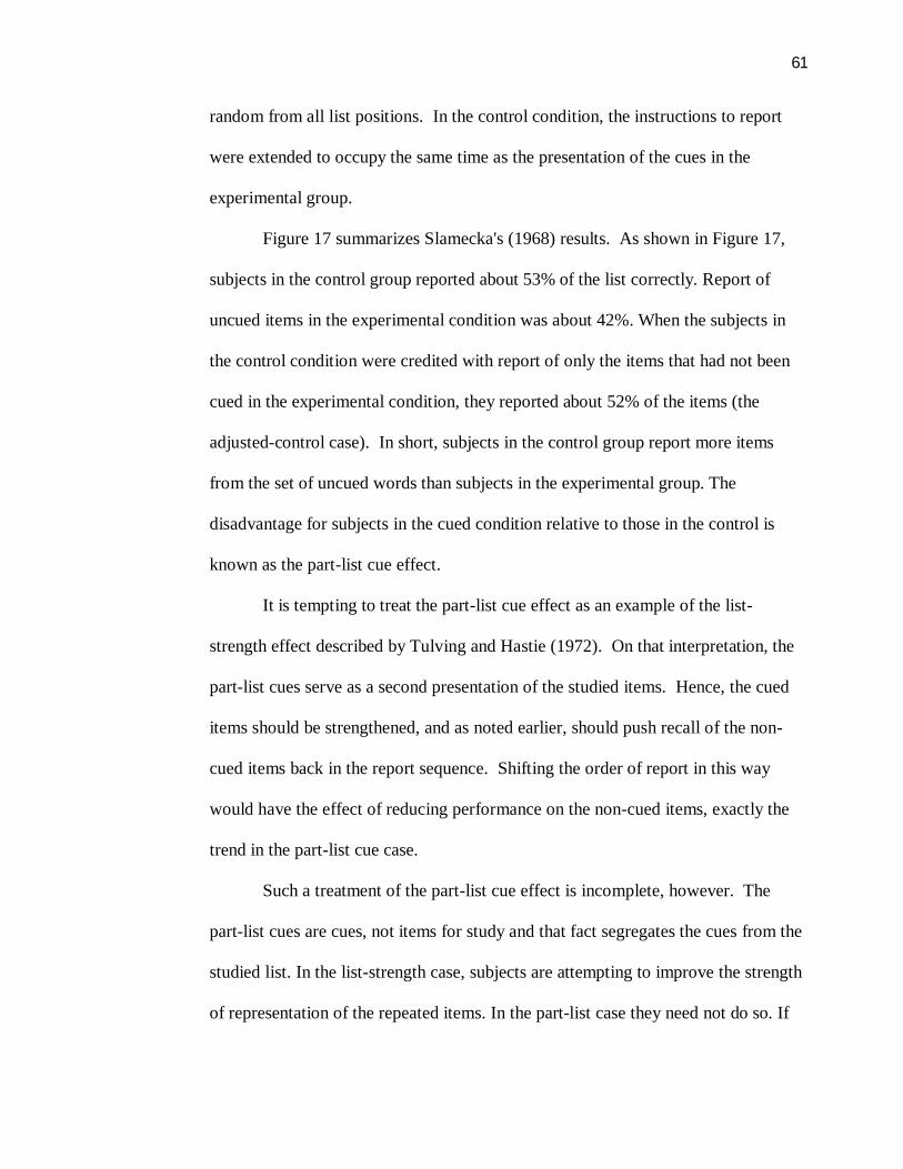
61
random from all list positions. In the control condition, the instructions to report
were extended to occupy the same time as the presentation of the cues in the
experimental group.
Figure 17 summarizes Slamecka's (1968) results. As shown in Figure 17,
subjects in the control group reported about 53% of the list correctly. Report of
uncued items in the experimental condition was about 42%. When the subjects in
the control condition were credited with report of only the items that had not been
cued in the experimental condition, they reported about 52% of the items (the
adjusted-control case). In short, subjects in the control group report more items
from the set of uncued words than subjects in the experimental group. The
disadvantage for subjects in the cued condition relative to those in the control is
known as the part-list cue effect.
It is tempting to treat the part-list cue effect as an example of the list-
strength effect described by Tulving and Hastie (1972). On that interpretation, the
part-list cues serve as a second presentation of the studied items. Hence, the cued
items should be strengthened, and as noted earlier, should push recall of the non-
cued items back in the report sequence. Shifting the order of report in this way
would have the effect of reducing performance on the non-cued items, exactly the
trend in the part-list cue case.
Such a treatment of the part-list cue effect is incomplete, however. The
part-list cues are cues, not items for study and that fact segregates the cues from the
studied list. In the list-strength case, subjects are attempting to improve the strength
of representation of the repeated items. In the part-list case they need not do so. If

62
subjects treat the cues as cues, not list items for study, the mechanism that yields the
list-strength effect does not apply.
To simulate the Slamecka (1968) experiment, the model was presented with
a list of 30 items repeated in two blocks using different random orders, as in
Slamecka's task. As before, the item weights increased geometrically across the two
blocks, and the associative weights decreased across the two blocks. Because the
words were repeated in different random orders on the two blocks, the final weights
applied to the 30 individual study items were no longer simple geometric functions
of list position.
The model was fit to the control condition and the fitted parameters used in
the cued condition. For the cued condition, half of the studied items were selected at
random, and encoded as a continuation of the two previous lists. ` In recall, instead
of starting report using the end-of-list item as a probe, a cue was picked from the set
of cue items at random. The cue was used to initiate recall. During recall, if the
model attempted to report a cue item, report was suppressed, and the lexicon was
not updated, but the cue item was used as the next probe. Non-cue items were
reported in the usual fashion and were used as the next probe. When recall halted,
the model picked an unused cue to re-start recall. The model continued until all the
cue items had served as probes.

63
Figure 17. Percent words recalled correctly as a function of the type of cue and scoring criterion.
The hatched columns show data from Slamecka (1968, Table 1, common words); the open columns
show the corresponding data from the simulation.
Figure 17 shows the results of the simulation along with the data from the
Slamecka (1968) study. As is clear in Figure 17, the model matched the empirical
data for the cued conditions remarkably well, even though there were no changes in
parameters across the conditions; the part-list inhibition comes for free.
In Slamecka's (1968) task, the cues were available to the subject throughout
the recall period. In subsequent work, the cues were presented and then removed.
When the cues are presented, they can be provided in the same order as they
appeared in the study list (congruent cuing) or in a scrambled order (incongruent
cuing). There is part-list cuing interference in both cases, but the interference is
Control Adjusted Cued0
10
20
30
40
50
60
70
Perc
ent R
ecal
l
Condition
Data Simulation

64
greater when the cues are scrambled relative to the order in which they were studied
(Sloman, Bower, & Rohrer, 1991). In addition, subjects are sometimes prohibited
from reporting the cued items and sometimes allowed to report the cued items.
According to Roediger, Stellon, and Tulving (1977), prohibiting report of the cued
items decreases interference.
To demonstrate that the model can handle the congruent-cue effect, I
simulated Experiment 1 from Sloman, Bower, and Rohrer (1991). In their
experiment, 24 items were presented for study and half of the studied items (items
from the odd list positions) were used as part-list cues, either in the same order as
they had been studied or in a scrambled order. In a control condition, the same
items were present for study and immediate free recall.
Figure 18 (top panel) summarizes the results from the Sloman, Bower, and
Rohrer (1991) experiment. As is clear in the figure, both kinds of part-list cue
reduced critical recall relative to the control, and the inhibition was greater for the
incongruent-cue condition than for the congruent-cue condition.

65
Figure 18. Percent correct recall of non-cued items as a function of the type of cue. The upper
panel shows data taken from Sloman, Bower and Rohrer (1991, Experiment 1). The bottom panel
shows data taken from the simulation. In the control condition, no cues were administered, and the
recall score is based on the items not cued in the other conditions.
To simulate the experiment, the model was first fit to the control condition
using a 24-item list studied once, and then the parameters so derived were used in
the two part-list cue conditions. In the congruent part-list condition, items from the
odd list positions were used as cues. In the incongruent condition, the same items
were used as cues, but in scrambled order. The cues were used in the predetermined
order appropriate to the condition, and the recall procedure was the same as in the
simulation of the Slamecka (1968) experiment.
Control Congruent Incongruent30
35
40
Data
Control Congruent Incongruent30
35
40Simulation
Perc
ent C
orre
ct R
ecal
l
Condition

66
Figure 18 (bottom panel) shows the results of the simulation. Report of the
non-cued items in the control case was considerably better than in any of the cued
cells. There was an advantage for the congruent-cue condition over the incongruent-
cue condition. The results match the data from Sloman, Bower, and Rohrer (1991)
remarkably well; both the part-list interference and the congruent/incongruent
effects came for free.
Part-list cuing inhibits report of the non-cued items because the explicit cue
upsets the normal order in which items are retrieved. Usual retrieval organization
gives preference to items at the ends of the list (where either item or associative
information is strongest). Retrieved items serve as cues for the next report; hence,
report spreads from the preferred items. In part-list cuing, by contrast, an arbitrary
item starts the report and
report cannot be organized in the usual fashion. Scrambling the order of the cues, as
in the incongruent condition, compounds the problem.
Categorized lists
When presented with lists containing words from several distinct conceptual
categories (e.g., the name of professions, mammals, makes of automobile, etc),
subjects tend to cluster their recall by category (e.g., Bousfield & Sedgewick,
1944). Bousfield (1953) showed that the structure of a categorized list benefits
recall even when the lists are presented in random order, although it is clearly
helpful to present the words category by category (i.e., subjects can exploit the
categorization more effectively when it has been made explicit).

67
Clustering suggests an active organizational process. The process,
presumably, would recognize and exploit the category relationships in order to
build units based on semantic relationships. In keeping with my overall theoretical
position, however, it seemed reasonable to inquire whether an active organizational
process is required. Perhaps, clustering reflects the associative structure within the
lexicon without requiring an extra mechanism to exploit the relations within
categorized lists.
Dallet (1964) provided clear examples of clustering using common high-
frequency words. In one experiment, he presented subjects with 12-word lists. In a
control condition, the words were selected randomly from his word pool. For the
categorized lists, the words were representatives of four common conceptual
categories. The categorized lists were presented to the subjects in two ways: For
one group of subjects, the categories were blocked; that is, the words from a
particular category were presented one after the other. For another group of
subjects, the categorized words were presented in scrambled order. Hence, the
experiment involved three groups, a control condition with unrelated words, and
two conditions with categorized lists, one blocked by category and one randomized
across categories.
Figure 19 summarizes Dallet’s (1964) results. As is shown in the top panel,
recall in the control condition was lower than in either of the categorized-list
conditions. In addition, recall was greater with blocked presentation than with
random presentation. The bottom panel shows a cluster score (Bousfield, 1953) that
represents the extent to which the subjects clustered members of the same category

68
together in their report (a higher score indicates greater clustering). When the
categorized lists were presented in random order, subjects were less able to cluster
the words than when the lists were blocked by category. Importantly, the amount
recalled was correlated to the amount of clustering.
Dallet’s (1964) control condition was a 12-item free-recall experiment that
the current model handles directly. The categorized list conditions, however, require
us to extend the representation of words to include categorized items.
Words within a category should be related to one another more highly than
words across categories. The precise nature of the relation is unclear. Current
accounts of similarity postulate feature overlap (Rogers & McClelland (2004)
and/or a higher level of intra-category association than inter-category association.
Operationally, an experimenter who wishes to use a categorized list first selects
words so that the similarity and associative links are high for the words within a
category relative to those across categories (see Postman & Keppel, 1970).
Categorization may well include other correlated properties of the words. I
modeled a categorized list by constructing vectors so that they were both similar (as
measured by the dot-product) and had a higher degree of association than unrelated
words in the lexicon.
Dallet (1964) used four categories of three items each. To simulate his
study, four sets of three vectors were created so that the three vectors within a set
were similar to each other (see Murdock, 1995, for the technique). The similarity
was set by a parameter . Secondly, associations among all pairs of items within
each category in the lexicon were strengthened, but we did not strengthen the

69
associations of pairs of items across categories. The additional strength was
controlled by a parameter .
To fit Dallet’s (1964) data, mean recall in the control condition was first fit
to obtain parameters. Then the model’s encoding parameters were frozen, and mean
recall in the blocked condition was fit to estimate values of and . Finally, all
parameters were frozen and a condition representing the random-order categorized
case was simulated. To obtain stable data, 20 runs of 500 simulated trials were run
in each condition.
Figure 19 shows the results of the simulation along with Dallet’s (1964)
data. As is clear in the top panel of the figure, the model matched mean recall for
the control data almost exactly. After freezing the model’s parameters, mean recall
in the blocked

70
Figure 19. The top panel presents mean number of items reported correctly as a function of material
and categorization condition. The hatched columns present data from Dallet (1964). The open
columns present the data from the model. The bottom panel shows the mean cluster score as a
function of categorization condition corresponding to the random and blocked conditions in the top
panel.
condition was fit to estimate categorization parameters, and again, the simulation
was able to match mean recall almost exactly. Finally, all parameters were frozen
and the items were presented in random order to obtain performance for the random
condition. As is clear in the figure, the model matched mean recall almost perfectly.
In other words, the model was able to fit a block-categorized list correctly by
adding parameters needed to describe the character of the list ( and ), and, armed
02468
1012
Mea
n C
orre
ct R
ecal
lBlocked Random Control
Data Simulation
0
1
2
3
4
5
Mea
n C
lust
er S
core
Blocked Random

71
with the latter parameters, the model anticipated the advantage for blocked over
random presentation without re-fitting.
The bottom panel of Figure 19 shows the cluster scores obtained by scoring
the responses produced by the model in the two categorized list conditions. The
cluster score was not used in fitting the data; hence, the close fit of the data by the
model is entirely a free prediction.
As is clear in Figure 19, the model correctly matched a representative
clustering experiment without recourse to an extra control mechanism. By building
categorized lists, variance in associations among words in a subject’s lexicon has
been acknowledged. Recalling Simon’s parable of the simple ant walking a
complex path, the complexity is in the lexicon, not in the processing mechanism.
That is, an active, on-line organizational process is unnecessary to account for
clustering over and above the similarity and associative relationships already
present in the lexicon itself.
As an aside, the same principles used to model clustering can account for
the Deese-Roediger-McDermott (DRM) paradigm. Deese (1959) used the
Minnesota norms for the Kent-Rosanov items to measure frequency of response to a
set of critical words. He then gave subjects word-lists composed of the 12 highest
frequency responses to a critical word. The critical word would regularly show up
as an extra-list intrusion. Roediger and McDermott (1995) replicated Deese (1959).
There has been work done in the literature on priming which casts some
doubts on frequency of response being a pure measure of association. Lucas (2000)
did a macro-analytic study of priming experiments and concluded that there was

72
evidence for pure semantic priming due to item overlap, and that there was no
evidence for pure associative priming. Hutchison (2003) criticized Lucas’ work
and performed a micro-analytical study of those experiments in the Lucas study he
felt could be compared statistically, and added a few more studies. His analysis was
thorough and his reasoning sound.
Hutchison (2003) looked upon the source of priming to be an indicator
distinguishing between holistic and distributed theories of priming. Holistic models
use spreading activation between associated nodes in a network to account for
priming. Distributed models consider priming to be a product of feature overlap
between representative items in semantic memory. “The most important conclusion
is that automatic priming appears to be due to both association strength and feature
overlap” (Hutchison, 2003). As shown in the previous account of clustering, this
model is capable of representing feature overlap and associative activation. The
DRM effect is no challenge for this model.
I should note here that I do not consider this model a spreading-activation
model. The term spreading activation is one that has been co-opted by neural net
modelers. These nets have no representation assumptions, and accordingly cannot
represent feature overlap. This particular model stands out among its peers, in that it
captures both associative information, and feature overlap. I have quoted those who
have used the word activation, but I have not once used the word activation when
describing this model. The word strength has been used instead.

73
Chapter 6: Mistaken Assumptions in Scoring Order of Report
Learning over trials has been ignored by those who have examined free
recall data. This disregard of learning results from an assumption that, because on
each trial different words are presented, there is no need for subjects to learn. I will
show that, although subjects do not need to learn list items over trials, they do learn
to perform the task differently across trials. In effect, there are strategic changes in
the way subjects order report across trials.
To one familiar with measures of order in free recall, it may seem that using
Kendall’s τ in preference to the Output Position Curve (OPC) (Nilsson, Wright,
Murdock, 1975) is a fault in our analysis. Michael Kahana (1996) states that, if list
presentation is auditory, subjects begin free recall about 3 items back from the end
of the list and work toward lists end, while in visually presented lists, the subjects
begin recall at the last list item and then work backward for the first few reports.
The argument, first put forward by Nilsson et al. (1975), is now widely accepted.
The idea that report order for auditory presentation differs substantially from
ordering in visual presentation is inspired by examining data averaged over all
experimental trials. The Conditional Probability of Response Curve (CRP), another
measure of order advanced by Kahana (1996), is also formed by averaging across
all experimental trials. I examined both of these order of report scores carefully.
Using data from Murdock (1962) 20 item lists presented at 1 word per
second, I examined groups of auditory presentation trials in an orderly progressive

74
manner. Figure 20 shows the OPC curve for groups of 10 trials in ascending order.
0 5 10 15 202
4
6
8
0 5 10 15 202
4
6
8
0 5 10 15 202
4
6
8
0 5 10 15 202
4
6
8
Mea
n O
utpu
t Pos
ition
Presentation Position
Trials 1 to 10
Mea
n O
utpu
t Pos
ition
Presentation Position
Trials 11 to 20
Mea
n O
utpu
t Pos
ition
Presentation Position
Trials 36 to 45
Mea
n O
utpu
t Pos
ition
Presentation Position
Trials 71 to 80
Figure 20. The OPC curves for groups of ten trials in ascending order. The data are drawn from
Murdock (1962) 20 items lists presented at 1 word per second.
An examination of the graphs reveals that trials one to ten show no hook
occurring at the end of the OPC curve. Subjects are tending to begin recall with the
last presented item and recall backward for a number of outputs before switching to
the first presented items.

75
-6 -4 -2 0 2 4 60.0
0.1
0.2
0.3
0.4
-6 -4 -2 0 2 4 60.0
0.1
0.2
0.3
0.4
-6 -4 -2 0 2 4 60.0
0.1
0.2
0.3
0.4
-6 -4 -2 0 2 4 60.0
0.1
0.2
0.3
0.4
Con
ditio
nal R
espo
nse
Pro
babi
lity Trials 1 to 10
Lag
Trials 36 to 45 Trials 71 to 80
Trials 11 to20
Figure 21. CRP curves for ascending groups of trials from the same data set used in Figure 19. The
tendency of forward ordering of report to increase as trials increase is apparent.
We would expect the CRP curve to show a stronger tendency to forward
report order as trials proceed, as the tendency to forward recall of the last few list
items grows.
Figure 21 shows the CRP curves for the same trial groupings used in Figure 20. An
examination of Figure 21 fulfills this expectation.
Figure 22 shows the mean number of words recalled per trial for each of the
ten- trial blocks shown in Figures 20 and 21. As can be seen in Figure 22, number
of words recalled per trial does not seem to change as recall order changes.

76
Trials 1 to 10 Trials 11 to 20 Trials 46 to 55 Trials 71 to 800
1
2
3
4
5
6
7
Mea
n W
ords
Rec
alle
d pe
rTria
l
Figure 22. Mean words recalled per trial for each of the four ten-trial blocks in Figures 19 and 20.
The tendency for the hook in the OPC curve to grow and for the CRP to
show increasing forward order as a function of trials presented is not just present in
the list length and presentation rate presented in Figures 20 and 21. Figures 23 and
24 show the OPC and CRP curves, respectively, for ascending groups of trials. The
data are taken from Murdock (1962) 10 item lists presented at a rate of 1 word
every 2 seconds. The tendency for the hook in the OPC curve to appear and then
grow as trials progress is clear. The growth over trials of forward report in the CRP
curve is also readily apparent. The tendency for progressive changes over trials in
both of these order-of-report scores is apparent in all list lengths and for both
presentation rates in the Murdock (1962) data sets.

77
0 2 4 6 8 102
3
4
5
6
0 2 4 6 8 102
3
4
5
6
0 2 4 6 8 102
3
4
5
6
0 2 4 6 8 102
3
4
5
6
Mea
n O
utpu
t Pos
ition
Trials 1 to 10 Trials 11 to 20
Trials 36 to 45
Presentation Position
Trials 71 to 80
Figure 23. The OPC curves for groups of ten trials in ascending order. The data is drawn from
Murdock (1962) 10 items lists presented at 1 word per 2 seconds.
-6 -4 -2 0 2 4 60.0
0.1
0.2
0.3
0.4
0.5
-6 -4 -2 0 2 4 60.0
0.1
0.2
0.3
0.4
0.5
-6 -4 -2 0 2 4 60.0
0.1
0.2
0.3
0.4
0.5
-6 -4 -2 0 2 4 60.0
0.1
0.2
0.3
0.4
0.5
Con
ditio
nal P
roba
bilit
y of
Rec
all
Trials 1 to 10 Trials 10 to 20
Trials 36 to 45
Lag
Trials 71 to 80
Figure 24. CRP curves for ascending groups of trials from the same data set used in Figure
21. The tendency of forward ordering of report to increase as trials increase is apparent.
In the Murdock (1962) free-recall experiments, auditory presentation was
used with all lists. There were eighty trials in each condition, and for each condition
it took at least 20 trials for the hook to begin to show, and more than 30 trials for it

78
to predominate. Visually presented lists examined by Nilsson, Wright and Murdock
(1975) used a total of 25 trials per experiment. Murdock and Olsson (1970)
visually presented lists using only 20 trials per experiment. In both of these cases, it
is unreasonable to expect any developing hook in the OPC curve to predominate if
the curve is formed by averaging across all trials in these experiments. I chose to
examine the Murdock and Okada data by comparing the OPC of the first four trials
with that of the last four trials. I examine their slow (1 word per sec.) and their fast
(2 words per sec.) visual presentation conditions. Figure 25 shows the OPC and
CRP curves for the slow condition. Figure 26 shows the same curves for the fast
condition.
-6 -4 -2 0 2 4 60.0
0.1
0.2
0.3
0.4
-6 -4 -2 0 2 4 60.0
0.1
0.2
0.3
0.4
0 5 10 15 202
3
4
5
6
7
0 5 10 15 202
3
4
5
6
7Con
ditio
nal R
espo
nse
Prob
abilit
y
Lag
Trials 1 to 4
Lag
Trials 16 to 20
Mea
n O
utpu
t Pos
ition
Presentation Position
Figure 25. OPC and CRP curves for groups of trials from Murdock & Okada (1970) slow condition.
The tendency of forward report to increase along with a hook to appear as trials increase is
apparent.

79
-6 -4 -2 0 2 4 60.00
0.05
0.10
0.15
0.20
0.25
0.30
0.35
-6 -4 -2 0 2 4 60.00
0.05
0.10
0.15
0.20
0.25
0.30
0.35
0 5 10 15 202.0
2.5
3.0
3.5
4.0
4.5
5.0
5.5
6.0
0 5 10 15 202.0
2.5
3.0
3.5
4.0
4.5
5.0
5.5
6.0C
ondi
tiona
l Res
pons
e P
roba
bilit
y
First Four Trials
Lag
Last Four Trials
Mea
n O
utpu
t Pos
ition
Lag
Presentation Position
Figure 26. OPC and CRP curves for groups of trials from Murdock & Okada (1970) fast condition.
The tendency of forward report to increase along with a hook to appear as trials increase is again
apparent.
Figures 24 and 25 make it apparent that the same progression from
backward to increasing forward recall occurs in free-recall with visual presentation
as well as auditory presentation.
It seems easy to speculate that somehow subjects anticipate the end of the
list and use their estimate and anchor it to the second, third or fourth last item to
begin recall. Roberts (1972) performed an experiment which would seem to rule out
this possibility. Roberts gave subjects lists of length ten, twenty, thirty or forty
words. Lists were grouped by presentation modality, and by presentation rate. List
length was randomized across trials, preventing anticipation of the end of the list.
Figure 27 illustrates the OPC curve of Roberts’ data for twenty item lists with
auditory and visual presentation at 1 or 2 words per second.

80
As can be seen, the OPC curves are hooked under all conditions, even though end
of list could not be anticipated.
0 5 10 15 202
4
6
8
10
0 5 10 15 202
4
6
8
10
0 5 10 15 202
4
6
8
10
0 5 10 15 202
4
6
8
10
Visual Presentation 2 words per Second
Mea
n O
utpu
t Pos
ition Visual Presentation
1 word per Second
Auditory Presentation 2 words per Second
Auditory Presentation 1 word per Second
Presentation Position
Figure 27. Mean Output Position Curves for Roberts (1972) 20 item lists with visual or auditory
presentation at one or two words per second.

81
Chapter 7: Limitations of the Model
Regarding the previous chapter’s contents, the present model does not
account for the shift in report strategy across trials. I take heart, however in that the
model does account for subject’s initial trials. Regardless of what subjects are
doing, whether an automatic process is occurring, or subjects are consciously
attempting to improve recall, I do not address the issue of changing recall strategy
in this paper. A goodly amount of empirical work needs to be done to tease out the
reason for the changes in report order across trials. It could be that subjects begin to
split supra-span lists into two lists and recall each in a forward order. It could also
be that subjects tend to stop trying to associate middle of list items and use the
associative capacity they save to associate end of list items more strongly. It could
be that neither of these explanations is correct and something as yet unforeseen is
occurring.
No one else has as yet developed a model of memory that explains this
phenomenon. Kahana (1996) added two new parameters to SAM and allowed the
size of the output buffer in SAM to vary randomly between 3 and 7 to obtain a fit
that came close to the actual hook in Murdock’s data. The shape of the OPC for the
first twenty trials would have been very similar to the last twenty trials in this fit.
Kahana (1996) is a fine example of a good fit which does not explain the
phenomenon. Given enough free parameters, we might fit anything, and SAM has
plenty of free parameters.
There is a further limitation possessed by the model. Unrealistically, it
treats each trial as an independent event because it generates a new vocabulary for

82
each trial. The model’s limited vocabulary has forced this constraint. In the real
world, each subject has a unique lexicon, and that subject’s lexicon is in place for
all trials. In defence of the present model, other models either retain the same
vocabulary for all subjects, or use independence of trials as I have. We now have tools to
rectify this situation.

83
Chapter 8: An Updated Model
Since the development of the model presented in the last section, The High
Performance Computing Virtual Laboratory (HPCVL) has undergone a large
number of upgrades. Each node has CPU’s of far faster chip speed. Memory has
been expanded tremendously. And the addition of libraries from the Numerical
Algorithms Group (NAG) allows for the parallel computation of circular
convolution. I have used these improved tools to upgrade the model. It allows me
to explore potential boundary conditions for the holographic representation that is at
the core of the model. The hologram involves superimposing item and associative
vectors. At some point, numeric resolution may limit the hologram’s utility. It is
necessary to show, therefore, that the potential exists for expansion to a vocabulary
size that maps more closely onto the human lexicon.
Items are represented by vectors f0, f1, f2, … fN, where N = 5000. Circular
convolution and circular correlation now replace linear convolution and correlation.
Less information is lost when circular convolution and correlation are used. I
explain these two processes in Appendices C and D respectively.
The lexicon has been expanded from 500 to 5000 item vectors, and the
concomitant 12,502,500 associations. The parameters Π and are used in the
updated model as direct scaling parameters on items and associations respectively.
Both Π and have been set to value 0.001 in the following simulation. A new
lexicon is created for each subject. The subject retains that lexicon throughout all
trials of the simulated experiment. Because trials are not independent within
subjects, the updated model requires one more parameter. After recalling as much

84
as they can, subjects may use the time left in the recall interval to notice things like
a shadow on the wall of the experimental lab. This activity would tend to cause
overwriting of vocabulary items. Each item, I, in the vocabulary has its strength Si
reduced according to the equation
Si = Si – Si ψ , where ψ is a fixed parameter of the model. Though a few things
have changed, the updated model retains all aspects of the theory represented by the
previous version.
5 10 15 200
20
40
60
80
100
5 10 15 200
20
40
60
80
100
Perc
ent C
orre
ct R
ecal
l
Presentation Position
Murdock (1962)20 words at 1 word/s
Figure 28. The solid line represents the serial position curve for Murdock (1962) twenty item lists
presented at 1 word per second. The vertical bars show the range of outputs from twenty runs of
the updated model.
I used the updated version to fit and then simulated the first ten trials of the
Murdock (1962) twenty item lists at 1 word per second. When fitting the updated
model, I fit to both the Serial Position Curve of the data, and to the values at

85
positions -1 and +1 of the CRP curve. This was done to constrain the OPC curve,
and achieve a proper indication of the model’s behavior. Figure 28 shows the serial
position curve of Murdock’s data, and the range of scores from twenty runs of the
model.
The updated model captures the serial position curve as well as its
predecessor. Only the parameters have changed, which is to be expected using
circular correlation, and with a vocabulary ten times as large. The free parameters
used are shown in Appendix E.
Figure 29 shows the cumulative distribution of words correct per trial from
Murdock’s (1962) data, and the range of cumulative scores from the same 20
simulations
2 4 6 8 10 12 14
0.0
0.2
0.4
0.6
0.8
1.0
2 4 6 8 10 12 14
0.0
0.2
0.4
0.6
0.8
1.0
Cum
ulat
ive
Pro
porti
on
Words Correct per Trial
Cum
ulat
ive
Pro
porti
on
Words Correct per Trial
Figure 29. The cumulative distribution of words correct per trial from Murdock’s data, and the
range of cumulative scores from the same 20 simulations of the updated model that gave us the
serial position curve of Figure 27.

86
of the model that gave us the serial position curve of Figure 28. Again, we have an
excellent coverage of the data by the model.
-5-4 -3-2 -1 0 1 2 3 4 50.00
0.02
0.04
0.06
0.08
0.10
0.12
0.14
0.16
0.18
-5 -4 -3-2-1 0 1 2 3 4 5
Con
ditio
nal R
espo
nse
Pro
babi
lity
Lag
Figure 30. CRP curves from the first ten trials of Murdock (1962) 20 item lists presented at I word
per second. The left hand curve is drawn from the data. The right hand curve represents the
simulation from the updated model.

87
5 10 15 20
2
3
4
5
6
7
8
5 10 15 20
2
3
4
5
6
7
8
Mea
n O
utpu
t Pos
ition
Presentation Position
Figure 31.The OPC curve of the first ten trials of the Murdock (1962) twenty item list at 1 word per
second. The solid line is the data. The vertical lines represent the range of values derived from 20
runs of the updated model.
Figures 30 and 31 show the CRP and OPC curves respectively of the data
and the simulation. Figure 31 shows that the model gives an excellent prediction of
the OPC curve. In effect, recall ordering in the model matches that of experimental
subjects.
The updated model no longer uses the assumption of independent trials but
retains it the capabilities of the previous model. It is a more complete account. The
free parameters used in this fit are shown in Appendix G.
The increased vocabulary size (by an order of magnitude) did not strain the
resolution of the hologram. A vocabulary of 5000 is still an order of magnitude

88
smaller than human vocabulary, but testing the resolution further faces
technological limits. The issue remains open, but my expectation is that a
holographic control remains a viable option.

89
Chapter 9: Discussion
The evidence presented here is that accuracy and order of report in free
recall can be understood in terms of changes in the momentary strength of the
words during recall. To make the point, I applied a strength-based model to the
basic free-recall task and to several variations on it. The model postulates (a) that
studying a list changes the resting strength of items and associations in the lexicon,
(b) that selection for report is based on a combination of item and associative
information, and (c) that reporting an item produces feedback that changes the
resting strength of items in the lexicon.
When applied the to free-recall experiments, the model captures several
important details of performance, including the serial-position curve, intrusions
from extra-list vocabulary items, order of report, and trial-to-trial variability on
accuracy of recall.
I subsequently applied the model to extensions of the immediate free-recall
task. The extensions included list-strength, part-list cuing, distraction, and
clustering experiments. In all cases, the model captured the pattern of performance
and provided fresh insight into how the paradigms relate to the basic free-recall
task. Importantly, the model successfully predicted features of performance without
re-fitting to obtain the performance in question.
A class of serial-recall models, known collectively as chaining models,
assume that subjects strengthen each item and associate it to its predecessor (e.g.,
Lewandowsky & Murdock, 1989). Unlike the earlier models, recall is based on a

90
combination of item and associative information and selection for report initiates
feedback to the lexicon.
The success of the model speaks to a number of theoretical issues. Consider
the argument for a short-term memory separate from the lexicon and the idea that
data are passed from one store to another. The idea of a limited- capacity short-
term memory system largely derives from limitations to performance and has roots
deep in the information-processing tradition in psychology (e.g., Miller, 1956).
Classic evidence for a separate short-term memory system is based on the
distraction paradigm (e.g., Craik, 1970; Glanzer & Cunitz, 1966). The present
model accounts for the critical data without invoking the idea of a separate short-
term memory store, although it does allow for fast fading strength of item
information due to overwriting. Hence, my evidence is that a separate store is not
necessary to explain the data. Performance in many short-term memory tasks may
be consistent with the idea of a separate store but evidence consistent with an
account does not force the conclusion.
Eric Kandel (2006) presents us with the fact that a change in synapse
strength can occur in two very different ways. One is a strengthening of the synapse
caused by the release of a greater quantity of neurotransmitter. This change is
relatively short lived, unless stimulation of the neural pathway is repeated, and
accounts for fast fading short-term storage. After several repeated bouts of
stimulation, the synapse is strengthened by the growth of new connections, which
can endure for hours, days, or indefinitely. However, unlike the account of short-
and long-term memory in the modal model, the change involves no movement from

91
one storage area to another. Kandel’s findings map directly onto my model in the
sense that an item’s strength may last for only a short time but that the item itself
resides in a long-term memory.
Although Kandel’s evidence points to a mechanism of short-term storage, it
is by no means clear how it maps onto the memory literature’s concept of short-
term storage. In particular, it is unclear the extent to which the mechanism can
explain the wealth of behavioural data associated with tests of the modal model’s
conception of short-term memory. My thesis is a demonstration that ideas about
short-term activation operating within a permanent storage system are competent to
account for the facts of free recall. To the extent that my ideas about short-term
activation operating within a permanent storage system map onto Kandel’s
mechanisms, my model’s success is a behavioural validation of his interpretation of
the physiological evidence.
Of the current conceptions of short-term memory in the human memory
literature, the model is closest to Cowan's (1988) idea that short-term memory can
be described in terms of items in the lexicon that are highly activated. In my
estimation, short-term activation in the long-term store has been mistakenly
attributed to a separate short-term store. I believe that the model's ability to account
for data thought to support the separate-memory-store idea shifts the burden of
proof to advocates of that position. Empirical evidence to force a conclusion is
urgently needed, especially in light of other evidence that argues for a strong long-
term memory component to tasks heretofore thought to tap short-term memory
(Hulme, Maughan, & Brown, 1991).

92
Next, the work acknowledges the fact that we know the words used in
memory experiments and the properties of our knowledge drive performance. The
idea is that control of report lies in the interaction of local events (studying and
reporting) with that knowledge. The approach could not work unless it is built to a
reasonable scale.
Chaining theories postulate that subjects encode overlapping pairs of items.
I suspect that encoding includes triples as well, but, as the model has demonstrated,
encoding of overlapping pairs provides a satisfactory approximation. What
distinguishes the model from earlier chaining theory is the way the encoded
information is used during retrieval. Both advocates and critics of chaining models
have assumed that retrieval ignores item information in favour of the associative
chain (see Lewandowsky & Murdock, 1989; Henson, Norris, Page & Baddeley,
1996). The theory represented in this thesis assumes that retrieval combines item
and associative information. The current evidence against chaining models is, in
fact, evidence against the idea of retrieval based only on the chain of associations.
I see no reason to postulate that subjects adopt conscious retrieval strategies
to accommodate the various applications of the basic free-recall task. As Sloman et
al. (1991) put the issue in connection with inhibition associated with part-list cuing,
“ascribing inhibition completely to disruption of conscious strategies as opposed to
more automatic retrieval processes seems unwarranted” (p. 975). I extend the same
principle to the list-strength effect, response clustering, and distraction paradigms:
encoding and retrieval based on item and associative strength guide retrieval
without the need of conscious strategies. Nevertheless, when considering data from

93
Murdock (1962), I selected data from the first trials because it appeared that
subjects changed strategy in later trials. The change may reflect a conscious
strategy shift; it may also reflect a less deliberate artifact of learning in the situation.
In its current form, the model does not consider learning; hence, I am, at this point
in time, reluctant to take a final position on the issue.
The model is based upon a linear system. Non-linear systems, such as
artificial neural networks, are both popular and more complicated than the simple
linear system that I have used. The current model's success argues strongly in
favour of a simple system, and shifts the burden of proof to proponents of non-
linear systems to show why the more complex system is necessary. Likewise,
retrieval is based on simple strength calculations; its success argues strongly in
favour of a simple strength-based system and shifts the burden of proof to
proponents of systems that implement rules or that require extra-list context
information to show why additional control processes are required.
The work was made possible by the availability of computational resources
large enough to allow implementation of the model and to fit it to data. The point is
not that the model is large but rather that the principles that allow it to work do not
apply with a small lexicon. The use of a 500-item vocabulary allows the model to
have sufficient variability among the items and among their associations.
Expanding the vocabulary allowed for the capture of data without the false premise
of independence across trials. In terms of Simon’s (1998) allegory of the ant
traversing a beach, by using a large vocabulary, the model has implemented a small
part of the complexity of the beach. Arguably, variance in lexical items is among

94
the least interesting aspect of those items—surely the semantics of lexical items is
more important for the subject—but the work is part of a growing body of evidence
that shows interesting properties of behaviour emerge when memory is modeled at
a large enough scale. Kwantes and Mewhort (1999) have shown, for example, that
many aspects of lexical access—including effects associated with word frequency,
spelling regularity, and syllable structure—occur without the need to invoke rules
or learned connections, but only if the lexicon is modeled at a sufficiently large
scale. Landauer and Dumais (1997) have shown that a good amount of semantic
information can be taken from usage of words if enough different contexts are
sampled (see also Lund & Burgess, 1996; Burgess, 1998; Jones & Mewhort, 2007).
The important lesson to take from such work is that the complexity of behaviour
can be traced to properties of the knowledge on which it is based. As a corollary,
an analysis of processing should start by considering knowledge at a sufficiently
large scale.
Tools from existing theory (TODAM) have been used to model the strength
of items and their associations in memory. Note, however, that this account is not
complete. We have demonstrated that strength considerations are sufficient to
predict report in free-recall paradigms. The strength calculations represent
constraints for a future process model, one that can fill in the details concerning
how items are retrieved.
A final and speculative extension of the work is to treat free-recall as a
laboratory model for thought itself. Subjective experience indicates that one
thought follows from another, but the nature of the control mechanism that

95
determines the flow of ideas remains an open question. John Locke speculated that
the flow of ideas reflects the pattern of associations among ideas. In his words,
Ideas that in themselves are not all of kin, come to be
so united in some men's minds, that it is very hard to
separate them; they always keep in company, and the
one no sooner at any time comes into the
understanding, but its associate appears with it
(Locke, 1690/1947, p. 198).
Locke's description sounds remarkably like a strength account of the flow of ideas
extended by the kind of combination of information mechanism illustrated in Figure
3. Perhaps our theory is a prototype for the kind of mechanism that Locke must
have had in mind when he argued “the whole gang, always inseparable, show
themselves together”.

96
References
Anderson, J. A. (1995). An introduction to neural networks. Cambridge MA: MIT.
Anderson J. R., Bothell D., Lebiere C., & Matessa M. (1998). An integrated theory of list
memory. Journal of Memory and Language, 38, 341–380
Atkinson, R. C., & Shiffrin, R. M. (1968). Human memory: A proposed system and its
control processes. In K. W. Spence & J. T. Spence (Eds.), The psychology of
learning and motivation Vol. 2 (pp. 89-195). New York: Academic Press.
Baddeley, A. D., & Hitch, G.J. (1977). Recency re-examined. In S. Dornic (Ed.), Attention
and Performance VI (pp. 647-667), Hillsdale, NJ: Erlbaum.
Bjork, R. A., & Whitten, W., B. (1974). Recency-sensitive retrieval processes in long-term
free recall. Cognitive Psychology, 6, 173-189.
Boudewijnse, G.-J., Murray, D. J., & Bandomir, C. A. (1999). Hebart’s mathematical
psychology. History of Psychology, 2, 163-193.
Bousfield, W. A. (1953). The occurrence of clustering in the recall of randomly arranged
associates. Journal of General Psychology, 49, 229-240.
Bousfield, W. A., & Sedgewick, C. H. W. (1944). An analysis of sequences of restricted
associative responses. Journal of General Psychology, 63, 233-238.
Bracewell, R. N. (1986). The Fourier transform and its applications (2nd Ed.). New York:
McGraw Hill.
Brown, G.D.A., Preece, T., & Hulme, C. (2000). Oscillator-Based memory for serial order,
Psychological Review, 107, 127-181.

97
Burgess, C. (1998). From simple associations to the building blocks of language: Modeling
meaning in memory with the HAL model. Behavior Research Methods, Instruments
& Computers, 30, 188-198.
Cowan, N. (1988). Evolving conceptions of memory storage, selective attention, and their
mutual constraints within the human information processing system. Psychological
Bulletin, 104, 163-191.
Cowan N. 1993. Activation, attention, and short-term memory. Memory and Cognition, 21,
162-167.
Craik, F. I. (1970). Fate of primary memory items in free recall. Journal of Verbal
Learning and Verbal Behavior, 9, 143-148.
Craik, F. I., & Lockhart R. S. (1972). Levels of processing: A framework for memory
storage. Journal of Verbal Learning and Verbal Behavior, 11, 671-684.
Craik, F. I., & Watkins, M. J. (1973). The role of rehearsal in short-term memory. Journal
of Verbal Learning and Verbal Behavior, 12, 599-607.
Dallet, K. M. (1964). Number of categories and category information in free recall. Journal
of Experimental Psychology, 68, 1-12.
Davelaar, E. J., Goshen-Gottstein, Y., Ashkenazi, A., Haarmann, H. J., Usher, M. (2005).
The demise of short-term memory revisited: Empirical and computational
investigations of recency effects. Psychological Review, 112, 3-42.
Deese, J. (1959). On the prediction of occurrence of particular verbal intrusions in
immediate recall. Journal of Experimental Psychology, 58, 17-22.

98
Ebbinghaus, H. E. (1885). Das Gedächtnis: Untersuchungen zur experimentellen
Psychologie. Leipzig: Duncker and Humboldt. Reprinted as Ebbinghaus H. E.
(1964). Memory: A contribution to experimental psychology. New York: Dover.
Estes, W. K. (1972). An associative basis for coding and organization in memory. In A. W.
Melton & E. Martin (Eds.), Coding Processes in Human Memory, Washington:
V.H. Winston & Son.
Estes, W. K. (1997). Processes of memory loss, recovery, and distortion. Psychological
Review, 104, 148-169.
Franklin, D. R. J., & Mewhort, D. J. K. (2002). An analysis of immediate memory: The
free-recall task. In N. J. Dimpoloulos & K. F. Li (Eds.), High Performance
Computing Systems and Applications 2000 (pp. 465-479). New York: Kluwer.
Glanzer, M., & Cunitz, A. R. (1966). Two storage mechanisms in free recall. Journal of
Verbal Learning and Verbal Behavior, 5, 351-360.
Godden, D.R., & Baddeley, A.D. (1975). Context-Dependent memory in two natural
environments: On land and underwater. British Journal of Psychology, 66, 325-331.
Gold, P. E., & King, R. A. (1974). Retrograde amnesia: Storage failure versus retrieval
failure. Psychological Review, 81, 465-469.
Hebb, D. O. (1949). Organization of behavior. New York: Wiley.
Hebb, D. O. (1961). Distinctive features of learning in the higher animal. In J. F.
Delafresnaye (Ed.), Brain mechanisms and learning (pp. 37-46). Oxford:
Blackwell.

99
Henson, R. N. A., Norris, D. G., Page, M. P. A., & Baddeley, A. D. (1996). Unchained
memory: Error patterns rule out chaining models of immediate serial recall.
Quarterly Journal of Experimental Psychology, 49A, 80-115.
Hockley, W. E. (1992). Item versus associative information: Further comparisons of
forgetting rates. Journal of Experimental Psychology: Learning Memory and
Cognition, 18, 1321-1330.
Howard, M. W., & Kahana, M. J. (2002). A distributed representation of temporal context.
Journal of Mathematical Psychology, 46, 269-299.
Hubel, D H., & Wiesel, T. N. (1979). Brain mechanisms of vision. Scientific American,
241, 150-162.
Hulme, C., Maughan, S., & Brown, G. D. A. (1991). Memory for familiar and unfamiliar
words: Evidence for a long-term memory contribution to short-term memory span.
Journal of Memory and Language, 30, 685-701.
Hutchison, K. A. (2003). Is semantic priming due to association strength or feature
overlap? A microanalytic review. Psychonomic Bulletin & Review, 10, 785-813
Jones, M. N., & Mewhort, D. J. K. (2007). Representing word meaning and order
information in a composite holographic lexicon. Psychological Review, 114, 1-37.
Kahana, M. J. (1996). Associative retrieval processes in free recall. Memory & Cognition,
24, 103-109.
Kahana, M. J., Sederberg, P. B., Howard, M.W. (2008). Putting short-term memory into
context: Reply to Usher, Davelaar, Haarmann, and Goshen-Gottstein (2008).
Psychological Review, 115, 1119-1126.

100
Kandel, E. R. (2006). In search of memory: The emergence of a new science of mind. New
York: W.W. Norton & Company.
Koppenaal, L., & Glanzer, M. (1990). An examination of the continuous distractor task and
the long-term recency effect. Memory & Cognition, 18, 183-195.
Kwantes, P. J., & Mewhort, D. J. K. (1999). Modeling lexical decision and word naming
as a retrieval process. Canadian Journal of Experimental Psychology, 53, 306-315.
Landauer, T. K., & Dumais, S. T. (1997). A solution to Plato's problem: The latent
semantic analysis theory of acquisition, induction, and representation of knowledge.
Psychological Review, 104, 211-240.
Lee, C. L., & Estes, W. K. (1981). Item and order information in short-term memory:
Evidence for multilevel perturbation processes. Journal of Experimental
Psychology: Human Learning & Memory, 7, 149-169.
Lewandowsky, S., & Murdock, B. B. (1989). Memory for serial order. Psychological
Review, 96, 25-57.
Locke, J. (1690 / 1947). An essay concerning human understanding. London: Dent.
Loeb, J. (1902). Comparative physiology of the brain and comparative psychology, New
York: G. P. Putnam's Sons.
Lucas, M. (2000). Semantic priming without association: A meta-analytic review.
Psychonomic Bulletin & Review, 7, 618-630.
Lund, K., & Burgess, C. (1996). Producing high-dimensional semantic spaces from lexical
co-occurrence. Behavior Research Methods, Instruments & Computers, 28, 203-
208.

101
Manning, S. K., & Pacifici C. (1983). The effects of a suffix-prefix on forward and
backward serial recall. The American Journal of Psychology, 96, 127-134
McGeogh, J. A. (1942). The psychology of human learning: An introduction. New York:
Longmans, Green and Co.
Mewhort, D. J. K., & Popham, D. (1991). Serial recall of tachistoscopic letter strings. In W.
E. Hockley & S. Lewandowsky (Eds.), Relating theory and data: Essays on human
memory in honor of Bennet B. Murdock (pp. 425-443). Hillsdale, NJ: Erlbaum.
Mewhort, D. J. K., Popham, D., & James, G. (1994). On serial recall: A critique of
chaining in the Theory of Distributed Associative Memory. Psychological Review,
101, 534-538.
Mewhort, D. J. K., Franklin, D. R. J., Sklair, N. (2008). How one idea leads to another.
Paper read at the annual meeting of the Canadian Society for Brain, Behaviour &
Cognitive Science, University of Western Ontario, June 19-21.
Miller, R. R. & Springer A. D. (1973). Amnesia, consolidation, and retrieval.
Psychological Review, 80, 69-79.
Murdock, B. B. (1962). The serial position effect of free recall. Journal of Experimental
Psychology, 64, 482-488.
Murdock, B. B. (1974). Human Memory: Theory and Data. Potomac, Md., Erlbaum.
Murdock, B. B. (1982). A theory for the storage and retrieval of item and associative
information. Psychological Review, 89, 609-626.
Murdock, B. B. (1995). Similarity in a distributed memory model. Journal of Mathematical
Psychology, 39, 251-264.

102
Murdock, B. B., & Okada, R. (1970). Inter-response times in single-trial free recall.
Journal of Experimental Psychology, 86, 263-267.
Nairne, J. S., & Neath, I. (1994). Critique of the retrieval/deblurring assumptions of the
Theory of Distributed Associative Memory. Psychological Review, 101, 528-533.
Nairne, J. S., Neath, I., Serra, M., & Byun, E. (1997). Positional distinctiveness and the
ratio rule in free recall. Journal of Memory and Language, 37, 155-166.
Neath, I. (1998). Human memory An introduction to research, data, and theory. Pacific
Grove, CA: Brooks/Cole.
Nelder, J. A., & Mead, R. (1965). A simplex method for function minimization. Computer
Journal, 7, 308-313.
Nilsson, L-G., Wright, E., & Murdock, B. B. (1975). The effects of visual presentation
method on single-trial free recall. Memory & Cognition, 3, 427-433.
Norman, D. A. (1970). Models of human memory. New York: Academic Press.
Page, M. P. A., & Norris, D. (1998). The Primacy Model: a new model of serial recall.
Psychological Review, 105, 761-781.
Plate, T. A. (1995). Holographic reduced representations. IEEE Transactions on Neural
networks. 6, 623-641.
Postman, L., & Keppel, G. (1970). Norms of word associations. New York: Academic
Press.
Press, W. H., Teukolsky, S. A., Vetterling, W. T., & Flannery, B. P. (1992). Numerical
recipes in FORTRAN The art of scientific computing (2nd Ed.). New York:
Cambridge University Press.

103
Raaijmakers, J. G. W. & Shiffrin, R.M. (1980). SAM: A theory of probabilistic search of
associative memory. In G. H. Bower (Ed.). The psychology of learning and
motivation: Advances in research and theory. (Vol. 14), (pp. 207-262). New York:
Academic Press.
Raaijmakers, J. G. W., & Shiffrin, R. M. (1981). Search of associative memory.
Psychological Review, 88, 93-134.
Ratcliff, R., Clark, S. E., & Shiffrin, R. M. (1990). List-strength effect: I. Data and
discussion. Journal of Experimental Psychology: Learning Memory & Cognition.
16, 163-178.
Roberts, S., & Pashler, H. (2000). How persuasive is a good fit? A comment on theory
testing. Psychological Review, 107, 358-367.
Roediger, H. L., & McDermott, K. B. (1995). Creating false memories: Remembering
words not presented in lists. Journal of Experimental Psychology: Learning,
Memory, and Cognition, 21, 803-814.
Roediger, H. L., Stellon, C. C., & Tulving, E. (1977). Inhibition from part-list cues and rate
of recall. Journal of Experimental Psychology: Human Learning and Memory, 3,
174-188.
Rogers, T. T. & McClelland, J. L. (2004). Semantic Cognition: A Parallel Distributed
Processing Approach. MA: MIT Press.
Ruchkin, D. S., Grafman, J., Camero K., & Berndt R. S. (2003). Working memory
retention systems: A state of activated long-term memory. Behavioral and Brain
Sciences, 26, 709–777.

104
Rundus, D., & Atkinson, R. C. (1970). Rehearsal processes in free recall: A procedure for
direct observation. Journal of Verbal Learning and Verbal Behavior, 9, 99-105.
Shiffrin, R. M. (1999). 30 years of memory. In C. Izawa (Ed.). On human memory:
Evolution, progress, and reflections on the 30th anniversary of the Atkinson-Shiffrin
model (pp. 17-33). Mahwah, NJ: Erlbaum.
Simon, H. A. (1996). The sciences of the artificial (3rd Ed.). Cambridge MA: MIT.
Slamecka, N. J. (1968). A case for response-produced cues in serial learning. Journal of
Experimental Psychology: Human Learning and Memory, 3, 222-232.
Sloman, S. A., Bower, G. H., & Rohrer, D. (1991). Congruency effects in part list cuing
inhibition. Journal of Experimental Psychology: Learning, Memory, and
Cognition, 17, 974-982.
Squire, L. R., & Wixted, J. T. (2011). The cognitive neuroscience of human memory since
H. M. The Annual Review of Neuroscience, 34, 259-288.
Tzeng, O. J. L. (1993).Positive recency effect in a delayed free recall. Journal of Verbal
Learning and Verbal Behavior, 12, 436-439.
Tulving, E. (1983). Elements of Episodic Memory. Oxford: Oxford University Press.
Tulving, E. (1974). Recall and recognition of semantically encoded words. Journal of
Experimental Psychology, 102, 778-787.
Tulving, E., & Hastie, R. (1972). Inhibition effects of intralist repetition in free recall.
Journal of Experimental Psychology, 92, 297-304.
Tulving, E., & Pearlstone, Z. (1966). Availability versus accessibility of information in
memory for words. Journal of Verbal Learning and Verbal Behavior, 5, 381-391.

105
Usher, M., Davelaar, E. J., Haarmann, H. J., Goshen-Gottstein, Y. (2008). Short-term
memory after all: Comment on Sederberg, Howard, and Kahana (2008).
Psychological Review, 115, 1108-1118.
Waugh, N. C., & Norman, D. A. (1965). Primary Memory. Psychological Review, 72, 89-
104.
Waugh, N. C., & Norman, D. A. (1968). Stimulus and response interference in recognition-
memory experiments. Journal of Experimental Psychology, 78, 551-559.
Weber, E. U. (1988). Expectation and variance of item resemblance distributions in a
convolution-correlation model of distributed memory. Journal of mathematical
Psychology, 32, 1-43.
Whitten, W. E., & Bjork, R. A. (1977). Learning from tests: Effects of spacing. Journal of
Verbal Learning and Verbal Behavior, 16, 465-478
Wickelgren, W. A. (1970). Multitrace strength theory. In D. A. Norman (Ed.), Models of
human memory (pp. 65-102). New York: Academic Press.
Wickelgren, W. A., & Norman, D. (1966). Strength models and serial position in short term
recognition memory. Journal of Mathematical Psychology, 3, 316-347.
Young, R. K. (1961). The stimulus in verbal learning. American Journal of Psychology, 74,
517-528.
Young, R. K. (1968). Serial learning. In T. R. Dixon & D. L. Horton (Eds.), Verbal
behavior and general behavior theory (pp. 122-148). Engelwood Cliffs, NJ:
Prentice Hall.

106
Appendix A
Linear Convolution Explained
Suppose two three component vectors, x and y.
x = x0, x1, x2 y = y0, y1, y2
The matrix of the cross product of x and y is:
The linear convolution of x and y will be called z. Vector z is formed by summing
components of the cross product vector that lay along the lines illustrated below.
x0y0 x0y1 x0y2
x1y0 x1y1 x1y2
x2y0 x2y1 x2y2
x0y0 x0y1 x0y2
x1y0 x1y1 x1y2
x2y0 x2y1 x2y2 z0
z1
z2
z-2
z-1

107
Appendix B
Linear Correlation Explained
Linear correlation is indicated by the # operator. Correlation is an
approximate inverse of convolution. If z = x*y, then correlating vector x with z (the
convolution of x and y) will yield a vector y’. Using the dot product of y and y’ as a
measure of similarity y and y’ are very similar, but not identical. The linear
correlation procedure is pictured below. Again, summation is done along the lines
shown.
z0x0 z0x1 z0x2 y' -2 z1x0 z1x1 z1x2 y' -1 z2x0 z2x1 z2x2 y' 0
y'1
y'2

108
Appendix C
Circular Convolution Explained
Suppose two three component vectors x and y.
x = x0,x1, x2 y = y0,y1, y2
The association, z, between x and y is represented as a vector formed by a circular
convolution (indicated by the * operator) of the associated item vectors. To better
understand this operation, I have illustrated it below.
First, the outer-product of x and y is formed.
The circular convolution of x and y will be called z. Vector z is formed by
summing components of the outer-product matrix that lay along the lines illustrated below.
x0y0 x0y1 x0y2
x1y0 x1y1 x1y2
x2y0 x2y1 x2y2
x0y0 x0y1 x0y2
x1y0 x1y1 x1y2
x2y0 x2y1 x2y2
z0
z1
z2

109
Appendix D
Circular Correlation Explained
Circular correlation is indicated by the # operator. Correlation is an approximate inverse of
convolution. Correlating vector x with z (the convolution of x and y) will yield a vector y’.
Using the dot product of y and y’ as a measure of similarity y and y’ are very similar, but
not identical. We first create the cross product of z and x.
The circular correlation procedure is pictured below. Again, summation is done along the
lines shown.
z0x0 z0x1 z0x2
z1x0 z1x1 z1x2
z2x0 z2x1 z2x2
z0x0 z0x1 z0x2 y'0 z1x0 z1x1 z1x2 y'1 z2x0 z2x1 z2x2 y'2

110
Appendix E
Fixed Parameters Used in the Simulations
Criterion 1.00
Bounds 1.00 0.70
Total Lexical Entries 500
N 521
0.15
15.95
0.029
0.00095

111
Appendix F
Free Parameters Used in the Simulations
Figure 0 0 tg tw
Representative Trial
3. 0 .230 0.307 0.839 0.836 -- -- -- --
Murdock & Okada (1970)
4. – 7. 0.209 0 .231 0.904 0.839 -- -- -- --
Murdock (1962
8. 1wd/s. 0.270 0.204 0 .905 0 .804 -- -- -- --
9. 1 wd/2 s. 0.245 0.292 0.896 0.821 -- -- -- --
Glanzer & Cunitz (1966)
12. 0.084 0.290 0 .962 0.850 1.16 0.407 -- --
Koppenaal & Glanzer (1990)
13. Control 0.230 0.307 0.839 0.836 -- -- -- --
Distraction 0.101 0.354 0.902 0.907 -- -- -- --
Tulving & Hastie (1972)
15. 0.270 0.204 0.905 0.829 -- -- 0.115 0.215
Slamecka (1968)
16. 0.334 0.295 0 .963 0.879 -- -- -- --
Sloman, Bower & Rohrer (1991)
17. 0.185 0.314 0.956 0.808 -- -- -- --
Dallet (1964)
18. Control 0.296 0.216 0.875 0.800 -- -- -- --
Blocked 0.296 0.216 0.875 0.800 -- -- 0.135 0.335
Random 0.296 0.216 0.875 0.800 -- -- 0.135 0.335

112
Appendix G
Parameters Used in the Updated Model
Fixed Parameters
Criterion 1.00
Bounds 1.00 0.70
Total Lexical Entries 5001
N 5001
15.95
0.001
0.001
Free Parameters
0 0.855023490
0 0.6601101
0.158516582
0.364528832
Ψ 5.84