A strain smoothing method in finite elements for structural...
220
A strain smoothing method in finite elements for structural analysis by Hung NGUYEN XUAN Docteur en Sciences appliqu´ ees de l’Universit´ e de Li` ege DES en M´ ecanique des Constructions, l’Universit´ e de Li` ege Bachelier en Math´ ematique et Informatique, l’Universit´ e des Sciences Naturelles de Ho Chi Minh Ville May 05 2008
Transcript of A strain smoothing method in finite elements for structural...

A strain smoothing method in finiteelements for structural analysis
by
Hung NGUYEN XUAN
Docteur en Sciences appliquees de l’Universite de LiegeDES en Mecanique des Constructions, l’Universite de Liege
Bachelier en Mathematique et Informatique, l’Universite des SciencesNaturelles de Ho Chi Minh Ville
May 05 2008

DEDICATIONfor my loving parent and family

Acknowledgements
I would like to acknowledge Corporation of University Development (Bel-gium) for funding support, without their help this thesis would not have beenperformed.
I would like to express my deep gratitude and appreciation tomy supervisors,Professor Nguyen-Dang Hung and Professor Jean-Francois Debongnie, forhis patient guidance and helpful advices throughout my research work.
I am thankful to Professor Ngo-Thanh Phong and Dr. Trinh-AnhNgoc fromMathematics and Informatics Department for their assistance and supportduring my study and work at University of Natural Sciences. Iwould also liketo thank my close friend and colleague PhD candidate Nguyen-Thoi Trungfrom National University of Singapore for his help-discussion and encour-agement during the last time.
I would like to express my sincere acknowledgement to Dr. St´ephane Bordasfrom Department of Civil Engineering, University of Glasgow, Dr. TimonRabczuk from Department of Mechanical Engineering, University of Canter-bury for his assistance, insightful suggestions, and collaboration in research.I am very grateful to Professor Gui-Rong Liu from National University ofSingapore for his enthusiastic support and help during my work at NUS.
I am thankful to Mrs Duong Thi Quynh Mai for her constant help during mystay in Belgium. I also wish to take this opportunity to thankall of friends andthe former EMMC students for their continued support and encouragement.
Finally, my utmost gratitude is my parent and family for whose devotionand constant love that have provided me the opportunity to pursue highereducation.

Abstract
This thesis further developments strain smoothing techniques in finite ele-ment methods for structural analysis. Two methods are investigated andanalyzed both theoretically and numerically. The first is a smoothed finiteelement method (SFEM) where an assumed strain field is derived from asmoothed operator of the compatible strain field via smoothing cells in the el-ement. The second is a nodally smoothed finite element method(N-SFEM),where an assumed strain field is evaluated using the strain smoothing inneighbouring domains connected with nodes.
For the SFEM, 2D, 3D, plate and shell problems are studied in detail. Twoissues based on a selective integration and a stabilizationapproach for volu-metric locking are considered. It is also shown that the SFEMin 2D with asingle smoothing cell is equivalent to a quasi-equilibriummodel.
For the N-SFEM, a priori error estimation is established andthe conver-gence is confirmed numerically by benchmark problems. In addition, a quasi-equilibrium model is obtained and as a result a dual analysisis very promisingto estimate an upper bound of the global error in finite elements.
It is also expected that two present approaches are being incorporated withthe extended finite element methods to improve the discontinuous solution offracture mechanics.

Contents
1 Introduction 11.1 Review of finite element methods . . . . . . . . . . . . . . . . . . . . .. 11.2 A review of some meshless methods . . . . . . . . . . . . . . . . . . . .41.3 Motivation . . . . . . . . . . . . . . . . . . . . . . . . . . . . . . . . . . 51.4 Outline . . . . . . . . . . . . . . . . . . . . . . . . . . . . . . . . . . . 61.5 Some contributions of thesis . . . . . . . . . . . . . . . . . . . . . . .. 6
2 Overview of finite element approximations 82.1 Governing equations and weak form for solid mechanics . .. . . . . . . 82.2 A weak form for Mindlin–Reissner plates . . . . . . . . . . . . . .. . . 112.3 Formulation of flat shell quadrilateral element . . . . . . .. . . . . . . . 142.4 The smoothing operator . . . . . . . . . . . . . . . . . . . . . . . . . . .18
3 The smoothed finite element methods 2D elastic problems: properties, accu-racy and convergence 203.1 Introduction . . . . . . . . . . . . . . . . . . . . . . . . . . . . . . . . .203.2 Meshfree methods and integration constraints . . . . . . . .. . . . . . . 213.3 The 4-node quadrilateral element with the integration cells . . . . . . . . 22
3.3.1 The stiffness matrix formulation . . . . . . . . . . . . . . . . .. 223.3.2 Cell-wise selective integration in SFEM . . . . . . . . . . .. . . 233.3.3 Notations . . . . . . . . . . . . . . . . . . . . . . . . . . . . . .24
3.4 A three field variational principle . . . . . . . . . . . . . . . . . .. . . . 243.4.1 Non-mapped shape function description . . . . . . . . . . . .. . 273.4.2 Remarks on the SFEM with a single smoothing cell . . . . . .. . 27
3.4.2.1 Its equivalence to the reduced Q4 element using one-point integration schemes: realization of quasi-equilibriumelement . . . . . . . . . . . . . . . . . . . . . . . . .27
3.4.2.2 Its equivalence to a hybrid assumed stress formulation . 303.5 Numerical results . . . . . . . . . . . . . . . . . . . . . . . . . . . . . .31
3.5.1 Cantilever loaded at the end . . . . . . . . . . . . . . . . . . . .313.5.2 Hollow cylinder under internal pressure . . . . . . . . . . .. . . 393.5.3 Cook’s Membrane . . . . . . . . . . . . . . . . . . . . . . . . .43
iv

CONTENTS
3.5.4 L–shaped domain . . . . . . . . . . . . . . . . . . . . . . . . . .443.5.5 Crack problem in linear elasticity . . . . . . . . . . . . . . . .. 45
3.6 Concluding Remarks . . . . . . . . . . . . . . . . . . . . . . . . . . . .50
4 The smoothed finite element methods for 3D solid mechanics 524.1 Introduction . . . . . . . . . . . . . . . . . . . . . . . . . . . . . . . . .524.2 The 8-node hexahedral element with integration cells . .. . . . . . . . . 53
4.2.1 The stiffness matrix formulations . . . . . . . . . . . . . . . .. 534.2.2 Notations . . . . . . . . . . . . . . . . . . . . . . . . . . . . . .574.2.3 Eigenvalue analysis, rank deficiency . . . . . . . . . . . . . .. . 574.2.4 A stabilization approach for SFEM . . . . . . . . . . . . . . . .58
4.3 A variational formulation . . . . . . . . . . . . . . . . . . . . . . . . .. 594.4 Shape function formulation for standard SFEM . . . . . . . . .. . . . . 594.5 Numerical results . . . . . . . . . . . . . . . . . . . . . . . . . . . . . .61
4.5.1 Patch test . . . . . . . . . . . . . . . . . . . . . . . . . . . . . .614.5.2 A cantilever beam . . . . . . . . . . . . . . . . . . . . . . . . .614.5.3 Cook’s Membrane . . . . . . . . . . . . . . . . . . . . . . . . .634.5.4 A 3D squared hole plate . . . . . . . . . . . . . . . . . . . . . .664.5.5 Finite plate with two circular holes . . . . . . . . . . . . . . .. . 68
4.6 Concluding Remarks . . . . . . . . . . . . . . . . . . . . . . . . . . . .70
5 A smoothed finite element method for plate analysis 735.1 Introduction . . . . . . . . . . . . . . . . . . . . . . . . . . . . . . . . .735.2 Meshfree methods and integration constraints . . . . . . . .. . . . . . . 745.3 A formulation for four-node plate element . . . . . . . . . . . .. . . . . 755.4 Numerical results . . . . . . . . . . . . . . . . . . . . . . . . . . . . . .76
5.4.1 Patch test . . . . . . . . . . . . . . . . . . . . . . . . . . . . . .775.4.2 Sensitivity to mesh distortion . . . . . . . . . . . . . . . . . . .. 775.4.3 Square plate subjected to a uniform load or a point load. . . . . . 785.4.4 Skew plate subjected to a uniform load . . . . . . . . . . . . . .91
5.4.4.1 Razzaque’s skew plate model. . . . . . . . . . . . . . .915.4.4.2 Morley’s skew plate model. . . . . . . . . . . . . . . .91
5.4.5 Corner supported square plate . . . . . . . . . . . . . . . . . . .945.4.6 Clamped circular plate subjected to a concentrated load . . . . . . 94
5.5 Concluding remarks . . . . . . . . . . . . . . . . . . . . . . . . . . . . .96
6 A stabilized smoothed finite element method for free vibration analysis ofMindlin–Reissner plates 986.1 Introduction . . . . . . . . . . . . . . . . . . . . . . . . . . . . . . . . .986.2 A formulation for stabilized elements . . . . . . . . . . . . . . .. . . . 996.3 Numerical results . . . . . . . . . . . . . . . . . . . . . . . . . . . . . .101
6.3.1 Locking test and sensitivity to mesh distortion . . . . .. . . . . . 1016.3.2 Square plates . . . . . . . . . . . . . . . . . . . . . . . . . . . .102
v

CONTENTS
6.3.3 Cantilever plates . . . . . . . . . . . . . . . . . . . . . . . . . .1026.3.4 Square plates partially resting on a Winkler elastic foundation . .121
6.4 Concluding remarks . . . . . . . . . . . . . . . . . . . . . . . . . . . . .121
7 A smoothed finite element method for shell analysis 1277.1 Introduction . . . . . . . . . . . . . . . . . . . . . . . . . . . . . . . . .1277.2 A formulation for four-node flat shell elements . . . . . . . .. . . . . . 1297.3 Numerical results . . . . . . . . . . . . . . . . . . . . . . . . . . . . . .130
7.3.1 Scordelis - Lo roof . . . . . . . . . . . . . . . . . . . . . . . . .1307.3.2 Pinched cylinder with diaphragm . . . . . . . . . . . . . . . . .1337.3.3 Hyperbolic paraboloid . . . . . . . . . . . . . . . . . . . . . . .1367.3.4 Partly clamped hyperbolic paraboloid . . . . . . . . . . . . .. . 139
7.4 Concluding Remarks . . . . . . . . . . . . . . . . . . . . . . . . . . . .143
8 A node-based smoothed finite element method: an alternative mixed ap-proach 1448.1 Introduction . . . . . . . . . . . . . . . . . . . . . . . . . . . . . . . . .1448.2 The N-SFEM based on four-node quadrilateral elements (NSQ4) . . . . . 1458.3 A quasi-equilibrium element via the 4-node N-SFEM element . . . . . . 147
8.3.1 Stress equilibrium inside the element and traction equilibrium onthe edge of element . . . . . . . . . . . . . . . . . . . . . . . . .147
8.3.2 The variational form of the NSQ4 . . . . . . . . . . . . . . . . .1498.4 Accuracy of the present method . . . . . . . . . . . . . . . . . . . . . .150
8.4.1 Exact and finite element formulations . . . . . . . . . . . . . .. 1508.4.2 Comparison with the classical displacement approach. . . . . . . 151
8.5 Convergence of the present method . . . . . . . . . . . . . . . . . . .. . 1518.5.1 Exact and approximate formulations . . . . . . . . . . . . . . .. 1518.5.2 A priori error on the stress . . . . . . . . . . . . . . . . . . . . .1528.5.3 A priori error on the displacement . . . . . . . . . . . . . . . . .153
8.6 Numerical tests . . . . . . . . . . . . . . . . . . . . . . . . . . . . . . .1548.6.1 Cantilever loaded at the end . . . . . . . . . . . . . . . . . . . .1548.6.2 A cylindrical pipe subjected to an inner pressure . . . .. . . . . 1568.6.3 Infinite plate with a circular hole . . . . . . . . . . . . . . . . .. 1568.6.4 Cook’s membrane . . . . . . . . . . . . . . . . . . . . . . . . .1588.6.5 Crack problem in linear elasticity . . . . . . . . . . . . . . . .. 1618.6.6 The dam problem . . . . . . . . . . . . . . . . . . . . . . . . . .1658.6.7 Plate with holes . . . . . . . . . . . . . . . . . . . . . . . . . . .165
8.7 Concluding remarks . . . . . . . . . . . . . . . . . . . . . . . . . . . . .168
9 Conclusions 170
A Quadrilateral statically admissible stress element (EQ4) 173
vi

CONTENTS
B An extension of Kelly’s work on an equilibrium finite model 176
C Finite element formulation for the eight-node hexahedralelement 183
References 205
vii

List of Figures
2.1 The three-dimensional model . . . . . . . . . . . . . . . . . . . . . . .. 82.2 Definitive of shear deformations in quadrilateral plateelement . . . . . . 122.3 Flat element subject to plane membrane and bending action . . . . . . . . 15
3.1 Example of finite element meshes and smoothing cells . . . .. . . . . . 223.2 Division of an element into smoothing cells . . . . . . . . . . .. . . . . 283.3 Cantilever beam . . . . . . . . . . . . . . . . . . . . . . . . . . . . . . .323.4 Meshes with 512 elements for the cantilever beam:(a) Theregular mesh;
and (b) The irregular mesh with extremely distorted elements . . . . . . . 333.5 Convergence of displacement . . . . . . . . . . . . . . . . . . . . . . .. 343.6 Convergence in the energy norm, beam problem . . . . . . . . . .. . . . 353.7 Convergence of displacement, beam problem, distorted mesh . . . . . . . 373.8 Convergence of displacement, beam problem, distorted mesh . . . . . . . 373.9 Convergence in vertical displacement . . . . . . . . . . . . . . .. . . . 383.10 A thick cylindrical pipe subjected to an inner pressureand its quarter model403.11 Hollow cylinder problem . . . . . . . . . . . . . . . . . . . . . . . . . .403.12 Convergence in energy and rate of convergence for the hollow cylinder
problem . . . . . . . . . . . . . . . . . . . . . . . . . . . . . . . . . . .413.13 Convergence in energy and rate of convergence for the hollow cylinder
problem . . . . . . . . . . . . . . . . . . . . . . . . . . . . . . . . . . .423.14 Convergence in stress . . . . . . . . . . . . . . . . . . . . . . . . . . . .423.15 Convergence in stress . . . . . . . . . . . . . . . . . . . . . . . . . . . .433.16 Cook’s membrane and initial mesh . . . . . . . . . . . . . . . . . . .. . 433.17 Convergence in disp . . . . . . . . . . . . . . . . . . . . . . . . . . . . .443.18 L-shape . . . . . . . . . . . . . . . . . . . . . . . . . . . . . . . . . . .453.19 The convergence of energy and rate for the L-shaped domain . . . . . . . 463.20 Crack problem and coarse meshes . . . . . . . . . . . . . . . . . . . .. 473.21 The numerical convergence for the crack problem with uniform meshes . 483.22 The numerical convergence for the crack problem with distorted meshes . 49
4.1 Illustration of a single element subdivided into the smoothing solid cells . 564.2 Transformation from the cell to the reference element . .. . . . . . . . . 574.3 Division of an element into smoothing cells . . . . . . . . . . .. . . . . 60
viii

LIST OF FIGURES
4.4 Patch test for solids . . . . . . . . . . . . . . . . . . . . . . . . . . . . .614.5 A 3D cantilever beam subjected to a parabolic traction atthe free end and
coarse mesh . . . . . . . . . . . . . . . . . . . . . . . . . . . . . . . . .624.6 Convergence in energy norm of 3D cantilever beam . . . . . . .. . . . . 634.7 Solutions of 3D cantilever in near incompressibility . .. . . . . . . . . . 644.8 Solutions of 3D near incompressible cantilever with stabilization technique654.9 3D Cook’s membrane model and initial mesh . . . . . . . . . . . . .. . 664.10 The convergence in energy norm of the cook membrane problem . . . . . 664.11 The convergence of displacement and energy for the cookmembrane
problem . . . . . . . . . . . . . . . . . . . . . . . . . . . . . . . . . . .674.12 Squared hole structure under traction and 3D L-shape model . . . . . . . 684.13 An illustration of deformation for 3D L-shape model . . .. . . . . . . . 694.14 The convergence in energy norm for 3D square hole problems . . . . . . 694.15 Finite plate with two circular holes and coarse mesh . . .. . . . . . . . . 704.16 An illustration of deformation of the finite plate . . . . .. . . . . . . . . 714.17 The convergence in energy norm of the finite plate . . . . . .. . . . . . . 71
5.1 Patch test of elements . . . . . . . . . . . . . . . . . . . . . . . . . . . .775.2 Effect of mesh distortion for a clamped square plate . . . .. . . . . . . . 795.3 The normalized center deflection with influence of mesh distortion for a
clamped square plate subjected to a concentrated load . . . . .. . . . . . 805.4 The center deflection with mesh distortion . . . . . . . . . . . .. . . . . 805.5 A simply supported square plate subjected to a point loador a uniform load815.6 Normalized deflection and moment at center of clamped square plate sub-
jected to uniform load . . . . . . . . . . . . . . . . . . . . . . . . . . . .825.7 Rate of convergence in energy norm for clamped square plate subjected
to uniform load . . . . . . . . . . . . . . . . . . . . . . . . . . . . . . .855.8 Analysis of clamped plate with irregular elements . . . . .. . . . . . . . 865.9 The convergence test of thin clamped plate (t/L=0.001) (with irregular
elements . . . . . . . . . . . . . . . . . . . . . . . . . . . . . . . . . . .875.10 Computational cost for clamped plate subjected to a uniform load . . . . 875.11 Normalized deflection at the centre of the simply supported square plate
subjected to a center load . . . . . . . . . . . . . . . . . . . . . . . . . .885.12 Normalized deflection and moment at center of simply support square
plate subjected to uniform load . . . . . . . . . . . . . . . . . . . . . . .885.13 Rate of convergence in energy norm for simply supportedsquare plate
subjected to uniform load . . . . . . . . . . . . . . . . . . . . . . . . . .915.14 A simply supported skew plate subjected to a uniform load . . . . . . . . 925.15 A distribution of von Mises stress and level lines for Razzaque’s skew
plate using MISC4 element . . . . . . . . . . . . . . . . . . . . . . . . .925.16 A distribution of von Mises and level lines for Morley’sskew plate using
MISC2 element . . . . . . . . . . . . . . . . . . . . . . . . . . . . . . .93
ix

LIST OF FIGURES
5.17 The convergence of the central deflectionwc for Morley plate with differ-ent thickness/span ratio . . . . . . . . . . . . . . . . . . . . . . . . . . .94
5.18 Corner supported plate subjected to uniform load . . . . .. . . . . . . . 955.19 Clamped circular plate subjected to concentrated load. . . . . . . . . . . 965.20 Clamped circular plate subjected to concentrated load. . . . . . . . . . . 97
6.1 Quarter model of plates with uniform mesh . . . . . . . . . . . . .. . . 1016.2 Convergence of central deflection of simply supported plate . . . . . . . .1036.3 Convergence of central moment of simply supported plate. . . . . . . . 1046.4 Convergence of central deflections of clamped square plate . . . . . . . . 1056.5 Convergence of central moment of square clamped plate . .. . . . . . . 1066.6 Distorted meshes for square plates . . . . . . . . . . . . . . . . . .. . . 1076.7 Central deflection and moment of simply supported plate with distorted
meshes . . . . . . . . . . . . . . . . . . . . . . . . . . . . . . . . . . . .1086.8 Central deflection and moment of clamped plate with distorted meshes . .1086.9 Square plates . . . . . . . . . . . . . . . . . . . . . . . . . . . . . . . .1096.10 A cantilever plate . . . . . . . . . . . . . . . . . . . . . . . . . . . . . .1186.11 The shape modes of two step discontinuities cantileverplate . . . . . . . 1206.12 A square plate partially resting on elastic foundation. . . . . . . . . . . 121
7.1 Scordelis-Lo roof used to test the elements ability . . . .. . . . . . . . . 1317.2 Regular meshes and irregular meshes used for the analysis . . . . . . . . 1317.3 Convergence of Scordelis-Lo roof with regular meshes . .. . . . . . . . 1327.4 Convergence of Scordelis-Lo roof with irregular meshes. . . . . . . . . 1337.5 Pinched cylinder with diaphragm boundary conditions . .. . . . . . . . 1347.6 Regular meshes and irregular meshes used for the analysis . . . . . . . . 1347.7 Convergence of pinched cylinder with regular meshes . . .. . . . . . . . 1357.8 Convergence of pinched cylinder with irregular meshes .. . . . . . . . . 1367.9 Hyperbolic paraboloid is clamped all along the boundary. . . . . . . . . 1377.10 Regular and irregular meshes used for the analysis . . . .. . . . . . . . . 1387.11 Convergence of hyper shell with regular meshes . . . . . . .. . . . . . . 1387.12 Convergence of hyper shell with irregular meshes . . . . .. . . . . . . . 1397.13 Partly clamped hyperbolic paraboloid . . . . . . . . . . . . . .. . . . . 1407.14 Regular and irregular meshes used for the analysis . . . .. . . . . . . . . 1407.15 Convergence of clamped hyperbolic paraboloid (t/L=1/1000) with regular
meshes . . . . . . . . . . . . . . . . . . . . . . . . . . . . . . . . . . . .1427.16 Convergence of clamped hyperbolic paraboloid (t/L=1/10000) with regu-
lar meshes . . . . . . . . . . . . . . . . . . . . . . . . . . . . . . . . . .1427.17 Convergence of clamped hyperbolic paraboloid (t/L=1/1000) with irreg-
ular meshes . . . . . . . . . . . . . . . . . . . . . . . . . . . . . . . . .143
8.1 Example of the node associated with subcells . . . . . . . . . .. . . . . 1468.2 Stresses of background four-node quadrilateral cells and of the element .148
x

LIST OF FIGURES
8.3 Uniform mesh with 512 quadrilateral elements for the cantilever beam . .1558.4 The convergence of cantilever . . . . . . . . . . . . . . . . . . . . . .. 1558.5 A thick cylindrical pipe . . . . . . . . . . . . . . . . . . . . . . . . . . .1578.6 Convergence of the cylindrical pipe . . . . . . . . . . . . . . . . .. . . 1588.7 Plate with a hole . . . . . . . . . . . . . . . . . . . . . . . . . . . . . . .1598.8 The convergence of the infinite plate . . . . . . . . . . . . . . . . .. . . 1598.9 Stresses of hole plate for incompressibility . . . . . . . . .. . . . . . . . 1608.10 Relative error in energy norm with different Poissons ratios . . . . . . . .1608.11 Cook’s membrane and initial mesh . . . . . . . . . . . . . . . . . . .. . 1628.12 Convergence in strain energy and the central displacement for the Cook
membrane . . . . . . . . . . . . . . . . . . . . . . . . . . . . . . . . . .1638.13 Von Mises stress for crack problem . . . . . . . . . . . . . . . . . .. . . 1648.14 Convergence in energy for the crack problem . . . . . . . . . .. . . . . 1648.15 A 2D dam problem . . . . . . . . . . . . . . . . . . . . . . . . . . . . .1658.16 Example of 972 quadrilateral elements . . . . . . . . . . . . . .. . . . . 1668.17 Convergence in energy for the dam problem . . . . . . . . . . . .. . . . 1668.18 A 2D plate with holes . . . . . . . . . . . . . . . . . . . . . . . . . . . .1678.19 Convergence in energy for the dam problem . . . . . . . . . . . .. . . . 1678.20 Convergence in energy for the plate with holes . . . . . . . .. . . . . . . 168
A.1 Quadrilateral element with equilibrium composite triangle . . . . . . . . 174
B.1 Assembly of equilibrium triangular elements . . . . . . . . .. . . . . . . 179
C.1 Eight node brick element . . . . . . . . . . . . . . . . . . . . . . . . . .186
xi

List of Tables
3.1 Pseudo-code for constructing non-maped shape functions and stiffnesselement matrices . . . . . . . . . . . . . . . . . . . . . . . . . . . . . .29
3.2 Relative error in the energy norm for the cantilever beamproblem . . . . 333.3 Comparing the CPU time (s) between the FEM and the presentmethod.
Note that the SC1Q4 element is always faster than the standard displace-ment finite element. . . . . . . . . . . . . . . . . . . . . . . . . . . . . .36
3.4 Normalized end displacement (uhy(L, 0)/uy(L, 0)) . . . . . . . . . . . . . 36
3.5 The results on relative error in energy norm of L-shape. .. . . . . . . . . 453.6 The results on relative error based on the global energy for crack problem 463.7 The rate of convergence in the energy error for regular meshes . . . . . . 483.8 The average rate of convergence in the energy error usingdistorted elements49
4.1 Patch test for solid elements . . . . . . . . . . . . . . . . . . . . . . .. 624.2 The results on percentage of relative error in energy norm of 3D L-shape . 684.3 The results on percentage of relative error in energy norm of finite plate
with two holes . . . . . . . . . . . . . . . . . . . . . . . . . . . . . . . .71
5.1 Patch test . . . . . . . . . . . . . . . . . . . . . . . . . . . . . . . . . .785.2 The central deflectionwc/(pL4/100D), D = Et3/12(1− ν2) with mesh
distortion for thin clamped plate subjected to uniform loadp . . . . . . . 815.3 Central deflectionswc/(pL4/100D) for the clamped plate subjected to
uniform load . . . . . . . . . . . . . . . . . . . . . . . . . . . . . . . . .835.4 Central momentsMc/(pL2/10) for the clamped plate subjected to uni-
form load . . . . . . . . . . . . . . . . . . . . . . . . . . . . . . . . . .845.5 Central deflectionswc/(pL4/100D) for the simply supported plate sub-
jected to uniform load . . . . . . . . . . . . . . . . . . . . . . . . . . . .895.6 Central momentsMc/(pL2/10) for the simply supported plate subjected
to uniform load . . . . . . . . . . . . . . . . . . . . . . . . . . . . . . .905.7 Central defection and moment of the Razzaque’s skew plate . . . . . . . 935.8 The convergence of center defection for corner supported plate . . . . . . 955.9 Three lowest frequencies for corner supported plate . . .. . . . . . . . . 955.10 The normalized defection at center for circular plate .. . . . . . . . . . . 96
xii

LIST OF TABLES
6.1 A non-dimensional frequency parameter = (ω2ρta4/D)1/4 of a SSSSthin plate (t/a = 0.005), whereD = Et3/[12(1 − ν2)] is the flexuralrigidity of the plate . . . . . . . . . . . . . . . . . . . . . . . . . . . . .109
6.2 A non-dimensional frequency parameter = (ω2ρta4/D)1/4 of a SSSSthin plate (t/a = 0.005) using the stabilized method . . . . . . . . . . . .110
6.3 A non-dimensional frequency parameter = (ω2ρta4/D)1/4 of a SSSSthick plate (t/a = 0.1) . . . . . . . . . . . . . . . . . . . . . . . . . . .111
6.4 A non-dimensional frequency parameter = (ω2ρta4/D)1/4 of a SSSSthick plate (t/a = 0.1) with stabilized technique . . . . . . . . . . . . . .112
6.5 A non-dimensional frequency parameter = (ω2ρta4/D)1/4 of a CCCCsquare thin plate (t/a = 0.005) . . . . . . . . . . . . . . . . . . . . . . .113
6.6 A non-dimensional frequency parameter = (ω2ρta4/D)1/4 of a CCCCthin plate (t/a = 0.005) with the stabilization . . . . . . . . . . . . . . .114
6.7 A non-dimensional frequency parameter = (ω2ρta4/D)1/4 of a CCCCthick plate (t/a = 0.1) . . . . . . . . . . . . . . . . . . . . . . . . . . .115
6.8 A non-dimensional frequency parameter = (ω2ρta4/D)1/4 of a CCCCthick plate (t/a = 0.1) with the stabilization . . . . . . . . . . . . . . . .116
6.9 A frequency parameter = (ωa2/π2)√
ρt/D of a cantilever plates . . .1176.10 A frequency parameter = (ωa2/π2)
√ρt/D of a cantilever plates (816
d.o.f) with stabilized method . . . . . . . . . . . . . . . . . . . . . . . .1196.11 A square plate with two step discontinuities in thickness = ωa2
√ρt/D
with aspect ratioa/t = 24 (2970 d.o.f) with the stabilized technique . . .1196.12 A frequency parameter = (ωa2/π2)
√ρt/D for thick square plates par-
tially resting on a Winkler elastic foundation with the stabilized method(t/a = 0.1, R1 = 10) . . . . . . . . . . . . . . . . . . . . . . . . . . . .122
6.13 A frequency parameter = (ωa2/π2)√
ρt/D for thick square plates par-tially resting on a Winkler elastic foundation with the stabilized method(t/a = 0.1, R1 = 100) . . . . . . . . . . . . . . . . . . . . . . . . . . .123
6.14 A frequency parameter = (ωa2/π2)√
ρt/D for thick square platespartially resting on a Winkler elastic foundation (t/a = 0.1, R1 = 1000)with stabilized method . . . . . . . . . . . . . . . . . . . . . . . . . . .124
6.15 A frequency parameter = (ωa2/π2)√
ρt/D for thick square platespartially resting on a Winkler elastic foundation (t/a = 0.1, R1 = 10000)with stabilized method . . . . . . . . . . . . . . . . . . . . . . . . . . .125
7.1 Normalized displacement at the point A for a regular mesh. . . . . . . . 1317.2 The strain energy for a regular mesh . . . . . . . . . . . . . . . . . .. . 1327.3 Normal displacement under the load for a regular mesh . . .. . . . . . . 1347.4 The strain energy for a regular mesh . . . . . . . . . . . . . . . . . .. . 1357.5 The displacement at point A for a regular mesh . . . . . . . . . .. . . . 1377.6 The strain energy for a regular mesh . . . . . . . . . . . . . . . . . .. . 137
xiii

LIST OF TABLES
7.7 The reference values for the total strain energyE and vertical displace-mentw at point B (x = L/2, y = 0) . . . . . . . . . . . . . . . . . . . .139
7.8 Deflection at point B for a regular mesh(t/L=1/1000) . . . .. . . . . . . 1407.9 Convergence in strain energy for a regular mesh (t/L=1/1000) . . . . . . . 1417.10 Deflection at point B for a regular mesh(t/L=1/10000) . .. . . . . . . . . 1417.11 Convergence in strain energy for a regular mesh(t/L=1/10000) . . . . . .141
8.1 Results of displacement tip (at C) and strain energy for Cook’s problem . 161
xiv

Chapter 1
Introduction
1.1 Review of finite element methods
The Finite Element Method (FEM) was first described byTurneret al. (1956) before itsterminology was named byClough(1960). More details for milestones of the FEM his-tory can be found inFelippa(1995, 2001). After more than 40 years of development, theFEM has become one of the most powerful and popular tools for numerical simulations invarious fields of natural science and engineering. Commercially available software pack-ages are now widely used in engineering design of structuralsystems due to its versatilityfor solids and structures of complex geometry and its applicability for many types of non-linear problems. Theoretically, researchers are attempting to improve the performance offinite elements.
Because of drawbacks associated with high-order elements (Zienkiewicz & Taylor(2000)) which may be capable of providing excellent performance for complex problemsincluding those involving materials with near incompressibility, low-order elements arepreferable to employ in practice. Unfortunately, these elements are often too stiff and asa result the elements become sensitive to locking.
Mixed formulations, based on a variational principle, firstintroduced byFraeijs DeVeubeke(1965) andHerrmann(1965) were developed to handle nearly incompressiblematerials, see alsoBrezzi & Fortin (1991). The equivalence between mixed finite el-ement methods and pure displacement approaches using selective reduced integration(SRI) techniques was pointed out byDebongnie(1977, 1978) and Malkus & Hughes(1978). Remedies were proposed byHughes(1980) to give the B-bar method which canbe derived from the three-field Hu-Washizu(1982) variational principle (in fact due toFraeijs de Veubeke in 1951, seeFelippa(2000) for details) is generalized to anisotropicand nonlinear media. Initially, the S(RI) methods were alsoused to address shear lockingphenomenon for plate and shell structures, seeZienkiewiczet al. (1971); Hugheset al.(1977, 1978).
Although the SRI methods are more advantageous in dynamic analysis and non-linearproblems because of their low computational cost, these techniques can lead to instability
1

1.1 Review of finite element methods
due to non-physical deformation (spurious) modes. In addition, their accuracy is oftenpoor in bending-dominated behaviours for coarse or distorted meshes. In order to elimi-nate the instability of SRI methods,Flanagan & Belytschko(1981) proposed the projec-tion formulation to control the element’s hourglass modes while preserving the advantageof reduced integration. The issues of hourglass control were also extended to Mindlinplates (Belytschkoet al. (1981); Belytschko & Tsay(1983)) and nonlinear problems(Belytschkoet al. (1985)). An enhanced assumed strain physical stabilization or vari-ational hourglass stabilization which does not require arbitrary parameters for hourglasscontrol was then introduced byBelytschko & Bachrach(1986); Belytschko & Binde-man(1991); Jetteur & Cescotto(1991); Belytschko & Bindeman(1993); Belytschko &Leviathan(1994); Zhu & Cescotto(1996) for solving solid, strain plane, plate and shellproblems. It showed that the variational hourglass stabilization based on the three-fieldvariational form is more advantageous to construct efficient elements. Many extensionsand improvements of these procedures were given byReese & Wriggers(2000); Puso(2000); Legay & Combescure(2003); Reese(2005). In addition the incorporation of ascaling factor with stabilization matrix for planes train was formulated bySze(2000) andfor plates byLyly et al. (1993).
In Fraeijs De Veubeke(1965), a complementary energy principle is derived fromthe restrictive assumption of the mixed Reissner’s principle by constraints of variationalfields and the equilibrium finite element model is then obtained. Further developmentson equilibrium elements were addressed byNguyen-Dang(1970); Fraeijs De Veubekeet al. (1972); Beckers(1972); Geradin(1972)). This approach has overcome volumetriclocking naturally, see e.g.Nguyen-Dang(1985). This is also very promising to solve alocking difficulty for three dimensional solids based on therecently equilibrium elementby Beckers(2008).
Alternative approaches based on mixed finite element formulations have been pro-posed in order to improve the performance of certain elements. In these models, the dis-placement field is identical to that of the standard FEM model, while the strain or stressfield is assumed independently of the displacement field.
On the background of assumed stress methods, the two-field mixed assumed stresselement introduced and improved byPian & Tong(1969); Lee & Pian(1978); Nguyen-Dang & Desir(1977); Pian & Sumihara(1984); Pian & Wu(1988) is helpful to alleviatelocking problems on regular meshes. A series of new hybrid elements based on the opti-mized choices of the approximate fields has been then developed. Sze(2000) enhancedthe accuracy of the Pian’s element by using trapezoidal meshes and introducing a sim-ple selective scaling parameter. Due to the restriction of classically hybrid elements thathave drawbacks of fully equilibrated conditions,Wu & Cheung(1995) suggested an al-ternative way for the optimization of hybrid elements with the penalty-equilibrating ap-proach in which the equilibrium equation is imposed into theindividual elements directly.Also, Wu et al. (1998) developed an alternative equilibrium approach so-calleda quasi-equilibrium model that relaxes the strict condition of the equilibrium element method andprovides the lower and upper bounds of path integrals in fracture mechanics. The bound
2

1.1 Review of finite element methods
theorem and dual finite elements were extended to piezoelectric crack problems, see e.g.Li et al. (2005); Wu & Xiao (2005). All developments of Pian et al.’s work on hybridelements have been summarized inPian & Wu(2006). Also, based on a particular set ofhybrid finite element,Nguyen-Dang(1979, 1980b); Nguyen-Dang & Desir(1977) pro-posed a new element type so-called Metis elements. These elements have gained the highreliability for solving elastic, plastic analysis of structures, limit and shakedown analysis,see e.g.Nguyen-Danget al. (1991); De-Saxce & Chi-Hang(1992a); De-Saxce & Chi-Hang(1992b); Nguyen-Dang & Dang(2000); Nguyen-Dang & Tran(2004); Nguyen &Nguyen-Dang(2006). In addition, the formulation of hybrid equilibrium finiteelementsrecently proposed byAlemeida & Freitas(1991), Maunderet al. (1996) andAlemeida(2008) may provide an alternative approach to suppress volumetric locking.
Another famous class of mixed formulations are based on assumed strain methods, itcan be classed into the Enhanced Assumed Strain (EAS) methodand the Assumed NaturalStrain (ANS) method:
The concept of the EAS proposed bySimo & Hughes(1986); Simo & Rifai (1990) isbased on a three-field mixed approximation with the incorporation of incompatible modes(Tayloret al.(1976)). In this approach, the strain field is the sum of the compatible strainterm and an added or enhanced strain part. As a result, a two-field mixed formulation isobtained. It was pointed out that additive variables appearing in the enhanced strain fieldcan be eliminated at element level. The method accomplisheshigh accuracy and robust-ness and avoids locking , see e.g.Zienkiewicz & Taylor(2000). A further developmenton the EAS has shown in References (Andelfinger & Ramm(1993); Yeo & Lee(1996);Bischoffet al.(1999); Sa & Jorge(1999); Saet al.(2002); Cardosoet al.(2006); Armero(2007); Cardosoet al. (2007)).
Unfortunately, in all situations, there exist many defectsof the EAS methods for shearlocking problems of plate and shell elements, especially ifdistorted meshes employed.Hence the Assumed Natural Strain (ANS) method was promoted in order to avoid thesedrawbacks and it is now widely applied in commercial softwares such as ANSYS, AD-INA, NASTRAN, etc. The main idea of the ANS method is to approximate the compatiblestrains not directly from the derivatives of the displacements but at discrete collocationpoints in the element natural coordinates (parent element). It is derived from an engi-neering view rather than a convincing variational background. The variational form ofthe original ANS method is not clear, which was showed byMilitello & Felippa (1990).The ANS technique for lower-order plate and shell elements was developed byHughes& Tezduyar(1981); Bathe & Dvorkin(1985, 1986); Dvorkin & Bathe(1984, 1994). Analternative to the ANS method to avoid shear locking is the Discrete-Shear-Gap (DSG)method (Bletzingeret al. (2000)). The DSG method is in a way similar to the ANSmethod since it modifies the course of certain strains withinthe element. The main differ-ence is the lack of collocation points that makes the DSG method independent of the orderand form of the element. Additionally, the DSG method has been proposed to suppressmembrane locking, see e. g.Koschnicket al. (2005).
The object of above review is not to be exhaustive, but to introduce the main concepts
3

1.2 A review of some meshless methods
to be revisited and used in this thesis.
1.2 A review of some meshless methods
Meshfree methods emerged as alternative numerical approaches to, among other feats,alleviate the shortcomings related to element distortion in the FEM. However, except forthe case of strong-form based methods such as the point collocation method or SmoothParticle Hydrodynamics –which, unless a satisfying stabilization scheme is employedsuffer from numerical isntability– meshfree methods whichare based on some sort ofa weak form –be it global as in the Element Free Galerkin (EFG)(Belytschkoet al.(1994); Dolbow & Belytschko(1999)), or local as in some instances of the MeshlessLocal Petrov Galerkin method (Atluri & Shen (2002))– also require integration of thediscretized weak form. Since the shape functions in meshfree methods are often notpolynomial –for instance in methods where the shape functions are built using MovingLeast Squares (MLS) (Lancaster & Salkauskas(1981))–, exact integration of the weakform is often difficult if not impossible (Dolbow & Belytschko(1999)). In practice, avery high number of Gauss points are used to decrease the integration error, and this isoften sufficient in practical cases, while increasing the numerical cost of such meshfreemethods. However, because of their high degree of continuity, meshfree methods arealso very useful to deal with discontinuities and singularities, as shown by the recentfracture mechanics literature (Duflot (2006); Rabczuk & Belytschko(2007); Rabczuket al. (2007a,b,c, 2008)).
Nodal integration in meshfree methods was proposed byBeissel & Belytschko(1996)andBonet & Kulasegaram(1999) with the aim to eliminate background meshes for inte-gration of the Element Free Galerkin (EFG) method. Direct nodal integration often leadsto numerical instability and suboptimal convergence rates. In Chenet al. (2001) it wasshown that the vanishing derivatives of the meshfree shape functions at the nodes are thecause of the observed instability. Lower convergence rateswere shown to be due to theviolation of an integration constraint (IC) by Galerkin methods. The Hellinger-Reissnervariational form for stabilized conforming nodal integration in Galerkin meshfree meth-ods is given inSzeet al. (2004).
A linear consistent shape function computed from moving least square approxima-tions (Lancaster & Salkauskas(1981)) with linear basis functions does not guaranteelinear completeness in meshfree method based on a Galerkin weak form, such as theEFG method. To satisfy this linear completeness, Chen and co-workers proposed a stabi-lized conforming nodal integration (SCNI) using a strain smoothing method (SSM) for aGalerkin mesh-free method yielding to a more efficient, accurate and convergent method.The stabilized nodal integration was then extended by (Yoo et al. (2004); Yvonnetet al.(2004); Cescotto & Li(2007)) to the natural element method (Sukumaret al. (1998)) formaterial incompressibility with no modification of the integration scheme.
In mesh-free methods with stabilized nodal integration, the entire domain is dis-cretized into cells defined by the field nodes, such as the cells of a Voronoı diagram (Chen
4

1.3 Motivation
et al. (2001); Yoo et al. (2004); Yvonnetet al. (2004); Cescotto & Li(2007); Wang &Chen(2007)). Integration is performed along the boundary of each cell. Based on theSCNI approach, Liuet al have applied this technique to formulate the linear conform-ing point interpolation method (LC-PIM) (Liu et al. (2006b); Zhanget al. (2007)), thelinearly conforming radial point interpolation method (LC-RPIM) (Liu et al. (2006a)).
Although meshfree methods such as EFG obtain good accuracy and high convergencerates, the non-polynomial or usually complex approximation space increases the compu-tational cost of numerical integration. However, recent results in computational fracturemechanics show that the EFG method treats three-dimensional crack growth problemswith remarkable accuracy (Duflot (2006)), even when crack path continuity is to be en-forced (Bordaset al. (2008b); Rabczuket al. (2007c, 2008)).
1.3 Motivation
Recently,Liu et al.(2007a) have originated the idea of applying the stabilized conformingnodal integration into the standard FEM. The cells form a partition of the elements anddomain integration is changed into line integration along the cell boundaries by the intro-duction of a non-local, smoothed, strain field. Liuet alcoined this technique a SmoothedFinite Element Method (SFEM) based on the combination of strain smoothing stabiliza-tion with the FEM. The theoretical bases of the SFEM for 2D elasticity were then pre-sented inLiu et al. (2007b). The SFEM has also been applied to dynamic problems for2D solids (Dai & Liu (2007)) and the elimination of volumetric locking (Nguyenet al.(2007b)). Then,Liu et al. (2007c) have proposed a node-based smoothed finite elementmethod (N-SFEM) in which the strain smoothing is formed in neighbouring cells con-nected with nodes.
Based on the idea of the SFEM and N-SFEM, this thesis aims to study and estimatethe reliability of strain smoothing techniques in finite elements, and extends further its ap-plications to more complex problems such as fracture mechanics, three dimension solid,plate and shell structures, etc. A sound variational base, its convergence properties andaccuracy are investigated in detail, especially when distorted meshes are employed. Thescope of strain smoothing stabilization by showing the clear advantages it brings for in-compressible 2D and 3D problems. The thesis also discusses some properties related toequilibrium elements (Fraeijs De Veubeke(1965); Fraeijs De Veubekeet al.(1972); Beck-ers(1972); De-Saxce & Nguyen-Dang(1984); Debongnieet al. (1995, 2006); Beckers(2008)) and a priori error estimation.
More importantly, the method shown here may be an important step towards a moreefficient and elegant treatment of numerical integration inthe context of singular and dis-continuous enriched finite element approximations. Another by-procedure is to developstabilization schemes for partition of unity methods –for example to avoid volumetriclocking and allow a simple extension of enriched finite elements to large-scale plasticityor incompressible materials, as well as multi-field extended finite elements.
5

1.4 Outline
1.4 Outline
The thesis is organized in nine main chapters.Chapter 2 recalls governing equations and weak form for solids, plates and shells and
introduces the basic concepts of structural analysis by finite element approximations. Thischapter also defines a general formulation for a strain smoothing operator.
Chapter 3 is dedicated to a smoothed finite element method fortwo-dimensional prob-lems.
Chapter 4 extends the smoothed finite element method to three-dimensional elasticity.A smoothed finite element method for plate analysis is presented in Chapter 5.Chapter 6 introduces a stabilized smoothed finite element method for free vibration
analysis of Mindlin–Reissner plates.A smoothed finite element method for shell analysis is addressed in Chapter 7.Chapter 8 presents a node-based smoothed finite element method for two-dimensional
elasticity and shows how a mixed approach may be derived fromproperties of method. Aquasi-equilibrium finite element model is then proposed.
Chapter 9 closes with conclusions drawn from the present work and opens ways forfurther research.
1.5 Some contributions of thesis
According to the author’s knowledge, the following points may be considered as the con-tribution of this thesis:
1) A rigorous variational framework for the SFEM based on theHu-Washizu assumedstrain variational form and an orthogonal condition at a cell level are presented. Themethod is applied to both compressible and incompressible linear elasticity problems. Thethesis points out interesting properties on accuracy and convergence rates, the presenceof incompressibility in singularities or distorted meshes, etc. It is shown that the one-cell smoothed four-noded quadrilateral finite element is equivalent to a quasi-equilibriumelement and is superconvergent (rate of 2.0 in the energy norm for problems with smoothsolutions), which is remarkable. e. g.Nguyen-Xuanet al. (2006, 2007b).
2) Strain smoothing in finite elements is further extended to8-noded hexahedral ele-ments. The idea behind the proposed method is similar to the two-dimensional smoothed-finite elements (SFEM). If the surfaces of the element have low curvature, the stiffnessmatrix is evaluated by integration on the surface of the smoothing cells. In contrast, thegradients are described in the FEM and the smoothed strains are carried out numericallyusing Gauss quadrature inside the smoothing cells, following an idea byStolle & Smith(2004). Numerical results show that the SFEM performs well for analysis of 3D elasticsolids. The work on the 3D SFEM was given inBordaset al.(2008a); Nguyen-Xuanet al.(2008a).
3) A quadrilateral element with smoothed curvatures for Mindlin-Reissner plates isformulated. The curvature at each point is obtained by a non-local approximation via a
6

1.5 Some contributions of thesis
smoothing function. The bending stiffness matrix is calculated by a boundary integralalong the boundaries of the smoothing elements (smoothing cells). Numerical resultsshow that the proposed element is free of locking, robust, computational inexpensiveand simultaneously very accurate. The performance of the proposed element with meshdistortion is also presented. This resulted inNguyen-Xuanet al. (2008b).
4) A free vibration analysis of Mindlin – Reissner plates using the stabilized smoothedfinite element method is studied. The present formula is inherited from the work onsmoothed plate elements byNguyen-Xuanet al. (2008b), but the accuracy of the elementis increased combining a well-known stabilization technique of Lyly et al. (1993) intothe shear terms. As a result, the shearing stiffness matrix is obtained by approximatingindependent interpolation functions in the natural coordinate system associated with astabilized approach. It is found that the proposed method achieves slightly more accurateand stable results than those of the original MITC4 versionsand is free of shear lockingas plate thickness becomes very small. The results of this investigation were given inNguyen-Xuan & Nguyen(2008).
5) A four-node quadrilateral shell element with smoothed membrane-bending basedon Mindlin–Reissner theory is exploited. It is derived fromthe combination of plate bend-ing and membrane elements. It is based on mixed interpolation where the bending andmembrane stiffness matrices are calculated on the boundaries of the smoothing cells whilethe shear terms are approximated by independent interpolation functions in natural coor-dinates. The performance of the proposed shell element is confirmed by numerical tests.Since the integration is done on the element boundaries for the bending and membraneterms, the element is more accurate than the MITC4 element (Bathe & Dvorkin(1986))for distorted meshes, see e.g.Nguyenet al. (2007a).
6) A node-based smoothed finite element method (N-SFEM) was recently proposed byLiu et al. (2007c) to enhance the computational capability for solid mechanics problems.It was shown that the N-SFEM possesses the following properties: 1) it gives an upperbound of the strain energy for fine enough meshes; 2) it is almost immune from volumetriclocking; 3) it allows the use of polygonal elements with an arbitrary number of sides; 4)the result is insensitive to element distortion. The first two properties of the N-SFEM arethe characteristics of equilibrium finite element approaches. Following the idea of the N-SFEM (Liu et al.(2007c)), this thesis shows the following theoretical aspects: 1)a nodallysmoothed strain of the N-SFEM is obtained from the justification of a mixed variationalprinciple; 2) accuracy and convergence are verified by a rigorously mathematical theorywhich is based on the original work ofBrezzi & Fortin (1991); 3) a new link betweenthe N-SFEM and an equilibrium finite element model based on four-node quadrilateralformulations is presented. And as a result a quasi-equilibrium element is then proposed.
7

Chapter 2
Overview of finite elementapproximations
2.1 Governing equations and weak form for solid me-chanics
In what follows, a two-or three dimensional solid is described as an elastic domainΩwith a Lipschitz-continuous boundaryΓ. A body forceb acts within the domain, seeFigure2.1. The boundaryΓ is split into two parts, namelyΓu where Dirichlet conditionsu are prescribed, andΓt where Neumann conditionst = t are prescribed. Those twoparts form a partition of the boundaryΓ.
Figure 2.1: The three-dimensional model
The relations between the displacement fieldu, the strain fieldε and the stress fieldσare:
8

2.1 Governing equations and weak form for solid mechanics
1. The compatibility relations
∀i, j ∈ 1, 2, 3 , εij =1
2(ui,j + uj,i) (or ε = ∂u) in Ω (2.1)
ui = ui on Γu (2.2)
2. The constitutive relations
σij = Dijklεkl in Ω (2.3)
3. The equilibrium equations
σij,j + bi = 0 in Ω (2.4)
σijnj = ti on Γt (2.5)
where∂ ≡ ∇s denotes the symmetric gradient operator for the description of the strainsfrom the displacements. Let the two spaces of kinematicallyadmissible displacements,denoted byV andV0, respectively, be defined by
V = u ∈ (H1(Ω))3,u = u on Γu (2.6)
V0 = u ∈ (H1(Ω))3,u = 0 on Γu (2.7)
The space containing and strains and stresses denoted byS is defined by
S = ε or σ ∈ (L2(Ω))6 (2.8)
Here,H1(Ω) denotes the Sobolev space of order 1 (Debongnie(2001)). Obviously;V0
contains all differences between two elements ofV, that is to say, it is the linear space ofadmissible displacement variations. These spaces lead to abounded energy
∫
Ω
Dijklεij(u)εkl(u)dΩ <∞ (2.9)
From Equation (2.9), bothV andV0 may be equipped with the energetical scalar productand the energy norm
(u,v)E =
∫
Ω
Dijklεij(u)εkl(v)dΩ (2.10)
‖u‖E =
(∫
Ω
Dijklεij(u)εkl(u)dΩ
)1/2
(2.11)
whereD is a bounded uniformly positive definite matrix.
9

2.1 Governing equations and weak form for solid mechanics
The displacement approach consists in finding a displacement field u ∈ V for whichstresses are in equilibrium. The weak form of this conditionis
∀v ∈ V0,
∫
Ω
D : ε(u) : ε(v)dΩ =
∫
Ω
b · vdΩ +
∫
Γt
t · vdΓ (2.12)
We here recognize a variational problem of the classical form: Findu ∈ V such that
∀v ∈ V0, a(u,v) = f(v) (2.13)
where
a(u,v) =
∫
Ω
D : ε(u) : ε(v)dΩ , f(v) =
∫
Ω
b · vdΩ +
∫
Γt
t · vdΓ (2.14)
Equation (2.13) has a unique solution, from a classical inequality of Sobolev spaces. Itmay also be presented as the solution of the following minimization problem: Findu ∈ V
such that∀v ∈ V, ΠTPE(u) = inf ΠTPE(v) (2.15)
where
ΠTPE(v) =1
2a(v,v)− f(v) (2.16)
FunctionalΠTPE is called thetotal potential energy. Now letVh be a finite-dimensionalsubspace of the spaceV. LetVh
0 be the associated finite dimensional subspace ofV0. Witheach approximate spaceVh is associated the discrete problem: Finduh ∈ Vh such that
∀vh ∈ Vh0 , a(uh,vh) = f(vh) (2.17)
Equation (2.17) has a unique solution by a Galerkin method. Solutionuh shall be calledthediscretesolution.
Let Ni be the basis functions forV h. The finite element solutionuh of a displace-ment model, for instance, in three dimensional is expressedas follows
uh =
np∑
I=1
NI 0 00 NI 00 0 NI
qI ≡ Nq (2.18)
wherenp is the total number of nodes in the mesh, theNI ’s are the shape functions ofdegreep associated to nodeI, theqI = [uI vI wI ]
T are the degrees of freedom associatedto nodeI. Then, the discrete strain field is
εh = ∂uh = Bq (2.19)
whereB = ∂N is the discretized gradient matrix.
10

2.2 A weak form for Mindlin–Reissner plates
By substituting Equation (2.18) and Equation (2.19) into Equation (2.13), we obtain alinear system for the vector of nodal unknownsq,
Kq = g (2.20)
with the stiffness matrix given by
K =
∫
Ωh
BTDBdΩ (2.21)
and the load vector by
g =
∫
Ωh
NTbdΩ +
∫
Γt
NT tdΓ (2.22)
whereΩh is the discretized domain associated withΩ.
2.2 A weak form for Mindlin–Reissner plates
Consider an arbitrary isotropic plate of uniform thicknesst, Young’s modulusE, andPoisson ratioν with domainΩ in R
2 stood on the mid-plane of the plate. Letw, β =(βx, βy)
T denote the transverse displacement and the rotations in thex − z andy − zplanes (see Figure2.2), respectively. The governing differential equations of the Mindlin-Reissner plate may be expressed as:
∇ ·Dbκ(β) + λtγ + kw +ρt3
12ωβ = 0 in Ω (2.23)
λt∇ · γ + p + ρtω2w = 0 in Ω (2.24)
w = w, β = β on Γ = ∂Ω (2.25)
where t is the plate thickness,ρ is the mass density of the plate,p = p(x, y) is thetransverse loading per unit area,λ = µE/2(1+ν), µ = 5/6 is the shear correction factor,k is an elastic foundation coefficient,ω is the natural frequency andDb is the tensor ofbending moduli,κ andγ are the bending and shear strains, respectively, defined by
κ =
∂βx
∂x
−∂βy
∂y∂βx
∂y− ∂βy
∂x
≡ 1
2∇⊗β +β⊗∇ , γ =
∂w
∂x+ βx
∂w
∂y− βy
≡ ∇w−β (2.26)
where∇ = (∂/∂x, ∂/∂y) is the gradient vector. LetV andV0 be defined as
V = (w, β) : w ∈ H1(Ω), β ∈ H1(Ω)2 ∩B (2.27)
11

2.2 A weak form for Mindlin–Reissner plates
Figure 2.2: Assumption of shear deformations for quadrilateral plate element
V0 = (w, β) : w ∈ H1(Ω), β ∈ H1(Ω)2 : v = 0, η = 0 onΓ (2.28)
with B denotes a set of the essential boundary conditions and theL2 inner products aregiven as
(w, v) =
∫
Ω
wvdΩ, (β, η) =
∫
Ω
β · ηdΩ, a(β, η) =
∫
Ω
κ(β) : Db : κ(η) dΩ
The weak form of the static equilibrium equations (k = 0) is: Find(w, β) ∈ V such that
∀(v, η) ∈ V0, a(β, η) + λt(∇w − β,∇v − η) = (p, v) (2.29)
and the weak form of the dynamic equilibrium equations for free vibration is: Findω ∈R
+ and0 6= (w, β) ∈ V such that
∀(v, η) ∈ V0, a(β, η) + λt(∇w−β,∇v− η) + k(w, v) = ω2ρt(w, v) +1
12ρt3(β, η)
(2.30)Assume that the bounded domainΩ is discretized intone finite elements,Ω ≈ Ωh =ne⋃
e=1
Ωe. The finite element solution of a low-order1 element for the Mindlin – Reissner
plate is of the form (static problem): Find(wh, βh) ∈ Vh such that
∀(v, η) ∈ Vh0 , a(βh, η) + λt(∇wh − βh,∇v − η) = (p, v) (2.31)
and the finite element solution of the free vibration modes ofa low-order element for theMindlin – Reissner plate is of the form : Findωh ∈ R
+ and0 6= (wh, βh) ∈ Vh such that
a(βh, η) + λt(∇wh − βh,∇v − η) + k(wh, v) = (ωh)2ρt(wh, v) +1
12ρt3(βh, η),
∀(v, η) ∈ Vh0
(2.32)
1a 4-node quadrilateral full-integrated bilinear finite element
12

2.2 A weak form for Mindlin–Reissner plates
where the finite element spaces,Vh andVh0 , are defined by
Vh = (wh, βh) ∈ H1(Ω)×H1(Ω)2, wh|Ωe ∈ Q1(Ω
e), βh|Ωe ∈ Q1(Ωe)2 ∩B (2.33)
Vh0 = (vh, ηh) ∈ H1(Ω)×H1(Ω)2 : vh = 0, ηh = 0 onΓ (2.34)
whereQ1(Ωe) is the set of low-order polynomials of degree less than or equal to 1 for
each variable.As already mentioned in the literature (Bathe(1996); Batoz & Dhatt(1990); Zienkiewicz
& Taylor (2000)), shear locking should be eliminated as the thickness becomes small.According to the knowledge of the author, among all the improved elements, the MITCfamily of elements byBathe(1996) are the more versatile ones and are widely used incommercial software. Concerning on the MITC4 element, the shear term is approximatedby a reduction operator (Bathe & Dvorkin(1985)) Rh : H1(Ωe)2 → Γh(Ωe), whereΓh isthe rotation of the linear Raviart-Thomas space:
Γh(Ωe) = γh|Ωe = J−1γh, γh = (γξ, γη) ∈ span1, η × span1, ξ (2.35)
where(ξ, η) are the natural coordinates.The shear strain can be written in the incorporation of reduction operator (Bathe &
Dvorkin (1985); Thompson(2003)) as
γh = ∇wh −Rhβh = J−1(∇wh −RΩJβh) (2.36)
where∇wh = (wh,ξ, w
h,η) and
RΩJβh =
4∑
I=1
[ξINI,ξ 0
0 ηINI,η
]JIβI (2.37)
whereJ is the Jacobian matrix of the bilinear mapping from the bi-unit square elementΩ into Ωe, JI is the value of Jacobian matrix at nodeI, andξI ∈ −1, 1, 1,−1, ηI ∈−1,−1, 1, 1.
Then, the discretized solutions of the static problem are stated as: Find(wh, βh) ∈ Vh
such as
∀(v, η) ∈ Vh0 , a(βh, η) + λt(∇wh −Rhβ
h,∇v −Rhη) = (p, v) (2.38)
An explicit form of the finite element solutionuh = [w βx βy]T of a displacement
model for the Mindlin-Reissner plate is rewritten as
uh =
np∑
I=1
NI 0 00 0 NI
0 NI 0
qI (2.39)
13

2.3 Formulation of flat shell quadrilateral element
wherenp is the total number of element nodes,NI are the bilinear shape functions asso-ciated to nodeI andqI = [wI θxI θyI ]
T are the nodal degrees of freedom of the variablesuh = [w βx βy]
T associated to nodeI. Then, the discrete curvature field is
κh = Bbq (2.40)
where the matrixBb, defined below, contains the derivatives of the shape functions. Theapproximation of the shear strain is written as
γh = Bsq (2.41)
with
BsI =
[NI,x 0 NI
NI,y −NI 0
](2.42)
By substituting Equation (2.39) - Equation (2.41) into Equation (2.38), a linear system ofequations for an individual element is obtained:
Kq = g (2.43)
with the element stiffness matrix
K =
∫
Ωe
(Bb)TDbBbdΩ +
∫
Ωe
(Bs)TDsBsdΩ (2.44)
and the load vector
gI =
∫
Ωe
NI
p00
dΩ (2.45)
where
Db =Et3
12(1− ν2)
1 ν 0ν 1 00 0 1−ν
2
Ds =
Etµ
2(1 + ν)
[1 00 1
](2.46)
2.3 Formulation of flat shell quadrilateral element
Flat shell element benefits are the simplicity in their formulation and the ability to producereliably accurate solutions while the programming implementation is not as complex aswith curved shell elements, see e.g.Zienkiewicz & Taylor(2000). Nowadays, flat shellelements are being used extensively in many engineering practices with both shells andfolded plate structures due to their flexibility and effectiveness. In the flat shell elements,the element stiffness matrix is often constituted by superimposing the stiffness matrix ofthe membrane and plate-bending elements at each node. In principle, shell elements ofthis type can always be defined by five degrees of freedom (DOF), three displacementDOFs and two in-plane rotation DOFs at each node. A “sixth” degree of freedom is com-bined with the shell normal rotation, and it may not claim to construct the theoretical
14

2.3 Formulation of flat shell quadrilateral element
foundation. However, one encounters numerous drawbacks coming from modeling prob-lems, programming, computation, etc. Thus the inclusion ofthe sixth degree of freedomis more advantageous to solve engineering practices.
Now let us consider a flat shell element in a local coordinate systemxyz subjectedsimultaneously to membrane and bending actions (Figure2.3)1.
(a) (b)
Figure 2.3: A flat shell element subject to plane membrane andbending action : (a) Planedeformations, (b) Bending deformations
The membrane strains in a local coordinate systemxyz are given by
εm =
∂u
∂x∂v
∂y∂u
∂y+
∂v
∂x
(2.47)
The bending and transverse shear strains are expressed simply as in the Reissner-Mindlin plates by
κ =
∂βx
∂x
−∂βy
∂y∂βx
∂y− ∂βy
∂x
, γ =
γxz
γyz
=
∂w
∂x+ βx
∂w
∂y− βy
(2.48)
The finite element solutionuh = [u v w βx βy βz]T of a displacement model for the
1This figure is cited from Chapter 6 inZienkiewicz & Taylor(2000)
15

2.3 Formulation of flat shell quadrilateral element
shell is then expressed as
uh =
np∑
I=1
NI 0 0 0 0 00 NI 0 0 0 00 0 NI 0 0 00 0 0 0 NI 00 0 0 NI 0 00 0 0 0 0 0
qI (2.49)
wherenp is the total number of element nodes,NI are the bilinear shape functions asso-ciated to nodeI andq = [uI vI wI θxI
θyIθzI
]T are the nodal degrees of freedom of thevariablesuh associated to nodeI in local coordinates.The membrane deformation, the approximation of the strain field is given by
εm =
4∑
I=1
BmI qI ≡ Bmq (2.50)
where
BmI =
NI,x 0 0 0 0 0
0 NI,y 0 0 0 0NI,y NI,x 0 0 0 0
(2.51)
The discrete curvature field is
κ =4∑
I=1
BbIqI ≡ Bbq (2.52)
where
BbI =
0 0 0 0 NI,x 00 0 0 −NI,x 0 00 0 0 −NI,x NI,y 0
(2.53)
The approximation of the shear strain is written as
γ =
4∑
I=1
BsIqI = Bsq (2.54)
with
BsI =
[0 0 NI,x 0 NI 00 0 NI,y −NI 0 0
](2.55)
The nodal forces is now defined by
g =[
FxIFyI
FzIMxI
FyIMzI
](2.56)
The stiffness matrix formembrane andplate elements is of the form
km =
∫
Ωe
(Bm)TDmBmdΩ, kp =
∫
Ωe
(Bb)TDbBbdΩ +
∫
Ωe
(Bs)TDsBsdΩ (2.57)
16

2.3 Formulation of flat shell quadrilateral element
where the membrane material matrix is
Dm =Et
(1− ν2)
1 ν 0ν 1 00 0 1−ν
2
(2.58)
The element stiffness matrix at each nodei can now be made up for the followingsubmatrices
keI =
[km]2×2 02×3 0
03×2 [kp]3×3 00 0 0
(2.59)
It is clear that the element stiffness matrix at each nodeI contains zero values ofthe stiffness corresponding to an additional degree of freedom, θzI
, combined with ita fictitious coupleMzI
. θz is sometimes called adrilling degree of freedom, see e.g.Zienkiewicz & Taylor(2000). The zero stiffness matrix corresponding toθz can causes thesingularity in global stiffness matrix when all the elements meeting at a node are coplanar.To deal with this difficulty, we adopt the simplest approach given inZienkiewicz & Taylor(2000) to be inserting an arbitrary stiffness coefficient,kθz
at the additional degree offreedomθzI
only and one writeskθz
θzI= 0 (2.60)
Numerously various approaches to estimate and improve the performance of the elementwith drilling degrees of freedom have published the literature, e.g.Zienkiewicz & Taylor(2000);Cooket al. (2001). In this context, the arbitrary stiffness coefficientkθz
is chosento be10−3 times the maximum diagonal value of the element stiffness matrix, see e.gKansara(2004). Thus the nodal stiffness matrix in Equation (2.59) can be expressed as,
keI =
[km]2×2 02×3 003×2 [kp]3×3 0
0 0 10−3max(kei,i)
(2.61)
whereke is the shell element stiffness matrix before insertingkθz.
The transformation between global coordinatesxyz and local coordinatesxyz is requiredto generate the local element stiffness matrix in the local coordinate system. The matrixT transforms the global degrees of freedom into the local degrees of freedom:
q = Tq (2.62)
T consists of direction cosines between the global and local coordinate systems. At eachnode, the relation between the local and global degrees of freedom is expressed as
uvwθx
θy
θz
=
l11 l12 l13 0 0 0l21 l22 l23 0 0 0l31 l32 l33 0 0 00 0 0 l11 l12 l130 0 0 l11 l12 l130 0 0 l11 l12 l13
uvwθx
θy
θz
(2.63)
17

2.4 The smoothing operator
wherelij is the direction cosine between the local axisxi and the global axisxj . Thetransformation matrix for our quadrilateral shell elementis given by
T =
Td 0 0 00 Td 0 00 0 Td 00 0 0 Td
(2.64)
where the matrixTd is that used in Equation (2.64) of size6 × 6. The transformation ofthe element stiffness matrix from the local to the global coordinate system is given by
K = TT keT (2.65)
The element stiffness matrixK is symmetric and positive semi-definite. In Chapter 8,we will introduce the incorporation of a stabilized integration for a quadrilateral shellelement and show a convenient approach for shell analysis. According to flat shell formu-lation aforementioned, the difficulty of transverse shear locking can be eliminated by theindependent interpolation of the shear strains in the natural coordinate system (Bathe &Dvorkin (1985)). Consequently, Equation (2.36) provides the way to avoid the transverseshear locking when the shell thickness becomes small.
2.4 The smoothing operator
The smoothed strain method was proposed byChenet al. (2001). A strain smoothingstabilization is created to compute the nodal strain as the divergence of a spatial averageof the strain field. This strain smoothing avoids evaluatingderivatives of mesh-free shapefunctions at nodes and thus eliminates defective modes. Themotivation of this work isto develop the strain smoothing approach for the FEM. The method developed here canbe seen as a stabilized conforming nodal integration method, as in Galerkin mesh-freemethods applied to the finite element method. The smooth strain field at an arbitrarypointxC
1 is written as
εhij(xC) =
∫
Ωh
εhij(x)Φ(x− xC)dΩ (2.66)
whereΦ is a smoothing function that generally satisfies the following properties (Yooet al. (2004))
Φ ≥ 0 and∫
Ωh
ΦdΩ = 1 (2.67)
By expandingεh into a Taylor series about pointxC ,εh(x) = εh(xC) +∇εh(xC) · (x− xC)
+1
2∇⊗∇εh(xC) : (x− xC)⊗ (x− xC) + O(‖x− xC‖)3 (2.68)
1assumed that there existsxC such thatεh is differentiable in its vicinity
18

2.4 The smoothing operator
Substituting Equation (2.68) into Equation (2.66) and using Equation (2.67), we obtain
εh(xC) = εh(xC) +∇εh(xC) ·∫
Ωh
(x− xC)Φ(x− xC)dΩ
+1
2∇⊗∇εh(xC) :
∫
Ωh
(x− xC)⊗ (x− xC)Φ(x− xC)dΩ + O(‖x− xC‖)3 (2.69)
Equation (2.69) states that the smoothed strain field is defined through the compatibilityequations (2.1) and several terms of higher order in the Taylor series. For simplicity, Φ isassumed to be a step function (Chenet al. (2001);Liu et al. (2007a)) defined by
Φ(x− xC) =
1/VC,x ∈ ΩC
0,x /∈ ΩC(2.70)
whereVC is the volume of the smoothing 3D cell (using the areAC for the smoothing 2Dcell), ΩC ⊂ Ωe ⊂ Ωh, as will be shown in next chapter.
Introducing Equation (2.70) into Equation (2.69) for eachΩC leads to
εh(xC) = εh(xC) + εh(xC) + O(‖x− xC‖)3 (2.71)
where
εh(xC) =∇εh(xC)
VC·∫
ΩC
(x− xC)dΩ +1
2∇⊗∇εh(xC) :
∫
ΩC
(x− xC)⊗ (x− xC)dΩ
(2.72)can be referred as anenhanced partof the strain field (Simo & Hughes(1986); Simo &Rifai (1990)), the enhanced strain field being obtained through the above Taylor seriesdecomposition.
For a four-node quadrilateral finite element (Q4) or an eight-node hexahedral element(H8), the error term in the above Taylor series vanishes and Equation (2.71) becomes
∀xC ∈ ΩC , εh(xC) = εh(xC) + εh(xC) (2.73)
Thus we showed that the smoothed strain field for the (Q4) or (H8) elements is sum oftwo terms; one is the strain fieldεh satisfied the compatibility equation and the other isεh that it can be called an enhanced part of the compatibility strain,εh.
Remark: If the displacement field is approximated by a linear function such as the casefor 3-node triangular or tetrahedral elements, the termεh in Equation (2.73) equals zero:
εh(xC) = 0 (2.74)
The smoothed strain is therefore identical to the compatible strain. Additionally, theSFEM solution coincides with that of the FEM for linear element types.The next chapters, focus on the smoothing strain technique for four-node quadrilateralfinite elements (Q4) or an eight-node hexahedral elements (H8). To follow the originalcontribution byLiu et al. (2007a), the SFEM will be used for most chapters in thesis.
19

Chapter 3
The smoothed finite element methods2D elastic problems: properties,accuracy and convergence
3.1 Introduction
In the Finite Element Method (FEM), a crucial point is the exact integration of the weakform –variational principle– leading to the stiffness matrix and residual vector. In thecase of curved boundaries, high degree polynomial approximations or enriched approx-imations with non-polynomial special functions, numerical integration becomes a non-trivial task, and a computationally expensive burden. For mapped, isoparametric ele-ments, Gauss-Lobatto-Legendre quadrature –widely referred to as Gauss quadrature– canlead to integration error. In the isoparametric theory of mapped element, a one-to-oneand onto coordinate transformation between the physical and natural coordinates of eachelement has to be established, which is only possible for elements with convex bound-aries. Consequently, severely distorted meshes cannot be solved accurately if the stiffnessmatrix is obtained by standard Gauss quadrature procedures.
In order to enhance the accuracy of numerical solutions for irregular meshes,Liu et al.(2007a) recently proposed a smoothed finite element method (SFEM) for 2D mechanicsproblems by incorporating the standard FEM technology and the strain smoothing tech-nique of mesh-free methods (Chenet al.(2001)). It was found that the SFEM is accurate,stable and effective. The properties of the SFEM are studiedin detail byLiu et al.(2007b).
Purpose of this chapter is to present the recent contribution on the convergence andstability of the smoothed finite element method (SFEM). Based on the idea of the SFEMin Liu et al. (2007a,b), a sound mathematical basis, proving that its solution is comprisedbetween the standard finite element and a quasi-equilibriumfinite element solution is re-visited. It also is found that one of the SFEM elements is equivalent to a hybrid model.Through numerical studies, a particular smoothed element is shown to be volumetric lock-ing free, leading to superconvergent dual quantities and performing particularly well when
20

3.2 Meshfree methods and integration constraints
the solution is rough or singular. Moreover, the convergence of the method is studied fordistorted meshes in detail.
3.2 Meshfree methods and integration constraints
In mesh-free methods based on nodal integration, the convergence of the solution approx-imated by linear complete shape functions requires the following integration constraint(IC) to be satisfied (Chenet al. (2001))
∫
Ωh
BTI (x)dΩ =
∫
Γh
nT NI(x)dΓ (3.1)
whereBI is the standard gradient matrix associated with shape function NI such as-For 2 dimensional
BI =
NI,x 00 NI,y
NI,y NI,x
, nT =
nx 00 ny
ny nx
(3.2)
-For 3 dimensional
BI =
NI,x 0 00 NI,y 00 0 NI,z
NI,y NI,x 00 NI,z NI,y
NI,z 0 NI,x
, nT =
nx 0 00 ny 00 0 nz
ny nx 00 nz ny
nz 0 ny
(3.3)
The IC criteria comes from the equilibrium of the internal and external forces of theGalerkin approximation assuming linear completeness (Chenet al. (2001) andYoo et al.(2004)). This is similar to the linear consistency in the constantstress patch test in FEM.
By associating the conventional FEM and the strain smoothing method developed formesh-free nodal integration,Liu et al. (2007a) coined the method obtained the smoothedfinite element method (SFEM) for two-dimensional problems,the idea being as follows:(1) elements are present, as in the FEM, but may be of arbitrary shapes, such as polygons(2) the Galerkin weak form is obtained by writing a mixed variational principle based onan assumed strain field inSimo & Hughes(1986) and integration is carried out either onthe elements themselves (this is the one-cell version of themethod), or over smoothingcells, forming a partition of the elements (3) apply the strain smoothing method on eachsmoothing cell to normalize local strain and then calculatethe stiffness matrix.
For instance in 2D problems, there are several choices for the smoothing function.For constant smoothing functions, using Gauss theorem, thesurface integration over eachsmoothing cell becomes a line integration along its boundaries, and consequently, it isunnecessary to compute the gradient of the shape functions to obtain the strains and the
21

3.3 The 4-node quadrilateral element with the integration cells
element stiffness matrix. We use 1D Gauss integration scheme on all cell edges. Theflexibility of the proposed method allows constructing four-node elements with obtuseinterior angles.
3.3 The 4-node quadrilateral element with the integra-tion cells
3.3.1 The stiffness matrix formulation
By substituting Equation (2.70) into Equation (2.66), and applying the divergence theo-rem, we obtain
εhij(xC) =
1
2AC
∫
ΩC
(∂uh
i
∂xj+
∂uhj
∂xi
)dΩ =
1
2AC
∫
ΓC
(uhi nj + uh
j ni)dΓ (3.4)
Next, we consider an arbitrary smoothing cell,ΩC ⊂ Ωe ⊂ Ωh illustrated in Figure3.1
Figure 3.1: Example of finite element meshes and smoothing cells in 2D
with boundaryΓC =nb⋃
b=1
ΓbC , whereΓb
C is the boundary lines ofΩC , andnb is the total
number of edges of each smoothing cell (Liu et al. (2007a)). The relationship betweenthe strain field and the nodal displacement is modified by replacingB into B in Equation(2.19) and
εh = Bq (3.5)
22

3.3 The 4-node quadrilateral element with the integration cells
The smoothed element stiffness matrix then is computed by
Ke =
nc∑
C=1
∫
ΩC
BTDBdΩ =
nc∑
C=1
BTDBAC (3.6)
wherenc is the number of the smoothing cells of the element (see Figure3.1).Here, the integrands are constant over eachΩC and the non-local strain displacementmatrix reads
BCI =1
AC
∫
ΓC
NInx 00 NIny
NIny NInx
dΓ =
1
AC
∫
ΓC
nT NI(x)dΓ ∀I = 1, 2, 3, 4 (3.7)
Introducing Equation (3.7) into Equation (3.6), the smoothed element stiffness matrix isevaluated along boundary of the smoothing cells of the element:
Ke =nc∑
C=1
1
AC
(∫
ΓC
nTN(x)dS
)T
D
(∫
ΓC
nTN(x)dΓ
)(3.8)
From Equation (3.7), we can use Gauss points for line integration along with each segmentof Γb
C . In approximating bilinear fields, if the shape function is linear on each segment ofa cell’s boundary, one Gauss point is sufficient for an exact integration.
BCI(xC) =1
AC
nb∑
b=1
NI(x
Gb )nx 0
0 NI(xGb )ny
NI(xGb )ny NI(x
Gb )nx
lCb (3.9)
wherexGb andlCb are the midpoint (Gauss point) and the length ofΓC
b , respectively.It is essential to remark that the smoothed strain field,εh, as defined in Equation (3.5)does not satisfy the compatibility relations with the displacement field at all points in thediscretized domain. Therefore, the formula (2.17) is not suitable to enforce a smoothedstrain field. Although the strain smoothing field is estimated from the local strain byintegration of a function of the displacement field, we can consider the smooth, non-localstrain, and the local strain as two independent fields. The local strain is obtained from thedisplacement field,uh, the non-local strain field can be viewed as an assumed strainfield,εh. Thus a two-field variational principle is suitable for thisapproximation.
3.3.2 Cell-wise selective integration in SFEM
The element is subdivided intonc non-overlapping sub-domains also called smoothingcells. Figure3.2 is the example of such a division withnc = 1, 2, 3 and 4 correspondingto SC1Q4, SC2Q4, SC3Q4 and SC4Q4 elements. Then the strain issmoothed over eachsub-cell. As shown in Section3.5, choosing a single subcell yields an element which issuperconvergent in the H1 norm, and insensitive to volumetric locking while the locking
23

3.4 A three field variational principle
reappears fornc > 1. To overcome this drawback, we implement a method in whichan arbitrarily high number of smoothing cells can be used to write the volumetric partof the strain tensor, while the deviatoric strains are written in terms of a single subcellsmoothing. The method may be coined a stabilized method withselective cell-wise strainsmoothing. The smoothed stiffness matrix is built as follows
• Usingnc > 1 subcells to evaluate the deviatoric term
• Using one single subcell to calculate the volumetric term
This leads to the following elemental stiffness matrix withsmoothed strains
Ke = µnc∑
C=1
BTCDdevBCAC + KBT
e DλBeAe (3.10)
where
Be =1
Ae
∫
Γe
nTN(x)dΓ,Ddev =1
3
4 −2 0−2 4 00 0 3
,Dλ =
1 1 01 1 00 0 0
(3.11)
µDdev andKDλ are the deviatoric projection and the volumetric projection of the elasticmatrix D, respectively,µ is the shear modulus,K is the bulk modulus defined byK =E/3(1− 2ν) andAe is the area of the element,Ωe.Using the one-subcell formulation for the volumetric part of the strain field and multiplesubcell formulations for the deviatoric part yields multiple-subcell elements which are notsubject to locking (Nguyenet al. (2007b); Nguyen-Xuanet al. (2006, 2007a)).
3.3.3 Notations
The four node quadrilateral (Q4) with association of the smoothing strain technique forksubcells is denoted by theSCkQ4 element –forSmoothedk subcell 4 node quadrilateral.For instance, we will refer a lot to the case where only one subcell is used to integrate theQ4 element: theSC1Q4 element.
3.4 A three field variational principle
The three field variational principle given byWashizu(1982) is a possible start for con-structing the variational base for the proposed method. TheHu–Washizu functional foran individual element is of the form
ΠeHW (u, ε, σ) =
1
2
∫
Ωe
(D : ε) : εdΩ−∫
Ωe
σ : (ε− ε)dΩ−∫
Ω
b · udΩ−∫
Γt
t · vdΓ
(3.12)
24

3.4 A three field variational principle
whereu ∈ Vh, ε ∈ S and σ ∈ S. For readability, we define, for all admissibleu,f(u) =
∫Ωb · udΩ −
∫Γt
t · vdΓ, and, substituting Equation (2.73) into the second termof Equation (3.12) yields
ΠeHW (u, ε, σ) =
1
2
∫
Ωe
(D : ε) : εdΩ−∫
Ωe
σ : εdΩ− f(u) (3.13)
In Simo & Hughes(1986); Simo & Rifai (1990), an enhanced strain field,ε, that satisfiesthe orthogonality condition with the stress field is constructed:
∫
Ωe
σ : εdΩ = 0 (3.14)
With the orthogonality condition in Equation (3.14), Simo & Hughes(1986) proposed anassumed strain variational principle for two fields:
ΠeSH(u, ε) =
1
2
∫
Ωe
(D : ε) : εdΩ− f(u) (3.15)
The purpose of the following is to construct an SFEM variational form as follows:
ΠeSFEM(u, ε) =
1
2
nc∑
ic=1
∫
Ωeic
(D : εic) : εicdΩ− f(u) (3.16)
where
εic =1
Aic
∫
Ωeic
ε(x)dΩeic andAe =
nc∑
ic=1
Aic (3.17)
with Aic the area of the smoothing cell,Ωeic.
In this context, the stress fieldσ is expressed through the stress-strain relation asσ = D : ε. To obtain the variational principle (3.16), we need to find a strict conditionon the smoothing cell,ΩC such that the orthogonality condition (3.14) is satisfied. Parti-tioning the element intonc sub-cells such that the sub-cells are not overlapping and form
a partition of the elementΩe, Ωe =nc⋃
ic=1
Ωeic, we consider the orthogonality condition:
∫
Ωe
σ : εdΩ =
nc∑
ic=1
∫
Ωeic
(D : ε) : (ε− ε)dΩeic
=nc∑
ic=1
∫
Ωeic
(D : ε) :
(1
AC
∫
ΩC
εdΩC − ε
)dΩe
ic
=
nc∑
ic=1
(D : ε) :
∫
Ωeic
(1
AC
∫
ΩC
εdΩC − ε
)dΩe
ic
25

3.4 A three field variational principle
=
nc∑
ic=1
(D : ε) :
(∫Ωe
ic
dΩeic
AC
∫
ΩC
εdΩC −∫
Ωeic
εdΩeic
)
=nc∑
ic=1
(D : ε) :
(Aic
AC
∫
ΩC
εdΩC −∫
Ωeic
εdΩeic
)(3.18)
whereε = 1AC
∫ΩC
ε(x)dΩ is a smoothed strain field defined for everyΩC ⊂ Ωe and notethat
∫Ωe
ic
D : εdΩeie = D : εAic because the smoothed strainε does not depend on the
integration variable. For equation Equation (3.18) to be identically zero, a necessary andsufficient condition is that
AC = Aic and ΩC ≡ Ωeic (3.19)
That is to say that to satisfy the orthogonality condition (3.14) the smoothed cellΩC mustbe chosen to coincide with the smoothing cellΩe
ic. We then obtain a modified variationalprinciple for the SFEM of the form given in Equation (3.16).
By considering the SFEM variational principle based on an assumed strain field and
introducing the approximationuh =np∑
I=1
NIqI = Nq and Equation (3.5), the discretized
equations are obtained:Kq = g (3.20)
Equation (3.20) defines the stiffness matrixK with strain smoothing. This definition ofthe stiffness matrix will lead to high flexibility and allow to select elements of arbitrarypolygonal shape (Liu et al. (2007a);Dai et al. (2007)).
Now it needs to be shown that the SFEM total energy approachesthe total potentialenergy variational principle (TPE) whennc tends to infinity, e.g. Liu et al. (2007b).Based on the definition of the double integral formula, whennc → ∞, Aic → dAic – aninfinitesimal area containing pointxic, applying the mean value theorem for the smoothedstrain,
εic =
∫
Ωeic
ε(x)
Aic
dΩeic −→ ε(xic) (3.21)
whereε(x) is assumed to be a continuous function. Equation (3.21) simply says that theaverage value ofε(x) over a domainΩe
ic approaches its value at pointxic.Taking the limit ofΠe
SFEM as the number of subcells tends to infinity,
limnc→∞
ΠeSFEM(u, ε) =
1
2lim
nc→∞
nc∑
ic=1
∫
Ωeic
D :
(∫
Ωeic
ε(x)
AicdΩe
ic
):
(∫
Ωeic
ε(x)
AicdΩe
ic
)dΩe
ic
−f(u) =1
2lim
nc→∞
nc∑
ic=1
D : ε(xic) : ε(xic)dAic − f(u)
=1
2
∫
Ωe
D : ε(x) : ε(x)dΩ− f(u) = ΠeTPE(u) (3.22)
26

3.4 A three field variational principle
The above proves that the TPE variational principle is recovered from the SFEM varia-tional formulae as nc tends to infinity. This property has been shown previously byLiuet al. (2007b).
3.4.1 Non-mapped shape function description
In this section, we focus on a possible description of the non-mapped shape functions forthe SFEM using quadrilateral elements. A quadrilateral element may be divided into in-tegration cells (Liu et al.(2007a)), as shown in Figure3.2. Strain smoothing is calculatedover each cell and the area integration over the cell’s surface is modified into line inte-gration along its boundary. For completeness, we illustrate four forms of the smoothedintegration cells in Figure3.2. In SFEM, the shape functions themselves are used tocompute the smoothed gradient matrixB and the stiffness matrix is obtained from lineintegration along the boundaries of the integration cells,therefore, the shape function isonly requiredalong the edges of the cells(Liu et al. (2007a)). Let us consider a fournoded quadrilateral element as shown in Figure3.2. The shape function is interpolatedsimply by a linear function on each boundary of the cell and its values are easily knownat the Gauss points on these boundary lines.
In order to make very clear how the SFEM is computed, we present a complete algo-rithm for the method in Table3.1.
3.4.2 Remarks on the SFEM with a single smoothing cell
3.4.2.1 Its equivalence to the reduced Q4 element using one-point integration schemes:realization of quasi-equilibrium element
It is now shown that the stiffness matrix of the SC1Q4 elementis identical to that of FEMusing the reduced integration (one Gauss point). The non-local strain displacement matrixin Equation (3.7) becomes
BI =1
Ae
12(ni
xli + njxlj) 0
0 12(ni
yli + njylj)
12(ni
yli + njylj)
12(ni
xli + njxlj)
(3.23)
where the indicesi, j are defined by the recursive rule,ij = 14, 21, 32, 43 and(nix, n
iy) is
the normal vector on edgeli. By writing explicitly the normal vectors and length edgesli for all edges of the element and substituting all to the smoothed strain displacementmatrix in Equation (3.5), we have
B =1
2Ae
y24 0 y31 0 y42 0 y13 00 x42 0 x13 0 x24 0 x31
x42 y24 x13 y31 x24 y42 x31 y13
(3.24)
wherexij = xi − xj , yij = yi − yj andAe is the area of the element. It is found thatB in(3.24) is identical to that of 4-node quadrilateral element with one-point quadrature given
27

3.4 A three field variational principle
(a) (b)
(c) (d)
Figure 3.2: Division of an element into smoothing cells (nc)and the value of the shapefunction along the boundaries of cells: (a) the element is considered as one subcell, (b)the element is subdivided into two subcells, and (c) the element is partitioned into threesubcells and (d) the element is partitioned into four subcells. The symbols (•) and ()stand for the nodal field and the integration node, respectively.
28

3.4 A three field variational principle
Table 3.1: Pseudo-code for constructing non-maped shape functions and stiffness elementmatrices
1. Determine linear shape functions interpolated along boundaries of element and theirvalues at nodal points,N(xnode)(Figure3.2)2. Get number of sub-cells (nc) over each element• Create auxiliary nodes at locations marked”× ” (Figure3.2) if nc > 1• Set connectivity matrix (cells) of each smoothing cell at the element level• Calculate values of shape function at the auxiliary nodes
- For all auxiliary nodes belonging to the boundaries of the element, the values of theshape function are based on step 1
- For all auxiliary nodes interior to the element, the valuesof the shape function areevaluated by linear interpolation between auxiliary nodeson two confronting edges ofthe element,N(xmidpoint).3. Loop over subcells• Calculate the outward normal vectorn on each side and the areaAic for cell Ωic
• Loop over 4 sides of each sub-cell• Loop over Gauss points on each side of the current sub-cell- Evaluate the value of the shape function at the Gauss points- Compute the stiffness matrixKic = BT
icDBicAic corresponding to theΩic
- Update the smoothed stiffness element matricesKe and assembleKe ←− Ke + Kic
29

3.4 A three field variational principle
by Belytschko & Bachrach(1986). This proves that the solution of the SC1Q4 elementcoincides with that of the 4-node quadrilateral element with one-point quadrature, alsoseeLiu et al. (2007a) for details. By analyzing the eigenvalue of the stiffness matrix, itis realized thatK has5 zero eigenvalues. It hence exists two spurious kinematic modesassociated with zero strain energy. Therefore,Belytschko & Bachrach(1986) introduceda physical stabilization matrix in order to maintain a proper rank for stiffness matrix. Inthe other investigation,Kelly (1979, 1980) enforced linear combination of boundary dis-placements to suppress these modes. Moreover, Kelly showedthe equivalence between afour-node equilibrium element assembled fromtwoDe Veubeke equilibrium triangles andthe four-node displacement element using the reduced integration via the transformationof the connectors. However, it was recently verified that hismethod is only suitable forthe rectangular elements. In order to extend Kelly’s work for arbitrarily quadrilateral ele-ments, it is proposed to consider the four-node equilibriumelement assembled fromfourDe Veubeke equilibrium triangles. As a result, the formulation proposed in Appendix Bwill be useful for all cases.
3.4.2.2 Its equivalence to a hybrid assumed stress formulation
The purpose of this part is to demonstrate an equivalence of the classical hybrid variationalprinciple (seePian & Tong(1969)) with the variational principle of a nodally integratedfinite element method with strain smoothing, when one singlesubcell is used.
The variational basis of the classical hybrid model for one element is written as
ΠeHyb(u, σ) = −
∫
Ωe
1
2D−1
ijklσijσkldΩ +
∫
Γe
σijnjuidΓ−∫
Γet
tiuidΓ (3.25)
whereΓe is the entire boundary ofΩe andΓet
is the portion of the element boundary overwhich the prescribed surface tractionsti are applied.Here the approximate displacement only needs to satisfy thecontinuity requirementsalong the interelement boundaries and the trial stress fieldsatisfies the homogeneous equi-librium equations in each element. The stresses are expressed as
σ = Pβ (3.26)
in which β contains unknown coefficients andP is the stress mode matrix. Substitutionof Equations (2.18) and (3.26) into (3.25) yields the equation of the form
ΠeHyb = −1
2βTFβ + βTGq− qTg (3.27)
where
F =
∫
Ωe
PTD−1PdΩ G =
∫
Γe
PTnT NdΓ g =
∫
Γet
NT tdΓ (3.28)
The stationary condition of the functionalΠeHyb with respect to the coefficientsβ, leads
toFβ = Gq (3.29)
30

3.5 Numerical results
By solving forβ from Equation (3.29) and then replacing into Equation (3.28), the func-tionalΠe
Hyb can be written in terms of the generalized displacementsq only,
ΠeHyb =
1
2qTKe
Hybq− qTg (3.30)
whereKeHyb = GTF−1G is the element stiffness matrix
Now if P is chosen to be the identity matrixI of the stress space, the global stiffnessmatrix of the hybrid model becomes
Kehyb =
1
Ae
(∫
Γe
nTNdΓ
)T
D
(∫
Γe
nTNdΓ
)(3.31)
wherenT is defined by Equation (3.2).Because the shape functionN is linear on the boundaries of elements, the integration inthe right hand side of Equation (3.31) is exactly computable with one point Gauss quadra-ture, located at the midpoint of the boundary edges. Therefore, we obtain an equivalencebetween the hybrid stiffness matrix and the 1–subcell stiffness matrix of theSC1Q4 ele-ment. So that theSC1Q4 element is nothing other than a disguised form of the four-nodalconstant stress hybrid quadrilateral element.
3.5 Numerical results
3.5.1 Cantilever loaded at the end
A 2-D cantilever beam subjected to a parabolic load at the free end is examined as shownin Figure3.3. The geometry is: lengthL = 8, heightD = 4 and thicknesst = 1. Thematerial properties are: Young’s modulusE = 3 × 10⁷, and the parabolic shear forceP = 250.
The exact solution of this problem is available as given byTimoshenko & Goodier(1987), giving the displacements in thex andy directions as
ux(x, y) =Py
6EI
[(6L− 3x)x + (2 + ν)
(y2 − D2
4
)](3.32)
uy(x, y) = − P
6EI
[3νy2(L− x) + (4 + 5ν)
D2x
4+ (3L− x)x2
](3.33)
where
E =
E,E/(1− ν2),
ν =
ν, for plane stressν/(1− ν) for plane strain
and the stress components are
σxx(x, y) =P (L− x)y
I(3.34)
31

3.5 Numerical results
x
y
D
L
P
Figure 3.3: A cantilever beam and boundary conditions
σyy(x, y) = 0 (3.35)
τxy(x, y) = − P
2I
(D2
4− y2
)(3.36)
whereI = tD3/12. In this problem, two types of mesh are considered: one is uniformand regular, the other is irregular, with the coordinates ofinterior nodes followingLiuet al. (2007a):
x′ = x + rcs∆xy′ = y + rcs∆y
(3.37)
whererc is a generated random number of the computer given values between -1.0 and1.0, s ∈ [0, 0.5] is an irregularity factor controlling theshapes of the distorted elementsand∆x, ∆y are initial regular element sizes in thex–andy–directions, respectively. Dis-cretizations with 512 quadrilateral elements using regular and irregular meshes are shownas an illustration in Figure3.4. Under plane stress conditions and for a Poisson’s ra-tio ν = 0.3, the exact strain energy is 0.03983333. Tables3.2, 3.3 and Figures3.5 -3.6 present the results for a sequence of uniform meshes,αir = 0. The relative error indisplacement norm is defined as follows
Red =
√√√√ndof∑
i=1
(uh
i − uexacti
)2/
ndof∑
i=1
(uexacti )2 × 100 (3.38)
It is important to define a relative error
η =
∥∥u− uh∥∥
E
‖u‖E(3.39)
where∥∥u− uh
∥∥E
is the discretization error in the energy norm. Figure3.5 shows therelative error and the rate of convergence in the displacement norm for a sequence of
32

3.5 Numerical results
(a) (b)
Figure 3.4: Meshes with 512 elements for the cantilever beam:(a) The regular mesh; and(b) The irregular mesh with extremely distorted elements
uniform meshes. Figure3.6 illustrates the convergence of strain energy and the rate ofconvergence in the energy norm of elements built using the present method compared tothat of the standard FEM four-node quadrilateral element.
Table 3.2: Relative error in the energy norm for the cantilever beam problem
Meshes D.O.F Q4SFEM
SC1Q4 SC2Q4 SC3Q4 SC4Q416×8 288 0.1327 0.0238 0.0964 0.1048 0.115132×16 1088 0.0665 0.0061 0.0474 0.0525 0.057764×32 4224 0.0333 0.0016 0.0236 0.0263 0.0289128×64 16640 0.0167 0.0004 0.0118 0.0132 0.0144
From Tables3.2–3.3, and Figures3.5–3.6, the proposed method gives results com-parable to a 4-node FEM discretization. In addition, the SC2Q4, SC3Q4 and SC4Q4elements enjoy the same convergence rate in both theL2 andH1 (energy) norms as thestandard FEM, as shown in Figures3.5b and3.6b. Moreover, displacement results for theSC3Q4 and SC4Q4 discretization are more accurate than the standard bilinear Q4-FEMsolution. The proposed elements also produce a better approximation of the global energy.In addition, the CPU time required for all elements with the smoothed strain techniquepresented here appears asymptotically lower than that of the Q4-FEM, as the mesh sizetends to zero. It is remarkable that the SC1Q4 enjoys a form ofsuperconvergence in theenergy norm, the convergence rate approaching 2. A reason for this interesting propertymay seem the equivalence of this SC1Q4 element with anequilibrium element(Johnson& Mercier (1979)).
From a mathematical point of view, each finite element is divided intonc–subcells. Itis also shown, by the mean-value theorem, that the SFEM solution approaches the FEMsolution, whennc approaches infinity. From a numerical point of view, the SFEMsolution
33

3.5 Numerical results
0.5 1 1.5 2 2.5 3 3.5 4 4.50
0.2
0.4
0.6
0.8
1
1.2
1.4
Mesh index
R.E
d
Q4SC1Q4SC2Q4SC3Q4SC4Q4
(a)
−1.4 −1.2 −1 −0.8 −0.6 −0.4 −0.2 0−2.5
−2
−1.5
−1
−0.5
0
0.5
log10
(h)lo
g 10(R
e d)
Q4SC1Q4SC2Q4SC3Q4SC4Q4
2.001
2.002
1.996
2.005
2.01
(b)
−0.9 −0.8 −0.7 −0.6 −0.5 −0.4 −0.3−2
−1.8
−1.6
−1.4
−1.2
−1
−0.8
−0.6
−0.4
−0.2
0
0.2
log10
(h)
log 10
(Re d)
Q4SC1Q4SC2Q4SC3Q4SC4Q4
2.01
2.01
2.04
1.99
2.02
(c)
Figure 3.5: The convergence of the displacements for the cantilever beam: (a) relativeerror with ν = 0.3, plane stress; (b) convergence rateν = 0.3, plane stress; and (c)convergence rateν = 0.4999, plane strain
34

3.5 Numerical results
0.5 1 1.5 2 2.5 3 3.5 40.0394
0.0395
0.0396
0.0397
0.0398
0.0399
0.04
0.0401
0.0402
0.0403
Mesh index
Str
ain
ener
gy
ExactQ4SC1Q4SC2Q4SC3Q4SC4Q4
(a)
−1.4 −1.2 −1 −0.8 −0.6 −0.4 −0.2 0−4.5
−4
−3.5
−3
−2.5
−2
−1.5
log10
(h)
log 10
(Err
or in
ene
rgy
norm
)
Q4SC1Q4SC2Q4SC3Q4SC4Q4
1.953
0.998
0.997
1.01
0.997
(b)
−1 −0.9 −0.8 −0.7 −0.6 −0.5 −0.4 −0.3−3.5
−3
−2.5
−2
−1.5
log10
(h)
log 10
(Err
or in
ene
rgy
norm
)
Q4SC1Q4SC2Q4SC3Q4SC4Q4
1.778
1.023
0.996
1.00 1.00
(c)
Figure 3.6: The convergence of the energy norm for the cantilever beam: (a) Strain energywith ν = 0.3, plane stress; (b) convergence rateν = 0.3, plane stress; and (c) convergencerateν = 0.4999, plane strain. We note that the best element is the SC1Q4 element if erroris measured by theH1 (energy) norm. Moreover, this SC1Q4 element is superconvergentcompared to standard displacement-based finite elements.
35

3.5 Numerical results
Table 3.3: Comparing the CPU time (s) between the FEM and the present method. Notethat the SC1Q4 element is always faster than the standard displacement finite element.
Meshes Q4SFEM
SC1Q4 SC2Q4 SC3Q4 SC4Q416×8 0.78 0.75 0.81 0.92 0.9532×16 1.81 1.60 1.80 1.98 2.1364×32 9.45 8.05 8.25 9.34 9.78128×64 101.19 81.61 82.75 92.92 94.94
is always comprised within a solution domain bounded by two finite element solutions:the displacement FEM solution1 and the quasi-equilibrium FEM solution2.
As presented in Section2.4, surface integrals appearing in the element stiffness com-putation are changed into line integration along elements’boundaries and shape functionsthemselves are used to compute the field gradients as well as the stiffness matrix. This per-mits to use the distorted elements that create difficulty in the standard FEM. Figure3.4bis an example of an irregular mesh with severe element distortion. The relative error cor-responding to the displacement norm and the energy norm exhibited in Figure3.7provesthat the SFEM is more reliable than the FEM with irregular meshes, the rate of conver-gence being shown in Figure3.8. However, the convergence for both norms now exhibitsa non-uniform behavior. An estimation of the convergence rate for each segment is per-formed for completeness. Results show that the asymptotic rate of convergence given bythe standard FEM and the stabilized conforming nodally integrated finite elements arequite comparable.
Table 3.4: Normalized end displacement (uhy(L, 0)/uy(L, 0))
ν Q4SFEM
SC1Q4 SC2Q4 SC3Q4 SC4Q40.3 0.9980 1.0030 1.0023 1.0008 0.99930.4 0.9965 1.0029 1.0024 1.0003 0.9981
0.4999 0.5584 1.0028 1.0366 0.6912 0.57780.4999999 0.4599 1.0323 1.3655 0.5143 0.4622
Next we estimate the accuracy of the SFEM elements for the same beam problem,assuming a near incompressible material. Under plane strain condition, Table3.4 de-scribes the normalized end displacement for varying Poisson’s ratio. In Figure3.9, thedisplacements along the neutral axis for Poisson’s ratioν = 0.4999 are represented.
The results show that Q4, SC2Q4, SC3Q4 and SC4Q4 solutions yield poor accuracy as
1obtained whennc→∞2obtained whennc = 1
36

3.5 Numerical results
1 1.2 1.4 1.6 1.8 20
0.5
1
1.5
2
2.5
3
log10
(Number of nodes)1/2
Rel
ativ
e er
ror
in d
ispl
acem
ent n
orm
Q4SC1Q4SC2Q4SC3Q4SC4Q4
(a)
1 1.2 1.4 1.6 1.8 20
0.02
0.04
0.06
0.08
0.1
0.12
0.14
0.16
0.18
log10
(Number of nodes)1/2
Rel
ativ
e er
ror
in e
nerg
y no
rm
Q4SC1Q4SC2Q4SC3Q4SC4Q4
(b)
Figure 3.7: The relative error for the beam problem with extremely distorted elements:(a)Displacement norm; (b) Energy norm
1 1.2 1.4 1.6 1.8 2−2.5
−2
−1.5
−1
−0.5
0
0.5
log10
(Number of nodes)1/2
log 10
(Re d)
Q4SC1Q4SC2Q4SC3Q4SC4Q4
1.699
2.613
2.326
2.067
1.959
0.823
2.567
1.585
1.954
2.065 2.277
2.169
1.829
1.838
2.160
(a)
1 1.2 1.4 1.6 1.8 2−2.8
−2.6
−2.4
−2.2
−2
−1.8
−1.6
−1.4
log10
(Number of nodes)1/2
log 10
(Err
or in
ene
rgy
norm
)
Q4SC1Q4SC2Q4SC3Q4SC4Q4
0.928 0.877
1.272 1.004
1.004
0.946
1.046 1.025
1.026
0.859
1.01
1.01
1.021
1.027
(b)
Figure 3.8: Rate of convergence for the beam problem with extremely distorted ele-ments:(a) Displacement; (b) Energy. We note that in the energy norm, the SC1Q4 elementgives the lowest error, and a convergence rate comparable tothat of the other elements.
37

3.5 Numerical results
0 1 2 3 4 5 6 7 8−3
−2.5
−2
−1.5
−1
−0.5
0
0.5x 10
−4
x (y=0)
Ver
tical
dis
plac
emen
t v
Analytical solu.Q4SC1Q4SC2Q4SC3Q4SC4Q4
(a)
0 1 2 3 4 5 6 7 8−3
−2.5
−2
−1.5
−1
−0.5
0x 10
−4
x (y=0)V
ertic
al d
ispl
acem
ent v
Exact solu.SIMSC1Q4SC2Q4SC3Q4SC4Q4
(b)
0 1 2 3 4 5 6 7 8−3
−2.5
−2
−1.5
−1
−0.5
0x 10
−4
x (y=0)
Ver
tical
dis
plac
emen
t v
Exact solu.SIMSC1Q4SC2Q4SC3Q4SC4Q4
(c)
Figure 3.9: Vertical displacement for cantilever beam at the nodes along the x-axis (y=0) in plane strain : (a) without using the selective technique; (b) applying the selectivemethodν = 0.4999; and (c) applying the selective methodν = 0.4999999
38

3.5 Numerical results
the Poisson’s ratioν tends toward0.5. In contrast, the SC1Q4 model still is in very goodagreement with the analytical solution. To remedy this locking phenomenon, selectiveintegration techniques are considered.
Figures3.9(b) - 3.9(c) presents the results for selectively integrated (SIM) (Hughes(1980); Malkus & Hughes(1978)) Q4-FEM element and selective cell-wise smoothingmethod for the SFEM. In addition, the rate of convergence in displacement and energynorm is also displayed on Figures3.5c –3.6c, which show that the displacement of theSIM-Q4 is more accurate than that of the SFEM formulation while the proposed elementsproduce a better approximation of the global energy.
3.5.2 Hollow cylinder under internal pressure
Consider a hollow cylinder as in Figure3.10with an internal radiusa = 1, an externalradiusb = 5 and Young’s modulusE = 3 × 10⁷, subjected to a uniform pressurep =3 × 10⁴ on its inner surface (r = a), while the outer surface (r = b) is traction free. Theanalytical solution of this linear elasticity problem is given in Timoshenko & Goodier(1987).
σr(r) =a2p
b2 − a2
(1− b2
r2
); σϕ(r) =
a2p
b2 − a2
(1 +
b2
r2
); σrϕ = 0 (3.40)
while the radial and tangential exact displacement are given by
ur(r) =(1 + ν)a2p
E(b2 − a2)
(1− 2ν)r +
b2
r2
; uϕ = 0 (3.41)
wherer, ϕ are the polar coordinates, andϕ s measured counter-clockwise from the posi-tive x-axis.Because of the symmetry of the problem, only one-quarter of the cylinder is modelled.In the analyses, six different nodal discretizations are considered, namely, 576 elements,2304 elements, 6400 elements and 9801 elements. The 576 quadrilateral element meshis shown in Figure3.11. Under plane stress conditions and Poisson’s ratioν = 0.25, theexact strain energy given bySukumaret al. (1998) as 31.41593.
Figure3.12a shows that, for regular meshes, the strain energy obtainedwith SFEMagrees well with the exact solution for compressible and incompressible cases. Moreover,results obtained with the present method appear to be more accurate than the correspond-ing FEM results. The SC1Q4 element exhibits a superconvergence in energy with a rateof 2.0 in the energy norm, identical to its convergence rate in theL2 norm.
In the case of a distorted mesh, the proposed method also maintains a higher accuracythan the standard FEM solutions (see Figure3.13a) but the convergence rates of becomenon-uniform. However, asymptotically, the SC1Q4 element appears to converge fasterthan the standard FEM.
We now consider the same problem for a nearly incompressiblematerial (ν = 0.4999)in plane strain conditions. As shown in Figures3.14a and3.15a, the radial and hoop
39

3.5 Numerical results
Figure 3.10: A thick cylindrical pipe subjected to an inner pressure and its quarter model
0 1 2 3 4 50
0.5
1
1.5
2
2.5
3
3.5
4
4.5
5
(a)
0 1 2 3 4 50
0.5
1
1.5
2
2.5
3
3.5
4
4.5
5
0.5
1
1.5
2
2.5
3
3.5
4
4.5
x 104
(b)
Figure 3.11: Sample discretizations of 576 quadrilateral elements and distribution of vonMises stresses for the SC1Q4 element: (a) regular elements;(b) distorted elements
40

3.5 Numerical results
0.5 1 1.5 2 2.5 3 3.5 431.32
31.34
31.36
31.38
31.4
31.42
31.44
31.46
Mesh index
Str
ain
ener
gy
Exact energyQ4SC1Q4SC2Q4SC3Q4SC4Q4
(a) Convergence to the exact energy
1.3 1.4 1.5 1.6 1.7 1.8 1.9 2−3
−2.5
−2
−1.5
−1
−0.5
0
log10
(Number of nodes)1/2lo
g 10(E
rror
in e
nerg
y no
rm)
Q4SC1Q4SC2Q4SC3Q4SC4Q4
2.031
1.017
1.017
1.0171.017
(b) Convergence study in theH1 norm
1.4 1.5 1.6 1.7 1.8 1.9 2−2.5
−2
−1.5
−1
−0.5
0
log10
(Number of nodes)1/2
log 10
(Err
or in
ene
rgy
norm
)
Q4SC1Q4SC2Q4SC3Q4SC4Q4
1.41
1.02
(c)
Figure 3.12: The convergence of the strain energy and convergence rate for the hollowcylinder problem : (a) strain energy (ν = 0.25), plane stress; and (b) error in energy norm(ν = 0.25), plane stress; and (c) error in energy norm (ν = 0.4999), plain strain
41

3.5 Numerical results
0 2000 4000 6000 8000 100000
0.02
0.04
0.06
0.08
0.1
0.12
Number of nodes
Rel
ativ
e er
ror
in e
nerg
y no
rm
Q4SC1Q4SC2Q4SC3Q4SC4Q4
(a) Relative error in energy norm
1.3 1.4 1.5 1.6 1.7 1.8 1.9 2−1.1
−1
−0.9
−0.8
−0.7
−0.6
−0.5
−0.4
−0.3
−0.2
log10
(Number of nodes)1/2
log 10
(Err
or in
ene
rgy
norm
)
Q4SC1Q4SC2Q4SC3Q4SC4Q4
0.889 0.957
1.01
1.07
0.93
0.94
0.9
0.915
0.968
0.963
0.776
1.235
0.605
1.235
0.772
(b) Convergence study in theH1 norm
Figure 3.13: Convergence rate for the hollow cylinder problem with irregular meshes
1 1.5 2 2.5 3 3.5 4 4.5 5−3
−2.5
−2
−1.5
−1
−0.5
0
0.5
1x 10
5
Radial distance r
Rad
ial s
tres
s σ r(r
) Analytical solu.Q4SC1Q4SC2Q4SC3Q4SC4Q4
(a)
1 1.5 2 2.5 3 3.5 4 4.5 5−3
−2.5
−2
−1.5
−1
−0.5
0x 10
4
Radial distance r
Rad
ial s
tres
s σ r(r
)
Analytical solu.SIMQ4SC1Q4SC2Q4SC3Q4SC4Q4
(b)
Figure 3.14: Radial stressσr(r) for the hollow cylinder under internal pressure conditionwithout and with selective technique
42

3.5 Numerical results
1 1.5 2 2.5 3 3.5 4 4.5 5−3
−2.5
−2
−1.5
−1
−0.5
0
0.5
1x 10
5
Radial distance r
Hoo
p st
ress
σθ(r
) Analytical solu.Q4SC1Q4SC2Q4SC3Q4SC4Q4
(a)
1 1.5 2 2.5 3 3.5 4 4.5 50
0.5
1
1.5
2
2.5
3
3.5x 10
4
Radial distance r
Hoo
p st
ress
σθ(r
)
Analytical solu.SIMQ4SC1Q4SC2Q4SC3Q4SC4Q4
(b)
Figure 3.15: Hoop stressσθ(r) for the hollow cylinder under internal pressure conditionwithout and with selective technique
stresses are very accurate for the SC1Q4 element, while locking is observed for all othernodally integrated FEMs, as in standard finite elements. This is a very promising propertyof the SC1Q4 version of the method. Applying the selective cell-wise smoothing methodfor the SFEM, stable results are obtained, as shown in Figures 3.14b and3.15b for allproposed elements.
3.5.3 Cook’s Membrane
Figure 3.16: Cook’s membrane and initial mesh
This benchmark problem given byCook (1974), shown in Figure3.16, refers to aclamped tapered panel is subjected to an in-plane shearing load, F = 100, resulting
43

3.5 Numerical results
in deformation that is dominated by a bending elastic response. Assuming plane strainconditions, Young’s modulusE = 1.0 and Poisson’s ratioν = 0.4999 or ν = 0.4999999and thickness = 1, Figure3.17plots the vertical displacement at the top right corner. Inthis problem, the present elements are also compared to the assumed strain stabilizationof the 4-node quadrilateral element byBelytschko & Bindeman(1991). It shows that thedisplacement element (Q4) provides poor results while the other elements based on strainsmoothing formulations are reliable, even for very incompressible materials.
101
2
3
4
5
6
7
8
9
Number of elements per side
Top
cor
ner
vert
ical
dis
plac
emen
t v
Q4SIMQ4ASMDASQBIASOIASOI(1/2)SC1Q4SC2Q4SC3Q4SC4Q4
(a)
101
2
3
4
5
6
7
8
9
Number of elements per side
Top
cor
ner
vert
ical
dis
plac
emen
t v
Q4SIMQ4ASMDASQBIASOIASOI(1/2)SC1Q4SC2Q4SC3Q4SC4Q4
(b)
Figure 3.17: Vertical displacement at the top right corner of Cook’s membrane; (a)ν =0.4999, (b) ν = 0.4999999
3.5.4 L–shaped domain
Consider a L–shaped domain with applied tractions and boundary conditions shown inFigure3.18. The parameters of the structure are: Young’s modulusE = 1.0, Poisson’sratioν = 0.3, and thicknesst = 1.
The exact strain energy for this problem is not available. However, it can be replacedby an estimated solution through the procedure of Richardson’s extrapolation (Richard-son (1910)) for the displacement models and equilibrium models. Thenthe estimatedprecision is determined by the mean value of these two extrapolated strain energies. Theestimated strain energy given byBeckerset al. (1993) is 15566.46. The relative errorand convergence rates are evaluated based on this estimatedglobal energy. Figure3.19illustrates the convergence rate of both the FEM and the presented method. In this ex-ample, a stress singularity occurs at the re-entrant corner. The strain energy and relativeerror results are given in Table3.5. The convergence of the overall strain energy is shownin Figure3.19a, and the convergence rates are shown in Figure3.19b. The accuracy of
44

3.5 Numerical results
Table 3.5: The results on relative error in energy norm of L-shape.
Meshes D.O.F Q4SFEM
SC1Q4 SC2Q4 SC3Q4 SC4Q41 288 0.1715 0.0827 0.1241 0.1405 0.15352 1088 0.1082 0.0394 0.0819 0.0905 0.09763 4224 0.0695 0.0192 0.0546 0.0592 0.06314 16640 0.0454 0.0099 0.0366 0.0392 0.0415
SFEM is here higher than that of the standard FEM. The SC1Q4 provides the best so-lutions particularly for the coarser meshes. We note that the SC2Q4 and SC3Q4, bothlead to lower error than their SC4Q4 counterpart and than thestandard FEM. Addition-ally, all smoothed finite element models converge from belowtoward the exact energy,except for the SC1Q4 version, which converges at the optimumrate despite the presenceof the singularity in the solution. Besides, we note that a refined mesh or partition of unityenrichment (Belytschko & Black(1999); Belytschkoet al. (2001)) in the vicinity of thecorner is necessary to reduce the error and computational cost.
p = 1.0
L = 100
(E, ν)
H = 50
H = 50
Figure 3.18: L-shape problem set-up.
3.5.5 Crack problem in linear elasticity
Consider a crack problem in linear elasticity, as in Figure3.20a. The data for this problemis: Young’s modulusE = 1.0, Poisson’s ratioν = 0.3, and thicknesst = 1. By symmetry,only half of domain is modelled. By incorporating dual analysis (Debongnieet al.(1995);Fraeijs De Veubeke(1965)) and the procedure of Richardson’s extrapolation with very
45

3.5 Numerical results
0.5 1 1.5 2 2.5 3 3.5 41.51
1.52
1.53
1.54
1.55
1.56
1.57x 10
4
Mesh index
Str
ain
ener
gy
Estimated energyQ4SC1Q4SC2Q4SC3Q4SC4Q4
(a)
1 1.2 1.4 1.6 1.8 20.2
0.4
0.6
0.8
1
1.2
1.4
1.6
log10
(Number of nodes)1/2
log 10
(Err
or in
ene
rgy
norm
)
Q4SC1Q4SC2Q4SC3Q4SC4Q4
0.624
0.653
0.637
0.610
1.062
(b)
Figure 3.19: The convergence of energy and rate for the L-shaped domain: (a) Strainenergy; and (b) Convergence rate. We note that the SC1Q4 element still displays a super-convergence in the energy norm. However, the rate is decreased from 2.0 to 1.0, becauseof the stress singularity. Again, the SC1Q4 element overestimates the energy, while allother element formulations underestimate it.
fine meshes,Beckerset al. (1993) proposed a good approximation of the exact strainenergy for this crack problem to be8085.7610.
Figures3.20b and3.20c give an example of a regular mesh (s = 0) and an extremelydistorted mesh (s = 0.4) for a total number of 256 elements.
Table 3.6: The results on relative error based on the global energy for crack problem
Meshes D.O.F Q4SFEM
SC1Q4 SC2Q4 SC3Q4 SC4Q41 157 0.3579 0.1909 0.2938 0.3163 0.33332 569 0.2628 0.0936 0.2154 0.2318 0.24453 2161 0.1893 0.0472 0.1551 0.1669 0.17614 8417 0.1350 0.0249 0.1105 0.1190 0.12565 33217 0.0957 0.0147 0.0783 0.0843 0.0890
Figure3.21shows the strain energy and the convergence rate for the crack problem.For this example, whose solution contains a stronger singularity (namely ar−1/2 in stress)than the re-entrant corner of the L-shape previously studied, the numerical results shownin Tables3.6–Figure3.21for all uniform meshes show that the SC1Q4 element exhibitsa convergence rate of almost 1.0 in the energy norm: twice theconvergence rate obtainedby standard FEM and the other smoothed finite elements. This is a remarkable property
46

3.5 Numerical results
H = 8.0(E, ν)
L = 16.0
p = 10.0p = 10.0
a = 4.0
(a) Boundary value problem
(b) Regular mesh (c) Distorted mesh
Figure 3.20: Crack problem and coarse meshes
47

3.5 Numerical results
of the proposed method and leads to the conjecture that partition of unity enrichment in(Babuska & Melenk(1997); Melenk & Babuska(1996)) of properly integrated asymp-totic fields to the finite element approximation space may lead to recovery of the rate ofconvergence of 2.0 obtained for the other test cases with theSC1Q4 element.
0.5 1 1.5 2 2.5 3 3.5 4 4.5 57000
7200
7400
7600
7800
8000
8200
8400
Mesh index
Str
ain
ener
gy
Estimated energyQ4SC1Q4SC2Q4SC3Q4SC4Q4
(a)
−1.4 −1.2 −1 −0.8 −0.6 −0.4 −0.2 00.2
0.4
0.6
0.8
1
1.2
1.4
1.6
1.8
log10
(h)lo
g 10(E
rror
in e
nerg
y no
rm)
Q4SC1Q4SC2Q4SC3Q4SC4Q4
0.476
0.477
0.478
0.478
0.927
(b)
Figure 3.21: The convergence of energy and convergence ratefor the crack problem: (a)Strain energy and (b) The rate of convergence
Figure3.22illustrates the relative error of the strain energy and the rate of convergencefor distorted meshes (s = 0.4). Again, SFEM is more accurate than FEM for distortedmeshes. However, both in FEM and SFEM, distorted meshes leadto non-uniform con-vergence rates.
For coarse meshes, the relative error remains large since the methods fail to capturethe stress singularity. Adaptive meshes or partition of unity enrichment should be use tokeep the computational time and the error reasonable.
Last but not least, we summarize the rate of convergence for regular and irregularmeshes in the energy norm for all examples in Table3.7and Table3.8.
Table 3.7: The rate of convergence in the energy error for regular meshes
Problems Q4SFEM
SC1Q4 SC2Q4 SC3Q4 SC4Q4Cantilever beam 0.997 1.953 1.010 0.997 0.998Hollow cylinder 1.017 2.031 1.017 1.017 1.017
L-shape 0.624 1.062 0.610 0.637 0.653Crack 0.476 0.927 0.478 0.478 0.477
48

3.5 Numerical results
0.8 1 1.2 1.4 1.6 1.8 2 2.20
0.05
0.1
0.15
0.2
0.25
0.3
0.35
0.4
log10
(Number of nodes)1/2
Rel
ativ
e er
ror
in e
nerg
y no
rm
Q4SC1Q4SC2Q4SC3Q4SC4Q4
(a)
0.8 1 1.2 1.4 1.6 1.8 2 2.2
0.8
1
1.2
1.4
1.6
1.8
2
log10
(Number of nodes)1/2
log 10
(Err
or in
ene
rgy
norm
)
Q4SC1Q4SC2Q4SC3Q4SC4Q4
0.396
0.614
0.471
0.512
0.42
0.627
0.4950.492
0.466
0.616
0.505
0.47
0.526
0.603
0.503
0.47
1.09
0.797
0.2170.695
(b)
Figure 3.22: The convergence for the crack problem using a sequence of extremely dis-torted meshes: (a) Relative error in the energy norm and (b) The rate of convergence
Table 3.8: The average rate of convergence in the energy error using distorted elements
Problems Q4SFEM
SC1Q4 SC2Q4 SC3Q4 SC4Q4Cantilever beam 0.965 1.086 0.986 0.970 0.966Hollow cylinder 0.993 0.905 0.897 0.919 0.951
Crack 0.499 0.693 0.525 0.514 0.510
49

3.6 Concluding Remarks
3.6 Concluding Remarks
In this chapter, a very simple method was presented, which can help alleviate some of thedifficulties met by conventional displacement finite element methods for two-dimensionproblems, while maintaining ease of implementation, and low computational costs.
A variational theory behind the class of stabilized integrated finite elements with strainsmoothing is analyzed, and carried out convergence studiesfor compressible and incom-pressible elastostatics including problems with rough stress solutions, among which asimple fracture mechanics problem.
The method is based on a strain smoothing technique, similarto that used in stabilizedconforming nodal integration for meshfree methods. The stiffness matrix is calculated byboundary integration, as opposed to the standard interior integration of the traditionalFEM. In all the numerical examples that were tested, at leastone of the four element for-mulations presented is more accurate than the standard four-noded quadrilateral element,for an asymptotically (when the mesh size tends to zero) lower computational cost.
Numerical results show that the four-noded quadrilateralSC1Q4 element is consis-tently superconvergent in the sense of the energy norm, and yields, for problems with asmooth solution, a convergence rate of 2.0 both in theH1 norm and theL2 norm. This isexplained by the equivalence of theSC1Q4 element with the associated Q4 equilibriumelement. For problems with rough solutions such as the L-shape or crack problems, thestabilized conforming nodal integration confers the method the same convergence rate asthat of a displacement finite element method for problems with smooth solutions, i.e. 1.0in the energy norm, and 2.0 in theL2 norm.
Another advantage of the method, emanating from the fact that the weak form is in-tegrated on element boundaries and not on their interiors isthat the proposed formulationstill gives accurate and convergent results –although not uniformly convergent– for dis-torted meshes. For the three problems tested, the average convergence rate in the energynorm is always very close to the standard finite element convergence rate, and, exceptfor the case of the hollow cylinder, surpasses this standardrate. Although an in depthconvergence analysis for distorted meshes is yet to be performed, the preliminary resultsobtained here tend to show improved asymptotic convergencerates for theSC1Q4 ele-ment over the standard FEM.
It seems that the method presented here is very attractive by
• Its simplicity;
• Its sound variational basis and closeness with the standardFEM;
• Its formal equivalence with quasi-equilibrium finite element methods for the singlesmoothing cell, and with displacement finite element methods for which number ofthe smoothing cells tend to infinitive;
• Its insensibility to volumetric locking;
• Its efficiency and accuracy on distorted meshes;
50

3.6 Concluding Remarks
• Its improved convergence rate for problems with rough solutions including finiteelement problems;
The above points will be further investigated in the coming chapters.
51

Chapter 4
The smoothed finite element methodsfor 3D solid mechanics
4.1 Introduction
Theoretical developments, accuracy, convergence and stability results of the SFEM for2D elasticity were presented inLiu et al. (2007b). The idea behind this technique is touse a strain measure calculated as the spatial average of thestandard (symmetric gradientof the displacements), compatible, strain field. Differentnumbers of smoothing cells (nc)per element confer the method different properties. A recent review on SFEM is givenin Bordaset al. (2008a) where these properties are given in detail, and examples ofap-plications to plates, shells, plasticity and coupling withpartition of unity enrichment forcracks are addressed. For completeness, the most salient features of the 2D SFEM can besummarized as follows: Integration can be performed on the boundary of the smoothingcells, which simplifies the formulation of polygonal elements; No isoparametric mappingis necessary, thus, highly distorted meshes are acceptableand the computational cost isslightly reduced; Because the divergence theorem is used towrite the strain field, thederivatives of the shape functions are not needed to computethe stiffness matrix. Thecompliance of the resulting stiffness matrix increases with the number of subcells, as dothe stress error, total energy and sensitivity to volumetric locking. On the contrary, thedisplacement error decreases with an increasing number of subcells (Liu et al. (2007b)).In Nguyen-Xuanet al. (2007b), the well-known L-shape problem and a simple crackproblem were solved for various numbers of subcells. The numerical results given inchapter 3 show that for the linear elastic crack problem, theconvergence rate attained bythe one subcell four noded quadrilateral (SC1Q4) reaches 1.0 in the energy (H1) norm,as opposed to the theoretical (for FEM) rate of 1/2. The reason for this behaviour canbe explained as follows: the SC1Q4 results in using average strains on the overall el-ement and is identical to the Q4 with the one-point integration scheme. As proved byZienkiewicz & Taylor(2000), superconvergent sampling points coincides the one-pointintegration scheme for the Q4. Hence the SC1Q4 achieves the superconvergent in energy
52

4.2 The 8-node hexahedral element with integration cells
norm and optimal stresses. In other front on the Q4,Kelly (1979, 1980) showed that theQ4 with reduced integration inherited properties of an equilibrium element. The super-convergent property of equilibrium elements was proved mathematically byJohnson &Mercier(1979).
The purpose of this chapter is to extend the strain smoothingtechnique to the 8-nodehexahedral element. Conceptually, the idea of method is similar to the 2D SFEM but thefollowing alternative reasons for changing the approach tothe smoothed strain calculationshould be considered:
• If the surfaces of the element are not too curved, i.e. the variation of the normalvector at points belonging to the faces of the elements is small, the stiffness matrixformulation is evaluated by the boundary integration of thesmoothing cells and oneGauss point may be used to compute the smoothed strain-displacement matrix.
• When the boundary surfaces of the element have a large curvature, the normal vec-tor is no longer constant along the faces of the elements. This demands highernumbers of integration points on the boundary of the smoothing cells, which candefeat the initial purpose of the technique. Therefore a technique to compute thesmoothed strain-displacement matrix through volume averaging inside of boundaryaveraging is shown. It is recommended to use this technique for highly curved ele-ments. The gradients are calculated in the FEM and the smoothed strains are carriedout numerically using Gauss quadrature inside the smoothing cells. The choice ofsuch approaches was mentioned recently byStolle & Smith(2004). However, theproposed technique is more flexible than that of Stolle et al.The present method isstudied in detail for compressible and nearly incompressible materials and proposea stabilization formulation for the SFEM.
Numerical results show that the SFEM performs well for analysis of 3D elastic solids.The work on the 3D SFEM was submitted recently for publication in Nguyen-Xuanet al.(2008a).
4.2 The 8-node hexahedral element with integration cells
4.2.1 The stiffness matrix formulations
Consider an elementΩe contained in the discretized domainΩh. Ωe is partitioned into anumber of smoothing cells notedΩC . Consider now an arbitrary smoothing cell,ΩC ⊂Ωe ⊂ Ωh, as illustrated in Figure4.1 with boundarySC =
nb⋃b=1
SbC , whereSb
C is thebth
boundary surface ofSC andnb is the total number of surfaces composingSC .The following notations are used in the remainder of the derivation:
• nc: number of smoothing cells in elementΩe (see Figure4.3);
53

4.2 The 8-node hexahedral element with integration cells
• VC =∫
ΩCdΩ: volume of cellΩC ;
• D: matrix form of Hooke’s elasticity tensor;
• NI(x) is the shape function associated with nodeI evaluated at pointx
Given a pointxC ∈ Ωe, assume thatxC ∈ ΩC . Similarly to the 2D SFEM formulation,the smoothed strains for 8-node hexahedral element are written as
εhij(xC) =
1
2VC
∫
ΩC
(∂uh
i
∂xj
+∂uh
j
∂xi
)dΩ =
1
2VC
∫
SC
(uhi nj + uh
j ni)dS (4.1)
The smoothed strain is formulated by replacingB into B in Equation (2.19) and
εh = Bq (4.2)
The smoothed element stiffness matrix then is computed by
Ke =nc∑
C=1
∫
ΩC
BTCDBCdΩ =
nc∑
C=1
BTCDBCVC (4.3)
wherenc is the number of the smoothing cells of the element (see Figure 4.3) andBC isconstant over eachΩC and is of the following form
BC =[
BC1 BC2 BC3 . . . BC8
](4.4)
Here, the6×3 submatrixBCI represents the contribution to the strain displacement matrixassociated with shape function at each nodeI and cellC and writes
BCI =1
VC
∫
SC
nT NI(x)dS, ∀I ∈ 1, ..., 8, ∀C ∈ 1, ..., nc (4.5)
Inserting Equation (4.5) into Equation (4.3), the smoothed element stiffness matrix iscomputed along the surface of the smoothing cells of the element:
Ke =
nc∑
C=1
1
VC
(∫
SC
nT N(x)dS
)T
D
(∫
SC
nTN(x)dS
)(4.6)
whereN is the shape matrix given in Appendix C.Equation (4.5) is computed on surfaces ofΩC . The smoothed gradient matrix can beformulated as
BCI(xC) =1
VC
nb∑
b=1
NI
(xG
b
)nx 0 0
0 NI
(xG
b
)ny 0
0 0 NI
(xG
b
)nz
NI
(xG
b
)ny NI
(xG
b
)nx 0
0 NI
(xG
b
)nz NI
(xG
b
)ny
NI
(xG
b
)nz 0 NI
(xG
b
)nx
ACb (4.7)
54

4.2 The 8-node hexahedral element with integration cells
wherexGb andAC
b are the midpoint (Gauss point) and the area ofΓCb , respectively.
In principle,2×2 Gauss quadrature points (the same as the isoparametric Q4 element)on each surface are sufficient for an exact integration because the bilinearly shape functionis met on surfaces of the H8 element. Hence the mapping from the facets of cell into theparent element (the square element) needs to be evaluated. Then the determinant of theJacobian matrix over the cell boundaries needs to be computed, it increases the computa-tional cost when many cells are employed and consequently the element stiffness matrixbecomes stiffer. One can address this behaviour to the Q4 or H8 element. To alleviatethese disadvantages, a reduced one-point quadrature on each surface of the cell is carriedout. However, the use of reduced integration may cause instability of the element due to adeficient rank of stiffness matrix when small number of smoothing cells are exploited. Toensure a sufficient rank, many cells can be used. Hence this may be considered as a formof the assumed strain method for one-point quadrature eight-node hexahedral elements,e.g. Belytschko & Bindeman(1993); Fredriksson & Ottosen(2007), where the reduced(constant) stiffness matrix is enhanced by the stabilization matrix in order to ensure properrank while for the present element the stability is includedby a necessarily large numberof cells employed. More details will be given in numerical tests.
Next it will be shown how to compute the smoothed strain-displacement matrix insideof the smoothing cells instead of evaluating it on their boundaries. This is used in case ofelements with highly curved surfaces.
From Equations (4.1) and (4.5), the smoothed strain-displacement matrix in the orig-inal form writes as follows
BCI =1
VC
∫
ΩC
NI,x 0 00 NI,y 00 0 NI,z
NI,y NI,x 00 NI,z NI,y
NI,z 0 NI,x
dΩ ≡ 1
VC
∫
ΩC
BIdΩ, ∀I ∈ 1, ..., 8 (4.8)
Let xC = [xC yC zC ]T contain the coordinates of vertices of the smoothing cell,C.Now the smoothing cell,C is mapped to a parent element ((a) as shown in Figure4.2)similarly to the standard FEM. The coordinates of an arbitrary point in the cell can de-termined by linear combination of the coordinates of the cell vertices multiplied with theshape function of the standard eight-node brick element. One has
xcell (ξc, ηc, ζc) =8∑
I=1
NI (ξc, ηc, ζc)xCI ≡8∑
I=1
NI (ξc)xCI (4.9)
whereξc=(ξc, ηc, ζc) denote the natural coordinate system for the parent element that isused to describe for the cell,C. By using2×2×2 Gauss quadrature points, the smoothedstrain-displacement matrix writes
BCI =1
VC
2∑
j=1
2∑
k=1
2∑
l=1
B(b)I (ξG
j , ηGk , ζG
l )∣∣J(c)(ξc
j , ηck, ζ
cl )∣∣wjwkwl (4.10)
55

4.2 The 8-node hexahedral element with integration cells
Figure 4.1: An illustration of single element subdivided into eight smoothing solid cellsand numbering of the cells
where the index(b) denotes the transformation from the finite element to a parent element,the index(c) denotes the transformation from the smoothing cell to the parent element (seeFigure4.2), (ξc
j , ηck, ζ
cl ) and (wj, wk, wl) are Gauss points and their weights, (ξG
j , ηGk , ζG
l )will be discussed below. As mentioned above, the Jacobian matrix J(c) for the cell isevaluated by
J(c) =
8∑
I=1
∂NI∂ξc xCI
∂NI∂ξc yCI
∂NI∂ξc zCI
∂NI∂ηc xCI
∂NI∂ηc yCI
∂NI∂ηc zCI
∂NI∂ζc xCI
∂NI∂ζc yCI
∂NI∂ζc zCI
(4.11)
Similarly to the H8 element,J(c) for each smoothing cell is also evaluated at2 × 2 × 2Gauss quadrature points.
Another issue involved at this stage is the mapping of a pointfrom the global co-ordinate system (the element) to the local coordinate system which required solving thesolution of the following equations:
x =8∑
I=1
NI
(ξG, ηG, ζG
)xI ≡
8∑I=1
NI
(ξG)xI (4.12)
wherexI are the nodal coordinates of the element andx is the global coordinate vector ofthe point in the cellC contained in the element while (ξG, ηG, ζG) are the local coordinatesand unknowns of the equations (4.12). For the H8 element, this is a nonlinear systemof equations which can be solved by the Newton-Raphson method. Equation (4.12) isrewritten as
F(x) =8∑
I=1
NI
(ξG)xI − x = 0 (4.13)
56

4.2 The 8-node hexahedral element with integration cells
Figure 4.2: Transformation from the cell to the parent element
An expansion ofF(x) in a Taylor series atξG = ξG0 is done and kept the linear terms
only. It leads to∇FδξG + F(ξG
0 ) = 0 (4.14)
Then Equation (4.14) with unknowns ofδξG is solved and the values ofξG is updated:
ξG = ξG0 + δξG (4.15)
After ξG is found,B(b)I is completely determined. The procedure in Equations (4.10) to
(4.15) is repeated for all Gauss points (ξcj , η
ck, ζ
cl ).
4.2.2 Notations
The eight-node hexahedral (H8) with smoothed strains fork subcells is named by theSCkH8 element –forSmoothedk subcell eight-node hexahedral. Figure4.3 illustratesa division withnc = 1, 2, 4 and 8 corresponding to SC1H8, SC2H8, SC4H8 and SC8H8elements.
4.2.3 Eigenvalue analysis, rank deficiency
By analyzing the eigenvalue of the stiffness matrix, SC4H8,SC8H8 contain six zeroeigenvalues corresponding to the six rigid body modes. Hence these elements always
57

4.2 The 8-node hexahedral element with integration cells
have sufficient rank and no spurious zero-energy modes. In contrast, SC1H8 and SC2H8exhibit twelve and six spurious zero energy modes, respectively. Hence, they do not pos-sess a proper rank. However, for the examples tested below, the important property thatthe SC1H8 and SC2H8 elements exhibit high accuracy for stresses while displacementsare slightly poorer is obtained. This feature is the same as in equilibrium approaches(Fraeijs De Veubeke(1965)) in which the equilibrium equations are a priori verified, butthe proposed formulation is simpler and closely related to displacement approaches.
4.2.4 A stabilization approach for SFEM
In this section, a stabilized approach for the 3D SFEM providing the basis for the con-struction of hexahedral elements with sufficient rank and higher stress accuracy is pro-posed. Note that this technique still performs well for the 2D SFEM. However, in thismethod, we only illustrate numerical benchmark problems for the 3D model.
As shown in Section4.5, choosing a single subcell yields the SC1H8 element whichyields accurate and superconvergent stresses and less accurate displacements, for all ex-amples tested. Additionally, this element is insensitive to volumetric locking. However,as noted above, the SC1H8 element is rank deficient.
Otherwise, the SC4H8 and SC8H8 elements are stable but are still sensitive to volu-metric locking and locking due to bending.
The idea is to construct an element whose stiffness matrix isa combination of thatof the SC1H8 and SC4H8. The idea is the same as the stabilized nodal integration fortetrahedral elements inPuso & Solberg(2006) and inPusoet al. (2007) for meshfreemethods. The stabilized element stiffness matrix is formulated as follows
Kestab = Ke
SC1H8 + KeSC4H8 (4.16)
HereKeSC1H8 andKe
SC4H8 denote the stiffness matrix of the SC1H8 and SC4H8 elements,respectively, defined by
KeSC1H8 = BT (D− αD)BV e, Ke
SC4H8 =4∑
C=1
αBTCDBCVC (4.17)
whereB is determined on the element having the volumeV e, α is a stabilization param-eter belonging to interval of0 ≤ α ≤ 1 andD is a stabilization material matrix. It isverified that the stabilization element is equivalent to theSC1H8 asα = 0 and whenα = 1, D = D, the SC4H8 element is recovered by the stabilization element. It is alsonoted that material matrixD chosen aims to minimize the effects of volumetric lock-ing phenomenon and to preserve the global stability of stiffness matrix. These reasonswere discussed in details byPuso & Solberg(2006). For isotropic elastic materials, Lameparametersµ andλ in D are chosen such as
µ = µ and λ = min(λ, 25µ) (4.18)
58

4.3 A variational formulation
whereλ, µ andD are given in Appendix C.Such a stabilization procedure was used for the FEM to obtaina mid-way between
the fully and under integrated H8 element. In the following,the stabilized elements aredenoted as H8s, SC4H8s and SC8H8s.
Numerical results indicated that a suitable choice of the stabilization parameterα ∈[0, 1] can be chosen to obtain stable results when the deformation is bending dominated.
According to benchmarks in Section4.5, the value of the stabilization parameter ischosen such that the element maintains the sufficient rank and inherits the high accuracyin the stress of the SC1H8.
4.3 A variational formulation
Similarly the 2D case (Liu et al. (2007b)), a two field variational principle is suitable forthe present method. Consequently, the SFEM solution is identical to the FEM solutionwhennc tends to infinity. However, ifnc = 1, the SFEM element (SC1H8) is not al-ways equivalent to the reduced H8 element using one-point integration schemes. Thisis different from plane conditions where the equivalence ofthe SC1Q4 element and theQ4 element with the reduced integration always holds. Referring to the reduced integra-tion in the three-dimension case,Fredriksson & Ottosen(2007) provide for more detail.Additionally, it is observed that the SC1H8 element passes the patch test a priori withthe distorted element while the reduced H8 element using one-point integration fails thepatch test.
4.4 Shape function formulation for standard SFEM
In this section, a possible formulation of the shape functions for the SFEM is shown forthe element surfaces having a small curvature. An eight-node hexahedral element maybe divided into smoothing cells, as shown in Figure4.3. Strain smoothing is calculatedover each cell and the volume integration on the smoothing cell is changed into surfaceintegration on the boundary of the cell. Here, four forms of the smoothed integrationsolids are illustrated in Figure4.3. In the SFEM, the shape functions themselves canbe used to compute the smoothed gradient matrixB and the stiffness matrix is derivedfrom surface integration on the boundary of the smoothing cells, therefore, the shapefunctions are only required on the surfaces of the smoothingcells. The shape functions areconstructed simply through linear interpolation on each edge of a cells boundary surfaceand its values at the Gauss points on these boundary surfacesare easily evaluated.
59

4.4 Shape function formulation for standard SFEM
(a) (b)
(c) (d)
Figure 4.3: Division of an element into smoothing cells (nc)and the value of the shapefunction on the surfaces of cells: (a) the element is considered as one cell, (b) the elementis subdivided into two cells, and (c) the element is partitioned into three cells and (d) theelement is partitioned into four cells. The symbols (•) and () stand for the nodal fieldand the integration node, respectively
60

4.5 Numerical results
4.5 Numerical results
4.5.1 Patch test
The patch test for 3D FEM, proposed byMacNeal & Harder(1985) is here employed totest the new elements. The purpose of this illustration is toexamine the convergence ofthe present method under linear displacements imposed along the boundaries. Prescribeddisplacements at the exterior nodes only (9,...,16) are of the analytical solution given by
u(x, y, z) = 5(2x + y + z)× 10−4, v(x, y, z) = 5(x + 2y + z)× 10−4,w(x, y, z) = 5(x + y + 2z)× 10−4 (4.19)
Figure 4.4 describes a unit cube with 7 hexahedral distorted elements.A comparisonof analytical solution and the SFEM (for all smoothing cellsconsidered) is presented inTable4.1. It is observed that the exact values is to machine precision. The SFEM passesthe patch test, it is therefore capable of reproducing a linear field to machine precision.This property ensures convergence of the new elements with mesh refinement.
Figure 4.4: Patch test for solids:E = 1× 10⁶, ν = 0.25
4.5.2 A cantilever beam
A cantilever beam, see Figure4.5a, as studied in Chapter 3 is considered in 3D. Fig-ure 4.5b illustrates the discretization with a regular mesh of eight-node hexahedral ele-ments. Next the accuracy of the SFEM elements is analyzed, assuming a near incom-pressible material,ν = 0.4999. Figure4.7 plots the results of vertical displacements,normal tresses and shear stresses along the neutral axis formesh of 256 hexahedral ele-ments. It is clear that the poor accuracy in the displacementfor all elements is observedfor all elements, especially the the SC1H8 and SC2H8 elements while these elements
61

4.5 Numerical results
Table 4.1: Patch test for solid elements
NodeAnalytical/104 SFEM/104
u v w u v w1 5.16 5.625 4.875 5.16 5.625 4.8752 11.14 8.45 8.45 11.14 8.45 8.453 13.06 12.06 10.13 13.06 12.06 10.134 7.63 10.02 7.415 7.63 10.02 7.4155 7.345 6.675 8.96 7.345 6.675 8.966 11.71 9.85 11.74 11.71 9.85 11.747 14.57 14.09 13.85 14.57 14.09 13.858 8.885 11.79 11.57 8.885 11.79 11.57
(a)
02
46
8 −1
−0.5
0
0.5
−2
−1
0
1
2
(b)
Figure 4.5: A 3D cantilever beam subjected to a parabolic traction at the free end; (a)Problem, (b) 64 eight-node hexahedral elements
62
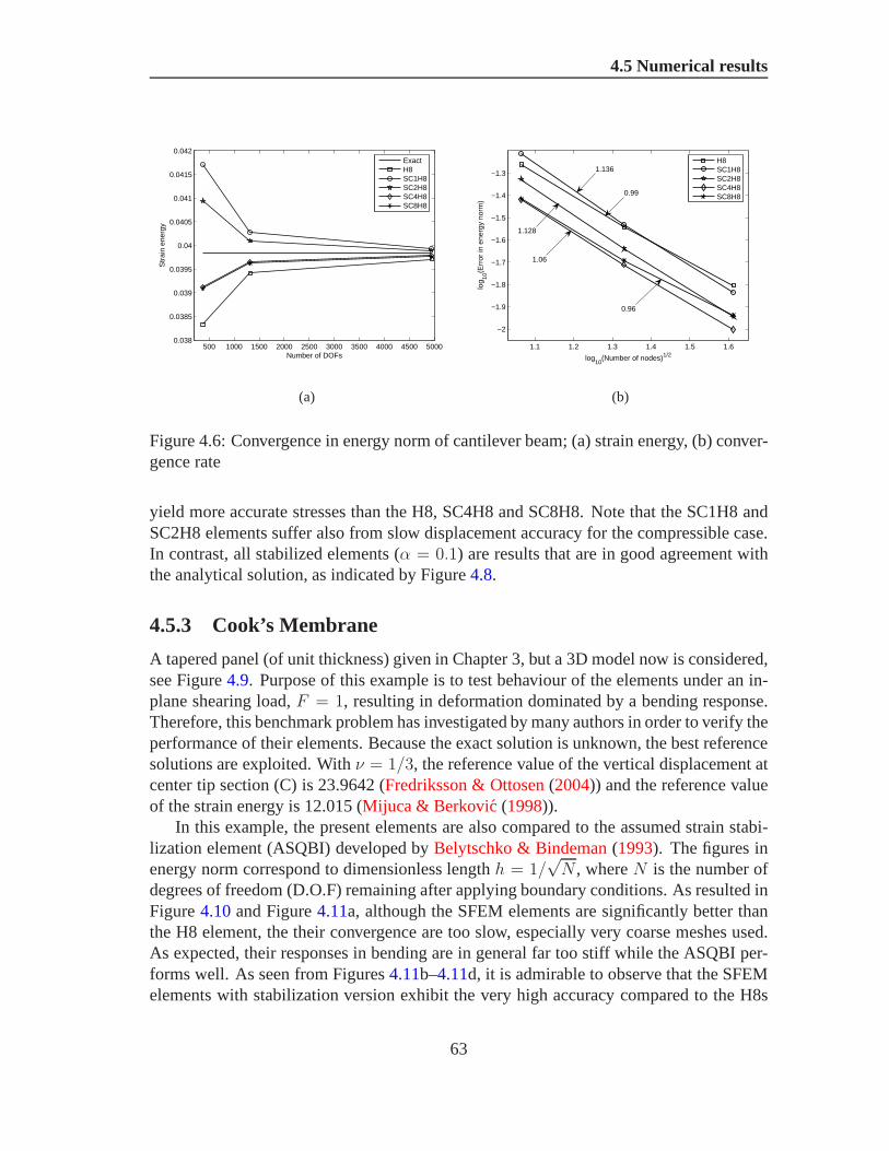
4.5 Numerical results
500 1000 1500 2000 2500 3000 3500 4000 4500 50000.038
0.0385
0.039
0.0395
0.04
0.0405
0.041
0.0415
0.042
Number of DOFs
Str
ain
ener
gyExactH8SC1H8SC2H8SC4H8SC8H8
(a)
1.1 1.2 1.3 1.4 1.5 1.6
−2
−1.9
−1.8
−1.7
−1.6
−1.5
−1.4
−1.3
log10
(Number of nodes)1/2
log 10
(Err
or in
ene
rgy
norm
)
H8SC1H8SC2H8SC4H8SC8H8
0.96
1.128
1.06
1.136
0.99
(b)
Figure 4.6: Convergence in energy norm of cantilever beam; (a) strain energy, (b) conver-gence rate
yield more accurate stresses than the H8, SC4H8 and SC8H8. Note that the SC1H8 andSC2H8 elements suffer also from slow displacement accuracyfor the compressible case.In contrast, all stabilized elements (α = 0.1) are results that are in good agreement withthe analytical solution, as indicated by Figure4.8.
4.5.3 Cook’s Membrane
A tapered panel (of unit thickness) given in Chapter 3, but a 3D model now is considered,see Figure4.9. Purpose of this example is to test behaviour of the elementsunder an in-plane shearing load,F = 1, resulting in deformation dominated by a bending response.Therefore, this benchmark problem has investigated by manyauthors in order to verify theperformance of their elements. Because the exact solution is unknown, the best referencesolutions are exploited. Withν = 1/3, the reference value of the vertical displacement atcenter tip section (C) is 23.9642 (Fredriksson & Ottosen(2004)) and the reference valueof the strain energy is 12.015 (Mijuca & Berkovic (1998)).
In this example, the present elements are also compared to the assumed strain stabi-lization element (ASQBI) developed byBelytschko & Bindeman(1993). The figures inenergy norm correspond to dimensionless lengthh = 1/
√N , whereN is the number of
degrees of freedom (D.O.F) remaining after applying boundary conditions. As resulted inFigure4.10and Figure4.11a, although the SFEM elements are significantly better thanthe H8 element, the their convergence are too slow, especially very coarse meshes used.As expected, their responses in bending are in general far too stiff while the ASQBI per-forms well. As seen from Figures4.11b–4.11d, it is admirable to observe that the SFEMelements with stabilization version exhibit the very high accuracy compared to the H8s
63

4.5 Numerical results
0 1 2 3 4 5 6 7 8−2
−1.5
−1
−0.5
0
0.5
1
1.5
2
x 10−3
x (y=0)
Ver
tical
dis
plac
emen
t v
ExactH8SC1H8SC2H8SC4H8SC8H8
(a)
−2 −1.5 −1 −0.5 0 0.5 1 1.5 2−400
−300
−200
−100
0
100
200
300
400
x=L/2N
orm
al s
tres
s
ExactH8SC1H8SC2H8SC4H8SC8H8
(b)
−2 −1.5 −1 −0.5 0 0.5 1 1.5 2−100
−90
−80
−70
−60
−50
−40
−30
−20
−10
0
x=L/2
She
ar s
tres
s
ExactH8SC1H8SC2H8SC4H8SC8H8
(c)
Figure 4.7: Solutions of 3D cantilever in near incompressibility : (a) vertical displacement(0 ≤ x ≤ L, y=0); (b) Normal stress (−D/2 ≤ y ≤ D/2); (c) Shear stress (−D/2 ≤y ≤ D/2)
64

4.5 Numerical results
0 1 2 3 4 5 6 7 8
−3
−2
−1
0
x 10−4
x (y=0)
Ver
tical
dis
plac
emen
t v
ExactH8sSC4H8sSC8H8s
(a)
−2 −1.5 −1 −0.5 0 0.5 1 1.5 2−400
−300
−200
−100
0
100
200
300
400
x=L/2N
orm
al s
tres
s
ExactH8sSC4H8sSC8H8s
(b)
−2 −1.5 −1 −0.5 0 0.5 1 1.5 2−100
−90
−80
−70
−60
−50
−40
−30
−20
−10
0
x=L/2
She
ar s
tres
s
ExactH8sSC4H8sSC8H8s
(c)
Figure 4.8: Solutions of 3D cantilever in near incompressibility using stabilization tech-nique: (a) vertical displacement (0 ≤ x ≤ L, y=0); (b) Normal stress (−D/2 ≤ y ≤D/2); (c) Shear stress (−D/2 ≤ y ≤ D/2)
65

4.5 Numerical results
and ASQBI. However, the stabilization approach for this problem do not make to improvethe convergence rate of the SFEM elements. It is noted that for this problem the marginaldifference between the SC4H8s and SC8H8s is addressed.
Figure 4.9: 3D Cook’s membrane model and coarse mesh
5 10 15 20 25 305
6
7
8
9
10
11
12
13
14
15
Elements per edge
Str
ain
ener
gy
Ref sol.H8ASQBISC1H8SC2H8SC4H8SC8H8
(a)
−2 −1.8 −1.6 −1.4 −1.2 −1 −0.8−1
−0.8
−0.6
−0.4
−0.2
0
0.2
0.4
0.6
h
log 10
(Err
or in
ene
rgy
norm
)
H8ASQBISC1H8SC2H8SC4H8SC8H81.08
0.925
0.823
0.805(SC4H8)
0.802(SC8H8)
0.773
(b)
Figure 4.10: The convergence in energy norm; (a) Strain energy, (b) Convergence rate
4.5.4 A 3D squared hole plate
Consider the 3D squared hole plate subjected to the surface tractionq as given by Fig-ure 4.16. Due to its symmetry, a quarter of the domain is modelled. Thenumericalparameters are as follows:q = 1, a = 1, t = 1, E = 1, ν = 0.3. Figure4.13plots defor-mation of domain after applying surface load. The estimatedstrain energy derived fromthe procedure of Richardson’s extrapolation byCugnon(2000) is 6.203121186.
66

4.5 Numerical results
0 5 10 15 20 25 30
12
14
16
18
20
22
24
Elements per edge
Cen
tral
tip
disp
lace
men
t
Ref sol.H8ASQBISC4H8SC8H8
(a)
5 10 15 20 25 3016
17
18
19
20
21
22
23
24
Elements per edge
Cen
tral
tip
disp
lace
men
t
Ref sol.H8sASQBISC4H8sSC8H8s
(b)
5 10 15 20 25 308
8.5
9
9.5
10
10.5
11
11.5
12
Elements per edge
Str
ain
ener
gy
Ref sol.H8sASQBISC4H8sSC8H8s
(c)
−1.8 −1.6 −1.4 −1.2 −1 −0.8
−0.8
−0.6
−0.4
−0.2
0
0.2
0.4
h
log 10
(Err
or in
ene
rgy
norm
)
H8s ASQBI SC4H8s SC8H8s 0.925
0.702
0.823
0.692
(d)
Figure 4.11: The convergence of tip displacement: (a) Without stabilization, (b) Withstabilization (α = 0.1); and (c), (d) Strain energy and convergence rate with stabilization(α = 0.1), respectively
67

4.5 Numerical results
As mentioned in Chapter 3, a stress singularity exists at there-entrant corner. Thepercentage of relative energy error is obtained in Table4.2. The convergence of the strainenergy is displayed on Figure4.14a, and the convergence rates are given in Figure4.14b.It is seen that the SFEM elements are more accurate than the standard FEM. Additionally,the SC1H8 provides the optimum rate for this singular problem.
Table 4.2: The results on percentage of relative error in energy norm of 3D L-shape
Mesh No. D.O.F H8 SC1H8 SC2H8 SC4H8 SC8H8
1 171 34.10 32.07 12.18 28.44 29.212 925 20.43 13.45 9.75 17.12 17.493 5913 12.01 6.45 6.37 10.24 10.424 11011 10.15 5.14 5.53 8.71 8.85
Figure 4.12: Squared hole structure under traction and 3D L-shape model
4.5.5 Finite plate with two circular holes
Figure4.15a illustrates a finite plate with two holes of radiusr = 0.2m subjected to aninternal pressurep = 5kPa. Due to its symmetry, only the below left quadrant of the plateis modeled. The material properties are: Young’s modulusE = 2.1× 10¹¹Pa, poisson’sratio ν = 0.3. The analytical solution is unknown. In order to estimate the reliability of
68

4.5 Numerical results
Figure 4.13: An illustration for deformation of 3D L-shape model
103
104
5.4
5.6
5.8
6
6.2
6.4
6.6
6.8
Number of DOF
Str
ain
ener
gy
RefH8SC1H8SC2H8SC4H8SC8H8
(a)
−2 −1.9 −1.8 −1.7 −1.6 −1.5 −1.4 −1.3 −1.2 −1.1
−0.7
−0.6
−0.5
−0.4
−0.3
−0.2
−0.1
0
0.1
h
log 10
(Err
or in
ene
rgy
norm
)
H8SC1H8SC2H8SC4H8SC8H8
0.386
0.608
0.602
0.607
1.029
(b)
Figure 4.14: The convergence in energy norm for the 3D squarehole problem; (a) Strainenergy, (b) Convergence rate
69

4.6 Concluding Remarks
the present method, the procedure of Richardson’s extrapolation (Richardson(1910)) isused for the SFEM solution and find that the best estimated strain energy obtained by theSC1H8 element is0.61026×10−5. The relative error and convergence rates are evaluatedbased on this estimated global energy. The convergence of energy norm is plotted inFigure4.17. It is clear that superior accuracy of the SFEM elements overthe standard H8element is observed.
(a)
0
0.2
0.4
0.6
0.8
0
0.2
0.4
0.6
0
0.1
0.2
(b)
Figure 4.15: Finite plate with two circular holes and coarsemesh; (a) Model, (b) Mesh of768 eight-node hexahedral elements
4.6 Concluding Remarks
This chapter formulated new 8 noded hexahedral elements based on the smoothed finiteelement method (SFEM) with various numbers of subcells. These elements are coinedSCkH8 wherek is the number of subcells. Low numbers of subcells lead to higher stressaccuracy but instabilities; high numbers yield lower stress accuracy but are always stable.
A stabilization procedure is proposed where the stiffness matrix is written as a linearcombination of the one subcell element and the four or eight subcell element, resulting inhigher dual (stress) accuracy and the disappearance of zeroenergy modes.
For the element with highly curved boundaries, a modified volume averaging tech-nique is proposed to replace the boundary averaging commonly used in SFEM (see also
70

4.6 Concluding Remarks
Table 4.3: The results on percentage of relative error in energy norm of finite plate withtwo holes
Mesh No. N H8SFEM
SC1H8 SC2H8 SC4H8 SC8H81 263 24.52 14.04 19.71 23.02 23.122 908 13.35 7.63 9.98 12.05 12.293 3350 7.38 3.77 5.15 6.23 6.704 12842 4.51 1.82 2.63 3.19 4.04
00.1
0.20.3
0.40.5
0.60.7
0.80.9 −0.15
−0.1−0.05
0
0
0.1
0.2
0.3
0.4
0.5
Figure 4.16: An illustration of deformation of the finite plate
0 2000 4000 6000 8000 10000 120005.7
5.75
5.8
5.85
5.9
5.95
6
6.05
6.1
6.15x 10
−6
Number of DOF
Str
ain
ener
gy
RefH8SC1H8SC2H8SC4H8SC8H8
(a)
−2.1 −2 −1.9 −1.8 −1.7 −1.6 −1.5 −1.4 −1.3 −1.2
−4.2
−4
−3.8
−3.6
−3.4
−3.2
−3
h
log 10
(Err
or in
ene
rgy
norm
)
H8SC1H8SC2H8SC4H8SC8H8
0.9
0.874
1.054
1.033
1.016
(b)
Figure 4.17: The convergence in energy norm; (a) Strain energy, (b) Convergence rate
71

4.6 Concluding Remarks
the seminal work ofStolle & Smith(2004)).
• All the SCkH8 elements always pass the patch test, even for distorted meshes.
• Except for the SC1H8 and SC2H8 elements that exhibit zero energy modes, allother smoothed elements tested are rank sufficient.
• For all examples treated, the proposed elements provide more accuracy than theFEM brick elements and are insensitive to volumetric locking when suitably stabi-lized.
• The SC4H8 (without stabilization) and the SC4H8s (with stabilization) seem to bethe best candidates for practical applications since they are both stable and accurate.
• The theoretical bases associated with the stabilization parameter need to be furtherinvestigated.
Based on the SFEM formulation coupling with partition of unity enrichment proposedby Bordaset al. (2008a) for two-dimensional crack, it will be interesting to mention howthe present SFEM can improve current extended finite elements for three-dimensionalfracture mechanics. Further studies on the behaviour of themethod for distorted meshesare required to fully assess the performance of the proposedelements. Additionally, morecomplex problems with variable thickness should be examined.
72

Chapter 5
A smoothed finite element method forplate analysis
5.1 Introduction
Plate structures play an important role in science and engineering fields. There are twodifferent plate theories, the Kirchhoff plate and the Mindlin-Reissner plate theory. Kirch-hoff plates are only applicable for thin structures where shear stresses in the plate canbe ignored. Moreover, Kirchhoff plate elements requireC1 continuous shape functions(Sander(1969); Debongnie(2003)). Mindlin-Reissner plates take shear effects into ac-count. An advantage of the Mindlin-Reissner model over the biharmonic plate modelis that the energy involves only first derivatives of the unknowns and so conforming fi-nite element approximations require only the use ofC0 shape functions instead of therequiredC1 shape functions for the biharmonic model. However, Mindlin-Reissner plateelements exhibit a phenomenon called shear locking when thethickness of the plate tendsto zero. Shear locking results in incorrect transverse forces under bending. When linearfinite element shape functions are used, the shear angle is linear within an element whilethe contribution of the displacement is only constant. The linear contribution of the rota-tion cannot be ”balanced” by a contribution from the displacement. Hence, the Kirchhoffconstraintw,x + βy = 0, w,y + βx = 0 is not fulfilled in the entire element any more.Typically, when shear locking occurs, there are large oscillating shear/transverse forcesand hence a simple smoothing procedure can drastically improve the results. In order toavoid this drawback, various improvements of formulationsas well as numerical tech-niques have been used, such as the reduced and selective integration elements (Hugheset al. (1977, 1978); Zienkiewiczet al. (1971)), equilibrium elements (Fraeijs de Veubeke& Sander(1968); Fraeijs De Veubekeet al. (1972); Sander(1969); Beckers(1972)),mixed formulation/hybrid elements byLee & Pian(1978); Lee & Wong(1982); Nguyen& Nguyen-Dang(2006); Nguyen-Dang(1980b); Nguyen-Dang & Tran(2004); Pian &Tong(1969), the Assumed Natural Strain (ANS) method (Bathe & Dvorkin(1985, 1986);Dvorkin & Bathe (1994); Hughes & Tezduyar(1981)) and Enhanced Assumed Strain
73

5.2 Meshfree methods and integration constraints
(EAS) method (Andelfinger & Ramm(1993); Simo & Rifai (1990)). Many improvedversions of plate elements have been developed and can be found in the textbooks (Bathe(1996); Zienkiewicz & Taylor (2000)). Alternative methods of stabilization approachsuch as given inGruttmann & Wagner(2004), Kouhia(2007). Of course the referencesmentioned above are by no means exhaustive.
In this chapter, improved plate elements based on the MITC4 element in which thesmoothing curvature technique (Chenet al. (2001)) is combined are presented. An in-troduction of a strain smoothing operation to the finite elements also has obtained byLiuet al.(2007a). It will be shown by numerical experiments that present method is faster andmore accurate than the original MITC4 element, at least for all examples tested. More-over, due to the integration technique, the element promises to be more accurate especiallyfor distorted meshes. Also present element is free of shear locking in limitation of thinplate.
5.2 Meshfree methods and integration constraints
In mesh-free methods based on nodal integration for Mindlin–Reissner plates, conver-gence requires fulfilling bending exactness (BE) and thus requires the following bendingintegration constraint (IC) to be satisfied, seeWang & Chen(2004)
∫
Ω
BbI(x)dΩ =
∫
Γ
EI(x)dΓ (5.1)
whereBI is the standard gradient matrix
BbI =
0 0 NI,x
0 −NI,y 00 −NI,x NI,y
, EI =
0 0 NInx
0 −NIny 00 −NInx NIny
(5.2)
The IC criterion comes from the equilibrium of the internal and external forces of theGalerkin approximation assuming pure bending. This is similar to the consistency withthe pure bending deformation in the constant moment patch test in FEM.
The basic idea is to couple the MITC element with the curvature smoothing method(CSM). Therefore, smoothing cells are constructed that do not necessarily have to becoincident with the finite elements. The integration is carried out either on the elementsthemselves, or over the smoothing cells that form a partition of the elements. The CSMis employed on each smoothing cell to normalize the local curvature and to calculate thebending stiffness matrix. The shear strains are obtained with independent interpolationfunctions as in the MITC element. Result of this work is givenby Nguyen-Xuanet al.(2008b) in detail.
74

5.3 A formulation for four-node plate element
5.3 A formulation for four-node plate element
Introducing Equation (2.70) for the curvature of the plate and applying the divergencetheorem, we obtain
κhij(xC) =
1
2AC
∫
ΩC
(∂θh
i
∂xj+
∂θhj
∂xi
)dΩ =
1
2AC
∫
ΓC
(θhi nj + θh
j ni)dΓ (5.3)
Next, we consider an arbitrary smoothing cell,ΩC illustrated in Figure3.1with boundary
ΓC =nb⋃
b=1
ΓbC , whereΓb
C is the boundary segment ofΩC , andnb is the total number of
edges of each smoothing cell. The relationship between the smoothed curvature field andthe nodal displacement is written by
κh = BbCq (5.4)
The smoothed element bending stiffness matrix is obtained by
Kb =
∫
Ωe
(BbC)TDbBb
CdΩ =
nc∑
C=1
(BbC)T (xC)DbBb
C(xC)AC (5.5)
wherenc is the number of smoothing cells of the element, see Figure3.2.Here, the integrands are constant over eachΩC and the non-local curvature displacementmatrix reads
BbCI(xC) =
1
AC
∫
ΓC
0 0 NInx
0 −NIny 00 −NInx NIny
dΓ (5.6)
We use Gauss quadrature to evaluate (5.6) with one integration point over each line seg-mentΓb
C :
BbCI(xC) =
1
AC
nb∑
b=1
0 0 NI(x
Gb )nx
0 −NI(xGb )ny 0
0 −NI(xGb )nx NI(x
Gb )ny
lCb (5.7)
wherexGb andlCb are the midpoint (Gauss point) and the length ofΓC
b , respectively.The smoothed curvatures lead to high flexibility such as arbitrary polygonal elements (Daiet al. (2007)), and a slight reduction in computational cost. The element is subdividedinto nc non-overlapping sub-domains also called smoothingcells (Liu et al. (2007a)).Figure3.2 illustrates different smoothing cells for nc = 1, 2, 3 and 4 corresponding to1-subcell, 2-subcell, 3-subcell and 4-subcell methods. The curvature is smoothed overeach sub-cell. The values of the shape functions are indicated at the corner nodes inFigure3.2in the format(N1, N2, N3, N4). The values of the non-mapped shape functionsat the integration nodes are determined based on the linear interpolation of shape functionsalong boundaries of the element or the smoothing cells, e.g.Liu et al. (2007a).
75

5.4 Numerical results
Therefore the element stiffness matrix in (2.21) can be modified as follows:
K = Kb + Ks =nc∑
C=1
(BbC)TDbBb
CAC +
∫
Ωe
(Bs)TDsBsdΩ (5.8)
It can be seen that a reduced integration on the shear termKs is necessary to avoid shearlocking as the thickness of the plate tends to zero. We will denote these elements bySC1Q4, SC2Q4, SC3Q4 and SC4Q4 corresponding to subdivisioninto nc =1, 2, 3 and4 smoothing cells, Figure3.2. However, we will show that these elements fail the patchtest and they exhibit an instability due to rank deficiency. Therefore, we employ a mixedinterpolation as in the MITC4 element and use independent interpolation fields in thenatural coordinate system (Bathe & Dvorkin(1985)) for the approximation of the shearstrains: [
γx
γy
]= J−1
[γξ
γη
](5.9)
where
γξ =1
2[(1− η)γB
ξ + (1 + η)γDξ ], γη =
1
2[(1− ξ)γA
η + (1 + ξ)γCη ] (5.10)
whereJ is the Jacobian matrix and the midside nodes A, B, C, D are shown in Figure2.2.PresentingγB
ξ , γDξ and γA
η , γCη based on the discretized fieldsuh, we obtain the shear
matrix:
BsI = J−1
[NI,ξ −b12
I NI,ξ b11I NI,ξ
NI,η −b22I NI,η b21
I NI,η
](5.11)
whereb11I = ξIx
M,ξ , b12
I = ξIyM,ξ , b21
I = ηIxL,η, b22
I = ηIyL,η (5.12)
with ξI ∈ −1, 1, 1,−1, ηI ∈ −1,−1, 1, 1 and(I, M, L) ∈ (1, B, A); (2, B, C);(3, D, C); (4, D, A). Note that the shear termKs is still computed by2 × 2 Gaussquadrature while the element bending stiffnessKb in Equation (2.44) is replaced by thesmoothed curvature technique on each smoothing cell of the element.
5.4 Numerical results
We will test our new element for different numbers of smoothing cells and call our elementMISCk (Mixed Interpolation and Smoothed Curvatures) with k∈ 1, 2, 3, 4 smoothingcells for the bending terms. For instance, the MISC1 elementis the element with onlyone smoothing cell to integrate the bending part of the element stiffness matrix. We willcompare our results to the results obtained with the reduced/selective integrated quadri-lateral element (Q4-R), the MITC4 element and with several other 4-node elements in theliteratures such as
CRB1 and CRB2 – The coupled resultants bending associated with the incompatiblemodes in mixed plate bending formulation byWeissman & Taylor(1990).
76

5.4 Numerical results
S4R – The element is commercially available byAbaqus(2004).DKQ – The Discrete Kirchhoff Quadrilateral element developed byBatoz & Tahar
(1982).G/W – A stabilized one-point integrated quadrilateral Reissner-Mindlin plate element
presented byGruttmann & Wagner(2004).
5.4.1 Patch test
The patch test was introduced by Bruce Irons and Bazeley (seeBazeleyet al. (1965)) tocheck the convergence of finite elements. It is checked if theelement is able to reproducea constant distribution of all quantities for arbitrary meshes. It is important that oneelement is completely surrounded by neighboring elements in order to test if a rigid bodymotion is modelled correctly, Figure5.1. The boundary deflection is assumed to bew =12(1+x+2y+x2+xy+y2) (Chen & Cheung(2000)). The results are shown in Table5.1.
While the MITC4 element and the MISCk elements pass the patchtest, the Q4-R elementand the SC1Q4, SC2Q4, SC3Q4, SC4Q4 elements fail the patch test. Note that also thefully integrated Q4 element (on both the bending and the shear terms) does not pass thepatch test.
Figure 5.1: Patch test of elements
5.4.2 Sensitivity to mesh distortion
Consider a clamped square plate subjected to a center pointF or uniform loadp shownin Figure5.2. The geometry parameters and the Poisson’s ratio are: length L, thicknesst, andν = 0.3. Due to its symmetry, only a quarter (lower – left) of the plate is modelledwith a mesh of 8× 8 elements. To study the effect of mesh distortion on the results,interior nodes are moved by an irregularity factors. The coordinates of interior nodes is
77

5.4 Numerical results
Table 5.1: Patch test
Element w5 θx5 θy5 mx5 my5 mxy5
Q4-R 0.5440 1.0358 -0.676 — — —SC1Q4 0.5431 1.0568 -0.7314 — — —SC2Q4 0.5439 1.0404 -0.6767 — — —SC3Q4 0.5440 1.0396 -0.6784 — — —SC4Q4 0.5439 1.0390 -0.6804 — — —MITC4 0.5414 1.04 -0.55 -0.01111 -0.01111 -0.00333MISC1 0.5414 1.04 -0.55 -0.01111 -0.01111 -0.00333MISC2 0.5414 1.04 -0.55 -0.01111 -0.01111 -0.00333MISC3 0.5414 1.04 -0.55 -0.01111 -0.01111 -0.00333MISC4 0.5414 1.04 -0.55 -0.01111 -0.01111 -0.00333Exact 0.5414 1.04 -0.55 -0.01111 -0.01111 -0.00333
— no constant moments
perturbed as follows (Liu et al. (2007a)):
x′ = x + rcs∆xy′ = y + rcs∆y
(5.13)
whererc is a generated random number given values between -1.0 and 1.0, s ∈ [0, 0.5] isused to control theshapes of the distorted elements and∆x, ∆y are initial regular elementsizes in thex–andy–directions, respectively.
For the concentrated center point loadF , the influence of the mesh distortion on thecenter deflection is given in Figure5.3 for a thickness ratio of (t/L = 0.01 and0.001).The results of our presented method are more accurate than those of the Q4-R elementand the MITC4 element, especially for extremely distorted meshes. Here, the MISC1element gives the best result. However, this element contains two zero-energy modes. Insimple problems, these hourglass modes can be automatically eliminated by the boundaryconditions. However, this is not in general the case. Otherwise, the MISC2, MISC3 andMISC4 elements retain a sufficient rank of the element stiffness matrix and give excellentresults.
Let us consider a thin plate with(t/L = 0.001) under uniform load as shown Fig-ure 5.2a. The numerical results of the central deflections are shownin Table 5.2 andFigure5.4 and compared to other elements. Overall, it can be seen that the MISCk ele-ments give more accurate results than the other elements, especially for distorted meshes.
5.4.3 Square plate subjected to a uniform load or a point load
Figure 5.2a and Figure5.5 are the model of a square plate with clamped and simplysupported boundary conditions, respectively, subjected to a uniform loadp = 1 or a
78

5.4 Numerical results
(a) (b)
(c) (d)
Figure 5.2: Effect of mesh distortion for a clamped square plate: (a) clamped plate model;(b) s = 0.3; (c) s = 0.4; and (d)s = 0.5
79

5.4 Numerical results
0 0.1 0.2 0.3 0.4 0.50.84
0.86
0.88
0.9
0.92
0.94
0.96
0.98
1
1.02
Distorsion s
Nor
mal
ized
def
lect
ion
wc
Exact solu.Q4−RMITC4MISC1MISC2MISC3MISC4
(a)
0 0.1 0.2 0.3 0.4 0.50.5
0.55
0.6
0.65
0.7
0.75
0.8
0.85
0.9
0.95
1
Distorsion s
Nor
mal
ized
def
lect
ion
wc
Exact solu.Q4−RMITC4MISC1MISC2MISC3MISC4
(b)
Figure 5.3: The normalized center deflection with influence of mesh distortion for aclamped square plate subjected to a concentrated load: a) t/L=0.01, b) t/L=0.001
−1.5 −1 −0.5 0 0.5 1 1.50.08
0.1
0.12
0.14
0.16
0.18
0.2
0.22
0.24
0.26
Distortion parameter
Cen
tral
def
lect
ion
wc/(
pL4 /1
00D
)
CRB1CRB2S1S4RDKQMITC4MISC1MISC2MISC3MISC4Exact
Figure 5.4: Comparison of other elements through the centerdeflection with mesh distor-tion
80

5.4 Numerical results
Table 5.2: The central deflectionwc/(pL4/100D), D = Et3/12(1 − ν2) with mesh dis-tortion for thin clamped plate subjected to uniform loadp
s -1.249 -1.00 -0.5 0.00 0.5 1.00 1.249
CRB1 0.1381 0.1390 0.1247 0.1212 0.1347 0.1347 0.1249CRB2 0.2423 0.1935 0.1284 0.1212 0.1331 0.1647 0.1947Q4-R 0.1105 0.1160 0.1209 0.1211 0.1165 0.1059 0.0975S4R 0.1337 0.1369 0.1354 0.1295 0.1234 0.1192 0.1180DKQ 0.1694 0.1658 0.1543 0.1460 0.1418 0.1427 0.1398
MITC4 0.0973 0.1032 0.1133 0.1211 0.1245 0.1189 0.1087MISC1 0.1187 0.1198 0.1241 0.1302 0.1361 0.1377 0.1347MISC2 0.1151 0.1164 0.1207 0.1266 0.1323 0.1331 0.1287MISC3 0.1126 0.1144 0.1189 0.1249 0.1305 0.1309 0.1260MISC4 0.1113 0.1130 0.1174 0.1233 0.1287 0.1288 0.1227
Exact solu. 0.1265 0.1265 0.1265 0.1265 0.1265 0.1265 0.1265
Figure 5.5: A simply supported square plate subjected to a point load or a uniform load
81

5.4 Numerical results
central loadF = 16.3527. The material parameters are given by Young’s modulusE =1092000 and Poisson’s ratioν = 0.3. Uniform meshes withN = 2, 4, 8, 16, 32 areused and symmetry conditions are exploited. For a clamped case, Figure5.6 illustratesthe convergence of the normalized deflection and the normalized moment at the centerversus the mesh densityN for a relationt/L = 0.01. Even for very coarse meshes,the deflection tends to the exact solution. For the finest mesh, the displacement slightly(.06%) exceeds the value of the exact solution. The bending momentconverges to theanalytical value. The rate of convergence in the energy normis presented in Figure5.7and is for all elements equal to1.1 but the MISCk elements are more accurate than theMITC4 element.
1 1.5 2 2.5 3 3.5 4 4.5 50.95
0.96
0.97
0.98
0.99
1
1.01
1.02
1.03
Mesh NxN
Nor
mal
ized
def
lect
ion
wc
Exact solu.MITC4MISC1MISC2MISC3MISC4
(a)
1 1.5 2 2.5 3 3.5 4 4.5 50.8
0.85
0.9
0.95
1
Mesh NxN
Nor
mal
ized
cen
tral
mom
ent
Exact solu.MITC4MISC1MISC2MISC3MISC4
(b)
Figure 5.6: Normalized deflection and moment at center of clamped square plate sub-jected to uniform load
Tables5.3–5.4 show the performance of the plate element compared the exactsolu-tion1 for different thickness ratios,t/L = 10−1 ∼ 10−5. No shear locking is observed.
Next we consider a sequence of distorted meshes with 25, 81, 289 and 1089 nodes asshown in Figure5.8. The numerical results in terms of the error in the central displace-ment and the strain energy are illustrated in Figure5.9. All proposed elements give stableand accurate results. Especially for coarse meshes, the MISCk elements are more accu-rate than the MITC4 element; a reason for this may be that for our finest meshes, fewerelements are distorted in comparison to coarse meshes.
Now we will test the computing time for the clamped plate analyzed above. Theprogram is compiled by a personal computer with Pentium(R)4, CPU-3.2GHz and RAM-512MB. The computational cost to set up the global stiffnessmatrix and to solve thealgebraic equations is illustrated in Figure5.10. The MISCk elements and the MITC4
1The exact value is cited fromTaylor & Auricchio (1993)
82

5.4 Numerical results
Table 5.3: Central deflectionswc/(pL4/100D) for the clamped plate subjected to uni-form load
L/t elementsMesh
2 4 8 16 32 ExactMITC4 0.1431 0.1488 0.1500 0.1504 0.1504MISC1 0.1517 0.1507 0.1505 0.1505 0.1505
10 MISC2 0.1483 0.1500 0.1503 0.1504 0.1505 0.1499MISC3 0.1467 0.1496 0.1502 0.1504 0.1504MISC4 0.1451 0.1493 0.1502 0.1504 0.1504
MITC4 0.1213 0.1253 0.1264 0.1267 0.1268MISC1 0.1304 0.1274 0.1269 0.1268 0.1268
102 MISC2 0.1269 0.1266 0.1267 0.1268 0.1268 0.1267MISC3 0.1252 0.1262 0.1266 0.1267 0.1268MISC4 0.1235 0.1258 0.1265 0.1267 0.1268
MITC4 0.1211 0.1251 0.1262 0.1264 0.1265MISC1 0.1302 0.1272 0.1267 0.1266 0.1265
103 MISC2 0.1266 0.1264 0.1265 0.1265 0.1265 0.1265MISC3 0.1249 0.1260 0.1264 0.1265 0.1265MISC4 0.1233 0.1256 0.1263 0.1265 0.1265
MITC4 0.1211 0.1251 0.1262 0.1264 0.1265MISC1 0.1302 0.1272 0.1267 0.1266 0.1265
104 MISC2 0.1266 0.1264 0.1265 0.1265 0.1265 0.1265MISC3 0.1249 0.1260 0.1264 0.1265 0.1265MISC4 0.1233 0.1256 0.1263 0.1265 0.1265
MITC4 0.1211 0.1251 0.1262 0.1264 0.1265MISC1 0.1302 0.1272 0.1267 0.1266 0.1265
105 MISC2 0.1266 0.1264 0.1265 0.1265 0.1265 0.1265MISC3 0.1249 0.1260 0.1264 0.1265 0.1265MISC4 0.1233 0.1256 0.1263 0.1265 0.1265
83

5.4 Numerical results
Table 5.4: Central momentsMc/(pL2/10) for the clamped plate subjected to uniformload
L/t elementsMesh
2 4 8 16 32 ExactMITC4 0.1898 0.2219 0.2295 0.2314 0.2318MISC1 0.2031 0.2254 0.2304 0.2316 0.2319
10 MISC2 0.1982 0.2241 0.2300 0.2315 0.2319 0.231MISC3 0.1974 0.2239 0.2300 0.2315 0.2319MISC4 0.1930 0.2228 0.2297 0.2314 0.2319
MITC4 0.1890 0.2196 0.2267 0.2285 0.2289MISC1 0.2031 0.2233 0.2277 0.2287 0.2290
102 MISC2 0.1976 0.2218 0.2273 0.2286 0.2290 0.2291MISC3 0.1974 0.2217 0.2273 0.2286 0.2290MISC4 0.1923 0.2205 0.2270 0.2286 0.2290
MITC4 0.1890 0.2196 0.2267 0.2285 0.2289MISC1 0.2031 0.2233 0.2276 0.2287 0.2290
103 MISC2 0.1976 0.2218 0.2273 0.2286 0.2289 0.2291MISC3 0.1974 0.2217 0.2272 0.2286 0.2289MISC4 0.1923 0.2205 0.2269 0.2285 0.2289
MITC4 0.1890 0.2196 0.2267 0.2285 0.2289MISC1 0.2031 0.2233 0.2276 0.2287 0.2290
104 MISC2 0.1976 0.2218 0.2273 0.2286 0.2289 0.2291MISC3 0.1974 0.2217 0.2272 0.2286 0.2289MISC4 0.1923 0.2205 0.2269 0.2285 0.2289
MITC4 0.1890 0.2196 0.2267 0.2285 0.2289MISC1 0.2031 0.2233 0.2276 0.2287 0.2290
105 MISC2 0.1976 0.2218 0.2273 0.2286 0.2289 0.2291MISC3 0.1974 0.2217 0.2272 0.2286 0.2289MISC4 0.1923 0.2205 0.2269 0.2285 0.2289
84

5.4 Numerical results
0.7 0.8 0.9 1 1.1 1.2 1.3 1.4 1.5 1.60.2
0.3
0.4
0.5
0.6
0.7
0.8
0.9
1
1.1
1.2
log10
(Number of nodes)1/2
log 10
(Err
or in
ene
rgy
norm
)
MITC4MISC1MISC2MISC3MISC4
Figure 5.7: Rate of convergence in energy norm versus with number of nodes for clampedsquare plate subjected to uniform load
element give nearly the same CPU time for coarse meshes wherethe MISCk elements aremore accurate. From the plots, we can conjecture that, in thelimit where the numbers ofdegrees of freedom tends to infinity, the MITC4 element is computationally more expen-sive than the MISCk element, and the MISCk elements are generally more accurate. Thelower computational cost comes from the fact that no computation of the Jacobian matrixis necessary for the MISCk elements while the MITC4 element needs to determine theJacobian determinant, the inverse of the Jacobian matrix (transformation of two coordi-nates; global coordinate and local coordinate) and then thestiffness matrix is calculatedby 2× 2 Gauss points. Previously, the same tendency was observed for the standard (Q4element).
For a simply supported plate subjected to central concentrate load, the same tendenciesas described above are observed. Exemplarily, we will show the results of the normalizeddeflection in Figure5.11a for the uniform meshes and in Figure5.11b for the distortedmeshes illustrated in Figure5.8.
The numerical results for a simply supported plate subjected to a uniform load arepresented in Tables5.5–5.6and Figures5.12– 5.13for a regular mesh. We note that theMISCk elements are more accurate than the MITC4 element but show the same conver-gence rate. We also see that no shear locking occurs with decreasing thickness. Also,for all elements presented, the displacement results do notseem to be influenced by thevalue of the thickness ratio, at least in the ranget/L ∈ [10−3, 10−5]. The moments remainaccurate throughout the range of thickness ratios that we considered.
85

5.4 Numerical results
(a) (b)
(c) (d)
Figure 5.8: Analysis of clamped plate with irregular elements: (a) 25; (b)64; (c) 256; and(d) 1024
86

5.4 Numerical results
0 5 10 15 20 25 30 35−4
−3.5
−3
−2.5
−2
−1.5
−1
−0.5
0
0.5
Mesh NxN
% e
rror
for
cent
ral d
efle
ctio
n w
c
MITC4MISC1MISC2MISC3MISC4
(a)
0 5 10 15 20 25 30 35−8
−7
−6
−5
−4
−3
−2
−1
0
Mesh NxN
% e
rror
in s
trai
n en
ergy
MITC4MISC1MISC2MISC3MISC4
(b)
Figure 5.9: The convergence test of thin clamped plate (t/L=0.001) (with irregular ele-ments: (a) the deflection; (b) the strain energy
0 0.5 1 1.5 2 2.5 3
x 104
0
50
100
150
200
250
300
350
400
450
Degrees of freedom
CP
U ti
mes
(se
c)
MITC4MISC1MISC2MISC3MISC4
Figure 5.10: Computational cost for establishing the global stiffness matrix and solvingsystem equations of clamped plate subjected to a uniform load
87

5.4 Numerical results
0 10 20 30 40 50 600.994
0.996
0.998
1
1.002
1.004
1.006
1.008
1.01
Mesh NxN
Nor
mal
ized
def
lect
ion
at c
ente
r
Exact solu.Q4−RMITC4MISC1MISC2MISC3MISC4
(a) regular mesh
0 5 10 15 20 25 30 350.7
0.75
0.8
0.85
0.9
0.95
1
Mesh NxN
Nor
mal
ized
def
lect
ion
at c
ente
r
Exact solu.Q4−RMITC4MISC1MISC2MISC3MISC4
(b) distorted mesh
Figure 5.11: Normalized deflection at the centre of the simply supported square platesubjected to a center load
1 1.5 2 2.5 3 3.5 4 4.5 50.975
0.98
0.985
0.99
0.995
1
1.005
1.01
1.015
1.02
1.025
Index mesh N
Nor
mal
ized
def
lect
ion
w
Analytical solu.MITC4MISC1MISC2MISC3MISC4
(a)
0.5 1 1.5 2 2.5 3 3.5 4 4.5 50.85
0.9
0.95
1
1.05
Index mesh N
Nor
mal
ized
mom
ent a
t cen
tre
Analytical solu.MITC4MISC1MISC2MISC3MISC4
(b)
Figure 5.12: Normalized deflection and moment at center of simply support square platesubjected to uniform load
88

5.4 Numerical results
Table 5.5: Central deflectionswc/(pL4/100D) for the simply supported plate subjectedto uniform load
L/t elementsMesh
2 4 8 16 32 ExactMITC4 0.4190 0.4255 0.4268 0.4272 0.4273MISC1 0.4344 0.4290 0.4277 0.4274 0.4273
10 MISC2 0.4285 0.4277 0.4274 0.4273 0.4273 0.4273MISC3 0.4256 0.4270 0.4272 0.4273 0.4273MISC4 0.4227 0.4263 0.4271 0.4272 0.4273
MITC4 0.3971 0.4044 0.4059 0.4063 0.4064MISC1 0.4125 0.4079 0.4068 0.4065 0.4065
102 MISC2 0.4066 0.4066 0.4065 0.4065 0.4064 0.4064MISC3 0.4037 0.4059 0.4063 0.4064 0.4064MISC4 0.4008 0.4052 0.4062 0.4064 0.4064
MITC4 0.3969 0.4041 0.4057 0.4061 0.4062MISC1 0.4123 0.4077 0.4066 0.4063 0.4063
103 MISC2 0.4064 0.4064 0.4063 0.4062 0.4062 0.4062MISC3 0.4035 0.4057 0.4061 0.4062 0.4062MISC4 0.4006 0.4050 0.4059 0.4062 0.4062
MITC4 0.3969 0.4041 0.4057 0.4061 0.4062MISC1 0.4123 0.4077 0.4066 0.4063 0.4063
104 MISC2 0.4064 0.4064 0.4063 0.4062 0.4062 0.4062MISC3 0.4035 0.4057 0.4061 0.4062 0.4062MISC4 0.4006 0.4050 0.4059 0.4062 0.4062
MITC4 0.3969 0.4041 0.4057 0.4061 0.4062MISC1 0.4123 0.4077 0.4066 0.4063 0.4063
105 MISC2 0.4064 0.4064 0.4063 0.4062 0.4062 0.4062MISC3 0.4035 0.4057 0.4061 0.4062 0.4062MISC4 0.4006 0.4050 0.4059 0.4062 0.4062
89

5.4 Numerical results
Table 5.6: Central momentsMc/(pL2/10) for the simply supported plate subjected touniform load
L/t elementsMesh
2 4 8 16 32 ExactMITC4 0.4075 0.4612 0.4745 0.4778 0.4786MISC1 0.4232 0.4652 0.4755 0.4780 0.4787
10 MISC2 0.4172 0.4637 0.4751 0.4779 0.4786MISC3 0.4169 0.4637 0.4751 0.4779 0.4786MISC4 0.4113 0.4622 0.4747 0.4778 0.4786
MITC4 0.4075 0.4612 0.4745 0.4778 0.4786MISC1 0.4232 0.4652 0.4755 0.4780 0.4787
102 MISC2 0.4171 0.4637 0.4751 0.4779 0.4786MISC3 0.4169 0.4636 0.4751 0.4779 0.4786MISC4 0.4113 0.4622 0.4747 0.4778 0.4786
0.4789MITC4 0.4075 0.4612 0.4745 0.4778 0.4786MISC1 0.4232 0.4652 0.4755 0.4780 0.4787
103 MISC2 0.4171 0.4637 0.4751 0.4779 0.4786MISC3 0.4169 0.4636 0.4751 0.4779 0.4786MISC4 0.4113 0.4622 0.4747 0.4778 0.4786
MITC4 0.4075 0.4612 0.4745 0.4778 0.4786MISC1 0.4232 0.4652 0.4755 0.4780 0.4787
104 MISC2 0.4171 0.4637 0.4751 0.4779 0.4786MISC3 0.4169 0.4636 0.4751 0.4779 0.4786MISC4 0.4113 0.4622 0.4747 0.4778 0.4786
MITC4 0.4075 0.4612 0.4745 0.4778 0.4786MISC1 0.4232 0.4652 0.4755 0.4780 0.4786
105 MISC2 0.4171 0.4637 0.4751 0.4779 0.4786MISC3 0.4169 0.4636 0.4751 0.4779 0.4786MISC4 0.4113 0.4622 0.4747 0.4778 0.4786
90

5.4 Numerical results
0.7 0.8 0.9 1 1.1 1.2 1.3 1.4 1.5 1.6−1.4
−1.2
−1
−0.8
−0.6
−0.4
−0.2
0
log10
(Number of nodes)1/2
log 10
(Err
or in
ene
rgy
norm
)
MITC4MISC1MISC2MISC3MISC4
1.243
1.253
1.232
1.264
1.292
Figure 5.13: Rate of convergence in energy norm for simply supported square plate sub-jected to uniform load
5.4.4 Skew plate subjected to a uniform load
5.4.4.1 Razzaque’s skew plate model.
Let us consider a rhombic plate subjected to a uniform loadp = 1 as shown in Figure5.14a. This plate was originally studied byRazzaque(1973). Dimensions and boundaryconditions are specified in Figure5.14a, too. Geometry and material parameters are lengthL = 100, thicknesst = 0.1, Young’s modulusE = 1092000 and Poisson’s ratioν = 0.3.The results in Table5.7 show that the accuracy of the presented method is always betterthan that of the MITC4 element. Figure5.15illustrates the contribution of the von Misesstresses and the level lines for Razzaque’s skew plate with our MISC4 element.
5.4.4.2 Morley’s skew plate model.
The set-up of a skew plate is shown in Figure5.14b. This example was first studied byMorley (1963). The geometry and material parameters are lengthL = 100, thicknesst,Young’s modulusE = 1092000, Poisson’s ratioν = 0.3 and a uniform loadp = 1. Thevalues of the deflection at the central point are given in Figure 5.17 for different platethickness. The MISCk elements show remarkably good resultscompared the MITC4element. The distribution of the von Mises stresses and the level lines are illustratedin Figure5.16. It is evident that this problem has the corner singularity.An adaptiveapproach might be useful for computational reasons.
91

5.4 Numerical results
(a)
(b)
Figure 5.14: A simply supported skew plate subjected to a uniform load
0 50 100 150
0
20
40
60
80
100 graph
100
200
300
400
500
600
700
800
900
1000
(a)
0 50 100 150
0
20
40
60
80
100
level lines
(b)
Figure 5.15: A distribution of von Mises stress and level lines for Razzaque’s skew plateusing MISC4 element
92

5.4 Numerical results
Table 5.7: Central defection and moment of the Razzaque’s skew plate
Mesh MITC4 MISC1 MISC2 MISC3 MISC4
(a) Central deflectionwc/104
2×2 0.3856 0.3648 0.3741 0.3781 0.38164×4 0.6723 0.6702 0.6725 0.6725 0.67246×6 0.7357 0.7377 0.7377 0.7370 0.73648×8 0.7592 0.7615 0.7610 0.7604 0.7598
12×12 0.7765 0.7781 0.7776 0.7772 0.776916×16 0.7827 0.7838 0.7834 0.7832 0.783032×32 0.7888 0.7892 0.7891 0.7890 0.7889
Razzaque(1973) 0.7945
(b) Central momentMy/103
2×2 0.4688 0.4688 0.4688 0.4688 0.46884×4 0.8256 0.8321 0.8301 0.8284 0.82696×6 0.8976 0.9020 0.9005 0.8994 0.89848×8 0.9242 0.9272 0.9260 0.9254 0.9245
12×12 0.9439 0.9454 0.9448 0.9445 0.944216×16 0.9510 0.9518 0.9515 0.9513 0.951132×32 0.9577 0.9580 0.9579 0.9578 0.9578
Razzaque(1973) 0.9589
0 50 100 150
−40
−20
0
20
40
60
80
50
100
150
200
250
(a)
0 20 40 60 80 100 120 140 160 180
−40
−20
0
20
40
60
80
level lines
(b)
Figure 5.16: A distribution of von Mises and level lines for Morley’s skew plate usingMISC2 element
93

5.4 Numerical results
0 5 10 15 20 25 30 350.8
1
1.2
1.4
1.6
1.8
2
Index mesh NxN
Nor
mal
ized
def
lect
ion
wc
Exact solu.Q4BLDKMQARS−Q12MITC4MISC1MISC2MISC3MISC4
L/t = 1000
(a)
0 5 10 15 20 25 30 350.8
1
1.2
1.4
1.6
1.8
2
Index mesh NxN
Nor
mal
ized
def
lect
ion
wc
Exact solu.Q4BLDKMQARS−Q12MITC4MISC1MISC2MISC3MISC4
L/t=100
(b)
Figure 5.17: The convergence of the central deflectionwc for Morley plate with differentthickness/span ratio
5.4.5 Corner supported square plate
Consider a corner supported plate subjected to a uniform load p = 0.03125 with edgelengthL = 24 and thicknesst = 0.375. This example is often studied to test the existenceof spurious energy modes. The material parameters are Young’s modulusE = 430000and Poisson’s ratioν = 0.38. The shear correction factor was set to a value ofk = 1000.A symmetric model with an initial mesh of8 × 8 elements is shown in Figure5.18.Table5.8 shows the convergence of the center deflection. We note that even our rank-deficient MISC1 element gives stable and very accurate results.
We have also carried out a frequency analysis. The mass density is chosen to beρ = 0.001 and the normalized frequencies areω = ωL2(D/tρ)−1/2. The results areillustrated in Table5.9for two mesh densities (6× 6 and32× 32). It can be seen that allproposed elements give stable and accurate solutions.
5.4.6 Clamped circular plate subjected to a concentrated load
Let us consider a clamped circular plate with radiusR = 5 subjected to a point loadF = 1at the center. The material and geometric parameters are Young’s modulusE = 10.92,Poisson’s ratioν = 0.3 and the thickness of the plate is1. The analytical deflection forthis problem is
w(r) =FR2
16πD
(1− r2
R2+
2r2
R2ln
r
R− 8D
kGtR2ln
r
R
)(5.14)
A discretization of this problem with 48 elements is illustrated in Figure5.19. We ex-ploited the symmetry of the plate and modelled only one quarter. Because of the singular-
94

5.4 Numerical results
Figure 5.18: Corner supported plate subjected to uniform load
Table 5.8: The convergence of center defection for corner supported plate
Elem. per side 8 16 24 48 96
DKQ 0.11914 0.11960 0.11969 0.11974 0.11975G/W 0.11862 0.11947 0.11963 0.11973 0.11975
MITC4 0.11856 0.11946 0.11963 0.11973 0.11975MISC1 0.11873 0.11950 0.11965 0.11973 0.11975MISC2 0.11867 0.11949 0.11964 0.11973 0.11975MISC3 0.11864 0.11948 0.11963 0.11973 0.11975MISC4 0.11861 0.11947 0.11963 0.11973 0.11975Theory 0.12253
Table 5.9: Three lowest frequencies for corner supported plate
Element6× 6 mesh 32× 32 mesh
ω1 ω2 ω3 ω1 ω2 ω3
DKQ 7.117 18.750 43.998 – – –G/W 7.144 18.800 44.105 – – –
MITC4 7.135 18.795 44.010 7.036 18.652 43.163MISC1 7.136 18.799 44.011 7.075 18.661 43.553MISC2 7.141 18.800 44.065 7.075 18.661 43.555MISC3 7.143 18.800 44.092 7.075 18.661 43.556MISC4 7.145 18.800 44.119 7.076 18.661 43.557
Leissa(1969) 7.120 19.600 44.400
95
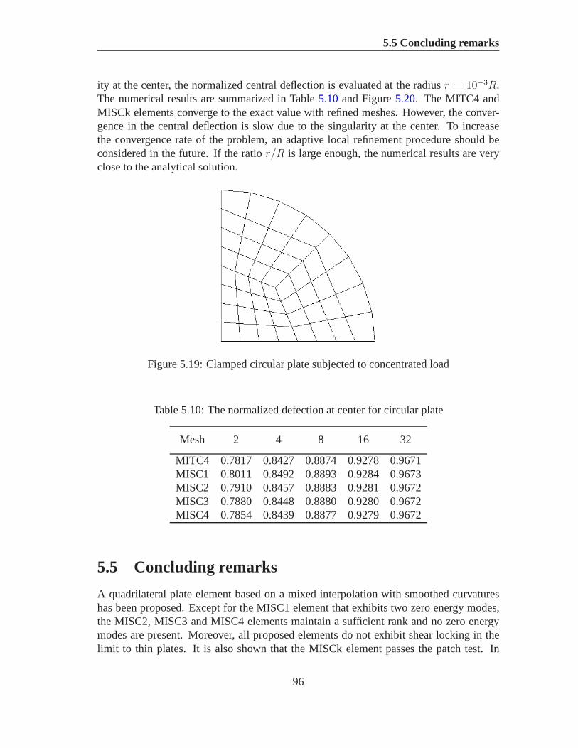
5.5 Concluding remarks
ity at the center, the normalized central deflection is evaluated at the radiusr = 10−3R.The numerical results are summarized in Table5.10and Figure5.20. The MITC4 andMISCk elements converge to the exact value with refined meshes. However, the conver-gence in the central deflection is slow due to the singularityat the center. To increasethe convergence rate of the problem, an adaptive local refinement procedure should beconsidered in the future. If the ratior/R is large enough, the numerical results are veryclose to the analytical solution.
Figure 5.19: Clamped circular plate subjected to concentrated load
Table 5.10: The normalized defection at center for circularplate
Mesh 2 4 8 16 32
MITC4 0.7817 0.8427 0.8874 0.9278 0.9671MISC1 0.8011 0.8492 0.8893 0.9284 0.9673MISC2 0.7910 0.8457 0.8883 0.9281 0.9672MISC3 0.7880 0.8448 0.8880 0.9280 0.9672MISC4 0.7854 0.8439 0.8877 0.9279 0.9672
5.5 Concluding remarks
A quadrilateral plate element based on a mixed interpolation with smoothed curvatureshas been proposed. Except for the MISC1 element that exhibits two zero energy modes,the MISC2, MISC3 and MISC4 elements maintain a sufficient rank and no zero energymodes are present. Moreover, all proposed elements do not exhibit shear locking in thelimit to thin plates. It is also shown that the MISCk element passes the patch test. In
96

5.5 Concluding remarks
0 0.2 0.4 0.6 0.8 10
0.1
0.2
0.3
0.4
0.5
0.6
0.7
0.8
0.9
Ratio r/R
Def
lect
ion
Analytical solu.MITC4MISC1MISC2MISC3MISC4
Figure 5.20: Clamped circular plate subjected to concentrated load
comparison to the well known MITC4 element, the proposed elements are more accurate1
for regular and especially for irregular meshes or coarse meshes while their computationalcost is lower.
The element with the best performance is the MISC1 element but it exhibits two zeroenergy modes. However, for the examples tested here, no instabilities were observed. Theelimination of the zero-energy modes of our MISC1 elements will be investigated in thefuture. The MISC2 element is almost of the same accuracy as the MISC1 element and itis stable but it is also slower.
Another study will concern the shear term. By replacing2 × 2 Gauss integration onthe shear term with a reduced integration with stabilization, we expect the element to beeven better suited to handle arbitrary mesh distortions.
1for all examples tested
97

Chapter 6
A stabilized smoothed finite elementmethod for free vibration analysis ofMindlin–Reissner plates
6.1 Introduction
The free vibration analysis of plate structures plays an important role in engineering appli-cations. Due to limitations of the analytical methods for practical applications, numericalmethods have become the most widely used computational toolfor plate structures. Oneof the most popular numerical approaches for analyzing vibration characteristics of theplates is the well-known Finite Element Method (FEM).
Although the finite element method provides a general and systematic technique forconstructing basis functions, a number of difficulties havestill existed in the develop-ment of plate elements based on shear deformation theories.One of which is the shearlocking phenomena as the plate thickness decreases. In order to avoid this drawback,various improvements of formulations as well as numerical techniques have been used,such as the reduced and selective integration elements (Zienkiewiczet al.(1971); Hugheset al. (1977); Hugheset al. (1978)), mixed formulation/hybrid elements byPian & Tong(1969); Lee & Pian(1978); Lee & Wong (1982), the Assumed Natural Strain (ANS)method (Hughes & Tezduyar(1981); Bathe & Dvorkin(1985, 1986); Dvorkin & Bathe(1994)) and Enhanced Assumed Strain (EAS) method (Simo & Rifai (1990)). Many im-proved versions of plate elements have been developed and can be found in the textbooks(Bathe(1996); Zienkiewicz & Taylor(2000)). In the other front of element’s technologydevelopment,Liu et al.(2007a) have recently proposed a smoothed finite element method(SFEM) by introducing a strain smoothing operation (Chenet al. (2001)) into the finiteelement formulation for two dimensional problems. Based onthe idea of the SFEM,Nguyen-Xuanet al. (2008b) formulated a plate element so-called the MISCk elementsby incorporating the curvature smoothing operation (the strain smoothing method) withthe original MITC4 element inBathe & Dvorkin(1985). The properties of the SFEM
98

6.2 A formulation for stabilized elements
are studied in detail byLiu et al. (2007b); Nguyenet al. (2007b); Nguyen-Xuanet al.(2007b). The SFEM has also been applied to dynamic problems for 2D solids (Dai & Liu(2007)).
The objective of this chapter is to further extend the MISCk elements to the free vi-bration analysis of plates of various shapes, see e. g.Nguyen-Xuan & Nguyen(2008).4-node quadrilateral elements are considered and each is subdivided into k∈ 1, 2, 4smoothing cells in the calculation of bending stiffness matrix. Shear strains are interpo-lated from the values of the covariant components of the transverse shear strains at fourmid-side points of the quadrilateral element. To improve the convergence of the elements,the issue of shear strain stabilization is also studied. Theevaluation of the shear stiffnessmatrix is done using2 × 2 Gauss quadrature points. Several numerical examples arepresented to show the accuracy, stability and effectiveness of the present elements. Wewill show by numerical experiments that the present method is faster and more accuratethan the original MITC4 element, at least for all examples tested. Moreover, due to theintegration technique, the element promises to be more accurate especially for distortedmeshes. Also the present element is free of shear locking in thin plate limit.
6.2 A formulation for stabilized elements
The application of the SFEM to plate analysis byNguyen-Xuanet al.(2008b) has resultedin the MISCk elements that use k∈ 1, 2, 4 smoothing cells as shown in Figure3.2 forthe bending strains and an independent interpolation for shear strains. The smoothingcells are created by subdividing the element.A smoothed curvature operation is recalled as
κh(xC) =
∫
Ωh
κh(x)Φ(x− xC)dΩ (6.1)
whereΦ is assumed to be a step function defined by
Φ(x− xC) =
1/AC ,x ∈ ΩC
0,x /∈ ΩC(6.2)
whereAC is the area of the smoothing cell,ΩC ⊂ Ωe ⊂ Ωh .Substituting Equation (6.2) into Equation (6.1), and applying the divergence theorem, weobtain
κhij(xC) =
1
2AC
∫
ΩC
(∇⊗ βh + βh ⊗∇
)ij
dΩ =1
2AC
∫
ΓC
(βhi nj + βh
j ni)dΓ (6.3)
whereΓC is the boundary of the smoothing cell andni, nj are the components of thenormal vector of the boundary.The discretized solutions of the problem associated with the smoothed operator are : find
99

6.2 A formulation for stabilized elements
ωh ∈ R+ and0 6= (wh, βh) ∈ Vh such as
a(βh, η) + λt(∇wh −Rhβh,∇v −Rhη) + k(wh, v) = (ωh)2ρt(wh, v)
+1
12ρt3(βh, η), ∀(v, η) ∈ V
h0
(6.4)
wherea(., .) is a “smoothed” bilinear form:
a(βh, η) =
ne∑
e=1
nc∑
ic=1
∫
Ωeic
κic(βh) : Db : κic(η)dΩe
ic (6.5)
and
κic =1
Aic
∫
Ωeic
κ(x)dΩeic andAe =
nc∑
ic=1
Aic (6.6)
with Aic is the area of theicth smoothing cell of the element,Ωeic ≡ ΩC .
We thus point out a modified method on the bending terms by the smoothed operator whilethe shear terms are enforced by the reduced operator. As resulted in previous chapter, theMISCk element passes the patch test. Except for the MISC1 element that exhibits twozero energy modes, the MISC2 and MISC4 elements have a sufficient rank and no zeroenergy modes. It was also shown that the MISC2 element gives the best performance. Incomparison to the well known MITC4 element, the MISCk elements are more accurate1
for regular and especially for irregular meshes or coarse meshes while their computationalcost does not increase.Although the MISCk elements showed that it performed bettercompared to the MITC4element, it may suffer from a decreased accuracy and lead to low convergence as the platethickness is reduced. This drawback is inherited from the original MITC4 element. Toovercome this drawback, we adopt a well-known stabilization technique of Stenberg’sgroup in (Kouhia(2007); Lyly et al. (1993)) for the shear terms of the MISCk elementsto give the so-called SMISCk elements (Nguyen-Xuan & Nguyen(2008)).The shear term in (6.4) is hence modified as follows
ne∑
e=1
λt3
t2 + αh2e
∫
Ωe
(∇wh −Rhβh) : (∇v −Rhη)dΩ (6.7)
wherehe is the longest length of the edges of the elementΩe ∈ Ωh, α ≥ 0 is a positiveconstant fixed at0.1, see e.g.Lyly et al. (1993).Remark. It can seen that the smoothed curvature field,κh does not satisfy the compatibil-ity equations with the displacement field at any point withinthe cell. Therefore,κh can beconsidered as an assumed curvature field. The weak form needsto be derived using theHu–Washizu principle (Washizu(1982)) and the Simo–Hughes orthogonality condition(Simo & Hughes(1986)). More details of the variational formulation for the SFEMcanfind in Liu et al. (2007b); Nguyen-Xuanet al. (2008b).
1for all examples tested
100

6.3 Numerical results
6.3 Numerical results
In this section, we examine the numerical accuracy and efficiency of the SMISCk ele-ments (Nguyen-Xuan & Nguyen(2008)) in solving the free vibration problem of platesfor natural frequencies. The plates may have free (F), simply (S) supported or clamped(C) edges including square, cantilever, rhombic, stepped cantilever plates, and squareplates partially resting on a Winkler elastic foundation. The results of the present methodare compared with existing results from published sources.For convenience, the naturalfrequencies were calculated in a non-dimensional parameter as defined by authors.
6.3.1 Locking test and sensitivity to mesh distortion
In this subsection, the performance of the element for very thin plates and the sensitivityof the element to mesh distortion is analyzed. We first consider a square plate of widthaand thicknesst subjected to a uniform loadp. The material parameters are Young’s mod-ulusE = 2 × 10¹¹ and Poisson’s ratioν = 0.3. Owing to symmetry, only one quadrantof simply supported (SSSS) and fully clamped (CCCC) plates is modelled and illustratedin Figure6.1. Figures6.2–6.5plot the convergence of normalized central deflection and
(a) (b)
Figure 6.1: Quarter model of plates with uniform mesh (N=4): (a) simply supported plate,(b) clamped plate
normalized central moment of the simply supported and clamped plates for varying thick-nesses. It is found that all elements give a good agreement with the analytical solution.
101

6.3 Numerical results
In comparison with the results of the original elements without stabilization, the MISCkelements are better about 1.02% to 2.34% for the displacement and 0.8% to 3.28% forthe moment (depending on the choice of k- smoothing cells) when coarse meshes are ex-ploited. Additionally, as proved numerically byLiu et al. (2007a) that the SFEM and theFEM based on four-node quadrilateral element(Q4) give nearly the same computationalcost for coarse meshes where the SFEM gains the better accuracy. However, for finermeshes, the standard FEM is computationally more expensivethan the SFEM, and theaccuracy of SFEM solution is still maintained. Consequently, the MISCk elements alsoinherit the effectively computational cost from the SFEM, also seeNguyen-Xuanet al.(2008b) for details. With the stabilization technique, the moments of the SMISCk ele-ments converge slightly faster than those of the STAB element1 while the deflection ofthe STAB element is better than the SMISCk elements about 0.91% to 3.79%. This rea-son may come from the fact that the stiffness matrix of SMISCkelements becomes softerafter combining with the stabilization issue.
To test the sensitivity to mesh distortion, a sequence of meshes modelling a very thinplate (a/t = 109) is used as shown in Figure6.6. The results given in Figures6.7–6.8 show that the SMISCk elements are relatively insensitive tomesh distortion for thisproblem.
6.3.2 Square plates
Square plates of widtha and thicknesst are considered. The material parameters areYoung’s modulusE = 2× 10¹¹, Poisson’s ratioν = 0.3 and the densityρ = 8000. Theplate is modelled with uniform meshes of 4, 8, 16 and 32 elements per each side.
The first problem considered is a SSSS thin plate, as shown in Figure6.9a. Tables6.1and6.3give the convergence of the eight lowest modes corresponding to total numbers ofd.o.f of 39, 175, 735 and 3007. It can be seen that the MISCk elements agree well withthe analytical results and converge slightly faster than the original MITC4 element. Thehighest frequency of the MISCk is better than the MITC4 about1.5% to 11.06%. Withthe stabilization technique, the results given in Tables6.2and6.4show that the SMISCkelements are slightly more accuracy than the STAB element?). The highest frequency ofthe SMISCk is better than the STAB about 0.93% to 6%.
The second problem is a CCCC square thin plate shown in Figure6.9b. The con-vergence of eight lowest modes is summarized in Tables6.5–6.8 corresponding to totalnumbers of d.o.f of 27, 147, 675 and 2883. Compare to the STAB elements, the SMISCkelements give the better results about 0.5% to 3%.
6.3.3 Cantilever plates
Consider thin and thick cantilever (CFFF) plates with various shape geometries, see Fig-ures6.10a–6.10b. A total number of degree of freedom of 816 is used to analyzethe
1the abbreviation of the stabilized MITC4 element resulted in Lyly et al. (1993)
102

6.3 Numerical results
2 4 6 8 10 12 14 16
0.98
0.99
1
1.01
1.02
1.03
1.04
1.05
Mesh NxN
Nor
mal
ized
cen
tral
def
lect
ion
wc/w
ex
ExactMITC4MISC1MISC2MISC4STABSMISC1SMISC2SMISC4
(a)
2 4 6 8 10 12 14 16
0.98
0.99
1
1.01
1.02
1.03
1.04
1.05
Mesh NxNN
orm
aliz
ed c
entr
al d
efle
ctio
n w
c/wex
ExactMITC4MISC1MISC2MISC4STABSMISC1SMISC2SMISC4
(b)
2 4 6 8 10 12 14 16
1
1.01
1.02
1.03
1.04
1.05
ExactSTABSMISC1SMISC2SMISC4
(c)
Figure 6.2: Convergence of central deflection of simply supported plate: a)a/t = 10, b)a/t = 106, c) a/t = 109
103

6.3 Numerical results
2 4 6 8 10 12 14 160.85
0.9
0.95
1
Mesh NxN
Nor
mal
ized
cen
tral
mom
ent M
c/Mex
ExactMITC4MISC1MISC2MISC4STABSMISC1SMISC2SMISC4
(a)
2 4 6 8 10 12 14 160.85
0.9
0.95
1
Mesh NxNN
orm
aliz
ed c
entr
al m
omen
t Mc/M
ex
ExactMITC4MISC1MISC2MISC4STABSMISC1SMISC2SMISC4
(b)
2 4 6 8 10 12 14 16
0.85
0.9
0.95
1
Mesh NxN
Nor
mal
ized
cen
tral
mom
ent M
c/Mex
ExactSTABSMISC1SMISC2SMISC4
(c)
Figure 6.3: Convergence of central moment of simply supported plate: a)a/t = 10, b)a/t = 106, c) a/t = 109
104

6.3 Numerical results
2 4 6 8 10 12 14 160.94
0.96
0.98
1
1.02
1.04
1.06
1.08
1.1
1.12
Mesh NxN
Nor
mal
ized
cen
tral
def
lect
ion
wc/w
ex
ExactMITC4MISC1MISC2MISC4STABSMISC1SMISC2SMISC4
(a)
2 4 6 8 10 12 14 16
0.96
0.98
1
1.02
1.04
1.06
1.08
1.1
1.12
1.14
Mesh NxNN
orm
aliz
ed c
entr
al d
efle
ctio
n w
c/wex
ExactMITC4MISC1MISC2MISC4STABSMISC1SMISC2SMISC4
(b)
2 4 6 8 10 12 14 16
1
1.02
1.04
1.06
1.08
1.1
1.12
1.14
Mesh NxN
Nor
mal
ized
cen
tral
def
lect
ion
wc/w
ex
ExactSTABSMISC1SMISC2SMISC4
(c)
Figure 6.4: Convergence of central deflections of clamped square plate: a)a/t = 10, b)a/t = 106, c) a/t = 109
105

6.3 Numerical results
2 4 6 8 10 12 14 160.82
0.84
0.86
0.88
0.9
0.92
0.94
0.96
0.98
1
Mesh NxN
Nor
mal
ized
cen
tral
mom
ent M
c/Mex
ExactMITC4MISC1MISC2MISC4STABSMISC1SMISC2SMISC4
(a)
2 4 6 8 10 12 14 160.82
0.84
0.86
0.88
0.9
0.92
0.94
0.96
0.98
1
Mesh NxNN
orm
aliz
ed c
entr
al m
omen
t Mc/M
ex
ExactMITC4MISC1MISC2MISC4STABSMISC1SMISC2SMISC4
(b)
2 4 6 8 10 12 14 160.82
0.84
0.86
0.88
0.9
0.92
0.94
0.96
0.98
1
Mesh NxN
Nor
mal
ized
cen
tral
mom
ent M
c/Mex
ExactSTABSMISC1SMISC2SMISC4
(c)
Figure 6.5: Convergence of central moment of square clampedplate: a)a/t = 10, b)a/t = 106, c) a/t = 109
106

6.3 Numerical results
(a) (b)
(c) (d)
Figure 6.6: Distorted meshes
107

6.3 Numerical results
2 4 6 8 10 12 14 16
1
1.01
1.02
1.03
1.04
1.05
Mesh NxN
Nor
mal
ized
cen
tral
def
lect
ion
wc/w
ex
ExactSTABSMISC1SMISC2SMISC4
(a)
2 4 6 8 10 12 14 160.85
0.9
0.95
1
Mesh NxN
Nor
mal
ized
cen
tral
mom
ent M
c/Mex
ExactSTABSMISC1SMISC2SMISC4
(b)
Figure 6.7: Convergence of central deflection and moment of simply supported plate withdistorted meshes (a/t = 109)
2 4 6 8 10 12 14 16
1
1.05
1.1
1.15
Mesh NxN
Nor
mal
ized
cen
tral
def
lect
ion
wc/w
ex
ExactSTABSMISC1SMISC2SMISC4
(a)
2 4 6 8 10 12 14 160.84
0.86
0.88
0.9
0.92
0.94
0.96
0.98
1
Mesh NxN
Nor
mal
ized
cen
tral
mom
ent M
c/Mex
ExactSTABSMISC1SMISC2SMISC4
(b)
Figure 6.8: Convergence of central deflection and moment of clamped plate with distortedmeshes (a/t = 109)
108

6.3 Numerical results
(a) (b)
Figure 6.9: plates and initial mesh: (a) supported plate; (b) clamped plate
Table 6.1: A non-dimensional frequency parameter = (ω2ρta4/D)1/4 of a SSSS thinplate (t/a = 0.005), whereD = Et3/[12(1− ν2)] is the flexural rigidity of the plate
modes 1 2 3 4 5 6 7 8
MITC4 4.6009 8.0734 8.0734 10.3050 15.0109 15.0109 16.095216.09524.4812 7.2519 7.2519 9.2004 10.7796 10.7796 12.1412 12.14124.4522 7.0792 7.0792 8.9611 10.1285 10.1285 11.5149 11.51494.4451 7.0377 7.0377 8.9033 9.9805 9.9805 11.3708 11.3708
MISC1 4.5576 7.9457 7.9457 9.7956 14.7426 14.7426 14.8420 14.84204.4713 7.2259 7.2259 9.1138 10.7360 10.7360 11.9778 11.97784.4498 7.0730 7.0730 8.9413 10.1185 10.1185 11.4794 11.47944.4445 7.0362 7.0362 8.8984 9.9780 9.9780 11.3622 11.3622
MISC2 4.5739 7.9779 8.0107 9.9959 14.7987 14.8907 15.1820 15.50994.4750 7.2327 7.2386 9.1466 10.7458 10.7590 12.0266 12.05304.4507 7.0746 7.0760 8.9488 10.1208 10.1237 11.4902 11.49534.4447 7.0366 7.0369 8.9002 9.9786 9.9793 11.3649 11.36607
MISC4 4.5902 8.0420 8.0420 10.1847 14.9451 14.9452 15.809215.80924.4787 7.2454 7.2454 9.1790 10.7688 10.7688 12.1010 12.10104.4516 7.0776 7.0776 8.9562 10.1260 10.1260 11.5060 11.50604.4449 7.0373 7.0373 8.9021 9.9799 9.9799 11.3687 11.3687
Exact 4.443 7.025 7.025 8.886 9.935 9.935 11.327 11.327The exact value is cited fromAbbassianet al. (1987)
109

6.3 Numerical results
Table 6.2: A non-dimensional frequency parameter = (ω2ρta4/D)1/4 of a SSSS thinplate (t/a = 0.005) using the stabilized method
modes 1 2 3 4 5 6 7 8
STAB 4.5576 7.8291 7.8291 9.8260 13.1854 13.1854 14.0314 14.03144.4712 7.2091 7.2091 9.1140 10.6360 10.6360 11.9408 11.94084.4498 7.0693 7.0693 8.9411 10.0994 10.0994 11.4723 11.47234.4445 7.0353 7.0353 8.8984 9.9735 9.9735 11.3606 11.3606
SMISC1 4.5162 7.7191 7.7191 9.4161 13.0420 13.0420 13.339813.33984.4614 7.1838 7.1838 9.0312 10.5952 10.5952 11.7901 11.79014.4474 7.0631 7.0631 8.9215 10.0896 10.0896 11.4374 11.43744.4439 7.0337 7.0337 8.8935 9.9711 9.9711 11.3520 11.3520
SMISC2 4.5319 7.7472 7.7749 9.5787 13.0736 13.1204 13.558713.69724.4650 7.1905 7.1962 9.0626 10.6044 10.6167 11.8353 11.85944.4441 7.0648 7.0661 8.9289 10.0918 10.0947 11.4480 11.45314.4441 7.0341 7.0345 8.8953 9.9717 9.9724 11.3547 11.3558
SMISC4 4.5474 7.8022 7.8022 9.7307 13.1507 13.1507 13.882513.88254.4687 7.2028 7.2028 9.0935 10.6259 10.6259 11.9037 11.90374.4492 7.0677 7.0677 8.9362 10.0969 10.0969 11.4636 11.46364.4443 7.0349 7.0349 8.8971 9.9729 9.9729 11.3584 11.3584
Exact 4.443 7.025 7.025 8.886 9.935 9.935 11.327 11.327The exact value is cited fromAbbassianet al. (1987)
110

6.3 Numerical results
Table 6.3: A non-dimensional frequency parameter = (ω2ρta4/D)1/4 of a SSSS thickplate (t/a = 0.1)
modes 1 2 3 4 5 6 7 8
MITC4 4.5146 7.6192 7.6192 9.4471 12.2574 12.2574 13.0033 13.00334.4025 6.9402 6.9402 8.6082 9.8582 9.8582 10.9111 10.91114.3753 6.7918 6.7918 8.4166 9.3728 9.3728 10.4685 10.46854.3686 6.7559 6.7559 8.3698 9.2589 9.2589 10.3633 10.3633
MISC1 4.4744 7.5171 7.5171 9.0739 12.1321 12.1321 12.3836 12.38364.3933 6.9184 6.9184 8.5414 9.8275 9.8275 10.8026 10.80264.3731 6.7866 6.7866 8.4012 9.3655 9.3655 10.4440 10.44404.3680 6.7547 6.7547 8.3660 9.2571 9.2571 10.3574 10.3574
MISC2 4.4896 7.5433 7.5688 9.2223 12.1604 12.2002 12.5879 12.69754.3968 6.9242 6.9291 8.5667 9.8345 9.8437 10.8357 10.85234.3739 6.7880 6.7891 8.4070 9.3672 9.3693 10.4515 10.45504.3682 6.7550 6.7553 8.3674 9.2575 9.2580 10.3592 10.3600
MISC4 4.5047 7.5943 7.5943 9.3608 12.2272 12.2272 12.8713 12.87134.4002 6.9348 6.9348 8.5917 9.8506 9.8506 10.8846 10.88464.3748 6.7905 6.7905 8.4128 9.3710 9.3710 10.4624 10.46244.3684 6.7556 6.7556 8.3689 9.2585 9.2585 10.3618 10.3618
Exact 4.37 6.74 6.74 8.35 9.22 9.22 10.32 10.32The exact value is cited fromAbbassianet al. (1987)
111

6.3 Numerical results
Table 6.4: A non-dimensional frequency parameter = (ω2ρta4/D)1/4 of a SSSS thickplate (t/a = 0.1) with stabilized technique
modes 1 2 3 4 5 6 7 8
STAB 4.4758 7.4402 7.4402 9.1415 11.5180 11.5180 12.2134 12.21344.3935 6.9069 6.9069 8.5486 9.7703 9.7703 10.7989 10.79894.3731 6.7840 6.7840 8.4026 9.3540 9.3540 10.4434 10.44344.3680 6.7540 6.7540 8.3663 9.2544 9.2544 10.3573 10.3573
SMISC1 4.4372 7.3495 7.3495 8.8226 11.4278 11.4278 11.752911.75294.3843 6.8856 6.8856 8.4841 9.7409 9.7409 10.6960 10.69604.3708 6.7788 6.7788 8.3872 9.3467 9.3467 10.4193 10.41934.3675 6.7527 6.7527 8.3626 9.2526 9.2526 10.3513 10.3513
SMISC2 4.4518 7.3729 7.3953 8.9499 11.4492 11.4761 11.918811.97644.3878 6.8912 6.8960 8.5086 9.7477 9.7564 10.7274 10.74314.3717 6.7802 6.7813 8.3930 9.3484 9.3505 10.4267 10.43014.3677 6.7531 6.7534 8.3640 9.2530 9.2535 10.3531 10.3540
SMISC4 4.4663 7.4181 7.4181 9.0684 11.4964 11.4964 12.117512.11754.3912 6.9016 6.9016 8.5327 9.7630 9.7630 10.7738 10.77384.3725 6.7827 6.7827 8.3988 9.3522 9.3522 10.4374 10.43744.3679 6.7537 6.7537 8.3654 9.2539 9.2539 11.3578 11.3578
Exact 4.37 6.74 6.74 8.35 9.22 9.22 10.32 10.32The exact value is cited fromAbbassianet al. (1987)
112

6.3 Numerical results
Table 6.5: A non-dimensional frequency parameter = (ω2ρta4/D)1/4 of a CCCCsquare thin plate (t/a = 0.005)
modes 1 2 3 4 5 6 7 8
MITC4 6.5638 11.5231 11.5231 13.9504 62.6046 62.6054 62.6222 62.62226.1234 9.0602 9.0602 11.0186 12.9981 13.0263 14.2733 14.27336.0284 8.6801 8.6801 10.5442 11.7989 11.8266 13.1537 13.15376.0055 8.5931 8.5931 10.4346 11.5466 11.5740 12.9150 12.9150
MISC1 6.4463 11.2616 11.2616 12.8858 62.6040 62.6045 62.6081 62.60816.0974 9.0088 9.0088 10.8586 12.9231 12.9583 14.0023 14.00236.0222 8.6680 8.6680 10.5091 11.7818 11.8108 13.0970 13.09706.0039 8.5901 8.5901 10.4261 11.5424 11.5701 12.9014 12.9014
MISC2 6.4911 11.3299 11.3934 13.3155 62.6042 62.6049 62.6110 62.61586.1072 9.0249 9.0315 10.9195 12.9495 12.9857 14.0887 14.12296.0245 8.6719 8.6732 10.5223 11.7881 11.8168 13.1157 13.12116.0045 8.5911 8.5914 10.4293 11.5440 11.5716 12.9059 12.9072
MISC4 6.5350 11.4594 11.4594 13.7071 62.6044 62.6052 62.6187 62.61876.1170 9.0475 9.0475 10.9793 12.9794 13.0094 14.2071 14.20716.0269 8.6771 8.6771 10.5355 11.7946 11.8227 13.1396 13.13966.0051 8.5924 8.5924 10.4325 11.5456 11.5730 12.9116 12.9116
Exact 5.999 8.568 8.568 10.407 11.472 11.498 – –The exact solution is cited fromRobert(1979)
113

6.3 Numerical results
Table 6.6: A non-dimensional frequency parameter = (ω2ρta4/D)1/4 of a CCCC thinplate (t/a = 0.005) with the stabilization
modes 1 2 3 4 5 6 7 8
STAB 6.3137 10.1693 10.1693 12.0678 15.8569 15.8906 16.4953 16.49536.0711 8.9120 8.9120 10.7746 12.5865 12.6206 13.7708 13.77086.0157 8.6478 8.6478 10.4897 11.7257 11.7547 13.0561 13.05616.0023 8.5852 8.5852 10.4212 11.5296 11.5572 12.8917 12.8917
SMISC1 6.2216 10.0205 10.0205 11.5181 15.8293 15.8532 16.1768 16.17686.0467 8.8657 8.8657 10.6352 12.5239 12.5634 13.5493 13.54936.0095 8.6359 8.6359 10.4557 11.7073 11.7396 13.0020 13.00206.0007 8.5823 8.5823 10.4128 11.5254 11.5534 12.8783 12.8783
SMISC2 6.2570 10.0674 10.0904 11.7482 15.8393 15.8688 16.2655 16.37776.0559 8.8802 8.8861 10.6884 12.5465 12.5861 13.6212 13.64746.0119 8.6397 8.6410 10.4685 11.7154 11.7453 13.0197 13.02496.0013 8.5832 8.5835 10.4160 11.5270 11.5549 12.8827 12.8839
SMISC4 6.2913 10.1343 10.1343 11.9500 15.8504 15.8819 16.4363 16.43636.0650 8.9005 8.9005 10.7405 12.5710 12.6064 13.7170 13.71706.0142 8.6448 8.6448 10.4813 11.7216 11.7509 13.0426 13.04266.0019 8.5845 8.5845 10.4191 11.5285 11.5285 12.8884 12.8884
Exact 5.999 8.568 8.568 10.407 11.472 11.498 – –The exact solution is cited fromRobert(1979)
114

6.3 Numerical results
Table 6.7: A non-dimensional frequency parameter = (ω2ρta4/D)1/4 of a CCCC thickplate (t/a = 0.1)
modes 1 2 3 4 5 6 7 8
MITC4 6.1612 9.5753 9.5753 11.2543 14.0893 14.1377 14.722914.72295.8079 8.2257 8.2257 9.7310 10.9921 11.0457 11.9161 11.91615.7288 7.9601 7.9601 9.4230 10.3257 10.3752 11.3168 11.31685.7094 7.8972 7.8972 9.3491 10.1714 10.2199 11.1766 11.1766
MISC1 6.0789 9.4501 9.4501 10.8003 14.0489 14.0852 14.306714.30675.7892 8.1944 8.1944 9.6447 10.9575 11.0124 11.7964 11.79645.7243 7.9525 7.9525 9.4029 10.3168 10.3168 11.2889 11.28895.7083 7.8953 7.8953 9.3441 10.1692 10.2178 11.1698 11.1698
MISC2 6.1105 9.4923 9.5065 10.9918 14.0641 14.1076 14.437314.58425.7963 8.2046 8.2079 9.6777 10.9704 11.0252 11.8376 11.84755.7260 7.9550 7.9557 9.4105 10.3202 10.3699 11.2982 11.30065.7087 7.8959 7.8961 9.3460 10.1700 10.2186 11.1721 11.1726
MISC4 6.1412 9.5459 9.5459 11.1586 14.0802 14.1261 14.655814.65585.8032 8.2179 8.2179 9.7100 10.9836 11.0374 11.8873 11.88735.7277 7.9582 7.9582 9.4180 10.3235 10.3731 11.3099 11.30995.7092 7.8967 7.8967 9.3478 10.1708 10.2194 11.1749 11.1749
Ref(∗) 5.71 7.88 7.88 9.33 10.13 10.18 11.14 11.14(*) The solution is cited fromLiu (2002)
115

6.3 Numerical results
Table 6.8: A non-dimensional frequency parameter = (ω2ρta4/D)1/4 of a CCCC thickplate (t/a = 0.1) with the stabilization
modes 1 2 3 4 5 6 7 8
STAB 5.9821 8.9828 8.9828 10.5032 12.5564 12.6050 13.2327 13.23275.7700 8.1376 8.1376 9.6084 10.8160 10.8706 11.7213 11.72135.7197 7.9404 7.9404 9.3950 10.2901 10.3399 11.2752 11.27525.7072 7.8924 7.8924 9.3422 10.1629 10.2115 11.1666 11.1666
SMISC1 5.9121 8.8866 8.8866 9.5277 12.5120 12.5527 12.900112.90015.7520 8.1080 8.1080 9.5277 10.7840 10.8397 11.6112 11.61125.7152 7.9328 7.9328 9.3753 10.2813 10.3315 11.2479 11.24795.7060 7.8905 7.8905 9.3373 10.1607 10.20937 11.1598 11.1598
SMISC2 5.9389 8.9218 8.9271 10.3211 12.5292 12.5757 13.0150 13.12715.7588 8.1177 8.1207 9.5585 10.7960 10.8515 11.6494 11.65795.7169 7.9353 7.9360 9.3827 10.2846 10.3347 11.2570 11.25935.7065 7.8911 7.8913 9.3392 10.1615 10.2102 11.1621 11.1626
SMISC4 5.9651 8.9602 8.9602 10.4377 12.5467 12.5940 13.1837 13.18375.7655 8.1303 8.1303 9.5887 10.8081 10.8630 11.6948 11.69485.7186 7.9385 7.9385 9.3901 10.2879 10.3378 11.2684 11.26845.7069 7.8919 7.8919 9.3410 10.1624 10.2110 11.1649 11.1649
Ref(∗) 5.71 7.88 7.88 9.33 10.13 10.18 11.14 11.14(*) The solution is cited fromLiu (2002)
116

6.3 Numerical results
convergence for modes.For square cantilever and rhombic plates, it is shown in Table 6.9 that the MISCk
elements are in close agreement with results of the pb-2 Ritzmethod and 9–node quadri-lateral element proposed byKarunasenaet al.(1996) for the same unknowns (d.o.f). Notethat the computational cost of the proposed elements is almost lower than that of the 9–node quadrilateral element because of Gauss quadrature points up to3× 3 in terms of the9–node quadrilateral element. An improved version using stabilization technique is alsolisted in Table6.10.
Table 6.9: A frequency parameter= (ωa2/π2)√
ρt/D of a cantilever plates
Case elements t/aMode sequence number
1 2 3 4 5 6i MITC4 0.001 0.3520 0.8632 2.1764 2.7733 3.1619 5.5444
MISC1 0.001 0.3518 0.8623 2.1755 2.7709 3.1564 5.5246MISC2 0.001 0.3519 0.8626 2.1759 2.7718 3.1579 5.5311MISC4 0.001 0.3519 0.8630 2.1762 2.7727 3.1606 5.5396Ref(∗) 0.001 0.352 0.862 2.157 2.754 3.137 5.481
MITC4 0.2 0.3387 0.7472 1.7941 2.2912 2.4401 3.9214MISC1 0.2 0.3386 0.7467 1.7935 2.2899 2.4374 3.6957MISC2 0.2 0.3386 0.7468 1.7938 2.2905 2.4382 3.9166MISC4 0.2 0.3386 0.7471 1.7939 2.2909 2.4395 3.9194
Ref 0.2 0.338 0.745 1.781 2.277 2.421 3.887ii MITC4 0.001 0.3986 0.9567 2.5907 2.6504 4.2414 5.2105
MISC1 0.001 0.3981 0.9542 2.5838 2.6433 4.2304 5.1873MISC2 0.001 0.3983 0.9550 2.5863 2.6456 4.2340 5.1953MISC4 0.001 0.3985 0.9556 2.5878 2.6472 4.2365 5.2001
Ref. 0.001 0.398 0.954 2.564 2.627 4.189 5.131MITC4 0.2 0.3781 0.8208 1.9999 2.1831 3.1395 3.8069MISC1 0.2 0.3769 0.8201 1.9966 2.1798 3.1345 3.7942MISC2 0.2 0.3777 0.8204 1.9985 2.1812 3.1366 3.8008MISC4 0.2 0.3779 0.8206 1.9993 2.1823 3.1383 3.8045
Ref 0.2 0.377 0.817 1.981 2.166 3.104 3.760Case i: square plate Case ii: rhombic plate,α = 600
(*) the solution is cited fromKarunasenaet al. (1996)
For the stepped cantilever plate shown in Figure6.10c, the plate thickness ratioa/tis equal to 24 for the thickest segment. The plate thickness ratio of the two remainingsegments equals 32 and 48, respectively. The solutions given in Table6.11are comparedto the results ofGorman & Singhal(2002). It can be seen that the computed frequenciesof our elements converge to Gorman and Singhal’s experimentally measured frequencieswith refined meshes. Figure6.11also illustrates eight mode shapes of free vibration ofthe stepped cantilever plate.
117

6.3 Numerical results
(a) (b)
(c)
Figure 6.10: A cantilever plate: (a) rectangular plate; (b)rhombic plate; (c) square can-tilever plate of three steps of equal width with different thickness
118

6.3 Numerical results
Table 6.10: A frequency parameter = (ωa2/π2)√
ρt/D of a cantilever plates (816d.o.f) with stabilized method
Case elements t/aMode sequence number
1 2 3 4 5 6i STAB 0.001 0.3518 0.8609 2.1720 2.7669 3.1494 5.5131
SMISC1 0.001 0.3517 0.8601 2.1712 2.7646 3.1442 5.4942SMISC2 0.001 0.3517 0.8603 2.1715 2.7654 3.1456 5.5005SMISC4 0.001 0.3517 0.8607 2.1718 2.7663 3.1482 5.5085Ref(∗) 0.001 0.352 0.862 2.157 2.754 3.137 5.481STAB 0.2 0.3386 0.7465 1.7920 2.2893 2.4368 3.9154
SMISC1 0.2 0.3385 0.7460 1.7914 2.2880 2.4341 3.6922SMISC2 0.2 0.3385 0.7462 1.7917 2.2886 2.4348 3.9106SMISC4 0.2 0.3386 0.7465 1.7919 2.2890 2.4361 3.9134
Ref 0.2 0.338 0.745 1.781 2.277 2.421 3.887ii STAB 0.001 0.3982 0.9537 2.5827 2.6433 4.2219 5.1869
SMISC1 0.001 0.3977 0.9514 2.5756 2.6363 4.2117 5.1647SMISC2 0.001 0.3979 0.9527 2.5793 2.6396 4.2167 5.1741SMISC4 0.001 0.3981 0.9532 2.5813 2.6417 4.2196 5.1815
Ref 0.001 0.398 0.954 2.564 2.627 4.189 5.131STAB 0.2 0.3780 0.8202 1.9971 2.1810 3.1352 3.8013
SMISC1 0.2 0.3768 0.8194 1.9938 2.1777 3.1303 3.7887SMISC2 0.2 0.3776 0.8198 1.9958 2.1791 3.1324 3.7952SMISC4 0.2 0.3778 0.8200 1.9965 2.1802 3.1340 3.7989
Ref 0.2 0.377 0.817 1.981 2.166 3.104 3.760Case i: square plate Case ii: rhombic plate,α = 600
(*) the solution is cited fromKarunasenaet al. (1996)
Table 6.11: A square plate with two step discontinuities in thickness = ωa2√
ρt/Dwith aspect ratioa/t = 24 (2970 d.o.f) with the stabilized technique
modes Gorman & Singhal(2002) STABSMISCk
SMISC1 SMISC2 SMISC41 4.132 4.1391 4.1389 4.1390 4.13912 7.597 7.6681 7.6657 7.6665 7.667553 16.510 16.5991 16.5960 16.5975 16.59844 18.760 18.7734 18.7659 18.7689 18.77165 — 21.9651 21.9528 21.9565 21.96216 — 36.8331 36.7950 36.8078 36.8238
119

6.3 Numerical results
(a) (b) (c)
(d) (e) (f)
(g) (h)
Figure 6.11: The eight shape modes of two step discontinuities cantilever plate using theSMISC2 element
120

6.4 Concluding remarks
6.3.4 Square plates partially resting on a Winkler elastic foundation
We consider a square plate partially resting on an elastic foundation (R1 6= 0, R2 = 0, seeFigure6.12) introduced inXiang (2003). Two parallel edges are prescribed by a simplysupported condition and the two remaining edges may be associated by simply, clampedor free conditions. The foundation stiffnesski for the ith segment (i=1,2) is describedin terms of a non-dimensional foundation stiffness parameter Ri = kia
4/(π4D). Forcomparison, the foundation lengthb/a is assigned to 0.5 and the foundation stiffnessparameterR1 is assumed to be 10, 100, 1000, 10000, respectively. The exact solutionis cited fromXiang (2003). Results of present elements are given in Tables6.12–6.15using the discretized mesh of 625 nodes. It is observed that the frequency parametersλincrease with the corresponding increase of the foundationstiffnessR1. Moreover, thefrequency parameters of the SS plate are most identical to those of the CS plate as thefoundation stiffnessR1 is large enough. The FF, SF and CF plates also have the sameconclusion. The frequency parameters of the presented element approach to an exactvalue with refined meshes. It is seen that the results of the SMISCk elements give a goodagreement with the analytical solution for all cases.
Figure 6.12: A square plate partially resting on elastic foundation under a simply sup-ported condition at two parallel edges
6.4 Concluding remarks
A free vibration of plates using the MISCk elements with stabilization technique, SMISCk,has been studied. Several numerical benchmark tests are verified and the obtained results
121

6.4 Concluding remarks
Table 6.12: A frequency parameter = (ωa2/π2)√
ρt/D for thick square plates partiallyresting on a Winkler elastic foundation with the stabilizedmethod (t/a = 0.1, R1 = 10)
Cases elementsMode sequence number
1 2 3 4 5 6SS plate STAB 2.7791 5.0721 5.2080 7.4691 8.9725 8.9942
SMISC1 2.7782 5.0690 5.2053 7.4583 8.9665 8.9883SMISC2 2.7785 5.0705 5.2060 7.4624 8.9696 8.9896SMISC4 2.7789 5.0713 5.2074 7.4664 8.9710 8.9927
Exact 2.7752 5.0494 5.1872 7.4348 8.8659 8.8879CC plate STAB 3.4196 5.4243 6.4705 8.3469 9.1520 10.6553
SMISC1 3.4181 5.4196 6.4669 8.3335 9.1441 10.6492SMISC2 3.4185 5.4214 6.4678 8.3379 9.1476 10.6506SMISC4 3.4192 5.4231 6.4696 8.3435 9.1500 10.6538
Exact 3.4131 5.4021 6.4277 8.3007 9.0478 10.5016FF plate STAB 1.4171 3.2456 4.0133 4.1089 5.1168 6.6913
SMISC1 1.4167 3.2452 4.0121 4.1071 5.1146 6.6824SMISC2 1.4169 3.2454 4.0127 4.1077 5.1157 6.6865SMISC4 1.4170 3.2455 4.0130 4.1084 5.1162 6.6891
Exact 1.4141 3.2431 3.9862 4.0995 5.0933 6.6571CS plate STAB 2.8741 5.1597 5.8372 7.8973 9.0302 9.8195
SMISC1 2.8729 5.1559 5.8340 7.8852 9.0233 9.8134SMISC2 2.8733 5.1575 5.8348 7.8894 9.0266 9.8148SMISC4 2.8738 5.1587 5.8364 7.8943 9.0285 9.8180
Exact 2.8693 5.1370 5.8063 7.8579 8.9243 9.6897CF plate STAB 1.4272 3.7426 4.0405 6.1075 6.7886 8.1319
SMISC1 1.4268 3.7409 4.0389 6.1007 6.7845 8.1284SMISC2 1.4270 3.7415 4.0396 6.1037 6.7855 8.1299SMISC4 1.4271 3.7422 4.0401 6.1058 6.7876 8.1310
Exact 1.4243 3.7342 4.0132 6.0798 6.7439 8.0135SF plate STAB 1.4213 3.5258 4.0295 5.9163 6.0714 8.1240
SMISC1 1.4209 3.5247 4.0281 5.9105 6.0677 8.1207SMISC2 1.4211 3.5251 4.0288 5.9133 6.0687 8.1221SMISC4 1.4212 3.5255 4.0292 5.9148 6.0704 8.1231
Exact 1.4183 3.5199 4.0022 5.8898 6.0384 8.0055
122

6.4 Concluding remarks
Table 6.13: A frequency parameter = (ωa2/π2)√
ρt/D for thick square plates partiallyresting on a Winkler elastic foundation with the stabilizedmethod (t/a = 0.1, R1 = 100)
Cases elementsMode sequence number
1 2 3 4 5 6SS plate STAB 4.0557 6.2292 9.3539 9.8971 10.7820 11.4449
SMISC1 4.0537 6.2226 9.3510 9.8860 10.7728 11.4413SMISC2 4.0542 6.2252 9.3517 9.8912 10.7759 11.4421SMISC4 4.0552 6.2276 9.3532 9.8944 10.7797 11.4440
Exact 4.0340 6.1991 9.2958 9.7930 10.7375 11.3785CC plate STAB 5.0603 6.8109 10.1162 10.1883 11.3586 12.6584
SMISC1 5.0579 6.8031 10.1136 10.1755 11.3487 12.6537SMISC2 5.0585 6.8057 10.1143 10.1808 11.3519 12.6548SMISC4 5.0597 6.8089 10.1156 10.1851 11.3561 12.6573
Exact 5.0313 6.7778 10.0609 10.0862 11.3112 12.5362FF plate STAB 1.6618 4.2491 5.5098 7.8368 8.2960 9.9915
SMISC1 1.6611 4.2465 5.5070 7.8269 8.2907 9.9911SMISC2 1.6614 4.2477 5.5078 7.8310 8.2931 9.9912SMISC4 1.6616 4.2484 5.5091 7.8344 8.2947 9.9914
Exact 1.6568 4.2203 5.4796 7.7932 8.1772 9.9851CS plate STAB 4.0565 6.2293 9.3970 9.8983 10.8796 12.1289
SMISC1 4.0545 6.2227 9.3937 9.8872 10.8687 12.1248SMISC2 4.0550 6.2253 9.3945 9.8924 10.8723 12.1257SMISC4 4.0560 6.2276 9.3961 9.8955 10.8769 12.1279
Exact 4.0366 6.1992 9.3336 9.7942 10.8291 12.0389CF plate STAB 1.6624 4.2492 5.5137 7.8389 8.2961 10.4224
SMISC1 1.6617 4.2466 5.5110 7.8290 8.2908 10.4195SMISC2 1.6620 4.2479 5.5117 7.8330 8.2932 10.4202SMISC4 1.6622 4.2485 5.5130 7.8364 8.2948 10.4216
Exact 1.6573 4.2204 5.4834 7.7953 8.1772 10.3795SF plate STAB 1.6619 4.2492 5.5134 7.8376 8.2960 10.2191
SMISC1 1.6612 4.2466 5.5107 7.8277 8.2908 10.2170SMISC2 1.6615 4.2478 5.5114 7.8317 8.2932 10.2175SMISC4 1.6618 4.2485 5.5127 7.8351 8.2947 10.2186
Exact 1.6569 4.2204 5.4831 7.7940 8.1772 10.1900
123

6.4 Concluding remarks
Table 6.14: A frequency parameter = (ωa2/π2)√
ρt/D for thick square plates partiallyresting on a Winkler elastic foundation (t/a = 0.1, R1 = 1000) with stabilized method
Cases elementsMode sequence number
1 2 3 4 5 6SS plate STAB 4.8727 7.0329 10.6551 12.7649 14.4912 15.4124
SMISC1 4.8698 7.0230 10.6370 12.7580 14.4654 15.3865SMISC2 4.8706 7.0266 10.6448 12.7595 14.4725 15.3988SMISC4 4.8720 7.0305 10.6506 12.7632 14.4848 15.4059
Exact 4.8241 6.9800 10.5372 12.4980 14.2491 15.1195CC plate STAB 6.1756 7.8732 11.1256 14.2389 15.6724 15.6812
SMISC1 6.1722 7.8614 11.1044 14.2325 15.6432 15.6563SMISC2 6.1730 7.8651 11.1126 14.2339 15.6560 15.6632SMISC4 6.1748 7.8702 11.1203 14.2373 15.6652 15.6750
Exact 6.1042 7.8068 11.0046 13.9260 15.3817 15.4000FF plate STAB 1.8290 4.4032 6.7313 8.4340 9.1464 12.7596
SMISC1 1.8282 4.3998 6.7273 8.4269 9.1311 12.7276SMISC2 1.8285 4.4014 6.7283 8.4302 9.1366 12.7414SMISC4 1.8288 4.4024 6.7303 8.4322 9.1426 12.7516
Exact 1.8194 4.3709 6.6558 8.3129 9.0586 12.0694CS plate STAB 4.8727 7.0329 10.6551 12.7649 14.4912 15.4124
SMISC1 4.8698 7.0230 10.6370 12.7580 14.4654 15.3865SMISC2 4.8706 7.0266 10.6448 12.7595 14.4725 15.3988SMISC4 4.8720 7.0305 10.6506 12.7632 14.4848 15.4059
Exact 4.8241 6.9800 10.5372 12.4980 14.2491 15.1195CF plate STAB 1.8290 4.4032 6.7313 8.4340 9.1464 12.7596
SMISC1 1.8282 4.3998 6.7273 8.4269 9.1311 12.7276SMISC2 1.8285 4.4014 6.7283 8.4302 9.1366 12.7414SMISC4 1.8288 4.4024 6.7303 8.4322 9.1426 12.7516
Exact 1.8194 4.3709 6.6558 8.3129 9.0586 12.0694SF plate STAB 1.8290 4.4032 6.7313 8.4340 9.1464 12.7596
SMISC1 1.8282 4.3998 6.7273 8.4269 9.1311 12.7276SMISC2 1.8285 4.4014 6.7283 8.4302 9.1366 12.7414SMISC4 1.8288 4.4024 6.7303 8.4322 9.1426 12.7516
Exact 1.8194 4.3709 6.6558 8.3129 9.0586 12.0694
124

6.4 Concluding remarks
Table 6.15: A frequency parameter = (ωa2/π2)√
ρt/D for thick square plates partiallyresting on a Winkler elastic foundation (t/a = 0.1, R1 = 10000) with stabilized method
Cases elementsMode sequence number
1 2 3 4 5 6SS plate STAB 5.3136 7.4455 11.0250 14.1533 15.7395 15.8556
SMISC1 5.3104 7.4341 11.0036 14.1454 15.7087 15.8258SMISC2 5.3112 7.4381 11.0126 14.1471 15.7229 15.8337MISC4 5.3128 7.4427 11.0197 14.1513 15.7318 15.8482Exact 5.2270 7.3589 10.8802 13.7198 15.4271 15.4547
CC plate STAB 6.7553 8.4060 11.5803 15.7518 16.0536 17.1701SMISC1 6.7515 8.3925 11.5554 15.7445 16.0186 17.1417SMISC2 6.7524 8.3966 11.5648 15.7461 16.0336 17.1494SMISC4 6.7543 8.4027 11.5741 15.7500 16.0449 17.1630
Exact 6.6318 8.2943 11.4250 15.2522 15.7395 16.7107FF plate STAB 1.9260 4.4870 7.3556 8.5057 9.7647 13.3665
SMISC1 1.9250 4.4832 7.3510 8.4978 9.7473 13.3297SMISC2 1.9254 4.4850 7.3521 8.5015 9.7533 13.3450SMISC4 1.9258 4.4861 7.3544 8.5037 9.7604 13.3574
Exact 1.9093 4.4486 7.2238 8.3798 9.6227 13.1661CS plate STAB 5.3136 7.4455 11.0250 14.1533 15.7395 15.8556
SMISC1 5.3104 7.4341 11.0036 14.1454 15.7087 15.8258SMISC2 5.3112 7.4381 11.0126 14.1471 15.7229 15.8337SMISC4 5.3128 7.4427 11.0197 14.1513 15.7318 15.8482
Exact 5.2270 7.3589 10.8802 13.7198 15.4271 15.4547CF plate STAB 1.9260 4.4870 7.3556 8.5057 9.7647 13.3665
SMISC1 1.9250 4.4832 7.3510 8.4978 9.7473 13.3297SMISC2 1.9254 4.4850 7.3521 8.5015 9.7533 13.3450SMISC4 1.9258 4.4861 7.3544 8.5037 9.7604 13.3574
Exact 1.9093 4.4486 7.2238 8.3798 9.6227 13.1661SF plate STAB 1.9260 4.4870 7.3556 8.5057 9.7647 13.3665
SMISC1 1.9250 4.4832 7.3510 8.4978 9.7473 13.3297SMISC2 1.9254 4.4850 7.3521 8.5015 9.7533 13.3450SMISC4 1.9258 4.4861 7.3544 8.5037 9.7604 13.3574
Exact 1.9093 4.4486 7.2238 8.3798 9.6227 13.1661
125

6.4 Concluding remarks
are a good agreement with the analytical solution and published sources. All present el-ements are free of shear locking in the limit of thin plates. It is found that the MISCkand SMISCk elements gain slightly more accurate than the MITC4 and STAB elements,respectively, for the analysis of natural frequencies. In addition, the present method com-putes directly the bending stiffness matrix in physical coordinates instead of using theiso-parametric mapping as in the MITC4 and STAB elements. The accuracy, therefore,can be maintained even when coarse or distorted meshes are employed.
126

Chapter 7
A smoothed finite element method forshell analysis
7.1 Introduction
Shell elements are especially useful when the behavior of large structures is of interest.Shell element formulations can be classified into three categories: (1) Curved shell el-ements based on general shell theory; (2) Degenerated shellelements, that are derivedfrom the three dimensional solid theory; and (3) Flat shell elements, that are formulatedby combining a membrane element for plane elasticity and a bending element for platetheory. Since it avoids complex shell formulations, the flatshell element is the simplestone. Therefore, and due to their low computational cost, theflat shell elements are morepopular.
Shell elements can also be classified according to the thickness of the shell and thecurvature of the mid-surface. Depending on the thickness, shell elements can be separatedinto thin shell elements (Idelsohn(1974); Nguyen-Danget al. (1979); Debongnie(1986,2003); Zhanget al.(2000); Areiaset al.(2005); Wu et al.(2005)) and thick shell elements(Batheet al. (2000); Bletzingeret al. (2000); Sa et al. (2002); Cardosoet al. (2006,2007)). Thin shell elements are based on the Kirchoff-Love theory in which transverseshear deformations are neglected. They requireC1 displacement continuity. Thick shellelements are based on the Mindlin theory which includes transverse shear deformations.
Especially the development of Mindlin–Reissner type shellelements suffer from oneintrinsic difficulty: locking, i.e. the presence of artificial stresses. It is well known thatlow-order finite elements lock and that locking can be alleviated by higher order finiteelements. There are basically four types of locking:
1. Transverse shear locking, that occurs due to uncorrect transverse forces under bend-ing. It refers to the most important locking phenomenon for plate and shell elementsin bending.
2. In-plane shear locking in plates and shells, that is only important under in-plane
127

7.1 Introduction
loading. For example, the four-node quadrilateral elementdevelops artificial shearstresses under pure bending whereas the eight-node quadrilateral element does not.
3. Membrane locking is often well-known for low-order planeelements and also oc-curs in shell elements. For examples bilinear elements exhibit membrane lockingtypes; a) membrane locking dominated by a bending response,b) membrane lock-ing caused by mesh distortion.
4. Volumetric locking that occurs when the Poisson ratioν approaches a value of0.5.
Methods such as the reduced and selective integration elements, mixed formulation/hybridelements, the Enhanced Assumed Strain (EAS) method, the Assumed Natural Strain(ANS) method, etc, tried to overcome the locking phenomenoncan be found in the text-books byHughes(1987); Batoz & Dhatt(1990); Bathe(1996); Zienkiewicz & Taylor(2000).
Among the methods applied to overcome transverse shear locking of Mindlin-Reissnertype plate and shell elements, we concern on the Assumed Natural Strain (ANS) method,namely MITC4, inBathe & Dvorkin(1985, 1986) because the ANS elements are simpleand effective. Consequently, the ANS method is widely used in commercial software suchas ANSYS, ADINA, NASTRAN, etc.
The objective of this chapter is to present a method to improve the performance of theANS element based on incorporating the stabiled conformingnodal integration (SCNI)into the MITC4 element. The smoothing procedure was originally developed for meshfreemethods to stabilize the rank-deficient nodal integration.Based on the SFEM formula forplate elements inNguyen-Xuanet al. (2008b), Nguyenet al. (2007a) have extended theSFEM to analyze shell structures. Herein a quadrilateral shell element with smoothedcurvatures that is based on the flat shell concept is presented. It is a combination of thequadrilateral membrane element and the quadrilateral bending Mindlin–Reissner plateelement. The inclusion of drilling degrees of freedom summarized in Zienkiewicz &Taylor (2000) is considered in order to avoid a singularity in the local stiffness matrix incases where all the elements are coplanar.
The way to constitute the element stiffness matrix for the flat shell element is given inSection2.3.
Membrane strains and bending strains are normalized by a smoothing operator whichresults in computing membrane and bending stiffness matrices on the boundary of theelement while shear strains are approximated by independent interpolation in natural co-ordinates.
As we will show by several numerical examples, the proposed shell element is espe-cially useful for distorted meshes which often causes membrane locking in shell elements.It is also verified that the original MITC4 element does not perform well with irregularelements.
128

7.2 A formulation for four-node flat shell elements
7.2 A formulation for four-node flat shell elements
Based on the previous chapters, the smoothed strain field of aflat shell element may beexpressed as
εh =
κh
εm
(7.1)
whereκ = Bb
Cq
εm = BmC q
(7.2)
The smoothed element membrane and bending stiffness matrixin the local coordinate isobtained by
km =
∫
Ωe
(BmC )TDmBm
C dΩ =nc∑
C=1
(BmC )TDmBm
C AC (7.3)
kb =
∫
Ωe
(BbC)TDbBb
CdΩ =
nc∑
C=1
(BbC)TDbBb
CAC (7.4)
wherenc is the number of smoothing cells of the element, see Figure3.2. By analyzingthe eigenvalue of the stiffness matrix, it is noted that fornc = 1, the MIST1 elementwhich will be given in a numerical part contains two zero-energy modes resulted in rankdeficiency. The rank of the MIST1 element stiffness matrix isequal to twelve instead ofthe sufficient rank that would be fourteen.The integrands are constant over eachΩC and the non-local strain displacement matrixreads
BmCI
=1
AC
∫
ΓC
NInx 0 0 0 0 00 NIny 0 0 0 0
NIny NInx 0 0 0 0
dΓ (7.5)
BbCI =
1
AC
∫
ΓC
0 0 0 0 NInx 00 0 0 −NIny 0 00 0 0 −NInx NIny 0
dΓ (7.6)
From Equation (7.6), we can use Gauss points for line integration along each segment ofΓb
C . If the shape functions are linear on each segment of a cell’sboundary, one Gausspoint is sufficient for an exact integration:
BmCI
=1
AC
nb∑
b=1
NI
(xG
m
)nx 0 0 0 0 0
0 NI
(xG
m
)ny 0 0 0 0
NI
(xG
m
)ny NI
(xG
m
)nx 0 0 0 0
lCm (7.7)
BbCI =
1
AC
nb∑
b=1
0 0 0 0 NI(xGb )nx 0
0 0 0 −NI(xGb )ny 0 0
0 0 0 −NI(xGb )nx NI(x
Gb )ny 0
lCb (7.8)
129

7.3 Numerical results
wherexGb andlCb are the midpoint (Gauss point) and the length ofΓC
b , respectively. Thesmoothed membrane and curvatures lead to high flexibility such as distorted elements,and a slight reduction in computational cost. The membrane and curvature are smoothedover each sub-cell as shown in Figure3.2.Therefore the shell element stiffness matrix can be modifiedas follows:
ke = keb + ke
m + kes =
nc∑C=1
(BbC)TDbBb
CAC
+nc∑
C=1
(BmC )TDmBm
C AC +2∑
i=1
2∑i=1
wiwjBTs DsBs |J| dξdη
(7.9)
The transformation of the element stiffness matrix from thelocal to the global coordinatesystem is given by
K = TT keT (7.10)
As well known, shear locking can appear as the thickness of the shell tends to zero. Inorder to improve these elements, the so-called assumed natural strain (ANS) method isused to approximate the shear strains (Bathe & Dvorkin(1985)). This work is similar tothe plate formulations.
Note that the shear termks is still computed by2 × 2 Gauss quadrature while theelement membrane and bending stiffnesskm, kb in Equation (2.57) is replaced by thesmoothed membrane and curvature techniques on each smoothing cell of the element.
7.3 Numerical results
We name our element MISTk (Mixed Interpolation with Smoothing Technique withk ∈1, 2, 4 related to number of smoothing cells as given by Figure3.2). For several nu-merical examples, we will now compare the MISTk elements to the widely used MITC4elements. One major advantage of our element is that it is especially accurate for distortedmeshes. The distortion meshes are created by the formulations used in Chapter 2.
7.3.1 Scordelis - Lo roof
Consider a cylindrical concrete shell roof where two curvededges are supported by rigiddiaphragms, and the other two edges are free, see Figure7.1. This example was firstmodeled byMacNeal & Harder(1985). The theoretical midside vertical displacementgiven byScordelis & Lo(1964) is 0.3024.Regular and irregular meshes ofN × N elements are studied for the MITC4 elementand the MISTk elements. Typical meshes are shown in Figure7.2. The results for theuniform meshes are summarized in Table7.1 and Table7.2. SFEM elements are alsocompared to the mixed element bySimoet al. (1989), the 4-node physical stabilizationshell (QPH) element byBelytschkoet al.(1994) and the reduced and selective integration(SRI) element inHughes & Liu(1981).
130

7.3 Numerical results
Figure 7.1: Scordelis-Lo roof (R = 25; L = 50; t = 0.25; E = 4.32x10⁸; self-weight 90/area;ν = 0.0)
0
5
10
15
20 05
1015
2025
−6
−5
−4
−3
−2
−1
0
yx
z
(a) Regular meshes
0
5
10
15
20 05
1015
2025
−6
−5
−4
−3
−2
−1
0
yx
z
(b) Irregular meshes
Figure 7.2: Regular and irregular meshes used for the analysis
Table 7.1: Normalized displacement at the point A for a regular mesh
Mesh MITC4 Mixed QPH SRIMISTk elements
MIST1 MIST2 MIST44× 4 0.9284 1.083 0.940 0.964 1.168 1.060 0.9776× 6 0.9465 - - - 1.062 1.014 0.9728× 8 0.9609 1.015 0.980 0.984 1.028 1.001 0.976
10× 10 0.9706 - - - 1.014 0.997 0.98112× 12 0.9781 - - - 1.009 0.997 0.98514× 14 0.9846 - - - 1.007 0.998 0.99016× 16 0.9908 1.000 1.010 0.999 1.008 1.001 0.995
131

7.3 Numerical results
Table 7.2: The strain energy for a regular mesh
MeshNo MITC4MISTk elements
MIST1 MIST2 MIST44× 4 1.1247e3 1.4456e3 1.3002e3 1.1888e36× 6 1.1589e3 1.3126e3 1.2488e3 1.1934e38× 8 1.1808e3 1.2700e3 1.2342e3 1.2017e3
10× 10 1.1942e3 1.2524e3 1.2294e3 1.2082e312× 12 1.2037e3 1.2446e3 1.2286e3 1.2136e314× 14 1.2113e3 1.2416e3 1.2299e3 1.2187e316× 16 1.2180e3 1.2415e3 1.2324e3 1.2238e3
Figure7.3plots the convergence of deflection at point A and the strain energy , respec-tively, for uniform meshes. Especially for coarse meshes, the MISTk elements are moreaccurate than MITC4 element and show a better convergence rate to the exact solution.
4 6 8 10 12 14 16
0.95
1
1.05
1.1
1.15
Index mesh N
Nor
mal
ized
def
lect
ion
w
ExactMITC4MIST1MIST2MIST4
(a)
4 6 8 10 12 14 161100
1150
1200
1250
1300
1350
1400
1450
Index mesh N
Str
ain
ener
gy
MITC4MIST1MIST2MIST4
(b)
Figure 7.3: Convergence of Scordelis-Lo roof with regular meshes: (a) Deflection at pointA; (b) Strain energy
Figure7.4 depicts the numerical results of the deflections at point A and the strainenergy, respectively, for distorted meshes. We note that the MISTk elements are alwaysslightly more accurate compared to the MITC4 element. Simultaneously, they are com-putationally cheaper.
However, the most remarkable feature of the results appear for highly distorted mesheswhere the performance of the MISTk elements are vastly superior to the MITC4 element,which fails to converge. when increasing curvature and distortion of the mesh, the effectof membrane locking becomes more pronounced. The MISTk-element are free of mem-brane and shear locking while the MITC4 element is only free of shear locking. We also
132

7.3 Numerical results
4 6 8 10 12 14 160.4
0.5
0.6
0.7
0.8
0.9
1
1.1
Index mesh N
Nor
mal
ized
def
lect
ion
w
Exact sol.
MITC4(s=0.5)
MIST2(s=0.1)
MIST2(s=0.2)
MIST2(s=0.3)
MIST2(s=0.4)
MIST2(s=0.5)
(a)
4 6 8 10 12 14 16400
500
600
700
800
900
1000
1100
1200
1300
1400
Index mesh N
Str
ain
ener
gy
MITC4(s=0.5)
MIST2(s=0.1)
MIST2(s=0.2)
MIST2(s=0.3)
MIST2(s=0.4)
MIST2(s=0.5)
(b)
Figure 7.4: Convergence of Scordelis-Lo roof with irregular meshes: (a) Deflection atpoint A; (b) Strain energy
would like to note that inter aliaLyly et al. (1993) found shear force oscillations for theMITC4 element especially for distorted meshes. They proposed a stabilization procedurewhich is not incorporated in our formulation here. This effect may contribute to the erroraccumulation in the example tested as well.
In Figure7.4, we have described the results of our best element, the MIST2element,for different degrees of mesh distortions and compared it to the MITC4 element. Thoughour element is based on flat shell theory, it provides relatively accurate results for non-flatstructures.
7.3.2 Pinched cylinder with diaphragm
Consider a cylindrical shell with rigid end diaphragm subjected to a point load at the cen-ter of the cylindrical surface. Due to symmetry, only one eighth of the cylinder shown inFigure7.5is modeled. The expected deflection under a concentrated load is 1.8245×10⁻⁵,see e.g.Taylor & Kasperm(2000).
The problem is described withN × N MITC4 or MISTk elements in regular andirregular configurations. The meshes used are shown in Figure7.6.Figure7.7illustrates the convergence of the displacement under the center load point andthe strain energy, respectively, for the MITC4 element and our MISTk elements usingregular meshes. Our element is slightly more accurate than the MITC4 element for struc-tured meshes. In Table7.3, we have compared the normalized displacement at the centerpoint of our element to the MITC4 element. The strain energy is summarized in Table7.4.
The advantage of our element becomes more relevant for distorted meshes, see Fig-
133

7.3 Numerical results
Figure 7.5: Pinched cylinder with diaphragms boundary conditions (P = 1; R = 300; L =600; t = 3;υ = 0.3; E = 3×10⁷)
0
50
100
150
200
250
300 050
100150
200250
300
0
50
100
150
200
250
300
yx
z
(a) Regular meshes
0
50
100
150
200
250
300 050
100150
200250
300
0
50
100
150
200
250
300
yx
z
(b) Irregular meshes
Figure 7.6: Regular and irregular meshes used for the analysis
Table 7.3: Normal displacement under the load for a regular mesh
Mesh MITC4 Mixed QPH SRIMISTk elements
MIST1 MIST2 MIST44× 4 0.3712 0.399 0.370 0.373 0.4751 0.4418 0.38758× 8 0.7434 0.763 0.740 0.747 0.8094 0.7878 0.7554
12× 12 0.8740 - - - 0.9159 0.9022 0.882016× 16 0.9292 0.935 0.930 0.935 0.9574 0.9483 0.934720× 20 0.9573 - - - 0.9774 0.9709 0.961224× 24 0.9737 - - - 0.9889 0.9840 0.9767
134

7.3 Numerical results
Table 7.4: The strain energy for a regular mesh
MeshNo MITC4MISTk elements
MIST1 MIST2 MIST44× 4 8.4675e-7 1.0837e-6 1.0078e-6 8.8394e-78× 8 1.6958e-6 1.8462e-6 1.7970e-6 1.7230e-6
12× 12 1.9937e-6 2.0891e-6 2.0579e-6 2.0118e-616× 16 2.1196e-6 2.1837e-6 2.1630e-6 2.1320e-620× 20 2.1836e-6 2.2296e-6 2.2147e-6 2.1926e-624× 24 2.2210e-6 2.2556e-6 2.2444e-6 2.2278e-6
4 6 8 10 12 14 16 18 20 22 240.3
0.4
0.5
0.6
0.7
0.8
0.9
1
Index mesh N
Nor
mal
ized
def
lect
ion
w
ExactMITC4MIST1MIST2MIST4
(a)
4 6 8 10 12 14 16 18 20 22 240.8
1
1.2
1.4
1.6
1.8
2
2.2
2.4x 10
−6
Index mesh N
Str
ain
ener
gy
MITC4MIST1MIST2MIST4
(b)
Figure 7.7: Convergence of pinched cylinder with regular meshes: (a) Deflection at pointA; (b) Strain energy
135

7.3 Numerical results
4 6 8 10 12 14 16 18 20 22 240.3
0.4
0.5
0.6
0.7
0.8
0.9
1
Index mesh N
Nor
mal
ized
def
lect
ion
w
Exact solu.
MITC4(s=0.5)
MIST2(s=0.1)
MIST2(s=0.2)
MIST2(s=0.3)
MIST2(s=0.4)
MIST2(s=0.5)
(a)
4 6 8 10 12 14 16 18 20 22 240.8
1
1.2
1.4
1.6
1.8
2
2.2
2.4x 10
−6
Index mesh N
Str
ain
ener
gy
MITC4(s=0.5)
MIST2(s=0.1)
MIST2(s=0.2)
MIST2(s=0.3)
MIST2(s=0.4)
MIST2(s=0.5)
(b)
Figure 7.8: Convergence of pinched cylinder with irregularmeshes: (a) Deflection atpoint A; (b) Strain energy
ures7.8. For the same reasons as outlined in the previous section, the MISTk elementsare significantly more accurate as compared to the MITC4-element with increasing meshdistortion.
7.3.3 Hyperbolic paraboloid
A hyperbolic paraboloid shell are restrained the boundary the deflectionsz direction. Fur-thermore the boundary conditions are consideredu(−L/2, 0) = u(L/2, 0) andv(0,−L/2)= v(0, L/2), respectively. The shell is subjected to a normal pressure loading of 5kN/m2.It has a length of20m, a height ofL/32m, and a thickness of0.2m. The material has anelastic modulus of108kN/m2 and a Poisson’s ratio of0. An analytical solution has beenderived byDuddeck(1962).
The model problem is described in Figure7.9. Both the MITC4 element and theMISTk elements are tested for a series of meshes withN × N elements. This problemwas chosen in order to study the effect of membrane locking. The meshes are illustratedin Figure7.10. Figures7.11presents the convergence of deflection at point A and thestrain energy for regular meshes. In Table7.5, we have compared the normalized dis-placement at the center point of our element to other elements in the literature. Knowingthat present element is based on flat shell theory, our results are reasonably good. We notethat the MISTk elements are always more accurate compared tothe MITC4 element. Thestrain energy is summarized in Table7.6. The results for distorted meshes are shown inFigures7.12. We note again that the results of the MITC4 element do not converge sinceit is not free of membrane locking.
136

7.3 Numerical results
Figure 7.9: Hyperbolic paraboloid (p = −5kN/m2; L = 20m; h = L/32m; t = 0.2m;ν = 0; E = 108kN/m2)
Table 7.5: The displacement at point A for a regular mesh
Mesh MITC4 Taylor (1988) Sauer(1998) G/WMISTk elements
MIST1 MIST2 MIST48× 8 3.7311 4.51 4.51 4.52 4.5029 4.2315 3.9031
16× 16 4.2955 4.55 4.56 4.56 4.5190 4.4468 4.350732× 32 4.4694 4.56 4.58 4.58 4.5282 4.5089 4.484140× 40 4.4937 - - - 4.5319 4.5195 4.503448× 48 4.5089 - - - 4.5351 4.5259 4.515456× 56 4.5186 - - - 4.5384 4.5315 4.523664× 64 4.5259 4.57 4.57 4.60 4.5412 4.5362 4.5297G/W – A linear quadrilateral shell element proposed byGruttmann & Wagner(2005)
Table 7.6: The strain energy for a regular mesh
MeshNo MITC4MISTk elements
MIST1 MIST2 MIST48× 8 1.5946e4 2.1015e4 1.8237e4 1.6705e4
16× 16 1.8617e4 1.9920e4 1.9289e4 1.8858e432× 32 1.9440e4 1.9790e4 1.9620e4 1.9504e440× 40 1.9558e4 1.9791e4 1.9679e4 1.9599e448× 48 1.9630e4 1.9799e4 1.9705e4 1.9658e456× 56 1.9678e4 1.9809e4 1.9827e4 1.9699e464× 64 1.9714e4 1.9842e4 1.9820e4 1.9730e4
137

7.3 Numerical results
−10
−5
0
5
10
−10
−5
0
5
10
−1
−0.5
0
0.5
1
x
y
z
(a) Regular meshes
−10
−5
0
5
10
−10
−5
0
5
10
−1
−0.5
0
0.5
1
x
y
z
(b) Irregular meshes
Figure 7.10: Regular and irregular meshes used for the analysis
10 20 30 40 50 603.7
3.8
3.9
4
4.1
4.2
4.3
4.4
4.5
4.6
Index mesh N
Def
lect
ion
at th
e po
int A
(cm
) ExactMITC4MIST1MIST2MIST4
(a)
10 20 30 40 50 60
1.6
1.7
1.8
1.9
2
2.1
x 104
Index mesh N
Str
ain
ener
gy
MITC4MIST1MIST2MIST4
(b)
Figure 7.11: Convergence of hyper shell with regular meshes: (a) Deflection at point A;(b) Strain energy
138

7.3 Numerical results
10 20 30 40 50 603.8
3.9
4
4.1
4.2
4.3
4.4
4.5
4.6
Index mesh N
Def
lect
ion
at A
(cm
)
Exact sol.
MITC4(s=0.5)
MIST2(s=0.1)
MIST2(s=0.2)
MIST2(s=0.3)
MIST2(s=0.4)
MIST2(s=0.5)
(a)
10 20 30 40 50 601.55
1.6
1.65
1.7
1.75
1.8
1.85
1.9
x 104
Index mesh N
Str
ain
ener
gy MITC4(s=0.5)
MIST2(s=0.1)
MIST2(s=0.2)
MIST2(s=0.3)
MIST2(s=0.4)
MIST2(s=0.5)
(b)
Figure 7.12: Convergence of hyper shell with irregular meshes: (a) Deflection at point A;(b) Strain energy
7.3.4 Partly clamped hyperbolic paraboloid
We consider the partly clamped hyperbolic paraboloid shellstructure, loaded by self-weight and clamped along one side. The geometric, material and load data are given inFigure7.13, and only one half of the surface needs to be considered in theanalysis.For this problem there is no analytical solution, and reference values for the total strainenergyE and vertical displacement present in Table7.7, previously obtained byBatheet al. (2000).
Table 7.7: The reference values for the total strain energyE and vertical displacementwat point B (x = L/2, y = 0)
t/L Strain energyE(N.m) Displacementw(m)
1/1000 1.1013× 10⁻² −6.3941× 10⁻³
1/10000 8.9867× 10⁻² −5.2988× 10⁻¹
Figures7.15 –7.16 exhibit the convergence of deflection at point B and the strainenergy error for a regular mesh with ratio t/L=1000, t/L=1/10000, respectively. In Ta-bles7.8–7.11we have compared the displacement at at point B for a regular mesh of ourelement to other elements in the literature. We note that theMISTk elements are alwaysmore accurate compared to the elements compared with. The strain energy is summarizedin Tables7.9– 7.11. The illustration of the results for the distorted meshes isdisplayed onFigure7.17. It largely confirms that the MISTk elements perform well with very distortedmeshes.
139

7.3 Numerical results
Figure 7.13: Partly clamped hyperbolic paraboloid (L = 1m, E = 2 × 10¹¹N/m2,ν = 0.3, ρ = 8000kg/m3, z = x2 − y2, x ∈ [−0.5, 0.5], y ∈ [−0.5, 0.5])
−0.5
0
0.5 −0.5−0.4
−0.3−0.2
−0.10
−0.25
−0.2
−0.15
−0.1
−0.05
0
0.05
0.1
0.15
0.2
0.25
y
x
z
(a) Regular meshes
−0.5
0
0.5 −0.5−0.4
−0.3−0.2
−0.10
−0.25
−0.2
−0.15
−0.1
−0.05
0
0.05
0.1
0.15
0.2
0.25
y
x
z
(b) Irregular meshes
Figure 7.14: Regular and irregular meshes used for the analysis
Table 7.8: Deflection at point B for a regular mesh(t/L=1/1000)
MeshNo MITC4 MITC16MISTk elements
MIST1 MIST2 MIST48× 4 4.7581e-3 - 5.5858e-3 4.9663e-3 4.8473e-316× 8 5.8077e-3 - 6.1900e-3 5.9294e-3 5.8624e-332× 16 6.1904e-3 - 6.3470e-3 6.2487e-3 6.2180e-340× 20 6.2539e-3 - 6.3691e-3 6.2982e-3 6.2751e-348× 24 6.2939e-3 6.3941e-3 6.3829e-3 6.3287e-3 6.3108e-3
140

7.3 Numerical results
Table 7.9: Convergence in strain energy for a regular mesh (t/L=1/1000)
MeshNo MITC4 MITC16MISTk elements
MIST1 MIST2 MIST48× 4 0.8016e-2 - 0.9499e-2 0.8384e-2 0.8172e-216× 8 0.9918e-2 - 1.0623e-2 1.0141e-2 1.0018e-232× 16 1.0629e-2 - 1.0921e-2 1.0737e-2 1.0668e-240× 20 1.0741e-2 - 1.0963e-2 1.0831e-2 1.0795e-248× 24 1.0821e-2 1.1013e-2 1.0989e-2 1.0885e-2 1.0845e-2
Table 7.10: Deflection at point B for a regular mesh(t/L=1/10000)
MeshNo MITC4 MITC16MISTk elements
MIST1 MIST2 MIST48× 4 0.2851 - 0.3398 0.2959 0.289916× 8 0.4360 - 0.4789 0.4453 0.440132× 16 0.4967 - 0.5169 0.5021 0.499140× 20 0.5063 - 0.5214 0.5106 0.508548× 24 0.5121 0.5298 0.5240 0.5157 0.5137
Table 7.11: Convergence in strain energy for a regular mesh(t/L=1/10000)
MeshNo MITC4 MITC16MISTk elements
MIST1 MIST2 MIST48× 4 0.0471 - 0.0562 0.0488 0.047816× 8 0.0731 - 0.0806 0.0747 0.073832× 16 0.0839 - 0.0875 0.0848 0.084440× 20 0.0856 - 0.0883 0.0865 0.085848× 24 0.0869 0.0898 0.0892 0.0881 0.0874
141

7.3 Numerical results
10 15 20 25 30 35 40 45
4.8
5
5.2
5.4
5.6
5.8
6
6.2
6.4
x 10−3
Index mesh N
Def
lect
ion
at th
e po
int B
Ref. soluMITC4MIST1MIST2MIST4
(a)
5 10 15 20 25 30 35 40 45 500
0.05
0.1
0.15
0.2
0.25
Index mesh N
1 −
Eh /
E
MITC4MIST1MIST2MIST4
(b)
Figure 7.15: Convergence of hyper shell with regular meshes(t/L=1/1000): (a) Deflectionat point B; (b) Strain energy error
10 15 20 25 30 35 40 45
0.3
0.35
0.4
0.45
0.5
Index mesh N
Def
lect
ion
at th
e po
int B
Ref. soluMITC4MIST1MIST2MIST4
(a)
5 10 15 20 25 30 35 40 45 500
0.05
0.1
0.15
0.2
0.25
0.3
0.35
0.4
0.45
0.5
Index mesh N
1 −
Eh /
E
MITC4MIST1MIST2MIST4
(b)
Figure 7.16: Convergence of hyper shell with regular meshes(t/L=1/10000): (a) Deflec-tion at point B; (b) Strain energy error
142
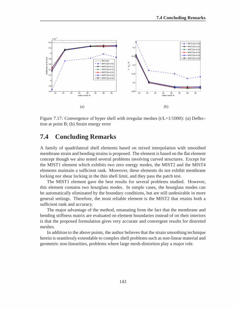
7.4 Concluding Remarks
10 15 20 25 30 35 40 454.6
4.8
5
5.2
5.4
5.6
5.8
6
6.2
6.4
x 10−3
Index mesh N
Def
lect
ion
at B
(cm
)
Ref solu.
MITC4(s=0.5)
MIST2(s=0.1)
MIST2(s=0.2)
MIST2(s=0.3)
MIST2(s=0.4)
MIST2(s=0.5)
(a)
10 15 20 25 30 35 40 450.05
0.1
0.15
0.2
0.25
0.3
Index mesh N
1 −
Eh /
E
MITC4(s=0.5)
MIST2(s=0.1)
MIST2(s=0.2)
MIST2(s=0.3)
MIST2(s=0.4)
MIST2(s=0.5)
(b)
Figure 7.17: Convergence of hyper shell with irregular meshes (t/L=1/1000): (a) Deflec-tion at point B; (b) Strain energy error
7.4 Concluding Remarks
A family of quadrilateral shell elements based on mixed interpolation with smoothedmembrane strain and bending strains is proposed. The element is based on the flat elementconcept though we also tested several problems involving curved structures. Except forthe MIST1 element which exhibits two zero energy modes, the MIST2 and the MIST4elements maintain a sufficient rank. Moreover, these elements do not exhibit membranelocking nor shear locking in the thin shell limit, and they pass the patch test.
The MIST1 element gave the best results for several problemsstudied. However,this element contains two hourglass modes. In simple cases,the hourglass modes canbe automatically eliminated by the boundary conditions, but are still undesirable in moregeneral settings. Therefore, the most reliable element is the MIST2 that retains both asufficient rank and accuracy.
The major advantage of the method, emanating from the fact that the membrane andbending stiffness matrix are evaluated on element boundaries instead of on their interiorsis that the proposed formulation gives very accurate and convergent results for distortedmeshes.
In addition to the above points, the author believes that thestrain smoothing techniqueherein is seamlessly extendable to complex shell problems such as non-linear material andgeometric non-linearities, problems where large mesh-distortion play a major role.
143

Chapter 8
A node-based smoothed finite elementmethod: an alternative mixed approach
8.1 Introduction
It is known that a stabilized conforming nodal integration technique has been applied byChenet al. (2001) for stabilizing the solutions in the context of meshfree methods andlater applied in the natural-element method (Yoo et al. (2004); Yvonnetet al. (2004);Cescotto & Li(2007)). Liu et al have applied this technique to formulate the linear con-forming point interpolation method (LC-PIM) (Liu et al. (2006b); Zhanget al. (2007)),the linearly conforming radial point interpolation method(LC-RPIM) (Liu et al.(2006a)),and the element-based smoothed finite element method (elemental SFEM) (Liu et al.(2007a)). ThenLiu & Zhang (2007) have explained intuitively and showed numericallythat the LC-PIM yields an upper bound in the strain energy when a reasonably fine meshis employed. Recently,Liu et al. (2007c) proposed a node-based smoothed finite ele-ment method (N-SFEM) for solid mechanics problems. In the N-SFEM, the domain dis-cretization is still based on elements but the calculation of the system stiffness matrix isperformed on cells each of which is associated with a single node, and the strain smooth-ing technique (Chenet al. (2001)) is used. The numerical results demonstrated that theN-SFEM possesses the following properties: 1) it gives an upper bound (in the case ofhomogeneous essential boundary conditions) in the strain energy of the exact solutionwhen meshes are sufficiently fine; 2) it is relatively immune from volumetric locking; 3)it allows the use of polygonal elements with an arbitrary number of sides; 4) no mappingor coordinate transformation is involved in the N-SFEM and its element is allowed to beof arbitrary shape. The problem domain can be discretized inmore flexible ways, andeven severely distorted elements can be used. All these features have been demonstratedin detail inLiu et al. (2007c) using many numerical examples and elements of complexshapes including polygon with an arbitrary number of sides,extremely distorted quadri-lateral elements. However, the related theory has not been set up fully to provide moregeneral theoretical explanation for the N-SFEM.
144

8.2 The N-SFEM based on four-node quadrilateral elements (NSQ4)
The aim of this chapter is to elucidate the properties of the N-SFEM and establish thenodal strain smoothing based on the Hellinger-Reissner principle, and formulate a four -node quadrilateral element node quadrilateral element in the setting of N-SFEM termed asNSQ4(Liu et al. (2007c)). In the present N-SFEM with NSQ4 elements, the domain dis-cretization is the same as that of the standard FEM and the bilinear interpolation functionsof the original displacement FEM model are still used. A quasi-equilibrium quadrilateralelement based on the following properties of the NSQ4 is obtained: 1) As long as theexternal forces are non-zero, strain energy is an upper bound of the exact solution whenthe used mesh is reasonably fine; 2) volumetric locking is eliminated naturally. Moreoverthe accuracy and convergence of the present N-SFEM will be proved by a rigorous math-ematical proofs on which affirms the reliability of present method theoretically. Finally,all these theories will be confirmed numerically.
8.2 The N-SFEM based on four-node quadrilateral ele-ments (NSQ4)
Assumed that the problem domainΩ is divided into smoothing cells (Liu et al. (2007c))associated with nodes such thatΩ = Ω(1)∪Ω(2) ∪ ....∪Ω(Nn) and Ω(i)∩Ω(j) = ∅, i 6= jin whichNn is the total number of field nodes located in the entire problem domain. Forfour-node quadrilateral elements, the cellΩ(k) associated with the nodek is created byconnecting sequentially the mid-edge-point to the intersection of two bi-medians of thesurrounding four-node quadrilateral elements as shown in Figure 8.1. As a result, eachfour-node quadrilateral element will be subdivided into four sub-domains and each sub-domain is attached with the nearest field node, e.g.Liu et al. (2007c). The cellΩ(k)
associated with the nodek is then created by combination of each nearest sub-domain ofall elements around the node k,Ω(k) = Ω
(k)1 ∪ Ω
(k)2 ∪ Ω
(k)2 ∪ Ω
(k)4 . The areasA(k) of the
nodal smoothing cells are computed by
A(k) =∑
c∈T (k)
Ac (8.1)
whereT (k) is the set of subcellsc associated with nodek andAc is the area of the subcells.Introducing now the node-based strain smoothing operation,
εkij(u
h) =1
A(k)
∑
c∈T (k)
Acεcij(u
h) (8.2)
where
εcij(u
h) =1
Ac
∫
Ω(k)c
εij(x)dΩ =1
2Ac
∫
∂Ω(k)c
(uhi nj + uh
j ni)dΓ (8.3)
andAc =∫Ω
(k)c
dΩ is the area of the subcellΩ(k)c .
145

8.2 The N-SFEM based on four-node quadrilateral elements (NSQ4)
Figure 8.1: Example of the node associated with subcells: The symbols (•), () and ()denote the nodal field, the mid-edge point and the intersection point of two bi-medians ofQ4 element, respectively
Inserting Equation (8.3) to Equation (8.2) and rearranging in the reduced form, one ob-tains the smoothed strain field (Liu et al. (2007c)) defined as
εkij(u
h) =1
A(k)
∫
Γ(k)
(niuj + njui)dΓ (8.4)
Substituting Equation (2.18) into Equation (8.4), the smoothed strain at the nodek can beformulated by the following matrix form based on nodal displacements
εk =∑
I∈N(k)
BI(xk)qI ≡ Bq (8.5)
whereN (k) is the number of nodes that are directly connected to nodek andBI(xk) istermed as the smoothed strain gradient matrix on the cellΩ(k) and is calculated numeri-cally by
BI(xk) =1
A(k)
∫
Γ(k)
NIn(k)(x)dΓ (8.6)
When a linear compatible displacement field along the boundary Γ(k) is used, one Gaus-sian point is sufficient for line integration along each segment of boundaryΓ(k)
b of Ω(k),Equation (8.6) can be expressed as
BI(xk) =1
A(k)
nb∑
b=1
NI(xGb )n(k)(xG
b )l(k)b (8.7)
wherenb is the total number of edges ofΓ(k), xGb is the midpoint (Gaussian point) of the
boundary segment ofΓ(k)b , whose length and outward unit normal matrix are denoted as
146

8.3 A quasi-equilibrium element via the 4-node N-SFEM element
l(k)b andn(k)(xG
b ), respectively. The stiffness matrixK of the system is then assembled bya similar process as in the FEM
K =Nn∑
k=1
K(k) (8.8)
whereK(k) is the stiffness matrix associated with nodek and is calculated by
K(k) =
∫
Ω(k)
BTDBdΩ = BTDBA(k) =1
A(k)
(∫
Γ(k)
n(k)NdΓ
)T
D
(∫
Γ(k)
n(k)NdΓ
)
(8.9)Equation (8.9) implies that in the NSQ4, the shape function itself is used to evaluate thestiffness matrix and no derivative of the shape function is needed. Because of using thebilinear shape functions for four-node quadrilateral elements, the displacement field alongthe boundariesΓ(k)
b of the domainΩ(k) is linear and compatible. Hence one Gauss pointis sufficient to compute exactly the integrations of Equation (8.6). The purpose of thissection is to recall briefly theoretical basis of the N-SFEM.More details can be found inLiu et al. (2007c).
8.3 A quasi-equilibrium element via the 4-node N-SFEMelement
The purpose of this section is to show some common propertiesof the NSQ4 and thepure equilibrium quadrilateral element (EQ4) given in Appendix A, and to establish avariational form derived from the Hellinger-Reissner principle.
8.3.1 Stress equilibrium inside the element and traction equilibriumon the edge of element
Without loss of generality, we assume that the problem domain is first divided into fourquadrilateral elements as shown in Figure8.2. it is then re-partitioned into the cellsΩ(k)
associated with nodes,k = 1, ..., 9 such thatΩ(i) ∩ Ω(j) = ∅, i 6= j. Let σ(k)e be the stress
vector of sub-domain in the element “e” belonging to the cellΩ(k). Assume that the finiteelement solutions of problem have already obtained. The stress vector at a nodek can becomputed through the smoothed strain at the nodek as
σ(k) = Dεk (8.10)
Based on Equation (8.2), the stressσ(k) in Equation (8.10) is termed as the smoothedstress on the cellΩ(k) . Hence, the stresses in all the sub-domains from adjacent elementsin the cellΩ(k) have the same values,
σ(k)e1
= σ(k)e2
= σ(k) (8.11)
147

8.3 A quasi-equilibrium element via the 4-node N-SFEM element
Figure 8.2: Stresses of background four-node quadrilateral cells and of the element:Thesymbols (•), () and () denote the nodal field, the mid-edge point and the intersectionpoint of two bi-medians of Q4 element, respectively
For details, we illustrate the contribution of the stress asshown in Figure8.2.
For node1 : σ(1)1 = σ(1)
2 : σ(2)1 = σ
(2)2 = σ(2)
3 : σ(3)2 = σ(3)
4 : σ(4)1 = σ
(4)3 = σ(4)
5 : σ(5)1 = σ
(5)2 = σ
(5)3 = σ
(5)4 = σ(5)
6 : σ(6)2 = σ
(6)4 = σ(6)
etc...
(8.12)
For elemente connected with four nodes;k1, k2, k3, k4, the “element” stress can be re-constructed by averaging the nodal stresses:
σe =σ
(k1)e + σ
(k2)e + σ
(k3)e + σ
(k4)e
4(8.13)
The traction on edgeij connecting nodei andj of element “e” can be constructed by
teij = nij
(σ(i)
e + σ(j)e
)/2 (8.14)
wherenij is the matrix of outward normals on edgeij. By the above construction, equili-brating tractions on the common side of adjacent elements are always ensured. It is clearthat in the present NSQ4, the equilibrium is satisfied strongly inside the element and onboundary of the element. However, the tractions along interfaces of the cell are not inequilibrium, and exists a stress gap. Based on numerical experiences below, the NSQ4model can be considered as a quasi-equilibrium model that does not seek equilibrium forevery point in the whole domain, but constitutes equilibrium status only in node-based
148

8.3 A quasi-equilibrium element via the 4-node N-SFEM element
smoothing domains resulting in a sufficient softening in thediscretized model. As a re-sult, it can provide an upper bound to the exact solution in the energy norm for elasticityproblems.
8.3.2 The variational form of the NSQ4
We start with the Hellinger–Reissner variational principle, e.g.Pian & Wu(2006), wherethe arbitrary stressσ and the displacementu are considered as independent field variables.Two 2-field variational principles result:
ΠHR(σ,u) =
∫
Ω
(−1
2σijD
−1ijklσkl + σij
1
2(ui,j + uj,i)− biui
)dΩ−
∫
Γt
tiuidΓ (8.15)
Equation (8.15) can be expressed through the smoothing cells as follows
ΠHR =
Nn∑
k=1
(∫
Ω(k)
[−1
2σijD
−1ijklσkl + σij
1
2(ui,j + uj,i)− biui]dΩ−
∫
Γ(k)t
tiuidΓ
)
(8.16)whereΓ(k) is the entire boundary of the cell andΓ
(k)t is the portion of the element boundary
over which the prescribed surface tractionst are applied.An integration part of the second term in the right hand side of Equation (8.16) be-
comes∫
Ω(k)
σij1
2(ui,j + uj,i)dΩ =
∫
Γ(k)
σij1
2(niuj + njui)dΓ−
∫
Ω(k)
uiσij,jdΩ (8.17)
Assuming that a constant stressσ is chosen, and inserting Equation (8.17) back Equa-tion (8.16), one hasΠHR =
Nn∑
k=1
(−1
2σijD
−1ijklσklA
(k) + σij1
2
∫
Γ(k)
(niuj + njui)dΓ−∫
Ω(k)
biuidΩ−∫
Γ(k)t
tiuidΓ
)
(8.18)In this principle, the variation of stress field leads to
D−1ijklσklA
(k) =1
2
∫
Γ(k)
(niuj + njui)dΓ (8.19)
This implies that there exists the strain fieldεij = D−1ijklσkl such that
εij =1
2A(k)
∫
Γ(k)
(niuj + njui)dΓ (8.20)
This shows that the smoothed strain in Equation (8.4) that used in the N-SFEM can de-rived from the Hellinger-Reissner variational justification. Therefore, we obtain the vari-ational principles of two fields based on the smoothed strainε and the displacementu as
149

8.4 Accuracy of the present method
ΠHR(ε,u) =1
2
Nn∑
k=1
(εijDijklεijA
(k) −∫
Ω(k)
biuidΩ−∫
Γ(k)t
tiuidΓ
)(8.21)
which is identical to the often used mixed approach. This means that the NSQ4 has afoundation on the Hellinger-Reissner variational principle.
8.4 Accuracy of the present method
Here it will be shown in energy form that the work of the present N-SFEM is larger thanthat of the displacement approach. Or in other words, the stiffness matrix of the NSQ4element is softer than that of the Q4 element and therefore the present model is moreaccurate than the displacement model.
8.4.1 Exact and finite element formulations
Based on the Hellinger-Reissner variational principle, the weak form is to find the solution(σ,u) such that the functional
ΠHR(σ,u) = (σ, ∂u)− 1
2(σ,D−1σ)− f(u) (8.22)
is maximum for all stress fieldsσ ∈ S and minimum for all displacement fieldsu ∈ V.Hence we have the following weak statement
(τ , ∂u) = (τ ,D−1σ), ∀τ ∈ S
(σ, ∂v) = f(v), ∀v ∈ V0(8.23)
LetVh ⊂ V andSh ⊂ S be a finite element space. The weak form for the approximatedsolution becomes: Find(σh,uh) ∈ Sh × Vh such that
(τ , ∂uh) = (τ ,D−1σh), ∀τ ∈ Sh
(σh, ∂vh) = f(vh), ∀vh ∈ Vh0
(8.24)
Equation (8.24)1 means thatD−1σh is a result of the projection of the element∂uh of S
into Sh. Therefore there exists ae projection operatorPh from S to Sh such that
D−1σh = Ph∂uh or σh = DPh∂uh (8.25)
UsingPh, we have(σh, ∂vh) = (σh, Ph∂vh) (8.26)
Using Equations (8.25) and (8.26), Equation (8.24)2 becomes
(DPh∂uh, Ph∂v) = f(v), ∀v ∈ Vh0 (8.27)
which is a displacement-like formulation. WhenPh is an identity operator, the conven-tional displacement approach is recovered.
150

8.5 Convergence of the present method
8.4.2 Comparison with the classical displacement approach
For simplicity, we assumeVh = Vh0 . Let wh be the solution of the classical displacement
model. It verifies(D∂wh, ∂vh) = f(vh), ∀vh ∈ V
h (8.28)
Settingwh = vh and using the definition of energy norm in Chapter 2, one sets
∥∥wh∥∥2
E= f(wh) (8.29)
Thereby, from (8.27), we reach the following inequalityf(wh) = (DPh∂uh, Ph∂wh) = (DPh∂uh, ∂wh) =
(Ph∂uh, ∂wh
)E
≤∥∥Ph∂uh
∥∥E
∥∥∂wh∥∥
E=√
f(uh)√
f(wh)⇔ f(wh) ≤ f(uh) (8.30)
This proves that the work of the solution of the presented approach (the mixed approach)is always greater than that of the solution of the classical displacement approach.
8.5 Convergence of the present method
The objective of this section is to establish a priori error estimation which ensures theconvergence of proposed approach.
8.5.1 Exact and approximate formulations
Let a(σ, τ ) = (D−1σ, τ ) be the bilinear form and the norm inL2 is denoted by‖·‖. Theexact formulation is to findσ ∈ S andu ∈ V such that
a(σ, τ ) = (τ , ∂u), ∀τ ∈ S
(σ, ∂v) = f(v), ∀v ∈ V0(8.31)
Hence the following properties of the bilinear forma(.; .) are satisfied:
∃α > 0 : a(σ, σ) ≥ α ‖σ‖2 , ∀σ ∈ S
∃M > 0 : a(σ, τ ) ≤M ‖σ‖ ‖τ‖ , ∀τ ∈ S(8.32)
and on continuity condition, one has
(σ, ∂v) ≤ ‖σ‖ ‖∂v‖ (8.33)
Moreover, Brezzi’s condition is fulfilled as
supσ∈S
(σ, ∂u)
‖σ‖ ≥ (∂u, ∂u)
‖∂u‖ = ‖∂u‖ , (constantβ = 1) (8.34)
So, there exists a unique solution to the problem.
151

8.5 Convergence of the present method
Let us now define theZ-space asZ = σ ∈ S | ∀v ∈ V, (σ, ∂v) = 0 and Z(f) =σ ∈ S | ∀v ∈ V, (σ, ∂v) = f(v). The approximate spaces forZ andZ(f) are denotedasZh = σh ∈ S
h | ∀vh ∈ Vh, (σh, ∂vh) = 0 and Zh(f) = σh ∈ S
h | ∀vh ∈Vh, (σh, ∂vh) = f(vh). Again for simplicity, it is assumed thatVh = Vh
0
The finite element solution for the problem is to find(σh,uh) ∈ Sh × Vh such that
a(σh, τ h) = (τ h, ∂uh), ∀τ h ∈ Sh
(σh, ∂vh) = f(vh), ∀vh ∈ Vh (8.35)
Assume that the present element is stable and convergent, hence there exists a constantβh > 0 such that
supσh∈Sh
(σh, ∂uh)
‖σh‖ ≥ βh
∥∥∂uh∥∥ (8.36)
The condition (8.36) plays a fundamental role in the convergence analysis of mixed finiteelement methods, e.g.Brezzi & Fortin(1991).
8.5.2 A priori error on the stress
Let σh be the approximated solution andτ h be another element ofZh(f), i.e,σh− τ h ∈Zh. One has
a(σh − τ h, σ − σh) = (σh − τ h, ∂u)− (σh − τ h, ∂uh) = (σh − τ h, ∂u) + 0= (σh − τ h, ∂u− ∂vh) ≤
∥∥σh − τ h∥∥∥∥∂u− ∂vh
∥∥ , ∀vh ∈ Vh
(8.37)and of course
a(σh − τ h, σ − τ h) ≤M∥∥σh − τ h
∥∥∥∥σ − τ h∥∥ (8.38)
From Equations (8.32),(8.37)-(8.38), it results that
α∥∥σh − τ h
∥∥2 ≤ a(σh − τ h, σh − τ h)≤∥∥σh − τ h
∥∥∥∥∂u− ∂vh∥∥+ M
∥∥σh − τ h∥∥∥∥σ − τ h
∥∥ (8.39)
Hence ∥∥σh − τ h∥∥ ≤ 1
α
∥∥∂u− ∂vh∥∥+
M
α
∥∥σ − τ h∥∥ (8.40)
Now,
∥∥σ − σh∥∥ ≤
∥∥σ − τ h∥∥+
∥∥σh − τ h∥∥ ≤ 1
α
∥∥∂u− ∂vh∥∥+ (1 +
M
α)∥∥σ − τ h
∥∥(8.41)
and as it is true for anyvh ∈ Vh and for anyτ h ∈ Zh(f), one obtains
∥∥σ − σh∥∥ ≤ 1
αinf
vh∈Vh
∥∥∂u− ∂vh∥∥+ (1 +
M
α) infτ h∈Zh(f)
∥∥σ − τ h∥∥ (8.42)
152

8.5 Convergence of the present method
It is noted that the last term is embarrassing as the infinum has to be taken on a sub-space ofSh. However, considering a stress fieldςh ∈ Sh, one knows that there exits aθh ∈ Zh
⊥such that
(θh, ∂vh) = (σ − ςh, ∂vh) = f(vh)− (ςh, ∂vh), ∀vh ∈ Vh (8.43)
Now we have
∥∥θh∥∥ ≤ 1
βhsup
vh∈Vh
(θh, ∂vh)
‖∂vh‖ ≤ 1
βhsup
vh∈Vh
∥∥σ − ςh∥∥∥∥∂vh
∥∥‖∂vh‖ =
1
βh
∥∥σ − ςh∥∥ (8.44)
By choosingχh = θh+ςh ⇒ χh ∈ Zh(f) as(θh+ςh, ∂vh) = (σ, ∂vh) = f(vh), ∀vh ∈Vh and noting
∥∥σ − χh∥∥ ≤
∥∥σ − ςh∥∥+
∥∥θh∥∥ = (1 +
1
βh
)∥∥σ − ςh
∥∥ , the following es-
timation is achieved:
∥∥σ − χh∥∥ ≤ (1 +
1
βh
) infςh∈Sh
∥∥σ − ςh∥∥ (8.45)
And therefore one obtains
infτ h∈Zh(f)
∥∥σ − τ h∥∥ ≤ (1 +
1
βh) infςh∈Sh
∥∥σ − ςh∥∥ (8.46)
Finally, assembling (8.46) to (8.42), a priori error on the stress is obtained as
∥∥σ − σh∥∥ ≤ 1
αinf
vh∈Vh
∥∥∂u− ∂vh∥∥+ (1 +
M
α)(1 +
1
βh) infςh∈Sh
∥∥σ − ςh∥∥ (8.47)
Note that in pure displacement model the first term of (8.47) is present and in pure equi-librium model the second term is present. The convergence will disappear ifβh = O(h)and
∥∥σ − ςh∥∥ ≤ Ch. That is the well-known drawback of mixed approaches.
8.5.3 A priori error on the displacement
Let uh be the approximate solution and another valuevh ∈ Vh. It satisfies
∥∥∂uh − ∂vh∥∥ ≤ 1
βhsup
τ h∈Sh
(τ h, ∂uh − ∂vh)
‖τ h‖ (8.48)
and(τ h, ∂uh − ∂vh) = (τ h, ∂uh − ∂u) + (τ h, ∂u− ∂vh)= a(τ h, σ − σh) + (τ h, ∂u− ∂vh)≤M
∥∥τ h∥∥∥∥σ − σh
∥∥+∥∥τ h
∥∥∥∥∂u− ∂vh∥∥
(8.49)
Hence ∥∥∂uh − ∂vh∥∥ ≤ M
βh
∥∥σ − σh∥∥+
1
βh
∥∥∂u− ∂vh∥∥ (8.50)
153

8.6 Numerical tests
By the triangle inequality
∥∥∂u− ∂uh∥∥ ≤
∥∥∂u− ∂vh∥∥+∥∥∂uh − ∂vh
∥∥ ≤ M
βh
∥∥σ − σh∥∥+(1+
1
βh)∥∥∂u− ∂vh
∥∥
(8.51)for anyvh ∈ Vh, a priori error on the displacement is accomplished as
∥∥∂u− ∂uh∥∥ ≤ M
βh
∥∥σ − σh∥∥+ (1 +
1
βh) inf
vh∈Vh
∥∥∂u− ∂vh∥∥ (8.52)
in which∥∥σ − σh
∥∥ derived from Equation (8.47). It is clear that∥∥∂u− ∂uh
∥∥ contains
a factor1
β2h
. So a “bad”βh will cause that the displacements are worse than the stresses.
Thus the formulations on a priori error on the stress and displacement fields wereestablished. The convergence of the presented method is ensured and conducted by thesatisfaction Brezzi’s condition.
8.6 Numerical tests
As discussed in Section8.3 and Section8.4, the NSQ4 possesses advantage character-istics of pure equilibrium element and mixed element; 1) theequilibrium stresses insideand the continuity of stress resultants across interface ofthe element are ensured stronglybut may not be satisfy along interfaces of cell, and 2) its connectors are still at the cor-ner nodes as the displacement model used. Therefore, the NSQ4 element is consideredas the incorporation of pure equilibrium approach and mixedmodel, and is proposed tobe a quasi-equilibrium approach. All theoretical proofs will be confirmed with numer-ically following tests again. In order to make comparison with the NSQ4 element, theformulations of the pure equilibrium quadrilateral element (EQ4) are given in AppendixA.
8.6.1 Cantilever loaded at the end
A cantilever with lengthL = 8 and heightD = 4 is studied as a benchmark here, whichis subjected to a parabolic traction at the free end as shown in Chapter 3. The cantileveris assumed to have a unit thickness so that plane stress condition is valid. The analyticalsolution is available and can be found in a textbook byTimoshenko & Goodier(1987).
The related parameters are taken as in Chapter 3. In the computations, the nodes on theleft boundary are constrained using the exact displacements obtained fromTimoshenko& Goodier (1987) and the loading on the right boundary is a distributed parabolic shearstress.
To assess the convergence rate, the same asPuso & Solberg(2006), the error in energy
154

8.6 Numerical tests
norm for node-based smoothed finite elements is defined by
∥∥u− uh∥∥
E=
(Nn∑
k=1
(ε(xk)− εk(xk)
): D :
(ε(xk)− εk(xk)
)A(k)
)1/2
(8.53)
Figure 8.3: Uniform mesh with 512 quadrilateral elements for the cantilever beam
The domain discretization for uniform meshes of quadrilateral elements is shown inFigure8.3. Herein, the connectors of the Q4 and NSQ4 elements are established at thecorner nodes of quadrilateral element while those of the (EQ4) element are at the middlepoints along the element edges.
Figure8.4depicts graphically the strain energy obtained against number of elementsand, also, the rate of convergence. It can be seen that the NSQ4 overestimates the strainenergy compared to the pure equilibrium element (EQ4) whilethe Q4 underestimatesthe strain energy. Moreover, in this problem, the NSQ4 element is more accurate thanEQ4 element with coarse mesh. As resulted in the error of energy norm, solutions of
0 100 200 300 400 500
0.034
0.036
0.038
0.04
0.042
0.044
0.046
0.048
0.05
0.052
0.054
Number of elements
Str
ain
ener
gy
ExactQ4EQ4NSQ4
(a)
−1.2 −1.1 −1 −0.9 −0.8 −0.7 −0.6 −0.5 −0.4 −0.3
−3.5
−3
−2.5
−2
−1.5
−1
log10
(h)
log 10
(Err
or in
ene
rgy
norm
)
Q4EQ4NSQ4
0.997
1.486
2.003
(b)
Figure 8.4: The convergence of cantilever: (a) Strain energy ; (b) The convergence rate
155

8.6 Numerical tests
the SNQ4 are more accurate and achieve a higher convergence rate than FEM-Q4. It isknown that if the conforming model(Q4) is exploited, the convergence rate in energy normshould be mathematically equal to 1.0, and if a pure equilibrium model (EQ4) is used, theconvergence rate in energy norm should equal mathematically 2.0, see e.g.Johnson &Mercier (1979). It is clear that the equilibrium model gains the superconvergence ratein the energy norm which was demonstrated theoretically. For the NSQ4, the rate ofconvergence in energy norm shown in Figure8.4b is 1.486 and is higher than that of theQ4. As discussed in previous sections of this chapter, the equilibrium for the SNQ4 isensured strongly in the elements and inside the smoothing cells while on all the interfacesof the smoothing cells equilibrating tractions may not be ensured and only the continuityof displacements is satisfied. Therefore, the rate of convergence in energy norm for manyproblems may be, theoretically, between 1.0 and 2.0, also see e.g.Liu & Zhang (2007).And in several cases the rate of convergence may be larger than 2.0. Thus the optimalvalue will depend on another forms of structure.
8.6.2 A cylindrical pipe subjected to an inner pressure
Figure8.5shows a thick cylindrical pipe, with internal radiusa = 0.1m, external radiusb = 0.2m, subjected to an internal pressurep = 6kN/m2. Because of the symmet-ric characteristic of the problem, we only calculate one quarter of cylinder as shown inFigure8.5. The discretization of the domain uses 4-node quadrilateral elements. Planestrain condition is considered and Young’s modulusE = 21000kN/m2 , Poisson’s ra-tio ν = 0.3. Symmetric conditions are imposed on the left and bottom edges, and outerboundary is traction free. The exact solution is given inTimoshenko & Goodier(1987).Again, Figure8.6a shows that the NSQ4 maintains the upper bound property of the strainenergy. However, the EQ4 element is more accurate than the NSQ4 element. The EQ4element exhibits a superconvergence in the energy norm while the NSQ4 provides the rateof convergence between 1.0 and 2.0 (as depicted by Figure8.6b).
8.6.3 Infinite plate with a circular hole
Figure8.7 represents a plate with a central circular hole of radiusa = 1m, subjectedto a unidirectional tensile load ofσ = 1.0N/m at infinity in the x-direction. Due to itssymmetry, only the upper right quadrant of the plate is modeled. Plane strain conditionis considered andE = 1.0 × 10³N/m2, ν = 0.3. Symmetric conditions are imposed onthe left and bottom edges, and the inner boundary of the hole is traction free. The exactsolution for the stress is (Timoshenko & Goodier(1987))
σ11(r, θ) = 1− a2
r2
[32cos 2θ + cos 4θ
]+ 3a4
2r4 cos 4θ
σ22(r, θ) = −a2
r2
[12cos 2θ − cos 4θ
]− 3a4
2r4 cos 4θ
τ12(r, θ) = −a2
r2
[12sin 2θ + sin 4θ
]+ 3a4
2r4 sin 4θ
(8.54)
where(r, θ) are the polar coordinates andθ is measured counterclockwise from the pos-itive x-axis. Traction boundary conditions are imposed on the right (x = 5.0) and top
156

8.6 Numerical tests
(a)
0 0.05 0.1 0.15 0.20
0.02
0.04
0.06
0.08
0.1
0.12
0.14
0.16
0.18
0.2
5
6
7
8
9
10
11
12
(b)
Figure 8.5: (a) A thick cylindrical pipe subjected to an inner pressure and its quartermodel; (b) A sample discretization of 1024 quadrilateral elements and distribution of vonMises stresses
157

8.6 Numerical tests
0 50 100 150 200 250 300 350 400 450 5002.5
2.55
2.6
2.65
2.7
2.75
2.8
2.85
2.9
Number of elements
Str
ain
ener
gy x
10−
5
ExactQ4EQ4NSQ4
(a)
−2 −1.9 −1.8 −1.7 −1.6 −1.5 −1.4 −1.3 −1.2 −1.1
−6
−5.5
−5
−4.5
−4
−3.5
log10
(h)
log 10
(Err
or in
ene
rgy
norm
)
Q4EQ4NSQ4
2.026
1.548
1.03
(b)
Figure 8.6: The convergence in energy of the cylindrical pipe: (a) Strain energy ; (b) Theconvergence rate
(y = 5.0) edges based on the exact solution Equation (8.54). The displacement compo-nents corresponding to the stresses are
u1(r, θ) = a8µ
[ra(κ + 1) cos θ + 2a
r((1 + κ) cos θ + cos 3θ)− 2a3
r3 cos 3θ]
u2(r, θ) = a8µ
[ra(κ− 1) sin θ + 2a
r((1− κ) sin θ + sin 3θ)− 2a3
r3 sin 3θ] (8.55)
whereµ = E/ (2 (1 + ν)), κ is defined in terms of Poisson’s ratio byκ = 3−4ν for planestrain cases. Figure8.7gives the discretization of the domain using 4-node quadrilateralelements. Figure8.8a shows the upper bound property of the strain energy of the NSQ4with fine enough meshes, while the Q4 give the lower bound of strain energy. As plottedin Figure8.8b, the superconvergent results in energy norm are obtained for the EQ4 andNSQ4 elements.For nearly incompressible case(ν = 0.4999999), Figure8.9plots the computed stressesobtained by the EQ4 element and the NSQ4 element. It is shown that both these elementsare in good agreement with the analytical solutions. Figure8.10depicts the behaviour oferror in the energy norm as Poissons ratio tends to 0.5. It is observed that insensitivity tolocking is evident for both EQ4 and NSQ4 whereas the FEM-Q4 isobviously subjectedto volumetric locking. Therefore the NSQ4 element possesses the advantage of beingrelatively immune from volumetric locking as the pure equilibrium element (EQ4).
8.6.4 Cook’s membrane
The benchmark problem studied in Chapter 3 and this model is recalled in Figure8.11.Under plane stress conditions, the reference value of the vertical displacement at the cen-
158

8.6 Numerical tests
(a)
0 1 2 3 4 50
0.5
1
1.5
2
2.5
3
3.5
4
4.5
5
0.5
1
1.5
2
2.5
(b)
Figure 8.7: (a) Infinite plate with a circular hole subjectedto uniform tensile loadσ0;(b) A sample discretization of 1024 quadrilateral elementsand distribution of von Misesstresses
0 500 1000 1500 2000 2500 3000 3500 4000
0.0118
0.0118
0.0118
0.0118
0.0118
0.0118
0.0119
Number of elements
Str
ain
ener
gy
EQ4NSQ4Q4Exact sol.
(a)
−2 −1.8 −1.6 −1.4 −1.2 −1−5
−4.5
−4
−3.5
−3
−2.5
−2
h
log 10
(Err
or in
ene
rgy
norm
)
Q4EQ4NSQ4
1.078
2.304
2.362
(b)
Figure 8.8: The convergence of the infinite plate a circular hole problem: (a) Strain energy; (b) The convergence rate
159

8.6 Numerical tests
1 1.5 2 2.5 3 3.5 4 4.5 51
1.2
1.4
1.6
1.8
2
2.2
2.4
2.6
2.8
3
Radial distance r
Str
ess
σ 11
Exact sol.EQ4NSQ4
(a)
1 1.5 2 2.5 3 3.5 4 4.5 50
0.05
0.1
0.15
0.2
0.25
0.3
0.35
0.4
Radial distance r
Str
ess
σ 22
Exact sol.EQ4NSQ4
(b)
Figure 8.9: Stresses of hole plate for incompressibility
0.4 0.49 0.499 0.4999 0.49999 0.499999 0.49999990
5
10
15
20
25
Possion’s ratio ν
Rel
ativ
e er
ror
in e
nerg
y no
rm(%
)
Q4EQ4NSQ4
Figure 8.10: Relative error in energy norm of hole plate using 256 elements with differentPoissons ratios
160

8.6 Numerical tests
ter of the tip section (C) inFredriksson & Ottosen(2004) is 23.9642 and the referencevalue of the strain energy given byMijuca & Berkovic (1998) is 12.015.
Here, the SNQ4 is compared with other elements listed in Table 8.1: Allman’s mem-brane triangle (AT) (Allman (1984)), assumed stress hybrid methods such as P-S element(Pian & Sumihara(1984)), Xie-Zhou’s element (ECQ4/LQ6)(Xie & Zhou (2004)), Zhou-Nie’s element (CH(0-1)) (Zhou & Nie(2001)) and HQM/HQ4 element (Xie (2005)), finiteelement primal-mixed approach (FEMIXHB) introduced byMijuca & Berkovic (1998).It is found that the SNQ4 solution overestimates the best reference solution while theother hybrid stress elements converge to this exact solution from below.
In addition to the results shown in Table8.1, the values obtained for the energy esti-mation and the displacement at the tip are presented in Figure8.12. It can be seen that theproposed element provides an improved solution in strain energy compared to the equi-librium element (EQ4). However the rate of convergence in the strain energy for the EQ4and NSQ4 is lower than the Q4 for this case. When we estimate the convergence of dis-placement, the very good behavior of the NSQ4 element is obvious for compressible andnearly incompressible materials. Further, the present element is compared to the stabi-lization elements byBelytschko & Bachrach(1986) andBelytschko & Bindeman(1991)and is good agreement with these elements.
Table 8.1: Results of displacement tip (at C) and strain energy for Cook’s problem
NodeDisplacement tip Strain energy
2× 2 4× 4 8× 8 2× 2 4× 4 8× 8
AT 19.67(27)(∗) 22.41(75) 23.45(243) 9.84 11.22 11.75P-S 21.13(18) 23.02(50) 23.69(162) 10.50 11.51 11.85
CH(0-1) 23.01(18) 23.48(50) 23.81(162) 11.47 11.75 11.91ECQ4/LQ6 23.05(18) 23.48(50) 23.81(162) 11.48 11.75 11.91HMQ/HQ4 21.35(18) 23.04(50) 23.69(162) 10.61 11.52 11.85FEMIXHB 22.81(35) 23.52(135) 23.92(527) 11.27 11.79 11.97
NSQ4 24.69(18) 25.38(50) 24.51(162) 12.29 12.70 12.27Ref 23.9642 23.9642 23.9642 12.015 12.015 12.015
(*) Number of degrees of freedom denoted in parenthesis
8.6.5 Crack problem in linear elasticity
A crack problem with data of the structure is considered as inChapter 3. Only half ofdomain is modeled with uniform meshes with the same aspect ratio and a distribution ofvon Mises stress is illustrated by Figure8.13. Note that, the solution of the crack problemincludes the strong singularity (namely ar−1/2 in stress) at the crack tip. In the presentstudy, we only estimate the results based on the global strain energy of entire domain.Hence discontinuity fields such as displacements and stresses along crack path should befurther considered by incorporating the present method into the extended finite element
161

8.6 Numerical tests
(a)
(b)
Figure 8.11: Cook’s membrane and a distribution of von Misesstress using 1024 elements
162

8.6 Numerical tests
101
10
15
20
25
30
Number of elements per edge
Cen
tral
dis
plac
emen
t tip
RefQ4Qm6QnewQBIFBKFEQ4SNQ4
(a)
5 10 15 20 25 30
6
8
10
12
14
16
18
20
22
24
26
28
Number of elements per side
Top
cor
ner
vert
ical
dis
plac
emen
t v
Q4SRIASMDASQBIASOIASOI(1/2)EQ4SNQ4
(b)
5 10 15 20 25 30
6
8
10
12
14
16
Number of elements per edge
Str
ain
ener
gy
RefQ4EQ4NSQ4
(c)
−2 −1.8 −1.6 −1.4 −1.2 −1 −0.8
−0.8
−0.6
−0.4
−0.2
0
0.2
0.4
log10
(h)
log 10
(Err
or in
str
ain
ener
gy)
Q4 EQ4 NSQ4
0.9
0.76
0.82
(d)
Figure 8.12: Convergence in strain energy and the central displacement for the Cookmembrane: (a) Displacement at C (ν = 1/3), plane stress ; (b) Displacement at C (ν =0.4999), plane strain; and (c) Strain energy (ν = 1/3); (d) Convergence rate in strainenergy (ν = 1/3)
163

8.6 Numerical tests
method (XFEM) (Moeset al.(1999)) which has been recently proved to be advantageousto solve crack problems.
Figure 8.13: A distribution of von Mises stress for crack using the SNQ4 element
10 20 30 40 50 606000
7000
8000
9000
10000
11000
12000
Number of elements per edge
Str
ain
ener
gy
RefQ4EQ4NSQ4
(a)
−2.2 −2 −1.8 −1.6 −1.4 −1.21.1
1.2
1.3
1.4
1.5
1.6
1.7
log10
(h)
log 10
(Err
or in
str
ain
ener
gy)
Q4EQ4NSQ4
0.510
0.552
0.476
(b)
Figure 8.14: Convergence in energy for the crack problem:(a) Strain energy ; (b) Theconvergence rate
The convergence of strain energy for the NSQ4 and EQ4 elements is illustrated in Fig-ure 8.14. As a result, the upper bound property of the NSQ4 on the strain energy isobtained for meshes that are not too coarse. The NSQ4 elementprovides the better solu-tion in strain energy compared to the EQ4 element for this problem and does not convergemonotonically.
164

8.6 Numerical tests
8.6.6 The dam problem
A 2D dam under hydrostatic loads and its geometry data (Cugnon(2000) andNguyen(2006)) are shown in Figure8.15. Plane strain conditions are assumed and numericalparameters are: thickness = 1, hydrostatic load p = 103, Young’s modulusE = 2× 10¹²,Poisson’s ratioν = 0.3. An illustration of 972 quadrilateral elements and a distribution ofvon Mises stress shown in Figure8.16. We can realize a singularity in stress at the left andright corners of dam. Hence, an adaptive approach might be useful. Figure8.17a gives theenergy convergence of the Q4 and the NSQ4. Because an exact solution of this problem isnot available, an estimated solution may be obtained by meanof two extrapolated energyvalues; one is of the Q4 element and the other is the NSQ4 element. The estimated strainenergy is0.52733 × 10−4. The rate of convergence in strain energy is also exhibited byFigure8.17b. The good convergence of the NSQ4 is observed.
Figure 8.15: A 2D dam problem
8.6.7 Plate with holes
We consider a three-hole plate under plane strain conditions. This problem was investi-gated byPaulinoet al. (1999) for self-adaptive procedures. Numerical parameters are:thickness = 1, a uniform load p = 1.0, Young’s modulusE = 2 × 10⁵, Poisson’s ratioν = 0.3. The geometry and boundary conditions of problem are shown in Figure8.18.
Figure8.19 gives an illustration of quadrilateral element meshes and adistributionof von Mises stress. We can realize the regions of stress concentration as shown inFigure 8.19b. Figure8.20a plots the strain energy of the Q4 and the NSQ4. An ex-act solution of this problem is unknown and the extrapolatedenergy value is hence ex-ploited. The estimated strain energy is1.59196. Figure8.17b gives the rate of con-vergence in strain energy corresponding to dimensionless lengthh = 1/
√N , where
N = [316 762 2262 8774 19094] is the number of degrees of freedom (D.O.F) re-
165

8.6 Numerical tests
0 50 100 150 200 250 300
0
50
100
150
200
50
100
150
200
250
300
350
400
Figure 8.16: Example of 972 quadrilateral elements and a distribution of von Mises stress
0 10 20 30 40 50
4.5
5
5.5
6
6.5x 10
−5
Number of elements per edge
Str
ain
ener
gy
Estimated sol.Q4NSQ4
(a)
−2 −1.8 −1.6 −1.4 −1.2 −1−3.2
−3.1
−3
−2.9
−2.8
−2.7
−2.6
−2.5
−2.4
−2.3
log10
(h)
log 10
(Err
or in
str
ain
ener
gy)
Q4NSQ4
0.869
0.714
(b)
Figure 8.17: Convergence in energy for the dam problem:(a) Strain energy ; (b) Theconvergence rate
166

8.6 Numerical tests
Figure 8.18: A 2D plate with holes
0 50 100 150 200 250 300 350 400 4500
50
100
150
200
250
300
350
(a) (b)
Figure 8.19: Example of 1022 quadrilateral elements and a distribution of von Misesstress using the NSQ4
167

8.7 Concluding remarks
1 1.5 2 2.5 3 3.5 4 4.5 5
1.45
1.5
1.55
1.6
1.65
1.7
Index
Str
ain
ener
gyEstimated sol.Q4NSQ4
(a)
−2.2 −2 −1.8 −1.6 −1.4 −1.2
−1.2
−1.1
−1
−0.9
−0.8
−0.7
−0.6
−0.5
−0.4
−0.3
−0.2
log10
(h)
log 10
(Err
or in
str
ain
ener
gy)
Q4NSQ4
0.77
0.98
(b)
Figure 8.20: Convergence in energy for the plate with holes:(a) Strain energy ; (b) Theconvergence rate
maining after imposing boundary conditions. The NSQ4 converges monotonically fromabove and is more accurate than the Q4.
8.7 Concluding remarks
In this chapter, the NSQ4 is compared to a variety of four-node quadrilateral elementsfrom the literature. Based on formulations and numerical examples, the following con-clusions are remarked:
• The stress field is a statically admissible within the element (equilibrated insidethe element and transmitted continuously over adjacent elements). This property iswell-known in the equilibrium finite models. Additionally,the displacement fieldis continuous through element boundaries while the equilibrium models are de-fined by average displacements. When smoothing cells are used, the equilibriumof stresses is satisfied inside the cells but reciprocity between tractions across theirboundaries may not be ensured. In this context, the nodally strain smoothing isalso obtained from the justification of a mixed approach. Therefore, the NSQ4 canbe seen as a quasi - equilibrium approach of pure equilibriummodel. As a result,when homogeneous displacements are prescribed, the NSQ4 always achieves anoverestimation of the true energy when the mesh is sufficiently fine.
• The accuracy and convergence of the NSQ4 have been proved theoretically in theframework of functional analysis.
168

8.7 Concluding remarks
• For all examples tested, the NSQ4 is in good agreement with the analytical solution.The accuracy of the NSQ4 is also compared with other elements.
• In an analogous manner to that advocated for the EQ4, the NSQ4overcomes rela-tively volumetric locking.
• Moreover, in the NSQ4, field gradients are computed directlyonly using shapefunctions themselves and no derivative of shape function isneeded. The shape func-tions are created in a trivial, simple and explicit manner. Unlike the conventionalFEM using isoparametric elements, as no coordinate transformation or mapping isperformed in the NSQ4, no limitation is imposed on the shape of elements usedherein. Even severely distorted elements are allowed. Hence domain discretizationis more flexible than FEM.
• Last but not least, the NSQ4 is more convenient to compute directly the nodalstresses while the standard displacement models often use post-processing proce-dure to recover these stresses. Therefore, the NSQ4 is very promising to obtain asimple and practical procedure for the stress analysis of the FEM using four-nodedquadrilateral elements.
169

Chapter 9
Conclusions
The method exploited here originated from mesh-free research. The main aim of smooth-ing strain fields is to eliminate the instability of direct nodal integration techniques inthe mesh-free methods when the shape function derivatives at nodes vanish. The directnodal integration (NI) often causes large oscillations in the solution because it violatesintegration constraints (IC) that any meshless method needs to pass similarly to the patchtest as in FEM. Although the stabilized conforming nodal integration (SCNI) using thestrain smoothing method avoids instability of the NI and obtains good accuracy and highconvergence rates, the non-polynomial or usually complex approximation space increasesthe computational cost of numerical integration.
The objective of this thesis is therefore to present numerous applications of the strainsmoothing method to finite elements, namely SFEM, for analyzing static and dynamicstructures of two and three dimensional solids, plates, shells, etc. In finite elements,the strain smoothing technique is similar to stabilized conforming nodal integration formeshfree methods. Except some special cases of three-dimensional solids where stan-dard interior integration is used, the stiffness matrix is computed by boundary integrationinstead of the standard interior integration of the traditional FEM. This permits to utilizedistorted meshes. In all the numerical examples tested, it is observed that the presentmethod is more accurate than the standard FEM element for a lower computational cost.
This thesis has shown the following results:- Based on a Taylor series, the strain smoothing field is considered as an alterna-
tive form of the enhanced assumed strain method. The smoothed strains are sum of twoterms; one is the compatible strains and the other is the enhanced strains. A rigorousvariational framework based on the Hu – Washizu assumed strain variational form wasshown to be suitable. It is found that solutions yielded by the SFEM are in a spacebounded by the standard, finite element solution (infinite number of smoothing cells)and a quasi-equilibrium finite element solution (a single cell). The benchmark problemsof compressible and incompressible two and three dimensional elasticity have adequatelychosen and analyzed in detail. It is shown that the SFEM always achieves higher accuracyand convergence rates than the standard finite element method, especially in the presence
170

of incompressibility, singularities or distorted meshes,for a smaller computational cost.- New 8 noded hexahedral elements based on the smoothed finiteelement method
(SFEM) with various numbers of smoothing cells were proposed. It was observed thatlow numbers of smoothing cells lead to higher stress accuracy but instabilities; high num-bers yield lower stress accuracy but are always stable. Hence a stabilization procedureis formulated which is based on the linear combination of theone subcell element andthe four or eight subcell element. As a result, zero energy modes are suppressed and thestabilized elements are free of volumetric locking and obtain higher accuracy than theeight-node hexahedral brick element.
- A quadrilateral Mindlin - Reissner plate element with smoothed curvatures, the so-called MISCk element, was proposed. The curvature at each point is smoothed via aspatial averaging. The smoothed curvatures are also considered as the enhanced assumedcurvatures while the approximation of the shear strains follows the assumed natural strain(ANS) method. The reliability of the proposed element is confirmed through numericaltests. It is seen that the present method is robust, computationally inexpensive and simul-taneously very accurate and free of locking. The most promising feature of the presentelements is their insensitivity to mesh distortion.
- A further extension of the MISCk element combined with a stabilization technique,namely SMISCk element, to the free vibration analysis of Mindlin – Reissner plates wasinvestigated. It was also remarked that the present elements are free of shear locking forvery thin plates and give a good agreement with analytical solutions and published results.From frequency analysis, the MISCk elements exhibit higheraccuracy than the MITC4element for all examples tested. Moreover, if associated with the stabilization technique,the SMISCk elements are always superior in terms of convergence to the STAB element.
- A family of quadrilateral shell elements based on the incorporation of smoothedmembrane - bending strains and assumed natural shear strains was devised. The flat ele-ment concept is available for solving several benchmark problems involving curved struc-tures. These elements are insensitive to membrane locking caused by distorted meshesand free of shear locking in the thin shell limit. Several numerical examples were usedto demonstrate the good performance of the present element.Additionally, this elementworks well with distorted meshes while the MITC4 element seems to lead to large oscil-lations in the solution.
- Based on obtained results of the recent investigation of the node-based smoothedfinite element method (N-SFEM) inLiu et al. (2007c), it was shown that the N-SFEMjustified the Reissner mixed variational principle. The accuracy and convergence of the N-SFEM are demonstrated both theoretically and numerically.A quasi-equilibrium elementwhich gives a new link between the N-SFEM and an equilibrium finite element modelis then proposed. The convergence properties of the quasi-equilibrium element are alsoconfirmed by numerical results. It is found that the quasi-equilibrium element (or the N-SFEM) exhibits following properties: 1) it gives an upper bound in the strain energy inlimit when meshes are not too coarse; 2) it can eliminate volumetric locking relatively;3) the element works well with distorted elements; 4) The convergence rate in the energy
171

tested for most problems is between 1.0 and 2.0. In addition the N-SFEM gives a wayto compute directly the nodal stresses while the standard displacement models often needa post-processing procedure to recovery these stresses. The N-SFEM is therefore verypromising to obtain a simple and practical procedure for stress analysis.
Although the present method has shown to be effective for structural analysis, furtherinvestigations need to be considered for general engineering applications. Thus as anextension of the present work, the following points will open forthcoming research:
- The strain smoothing technique presented herein for continuum finite elements intwo dimensional elasto-statics problems are seamlessly extendable to non-linear materialand geometric problems: the volumetric-locking insensitivity provides the SFEM withan important advantage when treating plasticity problems and its ability to yield accurateresults on distorted meshes may help in solving large deformation problems with minimalremeshing. Large strain plasticity problems, for instancewould certainly be elegantlytreated by the present method which would provide a mid-way between FEM and mesh-free methods.
-Coupling boundary integration with partition of unity methods such as the extendedfinite element method provides an alternate integration scheme for discontinuous ap-proximations. Indeed, our first results in the smoothed extended finite element method(FleXFEM) (Bordaset al.(2008a)) show improvements in the solution of LEFM fracturemechanics problems both accuracy and robustness. The FleXFEM is thus very promisingto enhance the effective computation of the classically extended finite element method forpractical applications.
- We believe that the present method is especially useful forcertain types of problemswhere locally large deformations or strains occur, e.g. ductile cracking where crack ini-tiation and propagation occurs under large strains and large deformation. It is importantto retain accuracy in a local region before cracking happensin order to obtain the correctcrack path (Bordaset al. (2008b); Rabczuket al. (2007c, 2008)). This will be inves-tigated in the future using open source XFEM libraries (Bordaset al. (2007b); Dunantet al. (2007)).
-It may be useful to combine the present method andh− adaptivity procedure for com-puting and simulating complex industrial structures inBordas & Moran(2006); Bordaset al. (2007a) and, later,Wyartet al. (2007).
-An interesting topic is how to construct the 2D N-SFEM such that an upper boundis always ensured. So, the the N-SFEM is then very promising to give a simple andpractical procedure in determining an upper bound of the global error estimation basedon the concept of dual analysis, e.g. (Beckers(2008); Debongnieet al.(1995, 2006)), duallimit analysis (Le et al. (2005). Also, the N-SFEM will be extended to three dimensionalsolid problems.
-Finally, it may also be helpful to incorporate the N-SFEM and the XFEM for theestimation of the lower and upper bounds of path integrals infracture mechanics, e.g.Wuet al. (1998); Li et al. (2005); Wu & Xiao (2005).
172

Appendix A
Quadrilateral statically admissible
stress element (EQ4)
The equilibrium models are obtained from the principle of minimum complementary po-tential energy which may be expressed as:
Ψ(σ) =1
2
∫
Ω
σ : D−1 : σdΩ−∫
Γu
t.udΓ (A.1)
whereσ is the statically stress field satisfied homogeneous equilibrium equations a priori.In matrix form, the stresses vector expressed as
σ = Sb (A.2)
wherebT = β1...βm, the parametersβi i of the equilibrium stress field are arbitrary andindependent in the principle.The conjugate boundary displacementsqi with generalized boundary loadsg are obtainedfrom the virtual work equation
∫
Γu
t.udΓ = qT g along each boundary (A.3)
with qT = q1........qn is the conjugate displacement vector of the generalized forcesg.From this appropriated definitions the generalized loadsg may always be expressed interms of the field parameters by a matrix form
g = Cb (A.4)
173

whereC is load connection matrices. Substituting Equation (A.2), Equation (A.3) toEquation (A.1), we write the principle of minimum total complementary energy into thefollowing discrete form:
Ψ(b) =
(1
2bT Fb− qTCb
)(A.5)
with a sort of flexibility matricesF =∫ΩSTD−1SdΩ The stationary conditions with
respect to variations ofb lead to the two systems of linear equations:
Fb = CT q⇒ b = F−1CT q (A.6)
By eliminating the parametersb, the stationary conditions can be rewritten in the form
Keqq = g (A.7)
whereKeq = CF−1CT is called the stiffness matrix.
Figure A.1: Quadrilateral element with equilibrium composite triangle
Now we consider a quadrilateral element subdivided into four triangular equilibriumelements of the constant stress as shown in FigureA.1. The stress field on each sub-triangle is defined asFraeijs De Veubeke(1965):
σi = Siβ, ∀i = 1, 2, 3, 4 (A.8)
whereβ =
[β1 β2 β3 β4 β5
]T(A.9)
S1 =
1 0 0 0 c22
0 1 0 0 s22
0 0 1 0 c2s2
, S2 =
1 0 0 c21 c2
2
0 1 0 s21 s2
2
0 0 1 c1s1 c2s2
S3 =
1 0 0 c21 0
0 1 0 s21 0
0 0 1 c1s1 0
, S4 =
1 0 0 0 00 1 0 0 00 0 1 0 0
(A.10)
174

with c1 = cosθ1, c2 = cosθ2, s1 = sinθ1, s2 = sinθ2.The generalized loads andgeneralized displacements must be defined on the edges of element to ensure completelythe reciprocity between generalized loads across the common boundary of the adjacentelements. The generalized loads have the following form
Hij =(nij
x σx + nijy τxy
)lij , Vij =
(nij
x τxy + nijy σy
)lij (A.11)
For the cyclic index permutations oni, j. The generalized loads and generalized displace-ments can be rewritten in matrix form
g =[
H12 V12 H23 V23 H34 V34 H41 V41
]T= Cβ (A.12)
qT =
u12 v12 u23 v23 u34 v34 u41 v41
(A.13)
The results of the connection matrixC and the flexibility matrixF are given by
C =
y21 0 x12 0 y21c22 + x12c2s2
0 x12 y21 0 x12s22 + y12s2c2
y32 0 x23 y32c21 + x23s1c1 y32c
22 + x23s2c2
0 x23 y32 x23s21 + y23s1c1 x23s
22 + y32s2c2
y43 0 x34 y43c21 + x34s1c1 0
0 x34 y43 x34s21 + y43s1c1 0
y14 0 x41 0 00 x41 y14 0 0
(A.14)
F =4∑
i=1
STi D−1SiAi (A.15)
whereAi is the area of the trianglei, xij = xi − xj , yij = yi − yj
By substituting Equation (A.8), Equation (A.9) and Equation (A.10) to complementarypotential energy (Fraeijs De Veubeke(1965)) with minimization, we obtain the systemequations as in Equation (A.7). It was proven that the stiffness matrix of quadrilateralequilibrium element has sufficient rank. The application ofthis element is largely per-formed byNguyen-Dang(1980a, 1985) and his collaborators during two decades: elas-tic, plastic analysis of structures, limit and shakedown analysis and solids in contact. Thiselement was also proven to give the good result for nearly incompressible material, seee.g.Nguyen-Dang(1985).
175

Appendix B
An extension of Kelly’s work on an
equilibrium finite model
In displacement-based finite element methods, the compatibility equations are verified apriori, since the unknowns are displacements. The solutionof the problem then leads toa weak form of the equilibrium equations. Equilibrium finiteelements are a family ofelements dual to displacement finite elements. In these elements, an equilibrated stressfield is used, the computation results in a weak enforcement of the compatibility equa-tions. The advantage of the equilibrium approach for practical design purposes lies in thefact that the stresses are more accurate than those obtainedby the displacement formu-lation. In the equilibrium approach, the degrees of freedomof the equilibrium elementare mean displacements on the edges instead of generalized nodal displacements as in thedisplacement model. In this work, we transform the connectors at the middle points alongthe element edges of the equilibrium element to the connectors at the corner nodes as ina displacement element. Performing this transformation, we obtain a quasi-equilibriumelement (QE) and notice that we recover exactly the one-subcell element (the SC1Q4 el-ement or 4-node quadrilateral element with one-point quadrature) pointed in Chapter 3.This can be seen as follows: the mean generalized displacements are mapped to the cornernodes displacements as follows
q = Lq (B.1)
176

where
L =1
2
1 0 1 0 0 0 0 00 1 0 1 0 0 0 00 0 1 0 1 0 0 00 0 0 1 0 1 0 00 0 0 0 1 0 1 00 0 0 0 0 1 0 11 0 0 0 0 0 1 00 1 0 0 0 0 0 1
(B.2)
Permuting the entries in vectorq and stiffness matrixKeq with permutation matrixL, weobtain the system of equations
LTKeqLq = LT g (B.3)
Based on a numerical examination, see below, it is found thatthe new, permuted, stiffnessLT KeqL is identical to the SC1Q4 element stiffness matrix denoted by K
K = LTKeqL, g = LT g (B.4)
The conclusion is that by mapping the mean displacements to the nodal displacementsof the equilibrium element, we recover the SC1Q41. Now, consider the example of aquadrilateral element with degrees of freedomq formulated using one-cell smoothing.The constant strain displacement matrix is
BI =1
Ae
12(ni
xli + njxlj) 0
0 12(ni
yli + njylj)
12(ni
yli + njylj)
12(ni
xli + njxlj)
(B.5)
where the indicesi, j are defined by the recursive rule,ij = 14, 21, 32, 43 and(nix, n
iy)
is the normal vector on edgeli. The smoothed strain fields on the element can then berearranged and expressed in the form
εh = ˜Bq (B.6)
where
˜BI =1
Ae
nixli 00 ni
ylini
yli nixli
(B.7)
The smoothed strain fields now are written in terms of˜B and the mean generalizeddisplacement (the conjugate displacements) at the mid-sides of the element. Each of theconjugate displacements must be linked with an equivalent surface load at the mid-sidesshown in FigureA.1. The work of these equivalent external loads at the mid-sides of the
1stabilized conforming nodal integration with one subcell of the four-node quadrilateral
177

element is then computed. By transforming the generalized displacements at the nodesto the mean displacements at the mid-points of the edges of the element, we obtain thepseudo-equilibrium element with the same connectors as theFEM quadrilateral equilib-rium element using constant stress fields. The weak form withno body force is
∫
Ωe
δεh : D : εhdΩ− δqT g = 0 (B.8)
Substituting Equation (B.6) into Equation (B.8) leads to
˜Kq = g (B.9)
where˜K =
∫
Ωe
˜BT
D ˜BdΩ (B.10)
Based on the relation betweenq andq in Equation (B.1) and assuming thatq is knownthrough the strain smoothing method, the external loads at the mid-sides of the elementg
in Equation (B.9) can be computed. It is also remarkable thatK has five (5) zero eigenval-ues and hence two spurious zero energy kinematic modes exit.These modes still appearafter an assembly process and an enforcement of boundary conditions. Special care musttherefore be taken upon imposing boundary conditions for equilibrium models (Fraeijs DeVeubeke(1965); Kelly (1979, 1980)). Our work on the transformation of the connectorsat the middle points along the element edges of the equilibrium element to the connec-tors at the corner nodes as in a displacement element is completely identical to the wayof D.W. Kelly. In Kelly (1979, 1980), he showed the equivalence between equilibriummodels and the displacement models using a reduced integration via the transformationof the connectors. However, his method is only true with the rectangular elements. Itfails to work with the quadrilateral elements. In order to extend investigation’s Kelly forthe arbitrarily quadrilateral elements, above our method is more suitable to perform theformulation for all cases.For more detail, we will redo a work of Kelly as proven inKelly (1979, 1980). In Kelly(1979), a square element was chosen to compute the stiffness matrix of the Q4 elementusing a reduced integration with one Gauss point and this square element was subdividedinto two triangles in order to construct the stiffness matrix of equilibrium model using twode Veubeke equilibrium triangles (Fraeijs De Veubeke(1965)). However, we further con-sider a rectangular element with corner coordinates given in FigureB.1a for one elementand it is partitioned to two triangles for establishing the stiffness matrix of equilibrium el-ements. We will compare the stiffness matrix of equilibriummodel using two de Veubekeequilibrium triangles and that of smoothed finite element using one cell (the SC1Q4). Forsimplify, Young’s Modulus, Poisson’s coefficient, thickness are chosen to be1.0, 0, 1.0respectively.
178

(a) (b)
Figure B.1: Assembly of equilibrium triangular elements: (a) rectangular domain; (b)
quadrilateral domain
The stiffness matrix of the SC1Q4 is
K =1
8
3 1 1 −1 −3 −1 −1 11 4.5 1 3.5 −1 −4.5 −1 −3.51 1 3 −1 −1 −1 −3 1−1 3.5 −1 4.5 1 −3.5 1 −4.5−3 −1 −1 1 3 1 1 −1−1 −4.5 −1 −3.5 1 4.5 1 3.5−1 −1 −3 1 1 1 3 −11 −3.5 1 −4.5 −1 3.5 −1 4.5
(B.11)
After assembling equilibrium model using two triangular deVeubeke elements, one gives
K∗q∗ = g∗ (B.12)
where
K∗ =
2 0 0 0 0 0 0 1 −2 −14 0 0 0 0 0 0 0 −4
1 0 0 0 0 0 −1 00.5 1 0 0 0 −1 −0.5
2 0 0 0 −2 −14 0 0 0 −4
sym 1 0 −1 00.5 −1 −0.5
6 29
(B.13)
q∗, g∗ are the conjugate displacements and generalized boundary loads, respectively. Inequilibrium model, the equilibrium conditions of the surface tractions at the interelement
179

boundary must be maintained. Therefore, two end terms contained ing∗ are equal to zerosdue to two triangular elements with common connectors at node5 shown in FigureB.1a.By transforming connectors at the midpoints to the corner nodes, yielding the stiffnessmatrices:
K′
= L′TK∗L′ =1
4
3 1 −1 −1 0 0 −2 01 4.5 0 −0.5 0 0 −1 −4−1 0 3 0 −2 −1 0 1−1 −0.5 0 4.5 0 −4 1 00 0 −2 0 3 1 −1 −10 0 −1 −4 1 4.5 0 −0.5−2 −1 0 1 −1 0 3 00 −4 1 0 −1 −0.5 0 4.5
(B.14)
whereL′ is defined by
L′ =1
2
1 0 1 0 0 0 0 00 1 0 1 0 0 0 00 0 1 0 1 0 0 00 0 0 1 0 1 0 00 0 0 0 1 0 1 00 0 0 0 0 1 0 11 0 0 0 0 0 1 00 1 0 0 0 0 0 10 0 1 0 0 0 1 00 0 0 1 0 0 0 1
(B.15)
and load vector:
g′ = L′Tg∗ (B.16)
with g∗ is now redefined to be the generalized boundary loads which donot contain zeroload terms at common node.By combining the row operations of the stiffness equations of the assembly equilibriumtriangular elements as shown inKelly (1979, 1980),
rowI+4 =1
2(rowI+4 − rowI) and rowI =
1
2(rowI − rowI+4) I = 1, 2, 3, 4 (B.17)
we obtain completely the stiffness matrixK of the one cell, and reducing to the relationbetweeng andg∗ as follows
g = Hg∗ (B.18)
180

where
H =1
2
1 0 0 0 −1 0 0 01 0 0 0 −1 0 0
1 0 0 0 −1 01 0 0 0 −1
1 0 0 0sym 1 0 0
1 01
(B.19)
The above equivalence demonstration is the same way as a transformation from a dis-placement approach to a stress equilibrium model based on reduced integration(Kelly(1979)). Now we consider the quadrilateral element contained twoequilibrium triangularelements as shown in FigureB.1b. The stiffness matrix of SFEM using one cell results in
K =
0.3842 0.1301 0.0908 −0.1301 −0.3842 −0.1301 −0.0908 0.1301
0.1301 0.5630 0.1199 0.3870 −0.1301 −0.5630 −0.1199 −0.3870
0.0908 0.1199 0.3467 −0.1199 −0.0908 −0.1199 −0.3467 0.1199
−0.1301 0.3870 −0.1199 0.4880 0.1301 −0.3870 0.1199 −0.4880
−0.3842 −0.1301 −0.0908 0.1301 0.3842 0.1301 0.0908 −0.1301
−0.1301 −0.5630 −0.1199 −0.3870 0.1301 0.5630 0.1199 0.3870
−0.0908 −0.1199 −0.3467 0.1199 0.0908 0.1199 0.3467 −0.1199
0.1301 −0.3870 0.1199 −0.4880 −0.1301 0.3870 −0.1199 0.4880
(B.20)
The stiffness matrix of two equilibrium triangular elements after assembling and trans-forming connectors at the midpoints to the corner nodes is
K′
=
0.7480 0.2533 −0.4600 −0.3167 0 0 −0.2880 0.0633
0.2533 1.0960 −0.0667 −0.4200 0 0 −0.1867 −0.6760
−0.4600 −0.0667 1.1806 0.1626 −0.6725 −0.3169 −0.0481 0.2210
−0.3167 −0.4200 0.1626 1.7099 −0.0669 −1.2394 0.2210 −0.0504
0 0 −0.6725 −0.0669 0.7901 0.2676 −0.1176 −0.2007
0 0 −0.3169 −1.2394 0.2676 1.1577 0.0493 0.0817
−0.2880 −0.1867 −0.0481 0.2210 −0.1176 0.0493 0.4537 −0.0836
0.0633 −0.6760 0.2210 −0.0504 −0.2007 0.0817 −0.0836 0.6447
(B.21)
It is clear that, by combining the row, even at column, operations using (B.17), we cannot gain the stiffness matrix of SFEM method as in (B.20). Therefore, work of Kellyis only used for the rectangle elements. However, this limitation is always overcomedby our method. In our work, the equilibrium quadrilateral element is used. Hence the
181

equilibrium element stiffness matrix is
Keq
=
1.9940 0.1414 −1.0522 −0.7578 −0.2560 0.1414 −0.6858 0.4751
0.1414 2.9628 −0.0215 −0.8737 −0.1086 −1.5372 −0.0112 −0.5518
−1.0522 −0.0215 1.4974 0.1585 −0.5522 −0.0215 0.1070 −0.1155
−0.7578 −0.8737 0.1585 0.7368 0.4922 0.1263 0.1071 0.0107
−0.2560 −0.1086 −0.5522 0.4922 1.1440 −0.1086 −0.3358 −0.2749
0.1414 −1.5372 −0.0215 0.1263 −0.1086 1.2628 −0.0112 0.1482
−0.6858 −0.0112 0.1070 0.1071 −0.3358 −0.0112 0.9146 −0.0847
0.4751 −0.5518 −0.1155 0.0107 −0.2749 0.1482 −0.0847 0.3929
(B.22)
Using permutation matrixL of (B.2) and the formulationLTKeqL of (B.4), we obtain thestiffness matrix that is always identical to the SC1Q4 stiffness matrixK.
182

Appendix C
Finite element formulation for the
eight-node hexahedral element
We consider a trilinear form for the eight-node hexahedral element (H8)in physical coor-dinates as
u (x, y, z) = a1 + a2x + a3y + a4z + a5xy + a6yz + a7zx + a8xyzv (x, y, z) = a9 + a10x + a11y + a12z + a13xy + a14yz + a15zx + a16xyzw (x, y, z) = a17 + a18x + a19y + a20z + a21xy + a22yz + a23zx + a24xyz
(C.1)
or a matrix formula is of the formu = Ma (C.2)
where
u =
u v wT
(C.3)
M =
P (x, y, z) 0 00 P (x, y, z) 00 0 P (x, y, z)
(C.4)
P (x, y, z) =
1 x y z xy yz zx xyz
(C.5)
a =
a1 a2 a3 . . . a24
T(C.6)
183

Generalized displacements are determined by substitutingthe x, y, z values at each pointof the element as
q ≡
u1
v1
w1...
u8
v8
w8
=
P1 0 00 P1 00 0 P1...
......
P8 0 00 P8 00 0 P8
a1
a2
a3...
a22
a23
a24
(C.7)
orq = Ca (C.8)
leading toa = C−1q (C.9)
Substituting Equation (C.9) into Equation (C.2) one obtains
u = MC−1q (C.10)
oru = Nq (C.11)
whereN = MC−1 is called matrix of shape functions. For the eight-node hexahedralelement, the functions are trilinear and the matrix form is
N =
N1 0 0 . . . N8 0 00 N1 0 . . . 0 N8 00 0 N1 . . . 0 0 N8
(C.12)
The displacement components of H8 is therefore formulated as
u (x, y, z) =8∑
I=1
NI (x, y, z) uI
v (x, y, z) =8∑
I=1
NI (x, y, z) vI
w (x, y, z) =8∑
I=1
NI (x, y, z) wI
(C.13)
184

The strain-displacement matrix writes
B = ∂N =
∂∂x
0 0
0 ∂∂y
0
0 0 ∂∂z
∂∂y
∂∂x
0
0 ∂∂z
∂∂y
∂∂z
0 ∂∂x
N1 0 0 N2 0 0 . . . N8 0 00 N1 0 0 N2 0 . . . 0 N8 00 0 N1 0 0 N2 . . . 0 0 N8
(C.14)Then stiffness matrix, strain and stress of element can be written as
K e =
∫
Ωe
BT DBdΩ (C.15)
where size of the stiffness matrix is24× 24. The strain and stress are vectors that have 6components
ε = εx εy εz εxy εyz εzxT (C.16)
σ = σx σy σz σxy σyz σzxT (C.17)
D is the material property matrix for 3D solid problem
D =
λ + 2µ λ λ 0 0 0
λ λ + 2µ λ 0 0 0
λ λ λ + 2µ 0 0 0
0 0 0 µ 0 0
0 0 0 0 µ 0
0 0 0 0 0 µ
(C.18)
whereλ = νE/((1 + ν)(1 − 2ν)) andµ = E/(2(1 + ν)). To develop the isoparamatriceight node brick element, the parent element must be defined in the natural coordinatesystem(ξ, η, ζ) as shown in FigureC.1The geometry of the eight node brick element canbe defined using Lagrange interpolating functions
x (ξ, η, ζ) =8∑
I=1
NI (ξ, η, ζ)xI
y (ξ, η, ζ) =8∑
I=1
NI (ξ, η, ζ) yI
z (ξ, η, ζ) =8∑
I=1
NI (ξ, η, ζ) zI
(C.19)
185

Figure C.1: Eight node brick element
Similarly, the relationship between displacements in the natural coordinate system andthe nodal displacements can be written in the following manner
u (ξ, η, ζ) =8∑
I=1
NI (ξ, η, ζ) uI
v (ξ, η, ζ) =8∑
I=1
NI (ξ, η, ζ) vI
w (ξ, η, ζ) =8∑
I=1
NI (ξ, η, ζ) wI
(C.20)
whereNI , ∀I ∈ 1, .., 8 are the shape functions for the eight-node hexahedral elementin the natural coordinate system. The shape functions are
NI =1
8(1 + ξIξ) (1 + ηIη) (1 + ζIζ) (C.21)
where the normalized coordinates at nodeI given byξI ∈ −1, 1, 1,−1,−1, 1, 1,−1,ηI ∈ −1,−1, 1, 1,−1,−1, 1, 1, ζI ∈ −1,−1,−1,−1, 1, 1, 1, 1.From Equation (C.21), the partial derivatives of the field variable with respectto the
186

natural coordinates are expressed as
∂NI
∂ξ=
∂NI
∂x
∂x
∂ξ+
∂NI
∂y
∂y
∂ξ+
∂NI
∂z
∂z
∂ξ∂NI
∂η=
∂NI
∂x
∂x
∂η+
∂NI
∂y
∂y
∂η+
∂NI
∂z
∂z
∂η(C.22)
∂NI
∂ζ=
∂NI
∂x
∂x
∂ζ+
∂NI
∂y
∂y
∂ζ+
∂NI
∂z
∂z
∂ζ
or in matrix form,
∂NI∂ξ
∂NI∂η
∂NI∂ζ
= J
∂NI∂x∂NI∂y
∂NI∂z
(C.23)
whereJ is called theJacobianmatrix,
J =
∂x∂ξ
∂y∂ξ
∂z∂ξ
∂x∂η
∂y∂η
∂z∂η
∂x∂ζ
∂y∂ζ
∂z∂ζ
(C.24)
Substituting Equation (C.19) into Equation (C.24) we obtain
J =
8∑I=1
∂NI∂ξ
xI
8∑I=1
∂NI∂ξ
yI
8∑I=1
∂NI∂ξ
zI
8∑I=1
∂NI∂η
xI
8∑I=1
∂NI∂η
yI
8∑I=1
∂NI∂η
zI
8∑I=1
∂NI∂ζ
xI
8∑I=1
∂NI∂ζ
yI
8∑I=1
∂NI∂ζ
zI
(C.25)
Assumed there exist the inverse of the Jacobian matrix, the partial derivatives of the shapefunctions with respect to the global coordinates in Equation (C.23) are completely deter-mined by
∂NI∂x∂NI∂y∂NI∂z
= J−1
∂NI∂ξ
∂NI∂η∂NI∂ζ
(C.26)
Therefore, Equation (C.15) can be rewritten as,
Ke =
1∫
−1
1∫
−1
1∫
−1
BTDB |J|dξdηdζ (C.27)
187

The element stiffness matrix can be then obtained by using2 × 2 × 2 Gauss quadratureand has the form,
Ke =
2∑
j=1
2∑
k=1
2∑
l=1
BTDB |J|wjwkwl (C.28)
The strain and stress of each element can average over Gauss quadrature points.
ε =1
8
2∑
j=1
2∑
k=1
2∑
l=1
Bq (C.29)
σ =1
8
2∑
j=1
2∑
k=1
2∑
l=1
DBq (C.30)
188

References
ABAQUS (2004).ABAQUS/Standard User’s Manual,Version 6.4. Hibbitt, Karlsson andSorensen, Inc.: Rawtucket, Rhode Island.77
ABBASSIAN, F., DAWSWELL, D.J. & KNOWLES, N.C. (1987). Free vibration bench-marks. Tech. rep., Softback, 40 Pages, Atkins Engineering Sciences,Glasgow.109,110, 111, 112
ALEMEIDA , J.P.M. (2008). Hybrid equilibrium hexahedral elements and super-elements.Communications in Numerical Methods in Engineering, 24, 157–165.3
ALEMEIDA , J.P.M. & FREITAS, J.A.T. (1991). Alternative approach to the formulationof hybrid equilibrium finite elements.Computers and Structures, 40, 1043–1047.3
ALLMAN , D.J. (1984). A compatible triangular element including vertex rotations forplane elasticity analysis.Computers and Structures, 19, 1–8.161
ANDELFINGER, U. & RAMM , E. (1993). EAS-elements for two-dimensional, three-dimensional, plate and shells and their equivalence to HR-elements.International Jour-nal for Numerical Methods in Engineering, 36, 1413–1449.3, 74
AREIAS, P.M.A., SONG, J.H. & BELYTSCHKO, T. (2005). A simple finite-strain quadri-lateral shell element part i: Elasticity.International Journal for Numerical Methods inEngineering, 64, 1166 – 1206.127
ARMERO, F. (2007). Assumed strain finite element methods for conserving temporalintegrations in non-linear solid dynamics.International Journal for Numerical Methodsin Engineering, DOI: 10.1002/nme.2233, in press.3
ATLURI , S.N. & SHEN, S.P. (2002). The meshless local Petrov-Galerkin (MLPG)method: a simple and less-costly alternative to the finite element and boundary ele-ment methods.Computer Modeling in Engineering and Sciences, 3, 11–51.4
BABUSKA, I. & M ELENK, J.M. (1997). The partition of unity method.InternationalJournal for Numerical Methods in Engineering, 40, 727–758.48
189

REFERENCES
BATHE, K.J. (1996).Finite element procedures. Englewood Cliffs, NJ: Prentice-Hall,Masetchuset(MIT).13, 74, 98, 128
BATHE, K.J. & DVORKIN , E.N. (1985). A four-node plate bending element based onMindlin/Reissener plate theory and a mixed interpolation.International Journal forNumerical Methods in Engineering, 21, 367–383.3, 13, 18, 73, 76, 98, 128, 130
BATHE, K.J. & DVORKIN , E.N. (1986). A formulation of general shell elements. the useof mixed interpolation of tensorial components.International Journal for NumericalMethods in Engineering, 22, 697–722.3, 7, 73, 98, 128
BATHE, K.J., IOSILEVICH, A. & CHAPELLE, D. (2000). An evaluation of the MITCshell elements.Computers and Structures, 75, 1–30.127, 139
BATOZ, J.L. & DHATT, G. (1990).Modelisation des structures parelements finis, Vol.2,poutres et plaques. Hermes.13, 128
BATOZ, J.L. & TAHAR, M.B. (1982). Evaluation of a new quadrilateral thin plate bend-ing element.International Journal for Numerical Methods in Engineering, 18, 1655–1677.77
BAZELEY, G.P., CHEUNG, Y.K., IRONS, B.M. & Z IENKIEWICZ , O.C. (1965). Trian-gular elements in plate bending. InProc. First Conf. on Matrix Methods in StucturalMechanics, Wright-Patterson AFB, Ohio. 77
BECKERS, P. (1972).Les fonctions de tension dans la method deselements finis. Ph.D.thesis, LTAS, Faculte des Sciences Appliquees, Universite de Liege.2, 5, 73
BECKERS, P. (2008). Extension of dual analysis to 3-D problems: evaluation of its ad-vantages in error estimation.Computational Mechanics, 41, 421–427.2, 5, 172
BECKERS, P., ZHONG, H.G. & MAUNDER, E. (1993). Numerical comparison of severala posteriori error estimators for 2D stress analysis.European Journal of Finite ElementMethod, 2. 44, 46
BEISSEL, S. & BELYTSCHKO, T. (1996). Nodal integration of the element-free Galerkinmethod.Computer Methods in Applied Mechanics and Engineering, 139, 49–74.4
BELYTSCHKO, T. & BACHRACH, W.E. (1986). Efficient implementation of quadrilat-erals with high coarse-mesh accuracy.Computer Methods in Applied Mechanics andEngineering, 54, 279–301.2, 30, 161
BELYTSCHKO, T. & B INDEMAN , L.P. (1991). Assumed strain stabilization of the 4-node quadrilateral with l-point quadrature for nonlinear problems.Computer Methodsin Applied Mechanics and Engineering, 88, 311–340.2, 44, 161
190

REFERENCES
BELYTSCHKO, T. & B INDEMAN , L.P. (1993). Assumed strain stabilization of the eightnode hexahedral element.Computer Methods in Applied Mechanics and Engineering,105, 225–260.2, 55, 63
BELYTSCHKO, T. & BLACK , T. (1999). Elastic crack growth in finite elements withminimal remeshing.International Journal for Numerical Methods in Engineering, 45,601–620.45
BELYTSCHKO, T. & L EVIATHAN , I. (1994). Physical stabilization of the 4-node shellelement with one-point quadrature.Computer Methods in Applied Mechanics and En-gineering, 113, 321–350.2
BELYTSCHKO, T. & TSAY, C.S. (1983). A stabilization procedure for the quadrilateralplate element with one-point quadrature.International Journal for Numerical Methodsin Engineering, 19, 405–419.2
BELYTSCHKO, T., TSAY, C.S. & LIU , W.K. (1981). A stabilixation matrix for the bilin-ear Mindlin plate element.Computer Methods in Applied Mechanics and Engineering,29, 313–327.2
BELYTSCHKO, T., ONG, J.S.J., LIU , W.K. & KENNEDY, J.M. (1985). Houglass con-trol in linear and nonlinear problems.Computer Methods in Applied Mechanics andEngineering, 43, 251–276.2
BELYTSCHKO, T., LU, Y.Y. & GU, L. (1994). Element-free Galerkin methods.Interna-tional Journal for Numerical Methods in Engineering, 37, 229–256.4, 130
BELYTSCHKO, T., MOES, N., USUI, S. & PARIMI , C. (2001). Arbitrary discontinuitiesin finite elements.Internation Journal of Numerical Methods in Engineering, 50. 45
BISCHOFF, M., RAMM , E. & BRAESS, D. (1999). A class equivalent enhanced assumedstrain and hybrid stress finite elements.Computational Mechanics, 22, 44–449.3
BLETZINGER, K.U., BISCHOFF, M. & RAMM , E. (2000). A unified approach for shear-locking-free triangular and rectangular shell finite elements.Computers and Structures,75, 321–334.3, 127
BONET, J. & KULASEGARAM, S. (1999). Correction and stabilization of smooth particlehydrodynamics methods with applications in metal forming simulation. InternationalJournal for Numerical Methods in Engineering, 47, 1189–1214.4
BORDAS, S. & MORAN, B. (2006). Enriched finite elements and level sets for dam-age tolerance assessment of complex structures.Engineering Fracture Mechanics, 73,1176–1201.172
191

REFERENCES
BORDAS, S., CONLEY, J.G., MORAN, B., GRAY, J. & NICHOLS, E. (2007a). A simu-lation based on design paradigm for complex cast components. Engineering Computa-tion, 23, 25–37.172
BORDAS, S., NGUYEN, V.P., DUNANT, C., NGUYEN-DANG, H. & GUIDOUMM , A.(2007b). An extended finite element library.International Journal for Numerical Meth-ods in Engineering, 71, 703 – 732.172
BORDAS, S., RABCZUK , T., NGUYEN-XUAN , H., NGUYEN-V INH , P., SUNDARARA-JAN, N., TINO, B., DO-M INH , Q. & NGUYEN-V INH , H. (2008a). Strain smoothingin fem and xfem.Computers and Structures, DOI: 10.1016/j.compstruc.2008.07.006,in press.6, 52, 72, 172
BORDAS, S., RABCZUK , T. & Z I , G. (2008b). Three-dimensional crack initiation,propagation, branching and junction in non-linear materials by an extended meshfreemethod without asymptotic enrichment.Engineering Fracture Mechanics, 75, 943–960. 5, 172
BREZZI, F. & FORTIN, M. (1991).Mixed and Hybrid finite element methods. Springer-Verlag, New York.1, 7, 152
CARDOSO, R.P.R., YOON, J.W. & VALENTE, R.A.F. (2006). A new approach to reducemembrane and transverse shear locking for one-point quadrature shell elements: linearformulation.International Journal for Numerical Methods in Engineering, 66, 214–249. 3, 127
CARDOSO, R.P.R., YOON, J.W., MAHARDIKA , M., CHOUDHRY, S., SOUSA, R.J.A.& VALENTE, R.A.F. (2007). Enhanced assumed strain (EAS) and assumed natu-ral strain (ANS) methods for one-point quadrature solid-shell elements.InternationalJournal for Numerical Methods in Engineering, DOI: 10.1002/nme.2250, in press.3,127
CESCOTTO, S. & LI , X. (2007). A natural neighbour method for linear elastic problemsbased on fraeijs de veubeke variational principle.International Journal for NumericalMethods in Engineering, 71, 1081–1101.4, 5, 144
CHEN, J.S., WU, C.T., YOON, S. & YOU, Y. (2001). A stabilized conforming nodal in-tegration for Galerkin mesh-free methods.International Journal for Numerical Meth-ods in Engineering, 50, 435–466.4, 18, 19, 20, 21, 74, 98, 144
CHEN, W. & CHEUNG, Y.K. (2000). Refined quadrilateral element based onMindlin/Reissner plate theory.International Journal for Numerical Methods in En-gineering, 47, 605–627.77
CLOUGH, R.W. (1960). The finite element method in plane stress analysis. InProceed-ings of the Second ASCE Conference on Electronic Computation, Pittsburgh, PA.1
192

REFERENCES
COOK, R.D. (1974). Improved two-dimensional finite element.Journal of EngineeringMechanics Division, ASCE, 100, 1851–1863.43
COOK, R.D., MALKUS, D.S., PLESHA, M.E. & W ITT, R.J. (2001).Concepts andApplications of Finite Element Analysis. 4th Edition, John Wiley and Sons.17
CUGNON, F. (2000).Automatisation des calculselements finis dans le cadre de lamethode-p. Ph.D. thesis, LTAS, Faculte des Sciences Appliquees, Universite de Liege.66, 165
DAI , K.Y. & L IU , G.R. (2007). Free and forced vibration analysis using the smoothedfinite element method (sfem).Journal of Sound and Vibration, 301, 803–820.5, 99
DAI , K.Y., L IU , G.R. & NGUYEN, T.T. (2007). An n-sided polygonal smoothed finiteelement method (nsfem) for solid mechanics.Finite Elements in Analysis and Design,43, 847–860.26, 75
DE-SAXCE, G. & CHI-HANG, K. (1992a). Application of the hybrid mongrel displace-ment finite element method to the computation of stress intensity factors in anisotropicmaterials.Engineering Fracture Mechanics, 41, 71–83.3
DE-SAXCE, G. & CHI-HANG, K. (1992b). Computation of stress intensity factors forplate bending problem in fracture mechanics by hybrid mongrel finite element.Com-puters and Structures, 42, 581–589.3
DE-SAXCE, G. & NGUYEN-DANG, H. (1984). Dual analysis of frictionless problems bydisplacement and equilibrium finite elements.Engineering Structures, 6, 26–32.5
DEBONGNIE, J.F. (1977). A new look at Herman’s formulation of incompressibility. InProceedings of the symposium on applications of computer methods in engineering,University of Southern California, Los Angeles, USA.1
DEBONGNIE, J.F. (1978).Modelisation de problemes hydro-elastiques parelements fi-nis. Application aux lanceurs aerospatiaux. Ph.D. thesis, LTAS, Faculte des SciencesAppliquees, Universite de Liege.1
DEBONGNIE, J.F. (1986). Convergent thin-shell models using cartesian components ofthe displacements.24, 353–365.127
DEBONGNIE, J.F. (2001). Some aspects of the finite element errors. Report LMF/D42,Universite de Liege.9
DEBONGNIE, J.F. (2003).Fundamentials of finite elements. LesEditions de l’Universite,31, Boulevard Frere-Orban 4000 Liege.73, 127
193

REFERENCES
DEBONGNIE, J.F., ZHONG, H.G. & BECKERS, P. (1995). Dual analysis with generalboundary conditions.Computer Methods in Applied Mechanics and Engineering, 122,183–192.5, 45, 172
DEBONGNIE, J.F., NGUYEN-XUAN , H. & NGUYEN, H.C. (2006). Dual analysis forfinite element solutions of plate bending. InProceedings of the Eighth InternationalConference on Computational Structures Technology, Civil-Comp Press, Stirlingshire,Scotland.5, 172
DOLBOW, J. & BELYTSCHKO, T. (1999). Numerical integration of Galerkin weak formin meshfree methods.Computational Mechanics, 23, 219–230.4
DUDDECK, H. (1962). Die biegetheorie der flachen hyperbolischen paraboloidschalez=cxy. Ing. Archiv, 31, 44–78.136
DUFLOT, M. (2006). A meshless method with enriched weight functions for three-dimensional crack propagation.International Journal for Numerical Methods in En-gineering, 65, 1970–2006.4, 5
DUNANT, C., NGUYEN, V.P., BELGASMIA , M., BORDAS, S., GUIDOUM , A. &NGUYEN-DANG, H. (2007). Architecture trade-offs of including a mesher in an object-oriented extended finite element code.Europian Journal of Mechanics, 16, 237–258.172
DVORKIN , E.N. & BATHE, K.J. (1984). A continuum mechanics based four-node shellelement for general nonlinear analysis.Engineering Computation, 1, 77–88.3
DVORKIN , E.N. & BATHE, K.J. (1994). A continuum mechanics based four-node shellelement for general nonlinear analysis.Engineering Computations, 1, 77–88.3, 73, 98
FELIPPA, C.A. (1995). Parametric unification of matrix structural analysis: classical for-mulation and d-connected mixed elements.Finite Elements in Analysis and Design, 21,45–74.1
FELIPPA, C.A. (2000). On the original publication of the general canonical functional oflinear elasticity.ASME Journal of Applied Mechanics, 67, 217–219.1
FELIPPA, C.A. (2001). A historical outline of matrix structural analysis: A play in threeacts.Computers and Structures, 79, 1313–1324.1
FLANAGAN , D. & BELYTSCHKO, T. (1981). A uniform strain hexahedron and quadrilat-eral with orthogonal hourglass control.International Journal for Numerical Methodsin Engineering, 17, 679–706.2
FRAEIJS DE VEUBEKE, B. (1965). Displacement and equilibrium models in the finiteelement Method. In ”Stress analysis”, Zienkiewicz OC, Holister G (eds). John Wiley
194

REFERENCES
and Sons, 1965: chapter 9, 145-197.Reprinted in International Journal for NumericalMethods in Engineering, 52, 287–342(2001).1, 2, 5, 45, 58, 174, 175, 178
FRAEIJS DEVEUBEKE, B. & SANDER, G. (1968). An equilibrium model for plate bend-ing. International Journal of Solids and Structures, 4, 447–468.73
FRAEIJS DE VEUBEKE, B., SANDER, G. & BECKERS, P. (1972). Dual analysis by finiteelements linear and non-linear applications. Final scientific report, LTAS, Faculte desSciences Appliquees, Universite de Liege.2, 5, 73
FREDRIKSSON, M. & OTTOSEN, N.S. (2004). Fast and accurate 4-node quadrilateral.International Journal for Numerical Methods in Engineering, 61, 1809–1834.63, 161
FREDRIKSSON, M. & OTTOSEN, N.S. (2007). Accurate eight-node hexahedral element.International Journal for Numerical Methods in Engineering, 72, 631–657.55, 59
GERADIN, M. (1972). Analyse dynamique duale des structures par la method deselements finis. Ph.D. thesis, LTAS, Faculte des Sciences Appliquees, Universite deLiege. 2
GORMAN, D.J. & SINGHAL , R. (2002). Free vibration analysis of cantilever plates withstep discontinuities in properties by the method of superposition. Journal Sound andVibration, 253, 631–652.117, 119
GRUTTMANN , F. & WAGNER, W. (2004). A stabilized one-point integrated quadrilat-eral Reissener-Mindlin plate element.International Journal for Numerical Methods inEngineering, 61, 2273 – 2295.74, 77
GRUTTMANN , F. & WAGNER, W. (2005). A linear quadrilateral shell element with faststiffness computation.Computer Methods in Applied Mechanics and Engineering, 194,4279–4300.137
HERRMANN, L.R. (1965). Elasticity equations for incompressible andnearly incom-pressible materials by a variational theorem.AIAA Journal, 3, 1896 –1900.1
HUGHES, T.J.R. (1980). Generalization of selective integration procedures to anti-sotropic and nonlinear media.International Journal for Numerical Methods in Engi-neering, 15, 1413–1418.1, 39
HUGHES, T.J.R. (1987).The Finite Element Method. Prentice-Hall, Englewood Cliffs,NJ. 128
HUGHES, T.J.R. & LIU , W.K. (1981). Nonlinear finite element analysis of shells. partii: Two dimensional shells.Computer Methods in Applied Mechanics and Engineering,27, 167–182.130
195

REFERENCES
HUGHES, T.J.R. & TEZDUYAR, T. (1981). Finite elements based upon Mindlin platetheory with particular reference to the four-node isoparametric element.Journal of Ap-plied Mechanics, 48, 587–596.3, 73, 98
HUGHES, T.J.R., TAYLOR, R.L. & KANOKNUKULCHAI , W. (1977). Simple and effi-cient element for plate bending.International Journal for Numerical Methods in Engi-neering, 11, 1529–1543.1, 73, 98
HUGHES, T.J.R., COHEN, M. & H AROUN, M. (1978). Reduced and selective integra-tion techniques in finite element method of plates.Nuclear Engineering Design, 46,203–222.1, 73, 98
IDELSOHN, S. (1974).Analyse statique et dynamique des coques par la method deselements finis. Ph.D. thesis, LTAS, Faculte des Sciences Appliquees, Universite deLiege. 127
JETTEUR, P. & CESCOTTO, S. (1991). A mixed finite element for the analysis of largeinelastic strains.International Journal for Numerical Methods in Engineering, 31, 229–239. 2
JOHNSON, C. & MERCIER, B. (1979).Some equilibrium finite element methods for two-dimensional elasticity problems. In Energy methods in finite element analysis. Wiley-Interscience, Chichester, Sussex, England.33, 53, 156
KANSARA, K. (2004).Development of Membrane, Plate and Flat Shell Elements in Java.Master’s thesis, Virginia Polytechnic Institute and StateUniversity. 17
KARUNASENA, W., LIEW, K.M. & A L-BERMANI , F.G.A. (1996). Natural frequenciesof thick arbitrary quadrilateral plates using the pb-2 ritzmethod.Journal Sound andVibration, 196, 371 –385.117, 119
KELLY, D.W. (1979). Reduced integration to give equilibrium models for assessing theaccuracy of finite element analysis. InProceedings of Third International Conferencein Australia on FEM. University of New South Wales. 30, 53, 178, 180, 181
KELLY, D.W. (1980). Bounds on discretization error by special reduced integration ofthe Lagrange family of finite elements.International Journal for Numerical Methodsin Engineering, 15, 1489–1560.30, 53, 178, 180
KOSCHNICK, F., BISCHOFF, M., CAMPRUBI, N. & BLETZINGER, K.U. (2005). Thediscrete strain gap method and membrane locking.Computer Methods in Applied Me-chanics and Engineering, 194, 2444–2463.3
KOUHIA , R. (2007). On stabilized finite element methods for the reissnermindlinplate model.International Journal for Numerical Methods in Engineering, DOI:10.1002/nme.2211, in press.74, 100
196

REFERENCES
LANCASTER, P. & SALKAUSKAS , K. (1981). Surfaces generated by moving leastsquares methods.Mathematics of Computation, 37, 141–158.4
LE, V.C., NGUYEN-XUAN , H. & NGUYEN-DANG, H. (2005). Dual limit analysis ofbending plate. InThird international Conference on advanced computationalmethodin Engineering, Belgium.172
LEE, S.W. & PIAN , T.H.H. (1978). Improvement of plate and shell finite element bymixed formulation.AIAA Journal, 16, 29–34.2, 73, 98
LEE, S.W. & WONG, C. (1982). Mixed formulation finite elements for Mindlin theoryplate bending.International Journal for Numerical Methods in Engineering, 18, 1297–1311.73, 98
LEGAY, A. & COMBESCURE, A. (2003). Elastoplastic stability analysis of shell us-ing physically stabilized finite element SHB8PS.International Journal for NumericalMethods in Engineering, 57, 1299 –1322.2
LEISSA, A.W. (1969). Vibration of plates.NASA SP-160. 95
L I , Z.R., LIM , C.W. & WU, C.C. (2005). Bound theorem and implementation of dualfinite elements for fracture assessment of piezoelectric materials.Computational Me-chanics, 36, 209–216.3, 172
L IU , G.R. (2002).Mesh-free methods: moving beyond the finite element method. CRC-Press:, BocaRaton.115, 116
L IU , G.R. & ZHANG, G.Y. (2007). Upper bound solution to elasticity problems:Aunique property of the linearly conforming point interpolation method (LC-PIM).In-ternational Journal for Numerical Methods in Engineering, DOI: 10.1002/nme.2204,in press.144, 156
L IU , G.R., LI , Y., DAI , K.Y., LUAN , M.T. & X UE, W. (2006a). A linearly conformingradial point interpolation method for solid mechanics problems.International Journalof Computational Methods, 3, 401–428.5, 144
L IU , G.R., ZHANG, G.Y., DAI , K.Y., WANG, Y.Y., ZHONG, Z.H., LI , G.Y. & HAN ,X. (2006b). A linearly conforming point interpolation method (lc-pim) for 2D solidmechanics problems.International Journal of Computational Methods, 2, 645–665.5,144
L IU , G.R., DAI , K.Y. & N GUYEN, T.T. (2007a). A smoothed finite element for me-chanics problems.Computational Mechanics, 39, 859–877.5, 19, 20, 21, 22, 26, 27,30, 32, 74, 75, 78, 98, 102, 144
197

REFERENCES
L IU , G.R., NGUYEN, T.T., DAI , K.Y. & L AM , K.Y. (2007b). Theoretical aspects of thesmoothed finite element method (sfem).International Journal for Numerical Methodsin Engineering, 71, 902–930.5, 20, 26, 27, 52, 59, 99, 100
L IU , G.R., NGUYEN, T.T., NGUYEN-XUAN , H. & L AM , K.Y. (2007c). A node-basedsmoothed finite element method (n-sfem) for upper bound solutions to solid mechanicsproblems.Computers and Structures, Doi:10.1016/j.compstruc.2008.09.003, in press.5, 7, 144, 145, 146, 147, 171
LYLY, M., STENBERG, R. & V IHINEN , T. (1993). A stable bilinear element forReissner–Mindlin plate model.Computer Methods in Applied Mechanics and Engi-neering, 110, 343 –357.2, 7, 100, 102, 133
MACNEAL , R.H. & HARDER, R.L. (1985). A proposed standard set of problems to testfinite element accuracy.Finite Elements in Analysis and Design, 1, 1–20.61, 130
MALKUS, D.S. & HUGHES, T.J.R. (1978). Mixed finite element methods - Reducedand selective integration technique: a unification of concepts. Computer Methods inApplied Mechanics and Engineering, 15, 63–81.1, 39
MAUNDER, E.A.W., ALEMEIDA , J.P.M. & RAMSAY, A.C.A. (1996). A general for-mulation of equilibrium macro-elements with control of spurious kinematic modes.International Journal for Numerical Methods in Engineering, 39, 3175–3194.3
MELENK, J.M. & BABUSKA, I. (1996). The partition of unity finite element method: Ba-sic theory and applications.Computer Methods in Applied Mechanics and Engineering,139, 289–314.48
M IJUCA, D. & BERKOVIC, M. (1998). On the efficiency of the primal-mixed finite el-ement scheme.Advances in Computational Structured Mechanics, 61–69, civil-CompPress.63, 161
M ILITELLO , C. & FELIPPA, C.A. (1990). A variational justification of the assumed nat-ural strain formulation of finite elements i. variational principles II. the C0 four-nodeplate element.Computers and Structures, 34, 439–444.3
MOES, N., DOLBOW, J. & BELYTSCHKO, T. (1999). A finite element method for crackgrowth without remeshing.International Journal for Numerical Methods in Engineer-ing, 46. 164
MORLEY, L.S.D. (1963).Skew plates and structures. Pergamon Press: Oxford.91
NGUYEN, H.S. (2006).Contributions for a direct understading of the error estimationand realization of an education finite element software using Matlab. Ph.D. thesis,LTAS, Faculte des Sciences Appliquees, Universite de Liege.165
198

REFERENCES
NGUYEN, T.D. & NGUYEN-DANG, H. (2006). Regular and singular metis finite ele-ment models for delamination in composite laminates.Finite Elements in Analysis andDesign, 42, 650–659.3, 73
NGUYEN, T.N., RABCZUK , T., NGUYEN-XUAN , H. & BORDAS, S. (2007a). Asmoothed finite element method for shell analysis.Computer Methods in Applied Me-chanics and Engineering, Doi: 10.1016/j.cma.2008.05.029, in press.7, 128
NGUYEN, T.T., LIU , G.R., DAI , K.Y. & L AM , K.Y. (2007b). Selective Smoothed FiniteElement Method.Tsinghua Science and Technology, 12, 497–508.5, 24, 99
NGUYEN-DANG, H. (1970). Displacement and equilibrium methods in matrixanalysis oftrapezoidal structures. Tech. rep., Collection des Publications de la Faculte des SciencesAppliquees, Universite de Liege.2
NGUYEN-DANG, H. (1979). Sur un classe particuliere d’elements finis hybrides: leselements metis. InProceedings of International Congress on Numerical Methods forEngineering–GAMNI, Dunod, Paris.3
NGUYEN-DANG, H. (1980a). Finite element equilibrium analysis of creep using themean value of the equivalent shear modulus.Meccanica (AIMETA, Italy), 15, 234–245.175
NGUYEN-DANG, H. (1980b). On the monotony and the convergence of a specialclass ofhybrid finite element: The Mongrel elements. InProceedings of the IUTAM symposiumheld at Northwestern University, Evanston, Illinois, USA, Pergamon Press Oxford andNew York. 3, 73
NGUYEN-DANG, H. (1985).Sur la plasticite et le calcul desetats limites parelementsfinis. Ph.D. thesis, LTAS, Faculte des Sciences Appliquees, Universite de Liege.2, 175
NGUYEN-DANG, H. & DANG, D.T. (2000). Invariant isoparametric metis displacementelement. InProceedings of Nha Trang’2000 International Colloquium, Vietnam.3
NGUYEN-DANG, H. & DESIR, P. (1977). La performance numerique d’un element finihybrid de deplacement pour l’etude des plaques en flexion.Tech. rep., Collection desPublications de la Faculte des Sciences Appliquees, Universite de Liege.2, 3
NGUYEN-DANG, H. & TRAN, T.N. (2004). Analysis of cracked plates and shells using”metis” finite element model.Finite Elements in Analysis and Design, 40, 855–878.3,73
NGUYEN-DANG, H., DETROUX, P., FALLA , P. & FONDER, G. (1979). Implementationof the duality in the finite element analysis of shels: mixed-metis planar shell element.In Proceedings of World Congress on shell and Spatial structures, Madrid. 127
199

REFERENCES
NGUYEN-DANG, H., DE-SAXCE, G. & CHI-HANG, K. (1991). The computational of 2-d stress intensity factors using hybrid mongrel displacement finite element.EngineeringFracture Mechanics, 38, 197–205.3
NGUYEN-XUAN , H. & NGUYEN, T.T. (2008). A stabilized smoothed finite elementmethod for free vibration analysis of mindlin–reissner plates.Communications in Nu-merical Methods in Engineering, DOI: 10.1002/cnm.1137, in press.7, 99, 100, 101
NGUYEN-XUAN , H., BORDAS, S. & NGUYEN-DANG, H. (2006). Smooth strain finiteelements: selective integration. InCollection of Papers from Professor Nguyen-DangHungs former students, Vietnam National University, HCM Publishing House.6, 24
NGUYEN-XUAN , H., BORDAS, S. & NGUYEN-DANG, H. (2007a). Addressing volu-metric locking by selective integration in the smoothed finite element method.Com-munications in Numerical Methods in Engineering, Doi: 10.1002/cnm.1098, in press.24
NGUYEN-XUAN , H., BORDAS, S. & NGUYEN-DANG, H. (2007b). Smooth finite ele-ment methods: Convergence, accuracy and properties.International Journal for Nu-merical Methods in Engineering, DOI: 10.1002/nme.2146, in press.6, 52, 99
NGUYEN-XUAN , H., BORDAS, S., NGUYEN-V INH , H., DUFLOT, M. & RABCZUK , T.(2008a). A smoothed finite element method for three dimensional elastostatics.Inter-national Journal for Numerical Methods in Engineering, submitted.6, 53
NGUYEN-XUAN , H., RABCZUK , T., BORDAS, S. & DEBONGNIE, J.F. (2008b). Asmoothed finite element method for plate analysis.Computer Methods in Applied Me-chanics and Engineering, 197, 1184–1203.7, 74, 98, 99, 100, 102, 128
PAULINO , G.H., MENEZES, I.F.M., NETO, J.B.C. & MARTHA , L.F. (1999). Amethodology for adaptive finite element analysis: Towards an integrated computationalenvironment.Computational Mechanics, 23, 361–388.165
PIAN , T.H.H. & SUMIHARA , K. (1984). Rational approach for assumed stress finite el-ements.International Journal for Numerical Methods in Engineering, 20, 1685–1695.2, 161
PIAN , T.H.H. & TONG, P. (1969). Basis of finite elements for solids continua.Interna-tional Journal for Numerical Methods in Engineering, 1, 3–28.2, 30, 73, 98
PIAN , T.H.H. & WU, C.C. (1988). A rational approach for choosing stress term forhybrid finite element formulations.26, 2331–2343.2
PIAN , T.H.H. & WU, C.C. (2006).Hybrid and Incompatible finite element methods.CRC Press, Boca Raton.3, 149
200

REFERENCES
PUSO, M.A. (2000). A highly efficient enhanced assumed strain physically stabilizedhexahedral element.International Journal for Numerical Methods in Engineering, 49,1029 –1064.2
PUSO, M.A. & SOLBERG, J. (2006). A stabilized nodally integrated tetrahedral.Inter-national Journal for Numerical Methods in Engineering, 67, 841–867.58, 154
PUSO, M.A., CHEN, J.S., ZYWICZ , E. & ELMER, W. (2007). Meshfree and finite ele-ment nodal integration methods.International Journal for Numerical Methods in En-gineering, DOI: 10.1002/nme.2181, in press.58
RABCZUK , T. & BELYTSCHKO, T. (2007). A three dimensional large deformation mesh-free method for arbitrary evolving cracks,.Computer Methods in Applied Mechanicsand Engineering, 196, 2777–2799.4
RABCZUK , T., AREIAS, P.M.A. & BELYTSCHKO, T. (2007a). A meshfree thin shellmethod for non-linear dynamic fracture.International Journal for Numerical Methodsin Engineering, 72, 524–548.4
RABCZUK , T., AREIAS, P.M.A. & BELYTSCHKO, T. (2007b). A simplified meshfreemethod for shear bands with cohesive surfaces.International Journal for NumericalMethods in Engineering, 69, 887–1107.4
RABCZUK , T., BORDAS, S. & ZI , G. (2007c). A three-dimensional meshfree methodfor continuous crack initiation, nucleation and propagation in statics and dynamics.Computational Mechanics, 40, 473–495.4, 5, 172
RABCZUK , T., ZI , G., BORDAS, S. & NGUYEN-XUAN , H. (2008). A geometricallynonlinear three dimensional cohesive crack method for reinforced concrete structures.Engineering Fracture Mechanics, doi:10.1016/j.engfracmech.2008.06.019, in press.4,5, 172
RAZZAQUE, A. (1973). Program for triangular bending elements with derivative smooth-ing. International Journal for Numerical Methods in Engineering, 6, 333–345. 91,93
REESE, S. (2005). On a physically stabilized one point finite element formulation forthree-dimensional finite elasto-plasticity.Computer Methods in Applied Mechanics andEngineering, 194, 4685–5715.2
REESE, S. & WRIGGERS, P. (2000). A stabilization technique to avoid hourglassing infinite elasticity.International Journal for Numerical Methods in Engineering, 48, 79–109. 2
RICHARDSON, L.F. (1910). The approximate arithmetical solution by finite differencesof physical problems.Trans. Roy.Soc. (London) A210, 307–357.44, 70
201

REFERENCES
ROBERT, D.B. (1979). Formulas for natural frequency and mode shape. Tech. rep., VanNostrand Reinhold, New York.113, 114
SA , J.M.A.C.D. & JORGE, R.M.N. (1999). New enhanced strain elements for incom-patible problems.International Journal for Numerical Methods in Engineering, 44,229 – 248.3
SA , J.M.A.C.D., JORGE, R.M.N., VALENTE, R.A.F. & AREIAS, P.M.A. (2002).Development of shear locking-free shell elements using an enhanced assumed strainformulation.International Journal for Numerical Methods in Engineering, 53, 1721–1750.3, 127
SANDER, G. (1969).Applications de la method deselements finisa la flexion des plaques.Ph.D. thesis, LTAS, Faculte des Sciences Appliquees, Universite de Liege.73
SAUER, R. (1998).Eine einheitliche Finite-Element-Formulierung fur Stab-und Schalen-tragwerke mit endlichen Rotationen, Bericht 4 (1998). Institut fur Baustatik, UniversitatKarlsruhe (TH).137
SCORDELIS, A.C. & LO, K.S. (1964). Computer analysis of cylindracal shells.Journalof the American Concrete Institute, 61, 539–561.130
SIMO , J.C. & HUGHES, T.J.R. (1986). On the variational foundation of assumed strainmethods.ASME Journal of Applied Mechanics, 53, 51–54.3, 19, 21, 25, 100
SIMO , J.C. & RIFAI , M.S. (1990). A class of mixed assumed strain methods and themethod of incompatible modes.International Journal for Numerical Methods in Engi-neering, 29, 1595 – 1638.3, 19, 25, 74, 98
SIMO , J.C., FOX, D.D. & RIFAI , M.S. (1989). On a stress resultant geometrically exactshell model. part ii: The linear theory; computational aspects.Computer Methods inApplied Mechanics and Engineering, 73, 53–92.130
STOLLE, D.F.E. & SMITH , W.S. (2004). Average strain strategy for finite elements.Finite Elements in Analysis and Design, 40, 20112024.6, 53, 72
SUKUMAR , N., MORAN, B. & BELYTSCHKO, T. (1998). The natural element methodin solid mechanics.International Journal for Numerical Methods in Engineering, 43,839–887.4, 39
SZE, K. (2000). On immunizing five-beta hybrid-stress element models from trapezoidallocking in practical analyses.International Journal for Numerical Methods in Engi-neering, 47, 907–920.2
SZE, K.Y., CHEN, J.S., SHENG, N. & L IU , X.H. (2004). Stabilized conforming nodalintegration: exactness and variational justification.Finite Elements in Analysis and De-sign, 41, 147–171.4
202

REFERENCES
TAYLOR, R.L. (1988).Finite element analysis of linear shell problems, in: J.R. Whiteman(Ed.), The Mathematics of Finite Elements and ApplicationsVI (MAFELAP 1987).Academic Press, London.137
TAYLOR, R.L. & AURICCHIO, F. (1993). Linked interpolation for Reissner–Mindlinplate elements. Part I-a simple triangle.International Journal for Numerical Methodsin Engineering, 36, 3056–3066.82
TAYLOR, R.L. & KASPERM, E.P. (2000). A mixed-enhanced strain method.Computersand Structures, 75, 237–250.133
TAYLOR, R.L., BERESFORD, P.J. & WILSON, E.L. (1976). A non-conforming elementfor stress analysis.International Journal for Numerical Methods in Engineering, 10,1211–1219.3
THOMPSON, L.L. (2003). On optimal stabilized MITC4 plate bending elements for ac-curate frequency response analysis.Computers and Structures, 81, 995–1008.13
TIMOSHENKO, S.P. & GOODIER, J.N. (1987).Theory of Elasticity (3rd edn). McGraw-Hill, New York. 31, 39, 154, 156
TURNER, M.J., CLOUGH, R.W., MARTIN , H.C. & TOPP, L.J. (1956). Stiffness anddeflection analysis of complex structures.Journal of Aeronautical Sciences, 23, 805–823. 1
WANG, D. & CHEN, J.S. (2004). Locking -free stabilized conforming nodal integra-tion for meshfree Mindlin-Reissner plate formulation.Computer Methods in AppliedMechanics and Engineering, 193, 1065–1083.74
WANG, D. & CHEN, J.S. (2007). A hermite reproducing kernel approximation for thin-plate analysis with sub-domain stabilized conforming integration.International Jour-nal for Numerical Methods in Engineering, DOI: 10.1002/nme.2175, in press.5
WASHIZU, K. (1982).Variational Methods in Elasticity and Plasticity(3rd edn). Perga-mon Press:, New York.1, 24, 100
WEISSMAN, S.L. & TAYLOR, R.L. (1990). Resultant fields for mixed plate bendingelements.Computer Methods in Applied Mechanics and Engineering, 79, 321–355.76
WU, C.C. & CHEUNG, Y.K. (1995). On optimization approaches of hybrid stress ele-ments.Finite Elements in Analysis and Design, 21, 111–128.2
WU, C.C. & XIAO , Q.Z. (2005). Electro-mechanical crack systems: bound theorems,dual finite elements and error estimation.International Journal of Solids and Struc-tures, 42, 5413–5425.3, 172
203

REFERENCES
WU, C.C., XIAO , Q.Z. & YAGAWA , G. (1998). Finite element methodology for pathintegrals in fracture mechanics.International Journal for Numerical Methods in Engi-neering, 43, 69–91.2, 172
WU, S., LI , G. & BELYTSCHKO, T. (2005). A dkt shell element for dynamic largedeformation analysis.Communications in Numerical Methods in Engineering, 21, 651–674. 127
WYART, E., COULON, D., DUFLOT, M., PARDOEN, T., REMACLE, J. & LANI , F.(2007). A substructured fe-shell/xfe 3d method for crack analysis in thin-walled struc-tures.International Journal for Numerical Methods in Engineering, 72, 757 – 779.172
X IANG , Y. (2003). Vibration of rectangular Mindlin plates resting on non-homogenouselastic foundation.International Journal of Mechanical sciences, 45, 1229–1244.121
X IE, X. (2005). An accurate hybrid macro-element with linear displacements.Communi-cations in Numerical Methods in Engineering, 21, 1–12.161
X IE, X. & Z HOU, T. (2004). Optimization of stress modes by energy compatibility for4-node hybrid quadrilaterals.International Journal for Numerical Methods in Engi-neering, 59, 293–313.161
YEO, S.T. & LEE, B.C. (1996). Equivalence between enhanced assumed strainmethodand assumed stress hybrid method based on the Hellinger –Reissner principle.Interna-tional Journal for Numerical Methods in Engineering, 39, 3083 – 3099.3
YOO, J.W., MORAN, B. & CHEN, J.S. (2004). Stabilized conforming nodal integra-tion in the natural-element method.International Journal for Numerical Methods inEngineering, 60, 861–890.4, 5, 18, 21, 144
YVONNET, J., RYCKELYNCK , D., LORONG, P. & CHINESTA, F. (2004). A new exten-sion of the natural element method for non convex and discontinuous domains: the con-strained natural element method (c-nem).International Journal for Numerical Methodsin Engineering, 60, 1451–1474.4, 5, 144
ZHANG, G.Y., LIU , G.R., WANG, Y.Y., HUANG, H.T., ZHONG, Z.H., LI , G.Y. &HAN , X. (2007). A linearly conforming point interpolation method (lc-pim) for three-dimensional elasticity problems.International Journal for Numerical Methods in En-gineering, 72, 1524 – 1543.5, 144
ZHANG, Y.X., CHEUNG, Y.K., & CHEN, W.J. (2000). Two refined non-conformingquadrilateral at shell elements.International Journal for Numerical Methods in Engi-neering, 49, 355–382.127
204

REFERENCES
ZHOU, T. & N IE, Y. (2001). A combined hybrid approach to finite element schemes ofhigh performance.International Journal for Numerical Methods in Engineering, 51,181–202.161
ZHU, Y. & CESCOTTO, S. (1996). Unified and mixed formulation of the 8-node hexa-hedral elements by assumed strain method.Computer Methods in Applied Mechanicsand Engineering, 129, 177–209.2
ZIENKIEWICZ , O.C. & TAYLOR, R.L. (2000).The Finite Element Method. 5th Edition,Butterworth Heinemann, Oxford.1, 3, 13, 14, 15, 17, 52, 74, 98, 128
ZIENKIEWICZ , O.C., TAYLOR, R.L. & TOO, J.M. (1971). Reduced intgration techniquein general analysis of plates and shells.International Journal for Numerical Methodsin Engineering, 3, 275–290.1, 73, 98
205