1

A Stochastic Model for Short-Term ProbabilisticForecast of Solar Photo-Voltaic Power

Raksha Ramakrishna, Student Member, IEEE, Anna Scaglione, Fellow, IEEE, Vijay Vittal, Fellow, IEEE

Abstract—In this paper, a stochastic model with regime switch-ing is developed for solar photo-voltaic (PV) power in order toprovide short-term probabilistic forecasts. The proposed modelfor solar PV power is physics inspired and explicitly incorpo-rates the stochasticity due to clouds using different parametersaddressing the attenuation in power. Based on the statistical be-havior of parameters, a simple regime-switching process betweenthe three classes of sunny, overcast and partly cloudy is proposed.Then, probabilistic forecasts of solar PV power are obtained byidentifying the present regime using PV power measurements andassuming persistence in this regime. To illustrate the techniquedeveloped, a set of solar PV power data from a single rooftopinstallation in California is analyzed and the effectiveness of themodel in fitting the data and in providing short-term point andprobabilistic forecasts is verified. The proposed forecast methodoutperforms a variety of reference models that produce pointand probabilistic forecasts and therefore portrays the merits ofemploying the proposed approach.

Index Terms—Solar PV power modeling, Short-term solarpower prediction,probabilistic forecast, Roof-top solar panels,Dictionary learning, Hidden Markov Models

I. INTRODUCTION

Solar power generation, both from PV farms and roof-top solarpanel installations is on the rise leading to their increasingpenetration into traditional energy markets. Hence, considera-tion of solar PV power resource while analyzing electric gridoperations is gaining great significance. Accurate models thatcan not only provide solar power forecasts, but also capturethe uncertainty in the random process are necessary to addressdecision problems such as stochastic optimal power flow(SOPF) [1], probabilistic power flow studies [2], designingmicrogrids [3], solar power shaping [4] and reserve planning.

A vast array of literature exists in the area of short-termpoint forecasts for solar power. A majority of the approachestaken can be broadly classified as being physical, statistical ora hybrid of the two methods (see e.g. [5] for a review). Phys-ical methods employ astronomical relationships [6], meteoro-logical conditions and numerical weather predictions (NWPs)for an improved forecast [7], [8]. Such studies are based onmodeling the clear sky radiation using earth-sun geometry,panel tilt and orientation, temperature and wind speed [9],[10]. Some also use irradiance information available fromdatabases to determine the value of power for a geographicallocation considered. Other papers use static images of cloudsin the sky recorded by a total sky imager (TSI) [11] or utilize

The authors are with the School of Electrical, Energy and ComputerEngineering (ECEE), Arizona State University, Tempe, AZ 85281, USA. Thiswork was funded in part by the Advanced Research Projects Agency- Energy(ARPA-E), U.S. Department of Energy, under Award Number de-ar0000696and by National Science Foundation under grant number CPS-1549923 . Theviews and opinions of authors expressed herein do not necessarily state orreflect those of the United States Government or any agency thereof.

a network of sensors recording cloud motion [12] to predictsolar power. These models rely on a deterministic mappinggiven additional information to produce an estimate of thepower generated by the panel.

The most prevalent statistical methods for solar powerforecasting include time-series modeling such as using au-toregressive (AR) models [13]–[15]. One of the advantagesof these methods is that they are power data-driven and donot depend on having additional information like the previousliterature cited, and are adaptive. However, these methods aredesigned to model stationary normal processes and assume thatsome transformation such as dividing by the clear sky powertime series makes the series stationary. Such assumptions maynot be enough to fully capture the non-stationarity of solarpower production. Alternatively, there are other approachessuch as autoregressive integrated moving average (ARIMA)and autoregressive with exogenous input (ARX) [5] based non-stationary methods for solar power prediction.

In the same class of statistical methods there exist otherworks that capture variability in solar PV power [16]–[18]and black box models like using artificial neural networks(ANN) [19]–[21] and support vector machines (SVM) [22]based pattern matching techniques to predict solar power whenclass labels are known. Additionally, there are also methodsbased on the Markovianity assumption of solar power such as[23]–[25] in order to forecast solar PV power.

Contrary to solar forecasting methods that provide pointforecasts, there exist only a few works in the field ofprobabilistic forecasting of solar PV power. In [26], a non-parametric kernel density estimation method is used to fita probability distribution to PV power. In [27], a higherorder Markov chain is used to characterize solar PV powerand operating points based on temperature are also usedto classify different PV systems and then Gaussian mixturemodels (GMM) are used for probabilistic forecasts. One canalso consider all of the AR based time series methods sincethey can essentially be used to obtain probabilistic forecasts.

In the proposed methodology the advantages offered by bothphysical and statistical approaches are exploited. The proposedmodel provides a statistical description of stochasticity of theelectric power signal that is inspired by the physical behaviorof solar PV power, while being completely adaptive. Theadvantage of going by the modeling approach motivated bythe physics of the problem is that it helps in understanding theunderlying phenomenon and provides an easier interpretationof the results obtained. Also, solar PV power is non-stationaryby nature and this needs to be captured by the modelingtechnique.

The model at a macro-level defines a regime switchingprocess [28] which says that solar irradiance emanates from

arX

iv:1

706.

0544

5v2

[st

at.A

P] 1

6 Se

p 20

17

2

one of the three classes: sunny, partly cloudy, overcast. Thestochastic models for sunny and overcast are simple Gaussiandistributions whereas for the partly cloudy regime, a hiddenMarkov model (HMM) is proposed.

Such an approach simplifies the understanding of temporalvariations in solar PV power by examining each regimeseparately and associating a physical meaning to the hiddenstates. It is also important to note that no assumption ofstationarity is made while describing the regime switchingprocess and no attempt is made to estimate this time-varyingtransition probability. This is usually not the case in most ofthe other works. In this manner, the proposed method uniquelycaptures the non-stationarity in solar power which is not justdue to its diurnal structure.

Prior work in [29] by the authors briefly described in SectionII involved the development of a parametric model that wasproven to efficiently capture the effect of clouds on solar PVpower while providing a compact representation. In this paper,the prior modeling technique is utilized and extended to fita switching process to solar PV power, using which a solarpower prediction algorithm to provide short-term probabilisticforecasts is designed. The resulting low order model ensuresreduced computational complexity for the proposed algorithm.

The key contributions of this paper are:

• The proposition of a regime-switching process for solarPV power that consists of periods that can be classifiedas sunny, overcast and partly cloudy and development ofstochastic models for the three regimes. This is detailedin section III.

• A hidden Markov model (HMM) for the partly cloudyregime whose latent states are the support of sparseparameters pertaining to attenuation of power. This isdescribed in subsection III-3.

• A change detection algorithm to identify the presentregime using solar power data. No other auxiliary infor-mation such as temperature or wind speed is used.

• The design and analysis of a computationally efficientonline algorithm for short term solar power predictionby employing the switching process and the relevantstochastic models for sunny, overcast and partly cloudyas outlined in section IV.

The prediction results using the proposed method, as seen insubsection V-B, indicate the validity of the approach. In fact,the proposed prediction also outperforms multiple referencemodels including smart persistence [30], diurnal persistence,ANN based prediction method, AR model for the stochasticcomponent of solar PV power and multiple AR models,one each for sunny, partly cloudy and overcast with regimeswitching (c.f subsection V-B2).

Also, one could complement the proposed method by usingweather prediction and cloud imagery as additional informa-tion in order to improve the performance of the proposed fore-cast method. Since stochastic models are available, the methodprovides probabilistic forecasts which are very useful whilemaking decisions under uncertainty. Section VII includes theconclusions and future work.

day of the year

time of day

movement of sun

[0, 0]

vn

✓n

wind direction

[k, jn]

h[i, j]

Bn�[k � i, jn � j] dn[k � i]

i

j

direct component diffuse component

Fig. 1. Figure representing the sun’s path across the sky over the days on aplane. The orange dot marks the position of the sun at time k on day n. Thewind trajectory is described by blue lines.

II. DISCRETE TIME MODEL

The following discrete time model for solar PV power outputwas derived in detail in the authors’ prior work in [29]. Ithypothesizes that the panel sums solar irradiation from thesky by weighting each contribution with a bi-dimensionalgain function that handles the scaling factors to obtain totalelectrical power. The solar irradiation is attenuated by cloudsmodeled as a random mask that subtracts a percentage of thelight coming from the patch of sky it covers at a certain time.The motion of the clouds over the panel can be approximatedto be moving at a constant speed in a certain directionthroughout the day. This assumption is reasonable consideringthe size of the panel relative to that of the displacement of theclouds. It is known that the solar irradiation has two majorcomponents [31], direct beam component and diffuse beamcomponent. Each of these components is attenuated by thecloud coverage in different ways. Fig.1 summarizes the ideabehind the discrete time model. Let the received solar powerbe wn[k] on day n and k ∈ (−N,N), the discrete time modelis given by

wn[k] = sn[k]− (pbn[k] + pdn[k]) + pen[k] + ηn[k] (1)

where sn[k] is the solar power if the nth day is sunny, pbn[k]and pdn[k] are the components pertaining to direct and diffusedbeam component attenuation by the clouds respectively, pen[k]is attributed to edge of the cloud effect and ηn[k] is Gaussianmeasurement noise.

In the next two subsections a parametric model for thesolar power output without and with cloud attenuation isprovided. The goal is to construct stochastic models for each ofthe three regimes and use them for probabilistic forecasting.Instead of directly formulating these stochastic models, thedeterministic model with parameters is first constructed. Then,the stochasticity in parameters is characterized and furtherleveraged in section III to define stochastic models for solarpower output.

1) Sunny days parametrizationPhysics based models give explicit expressions for sn[k]

accounting for the geographical location, orientation and tilt ofthe panel and time [31]. Since each location can have possiblevariations with shading and a variety of panel orientations,these expressions are not employed. Instead, each cloudless

3

8 10 12 14 16 18

500

1,000

1,500

Time (hours)

Powe

r(W

)wn[k] sn[k] Control points

Fig. 2. Plot showing sn[k] and wn[k] for a sunny day on October 22, 2009

day is modeled using a simple basis expansion model, whoseexpansion coefficients are periodically updated to reflect sea-sonal variations. Let S denote the set of sunny days. For thenth day n ∈ S the solar PV power samples are modeled as:

wn[k] ≡ sn[k] =

Q∑

q=0

snqbq(k) (2)

where the choice of basis is three sets of non-overlappingcubic splines that cover three daylight periods delimited by twocontrol points kn1, kn2 . The control points are time instants atwhich there is a discontinuity in the first and second derivativeof the signal. For sunny days this is identified numerically fromthe data. This is shown in Fig.2. To constrain the cubic splinescovering different periods to have the same values at controlpoints ( C0 continuity), the basis is constructed using Q = 9i.e. 10 functions that are derived from Bernstein polynomials[32], Bj,ν(t) of degree ν = 3 as

bq=νi+j(k) = Bj,ν(ti), i = 0, 1, 2 (3)where

Bj,ν(t) =

(ν

j

)tj(1− t)ν−jrect(t), j = 0, 1, 2, 3 (4)

, rect(t) denotes the rectangular function between [0, 1) andt0 = (k +N)/(kn1 +N), −N ≤ k ≤ kn1 (5)t1 = (k − kn1)/(k2n − k1n), kn1 ≤ k ≤ kn2 (6)t2 = (k − kn2)/(N − kn2), kn2 ≤ k ≤ N (7)

Thus, for a sunny day at most 10 parameters plus 2 controlpoints are needed. The approximated sn[k] for one such sunnyday is shown in Fig. 2. It highlights the very specific patternobtained in October due to shading.

2) Cloudy days parametrization

By referring to the authors’ previous work [29] where theexpressions for pbn[k] and pdn[k] were derived as,

pbn[k] ≈ abn[k]sn[k], abn[k] =∑

`∈B

a`δ[k − r`] (8)

pdn[k] ≈∑

q

h[q]zn[k − q] (9)

and where abn[k] is the stochastic time series capturing thedirect beam sudden power attenuations caused by cloudswhose trajectories intersect with that of the sun. The diffusebeam attenuation, instead, is modeled as the convolution of a

one-dimensional filter h[k] with a stochastic input zn[k] thatrepresents the cloud attenuation. Furthermore, to explain theincrease of power even beyond the expected sunny day powersn[k], along the lines of direct beam attenuation the followingterm is introduced to be present only when wn[k] > sn[k]:

pen[k] ≈ aen[k]sn[k], aen[k] =∑

`∈E

a`δ[k − k`] (10)

This term captures the so called edge of the cloud effect thathas been reported in literature [33], [34]. The edges of someclouds, ` ∈ E act like a magnifying lens when their pathsintersect with that of the sun thereby boosting the power. It isimportant to note that the edge of cloud effect cannot occursimultaneously with cloud related attenuation and in generalthis term will be far sparser. This observation directly ties tothe formulation of the regression problem presented next.3) Regression problem

From the cloudy days parametrization, the complete modelfor power on day n can be written as:

wn[k] =

sn[k](1− abn[k])−∑

qh[q]zn[k − q], wn[k] ≤ sn[k]

sn[k] + aen[k]sn[k], wn[k] > sn[k](11)

Equation (11) distinguishes between attenuation, wn[k] ≤sn[k] and the edge of cloud effect, wn[k] > sn[k]. Onecan write the convolution term in matrix-vector form withextended end conditions [35] as T (h)zn where zn(i) =

zn(i − M + 1), zn ∈ R(2N+M−1)×1+ , h(i) = h(i), h ∈

RM×1+ and T (h) ∈ R2N×(2N+M−1)+ is the Toeplitz matrix

with first column[h[M − 1], 01×2N−1

]Tand first row[

h[M − 1], . . . , h[0], 01×2N−1].

Also, the direct beam attenuation term and the edge ofcloud effect can be written as Sbnabn and Sbnaen respectivelywhere sn(i) = sn(i),aen(i) = aen(i),abn(i) = abn(i) are 2Ndimensional positive real vectors, Sbn = diag(sn) ∈ R2N×2N .Then, writing (11) in vector form for wn(i) = wn(i),

wn = sn −U(Sbnabn + T (h)zn) + USbnaen (12)where U(.) is the Heaviside step function operating element-wise, U = diag(U(sn−wn)),U = I−U and I is the identitymatrix of size 2N . Here the estimation of the cloud coverageparameters is seen as a blind deconvolution problem that fallsin the class of sparse dictionary learning problems [36], [37],usually solved by alternating between the estimation of thevectors zn,a

bn,a

en by sparse coding [38] and the estimation

of filter h over multiple iterations. More specifically, as in atypical sparse coding problem formulation, estimates can beobtained by solving:

minh,zn,abn,a

en

∑

n

‖U(sn −wn − Sbnabn − T (h)zn

)

+ U(sn −wn + Sbnaen

)‖22

+∑

n

λ1(1Taen) + λ2(1Tabn) + λ3(1T zn)

subject to abn ≥ 0, ,aen ≥ 0, zn ≥ 0 ∀n, h ≥ 0

U(Sbnabn + T (h)zn

)= 0, USbnaen = 0

(13)The algorithm is initialized with the filter being a scaled

4

Sunny

Overcast

Partly cloudy

HMM

Fig. 3. Block diagram highlighting the proposed switching process betweenstochastic models

Hamming window of length M , h[q] = g × (0.54 −0.46 cos (2πq/(M − 1))). The alternating algorithm is guar-anteed to find only a locally optimal solution and it dependson the initialization. To address the scale ambiguity inherentin blind deconvolution problems, the scale g is chosen suchthat h[q] and sn[k] have similar amplitudes. Regularizationconstants are chosen such that λ1 ≥ λ2 � λ3 in order toforce abn and aen to be more sparse than zn. This rationale isjustified since only a subset of total number of clouds have thepossibility of directly occluding the sun. It was shown in [29]that the proposed model led to an excellent fit with the data.Even though the regression problem is solved in a completelydeterministic fashion, such a model allows the separation ofthe components and study a plausible stochastic model forthem. This is explained in detail in the next section III.

III. STOCHASTIC MODELS FOR CLASSIFICATION ANDFORECAST OF SOLAR POWER DATA

In spite of the fact that the switching nature is not intrinsicallypart of the model discussed above, as reported by the authorsin [29], the results of the deterministic fit after solving (13)highlighted the switching nature of the solar irradiation phe-nomenon. Solar PV power produced in a period of time canbe broadly classified as coming from sunny, overcast or partlycloudy models. The model switches between the three classesas shown in Fig. 3 due to weather changes. In this section,a stochastic model for each of the three classes is proposed.The first application of this model is for change detection, i.e.to identify the switch between classes to provide a forecastby assuming that the model persists. The second applicationis for probabilistic short-term forecast.

1) Stochastic model for sunny periodFor sunny periods, it is hypothesized that the solar power

is the deterministic solar power pattern i.e.,wn[k] = sn[k] + ηn[k] (14)

The modeling error is given by ηn[k] ∼ N (0, σ2s) ∀k and

n ∈ S . The variance σ2s is estimated using the error values

after fitting the sunny day pattern from section.II to the sunnydays, n ∈ S2) Stochastic model for overcast period

During overcast periods, the attenuation of solar poweris mostly from the diffuse beam component [31] which iswhy zn[k] accounts for the relevant attenuation. Also, thereis an average component in the overcast days for zn[k] thatmimics a scaled version of sunny day pattern sn[k]. Since this

attenuation is smooth, the model for overcast period is:wn[k] ≈ αnsn[k] + ηn[k], (15)

ηn[k] ∼ N (0, σ2oc) (16)

where αn can be thought of as the attenuation of sunny daypower. The parameter αn is analogous to clear sky indexdefined as wn[k]/sn[k] that many papers use to model solarPV power [39]. However, all the samples in the overcast periodare used to estimate αn unlike the determination of clear skyindex. This leads to robustness with respect to noise.

In order to limit the values of power wn[k] to valuesbetween 0 and sn[k], a truncated Gaussian distribution isconsidered for wn[k],

foc(wn[k]) =(1/√

2πσ2oc) exp

((wn[k]− αsn[k])2/2σ2

oc

)

Φ( sn[k]−αsn[k]σoc)− Φ(−αsn[k]σoc

)

(17)where Φ(.) denotes the CDF of a standard normal distribution.

3) Stochastic model for partly cloudy periodThe model for the partly cloudy period is slightly more

involved, due to the presence of all the three parameters.However, a hidden Markov model (HMM) is able to capturethe underlying on-off process that characterizes the sparseparameters in periods with fast moving clouds that cause sharpfluctuations in solar PV power.

The observed solar PV power data wn[k] is modeled as com-ing from underlying hidden states that are Markovian in nature.Let the state/latent variable in this model, qk be the supportof the unknown sparse parameters, (zn[k], abn[k], aen[k]). Theirrelationship is governed by the following equations:

wn[k] = sn[k]−P diag (Φqk) xk (18)

qk+1 = ATqk + νk+1 (19)

where P =[h[M − 1] . . . h[0] sn[k] −sn[k]

], (20)

xk =[zn[k −M + 1] . . . zn[k] abn[k] aen[k]

]T(21)

Let the total number of states be represented by Ns. Then,A ∈ R(Ns×Ns) is the state transition matrix where A(i, j)is the probability of going from state i to state j andνk+1 is the noise. The state vector qk ∈ R(M+2)×1 is abinary vector taking values from the set of coordinate vectors{e1, e2, . . . , eNs} where ei ∈ RNs has a 1 at position iand zero elsewhere. The matrix Φ ∈ R(M+2)×Ns containsthe possible combinations of presence and absence of thecoefficients in xk where each combination corresponds to onestate. Certain assumptions are made to decrease the numberof states. Firstly,

[zn[k −M + 1] . . . zn[k]

]is restricted to

have ` < M non-zero entries. Secondly, aen[k] cannot co-existwith the other parameters due to the fact that edge of cloudeffect is indicative of the absence of attenuation. Furthermore,as a simplification, it is also assumed that direct beam anddiffuse beam attenuations do not occur together which meansthat the total number of states is

Ns =∑

˜=0

(M

˜

)+ 2 (22)

Notice the absence of noise term in the observation equation

5

(18). This stems from the fact that measurement noise is notincluded since the ‘noisy’ nature of the solar power datais caused by the fast movement of clouds rather than byerroneous measurements.The simplest case of choosing ` = 1 and having Ns = M + 3states is considered. All non-zero parameters in xk are hypoth-esized to come from independent exponential distributions.While in state i a certain wn[k] is observed:

wn[k] =

sn[k], i = 1

sn[k]− h[i− 2]zn[k − i+ 2], i = 2, . . . ,M + 1,

sn[k]− sn[k]abn[k], i = M + 2

sn[k] + sn[k]aen[k], i = Ns(23)

The corresponding conditional probability distribution giventhe state i is denoted as fi(wn[k]) , f

˜wn[k](wn[k]|qk = ei)

and is equal to,

fi(wn[k]) =

δ(sn[k]− wn[k]), i = 1

Ciλzh[i−2] exp

{−λz(sn[k]−wn[k])

h[i−2]

}i = 2, . . . ,M + 1

Ciλba

sn[k]exp

{− λbasn[k]

(sn[k]− wn[k])}, i = M + 2

λeasn[k]

exp{− λeasn[k]

(wn[k]− sn[k])}, i = Ns

(24)where Ci is the normalizing constant for the probabilitydistribution given by

C−1i =

{1− exp {−λzsn[k]/h[i− 2]}, i = 2, 3, . . .M + 1

1− exp (−λba), i = M + 2.

(25)The normalization is done so that wn[k] ∈ [0, sn[k]].

A. Learning the parameters of HMM for partly cloudy periods

The models for sunny and the overcast periods are such thatthe only thing that can be predicted is the mean of the processin both cases, but not the noise ηn[k] which by construction isassumed to be i.i.d. during the corresponding period. Hence,the problem of learning the stochastic parameters of themodel to perform predictions is non-trivial only during partlycloudy periods. To do so, it is assumed that the values of theparameters λz, λba, λ

ea of conditional probability distributions

are known. It was seen that the algorithm is not very sensitiveto the exact values of these parameters as long as they followλz ≤ λab ≤ λea which is consistent with the results of theregression problem. The probability of starting from a state idenoted by πi = 1/Ns is also assumed to be known. In orderto learn the the state transition matrix A, Viterbi training [40]or segmental k-means [41] approach was adopted. Let ξ ={A(i, j)|i, j ∈ {1,Ns}} be the set of unknown parameters tobe estimated. Let N be the number of samples in a certainblock of solar PV power data, sequence Q = q1,q2, . . . ,qNand W = wn[1], wn[2], . . . , wn[N ] denote the sequence ofsolar power observations. In the Viterbi training algorithm,instead of maximizing the likelihood over all possible statesequences Q, the likelihood is maximized only over the mostprobable state sequence to find the estimates of parametersin ξ. The algorithm starts with an initial estimate for all the

A

k

k � 1

zn abn ae

n

Fig. 4. The specific way in which state transition from time instant k− 1 tok takes places determines the structure of the state transition matrix A

unknown parameters ξ0 = {A0(i, j)|i, j ∈ {1,Ns}} andperforms this maximization iteratively [41],

ξm = arg maxξ

(maxQ

f(W,Q|ξm−1)

)(26)

where m is the iteration number and

f(W,Q|ξ) = p(q1)

N∏

k=1

p(wn[k]|qk, ξ)N−1∏

k=1

p(qk+1|qk, ξ)

(27)The inner maximization is performed by using a dynamic pro-gramming algorithm known as Viterbi algorithm [42] whichis a recursive method. As a result of this maximization,

Qm = arg maxQ

f(W,Q|ξm−1) = qm1 , qm2 , . . . , q

mN, (28)

the most likely state sequence at iteration m which bestdescribes the observed data. Later, maximum-likelihood (ML)estimates ξm are estimated,

ξm = arg maxξ

(f(W, Qm|ξm−1)

)(29)

Maximizing log f(W, Qm|ξm−1) with respect to Am(i, j)under the constraint that Am is stochastic since it is the state

transition matrix i.e.,Ns∑j=1

Am(i, j) = 1, gives

Am(i, j) =NijNs∑j=1

Nij

(30)

where Nij is the number of times the transition from state i tostate j occurs within the state sequence Qm. Following fromIII-3 wherein the number of active coefficients at time k in xkis restricted to 1, only a limited number of transitions fromstate i are possible and not to all Ns states. Also, since znis the input to a filter with memory M , it means that M − 1components need to be retained and shifted while a new onecomes in. All of the above reasons give the state transitionmatrix A a sparse and specific structure as shown in Fig.4which is forced on A0 during the initialization . As a result,only (M−1)+4×3 entries of the matrix need to be estimatedwhen ` = 1 instead of (Ns)2.

IV. CHANGE DETECTION AND SOLAR POWER PREDICTION

The premise for prediction is the persistence in the weathercondition for the time horizon over which a prediction of

6

solar power is provided. Therefore, the proposed predictionalgorithm has two steps:

• Classification of the solar power from a given period ascoming from one of the three classes of models: sunny,overcast, partly cloudy

• Assuming that this weather condition persists for theduration of the prediction horizon and provide with apoint forecast corresponding to the class decided in theclassification step.

Such a scheme captures the inherent switching behavior thatsolar power exhibits i.e. that of going from one model toanother while persisting for a certain duration in each ofthese. Note that the classification step can be skipped if priorknowledge in the form of weather prediction is available.The prediction algorithm utilizes a rolling horizon whereinprediction is improved as more data comes in.

A. Classification algorithm for solar power

The classification algorithm uses the stochastic models forthe solar power data as detailed in III. Let wn[k], k ∈ (κ1, κ2)be the solar power samples that have to be classified. It is easyto decide in favor of sunny model by computing the error,∑

(wn[k] − sn[k])2. If it is less than some power thresholdp = µσs, µ > 1, then it is classified as a sunny period. If thatis not the case, the hypotheses overcast (H0) or partly cloudy(H1) are tested.

H0 :wn[k] = ακnsn[k] + ηn[k], k ∈ (κ1, κ2)

H1 :wn[k] = sn[k]−P diag (Φqk) xk

qk+1 = ATqk + νk, k ∈ (κ1, κ2)

Let Wκ = wn[κ1], . . . , wn[κ2], and Qκ = qκ1, . . . ,qκ2

. It is a composite hypothesis testing problem since ακn isunknown. The maximum likelihood estimate of ακn is,

ακn =

κ2∑k=κ1

(wn[k]sn[k])2

κ2∑k=κ1

(sn[k])2. (31)

Generalized likelihood ratio is not computed. Instead the error,κ2∑

k=κ1

(ηn[k])2 =

κ2∑

k=κ1

(wn[k]− ακnsn[k])2 (32)

is compared with a predefined threshold and also the valueof αn is compared with a heuristically set threshold. Theserules decide the classification of data as overcast model orpartly cloudy. If the decision is in favor of partly cloudy,the most likely state sequence Qκ that generated the powerobservations Wκ is determined using the Viterbi algorithmwith state transition matrix A.

B. Prediction for each class of model

Based on the classification results on wn[k], k ∈ (κ1, κ2),a solar power forecast, wn[k], k ∈ (κ2+1, κ2+χ) is provided.Here, χ is the length of the prediction horizon.

1) Prediction using sunny model

When the detection algorithm chooses the hypothesis thatthe current solar power data is from a sunny model, then:wn[k] = sn[k], ∀k ∈ {κ2 + 1, κ2 + 2, . . . , κ2 + χ} (33)

Note that the deterministic sequence of the sunny day solarpower pattern is known beforehand, and it is updated at avery slow pace on days that are classified as being sunny, toadjust for seasonal variations.

2) Prediction using overcast model

When the test onκ2∑k=κ1

(ηn[k])2 and αn decides that hypoth-

esis H0 is true in the duration k ∈ (κ2κ1), then:wn[k] = ακnsn[k], ∀k ∈ {κ2 + 1, κ2 + 2, . . . , κ2 + χ} (34)

where αn is estimated using (31).

3) Prediction using partly cloudy model

Since solar PV power on a partly cloudy day has an un-derlying Markov Model, the estimated state transition matrixA is used to determine the most likely future state sequence:Qpred , qκ2+1, . . . qκ2+χ as

Qpred = maxQ

(p(q1)

κ2+χ−1∏

k=κ2+1

p(qk+1|qk, ξ))

(35)

by using a modified Viterbi algorithm: Defineζk(i) = max

q1,q2,...,qk−1

(p(q1,q2, . . . ,qk = ei))

Then,ζk+1(j) = max

iζk(i)aij

Let j is the last seen state before prediction started i.e. qκ2=

ej . The recursion is:

ζk(j) = max1≤i≤Ns

ζk−1(i)aij , ψk(j) = arg max1≤i≤Ns

ζk−1(i)aij

with the initialization:ζ1(i) = 1 ∀i = 1, 2, . . . ,Ns, ψ1(i) = j

and termination at:j∗κ2+χ = arg max

1≤i≤Nsζκ2+χ(i).

At this point the state sequence backtracking is:j∗k = ψk+1(j∗k+1), k = κ2 + 1, κ2 + 2, . . . , κ2 + χ− 1

After Qpred is determined, an estimate of vector xk,

xk =[zn . . . zn abn aen

]Twhere (36)

is created to generate a point prediction. For that purpose,the estimate zn for diffuse beam attenuation is obtainedfrom present power measurements which are emissions of thehidden states i = 2, . . . ,M + 1 which implies the presence ofdiffuse beam attenuation,

zn = arg minzn

∑

k∈L,i∈B

(wn[k]− sn[k] + h[i− 1]zn

)2,

subject to zn ≥ 0

L = {k | qk = ei=2,...,M+1, k ∈ (κ1, κ2)},B = {i | qk(i+ 1) = 1, k ∈ (κ1, κ2), 1 < i ≤M + 1}

(37)

7

Start

Input: wn[k], k ∈ (κ1, κ2)

Estimate αn and∑κ2

k=κ1(wn[k]− αnsn[k])2

Error≤ τsunny αn ≤ τα, Error≤ τovercast

sunny

wn[k] = sn[k]

overcast

wn[k] = αnsn[k]

partly cloudy

Find Qpred, xk & predict

yes

no yes

no

Fig. 5. Flowchart of the solar power prediction algorithm

This is equivalent to estimating the size and intensity of onesingle cloud that is responsible for the diffuse beam attenuationin the time frame considered, and is hence retained in theprediction to account for the future attenuation in power.

The estimates of abn and aen are more heuristic however.This is due to the fact that these parameters are responsiblefor the sudden and sharp transition in the value of power andit is very difficult to predict them. Therefore, the values of abnand aen are adjusted in a way so that, wn[k] = ακnsn[k] whenqk = ei=M+1,M+2. However, whenever ακn < 1 when statei = M + 2, the parameters abn and aen are replaced with theirmean values.

abn =

{1− ακn, ακn < 1

1/λba, otherwiseaen =

{ακn − 1, ακn > 1

1/λea, otherwise(38)

Then, from (18), the prediction of solar power is given by,wn[k] = sn[k]−P diag (Φqk) xk, k ∈ (κ2 + 1, κ2 + χ).

(39)

The prediction algorithm is summarized in Fig.5.

4) Computational complexity

The computational complexity of the entire prediction algo-rithm can be calculated as follows: To determine the currentclass/regime, the complexity is that of solving a least-squaresproblem whose computational complexity is of the order ofO(κ2 − κ1 + 1). Then, within the partly cloudy regime, thecomplexity is mainly due to the Viterbi algorithm and isof the order of O(N 2

s (κ2 − κ1)) [42]. In order to make aprediction in the partly cloudy regime, an additional number ofcomputations is required. The order depends on the predictionhorizon, χ.

Therefore, the computational complexity of the algorithm isof the order of

O(κ2 − κ1 + 1 +N 2

s (κ2 − κ1 + χ))

(40)using χwindow = κ2− κ1 samples for a prediction horizon ofχ. As one can notice, the order is linear in the length of theprediction horizon which is desirable to keep the algorithmcomputationally efficient.

Fig. 6. Plot of solar PV power with time and day of the year

V. NUMERICAL RESULTS

A. Description of the dataset

The dataset used for this work was from a rooftop panelinstallation in Antioch, California and was provided by So-larCity. This dataset was also used in authors’ prior work in[29]. The format of this solar power data consisted of current(in A), voltage measurements (in V) and timestamps (in Hours)at the inverter approximately every 15 minutes recorded for aduration of two years. Each panel had a rating of 170 W andthere were a total of 22 panels. Therefore, the nameplate ratingof all panels combined was 170× 22 = 3740 W.

Fig. 6 shows the variability of power with time and day ofthe year at the installation in California.

Normalized mean square error (NMSE) was used as theerror metric in the regression problem from section II,

NMSEn =

∑k

(wn[k]− wn[k])2

∑k

(wn[k])2(41)

As reported in [29], the maximum normalized mean squareerror (NMSE) was approximately 0.05 which proved the goodfit provided by the model. The efficacy of the regressionproblem motivated the stochastic models for all the threeregimes.

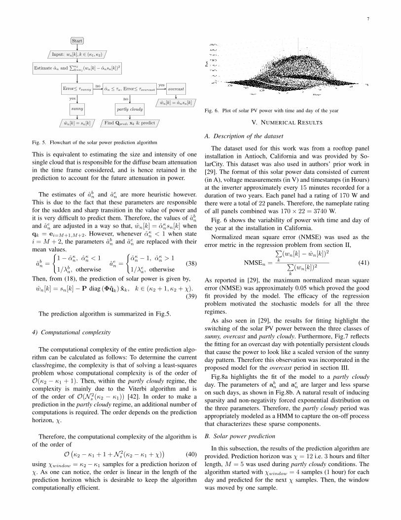
As also seen in [29], the results for fitting highlight theswitching of the solar PV power between the three classes ofsunny, overcast and partly cloudy. Furthermore, Fig.7 reflectsthe fitting for an overcast day with potentially persistent cloudsthat cause the power to look like a scaled version of the sunnyday pattern. Therefore this observation was incorporated in theproposed model for the overcast period in section III.

Fig.8a highlights the fit of the model to a partly cloudyday. The parameters of abn and aen are larger and less sparseon such days, as shown in Fig.8b. A natural result of inducingsparsity and non-negativity forced exponential distribution onthe three parameters. Therefore, the partly cloudy period wasappropriately modeled as a HMM to capture the on-off processthat characterizes these sparse components.

B. Solar power prediction

In this subsection, the results of the prediction algorithm areprovided. Prediction horizon was χ = 12 i.e. 3 hours and filterlength, M = 5 was used during partly cloudy conditions. Thealgorithm started with χwindow = 4 samples (1 hour) for eachday and predicted for the next χ samples. Then, the windowwas moved by one sample.

8

8 10 12 14 16 18

500

1,000

1,500

2,000

2,500

Time (hours)

Powe

r(W

)wn[k] sn[k] wn[k]

Fig. 7. Fit of the model to an overcast day

8 10 12 14 16 18

500

1,000

1,500

2,000

Time (hours)

Powe

r(W

)

wn[k] sn[k] wn[k]

(a) Fit to a partly cloudy day with sharp power fluctuations.

8 10 12 14 16 180

0.2

0.4

0.6

0.8

1

1.2

Time (hours)

Amplitu

de

zn[k] abn[k] aen[k]

(b) Parameters for a partly cloudy day with sharp power fluctuations

Fig. 8. Fitting a partly cloudy day

1) Metrics used for evaluation

The results are presented using both deterministic and prob-abilistic forecast metrics. In the deterministic setting, resultsare provided using the metrics of mean absolute percentageerror (MAPE), eabs[κτ ] and root mean squared error (RMSE),RMSE(kτ ) for the kτ -step prediction ,

eabs[κτ ] =

∑k,n

|wn[k]−wkτn [k]|wn[k]

∑k,n

1(42)

RMSE(kτ ) =

√√√√√√

∑k,n

(wn[k]− wkτn [k])2

∑k,n

1(43)

where wkτn [k] refers to the prediction at time k given wn[k−kτ ] and values before it.

In the probabilistic setting at each kτ -step prediction thereis a cumulative distribution function (CDF) Fwkτn [k](x) insteadof a point forecast wkτ [k]. Based on class of model chosenfor prediction, the CDF is determined as

Fwkτn [k](x) =

Φ(x−wkτn [k]

σs), sunny

∫ x0foc(x), overcast

∫ x0fi(x), i = 1, 2, . . . ,Ns, partly cloudy

(44)with Φ(.) denoting the CDF of a standard normal distribution,foc(x) and fi(x) are defined as in (17) and (24) respectively.The metrics used for evaluation are continuous rank probabil-ity score (CRPS) [43], reliability metric and score [44]. CRPSis defined for each kτ -step prediction as an average over allthe samples,

CRPS(kτ ) =

∑k,n

∫∞0

(Fwkτn [k](y)− u(y − wn[k])

)2dy

∑k,n

1

(45)where u(.) is the Heaviside step function. The CRPS evaluatesto mean squared error (MSE) when the forecast is determin-istic.

Reliability of a probabilistic forecasting method is a usefulmetric in understanding the proximity of the estimated CDFto the actual CDF of the data. Let a probability interval (PI),Iwkτn [k], be defined with an upper and lower bound such thatthe interval covers the observed value wn[k] with probability(1− b). Then, to calculate reliability, define

Rb(kτ ) =

∑k,n

I(wn[k]∈I

wkτn [k]

)∑k,n

1(46)

as the estimated probability of coverage where I(.) is anindicator function with value 1 if the observed sample belongsto the probability interval. Now, the probabilistic forecast ismore reliable if the quantity Rb

Rb(kτ ) , Rb(kτ )− (1− b) (47)is small.

Another metric used for evaluation is the score. This metricis helpful in determining the sharpness of the forecast proba-bility interval by imposing a penalty when an observation isoutside the interval, by a value proportional to the size of theinterval. If the upper and lower bounds of the PI are denotedas Uwkτn [k] and Lwkτn [k] respectively then score is defined as

Scorekτb

[k] =

9

8 10 12 14 16 18

−200

0

200

400

600

800

Time (hours)

Powe

r(W

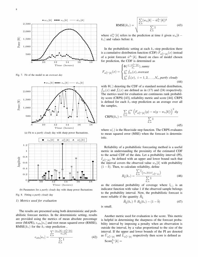
)50 percentile 90 percentile wn[k] wn[k]

Fig. 9. Plot of actual and predicted value with one-step prediction for daythat is overcast

Dwkτn [k] − 4(Lwkτn [k] − wn[k]

), wn[k] < Lwkτn [k]

Dwkτn [k], wn[k] ∈ Iwkτn [k]

Dwkτn [k] − 4(wn[k]− Uwkτn [k]

), wn[k] > Uwkτn [k]

(48)where

Dwkτn [k] , −2b(Uwkτn [k] − Lwkτn [k]

)(49)

The average score is,

Scoreb(kτ ) =

∑k,n

Scorekτb

[k]

∑k,n

1(50)

Lower values of the score indicate sharper and more reliableforecasts.

Performance of the prediction methods is analyzed usingaverage reliability and score defined as

Ravgb

=∑

kτ

Rb(kτ )/χ (51)

Scoreavgb

=∑

kτ

Scoreb(kτ )/χ (52)

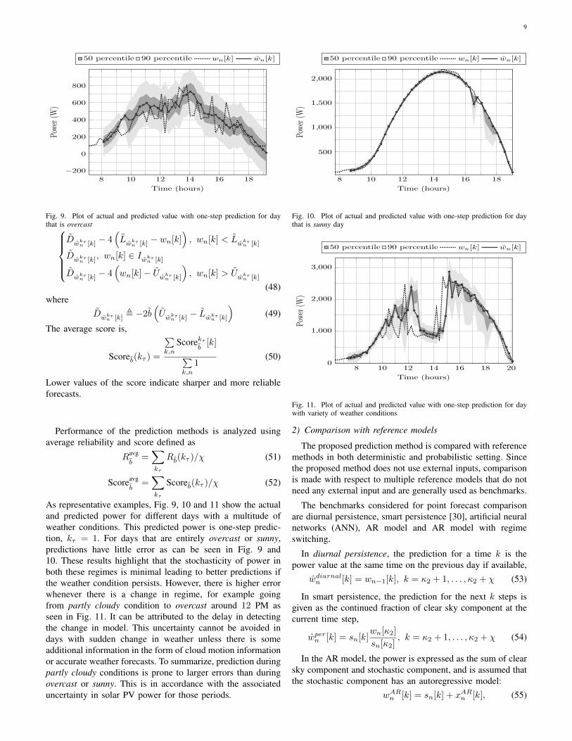
As representative examples, Fig. 9, 10 and 11 show the actualand predicted power for different days with a multitude ofweather conditions. This predicted power is one-step predic-tion, kτ = 1. For days that are entirely overcast or sunny,predictions have little error as can be seen in Fig. 9 and10. These results highlight that the stochasticity of power inboth these regimes is minimal leading to better predictions ifthe weather condition persists. However, there is higher errorwhenever there is a change in regime, for example goingfrom partly cloudy condition to overcast around 12 PM asseen in Fig. 11. It can be attributed to the delay in detectingthe change in model. This uncertainty cannot be avoided indays with sudden change in weather unless there is someadditional information in the form of cloud motion informationor accurate weather forecasts. To summarize, prediction duringpartly cloudy conditions is prone to larger errors than duringovercast or sunny. This is in accordance with the associateduncertainty in solar PV power for those periods.

8 10 12 14 16 18

500

1,000

1,500

2,000

Time (hours)

Powe

r(W

)

50 percentile 90 percentile wn[k] wn[k]

Fig. 10. Plot of actual and predicted value with one-step prediction for daythat is sunny day

8 10 12 14 16 18 200

1,000

2,000

3,000

Time (hours)

Powe

r(W

)

50 percentile 90 percentile wn[k] wn[k]

Fig. 11. Plot of actual and predicted value with one-step prediction for daywith variety of weather conditions

2) Comparison with reference models

The proposed prediction method is compared with referencemethods in both deterministic and probabilistic setting. Sincethe proposed method does not use external inputs, comparisonis made with respect to multiple reference models that do notneed any external input and are generally used as benchmarks.

The benchmarks considered for point forecast comparisonare diurnal persistence, smart persistence [30], artificial neuralnetworks (ANN), AR model and AR model with regimeswitching.

In diurnal persistence, the prediction for a time k is thepower value at the same time on the previous day if available,

wdiurnaln [k] = wn−1[k], k = κ2 + 1, . . . , κ2 + χ (53)

In smart persistence, the prediction for the next k steps isgiven as the continued fraction of clear sky component at thecurrent time step,

wpern [k] = sn[k]wn[κ2]

sn[κ2], k = κ2 + 1, . . . , κ2 + χ (54)

In the AR model, the power is expressed as the sum of clearsky component and stochastic component, and is assumed thatthe stochastic component has an autoregressive model:

wARn [k] = sn[k] + xARn [k], (55)

10

xARn [k] =

MAR∑

i=1

a[i]xARn [k − i] + εAR[k] (56)

In AR model with regime switching, it is assumed that each ofthe classes sunny, partly cloudy and overcast have stochasticcomponents with different coefficients corresponding to theAR model:

xARn [k] =

MARs∑i=1

as[i]xARn [k − i] + εARs [k], sunny

MARpc∑i=1

apc[i]xARn [k − i] + εARpc [k], partly cloudy

MARoc∑i=1

aoc[i]xARn [k − i] + εARoc [k], overcast

(57)In addition, the proposed method is also compared withthe artificial neural network (ANN) approach. Specifically,a non-linear autoregressive neural network (NARNET) [45]was used. These are essentially feed-forward networks withautoregressive nature:

wANNn [k] = sn[k] + xANNn [k], (58)

xANNn [k] =

L∑

i=1

Wi

P∑

j=1

f(βijx

ANNn [k − j] + θi

)(59)

2 hidden layers with 10 neurons each and a lag p = 15 wasused for the stochastic component, xANNn [k]. The activationfunction f(.) was tanh(x) = 2/(1 + exp (−2x))− 1.

For comparison in the probabilistic forecast setting, smartpersistence and AR models are used. In the smart persistenceapproach, it is assumed that the smart persistence forecastin (54) is the mean and the variance is estimated from thesamples used for forecasting. The distribution is assumed tobe Gaussian.

In both the AR model and the regime switching AR models,the point forecast value is the mean and the variance ofGaussian noise, εAR is estimated along with the coefficients.

3) ResultsAll the simulations were performed using one year of

training data and one year of testing data for validation.The programs were written using MATLAB and executed ona machine with Intel i7 processor with 8GB RAM and at2.2 GHz. Most of the training for estimation of parametersof HMM is done apriori making computational time of theproposed method very short since the Viterbi algorithm, whichis proven to be efficient [42] was used. The computational timespecifically depends on the acquisition time of samples in areal-time setting. In the simulation, since data was alreadyavailable, it took 4 milliseconds on an average to makepredictions for a horizon of 3 hours at 15 minute intervals,i.e. for 12 samples ahead.

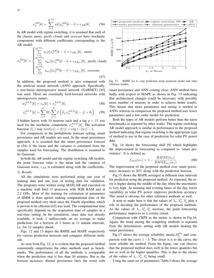
Figs. 12 and 13 depict the RMSE and MAPE respectivelyfor various prediction horizons and compares different meth-ods.

As seen from Fig. 12, it is evident that the proposed methodconsistently outperforms the other methods used as bench-marks. The performance of all the methods is comparablewhen the prediction step is less than 30 minutes. But as thehorizon increases, diurnal persistence fares the worst with

0.5 1 1.5 2 2.5 3

300

400

500

kτ in Hours

RMSE

(kτ)in

W

proposed method regime switching AR ARsmart persistence diurnal persistence ANN

Fig. 12. RMSE for kτ -step prediction using proposed model and otherreference models.

smart persistence and ANN coming close. ANN method faresbadly with respect to MAPE as shown in Fig. 13 indicatingthat architectural changes could be necessary with possiblymore number of neurons in order to achieve better results.This means that more parameters and tuning is needed inANNs whereas in comparison the proposed method uses fewerparameters and a low order model for prediction.

Both the types of AR models perform better than the naivebenchmarks as reported by other works. The regime switchingAR model approach is similar in performance to the proposedmethod indicating that regime switching is the appropriate typeof method to use in the case of prediction for solar PV powerdata.

Fig. 14 shows the forecasting skill [9] which highlightsthe improvement in forecasting as compared to ‘smart per-sistence’. It is defined as,

fskill(κτ ) = 1− RMSE(κτ )

RMSEper(κτ )(60)

The improvement of the proposed method over smart persis-tence increases to 20% along with the prediction horizon.

Fig.15 shows the MAPE averaged at different time intervalsfor prediction using the proposed method. As expected, the er-ror is higher during the middle of the day when the uncertaintyis very high. At morning and evening times of the day, lowervariability in solar PV power improves prediction accuracy.This trend is obvious for other reference methods as well.

A note to make here is that the values of λz, λba, λea play a

role in deciding the performance of the proposed methods.As the values of λz, λba, λ

ea increase, the point forecasting

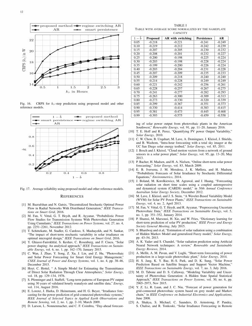
performance improves to a certain extent.Comparison with CRPS as the metric is shown in Fig.16.

Again, the trend among the competing methods is repeatedfrom the deterministic setting with AR models beating thesmart persistence.

Fig.17 shows the average reliability metric,Ravgb

and com-parison with the curve 1− b. The closer it is to the curve, themore reliable the method. From the figure, one can observethat the proposed method does well in the lower quantiles butnot so well in the higher quantiles. This is due to the choiceof the values of λz, λba, λ

ea being small.

Using the same set of parameters, Table.I shows the average

11

0.5 1 1.5 2 2.5 30.2

0.3

0.4

0.5

0.6

0.7

kτ in Hours

MAPE

(kτ)in

W

proposed method regime switching AR ARsmart persistence diurnal persistence ANN

Fig. 13. MAPE for kτ -step prediction using proposed model and otherreference models.

0.5 1 1.5 2 2.5 3

5

10

15

20

25

kτ in Hours

forecast

skill

proposed method regime switching AR AR

Fig. 14. Forecasting skill for kτ -step prediction using proposed model andother reference models as a percentage of improvement over smart persistence.

0.5 1 1.5 2 2.5 3

0.3

0.4

0.5

kτ in Hours

MAP

E(k

τ)in

W

7 AM-12 PM 12 PM-4 PM 4 PM-8 PM

Fig. 15. MAPE for kτ -step prediction at different times during a day usingproposed model.

score, Scoreavgb

normalized by the nameplate capacity. In termsof score, the proposed method outperforms all the other meth-ods considered. This is indicative of the fact that the forecastsfrom the proposed method are sharp and well calibrated ingeneral.

It is pertinent to discuss that λz, λba, λea and σs, σoc are

tuning parameters which affect the performance of the pro-posed method. Decreasing the values makes the predictionsless reliable and sharp but fares well when seen from theCRPS perspective. This is because CRPS only accounts forhow well the forecast probability intervals cover the observedvalue of power which means that larger the intervals (smallerλz, λ

ba, λ

ea), better is the CRPS. But the metrics of score and

reliability penalize wide intervals and therefore the methodfares better with smaller width of intervals (larger λz, λba, λ

ea

).

VI. DISCUSSION

The proposed method is better suited for shorter horizons i.e.less than 4 hours since persistence in weather condition isassumed. In the situation that no weather forecasts or otheradditional information is used, the performance of the pro-posed prediction algorithm is good and outperforms multiplebenchmark models. It was concluded that the regime switchingAR model is closest in performance to the proposed methodwhich shows the advantages of considering a regime switchingapproach since solar PV power data is non-stationary.

More importantly, the proposed model is stochastic and pro-vides probabilistic forecasts of power over the desired horizon.The performance of the proposed method can be adjusted bytuning the parameters λz, λba, λ

ea. Larger probability intervals

generated with smaller values of the parameters are moresuited when the evaluation metric is CRPS. Narrower intervalsare desirable for sharper and reliable forecasts. Based on thedemand of the application at hand, the forecasts can be suitablyadapted.

Sample future power scenarios can be produced by consid-ering all three stochastic models to be probable in the future.These scenarios are quite useful while solving stochasticoptimization problems such as designing a battery storagepolicy [46]. This is future work.

VII. CONCLUSIONS

A regime-switching process was proposed for the depictionand prediction of solar PV power. Stochastic models for differ-ent periods of sunny, overcast and partly cloudy were proposedalong with an online, computationally efficient algorithm forshort term probabilistic forecasts. The prediction algorithmwas shown to compare favorably with many reference models.It was also shown that the prediction algorithm is tunableand depending on the end goal, one can suitably adapt theperformance. Future work includes accounting for the spatialcorrelation in solar power at multiple locations through loworder models and extending the model to provide probabilisticforecasts at different locations simultaneously.

12

0.5 1 1.5 2 2.5 314

16

18

20

22

kτ in Hours

CRPS

(kτ)in

Wproposed method regime switching AR

AR smart persistence

Fig. 16. CRPS for kτ -step prediction using proposed model and otherreference models.

0.2 0.4 0.6 0.8

0.2

0.4

0.6

0.8

1− b

R

1− b proposed method

smart persistence regime switching ARAR

Fig. 17. Average reliability using proposed model and other reference models.

REFERENCES

[1] M. Bazrafshan and N. Gatsis, “Decentralized Stochastic Optimal PowerFlow in Radial Networks With Distributed Generation,” IEEE Transca-tions on Smart Grid, 2016.

[2] M. Fan, V. Vittal, G. T. Heydt, and R. Ayyanar, “Probabilistic PowerFlow Studies for Transmission Systems With Photovoltaic GenerationUsing Cumulants,” IEEE Transactions on Power Systems, vol. 27, no. 4,pp. 2251–2261, November 2012.

[3] T. Schittekatte, M. Stadler, G. Cardoso, S. Mashayekh, and N. Sankar,“The impact of short-term stochastic variability in solar irradiance onoptimal microgrid design,” IEEE Transcations on Smart Grid, 2016.

[4] Y. Ghiassi-Farrokhfal, S. Keshav, C. Rosenberg, and F. Ciucu, “Solarpower shaping: An analytical approach,” IEEE Transactions on Sustain-able Energy, vol. 6, no. 1, pp. 162–170, January 2015.

[5] C. Wan, J. Zhao, Y. Song, Z. Xu, J. Lin, and Z. Hu, “Photovoltaicand Solar Power Forecasting for Smart Grid Energy Management,”CSEE Journal of Power and Energy Systems, vol. 1, no. 4, pp. 38–46,December 2015.

[6] Hoyt. C. Hottel, “ A Simple Model for Estimating the Transmittanceof Direct Solar Radiation Through Clear Atmospheres,” Solar Energy,vol. 18, pp. 129–134, 1976.

[7] S. Pfenninger and I. Staffell, “Long-term patterns of European PV outputusing 30 years of validated hourly reanalysis and satellite data,” Energy,vol. 114, August 2016.

[8] E. Lorenz, J. Hurka, D. Heinemann, and H. G. Beyer, “Irradiance fore-casting for the power prediction of grid-connected photovoltaic systems,”IEEE Journal of Selected Topics in Applied Earth Observations andRemote Sensing, vol. 2, no. 1, pp. 2–10, March 2009.

[9] D. Larson, L. Nonnenmacher, and C. F. Coimbra, “Day-ahead forecast-

TABLE ITABLE WITH AVERAGE SCORE NORMALIZED BY THE NAMEPLATE

CAPACITY

1− b Proposed AR with switching Persistence AR0.05 -0.218 -0.221 -0.241 -0.2490.10 -0.219 -0.212 -0.242 -0.2390.15 -0.207 -0.205 -0.230 -0.2320.20 -0.208 -0.201 -0.232 -0.2270.25 -0.200 -0.198 -0.225 -0.2240.30 -0.203 -0.198 -0.228 -0.2240.35 -0.199 -0.200 -0.226 -0.2240.40 -0.203 -0.204 -0.231 -0.2280.45 -0.207 -0.209 -0.235 -0.2330.50 -0.209 -0.218 -0.240 -0.2400.55 -0.214 -0.228 -0.249 -0.2490.60 -0.221 -0.242 -0.256 -0.2610.65 -0.228 -0.257 -0.267 -0.2750.70 -0.241 -0.277 -0.282 -0.2930.75 -0.263 -0.300 -0.309 -0.3130.80 -0.273 -0.330 -0.320 -0.3390.85 -0.299 -0.367 -0.351 -0.3730.90 -0.330 -0.414 -0.383 -0.4150.95 -0.381 -0.473 -0.445 -0.4680.99 -0.393 -0.575 -0.459 -0.558

ing of solar power output from photovoltaic plants in the AmericanSouthwest,” Renewable Energy, vol. 91, pp. 11–20, January 2016.

[10] T. E. Hoff and R. Perez, “Quantifying PV power Output Variability,”Solar Energy, 2010.

[11] C. W. Chow, B. Urquhart, M. Lave, A. Dominguez, J. Kleissl, J. Shields,and B. Washom, “Intra-hour forecasting with a total sky imager at theUC San Diego solar energy testbed,” Solar Energy, vol. 85, 2011.

[12] J. Bosch and J. Kleissl, “Cloud motion vectors from a network of groundsensors in a solar power plant,” Solar Energy, vol. 95, pp. 13–20, May2013.

[13] P. Bacher, H. Madsen, and H. A. Nielsen, “Online short-term solar powerforecasting,” Solar Energy, vol. 83, March 2009.

[14] E. B. Iversena, J. M. Moralesa, J. K. Møllera, and H. Madsen,“Probabilistic Forecasts of Solar Irradiance by Stochastic DifferentialEquations,” Environmetrics, 2014.

[15] J. Boland, M. Korolkiewicz, M. Agrawal, and J. Huang, “Forecastingsolar radiation on short time scales using a coupled autoregressiveand dynamical system (CARDS) model,” in 50th Annual ConferenceAustralian Solar Energy Society, December 2012.

[16] M. Lave, J. Kleissl, and J. S. Stein, “A Wavelet-Based Variability Model(WVM) for Solar PV Power Plants,” IEEE Transactions on SustainableEnergy, vol. 4, no. 2, April 2013.

[17] M. Fan, V. Vittal, G. T. Heydt, and R. Ayyanar, “Preprocessing UncertainPhotovoltaic Data,” IEEE Transactions on Sustainable Energy, vol. 5,no. 1, pp. 351–352, January 2014.

[18] P. Shamsi, M. Marsousi, H. Xie, and W. Fries, “Dictionary learning forshort-term prediction of solar PV production,” IEEE Power and EnergySociety General Meeting, July 2015.

[19] S. Bhardwaj and et.al, “Estimation of solar radiation using a combinationof Hidden Markov Model and generalized Fuzzy model,” Solar Energy,pp. 43–54, 2013.

[20] A. K. Yadav and S. Chandel, “Solar radiation prediction using ArtificialNeural Network techniques: A review,” Renewable and SustainableEnergy Reviews, 2014.

[21] A. Mellit, A. M. Pavan, and V. Lughi, “Short-term forecasting of powerproduction in a large-scale photovoltaic plant,” Solar Energy, 2014.

[22] H. S. Jang, K. Y. Bae, H.-S. Park, and D. K. Sung, “Solar PowerPrediction Based on Satellite Images and Support Vector Machine,”IEEE Transactions on Sustainable Energy, vol. 7, no. 3, July 2016.

[23] M. D. Tabone and D. S. Callaway, “Modeling Variability and Uncer-tainty of Photovoltaic Generation: A Hidden State Spatial StatisticalApproach,” IEEE Transactions on Power Systems, vol. 30, no. 6, pp.2965–2973, Nov 2015.

[24] Y. Z. Li, R. Luan, and J. C. Niu, “Forecast of power generation forgrid-connected photovoltaic system based on grey model and Markovchain,” in IEEE Conference on Industrial Electronics and Applications,June 2008.

[25] A. Shakya, S. Michael, C. Saunders, D. Armstrong, P. Pandey,S. Chalise, and R. Tonkoski, “Solar Irradiance Forecasting in Remote

13

Microgrids Using Markov Switching Model,” IEEE Transactions onSustainable Energy, vol. 8, no. 3, July 2017.

[26] Z. Ren, W. Yan, X. Zhao, W. Li, and J. Yu, “Chronological Probabil-ity Model of Photovoltaic Generation,” IEEE Transactions on PowerSystems, vol. 29, no. 3, 2014.

[27] M. J. Sanjari and H. B. Gooi, “Probabilistic Forecast of PV PowerGeneration Based on Higher Order Markov Chain,” IEEE Transactionson Power Systems, vol. 32, no. 4, July 2017.

[28] J.D.Hamilton, “Regime-switching models,” Macroeconometrics andtime series analysis, 2010.

[29] R. Ramakrishna and A. Scaglione, “A Compressive Sensing Frameworkfor the analysis of Solar Photo-Voltaic Power,” in Conference Record ofthe Fiftieth Asilomar Conference on Signals, Systems and Computers,2016, pp. 308–312.

[30] H. T. Pedro and C. F. Coimbra, “Assessment of forecasting techniquesfor solar power production with no exogenous inputs,” Solar Energy,vol. 86, no. 7, pp. 2017–2028, May 2012.

[31] Gilbert. M. Masters, Renewable and Efficient Electric Power Systems.Wiley, 2004.

[32] M. Abramowitz and I. Stegun, Handbook of Mathematical Functions.Dover Publications, 1965.

[33] A. Kankiewicz, M. Sengupta, and D. Moon, “Observed impacts oftransient clouds on utility-scale PV fields,” in ASES National SolarConference, 2010.

[34] A. E. Curtright and J. Apt, “The Character of Power Output from Utility-Scale Photovoltaic Systems,” Progress in Photovoltaics: Research andApplications, vol. 16, pp. 241–247, September 2007.

[35] Alan V. Oppenheim and Ronald W. Schafer, Discrete-Time SignalProcessing. Pearson, 2010.

[36] Ivana Tosic and Pascal Frossard, “Dictionary learning,” IEEE SignalProcessing Magazine, pp. 27–38, March 2011.

[37] B. Mailhe, S. Lesage, R. Gribonval, F. Bimbot, and P. Vandergheynst,“Shift- invariant dictionary learning for sparse representations: Extend-ing K-SVD,” in European Signal Processing Conference, vol. 4, 2008.

[38] Joel A. Tropp and Stephen J.Wright, “Computational Methods for SparseSolution of Linear Inverse Problems,” Proceedings of the IEEE, vol. 98,no. 6, pp. 948–958, June 2010.

[39] R. H. Inman, H. T. Pedro, and C. F. Coimbra, “Solar forecasting methodsfor renewable energy integration,” Progress in Energy and CombustionScience, 2013.

[40] F. Jelinek, “Continuous Speech Recognition by Statistical Methods,”Proceedings of the IEEE, vol. 64, no. 4, pp. 532–556, April 1976.

[41] B. H. Juang and L. Rabiner, “The Segmental K-Means Algorithm forEstimating Parameters of Hidden Markov Models,” IEEE Transactionson Acoustics, Speech, and Signal Processing, vol. 38, no. 9, pp. 1639–1641, September 1990.

[42] G.D.Forney, “The Viterbi algorithm,” Proceedings of the IEEE, vol. 61,no. 3, pp. 268–278, March 1973.

[43] T. Gneiting, F. Balabdaoui, and A. E. Raftery, “Probabilistic forecasts,calibration and sharpness,” Journal of the Royal Statistical Society:Series B (Statistical Methodology, vol. 69, no. 243-268, 2007.

[44] C. Wan, Z. Xu, P. Pinson, Z. Y. Dong, and K. P. Wong, “OptimalPrediction Intervals of Wind Power Generation,” IEEE Transactions onPower Systems, vol. 29, no. 3, May 2014.

[45] J. T. Connor, R. D. Martin, and L. E. Atlas, “Recurrent Neural Networksand Robust Time Series Prediction ,” IEEE Transactions on NeuralNetworks, vol. 5, no. 2, March 1994.

[46] W. B. Powell and S. Meisel, “Tutorial on Stochastic Optimization inEnergy—Part I: Modeling and Policies,” IEEE Transactions on PowerSystems, vol. 31, no. 2, pp. 1459–1467, March 2016.