A Step-By-Step Procedure to The

Numerical Solution for

Time-Dependent Partial

Derivative Equations in Three

Spatial Dimensions

Xi WangXinyan Lin

Supervisor: Jan RomanSchool of Education, Culture and Communication

Malardalen University2012.09.17

Declaration

We declare that this thesis was composed by ourselves and that the work contained therein isour own, except where explicitly stated otherwise in the text.

(Xi WangXinyan Lin)

2

Acknowledgement

To our supervisor Jan Roman who is the lecturer of Analytical Finance I and II, assistant vicepresident and head of market risk in Swedbank in Sweden. First of all, thanks for giving us sucha challengeable topic. Secondly, we appreciate your invaluable experience, patience, encourage-ment and continuous support. Otherwise, this paper would not have been achieved so far.Also, thanks to two PHD students: Karl Lundengard and Christopher Engstrom in MalardalenUniversity, they are also the lecturers in the course Applied Matrix Analysis and NumericalMethod with Matlab. With their experiences and knowledge, the matrices in programmingpart have been dealt with successfully.

3

Abstract

Derivative market has been trading for quite a long time, like options, futures. Meanwhile,interest rate derivative market is the biggest derivative market among the others in the world.In recent years, interest rate derivative arises much concern for various purposes. For example,an investor from one country may have access to getting involved in some derivatives in anothercountry by exposing himself to the exchange rate. However, in this situation, simulation meth-ods to value such derivative might seem inadequate. On the other hand, numerical methods,which have done remarkable job when applied to the valuation, therefore, are strongly recom-mended in the academic community. This paper consolidates insights from another seminarpaper [3] which proposes a Partial Differential Equation (PDE) approach to price cross-currencyinterest rate derivatives in terms of three correlated processes, uses finite difference methodsfor the spatial discretization of the PDE, and proves that the Alternative Direction Implicitis the most efficient method to solve such PDE. However, no detailed procedure is shown tosolve the time-dependent parabolic PDE in three spatial dimensions. Thus, our work focuseson providing step-by-step instructions that enable the reader to follow to solve the parabolicPDE by finite difference method. Meanwhile, this paper is a guide for readers to see how thePDE is applicable to general realistic financial problems.

4

Contents

Abstract 4

List of Figures 6

1 Introduction 7

2 Derivation of the PDE 82.1 Introducing the three dynamic processes and the functions . . . . . . . . . . . . . 82.2 Ito‘s lemma . . . . . . . . . . . . . . . . . . . . . . . . . . . . . . . . . . . . . . . 8

3 The Alternative Direction Implicit Scheme 103.1 finite differences . . . . . . . . . . . . . . . . . . . . . . . . . . . . . . . . . . . . 103.2 Alternating Direction Implicit Method . . . . . . . . . . . . . . . . . . . . . . . . 11

4 The HV scheme 144.1 Discover splitting scheme . . . . . . . . . . . . . . . . . . . . . . . . . . . . . . . 14

5 Boundary conditions for the ADI method 16

6 Thomas Algorithm 18

7 Summary 19

8 Future Work 20

9 Bibliography 21

A First Appendix 22

B Second Appendix 23

C ”Fixed notional” method 24

D Codes in Matlab 25

5

List of Figures

3.1 The split in three dimensions . . . . . . . . . . . . . . . . . . . . . . . . . . . . . 12

5.1 Illustration on the boundary conditions and the solution area . . . . . . . . . . . 17

6.1 Illustration on Diagonal Matrix transformation by Thomas algorithm . . . . . . . 18

6

Chapter 1

Introduction

In this paper, we investigate the cross-currency swap by using the PDE approach. Particularly,it is floating to floating cross-currency swap which involves foreign exchange rate and the interestrates for two currencies. The current standard modeling of such products consist of two one-factor Gaussian models for the term structures and one-factor log-normal model for the spotFX rate [3][10]. However, these three time-dependent variables construct a three dimensionproblem. Generally, such PDE is considered to be a massively computational challenge if it issolved straightforward. Therefore, we also investigate the efficient and well-known AlternativeDirection Implicit (ADI) method to solve the PDE.In this paper we avoid to discuss the models and the parameters in the models, but only focuson the how the PDE approach is applied to find the value of such derivatives. The outline ofthe rest of this paper is arranged as follows. In section 2, we present the models and show howthe PDE is derived. Section 3 and 4, Alternative Direction Implicit method and the splittingmethod are demonstrated, so that making a bunch of equations into a nice and acceptableaccuracy scheme which results in a convenience computer programming system. Section 5 and6; generally give a short introduction to the boundary conditions and the Thomas Algorithm.Section 7 and 8 give a short summary and future work.

7

Chapter 2

Derivation of the PDE

2.1 Introducing the three dynamic processes and the func-tions

Let u(s, rd, rf , t) denote the domestic value function of a security, where s is spot foreignexchange rate; rd,rf are the domestic and foreign short rate respectively [3].Assume the spot FX as follows [9]:

ds(t) = (rd(t)− rf (t))s(t)dt+ γ(t, s(t))s(t)dWs(t) (2.1.1)

where Ws(t) is a Brownian motion. rd and rf follow the mean-reverting Hull-White model andhave the following dynamics [9]:

drd(t) = (θd(t)− κd(t)rd(t))dt+ σd(t)dWd(t) (2.1.2)

drf (t) = (θf (t)− κf (t)rf (t))dt− ρs,f (t)σf (t)γ(t, s(t))dt+ σf (t)dWf (t) (2.1.3)

where deterministic functions κi(t) and σi(t), with i = d, f , are the mean reversion rates and thevolatility functions. Deterministic function θi(t) is a function of time determining the averagedirection in which ri moves. dWd(t) and dWf (t) are the other Brownian motions with respectto rd and rf .The ”quanto” drift adjustment, −ρs,fσf (t)γ(t, s(t)) for drf (t) comes from changing the measurefrom the foreign risk-neutral measure to the domestic risk neutral one. γ(t, s(t)) is the localvolatility function for the spot FX rate has the functional form [9]

γ(t, s(t)) = ξ(t)

(s(t)

L(t)

)ζ(t)−1(2.1.4)

where ξ(t) is the relative volatility function, ζ(t) is the time-dependent constant elasticity ofvariance (CEV) parameter and L(t) is a time-dependent scaling constant [3].

2.2 Ito‘s lemma

Because the normalized price process of any security is a martingale under the domestic risk-neutral measure, it is easy to apply the Ito‘s lemma and simply set the drift term to be zero.Ito‘s lemma gives:

du =∂u

∂tdt+

∂u

∂sds+

∂u

∂rddrd +

∂u

∂rfdrf +

1

2

∂2u

∂s2ds2 +

1

2

∂2u

∂r2ddr2d +

1

2

∂2u

∂r2fdr2f

+∂2u

∂rd∂sdsdrd +

∂2u

∂rf∂sdsdrf +

∂2u

∂rf∂rddrddrf (2.2.1)

8

Substituting the dynamics gives:

du =∂u

∂tdt+

∂u

∂s((rd(t)− rf (t))s(t)dt+ γ(t, s(t))s(t)dWs(t))

+∂u

∂rd((θd(t)− κd(t))rd(t)dt+ σd(t)dWd(t))

+∂u

∂rf((θf (t)− κf (t)rf (t))dt− ρfs(t)σf (t)γ(t, s(t))dt+ σf (t)dWf (t))

+1

2

∂2u

∂s2(γ2(t, s(t))s2(t)dt) +

1

2

∂2u

∂r2d(σ2d(t)dt) +

1

2

∂2u

∂r2f(σ2f (t)dt)

+∂2u

∂s∂rd(ρs,dσd(t)γ(t, s(t))sdt) +

∂2u

∂s∂rf(ρs,fσf (t)γ(t, s(t))sdt)

+∂2u

∂rd∂rf(ρd,fσd(t)σf (t)dt) (2.2.2)

Rearrange the above equation and group the - dt terms, because of the martingale property, bysetting these terms equal to zero the PDE is derived as:

∂u

∂t+ (rd − rf )s

∂u

∂s+ (θd(t)− κd(t)rd)

∂u

∂rd

+ (θf (t)− κf (t)rf − ρf,sσf (t)γ(t, s(t)))∂u

∂rf

+1

2γ2(t, s(t))s2

∂2u

∂s2+

1

2σ2d(t)

∂2u

∂r2d+

1

2σ2f (t)

∂2u

∂r2f

+ ρs,dσd(t)γ(t, s(t))s∂2u

∂s∂rd+ ρs,fσf (t)γ(t, s(t))s

∂2u

∂s∂rf+ ρd,fσd(t)σf (t)

∂2u

∂rd∂rf− rdu

= 0 (2.2.3)

9

Chapter 3

The Alternative DirectionImplicit Scheme

3.1 finite differences

In the discretization, the first and second derivative terms can all be approximated by thecentral difference method as presented following [3][7]:

∂u

∂s≈umi+1,j,k − umi−1,j,k

24s,∂2u

∂s2≈umi+1,j,k − 2umi,j,k + umi−1,j,k

4s2(3.1.1)

Similarly,∂u

∂rd≈umi,j+1,k − umi,j−1,k

24rd,∂2u

∂r2d≈umi,j+1,k − 2umi,j,k + umi,j−1,k

4r2d(3.1.2)

∂u

∂rf≈umi,j,k+1 − umi,j,k−1

24rf,∂2u

∂r2f≈umi,j,k+1 − 2umi,j,k + umi,j,k−1

4r2f(3.1.3)

∂u

∂t≈umi,j,k − u

m−1i,j,k

4t(3.1.4)

While the cross-derivative terms are approximated by a four-point finite difference:

∂2u

∂rd∂s=umi+1,j+1,k + umi−1,j−1,k − umi−1,j+1,k − umi+1,j−1,k

44s4rd(3.1.5)

∂2u

∂rf∂s=umi+1,j,k+1 + umi−1,j,k−1 − umi−1,j,k+1 − umi+1,j,k−1

44s4rf(3.1.6)

∂2u

∂rd∂rf=umi,j+1,k+1 + umi,j−1,k−1 − umi,j−1,k+1 − umi,j+1,k−1

44rf4rd(3.1.7)

Where, m denotes the time index, and i, j, k denote the s−, r−d , r−f direction.Because we solve the PDE backward in time, by changing variable τ = Tend−Tstart [3] the abovedifferential equation 2.2.3 can be rewritten as following when substitute the finite differences in

10

the corresponding terms:

(rd − rf )s

(umi+1,j,k − umi−1,j,k

24s

)+

1

2γ2(t, s(t))s2

(umi+1,j,k − 2umi,j,k + umi−1,j,k

4s2

)+ (θd(t)− κd(t)rd)

(umi,j+1,k − umi,j−1,k

24rd

)+

1

2σ2d(t)

(umi,j+1,k − 2umi,j,k + umi,j−1,k

4r2d

)+ (θf (t)− κf (t)rf − ρf,sσf (t)γ(t, s(t)))

(umi,j,k+1 − umi,j,k−1

24rf

)+

1

2σ2f (t)

(umi,j,k+1 − 2umi,j,k + umi,j,k−1

4r2f

)

+ ρs,dσd(t)γ(t, s(t))s

(umi+1,j+1,k + umi−1,j−1,k − umi−1,j+1,k − umi+1,j−1,k

44s4rd

)+ ρs,fσf (t)γ(t, s(t))s

(umi+1,j,k+1 + umi−1,j,k−1 − umi−1,j,k+1 − umi+1,j,k−1

44s4rf

)+ ρd,fσd(t)σf (t)

(umi,j+1,k+1 + umi,j−1,k−1 − umi,j−1,k+1 − umi,j+1,k−1

44rf4rd

)− rdu

=

(umi,j,k − u

m−1i,j,k

4τ

)(3.1.8)

Rearrange in terms of the directions i−, j−, k−:((rd − rf )s

24s+γ2(t, s(t))s2

24s2

)umi+1,j,k +

(− (rd − rf )s

24s+γ2(t, s(t))s2

24s2

)umi−1,j,k

− γ2(t, s(t))s2

4s2umi,j,k +

(θd(t)− κd(t))rd

24rd+σ2d(t)

24r2d

)umi,j+1,k

+

(−θd(t)− κd(t))rd

24rd+σ2d(t)

24r2d

)umi,j−1,k −

σ2d(t)

4r2dumi,j,k

+

(θf (t)− κf (t)rf − ρf,sσf (t)γ(t, s(t))

24rf+σ2f (t)

24r2f

)umi,j,k+1 −

σ2f (t)

4r2fumi,j,k

+

(−θf (t)− κf (t)rf − ρf,sσf (t)γ(t, s(t))

24rf+σ2f (t)

24r2f

)umi,j,k−1

+ρs,dσd(t)γ(t, s(t))s

44s4rd(umi+1,j+1,k + umi−1,j−1,k − umi−1,j+1,k − umi+1,j−1,k

)+

ρs,fσf (t)γ(t, s(t))s

44s4rf(umi+1,j,k+1 + umi−1,j,k−1 − umi−1,j,k+1 − umi+1,j,k−1

)+

ρd,fσd(t)σf (t)

44rf4rd(umi,j+1,k+1 + umi,j−1,k−1 − umi,j−1,k+1 − umi,j+1,k−1

)− rdu

=umi,j,k − u

m−1i,j,k

4τ(3.1.9)

3.2 Alternating Direction Implicit Method

The basic idea behind the ADI method is to split the finite difference equations into differentdirections. Since in our case, the three dimensions form a cube for every time step, Figure 3.1demonstrates the idea.For each split, only one direction is taken implicit. As the procedure continues, the exactsolution will be found. From the finite difference method, Equation 3.1.9 can be written in the

11

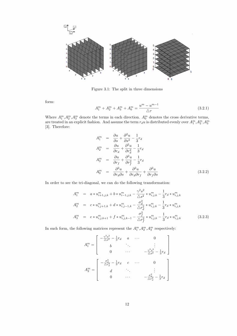
Figure 3.1: The split in three dimensions

form:

Am1 +Am2 +Am3 +Am0 =um − um−1

4τ(3.2.1)

Where Am1 ,Am2 ,Am3 denote the terms in each direction. Am0 denotes the cross derivative terms,are treated in an explicit fashion. And assume the term rdu is distributed evenly overAm1 ,Am2 ,Am3[3]. Therefore:

Am1 =∂u

∂s+∂2u

∂s2− 1

3rd

Am2 =∂u

∂rd+∂2u

∂r2d− 1

3rd

Am3 =∂u

∂rf+∂2u

∂r2f− 1

3rd

Am0 =∂2u

∂rd∂s+

∂2u

∂rd∂rf+

∂2u

∂rf∂s(3.2.2)

In order to see the tri-diagonal, we can do the following transformation:

Am1 = a ∗ umi+1,j,k + b ∗ umi−1,j,k −γ2s2

4s2∗ umi,j,k −

1

3rd ∗ umi,j,k

Am2 = c ∗ umi,j+1,k + d ∗ umi,j−1,k −σ2d

4r2d∗ umi,j,k −

1

3rd ∗ umi,j,k

Am3 = e ∗ umi,j,k+1 + f ∗ umi,j,k−1 −σ2f

4r2f∗ umi,j,k −

1

3rd ∗ umi,j,k (3.2.3)

In such form, the following matrices represent the Am1 ,Am2 ,Am3 respectively:

Am1 =

−γ

2s2

4s2 −13rd a · · · 0

b. . .

...

0 · · · −γ2s2

4s2 −13rd

Am2 =

− σ2

d

4r2d− 1

3rd c · · · 0

d. . .

...

0 · · · − σ2d

4r2d− 1

3rd

12

Am3 =

− σ2

f

4r2f− 1

3rd e · · · 0

f. . .

...

0 · · · − σ2f

4r2f− 1

3rd

Where

a =(rd − rf )s

24s+

γ2s2

24s2

b = − (rd − rf )s

24s+

γ2s2

24s2

c =(θd − κdrd)

24rd+

σ2d

24r2d

d = − (θd − κdrd)24rd

+σ2d

24r2d

e =(θf − κfrf − ρs,fσfγ)

24rf+

σ2f

24r2f

f = − (θf − κfrf − ρs,fσfγ)

24rf+

σ2f

24r2f

13

Chapter 4

The HV scheme

The Hundsdorfer and Verwer (HV) [5] splitting scheme as suggested in [3] approximates theexact solution Um:

V0 = Um−1 +4(Am−1Um−1 + gm−1)

(I − 124τA

mi )Vi = Vi−1 − 1

24τAm−1i + 1

24τ(gmi − gm−1i ), i = 1, 2, 3

V0 = V0 + 124τ(AmV3 −Am−1Um−1) + 1

24τ(gm − gm−1)

(I − 124τA

mi )Vi = Vi−1 − 1

24τAmi V3, i = 1, 2, 3

Um = V3.

Here the vector gm is the boundary conditions for the corresponding directions, will be discussedin the later section. In our case, the boundary conditions form a cube. Besides, from now on,the A matrices are defined in a slightly different manner because of the computational andprogramming purpose; they are presented in the Appendix A.

4.1 Discover splitting scheme

Applying the Douglas [4] ADI scheme to the equation 3.2.1, obtain a first evaluate of thesolution at time m+ 1 by taking implicitly half of the A1 :

1

2A1(um+ 1

3 + um) +A2um +A3u

m +A0um =

um+ 13 − um

4τ(4.1.1)

Then, taking half of the A2 ,A3 respectively,

1

2A1(um+ 1

3 + um) +1

2A2(um+ 2

3 + um) +A3um +A0u

m =um+ 2

3 − um

4τ(4.1.2)

1

2A1(um+ 1

3 + um) +1

2A2(um+ 2

3 + um) +1

2A3(um+1 + um) +A0u

m =um+1 − um

4τ(4.1.3)

The intermediate values um+ 13 , um+ 2

3 can be eliminated. The reader is strongly recommendedto the reference [4] for detailed elimination procedures.For splitting purpose, the above can be rewritten as:

(I − 1

24τA1)um+ 1

3 = um +4τ(A2um +A3u

m +A0um) +

1

24τA1u

m (4.1.4)

(I − 1

24τA2)um+ 2

3 = um +1

24τA1(um+ 1

3 + um) +1

2A2u

m +A3um +A0u

m (4.1.5)

(I − 1

24τA3)um+1 = um +

1

24τA1(um+ 1

3 + um) +1

2A2(um+ 2

3 + um)

+1

2A3u

m +A0um (4.1.6)

14

For the programming purpose, the above can be sorted as:{V0 = Um +4τ(AmUm)

(I − 124τAi)Vi = Vi−1 − 1

24τAm−1i Um i = 1, 2, 3

(4.1.7)

Where Am is the sum of the A0, A1, A2, A3, and Vi with i = 1, 2, 3 is corresponding to um+ 13 ,

um+ 23 , um+1 in equation 4.1.4, 4.1.5, 4.1.6.

The scheme 4.1.7 is so called Douglas-Rachford method (DR method). The HV method isderived in a similar manner, while, taking more steps to stabilize the solution on each stepto ensure the final solution, can be viewed as an extension of DR method. In 4.1.4, thereare actually I + 1 equations, but only three unknown variables for each equation regardless

the boundary conditions, namely um+ 1

3

i−1,j,k, um+ 1

3

i,j,k , um+ 1

3

i+1,j,k. Similarly, in j and k directions,

um+ 2

3

i,j−1,k,um+ 2

3

i,j,k ,um+ 2

3

i,j+1,k,um+1i,j,k−1,um+1

i,j,k ,um+1i,j,k+1 are unknown. As stated earlier, A1, A2, A3 are

tri-diagonal matrices, therefore, the equations 4.1.4, 4.1.5, 4.1.6 can be expressed below:

(I − 1

24τA1

)

um+ 1

3

1,j,k

um+ 1

3

2,j,k

um+ 1

3

3,j,k

um+ 1

3

4,j,k...

um+ 1

3

i,j,k

= [ω1]

(I − 1

24τA2

)

um+ 2

3

i,1,k

um+ 2

3

i,2,k

um+ 2

3

i,3,k

um+ 2

3

i,4,k...

um+ 2

3

i,j,k

= [ω2]

(I − 1

24τA3

)

um+1i,j,1

um+1i,j,2

um+1i,j,3

um+1i,j,4...

um+1i,j,k

= [ω3]

ω1 is a (I + 1)× 1 dimension vector with components:

ω1 = um +4τ(A2um +A3u

m +A0um) +

1

24τA1u

m

Similar to ω2 and ω3 , but the dimensions are (J + 1)× 1 and (K + 1)× 1 respectively.

ω2 = um +1

24τA1(um+ 1

3 + um) +1

2A2u

m +A3um +A0u

m

ω3 = um +1

24τA1(um+ 1

3 + um) +1

2A2(um+ 2

3 + um) +1

2A3u

m +A0um

15

Chapter 5

Boundary conditions for the ADImethod

In numerical method, it is unnecessary to construct the whole universe; therefore, work must bedone to decide the region we are only interested in. Proper boundary conditions can significantlyreduce the computation time and increase the accuracy of the results. In other words, theboundary condition is one of the most significant parts of such PDE functions. There aremany boundary conditions can be applied to PDE function, for example, Dirichlet boundaryconditions, Neumann boundary conditions and mixed boundary conditions. Nevertheless, someboundary conditions can be very complicated. For the Neumann boundary conditions, insteadof having fixed values on the bonded surfaces, it uses the derivatives. For instance, in the s−

direction, the second-order one-sided approximation gives the following:

∂u

∂s≈

4 ∗ umi+1,j,k − umi+2,j,k − 3 ∗ umi,j,k24s

= g1 forward

∂u

∂s≈umi−2,j,k − 4 ∗ umi−1,j,k + 3 ∗ umi,j,k

24s= g2 backward

The start and end surfaces are um0,j,k, umI,j,k and then, the um0,j,k and umI,j,k are solved from theforward and backward differences which will result in the different coefficients in the matrix onthe left hand side of the equation as well as the right hand side. This boundary condition ismore complicated in implementations. We will continue to discuss this topic in the next paper,where we will do the calibrations and show different boundary conditions result in comparableresults. For now, in this paper, we simply apply the Dirichlet boundary conditions where thereare fixed values on the end surfaces. This type of the boundary condition takes the values onthe boundary points as known, but only changes the right hand side of the equation when theboundary conditions are considered.

F1 − g1F2

F3

...

...Fn−1Fn − gn

To be more explicit, in our case, the boundary conditions are surfaces. Figure 5.1 belowillustrates the boundaries and the area we are really concern about which is indicated by thered hypercube. Readers can get helps to understand the boundary conditions by having a lookat the [1, 2, 6] in the reference.

16

Figure 5.1: Illustration on the boundary conditions and the solution area

17

Chapter 6

Thomas Algorithm

HV scheme has made the algorithm clear enough to solve the Um, but since the algorithminvolves solving a large number of systems of equations which may cause difficulties in theimplementation. Fortunately, knowing that A1, A2, A3 are three tri-diagonal matrices, theThomas algorithm [11] has been invented and recommended to help us to do the job. The basicidea behind the algorithm is substitution which will result in a new tri-diagonal matrix. Ofcourse, the vector on the right hand side of the equation will be substituted as well. However,the advantage is, the elements in sub-diagonal in new tri-diagonal matrix are zeros, and thediagonal elements are ones. Figure 6.1 illustrates how the diagonal matrix is transformed usingthe Thomas algorithm.

Figure 6.1: Illustration on Diagonal Matrix transformation by Thomas algorithm

18

Chapter 7

Summary

Up until here we have made complete procedures to the numerical method for three dimensionalpartial derivative equations. As can be seen, such problems could be extremely complex. Thematrices we illustrated on this paper only reflect the general forms. When the indices areconsidered, we are actually dealing with hundreds of equations. Thus, to find the final exactsolution, every step is critical; our goal is to efficiently obtain the solution with high accuracy.Thanks to the other academicians; the problems in the real situations can successfully be solvedeven with different order of errors. The programming languages have been playing a vital part,for example the MATLAB, C++, etc., in the appendix; we enclose the MATLAB program forsolving such problems. However, the program has to be modified for any other specific type ofinstruments. Therefore, in this paper, we skip analyzing the results from the program but onlygive a short insight into it. More details will be covered in the next paper.

19

Chapter 8

Future Work

So far, this paper only gives the general understanding to the numerical method of solving partialdifferential equations in three dimensions. As has been said in the introduction, this paper hasnot talked about any parameters in the formulas; obviously, those parameters will significantlyinfluence the results. In the next paper, will test the program and try to calibrate the parametersfrom the real market data. When dealing with the real market data, the boundary conditionswe consider in the paper may not be suitable anymore because of the time-dependent variables.Thus, to achieve great accuracy, more specific boundary conditions will be included. Finally,the MATLAB program built in the way that suits for general instruments whichever involvesthree dimensions, estimating some of such popularly traded instruments will be illustrated inthe next paper as well.

20

Chapter 9

Bibliography

[1] Nasser M. Abbasi. Neumann boundary conditions on 2d grid with non-uniform mesh spacefor elliptic pde, 2012.

[2] Wolfgang Arendt and Mahamadi Warma. Dirichlet and neumann boundary condi-tions:what is in between? Journal of Evolution Equations, 3:119–135, 2003.

[3] Duy Minh Dang, Christina C. Christara, Kenneth R. Jackson, and Asif Lakhany. A pdepricing framework for cross-currency interest rate derivatives. Procedia CS, 1(1):2371–2380,2010.

[4] Jim Douglas. Alternating direction methods for three space variables. Numerische Math-ematik, 4:41–63, 1962.

[5] K.J. in ’t Hout and B.D. Welfert. Unconditional stability of second-order adi schemesapplied to multi-dimensional diffusion equations with mixed derivative terms. AppliedNumerical Mathematics, 59(34):677 – 692, 2009. ¡ce:title¿Selected Papers from NUMDIFF-11¡/ce:title¿.

[6] J.Izadian and S.S.Jalalian. A new method for solving 3d elliptic problem with dirichletor neumann boundary conditions using finite difference method. Applied MathematicalSciences, 6(34):1655–1666, 2012.

[7] Zhilin Li. Finite difference method basics.

[8] Sensen Lin. Finite difference schemes for heston model, 2008.

[9] Vladimir Piterbarg. Smiling hybrids. Risk magazine, pages 66–70, May 2006.

[10] Jason Sippel and Shoichi Ohkoshi. All power to prdc notes. Risk magazine, pages 31–33,November 2002.

[11] W.T.Lee. Tridiagonal matrices: Thomas algorithm.

21

Appendix A

First Appendix

For the programming purpose, the following transformations are needed which are based onLin’s work[8]. We let:

4t4s = Rs,

4t4s2 = Rss, u

mi+1,j,k − umi−1,j,k = δs ∗ umi,j,k,

umi+1,j,k − 2umi,j,k + umi−1,j,k = δss ∗ umi,j,k4t4rd = Rd,

4t4r2d

= Rdd, umi,j+1,k − umi,j−1,k = δd ∗ umi,j,k,

umi,j+1,k − 2umi,j,k + umi,j−1,k = δdd ∗ umi,j,k4t4rf = Rf ,

4t4r2f

= Rff , umi,j,k+1 − umi,j,k−1 = δf ∗ umi,j,k,

umi,j,k+1 − 2umi,j,k + umi,j,k−1 = δff ∗ umi,j,k4t4rd4s = Rsd,

4t4rf4s = Rsf ,

4t4rd4f = Rdf

umi+1,j+1,k + umi−1,j−1,k − umi−1,j+1,k − umi+1,j−1,k = δsdumi,j,k

umi+1,j,k+1 + umi−1,j,k−1 − umi−1,j,k+1 − umi+1,j,k−1 = δsfumi,j,k

umi,j+1,k+1 + umi,j−1,k−1 − umi,j+1,k−1 − umi,j−1,k+1 = δdfumi,j,k

A1 =(rd−rf )s

2 Rsδs + γ2s2

2 Rssδss − 13rd

A2 = θd−κdrd2 Rdδd +

σ2d

2 Rddδdd −13rd

A3 =θf−κfrf−ρs,fσfγ

2 Rfδf +σ2f

2 Rffδff −13rd

A0 =ρs,dσdγs

4 Rsdδsd+ρs,fσfγs

4 Rsfδsf +ρd,fσfσd

4 Rdfδdf

Represents A1, A2, A3 in the tri-diagonal matrix form as:

A1 =

−γ

2s2

4s2 −13rd

(rd−rf )s24s + γ2s2

24s2 · · · 0

− (rd−rf )s24s + γ2s2

24s2. . .

...... · · · −γ

2s2

4s2 −13rd

A2 =

− σ2

d

4r2d− 1

3rdθd−κdrd24rd +

σ2d

24r2d· · · 0

− θd−κdrd24rd +

σ2d

24r2d

. . ....

... · · · − σ2d

4r2d− 1

3rd

A3 =

− σ2

f

4r2f− 1

3rdθf−κfrf−ρs,fσfγ

24rf +σ2f

24r2f· · · 0

− θf−κfrf−ρs,fσfγ24rf +

σ2f

24r2f

. . ....

... · · · − σ2f

4r2f− 1

3rd

22

Appendix B

Second Appendix

For the boundary conditions, approximations to the partial derivative have to be forward andbackward second-order one-sided finite difference. More specifically, for the boundary on thefirst points, use the forward difference, for the last points, use the backward points Secondorderonesided approximation for the derivatives:

∂u

∂s≈

4 ∗ umi+1,j,k − umi+2,j,k − 3 ∗ umi,j,k24s

forward

∂u

∂s≈umi−2,j,k − 4 ∗ umi−1,j,k + 3 ∗ umi,j,k

24sbackward

∂u

∂rd≈

4 ∗ umi,j+1,k − umi,j+2,k − 3 ∗ umi,j,k24rd

forward

∂u

∂rd≈umi,j−2,k − 4 ∗ umi,j−1,k + 3 ∗ umi,j,k

24rdbackward

∂u

∂rf≈

4 ∗ umi,j,k+1 − umi,j,k+2 − 3 ∗ umi,j,k24rf

forward

∂u

∂rf≈umi,j,k−2 − 4 ∗ umi,j,k−1 + 3 ∗ umi,j,k

24rfbackward

23

Appendix C

”Fixed notional” method

In our paper, we have been discussing the floating-to-floating cross-currency swap, this con-structs a structure that the two parties receive the floating from one currency and pay thefloating in another. The ”fixed notional” method can be used to approximate the cash flowsfrom the floating payment receives. Take the domestic investor for example; the cash inflowfor each time period is vτLd(Tτ )Nd, where vτ is the year fraction, and Ld(Tτ ) is the domesticLibor rate, Nd is the principal. However, this cash inflow is equivalent to: getting Nd at Tτ−1,and then invest it at rate Ld, at time Tτ , return Nd. The interest rate generated from thistransaction will be exactly the same as vτLd(Tτ )Nd. If we do the same for each period, willresult in only the principals receives at Tstart and pays at Tend are relevant, where the all cashflows between are cancelled out. Therefore, to be more specifically, only the discount factorfrom Tstart to Tend is needed to estimate the cash flows on this side.

24

Appendix D

Codes in MATLAB

function f = TransformA0 (u0 , rhosd , rhos f , rhodf , sigmad , sigmaf ,gamma, dt )clear fns = s ize ( u0 , 1) − 1 ;nrd = s ize ( u0 , 2) − 1 ;n r f = s ize ( u0 , 3) − 1 ;s l i n e = 0 : 1 : ns ;d l i n e = 0 : 1 : nrd ;f l i n e = 0 : 1 : n r f ;u1 = u0 ( 3 : ns + 1 , 3 : nrd + 1 , 2 : n r f ) . . .

+ u0 ( 1 : ns − 1 , 1 : nrd − 1 , 2 : n r f ) . . .− u0 ( 1 : ns − 1 , 3 : nrd + 1 , 2 : n r f ) . . .− u0 ( 3 : ns + 1 , 1 : nrd − 1 , 2 : n r f ) ;

u2 = u0 ( 3 : ns + 1 , 2 : nrd , 3 : n r f + 1) . . .+ u0 ( 1 : ns − 1 , 2 : nrd , 1 : n r f − 1) . . .− u0 ( 1 : ns − 1 , 2 : nrd , 3 : n r f + 1) . . .− u0 ( 3 : ns + 1 , 2 : nrd , 1 : n r f − 1) ;

u3 = u0 ( 2 : ns , 3 : nrd + 1 , 3 : n r f + 1) . . .+ u0 ( 2 : ns , 1 : nrd − 1 , 1 : n r f − 1) . . .− u0 ( 2 : ns , 1 : nrd − 1 , 3 : n r f + 1) . . .− u0 ( 2 : ns , 3 : nrd + 1 , 1 : n r f − 1) ;

u4 = zeros ( ns + 1 , nrd + 1 , n r f + 1) ;u4 ( 2 : ns , 2 : nrd , 2 : n r f ) = u1 ;

u5 = zeros ( ns + 1 , nrd + 1 , n r f + 1) ;u5 ( 2 : ns , 2 : nrd , 2 : n r f ) = u2 ;

u6 = zeros ( ns + 1 , nrd + 1 , n r f + 1) ;u6 ( 2 : ns , 2 : nrd , 2 : n r f ) = u3 ;

sd = s l i n e ’∗ d l i n e ;s f = s l i n e ’∗ f l i n e ;df = d l ine ’∗ f l i n e ;

f 1 = zeros ( ns + 1 , nrd + 1 , n r f + 1) ;f 2 = zeros ( ns + 1 , nrd + 1 , n r f + 1) ;f 3 = zeros ( ns + 1 , nrd + 1 , n r f + 1) ;for i = 1 : ns + 1

f1 ( : , : , i ) = sd∗u4 ( : , : , i ) ;f 2 ( : , : , i ) = s f ∗u5 ( : , : , i ) ;f 3 ( : , : , i ) = df ∗u6 ( : , : , i ) ;

endf 11 = rhosd ∗ sigmad∗gamma∗dt∗ f 1 /4 ;f22 = rho s f ∗ s igmaf ∗gamma∗dt∗ f 2 /4 ;f33 = rhodf ∗ s igmaf ∗ sigmad∗dt∗ f 3 /4 ;f 0 = f11 + f22 + f33 ;f = f0 ;

end

25

function f = TransformA1 (u0 , rd , r f ,gamma, dt )clear f

ns = s ize ( u0 , 1) − 1 ;nrd = s ize ( u0 , 2) − 1 ;n r f = s ize ( u0 , 3) − 1 ;s l i n e = 1 : ns−1;

f = zeros ( s ize ( u0 ) ) ;B1 = s l i n e .ˆ2∗gamma. ˆ 2 / 2 ;B1 = [B1 ’ ; 0 ; 0 ] ;B2 = −s l i n e .ˆ2∗gamma. ˆ 2 ;B2 = [ 0 ; B2 ’ ; 0 ] ;B3 = s l i n e .ˆ2∗gamma. ˆ 2 / 2 ;B3 = [ 0 ; 0 ; B3 ’ ] ;B = spdiags ( [ B1 B2 B3 ] , [−1 0 1 ] , ns + 1 , ns + 1) ;

C1 = − ( rd − r f ) ∗ s l i n e /2 ;C1 = [C1 ’ ; 0 ; 0 ] ;C2 = −rd∗ ones ( ns − 1 , 1) /3 ;C2 = [ 0 ; C2 ; 0 ] ;C3 = ( rd − r f ) ∗ s l i n e /2 ;C3 = [ 0 ; 0 ; C3 ’ ] ;C = spdiags ( [ C1 C2 C3 ] , [−1 0 1 ] , ns + 1 , ns + 1) ;

for j = 2 : nrdfor k = 2 : n r f

P1 = u0 ( : , j , k ) ;G1 = B + C;

temp1 = dt∗G1∗P1 ;f (2 : ns , j , k ) = temp1 ( 2 : ns ) ;

endend

end

function f = TransformA2 (u0 , rd , sigmad , thetad , kappad , dt )clear fns = s ize ( u0 , 1) − 1 ;

nrd = s ize ( u0 , 2) − 1 ;n r f = s ize ( u0 , 3) − 1 ;drd = rd/nrd ;d l i n e = 1 : nrd − 1 ;f = zeros ( s ize ( u0 ) ) ;

D1 = sigmad ˆ2/(2∗ drd . ˆ 2 ) − thetad /(2∗ drd ) + kappad∗ d l i n e /2 ;D1 = [D1 ’ ; 0 ; 0 ] ;D2 = (−sigmad .ˆ2/ drd .ˆ2 − rd /3) ∗ ones (1 , nrd − 1) ;D2 = [ 0 ;D2 ’ ; 0 ] ;D3 = sigmad .ˆ2/(2∗ drd . ˆ 2 ) + thetad /(2∗ drd ) − kappad∗ d l i n e /2 ;D3 = [ 0 ; 0 ; D3 ’ ] ;D = spdiags ( [D1 D2 D3 ] , [−1 0 1 ] , nrd + 1 , nrd + 1) ;

for i = 2 : nsfor k = 2 : n r f

P2 = u0 ( i , : , k ) ’ ;temp2 = dt∗ D∗P2 ;

f ( i , 2 : nrd , k ) = temp2 (2 : nrd ) ;end

endend

26

function f = TransformA3 (u0 , rd , r f , s igmaf , rhos f ,gamma, the ta f , kappaf , dt )clear fns = s ize ( u0 , 1) − 1 ;

nrd = s ize ( u0 , 2) − 1 ;n r f = s ize ( u0 , 3) − 1 ;d r f = r f / n r f ;f l i n e = 1 : n r f − 1 ;f = zeros ( s ize ( u0 ) ) ;

E1 = sigmaf .ˆ2/(2∗ dr f . ˆ 2 )−t h e t a f /(2∗ dr f )+kappaf∗ f l i n e /2+rho s f ∗ s igmaf ∗gamma/(2∗ dr f ) ;

E1 = [E1 ’ ; 0 ; 0 ] ;E2 = (− s igmaf .ˆ2/ d r f . ˆ2 − rd /3) ∗ ones (1 , n r f − 1) ;E2 = [ 0 ; E2 ’ ; 0 ] ;E3 = sigmaf .ˆ2/(2∗ dr f . ˆ 2 )+the t a f /(2∗ dr f )−kappaf∗ f l i n e /2− r ho s f ∗ s igmaf ∗

gamma/(2∗ dr f ) ;E3 = [ 0 ; 0 ; E3 ’ ] ;E = spdiags ( [ E1 E2 E3 ] , [−1 0 1 ] , n r f + 1 , n r f + 1) ;

for i = 2 : nsfor j = 2 : nrd

P3 = u0 ( i , j , : ) ;P3 = reshape (P3 , [ n r f + 1 , 1 ] ) ;

temp3 = dt∗ E∗P3 ;f ( i , j , 2 : n r f ) = temp3 (2 : n r f ) ;

endend

end

function f = ThomasA1(u0 , rd , r f ,gamma, boundary1 , boundary11 , dt )clear fns = s ize ( u0 , 1) − 1 ;nrd = s ize ( u0 , 2) − 1 ;n r f = s ize ( u0 , 3) − 1 ;i l i n e = 1 : ns − 1 ;f = zeros ( s ize ( u0 ) ) ;for j = 2 : nrd

for k = 2 : n r fstp = u0 (2 : ns , j , k ) ;a = ( rd − r f ) ∗ i l i n e ∗dt /2 − gamma. ˆ2∗ i l i n e . ˆ2∗dt /2 ;b = 1 + gammaˆ2∗ i l i n e . ˆ2∗dt + rd∗dt /3 ;c = − ( rd − r f ) ∗ i l i n e ∗dt /2 − gamma. ˆ2∗ i l i n e .ˆ2∗ dt /2 ;

stp (1 ) = stp (1 ) − a (1 ) ∗boundary1 ;stp ( ns−1) = stp ( ns−1)−c ( ns−1)∗boundary11 ;

for l = 2 : ns − 1m = a ( l ) /b ( l − 1) ;b ( l ) = b( l ) − m∗c ( l − 1) ;s tp ( l ) = stp ( l ) − m∗ stp ( l − 1) ;

end

f ( ns , j , k ) = stp ( ns − 1) /b( ns − 1) ;for l = ns − 2 : −1: 1

f ( l + 1 , j , k ) = ( stp ( l ) − c ( l ) ∗ f ( l + 1 , j , k ) ) /b( l ) ;end

endend

end

27

function f = ThomasA2(u0 , rd , drd , sigmad , thetad , kappad , boundary2 , boundary22, dt )

clear fns = s ize ( u0 , 1) − 1 ;

nrd = s ize ( u0 , 2) − 1 ;n r f = s ize ( u0 , 3) − 1 ;j l i n e = 1 : nrd − 1 ;f = zeros ( s ize ( u0 ) ) ;

for i = 2 : nsfor k = 2 : n r f

stp = u0 ( i , 2 : nrd , k ) ;a = thetad ∗dt /(2∗ drd )−kappad∗ j l i n e ∗dt/2−sigmadˆ2∗dt /(2∗ drd

ˆ2) ;b = (1+sigmadˆ2∗dt/drdˆ2+rd∗dt /3) ∗ ones (1 , nrd−1) ;c = −thetad ∗dt /(2∗ drd )+kappad∗ j l i n e ∗dt/2−sigmadˆ2∗dt /(2∗ drd

ˆ2) ;stp (1 ) = stp (1 ) − a (1 ) ∗boundary2 ;

stp (nv−1) = stp (nv−1) − c (nv−1)∗boundary22 ;for l = 2 : nrd − 1

m = a ( l ) /b ( l − 1) ;b ( l ) = b( l ) − m∗c ( l − 1) ;

stp ( l ) = stp ( l ) − m∗ stp ( l − 1) ;end

f ( i , nrd , k ) = stp ( nrd − 1) /b( nrd − 1) ;

for l = ns − 2 : −1 : 1f ( i , l + 1 , k ) = ( stp ( l ) − c ( l ) ∗ f ( i , l + 1 , k ) ) /b( l ) ;

endend

endend

function f = ThomasA3(u0 , rd , drf , s igmaf , theta f , kappaf , rhos f , . . .gamma, boundary3 , boundary33 , dt )

clear fns = s ize ( u0 , 1) − 1 ;

nrd = s ize ( u0 , 2) − 1 ;n r f = s ize ( u0 , 3) − 1 ;k l i n e = 1 : n r f − 1 ;f = zeros ( s ize ( u0 ) ) ;for i = 2 : ns

for j = 2 : nrdstp = u0 ( i , j , 2 : n r f ) ;

a =( th e t a f ∗dt /(2∗ dr f )−kappaf∗ k l i n e ∗dt/2− r ho s f ∗ s igmaf ∗gamma) ∗dt/(2∗ dr f )−s igmaf ˆ2∗dt /(2∗ dr f ˆ2) ;

b=(1+ sigmaf ˆ2∗dt/ dr f ˆ2 + rd∗dt /3) ∗ ones (1 , n r f − 1) ;c=the t a f ∗dt/ (2∗ dr f )−kappaf∗ k l i n e ∗dt/2− r ho s f ∗ s igmaf ∗gamma∗dt

/(2∗ dr f )−s igmaf ˆ2∗dt /(2∗ dr f ˆ2) ;s tp (1 ) = stp (1 ) − a (1 ) ∗boundary3 ;

stp (nv−1) = stp (nv−1) − c (nv−1)∗boundary33 ;for l = 2 : n r f − 1

m = a ( l ) /b ( l − 1) ;b ( l ) = b( l ) − m∗c ( l − 1) ;stp ( l ) = stp ( l ) − m∗ stp ( l − 1) ;

endf ( i , j , n r f ) = stp ( n r f − 1) /b( n r f − 1) ;

for l = ns − 2 : −1 : 1f ( i , j , l + 1) = ( stp ( l ) − c ( l ) ∗ f ( i , j , l + 1) ) /b( l ) ;

endend

endend

28

function f = Hund ( thetad , theta f , kappad , kappaf , rhos f , rhosd , rhodf , . . .sigmad , sigmaf , gamma, s , ns , rd , nrd , r f , nr f , T, nt , Dd, Df , Nd,

boundary1 , boundary11 , boundary2 , boundary22 , boundary3 ,boundary33 )

clear f ;dt = T/nt ;ds = s /ns ;drd = rd/nrd ;d r f = r f / n r f ;sva lue = 0 : ds : s ;c = (1−Dd) ∗ svalue−1 +Df ;q = ones ( ns + 1 , nrd + 1 , n r f + 1) ;b = ones (1 , nrd+1, n r f+1) ;for i = 1 : n r f + 1

q ( : , : , i ) = c ’∗b ( : , : , i ) ;end

u0 = Nd∗q ;for m = 1 : nt

% f i r s t phasev0 =u0 + TransformA0 (u0 , rhosd , rhos f , rhodf , sigmad , s igmaf gamma, dt ) . . .

+ TransformA1 (u0 , rd , r f , gamma, dt ) . . .+ TransformA2 (u0 , rd , sigmad , thetad , kappad ,

dt ) . . .+ TransformA3 (u0 , rd , r f , s igmaf , rhos f , gamma,

. . . the ta f , kappaf , dt ) ;W1 = v0 − 0 .5∗TransformA1 (u0 , rd , r f , gamma, dt ) ;v1 = ThomasA1 (W1, rd , r f , gamma, boundary1 , boundary11 , dt ) ;W2 = v1 − 0 .5∗TransformA2 (u0 , rd , sigmad , thetad , kappad ,

dt ) ;v2 = ThomasA2(W2, rd , drd , sigmad , thetad , kappad , boundary2 , . . . boundary22 ,

dt ) ;W3 = v2−0.5∗TransformA3 (u0 , rd , r f , s igmaf , rhos f , gamma, the ta f , . . .

kappaf , dt ) ;v3 = ThomasA3(W3, rd , drf , s igmaf , the ta f , kappaf , rhos f ,gamma, . . .

boundary3 , boundary33 , dt ) ;% second phasev 0 =v0+0.5∗(TransformA0 (W3, rhosd , rhos f , rhodf , sigmad , sigmaf ,gamma, dt )

. . .+ TransformA1 (W3, rd , r f , gamma, dt ) . . .+ TransformA2 (W3, rd , sigmad , thetad , kappad , dt ) . . .+ TransformA3 (W3, rd , r f , s igmaf , rhos f , gamma, the ta f , kappaf , dt )

) . . .− 0 . 5∗ ( TransformA0 (u0 , rhosd , rhos f , rhodf , sigmad , sigmaf ,gamma, dt )

. . .+ TransformA1 (u0 , rd , r f , gamma, dt ) . . .+ TransformA2 (u0 , rd , sigmad , thetad , kappad , dt ) . . .+ TransformA3 (u0 , rd , r f , s igmaf , rhos f , gamma, the ta f , kappaf , dt

) ) ;Z1 = v 0 − 0 .5∗TransformA1 (v3 , rd , r f , gamma, dt ) ;v 1 = ThomasA1 (Z1 , rd , r f , gamma, boundary1 , boundary11 , dt ) ;Z2 = v 1 − 0 .5∗TransformA2 (v3 , rd , sigmad , thetad , kappad ,

dt ) ;v 2 = ThomasA2 (Z2 , rd , drd , sigmad , thetad , kappad , boundary2 , . . .

boundary22 , dt ) ;Z3 = v 2 −0.5∗TransformA3 (v3 , rd , r f , s igmaf , rhos f , gamma, the ta f ,

. . . kappaf , dt ) ;v 3 = ThomasA3(Z3 , rd , drf , s igmaf , the ta f , kappaf , rhos f , gamma, . . .

boundary3 , boundary33 , dt ) ;u0 = v 3 ;

endf = u0 ;

end

29