A statistical model of the seasonal-diurnal wind climate ... · A statistical model of the...

Cook. Australian Meteorological and Oceanographic Journal (2015) 65:2

Corresponding author address: Nicholas J. Cook, 20 Beacon Drive, Highcliffe-on-Sea, Christchurch, Dorset, BH23 5DH, UK.

Email: [email protected].

A statistical model of the seasonal-diurnal wind climate at Adelaide

Nicholas J. Cook

Wind Engineering Consultant, UK

(Manuscript received March 2014; accepted April 2015)

The seasonal-diurnal variation of surface winds observed at Adelaide Airport

(South Australia) over 40 years is modelled in terms of the zonal-meridional

wind vectors. Calms are assessed separately from the wind vectors. The joint

probability density function of the wind vectors is modelled as the sum of a

number of disjoint bivariate normal distributions in the zonal-meridional plane.

An overview of the data suggests three diurnal mechanisms: sea-to-land breezes,

land-to-sea breezes and downslope drainage flows off the Adelaide Hills, to-

gether with two non-diurnal large-scale weather mechanisms that are modulated

by the annual migration of the sub-tropical ridge. It is shown that, typically, two

of the three diurnal components contribute to the joint probability density func-

tion for any given hour of day and month, together with the two large-scale

weather components. Optimisation is used to quantify the model parameters di-

rectly from the joint probability density function. The robustness of the method-

ology is verified using standard “Bootstrapping” methods. The model eluci-

dates the principal climate mechanisms at Adelaide in terms of the seasonal-

diurnal variation of the joint statistics of wind speed and direction using just the

mean, annual, semi-annual, diurnal and semi-diurnal harmonics.

Introduction

Why are statistical models needed? In empirical distributions of observational records, typically about 40 years in length,

most of the values lie in the body of the distributions and the frequency of observations decreases into the tails until there

is only the single largest or smallest recorded value. It follows that the errors in statistical inferences from the observed

distributions increase into the tails. Fitting the observations to a statistical model with the correct asymptotic behaviour in

the tails will smooth out random scatter, improve the accuracy in the tails and allow predictions at return periods beyond

the length of the original observations. Stochastic statistical models are widely used in wind engineering design studies for

structures that have a linear response to applied wind loads. When such methods are driven directly by the finite observed

record of wind speed, they suffer from the deficiencies in the upper tail. An ultimate aim is to generate synthetic wind

time-series of very long duration using parametric models with the correct probability distributions and serial correlation to

drive non-linear structural response models. This very long duration does not imply that the climate is assumed to remain

constant over such a long period, but it is needed to control the statistical errors in the distribution tails: for example, a

500,000 year record is required to define the once in 50-year response to an accuracy of 1%. This is an active field of re-

search and development in wind engineering and recent examples of time-series wind models are the Fourier series ap-

proach of Torrielli et al. (2013, 2014) and the autoregressive filter approach of Harris (2014).

All wind engineering design calculations depend for their starting point on surface wind data collected by meteorologists

and, however sophisticated the structural analyses might be, their ultimate accuracy depends on the reliability of these ob-

servations. Surface winds are typically measured using two separate instruments: a wind vane for direction and an ane-

Cook. Statistical model of wind climate at Adelaide 207

mometer for speed; so the tendency in the past has naturally been to analyse and model the direction and the speed as sepa-

rate entities. For the wind speed V, the Weibull model for the cumulative distribution function (CDF) P, and probability

density function (PDF) p is:

𝑃(𝑉) = 1 − exp(− (

𝑉

𝐶)𝑤

) and 𝑝(𝑉) =𝑤

𝐶(𝑉

𝐶)𝑤−1

exp(− (𝑉

𝐶)𝑤

) for C>0, w>0.5 (1)

where C and w are the Weibull scale and shape parameters, respectively. Eqn. 1 is a robust parametric model, which has

been widely used over many decades for applications when wind speed is the sole parameter of interest. Fitting is usually

done by linear regression on Weibull axes, i.e. as ln(−ln(1−P)) against ln(V), which linearize the expression for P(V).

Where the wind climate is mixed, i.e. when it is generated by more than one physical mechanism; it is usually modelled as

the disjoint sum of k Weibull components:

𝑃 = ∑ 𝑓𝑖𝑃𝑖𝑘𝑖=1 and 𝑝 = ∑ 𝑓𝑖𝑝𝑖

𝑘𝑖=1

(2)

where fi is the relative frequency of the i-th component and fi = 1. Calms form a special case, where P = 1 and p is repre-

sented by a Dirac delta function at the origin. Temperate wind climates are often modelled by two components, “calms”

(V = 0) and “winds” (V > 0) using the “three-parameter Weibull” distribution (Torrielli et al. 2014) which follows directly

from Eqn. 1 and 2:

𝑃(𝑉) = 𝑓0 + (1 − 𝑓0)𝑃(𝑉 > 0) = 𝑓0 + (1 − 𝑓0){1 − exp(−(𝑉/𝐶)𝑤)} (3)

where f0 is the relative frequency of calms.

There is no corresponding statistical model for the marginal probability distributions of the wind direction because these

are extremely variable in form. Conventionally, wind direction and speed are empirically characterised together in the

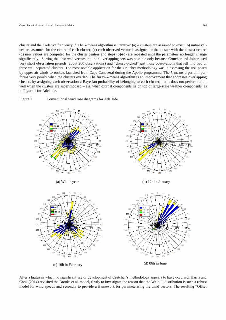
form of the “wind rose” diagram. Example wind roses for Adelaide are shown in Figure 1:

(a) The whole year shows three distinct lobes, attributable to: 30°−50°, land to sea breeze (LS); 130°−170°,

downslope flow (DS); 220°−230°, sea to land breeze (SL); plus less-frequent, but stronger, winds attributable to

large-scale weather systems (LSW).

(b) The sea to land breeze, SL, is dominant in the rose for 12h (1200 local time) in January (midsummer).

(c) The rose for 10h in February shows all three diurnal components are possible at this time of day and season.

(d) The land to sea breeze, LS, is dominant for 06h in June (midwinter).

This form of analysis is purely empirical, not parametric, so is of limited use in wind engineering design.

The alternative to using separate directions and speeds is to consider the horizontal wind vector. Brooks et al. (1946) pa-

rameterised short-duration balloon sonde and surface observations, by resolving the horizontal wind vector into orthogonal

x and y components acting around the mean vector, on the assumptions that both components were normally distributed

and uncorrelated, with means, x and y, and equal standard deviations, x = y. In the Brooks model, contours of equal

joint probability density function (jPDF) appear as concentric circles around the mean vector in the vector plane. Crutcher

(1957) parameterised the wind rose using the jPDF of the bivariate normal distribution in the zonal-meridional plane:

𝑝(𝑊, 𝑆) =

exp(−1

2(1 − 𝜌𝑊𝑆2 )

[(𝑊 − �̅�)2

𝜎𝑊2 − 2𝜌𝑊𝑆

(𝑊 − �̅�)(𝑆 − 𝑆̅)𝜎𝑊𝜎𝑆

+(𝑆 − 𝑆̅)2

𝜎𝑆2 ])

2𝜋𝜎𝑊𝜎𝑆(1 − 𝜌𝑊𝑆2 )0.5

(4)

in terms of the westerly, W, and southerly, S, component, using five parameters: the two means, the two standard devia-

tions and the correlation coefficient. In this model, contours of equal probability density appear as concentric ellipses, cen-

tred on the mean vector, with their principal axes rotated with respect to the W-S axes (Crutcher and Baer 1962). Crutcher

and Joiner (1977a, 1977b) later extended this model to apply in mixed climates, employing the k-means clustering algo-

rithm to sort the observations into k sets of non-overlapping clusters, before computing the five ellipse parameters for each


cluster and their relative frequency, f. The k-means algorithm is iterative: (a) k clusters are assumed to exist; (b) initial val-

ues are assumed for the centre of each cluster; (c) each observed vector is assigned to the cluster with the closest centre;

(d) new values are computed for the cluster centres and steps (b)-(d) are repeated until the parameters no longer change

significantly. Sorting the observed vectors into non-overlapping sets was possible only because Crutcher and Joiner used

very short observation periods (about 200 observations) and “cherry-picked” just those observations that fell into two or

three well-separated clusters. The most notable application for the Crutcher methodology was in assessing the risk posed

by upper air winds to rockets launched from Cape Canaveral during the Apollo programme. The k-means algorithm per-

forms very poorly when the clusters overlap. The fuzzy-k-means algorithm is an improvement that addresses overlapping

clusters by assigning each observation a Bayesian probability of belonging to each cluster, but it does not perform at all

well when the clusters are superimposed – e.g. when diurnal components lie on top of large-scale weather components, as

in Figure 1 for Adelaide.

Figure 1 Conventional wind rose diagrams for Adelaide.

After a hiatus in which no significant use or development of Crutcher’s methodology appears to have occurred, Harris and

Cook (2014) revisited the Brooks et al. model, firstly to investigate the reason that the Weibull distribution is such a robust

model for wind speeds and secondly to provide a framework for parameterising the wind vectors. The resulting “Offset

(a) Whole year (b) 12h in January

(c) 10h in February (d) 06h in June


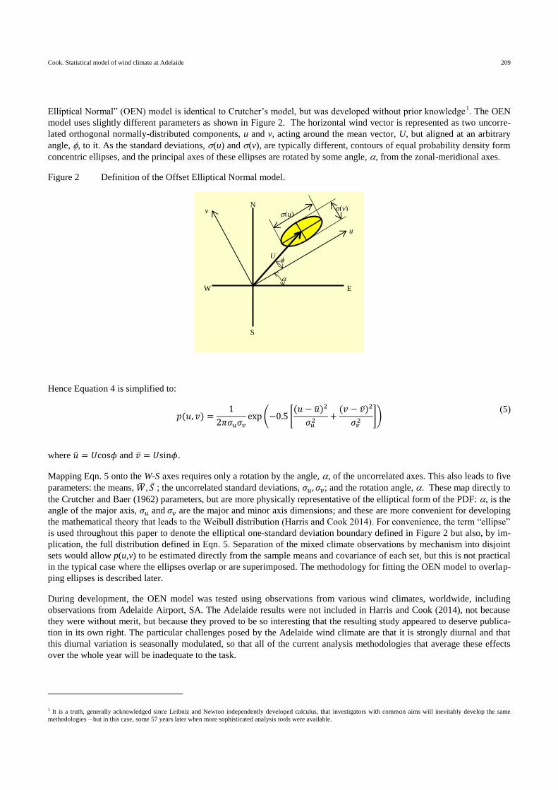
Elliptical Normal” (OEN) model is identical to Crutcher’s model, but was developed without prior knowledge1. The OEN

model uses slightly different parameters as shown in Figure 2. The horizontal wind vector is represented as two uncorre-

lated orthogonal normally-distributed components, u and v, acting around the mean vector, U, but aligned at an arbitrary

angle, , to it. As the standard deviations, (u) and (v), are typically different, contours of equal probability density form

concentric ellipses, and the principal axes of these ellipses are rotated by some angle, , from the zonal-meridional axes.

Figure 2 Definition of the Offset Elliptical Normal model.

Hence Equation 4 is simplified to:

𝑝(𝑢, 𝑣) =

1

2𝜋𝜎𝑢𝜎𝑣exp(−0.5 [

(𝑢 − �̅�)2

𝜎𝑢2

+(𝑣 − �̅�)2

𝜎𝑣2

]) (5)

where �̅� = 𝑈cos𝜙 and �̅� = 𝑈sin𝜙.

Mapping Eqn. 5 onto the W-S axes requires only a rotation by the angle, , of the uncorrelated axes. This also leads to five

parameters: the means, �̅�, 𝑆̅ ; the uncorrelated standard deviations, 𝜎𝑢, 𝜎𝑣; and the rotation angle, . These map directly to

the Crutcher and Baer (1962) parameters, but are more physically representative of the elliptical form of the PDF: , is the

angle of the major axis, 𝜎𝑢 and𝜎𝑣 are the major and minor axis dimensions; and these are more convenient for developing

the mathematical theory that leads to the Weibull distribution (Harris and Cook 2014). For convenience, the term “ellipse”

is used throughout this paper to denote the elliptical one-standard deviation boundary defined in Figure 2 but also, by im-

plication, the full distribution defined in Eqn. 5. Separation of the mixed climate observations by mechanism into disjoint

sets would allow p(u,v) to be estimated directly from the sample means and covariance of each set, but this is not practical

in the typical case where the ellipses overlap or are superimposed. The methodology for fitting the OEN model to overlap-

ping ellipses is described later.

During development, the OEN model was tested using observations from various wind climates, worldwide, including

observations from Adelaide Airport, SA. The Adelaide results were not included in Harris and Cook (2014), not because

they were without merit, but because they proved to be so interesting that the resulting study appeared to deserve publica-

tion in its own right. The particular challenges posed by the Adelaide wind climate are that it is strongly diurnal and that

this diurnal variation is seasonally modulated, so that all of the current analysis methodologies that average these effects

over the whole year will be inadequate to the task.

1 It is a truth, generally acknowledged since Leibniz and Newton independently developed calculus, that investigators with common aims will inevitably develop the same

methodologies – but in this case, some 57 years later when more sophisticated analysis tools were available.

N

E W

S

u

v

U

(u)

(v)


This paper reports the derivation of a parametric statistical model for the wind vectors at Adelaide, SA, from an OEN-

based mixed-climate analysis of the observed wind record with two principal aims in mind. The first aim was to enable

prediction and simulation of the wind climate of Adelaide for use in wind engineering design. The second aim was to elu-

cidate the meteorological mechanisms that drive the seasonal-diurnal variations to improve the current knowledge of this

wind climate. To avoid the issue of confirmation bias: that is finding exactly what is expected and no more; the statistical

model parameters were derived by letting the observations “speak for themselves,” and this forms the bulk of the paper.

The correspondence between the derived model and the known meteorology of the Adelaide region is reviewed in the later

discussion.

Data and methodology

Station data

The 10-minute mean wind speed and wind direction observations for Adelaide Airport, South Australia, were extracted

from the US National Climatic Data Centre (NCDC) archive: comprising the SYNOP (FM-12) and METAR (FM-15) re-

ports from 1973 to 2012 (40 years). These start at 6 hour intervals UTC, progress to 3-hour intervals, but around 70% of

the observations (28 years) form a continuous set at 1 hour intervals, reported on the hour. Provided that the wind climate

is consistent over the 40-year record, the OEN analysis methodology avoids any bias caused by these different intervals.

But, having the largest population, the results at 6 hour intervals are statistically slightly more reliable. However, there is

an issue in that the time of measurement differs from the time of reporting, as recorded in the NCDC database. Jakob

(2010) reveals that the observations at 6- and 3-hour intervals were made in local time: viz. UTC+0930 in winter and

UTC+1030 during daylight saving; but this was not reflected in the NCDC database, which recorded the reports as being

at 6- and 3-hour intervals from 0000 UTC, i.e. on the hour instead of 30 minutes after the hour. As the NCDC database

does not take proper account of either the half-hour offset in local time or the change between standard and daylight sav-

ing, there is an uncertainty spanning about one hour in the time of measurement. From 2006, the NCDC database holds

observations at 30-minute intervals, but it is not clear whether the earlier 30-minute discrepancy still applies. Furthermore,

the 10-minute mean is measured before the reported time – typically, for SYNOP this is the 10-minute period starting 20

minutes before the report. Accordingly, the “local hour-of-day”, H, is defined here as UTC+10000030, representing,

pragmatically, the average of standard and daylight saving time with a 1/2 hour uncertainty. In view of the other observa-

tional approximations: wind speed rounded to integer knot values, wind direction in 10°-wide sectors; the rounding of time

to the nearest hour is not a significant issue. Accordingly, all times in this paper are quoted as local times without minutes,

so noon is H = 12h.

The observations were checked for the bias errors and artefacts described in Cook (2014a) using the automated detection

methodology described in Cook (2014b). The wind speed units were restored from the NCDC archive units (MPH) to the

original units of integer knots. Checks revealed a mild bias between odd and even values in both wind speeds and direc-

tions, but very few artefacts (such as transpositions in the SYNOP codes), all of which were correctable. Recently, the

NCDC SHAF-format database has been replaced by the TD3505-format database which now uses units of m/s in tenths.

Seasonal-diurnal charts

Evaluating the seasonal-diurnal variation for the whole year in terms of month and hour of day requires 288 individual

“wind roses” in the form of Figure 1. In order to visualise these data in a single chart, Cook (2015) devised the colour con-

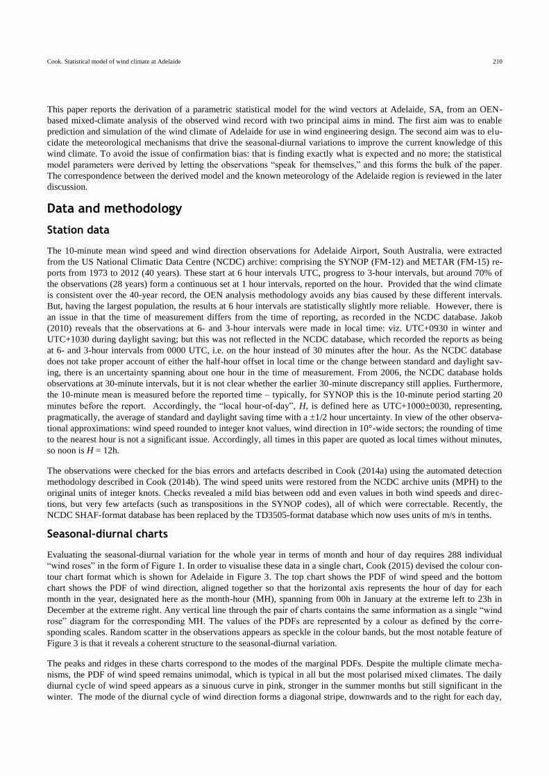
tour chart format which is shown for Adelaide in Figure 3. The top chart shows the PDF of wind speed and the bottom

chart shows the PDF of wind direction, aligned together so that the horizontal axis represents the hour of day for each

month in the year, designated here as the month-hour (MH), spanning from 00h in January at the extreme left to 23h in

December at the extreme right. Any vertical line through the pair of charts contains the same information as a single “wind

rose” diagram for the corresponding MH. The values of the PDFs are represented by a colour as defined by the corre-

sponding scales. Random scatter in the observations appears as speckle in the colour bands, but the most notable feature of

Figure 3 is that it reveals a coherent structure to the seasonal-diurnal variation.

The peaks and ridges in these charts correspond to the modes of the marginal PDFs. Despite the multiple climate mecha-

nisms, the PDF of wind speed remains unimodal, which is typical in all but the most polarised mixed climates. The daily

diurnal cycle of wind speed appears as a sinuous curve in pink, stronger in the summer months but still significant in the

winter. The mode of the diurnal cycle of wind direction forms a diagonal stripe, downwards and to the right for each day,


passing through the peaks corresponding to the modes of the three principal diurnal components (DS, LS, SL), indicating a

sun-wise (anticlockwise in the southern hemisphere) rotation. The annual cycle of large-scale weather systems (LSW) ap-

pears as the wide green band in the background. Note that the LSW component does not appear to show any diurnal varia-

tion, which is expected because the development of these systems has a much longer time scale. The grey “voids” indicate

wind directions that rarely occur.

Figure 3 PDFs of wind speed (top) and direction (bottom) for each Month-Hour over the whole year.

Isolating and assessing calms

“Calms” have two causes: “true calms” comprising about 94%; and “incidental calms”, comprising about 6%. “True

calms” are a distinct, persistent component of the wind climate and will typically occur in consecutive observations where

anemometer and wind vane are both unmoving for some hours. “Incidental calms” occur when there is wind, but V = 0 at

the time of measurement because the mean vector just happens to pass through the origin as the wind conditions change.

So in the hours preceding and succeeding an incidental calm, V > 0 and the wind directions are markedly different. The

contributions from all calms appear in the jPDF as a Dirac delta-function at the origin. The frequency of “incidental calms”

is the value of p(W,S) for the wind vectors interpolated to the origin, and this allows the frequency of “true calms” to be

inferred. As the only significant parameter is the relative frequency of calms, f0, it is convenient to assess and model the

calms and the wind vectors separately, correct f0 for the contribution of “incidental calms”, then to merge the calms back

into the wind model as the final step.

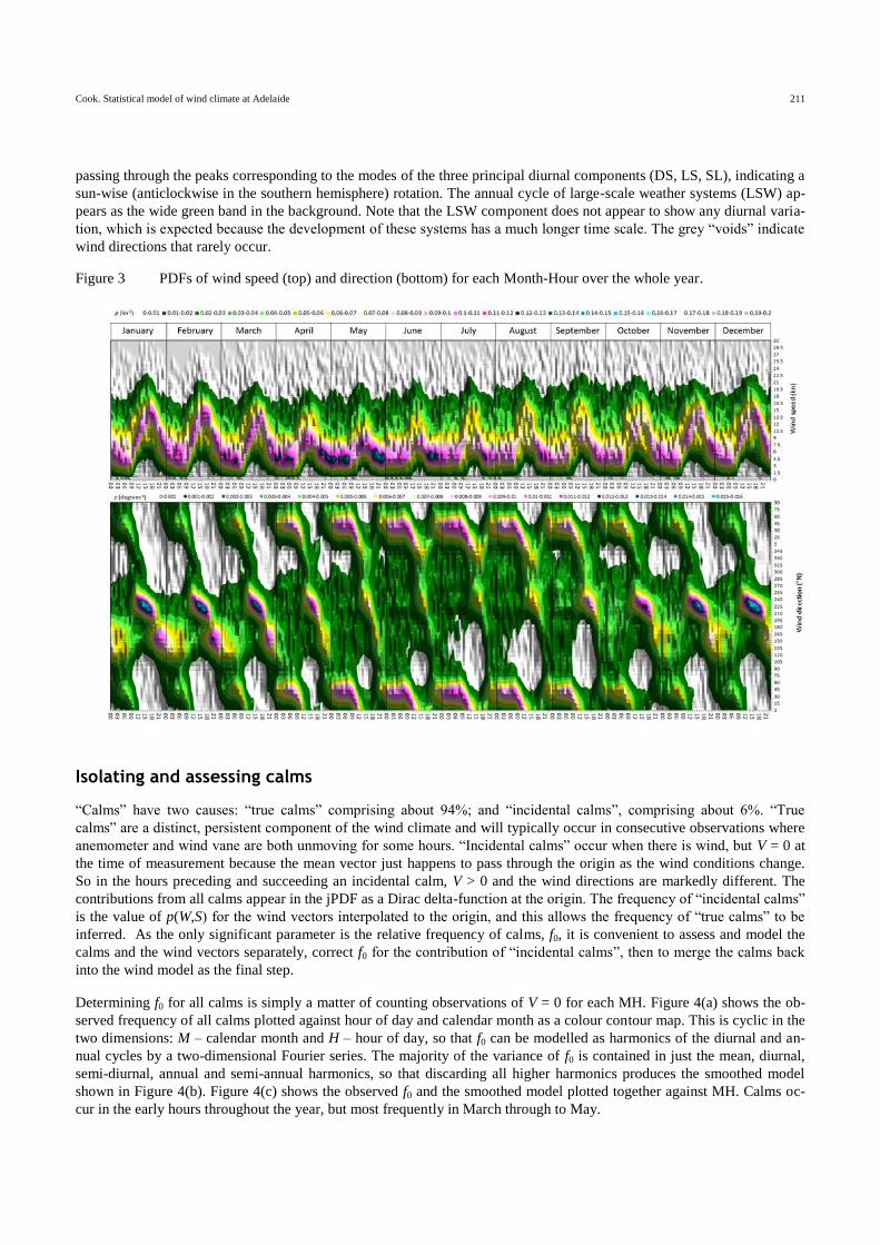
Determining f0 for all calms is simply a matter of counting observations of V = 0 for each MH. Figure 4(a) shows the ob-

served frequency of all calms plotted against hour of day and calendar month as a colour contour map. This is cyclic in the

two dimensions: M – calendar month and H – hour of day, so that f0 can be modelled as harmonics of the diurnal and an-

nual cycles by a two-dimensional Fourier series. The majority of the variance of f0 is contained in just the mean, diurnal,

semi-diurnal, annual and semi-annual harmonics, so that discarding all higher harmonics produces the smoothed model

shown in Figure 4(b). Figure 4(c) shows the observed f0 and the smoothed model plotted together against MH. Calms oc-

cur in the early hours throughout the year, but most frequently in March through to May.


Figure 4 Observed relative frequency, f0, of all calms.

The joint PDF of the wind vectors in the zonal-meridional plane

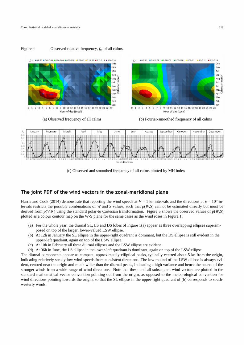
Harris and Cook (2014) demonstrate that reporting the wind speeds at V = 1 kn intervals and the directions at = 10° in-

tervals restricts the possible combinations of W and S values, such that p(W,S) cannot be estimated directly but must be

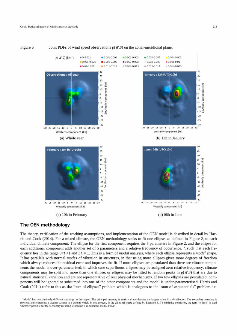
derived from p(V, ) using the standard polar-to Cartesian transformation. Figure 5 shows the observed values of p(W,S)

plotted as a colour contour map on the W-S plane for the same cases as the wind roses in Figure 1:

(a) For the whole year, the diurnal SL, LS and DS lobes of Figure 1(a) appear as three overlapping ellipses superim-

posed on top of the larger, lower-valued LSW ellipse.

(b) At 12h in January the SL ellipse in the upper-right quadrant is dominant, but the DS ellipse is still evident in the

upper-left quadrant, again on top of the LSW ellipse.

(c) At 10h in February all three diurnal ellipses and the LSW ellipse are evident.

(d) At 06h in June, the LS ellipse in the lower-left quadrant is dominant, again on top of the LSW ellipse.

The diurnal components appear as compact, approximately elliptical peaks, typically centred about 5 kn from the origin,

indicating relatively steady low wind speeds from consistent directions. The low mound of the LSW ellipse is always evi-

dent, centred near the origin and much wider than the diurnal peaks, indicating a high variance and hence the source of the

stronger winds from a wide range of wind directions. Note that these and all subsequent wind vectors are plotted in the

standard mathematical vector convention pointing out from the origin, as opposed to the meteorological convention for

wind directions pointing towards the origin, so that the SL ellipse in the upper-right quadrant of (b) corresponds to south-

westerly winds.

(a) Observed frequency of all calms (b) Fourier-smoothed frequency of all calms

(c) Observed and smoothed frequency of all calms plotted by MH index


Figure 5 Joint PDFs of wind speed observations p(W,S) on the zonal-meridional plane.

The OEN methodology

The theory, verification of the working assumptions, and implementation of the OEN model is described in detail by Har-

ris and Cook (2014). For a mixed climate, the OEN methodology seeks to fit one ellipse, as defined in Figure 2, to each

individual climate component. The ellipse for the first component requires the 5 parameters in Figure 2, and the ellipse for

each additional component adds another set of 5 parameters and a relative frequency of occurrence, f, such that each fre-

quency lies in the range 0<f <1 and fi = 1. This is a form of modal analysis, where each ellipse represents a mode2 shape.

It has parallels with normal modes of vibration in structures, in that using more ellipses gives more degrees of freedom

which always reduces the residual error and improves the fit. If more ellipses are postulated than there are climate compo-

nents the model is over-parameterised: in which case superfluous ellipses may be assigned zero relative frequency, climate

components may be split into more than one ellipse, or ellipses may be fitted to random peaks in p(W,S) that are due to

natural statistical variation and are not representative of real physical mechanisms. If too few ellipses are postulated, com-

ponents will be ignored or subsumed into one of the other components and the model is under-parameterised. Harris and

Cook (2014) refer to this as the “sum of ellipses” problem which is analogous to the “sum of exponentials” problem de-

2 “Mode” has two distinctly different meanings in this paper. The principal meaning is statistical and denotes the largest value in a distribution. The secondary meaning is

physical and represents a distinct pattern in a system which, in this context, is the elliptical shape defined by Equation 5. To minimise confusion, the term “ellipse” is used

wherever possible for the secondary meaning, otherwise it is italicised: mode, modal.

(a) Whole year (b) 12h in January

(c) 10h in February (d) 06h in June


scribed by Lanczos (1956) when attempting to separate the individual exponential decay rates of a mixture of radioactive

substances. For brevity, these fits are henceforth referred to as “OENk”, where “k” represents the number of ellipses fitted.

The “wind roses” in Figure 1 and the jPDFs in Figure 5 suggest the k = 4 mechanisms, earlier designated as DS, LS, SL

and LWS. While SL and LS are presumably attributes of a single sea-land breeze mechanism, the fact that either may oc-

cur at a given MH requires that they are modelled separately.

Parameter optimisation – free vs conditional fitting

Optimal values of the OEN parameters may be found by minimising the error between the observed jPDF p(W,S) and the

OEN model. In this case, the root mean square of the error between the observations and the model was used as the error

function and minimisation was implemented in the Microsoft ExcelTM

spreadsheet to exploit its multi-parameter non-linear

optimiser, “Solver”. In this context, “free fitting” denotes optimising the parameters of all ellipses simultaneously, where-

as “conditional fitting” denotes optimising the parameters of each ellipse sequentially while holding the parameters of the

other ellipses constant. Each approach has certain advantages and disadvantages.

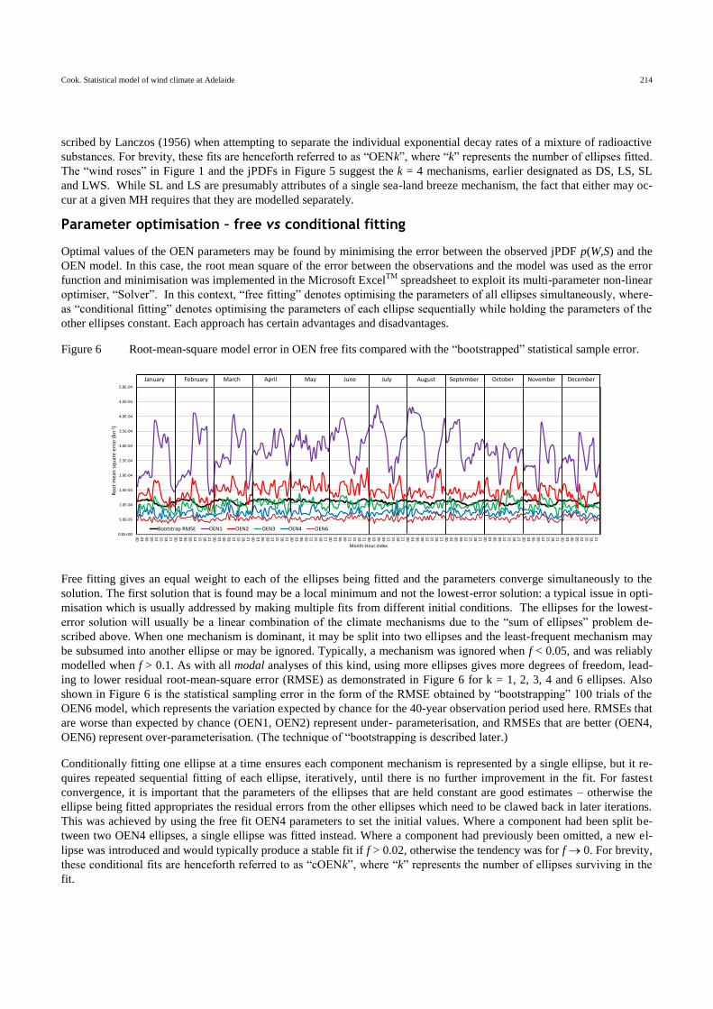
Figure 6 Root-mean-square model error in OEN free fits compared with the “bootstrapped” statistical sample error.

Free fitting gives an equal weight to each of the ellipses being fitted and the parameters converge simultaneously to the

solution. The first solution that is found may be a local minimum and not the lowest-error solution: a typical issue in opti-

misation which is usually addressed by making multiple fits from different initial conditions. The ellipses for the lowest-

error solution will usually be a linear combination of the climate mechanisms due to the “sum of ellipses” problem de-

scribed above. When one mechanism is dominant, it may be split into two ellipses and the least-frequent mechanism may

be subsumed into another ellipse or may be ignored. Typically, a mechanism was ignored when f < 0.05, and was reliably

modelled when f > 0.1. As with all modal analyses of this kind, using more ellipses gives more degrees of freedom, lead-

ing to lower residual root-mean-square error (RMSE) as demonstrated in Figure 6 for k = 1, 2, 3, 4 and 6 ellipses. Also

shown in Figure 6 is the statistical sampling error in the form of the RMSE obtained by “bootstrapping” 100 trials of the

OEN6 model, which represents the variation expected by chance for the 40-year observation period used here. RMSEs that

are worse than expected by chance (OEN1, OEN2) represent under- parameterisation, and RMSEs that are better (OEN4,

OEN6) represent over-parameterisation. (The technique of “bootstrapping is described later.)

Conditionally fitting one ellipse at a time ensures each component mechanism is represented by a single ellipse, but it re-

quires repeated sequential fitting of each ellipse, iteratively, until there is no further improvement in the fit. For fastest

convergence, it is important that the parameters of the ellipses that are held constant are good estimates – otherwise the

ellipse being fitted appropriates the residual errors from the other ellipses which need to be clawed back in later iterations.

This was achieved by using the free fit OEN4 parameters to set the initial values. Where a component had been split be-

tween two OEN4 ellipses, a single ellipse was fitted instead. Where a component had previously been omitted, a new el-

lipse was introduced and would typically produce a stable fit if f > 0.02, otherwise the tendency was for f 0. For brevity,

these conditional fits are henceforth referred to as “cOENk”, where “k” represents the number of ellipses surviving in the

fit.

0.0E+00

5.0E-05

1.0E-04

1.5E-04

2.0E-04

2.5E-04

3.0E-04

3.5E-04

4.0E-04

4.5E-04

5.0E-04

00

03

06

09

12

15

18

21

00

03

06

09

12

15

18

21

00

03

06

09

12

15

18

21

00

03

06

09

12

15

18

21

00

03

06

09

12

15

18

21

00

03

06

09

12

15

18

21

00

03

06

09

12

15

18

21

00

03

06

09

12

15

18

21

00

03

06

09

12

15

18

21

00

03

06

09

12

15

18

21

00

03

06

09

12

15

18

21

00

03

06

09

12

15

18

21

Ro

ot

mea

n s

qu

are

erro

r (k

n-2

)

Month-Hour index

Bootstrap RMSE OEN1 OEN2 OEN3 OEN4 OEN6

January February March April May June July August September October November December


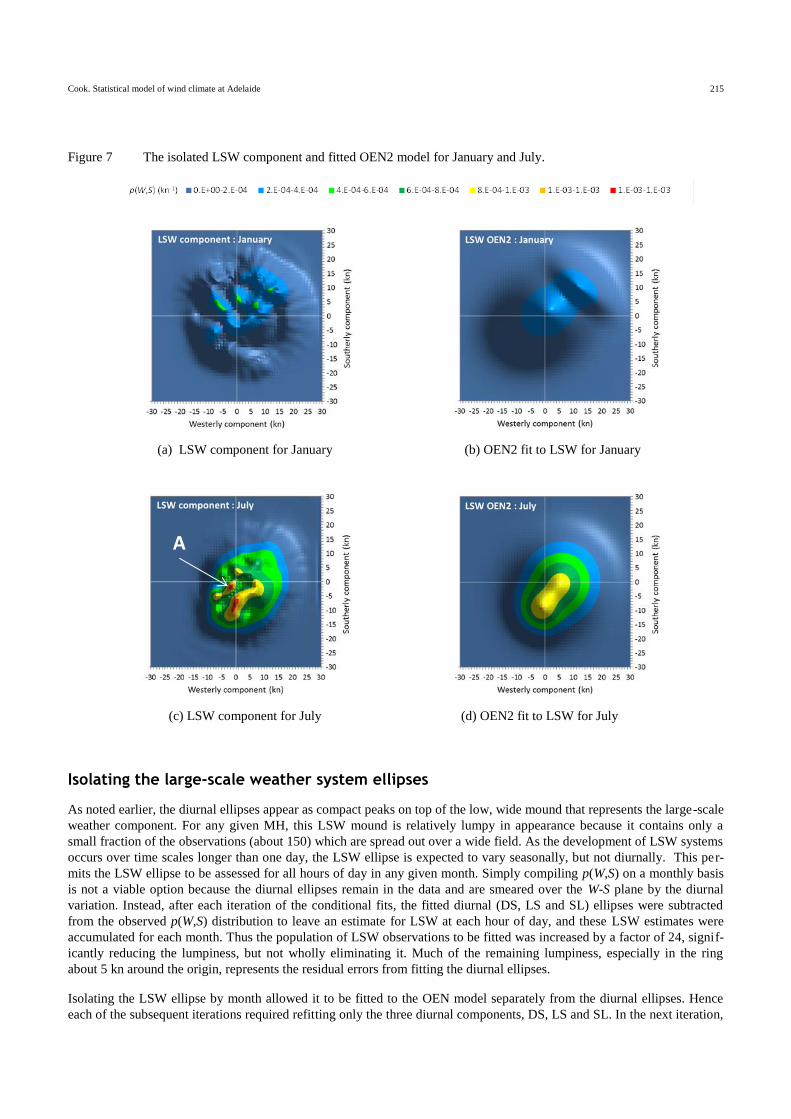
Figure 7 The isolated LSW component and fitted OEN2 model for January and July.

Isolating the large-scale weather system ellipses

As noted earlier, the diurnal ellipses appear as compact peaks on top of the low, wide mound that represents the large-scale

weather component. For any given MH, this LSW mound is relatively lumpy in appearance because it contains only a

small fraction of the observations (about 150) which are spread out over a wide field. As the development of LSW systems

occurs over time scales longer than one day, the LSW ellipse is expected to vary seasonally, but not diurnally. This per-

mits the LSW ellipse to be assessed for all hours of day in any given month. Simply compiling p(W,S) on a monthly basis

is not a viable option because the diurnal ellipses remain in the data and are smeared over the W-S plane by the diurnal

variation. Instead, after each iteration of the conditional fits, the fitted diurnal (DS, LS and SL) ellipses were subtracted

from the observed p(W,S) distribution to leave an estimate for LSW at each hour of day, and these LSW estimates were

accumulated for each month. Thus the population of LSW observations to be fitted was increased by a factor of 24, signif-

icantly reducing the lumpiness, but not wholly eliminating it. Much of the remaining lumpiness, especially in the ring

about 5 kn around the origin, represents the residual errors from fitting the diurnal ellipses.

Isolating the LSW ellipse by month allowed it to be fitted to the OEN model separately from the diurnal ellipses. Hence

each of the subsequent iterations required refitting only the three diurnal components, DS, LS and SL. In the next iteration,

(a) LSW component for January (b) OEN2 fit to LSW for January

(c) LSW component for July (d) OEN2 fit to LSW for July

A


the LSW component was again isolated to give an improved monthly estimate. After the first iteration it was clear that

p(W,S) for the LSW component is bi-modal, with one ellipse (LSW1) dominating in the winter and the other (LSW2) in

the summer. Figure 7 shows the LSW p(W,S) distributions and their fits for January (summer) and July (winter) after the

fourth iteration. The relative frequency of the “winter” component (LSW1) peaks at f = 0.41 in August, falling to f = 0.03

in February; the “summer” component (LSW2) peaks at f = 0.18 in January, falling to f = 0.09 in August.

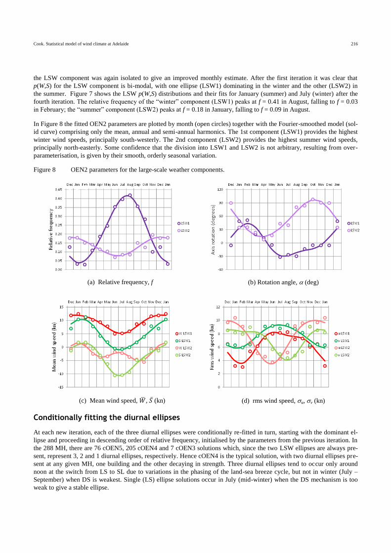
In Figure 8 the fitted OEN2 parameters are plotted by month (open circles) together with the Fourier-smoothed model (sol-

id curve) comprising only the mean, annual and semi-annual harmonics. The 1st component (LSW1) provides the highest

winter wind speeds, principally south-westerly. The 2nd component (LSW2) provides the highest summer wind speeds,

principally north-easterly. Some confidence that the division into LSW1 and LSW2 is not arbitrary, resulting from over-

parameterisation, is given by their smooth, orderly seasonal variation.

Figure 8 OEN2 parameters for the large-scale weather components.

Conditionally fitting the diurnal ellipses

At each new iteration, each of the three diurnal ellipses were conditionally re-fitted in turn, starting with the dominant el-

lipse and proceeding in descending order of relative frequency, initialised by the parameters from the previous iteration. In

the 288 MH, there are 76 cOEN5, 205 cOEN4 and 7 cOEN3 solutions which, since the two LSW ellipses are always pre-

sent, represent 3, 2 and 1 diurnal ellipses, respectively. Hence cOEN4 is the typical solution, with two diurnal ellipses pre-

sent at any given MH, one building and the other decaying in strength. Three diurnal ellipses tend to occur only around

noon at the switch from LS to SL due to variations in the phasing of the land-sea breeze cycle, but not in winter (July –

September) when DS is weakest. Single (LS) ellipse solutions occur in July (mid-winter) when the DS mechanism is too

weak to give a stable ellipse.

(a) Relative frequency, f (b) Rotation angle, (deg)

(d) rms wind speed, u, v (kn) (c) Mean wind speed, �̅�, 𝑆 ̅ (kn)

A


The 5th iteration of the conditional fits is illustrated for the three previous MH examples by Figure 9, Figure 10 and Figure

11. In each figure:

The vector charts for p(W, S) are shown in the top row to allow direct comparison between: (a) the observed vec-

tors; (b) the initial free-fit OEN4 model and (c) the final conditional-fit cOENk model.

The OEN ellipses corresponding to (b) and (c) are shown immediately below the corresponding vector charts as

(d) and (e), respectively.

The conventional meteorological plots in the bottom row show the observations compared with the models for: (f)

the OEN4 marginal wind direction PDF, p() and (g) the OEN4, p(); and (h) cOENk marginal wind speed CDF,

P(V), on Weibull axes.

Figure 9 cOEN analysis for 12h in January.

(a) Observed p(W, S) (b) Free fit OEN4 p(W, S) (c) Conditional fit cOEN5 p(W, S)

(d) Free fit ellipses (e) Conditional fit ellipses

(f) Conditional fit P(V) (g) Free fit p() (h) Conditional fit p()


At H=12h in January, Figure 9, the sea breeze component SL is dominant, but with a significant contribution from DS.

The free fit to OEN4 in (b) has half the RMSE of the conditional fit in (c) to cOEN5 because the SL ellipse is split be-

tween M1 and M4, as confirmed by their relative contributions to the distribution of p() in (g). M4 subsumes the LSW1

component, and M3 merges the LS and LSW2 components. The individual ellipses for DS, LS, SL, LSW1 & LSW2 from

the conditional fit are shown in (e), and the resulting distribution of p() in (h) is not significantly different from (g). The

marginal distribution of wind speed P(V) from the conditional fit in (f) shows that the upper tail of the cOEN5 beyond the

range of the observations is asymptotic to the “summer” LSW2 component, despite its low relative frequency, fLSW2 =

0.18.

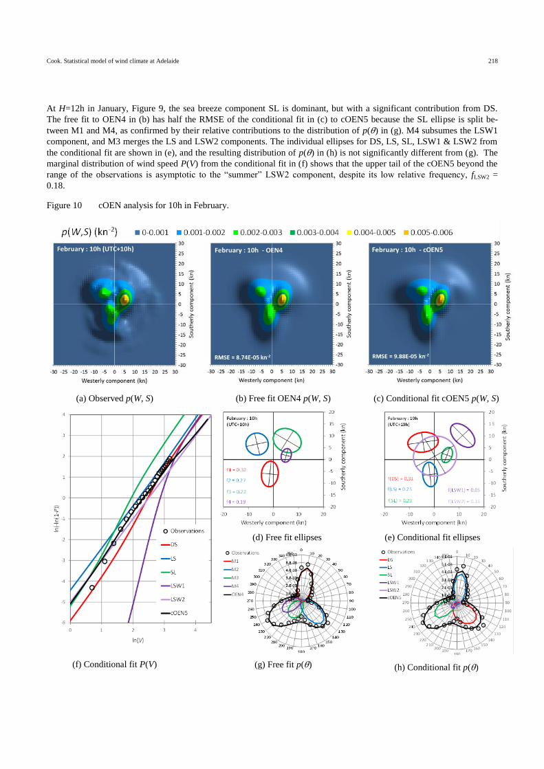
Figure 10 cOEN analysis for 10h in February.





H=10h in February, Figure 10, corresponds to the transition period from “night” to “day” conditions and each of the three

diurnal components is possible. The observed p(W, S) shows waning contributions from DS & LS and a growing contribu-

tion from SL. The free fit to OEN4 in (b) has a slightly lower RMSE than the conditional fit in (c) to cOEN5. However, (d)

shows that the OEN4 fit splits the SL ellipse into two, as confirmed by their relative contributions to the distribution of

p() in (g), and masks out both the LSW components. The individual ellipses for DS, LS, SL, LSW1 & LSW2 from the

conditional fit are shown in (e), and the resulting distribution of p() in (h) is not significantly different from (g). The

marginal distribution of wind speed P(V) from the conditional fit in (f) shows that the upper tail of the cOEN5 beyond the

range of the observations is again asymptotic to the “summer” LSW2 component, despite its low relative frequency, fLSW2

= 0.16.

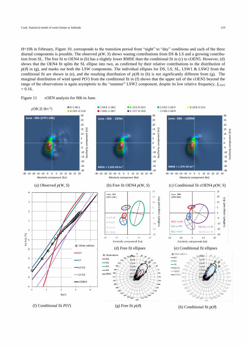
Figure 11 cOEN analysis for 06h in June.





At H=06h in June, Figure 11, the offshore breeze component LS is dominant, with a significant LSW1 component, a very

small contribution from DS and no significant contribution from SL. The free fit to OEN4 in (b) has 3/4 of the RMSE of

the conditional fit in (c) to cOEN4 because the dominant LS ellipse is split between M1 and M2, as confirmed by their

relative contributions to the distribution of p() in (g). The M3 ellipse is elongated because it includes some of LSW2 with

the LSW1 component. The individual ellipses for DS, LS, SL, LSW1 & LSW2 from the conditional fit are shown in (e),

and the resulting distribution of p() in (h) is not significantly different from (g). The marginal distribution of wind speed

P(V) from the conditional fit in (f) shows that the upper tail of the cOEN5 beyond the range of the observations is asymp-

totic to the significant “winter” LSW1 component.

In general, only subtle differences exist between (b) the initial free and (c) the final conditional models of p(W, S). Both

are smoothed versions of the observations (a), but the residual RMSEs for the free fits are consistently smaller than for the

conditional fits. Assigning a single ellipse to each component constrains the contours in (c) to be elliptical, whereas (b)

can allow a linear combination of ellipses to mimic deviations from the elliptical form. Consequently, the smallest RSME

is obtained by splitting a dominant ellipse and ignoring the weakest component. This is apparent in (f), for p(), where the

SL lobe in Figure 10 and the LS lobe in Figure 11 are each formed by the sum of two ellipses. While the OEN models for

p() in (f) and (g) are very similar, the corresponding ellipses in (d) and (e) are very different. In all three figures the

OEN4 model (d) omits the contributions of LSW1 so that the size and position of the other ellipses (except the most domi-

nant ellipse) differ from (e) in compensation. This reflects the comments of Harris and Cook (2014) on the “sum of ellip-

ses” problem, that the division between ellipses can be quite arbitrary and the resulting statistical model will still produce

good values of p(W, S), P(V) and p(). However, to gain any useful insights into the climate mechanisms, each mechanism

must be represented by an individual ellipse, and this is the principal purpose of the OEN methodology – viz. to derive a

phenomenological black-box model of the Adelaide wind climate rather than just to replicate the observations.

Estimating the OEN errors using Bootstrapping

The errors associated with the fitted cOENk models have two main components: the model error – how well the bivariate

normal model represents each component; and the statistical sampling error – how well the particular finite observation

period represents the long-term climate. “Bootstrapping” (Efron and Tibshirani 1993; Naess and Clausen 2001; Cook

2004) is a Monte-Carlo sampling technique for estimating the sampling error inherent in analysing a finite sample taken

from a continuous process. In this context, sets of synthetic observations with the same population as the real observations

are generated by randomly sampling the fitted distributions, then rounding to 1-knot and 10° intervals to mimic the obser-

vation protocol, so that each set is equivalent to the observations but is randomly different. Repeating many trials of this

procedure enables the distribution of the sampling errors to be compiled. In essence, the fitted parameters are used to as-

sess their own statistical confidence – hence “lifting oneself up by one’s own bootstraps”. It requires 104 bootstrap trials to

achieve an accuracy of 1%, but this would take about 48 days to generate, and about 9 years to fit for all 288 MH using a

2.6GHz Intel i5 processor with 4 cores. The pragmatic compromise adopted here was to generate only 100 trials (accuracy

about 10%) for all 288 MH, but to fit LSW parameters to only the three example months and to fit diurnal parameters to

only the three previous example MHs.

In Figure 12 the residual RMSE for the 5th

cOENk iteration is seen to be a reasonable match to the bootstrapped statistical

RMSE for the 40-year observation period, and suggests that the conditional fit provides an optimal model for the long-

term seasonal-diurnal variation. On the other hand, the residual RSME for the initial OEN4 fit is lower than the expected

RMSE and indicates that the free-fit better replicates the observed wind vectors. This is a subtle difference which hinges

on the distinction between “modelling” and “replication”.

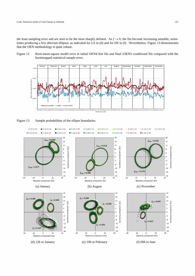
Conditionally fitting the parameters to each of the 100 bootstrap trials allows the mean bias and standard deviation of each

parameter to be assessed to about 10% accuracy. The random variation between trials is visualised in Figure 13 by super-

imposing the fitted ellipses for all 100 trials, such that the colour scale shows the probability of the location of each ellipse

boundary to a resolution of 0.2 kn. In (a) – (c) the trials for the non-diurnal LSW parameters were fitted using OEN2 for

the months shown: (a) January – mid-summer, with LSW2 dominant; (b) August: mid-winter, with LSW1 dominant; and

(c) November – spring, with both LSW components approximately equal. In (d) – (f) the diurnal components were condi-

tionally fitted using five iterations but, typically, convergence was achieved after only 2 iterations. The standard deviation

of the sampling error for each ellipse is inversely proportional to (𝑓𝑘𝑁𝑀𝐻)0.5, where NMH is the population of observations

for the given MH and fk is the relative frequency of the kth ellipse component – so the sampling error increases as the rela-

tive frequency decreases. Accordingly, the most dominant ellipses, SL in (d) ( fSL = 0.495) and LS in (f) ( fLS = 0.527) have


the least sampling error and are seen to be the most sharply defined. As f 0, the fits become increasing unstable, some-

times producing a few aberrant ellipses, as indicated for LS in (d) and for DS in (f). Nevertheless, Figure 13 demonstrates

that the OEN methodology is quite robust.

Figure 12 Root-mean-square model error in initial OEN4 free fits and final cOEN5 conditional fits compared with the

bootstrapped statistical sample error.

Figure 13 Sample probabilities of the ellipse boundaries.

0

0.00005

0.0001

0.00015

0.0002

00

03

06

09

12

15

18

21

00

03

06

09

12

15

18

21

00

03

06

09

12

15

18

21

00

03

06

09

12

15

18

21

00

03

06

09

12

15

18

21

00

03

06

09

12

15

18

21

00

03

06

09

12

15

18

21

00

03

06

09

12

15

18

21

00

03

06

09

12

15

18

21

00

03

06

09

12

15

18

21

00

03

06

09

12

15

18

21

00

03

06

09

12

15

18

21

Ro

ot

mea

n s

qu

are

erro

r (k

n-2

)

Month-Hour index

Bootstrap RMSE OEN4 LSW.cOEN5

January February March April May June July August September October November December

(a) January (b) August (c) November

(d) 12h in January (e) 10h in February (f) 06h in June


The OEN model

Relative frequencies

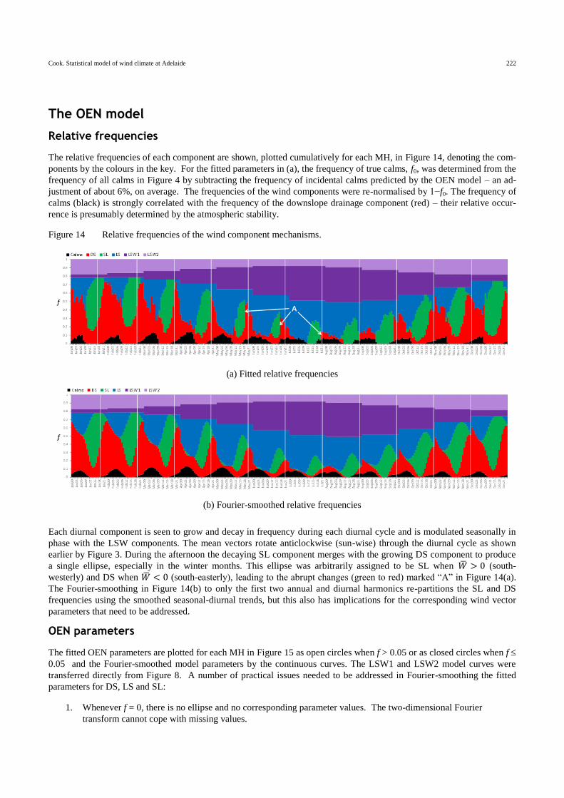
The relative frequencies of each component are shown, plotted cumulatively for each MH, in Figure 14, denoting the com-

ponents by the colours in the key. For the fitted parameters in (a), the frequency of true calms, f0, was determined from the

frequency of all calms in Figure 4 by subtracting the frequency of incidental calms predicted by the OEN model – an ad-

justment of about 6%, on average. The frequencies of the wind components were re-normalised by 1−f0. The frequency of

calms (black) is strongly correlated with the frequency of the downslope drainage component (red) – their relative occur-

rence is presumably determined by the atmospheric stability.

Figure 14 Relative frequencies of the wind component mechanisms.

Each diurnal component is seen to grow and decay in frequency during each diurnal cycle and is modulated seasonally in

phase with the LSW components. The mean vectors rotate anticlockwise (sun-wise) through the diurnal cycle as shown

earlier by Figure 3. During the afternoon the decaying SL component merges with the growing DS component to produce

a single ellipse, especially in the winter months. This ellipse was arbitrarily assigned to be SL when �̅� > 0 (south-

westerly) and DS when �̅� < 0 (south-easterly), leading to the abrupt changes (green to red) marked “A” in Figure 14(a).

The Fourier-smoothing in Figure 14(b) to only the first two annual and diurnal harmonics re-partitions the SL and DS

frequencies using the smoothed seasonal-diurnal trends, but this also has implications for the corresponding wind vector

parameters that need to be addressed.

OEN parameters

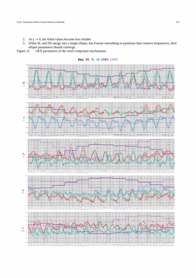
The fitted OEN parameters are plotted for each MH in Figure 15 as open circles when f > 0.05 or as closed circles when f

0.05 and the Fourier-smoothed model parameters by the continuous curves. The LSW1 and LSW2 model curves were

transferred directly from Figure 8. A number of practical issues needed to be addressed in Fourier-smoothing the fitted

parameters for DS, LS and SL:

1. Whenever f = 0, there is no ellipse and no corresponding parameter values. The two-dimensional Fourier

transform cannot cope with missing values.

(a) Fitted relative frequencies

(b) Fourier-smoothed relative frequencies


2. As f 0, the fitted values become less reliable.

3. When SL and DS merge into a single ellipse, but Fourier-smoothing re-partitions their relative frequencies, their

ellipse parameters should converge.

Figure 15 OEN parameters of the wind component mechanisms.

Key: DS SL LS LSW1 LSW2


These issues were resolved by the following steps:

(a) Arbitrary, but realistic initial values were assigned to the OEN parameters when f = 0.

(b) Fourier-smoothing was performed using these initial values.

(c) Wherever f was less than a minimum threshold value of f = 0.05, the fitted values were replaced by the model

values from step (b).

(d) To ensure that DS and SL had convergent parameters when re-partitioned from a single merged ellipse, the fitted

value of DS was replaced by the model value of SL when fDS<0.05 and vice-versa when fSL<0.05.

(e) Steps (b) to (d) were repeated iteratively until there was no further change to the model parameters at the third

significant figure. These iterations were implemented automatically in the Excel spreadsheet through the use of

“circular references”. Around 100 iterations are needed to achieve convergence.

The mean speed parameters, �̅� and 𝑆̅, are a better match to the smooth model than the rms parameters, 𝜎𝑢 and 𝜎𝑣, the lat-

ter tending to have high-valued outliers as f0. The outliers for the axis rotation angle, , tend to occur when 𝜎𝑢 ≈ 𝜎𝑣,

when the ellipse is nearly circular and the angle becomes indeterminate. The diurnal cycles of �̅�and 𝑆̅ show a characteris-

tic half-wave rectified sinusoid shape which mirrors the shape of the insolation cycle (Cook 2012) but lags it by 1 to 2

hours. The diurnal cycles of 𝜎𝑢 and 𝜎𝑣 are similar in form, but less well organised.

Seasonal-diurnal charts

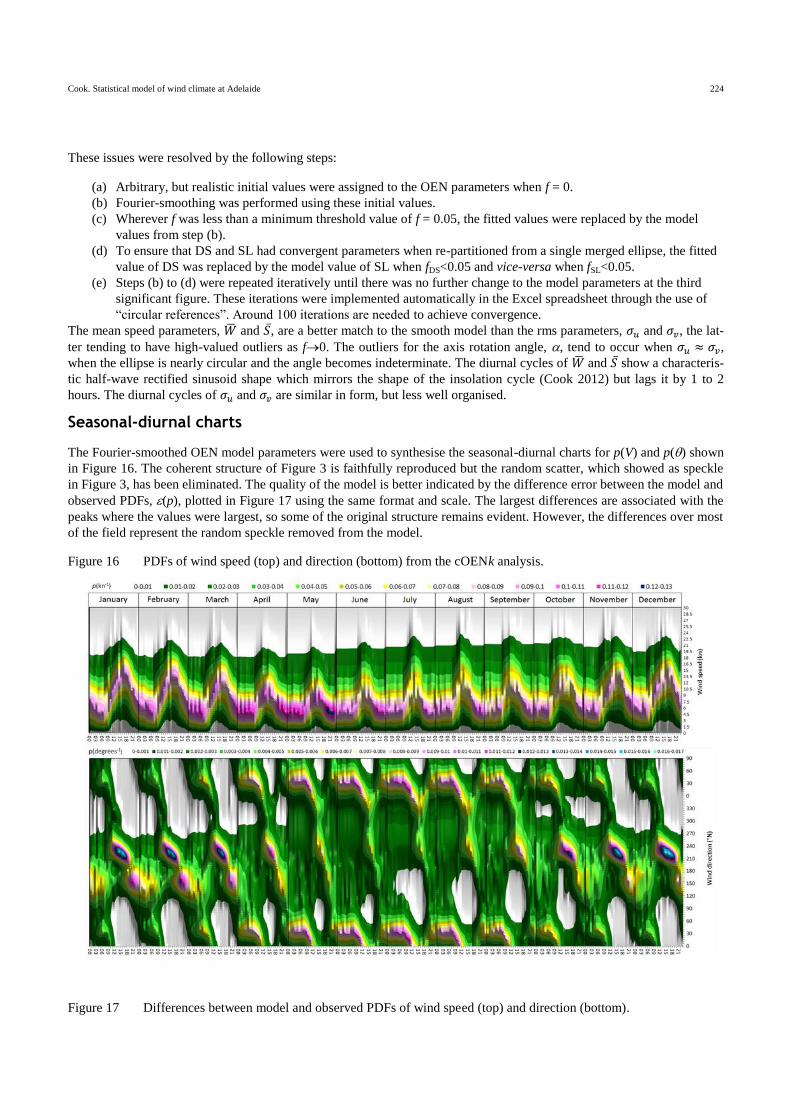
The Fourier-smoothed OEN model parameters were used to synthesise the seasonal-diurnal charts for p(V) and p() shown

in Figure 16. The coherent structure of Figure 3 is faithfully reproduced but the random scatter, which showed as speckle

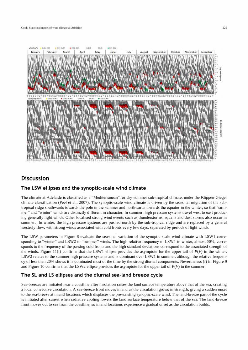
in Figure 3, has been eliminated. The quality of the model is better indicated by the difference error between the model and

observed PDFs, (p), plotted in Figure 17 using the same format and scale. The largest differences are associated with the

peaks where the values were largest, so some of the original structure remains evident. However, the differences over most

of the field represent the random speckle removed from the model.

Figure 16 PDFs of wind speed (top) and direction (bottom) from the cOENk analysis.

Figure 17 Differences between model and observed PDFs of wind speed (top) and direction (bottom).


Discussion

The LSW ellipses and the synoptic-scale wind climate

The climate at Adelaide is classified as a “Mediterranean”, or dry-summer sub-tropical climate, under the Köppen-Gieger

climate classification (Peel et al., 2007). The synoptic-scale wind climate is driven by the seasonal migration of the sub-

tropical ridge southwards towards the pole in the summer and northwards towards the equator in the winter, so that “sum-

mer” and “winter” winds are distinctly different in character. In summer, high pressure systems travel west to east produc-

ing generally light winds. Other localised strong wind events such as thunderstorms, squalls and dust storms also occur in

summer. In winter, the high pressure systems are pushed north by the sub-tropical ridge and are replaced by a general

westerly flow, with strong winds associated with cold fronts every few days, separated by periods of light winds.

The LSW parameters in Figure 8 evaluate the seasonal variation of the synoptic scale wind climate with LSW1 corre-

sponding to “winter” and LSW2 to “summer” winds. The high relative frequency of LSW1 in winter, almost 50%, corre-

sponds to the frequency of the passing cold fronts and the high standard deviations correspond to the associated strength of

the winds. Figure 11(f) confirms that the LSW1 ellipse provides the asymptote for the upper tail of P(V) in the winter.

LSW2 relates to the summer high pressure systems and is dominant over LSW1 in summer, although the relative frequen-

cy of less than 20% shows it is dominated most of the time by the strong diurnal components. Nevertheless (f) in Figure 9

and Figure 10 confirms that the LSW2 ellipse provides the asymptote for the upper tail of P(V) in the summer.

The SL and LS ellipses and the diurnal sea-land breeze cycle

Sea-breezes are initiated near a coastline after insolation raises the land surface temperature above that of the sea, creating

a local convective circulation. A sea-breeze front moves inland as the circulation grows in strength, giving a sudden onset

to the sea-breeze at inland locations which displaces the pre-existing synoptic-scale wind. The land-breeze part of the cycle

is initiated after sunset when radiative cooling lowers the land surface temperature below that of the sea. The land-breeze

front moves out to sea from the coastline, so inland locations experience a gradual onset as the circulation builds.


Theory (Haurwitz 1947, Staley 1957, 1989) predicts that the wind direction should be normal to the coastline at onset of

the sea- or land-breeze then gradually rotate sun-wise, driven by the Coriolis force, until parallel with the coast. Simpson

(1996) concludes that Coriolis force is not always the dominant term in the equations of motion. There are many published

events showing simple on-shore/off-shore cycles without any significant rotation, or with reversed rotation. An example

of this is the study of sea-breezes around Sardinia in the Mediterranean by Furberg et al. (2002), in which the mean hourly

hodographs for 12 observation stations around the coast are nearly closed and aligned on-shore/off-shore to the local coast-

line, any weak rotation being sometimes sun-wise, sometimes reversed and sometimes both directions in a figure of eight

form. The recent numerical model by Moisseeva and Steyn (2012) using an idealised representation of Sardinia reproduces

some of these effects. The consensus (Kusada and Alpert 1983, Steyn and Kallos 1992, Furberg et al. 2002, Moisseeva and

Steyn 2012) is that the rotation is controlled by a delicate balance between Coriolis force, surface and synoptic pressure

gradients, topography and advection effects.

However, these theories apply to a straight coastline. Dexter (1958) showed that at Halifax, Nova Scotia, where the local

harbour coastline lies at 70° to the Atlantic coastline, the sea-breeze is normal to the local coastline at onset, but turns

normal to the Atlantic coastline by late afternoon. Although this is a sun-wise rotation compatible with the Coriolis force,

the resulting hodograph was well represented by the sum of two elliptical hodographs, one aligned to the local coastline

and the other to the Atlantic coastline, which he suggested was due to two separate but sequential sea-breezes at different

scales. Following this theme, Physick and Byron-Scott (1977) investigated the development of sea-breezes at various loca-

tions around Gulf St Vincent, including Adelaide on the west-facing coast and, significantly, Stansbury on the opposite

east-facing coast. As the sea-breeze develops, the wind direction at Adelaide turns anticlockwise from westerly onshore to

southerly alongshore, but the wind direction at Stansbury turns clockwise from easterly onshore to southerly alongshore.

Physick and Byron-Scott conclude that two sea-breeze mechanisms exist: the initial “Gulf” sea-breeze that is locally on-

shore and is driven by the Gulfland temperature difference; and the later “continental” sea-breeze that is southerly and is

driven by the Southern OceanAustralian continent temperature difference. The Coriolis force assists the rotation at Ade-

laide and resists the rotation at Stansbury, but is overcome by the “continental” sea breeze that is strong enough for the

sea-breeze front to penetrate 300 km inland on occasion (Clarke 1955).

The primary driver of the sea-land breeze cycle is the temperature difference between land and sea, while the effects that

may cause rotation of the wind direction are secondary modifiers. It seems likely that the rotation of the sea-breeze found

in some of the previous studies may be due this primary effect acting on multiple coastlines. This possibility deserves in-

vestigation by review of the previous studies.

At Adelaide, the SL ellipse represents the sea-breezes which start westerly just before noon and rotate sun-wise to souther-

ly by late afternoon in a continuous fashion (Figure 3 and Figure 16), so that the average direction is southwesterly (see

Figure 19(b), later). As the sea-breeze fades in the early evening, the wind direction continues to rotate until it coincides

with the direction of the downslope winds. The land-breeze starts north-easterly in the late evening and tends to maintain

this direction until dawn, before also rotating sun-wise to northerly. Onset is delayed in the summer months by the strong

downslope winds, as the land-breeze speeds are generally weaker than SL and DS speeds. While the relative frequencies of

the SL ellipses in Figure 14 show the expected diurnal variation for sea-breezes, the LS ellipses are only totally excluded

during daylight from November to March when SL is most dominant. The LS ellipses are evident at all hours of day in the

period April through October, so must represent more than just the expected nocturnal land-breezes. Tepper and Watson

(1990) show that, at night, the typical surface wind is blocked and forced to run northeasterly, parallel to the Adelaide

Hills – but this does not account for the persistence of LS during the day. It is possible that the land remains sufficiently

colder than the sea to permit an existing land-breeze to continue as a gentle NE drift on days where dense cloud cover re-

duces sensible surface heating

The previous studies, cited earlier, all addressed individual or averages of selected “sea-breeze days”, so were able to ob-

serve the sudden onset. Physically, sea- and land-breezes are mutually exclusive so their relative frequencies at a given

MH are disjoint and the appearance of both SL and LS ellipses at the same MH is purely statistical. The onset of the sea-

breeze in the statistical model appears to be gradual only because the time of onset is variable from day to day: around 3

hours for the onset of SL (Figure 14). Both the sea- and land-breeze parts of the cycle are affected by the pre-existing syn-

optic winds: at low synoptic wind speeds the direction of the gradient wind may advance onset if offshore or delay onset if

onshore, i.e. acting with or against the off-shore flow at the top of the sea-breeze circulation. At high onshore wind speeds

the circulation cell may not form at all. In the UK, it is generally accepted that sea-breezes are unlikely to establish when

the pre-existing onshore gradient wind speed exceeds about 16 kn (Brittain 1966). Studies specific to Adelaide collated by


Ferrière (1994), indicate that the strongest SW sea breezes occur when the gradient wind is SE and is greater than 18 kt.

The OEN model implicitly assumes that the relative probabilities of each ellipse are independent of the pre-existing wind

speed. Figure 9(f) illustrates that where SL is dominant, the observations do not fit the OEN model at low wind speeds,

but instead follow the SL component, indicating that the relative frequency for SL is speed-dependent and approaches

100% at these low speeds.

The daily cycle of insolation that drives the sea-land breezes has the form of a half-wave rectified sine; that is, a curve ris-

ing from zero at dawn to a maximum at noon and falling to zero at dusk as the positive lobe of a sine. Through the night

the insolation is zero so the insolation curve is flat. Radiative losses are constant throughout the day and night, so that the

net heating of the surface is positive during the day and negative at night. Dai and Deser (1999) describe this process and

its consequences as follows:

“Solar heating in the atmosphere, combined with other regional forcings, generates internal gravity waves in the at-

mosphere at periods of integral fractions of a solar day, especially at the diurnal and semidiurnal periods. These

waves cause regular oscillations in atmospheric pressure, temperature, and wind fields which are often referred to as

atmospheric tides.”

Therefore it is not a surprise that the seasonal-diurnal variation of �̅� and 𝑆̅ in Figure 15 exhibits exactly the same form,

modulated by season, and is also well represented by the first two diurnal harmonics. For �̅�, SL and LS remain locked in

phase, but lagging the insolation curve by about three hours. For LS, 𝑆̅ indicates a mean northerly drift, stronger in the

winter, this averages with �̅�to north-easterly (see Figure 19(b), later). The variation of the rms components in Figure 15

is similar, but less well organised.

The DS ellipses and the downslope “gully” winds

The seasonal-diurnal variation of sea-land breeze cycle is made more complex by interaction with the downslope winds.

At many other locations, a coastal plain is backed by topography that lies parallel to the coast, so that nocturnal downslope

winds and land-breezes have a common direction and augment each other. At Adelaide the scarp of the Adelaide Hills

faces northwest, leading to the strong, but shallow, southeasterly downslope drainage winds known locally as “gully”

winds. Sha et al. (1996) describe gully winds as a nocturnal occurrence with a sudden onset, variable in strength but not

direction, usually occurring behind a steep leeward-facing ramp when an inversion exists just above hill-top level. They

report a number of contradictory and complementary mechanisms proposed by various authors – including that the after-

noon sea-breeze is unable to climb over the Mt Lofty ranges and is trapped, building to a sufficient height to cascade down

the northwest-facing slope as a shallow gravity current – but state that this explanation is insufficient to account for

strongest events. They note that the effect on the coastal plain is similar to a hydraulic jump or to a breaking wave and

conclude that: “The characteristics of the Adelaide gully wind are an aspect for further study”.

Grace and Holton (1990) review the hydraulic jump theory and describe how the SE surface wind of the shallow flow

across the plain accelerates just before the jump, then suddenly reverses direction to NW in the weak rotor that forms after

the jump, and they show examples of this behaviour in simultaneous observations at locations around Adelaide. Sudden

onset of strong winds occurs at locations on the coastal plain as the flow strengthens and the jump migrates towards the

coast. They also note that the moderate wind speeds in the original SE direction have been observed downwind of the rotor

and that the sudden pressure rise associated with the jump is unlikely to be detected as it is typically less than 0.5hPa. They

conclude that none of the other proposed mechanisms, e.g. cold ponding, accounts fully for these observations.

The DS ellipses are consistent with the southeasterly gully winds. As with SL, onset of DS appears gradual in the statisti-

cal model only because the time of onset is variable. The predicted reversed flow in the rotor is too weak to be distin-

guished from the random noise (Figure 17). The OEN analysis confirms that DS is essentially a nocturnal summer phe-

nomenon and Figure 3 and Figure 16 show that southeasterly winds are rare in the midwinter months. However, the persis-

tence of DS through summer afternoons, albeit at the low frequency shown in Figure 14, and the corresponding excursions

to higher mean wind speeds in the hodograph, Figure 18 (described later), hints of an additional causal mechanism. Evalu-

ation of the seasonal-diurnal variation of the DS parameters in Figure 14 and Figure 15 appears to be the first contribution

on gully winds since Sha et al. (1996) called for further study.


Overview of results

This paper reports the statistical analysis and modelling of the seasonal-diurnal variations of wind vectors at Adelaide. The

cOENk methodology quantifies the wind vectors using k bivariate normal distributions, or “ellipses”, in the zonal-

meridional plane, where k is the number of individual climate mechanisms represented. Parameters were fitted by condi-

tionally optimising the distribution parameters for each mechanism at each month-hour. The synoptic-scale mechanisms

were isolated by subtracting the diurnal ellipses from the observed distribution at each MH, then summing the resulting 24

distributions to obtain the synoptic-scale distributions. This is an improvement to the recent OEN method of Cook and

Harris (2014) because it prevents the splitting of the k mechanisms into arbitrary linear combinations which, while still

providing a good statistical model for simulation and prediction purposes, obfuscates interpretation of the physical mecha-

nisms. The cOENk methodology is superior to the previous k-means clustering methodology used by Crutcher and his as-

sociates because it copes well with the diurnal components being superimposed on the synoptic-scale components: made

possible because of advances in computing power and optimisation techniques which were unavailable to Crutcher at the

time.

As the methods used in this work are novel, their accuracy and robustness had to be assessed internally. The overall fit of

the model to the observations was quantified by the RMSE – but this does not indicate how the errors are distributed. Alt-

hough graphical comparisons between the observed and model jPDFs show an excellent match, this is only qualitative.

Bootstrapping techniques demonstrated the robustness of the cOEN methodology by assessing its ability to recover the

model parameters from simulated observations randomly sampled from them. The quality of the final model was demon-

strated by showing that the residual errors mostly comprised random scatter, with only a small indication of the organised

seasonal-diurnal structure.

The seasonal-diurnal variation of the wind climate at Adelaide was assessed by a “blind” implementation of the OEN

method – that is, without direct reference to the known meteorology of the area – avoiding any confirmation bias and al-

lowing the data “to speak for themselves”. This revealed a strongly organised structure to the seasonal-diurnal variations

which is well represented in the cOENk model by using only the mean, annual, semi-annual, diurnal and semi-diurnal

harmonics. The principal components were shown to be two synoptic-scale components, designated LSW1 or “winter”

and LSW2 “summer”, and three diurnal components: a downslope drainage flow DS, a land-to-sea flow LS and a sea-to-

land flow SL. These results were compared with the known meteorology of Gulf St Vincent and Adelaide earlier. The el-

ements that make Adelaide particularly interesting over other coastal locations are the local-continental two-coast effect on

the sea-land breeze cycle, the additional gully wind mechanism that acts at right-angles to this, the turning of shallow

flows to run parallel to the Adelaide Hills and the interaction of the diurnal components with the “summer” and “winter”

synoptic-scale winds that vary with the seasonal migration of the sub-tropical ridge.

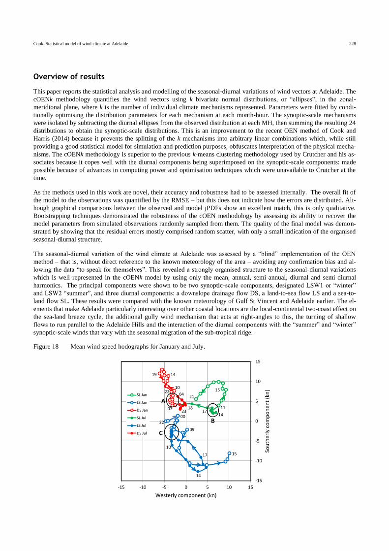
Figure 18 Mean wind speed hodographs for January and July.

-15

-10

-5

0

5

10

15

-15 -10 -5 0 5 10 15

Sou

ther

ly c

om

po

nen

t (k

n)

Westerly component (kn)

SL Jan

LS Jan

DS Jan

SL Jul

LS Jul

DS Jul

15

00

22

17

14

10

21

11

15

1417

18

A

B09

04

23

1419

10

07

22

C


An overview of the complexity of the diurnal components is given by the hodographs for the mean speed parameters, �̅�

and 𝑆̅, shown in Figure 18 for the months of January (midsummer) and July (midwinter) for each of the diurnal ellipses.

The time of day is indicated next to some of the values and the progression of time is indicated by the arrowheads. The

DS ellipse is essentially a summer nocturnal phenomenon, remaining in the zone labelled “A” whilst dominant in January.

The daytime excursions of DS to higher mean wind speeds in January remain in the same SE direction and hint of a

different cause. The SL ellipse in January forms an open loop from 11h to 21h, and the kink at 15h can be interpreted as

the change from “local” to “continental” sea-breeze. The weaker winter SL ellipse in July remains in the zone “B” from

SW through most of the afternoon before rotating to south at dusk. The LS ellipse is essentially a winter nocturnal

phenomenon, remaining from NE in the zone “C” whilst dominant in July. In January the LS ellipse forms an open loop in

two stages: from 22h to 09h rotating from NE to N, then from 09h to 15h rotating from N to NW, which again can be

attributed to “local” and “continental” land-breezes. The daytime excursions of LS in July through north towards

northwesterlies mirrors the second stage of the January loop. The evening return loop of LS in the winter is revealed in the

seasonal-diurnal charts, Figure 3 and Figure 16, as the V-shaped links (yellow-pink) connecting the LS peaks only in the

winter months. These links indicate an alternative path to the diagonal stripes of the anticlockwise rotation, whereby the

LS component returns clockwise omitting the sea-breeze half of the cycle.

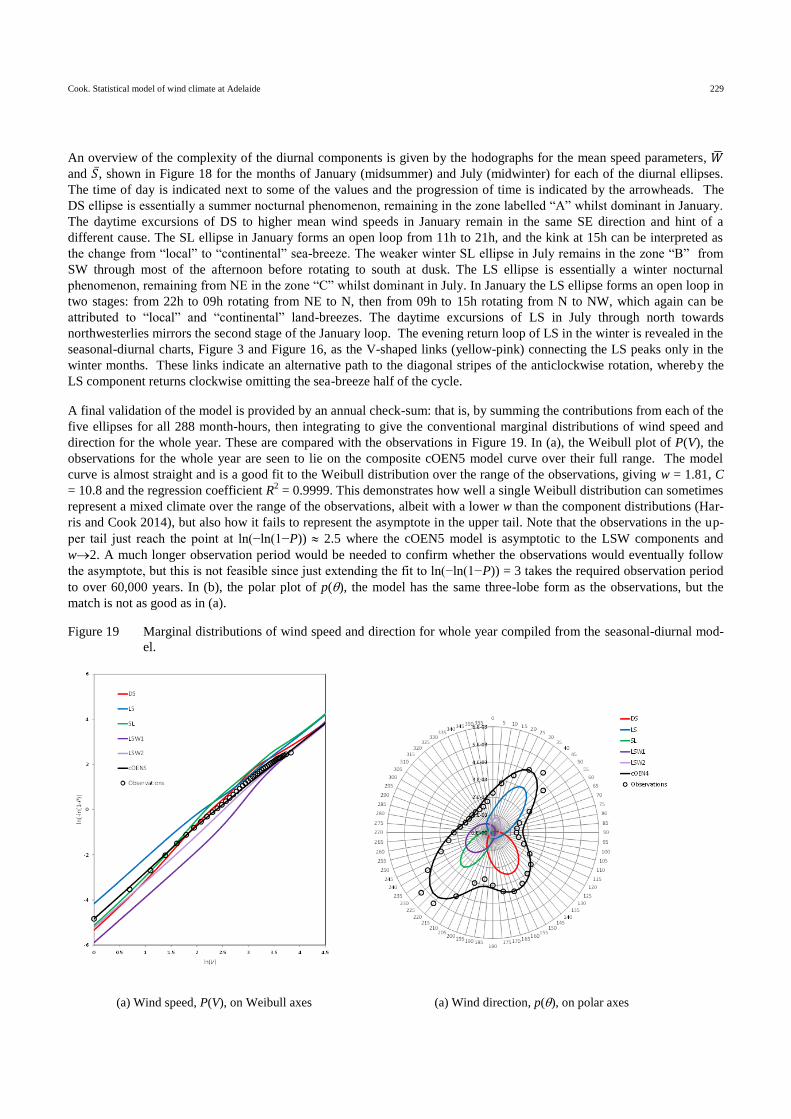
A final validation of the model is provided by an annual check-sum: that is, by summing the contributions from each of the

five ellipses for all 288 month-hours, then integrating to give the conventional marginal distributions of wind speed and

direction for the whole year. These are compared with the observations in Figure 19. In (a), the Weibull plot of P(V), the

observations for the whole year are seen to lie on the composite cOEN5 model curve over their full range. The model

curve is almost straight and is a good fit to the Weibull distribution over the range of the observations, giving w = 1.81, C

= 10.8 and the regression coefficient R2 = 0.9999. This demonstrates how well a single Weibull distribution can sometimes

represent a mixed climate over the range of the observations, albeit with a lower w than the component distributions (Har-

ris and Cook 2014), but also how it fails to represent the asymptote in the upper tail. Note that the observations in the up-

per tail just reach the point at ln(−ln(1−P)) 2.5 where the cOEN5 model is asymptotic to the LSW components and

w2. A much longer observation period would be needed to confirm whether the observations would eventually follow

the asymptote, but this is not feasible since just extending the fit to ln(−ln(1−P)) = 3 takes the required observation period

to over 60,000 years. In (b), the polar plot of p(), the model has the same three-lobe form as the observations, but the

match is not as good as in (a).

Figure 19 Marginal distributions of wind speed and direction for whole year compiled from the seasonal-diurnal mod-

el.

(a) Wind speed, P(V), on Weibull axes (a) Wind direction, p(), on polar axes


The LSW1 and LSW2 ellipses merge to produce a common asymptote and the diurnal downslope ellipse, DS, also merges

into the asymptote further up the tail. This upper tail asymptote is very well represented by a Weibull distribution (Eqn. 1)

with w = 1.94 and C = 12.1 kn, comparing well with the expectation of w = 2 from the theory underpinning the OEN mod-

el (Harris and Cook 2014). This behaviour is crucial in the design of structures to resist extreme winds and its compliance

with the expected asymptotic behaviour means that the OEN model is compatible with the current extreme-value and

peak-over-threshold methods on which current wind engineering design practice is based.

Being a phenomenological black-box model, the smoothed OEN model is a simplification of reality which meets the prin-

cipal aim of prediction and simulation of the Adelaide wind climate sufficiently well for engineering design. It is likely

that there is still more useful information lurking in the data that might be extracted to further the second aim of elucidat-

ing the meteorological mechanisms. For example, the minor peak marked “A” in Figure 7(c) for July appears to indicate a

non-diurnal NE drift which is present from May through to August. This suggests that the persistence of the LS ellipse

through winter afternoons discussed earlier might be due to a synoptic-scale mechanism that adds to the nocturnal land-

breeze to form the LS ellipse. The same argument applies to the persistence of the DS ellipse through summer afternoons

and the corresponding low-frequency strong SE excursions, especially as the DS component merges with the LSW com-

ponents in the upper tail of Figure 19(a).

Clearly this black-box model could be further improved, or “whitened”, by the addition of more independent knowledge

about the Adelaide climate, but the gleaning of further insights is left to the reader.

Conclusions

The seasonal-diurnal variation in wind speed and direction at Adelaide, SA, has been represented by the disjoint

sum of k 5 bivariate normal distributions, where each k represents one of five physical wind mechanisms indi-

cated by the observations “speaking for themselves”.

The OEN methodology, which uses parameter optimisation, is able to deduce the k distributions from the ob-

served distribution of the wind vector in the zonal-meridional plane, p(W,S), even when the component distribu-

tions overlap.

Bootstrapping simulated trials of the observations shows the OEN methodology to be robust when the relative

frequency of a component f > 0.1.

Optimising all parameters together results in a model where the k distributions are an arbitrary linear combination

of the wind climate mechanisms. Elucidating the physical climate mechanisms requires one bivariate normal dis-

tribution to be assigned to each climate component and the parameters to be conditionally optimised, iteratively.

Bootstrapping demonstrates that the conditionally optimised distributions are not arbitrary combinations.

The five climate components found at Adelaide correspond to the three seasonal-diurnal components: downslope

winds from the Adelaide Hills, sea-to-land breezes and land-to-sea breezes; and to two seasonal, non-diurnal

components corresponding to winter- and summer-dominating large-scale weather systems. There may be other

components that have not been found or have been subsumed into the five components, e.g. a winter daytime NE

drift.

The parameters defining the five bivariate normal distributions are adequately represented by just the mean, an-

nual, semi-annual, diurnal and semi-diurnal harmonics.

The joint statistics of wind speed and direction at Adelaide have been quantified by a single statistical model con-

sistent with the observed meteorological processes.

The OEN model is easily implemented in statistical simulations using standard “bootstrapping” methods, in

which case the simulated observations are uncorrelated and in arbitrary order.

This is a step towards the ultimate aim of time-series simulations. Next steps are the derivation of additional

models for the serial correlation between adjacent hours and of the switching between the climate mechanisms.

This is the subject of future work.

Acknowledgments

This paper was prepared and the underlying study was conducted as personal, self-funded research by the sole author.

The author thanks Mr R I Harris for his principal role in the development of the OEN model and the many helpful conver-

sations on its application to mixed wind climates. The author also thanks the two referees of the original draft for their


comments on the intricacies of the Adelaide climate and their helpful suggestions for re-structuring the paper for a meteor-

ological audience.

References

Brittain, O. W. 1966. A method for forecasting the sea breeze at Manby. Meteorological Office Forecasting Techniques,

Memorandum 12, 6–16.

Brooks, C. E. P., Durst, C. S. and Carruthers, N. 1946. Upper winds over the World, Part I, The frequency distribution of

winds at a point in the free air. Q. J. Roy. Meteor. Soc., 72, 55–73

Clarke, R.H. 1955. Some observations and comments on the sea breeze. Aust. Met. Mag., 11, 47–68

Cook, N.J. 2004. Confidence limits for extreme wind speeds in mixed climates. J. Wind Engng. Indust. Aerodyn., 92, 41–

51

Cook, N. J. 2012. The atmospheric tide and the sea-land breeze cycle in Jersey. Weather, 67, 184–187

Cook, N. J. 2014a. Review of errors in archived wind data. Weather, 69, 3, 72-81. doi: 10.1002/wea.2148.

Cook, N. J. 2014b. Detecting artefacts in analyses of extreme wind speeds. Wind and Structures, 19, 271–294. doi:

10.12989/was.2014.19.3.271.

Cook, N. J. 2015. Visualising seasonal-diurnal trends in wind observations, Weather, 70, 111–115. doi:10.1002/wea.2357.

Crutcher, H. L. 1957. On the standard vector-deviation wind rose. J. Meteorol., 14, 28–33

Crutcher, H.L. and Baer, L. 1962. Computations from elliptical wind statistics, J. Appl. Meteorol., 1, 522–530

Crutcher, H. L. and Joiner, R.L. 1977a. Separation of mixed data sets into homogeneous sets, NOAA Technical Report

EDS 19, Dept. of Commerce, Washington DC, 167 pp.

Crutcher, H.L. and Joiner, R.L. 1977b. Another look at the upper winds of the tropics, J. Appl. Meteorol., 16, 426–476

Dai, A. and Deser, C. 1999. Diurnal and semidiurnal variations in global surface wind and divergence fields. J. Geophys.

Res., 104, 109–131.

Dexter, R. V. 1958. The sea-breeze hodograph at Halifax, Bull. Amer. Meteorol. Soc., 39, 241–247.

Efron, B. and Tibshirani, R. J. 1993. An introduction to the bootstrap, New York, Chapman and Hall, 436 pp, ISBN 978-

0-412-04231-7

Ferriere, P. J. 1994. Weather Hazards at Adelaide Airport. Met. Note 204. Australian Bureau of Meteorology, 35 pp.

Grace, W. and Holton, I. 1990. Hydraulic jump signatures associated with Adelaide downslope winds. Aust. Met. Ocean-

ogr. J., 38, 43−52.

Haurwitz, B. 1947. Comments on the sea-breeze circulation, J. Meteorol., 4, 164−165.

Harris, R. I. 2014. A simulation method for the macro-meteorological wind speed and the implications for extreme value

analysis, J. Wind Engng. Indust. Aerodyn, 125, 146−155.

Harris, R. I. and Cook, N. J. 2014. The parent wind speed distribution: Why Weibull?, J. Wind Engng. Indust. Aerodyn,

131, 72−87.

Jakob, D. 2010. Challenges in developing a high-quality surface wind-speed data-set for Australia. Aust. Met. Oceanogr.

J., 60, 227−236.

Kusada, M. and Alpert, P. 1983. Anti-clockwise rotation of the wind hodograph. Part I: Theoretical study, J. Atmos. Sci.,

40, 487−499.

Lanczos, C. 1956. Applied analysis. Prentice Hall, Englewood Cliffs, New Jersey.

Moisseeva, N. and Steyn, D. G. 2014. Dynamical analysis of sea-breeze hodograph rotation in Sardinia. Atmos. Chem.

Phys., 14, 13471−13481.

Naess, A. and Clausen, P. H. 2001. Combination of the peaks-over-threshold and bootstrapping methods for extreme value

prediction. Struct. Saf., 23, 315−330.

Peel, M. C., Finlayson, B. L. and McMahon, T.A. 2007. Updated world map of the Köppen-Geiger climate classification.

Hydrol. Earth Syst. Sci., 11, 1633–1644.

Physick, W.L. and Byron-Scott, R. A. D. 1977. Observations of the sea breeze in the vicinity of a gulf. Weather, 32,

373−381.

Sha, W., Grace, W. and Physick, W. 1996. A numerical experiment on the Adelaide gully wind of South Australia. Aust.

Met. Mag.,45, 19−40.

Simpson, J. E. 1996. Diurnal changes in sea-breeze direction. J. Appl. Meteorol, 35, 1166−1169.

Staley, D. O. 1957. The low-level sea breeze of northwest Washington. J. Meteorol., 14, 458−470.

Staley, D. O. 1989. The surface sea breeze: Applicability of Haurwitz-type theory. J. Appl. Meteorol., 28, 137–145.


Steyn, D. G. and Kallos, G. 1992. A study of hodograph rotation in the sea breezes of Attica, Greece. Bound.-Lay. Mete-

orol., 58, 215−228.

Tepper, G. and Watson, A. 1990. The wintertime nocturnal northeasterly wind of Adelaide, South Australia: an example of

topographic blocking in a stably stratified air mass, Aust. Met. Mag., 38, 281−291.

Torrielli, A., Repetto, M. P. and Solari, G. 2013. Extreme wind speeds from long-term synthetic records, J. Wind Engng.

Indust. Aerodyn., 115, 22−38.

Torrielli, A., Repetto, M. P. and Solari, G. 2014. A refined analysis and simulation of the macro-meteorological wind

components, J. Wind Engng. Indust. Aerodyn., 132, 54−65.

A statistical model of the seasonal-diurnal wind climate ... · A statistical model of the...

Documents

Transcript of A statistical model of the seasonal-diurnal wind climate ... · A statistical model of the...