A statistical model for 1-hour- to 24-hour-ahead ... · concerned with the prediction of hourly...

A statistical model for 1-hour- to 24-hour-aheadprediction of hourly ozone concentrations atground level in Singapore

X. Liu1, Y. Hwang2, K. Yeo2, J. Hosking2, A. Barut2,J. Singh1 & Y. Amemiya2

1IBM Research Collaboratory Singapore, Singapore2IBM Thomas J. Watson Research Center, USA

Abstract

A spatio-temporal statistical model is proposed for 1- to 24-hour-ahead predictionof hourly ozone concentrations. This is a joint work with the NationalEnvironmental Agency Singapore, and is Singapore’s first predictive model forozone concentrations. Unlike many existing models which focus on either dailymaximum or 8h average daylight ozone concentrations, the present work isconcerned with the prediction of hourly ozone concentrations which are usuallyassociated with higher variability. A recently proposed framework for spatio-temporal prediction is used to model ozone concentration data. The macro-scale spatio-temporal variation of ozone concentrations is modeled by a linearfunction of five carefully constructed predictors, while the micro-scale variation iscaptured by a mean-zero spatio-temporally correlated random process. We showthat this model also provides useful insights about the effects of some complexenvironmental processes on ozone concentration; this is indeed an attractivefeature for any data-driven air quality model.Keywords: ozone, spatio-temporal statistics, random process.

1 Introduction

Ground-level ozone is one of the major air pollutants regulated by the U.S.Clean Air Act [1] as well as the air quality guidelines of the World HealthOrganization [2]. Although the upper-atmosphere ozone layer shields us from

Air Pollution XXII 389

www.witpress.com, ISSN 1743-3541 (on-line) WIT Transactions on Ecology and The Environment, Vol 183, © 2014 WIT Press

doi:10.2495/AIR140321

the harmful ultraviolet rays, ground-level ozone is usually harmful. When ozoneis inhaled, it irritates the respiratory system, inflames and damages the liningof the lungs, increase the susceptibility to respiratory infections, etc. When the8-hour concentration exceeds 240µg/m3, both healthy adults and asthmaticsexperience significant reductions in lung function [2, 3]. The Air Quality Index(AQI) is considered good or moderate when the 8-hour mean ozone concentrationis not higher than 0.08 parts per million, which is approximately 169µg/m3. TheSingapore National Environmental Agency (NEA) adopts the WHO guidelines andset the target for 8-hour mean ozone concentration to 100µg/m3.

Ozone is formed in the atmosphere by photochemical reactions in the presenceof sunlight and precursor pollutants, such as the oxides of nitrogen (NOx) andvolatile organic compounds (VOCs). It is destroyed by reactions with NO and isdeposited to the ground. Several studies have shown that ozone concentration iscorrelated with various toxic photochemical oxidants arising from similar sources,including the peroxyacyl nitrates, nitric acid and hydrogen peroxide [4].

As a joint work between IBM Research and Singapore NEA, we propose inthis paper a novel statistical model to predict the hourly average ground-levelozone concentrations 1 to 24 hours in advance. This is Singapore’s first predictivemodel for ozone concentrations. Although various methods have been proposedto model ozone concentrations (see [5] for a comprehensive survey), most of theexisting methods focus on either the daily maximum or daylight 8-hour averageozone concentration [6–8]. In this research, we focus on the prediction of hourlyozone concentrations, which is more challenging as ozone concentrations at hourlylevel are usually associated with higher uncertainty. Furthermore, the study areaconsidered in this work, i.e., Singapore, is much smaller than that of many existingstudies and is characterized by a dense built-up urban area. Hence, being able tomodel the local spatio-temporal variability of ozone concentrations becomes morecritical.

For the past decades, spatio-temporal statistics have been widely employed inmodeling air quality data [8–10]. In these studies, pollutants concentrations aremodeled by some random field. Assumptions such as stationary covariance andisotropy (i.e., covariance function only depends on distance) are often empiricallymade so as to keep the model mathematically tractable. These assumptions mightbe appropriate when data are aggregated over a relatively large area or long timeperiod. For hourly-level data, however, assumptions like stationary covarianceand isotropy rarely hold due to the high variability associated with hourly ozoneconcentrations and meteorological conditions. In fact, such commonly madeassumptions may not even be validated using statistical approaches unless dataarise from a large number of air quality monitoring stations [11]. To relax suchlimitations, this study employs a spatio-temporal prediction framework recentlydeveloped by researchers from IBM Watson Research Center [12]. Our studyshows that this framework can effectively model ozone concentration and wellbalances the complexity and the practicality of a spatio-temporal predictionapproach. In Section 2, we describe the study area and the data used to constructthe model. Section 3 provides the modeling details. Results of model testing are

390 Air Pollution XXII


103.6°E 103.7°E 103.8°E 103.9°E 104°E 104.1°E

1.1°N

1.2°N

1.3°N

1.4°N

1.5°N

air quality stationsmeteorological stations

Figure 1: Locations of air quality and meteorological stations in Singapore.

summarized in Section 4. It is also noted that, the model constructed can beinterpreted in terms of the basic physics and chemistry of ozone; this is indeedan attractive feature for a data-driven air quality model, and discussions can befound in Section 4.

2 Study area and data

2.1 Study area

As a tropical island country located 137km north of the equator, Singapore has atotal land area of 716.1km2 and a population close to 5.4 million. The populationdensity is 7, 669/km2 and ranked the 3rd highest in the world [13]. The motorvehicle population has also reached 974,170 by the end of 2013 [14], and theannual mean temperature typically ranges from 24◦C to 32◦C, creating the idealconditions for ozone to be generated.

2.2 Data

Hourly-level ozone concentrations (µg/m3) measured at seven air qualitymonitoring stations are available for our study. In this paper, we focus on the data



hour of day

conc

entra

tion,

(µ g

/m3 )

0 6 12 18

0

10

20

30

40

50

60

70 Stn−1Stn−2Stn−3Stn−4Stn−5Stn−6Stn−7

Figure 2: Diurnal variation of ozone concentrations.

collected from 8am 01/06/2013 to 7am 30/08/2013 (Singapore local UTC+08:00time zone). Locations of stations are shown in Figure 1. Approximately 5.5% ofthe ozone measurements are missing and the occasions of no measured data aredue to system under maintenance. Figure 2 displays the mean ozone concentrationat a given hour of a day and for all seven stations. The diurnal ozone concentrationis mainly due to the fact ozone can only be generated under sunlight. The spatialvariation, on the other hand, is much more dynamic since it depends on factorssuch as traffic, wind direction and speed, land use, hour of a day and so on.

Temperature, wind speed and wind direction are also available at meteorologicalstations. Locations of these stations are shown in Figure 1. Note that, air qualitystations and meteorological stations do not share same locations, and therefore,spatial interpolation of meteorological conditions is needed. This is appropriatewhen the density of meteorological stations is high, just as in our case.

Land use information is also used in our modeling, but we leave the detaileddescription and processing of these datasets in Section 3.2.

3 The model

3.1 The general framework

Let ozt(s) be the ozone concentration at location s and time t, where the spatiallocation s is defined as a vector of its coordinates under SVY21 coordinated



cadastre system. Because the distribution of ozone concentration is right-skewed,we model the square root transformation of ozt(s) as follows:

Yt(s) =√

ozt(s) = gt(s) + Zt(s) (1)

where s ∈ {s1, s2, . . . , sn} and t = 1, . . . ,m. In equation (1), gt(s) is adeterministic function which captures the macro-scale spatio-temporal trend ofozone concentration, and Zt(s) is a mean-zero spatio-temporal correlated randomprocess which captures the micro-scale spatio-temporal variation. Details of themodeling of gt(s) and Zt(s) are provided in sections 3.2 and 3.3, respectively,

3.2 The deterministic spatio-temporal trend

The macro-scale spatio-temporal trend of ozone concentration are influenced byfactors such as land use, temperature, wind, etc. Being able to build the rightmodel for gt(s) largely determines whether the spatio-temporal variation of theozone concentrations can be accurately predicted. In fact, sophisticated treatmentof the random component Zt(s) might not yield a substantial payoff for predictionaccuracy [12].

We model gt(s) as a linear function of five predictors as follows:

gt(s) = x(land)t (s)β(land) + x(upwind)

t (s)β(upwind)

+ x(temp)t (s)β(temp) + x(ws)

t (s)β(ws) + x(hour)t (s)β(hour)(2)

The first predictor x(land)t (s) is constructed from the land use of Singapore.Different types of land use to a large extent determine the macro-scale spatialtrend of ozone emissions [15]. In the raw dataset of land use, Singapore isdivided into 110830 spatial polygons with 32 categories of land use. To modelthe spatial and temporal patterns of ozone in downtown and suburb, industrialand residential, urban and nature reserve areas, as well as the local reduction ofozone concentrations due to traffic-induced NO-scavenging, we re-group the 32categories into five main land use types, including residential, road, nature reserve,commercial and industrial.

For any location s and land use type i (i = 1, 2, . . . , 5), we define the landuse index l(i)(s) as the total spatial area of land use of type i within 5km radiusof location s. As an illustration, Figure 3a and 3b respectively show the land useindex for industrial areas (i.e., l(5)) and residential areas (i.e., l(1)) for Singapore.Here, each pixel has an area of 0.7km2.

Our exploratory analysis also suggests that different types of land use havedifferent effects on ozone concentrations at different hours of a day. Hence, letτ(t) be a function that returns the hour of a calendar time t (τ(t) ∈ (1, 2, . . . , 24)),we construct the predictor x(land)

t (s) based on the land use index as follows:

x(land)t (s) ={

x(landi)t (s)

}5

i=1(3)



0

5

10

15

20

25

30

35

40

(a)

0

10

20

30

40

(b)

0

500

1000

1500

2000

2500

3000

(c)

0

500

1000

1500

2000

(d)

Figure 3: (a) Land use index for industrial areas (km2); (b) Land use index forresidential areas (km2); (c) Upwind land use index for industrial areas (km2);(d) Upwind land use index for residential areas (km2). For (c) and (d), the windspeed equals 8.4km/hour and the wind direction equals 227o.

Our exploratory analysis also suggests that different types of land use havedifferent effects on ozone concentrations at different hours of a day. Hence, letτ(t) be a function that returns the hour of a calendar time t (τ(t) ∈ (1, 2, . . . , 24)),we construct the predictor x(land)t (s) based on the land use index as follows:

x(land)t (s) ={

x(landi)t (s)

}5

i=1(3)

and the jth (j = 1, 2, . . . , 24) component of x(landi)t (s) is given by

x(landi)t,j (s) =

{l(i)(s), j = τ(t)

0, otherwise(4)

The second predictor x(upwind)t (s) accounts for the emissions transported

downwind. We adopt and extend the idea in [11] and define the upwind land useindex x(upwind)(s). Let wt be the island-wide mean wind vector for Singapore at

Figure 3: (a) Land use index for industrial areas (km2); (b) Land use index forresidential areas (km2); (c) Upwind land use index for industrial areas(km2); (d) Upwind land use index for residential areas (km2). For (c)and (d), the wind speed equals 8.4km/hour and the wind directionequals 227o.

and the jth (j = 1, 2, . . . , 24) component of x(landi)t (s) is given by

x(landi)t,j (s) =

{l(i)(s), j = τ(t)

0, otherwise(4)

The second predictor x(upwind)t (s) accounts for the emissions transported

downwind. We adopt and extend the idea in [11] and define the upwind land useindex x(upwind)(s). Let wt be the island-wide mean wind vector for Singapore attime t, and let vt denote the wind speed. Then, for any location s0 and land usetype i (i = 1, 2, . . . , 5), the upwind land use index l̃(i)(s) is defined as the totalarea of land use of type i within an upwind cone S defined by

S =

{s : |s− s0| 6 vtρ,

|(s− s0)wt|vt

> |s− s0| cos(α/2),−(s− s0)wt

vt< 0

}

For any particular location s0, S is an upwind cone with radius proportional towind speed. The arc of the cone is determined by α and is to capture the variation



of wind directions. Unlike the static land use index, the upwind land use indexis dynamic as wind changes its speed and direction. As an illustration, the leftand right panels of Figure 3c and Figure 3d respectively show the upwind landuse index for industrial areas (i.e., l̃(5)) and for residential areas (i.e., l̃(1)) forSingapore, given that the wind speed equals 8.4km/hour and the wind directionequals 227o.

The upwind land use index also has different effects on ozone concentrations atdifferent hours of a day. Similarly, we construct the predictor x(upwind)

t (s) basedon the upwind land use index as follows:

x(upwind)t (s) =

{x(upwindi)t (s)

}5

i=1(5)

and the jth (j = 1, 2, . . . , 24) component of x(upwindi)t (s) is given by

x(upwindi)t,j (s) =

{l̃(i)(s), j = τ(t)

0, otherwise(6)

The third predictor x(temp)t is obtained from the temperature at time t and

location s. Since ozone is only generated during daylight, temperature at nightdoes not significantly affect ozone concentrations. Hence, we construct x(temp)

t (s)as follows:

x(temp)t (s) =

{Tt(s), if τ(t) ∈ (8, 9, . . . , 19)

0 if τ(t) ∈ (1, . . . , 7) ∪ (20, . . . , 24)(7)

where Tt(s) is the temperature at time t and location s.The fourth predictor x(ws)

t is constructed from the island-wide mean wind speedvt at time t. It is mainly used to capture the dilution of ozone concentrations atnight due to wind. Hence, we construct x(ws)

t (s) as follows:

x(ws)t (s) =

{vt, if τ(t) ∈ (1, 2, . . . , 7) ∪ (20, . . . , 24)

0 if τ(t) ∈ (8, . . . , 19)(8)

The last predictor x(hour)t (s), which is given by equation (9), accounts for thehourly effect of ozone concentration of a day.

x(hour)t,j (s) =

{1, j = τ(t)

0, otherwise(9)

where x(hour)t,j (s) is the jth component of x(hour)t (s), and j = 1, 2, . . . , 24.



3.3 The spatio-temporal random process

Following the idea of [12], the spatio-temporal process in equation (1), Zt(s), ismodeled as an autoregressive (AR) model of order L

Zt(s) =L∑

l=1

γlZt−l(s) + ε(s) (10)

with the AR residuals, ε = (ε(s1), ε(s2), . . . , ε(sn)), being a mean-zero, second-order stationary and isotropic stochastic random field, i.e.,E(ε) = 0 and V ar(ε) =Σ = (Σ)i,j=1,2,...,n. Here, an Exponential spatial covariance function is adopted

Σi,j = Cov(ε(si), ε(sj)) =

{σ2 exp(−θhi,j), hi,j > 0

σ2 + κ2, hi,j = 0(11)

where hi,j = ‖si − sj‖ is the distance between site si and sj for i, j = 1, 2, . . . , n,κ is known as the nugget effect in spatial statistics, and θ is an unknown parameter.

Hence, the spatio-temporal process Z = (Zt−L+1(s), . . . , Zt(s)) has aseparable space-time covariance function such that

V ar(Z) = Γ⊗

Σ (12)

where Γ is the AR(L) covariance matrix.

4 Model evaluation and discussions

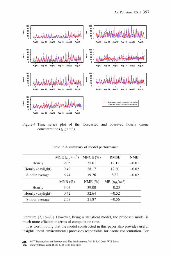
The model is evaluated using the data collected from 8am 01-June-2013 to 7am 30-Aug-2013, including the observed hourly ozone concentrations, observed hourlyweather data, Numerical Weather Prediction (NWP) data and land use data.Starting from 7am 01-July-2013, predictions of hourly ozone concentrations forthe next 24 hours (i.e., from 8am to 7am next day) are generated and compared tothe observed ozone concentrations. The model is run on daily basis till 7am 29-Aug-2013, and model parameters are dynamically re-estimated using the data inthe most recent 168 hours.

With reference to the performance metrics recommended by USEPA [5,16] andUK DEFRA [17] for evaluation of air quality models, the following metrics areused: Mean Normalized Gross Error (MNGE), Mean Gross Error (MGE), Root-Mean-Square Error (RMSE), Normalized Mean Bias (NMB), Mean NormalizedBias (MNB), Normalized Mean Error (NME) and Mean Bias (MB). Table 1shows the values for above performance metrics for our model. As an illustration,Figure 4 shows both the predicted and observed hourly pollutant concentrations inAugust.

Results presented in Table 1 show that the accuracy of the proposed modelis comparable to that of many existing models, such as CMAQ, reported in the



Aug 03 Aug 08 Aug 13 Aug 18 Aug 23 Aug 28

020406080

100

Stn

−1


020406080

100

Stn

−1


020406080

100

Stn

−2


020406080

100

Stn

−2


020406080

100

Stn

−3


020406080

100

Stn

−3


020406080

100

Stn

−4


020406080

100

Stn

−4


020406080

100

Stn

−5


020406080

100

Stn

−5


020406080

100

Stn

−6


020406080

100

Stn

−6


020406080

100

Stn

−7


020406080

100

Stn

−7 forecasted hourly ozone concentrationobserved hourly ozone concentration

Figure 4: Time series plot of the forecasted and observed hourly ozoneconcentrations (µg/m3).

Table 1: A summary of model performance.

MGE (µg/m3) MNGE (%) RMSE NMBHourly 9.05 35.61 12.12 −0.01

Hourly (daylight) 9.49 28.17 12.80 −0.02

8-hour average 6.74 19.76 8.82 −0.02

MNB (%) NME (%) MB (µg/m3)Hourly 3.03 39.00 −0.23

Hourly (daylight) 0.42 32.64 −0.52

8-hour average 2.57 21.87 −0.56

literature [7, 18–20]. However, being a statistical model, the proposed model ismuch more efficient in terms of computation time.

It is worth noting that the model constructed in this paper also provides usefulinsights about environmental processes responsible for ozone concentration. For



hour of day

0 6 12 18

−0.30

0.09residential

hour of day

0 6 12 18

−1.5

−0.7roads

hour of day

0 6 12 18

−0.05

0.05nature reserve

hour of day

0 6 12 18

0.6

1.8

commercial

hour of day

0 6 12 18

−0.10

0.08industrial

Figure 5: Effects of different land use on ozone concentrations.

illustration purposes, Figure 5 shows the estimated effects of different land use onozone concentrations based on the data from Aug 8 to Aug 15. We see that:• Higher residential land use and road density generally result in lower ozone

concentrations. As the exhaust fumes of vehicles are the main anthropogenicsource of oxides of nitrogen (NO), an increase in NO concentrations causea decrease in ozone concentrations (i.e., NO-scavenging [11]). In fact, itis possible to see that the negative effect of residential area on ozoneconcentrations becomes stronger at 7am and 8am during the morning rushhour. In addition, because ozone cannot be formed without solar radiation,the negative effect of road density on ozone concentrations also becomesstronger at night.• The effects of nature reserve land use type and industrial land use type have

similar effects on ozone concentration over a day. Both land use types havenegative effects on ozone concentrations during night, but positive effect onozone concentrations during daylight. This is primarily because ozone isdestroyed at night by NO at night, especially in industrial areas.• The commercial land use type have positive effects on ozone concentrations.

This implies that the ozone concentration is higher in downtown Singaporewhere most of the land is for commercial use. Because of the high NOconcentration during daylight, the effect of commercial land use on ozoneconcentrations becomes weaker during daylight.

5 Conclusions

A statistical model has been proposed for predicting hourly ozone concentrations,and this is the first predictive model for ozone concentrations for Singapore. Boththe mathematical formulation and testing results were presented in this paper. It



has been shown that the accuracy of the proposed model is comparable to that ofmany existing models. Our next step is to test the proposed model on a continualdaily basis and explore the modeling of other pollutants under a similar framework.

References

[1] US Environmental Protection Agency, Clean air act – air pollutionprevention and control, 2012.

[2] World Health Organization, WHO air quality guidelines for particulatematter, ozone, nitrogen dioxide and sulfur dioxide – global update,WHO/SDE/PHE/OEH/06.02, 2005.

[3] US Environmental Protection Agency, Air quality index - a guide to airquality and your health, EPA-454/K-03-002, 2003.

[4] Han, S., Bian, H., Feng, Y., Liu, A., Li, X., Zeng, F. & Zhang, X., Analysisof the relationship betweenO3,NO andNO2 in Tianjin, China. Aerosol andAir Quality Research, 11, pp. 128–139, 2011.

[5] US Environmental Protection Agency, Guidelines for developing an airquality (ozone and PM2.5) forecasting program, EPA-456/R-03-002, 2003.

[6] Davis, J.M. & Speckman, P., A model for predicting maximum and 8haverage ozone in Houston. Atmospheric Environment, 33, pp. 2487–2500,1999.

[7] Wang, W., Lu, W., Wang, X. & Leung, A., Prediction of maximum dailyozone level using combined neural network and statistical characteristics.Environment International, 29, pp. 555–562, 2003.

[8] Bogaert, P., Chistakos, G., Jerrett, M. & Yu, H.L., Spatiotemporal modellingof ozone distribution in the state of California. Atmospheric Environment, 43,pp. 2471–2480, 2009.

[9] Carroll, R.J., Chen, R., George, E.I., Li, T.H., Newton, H.J., Schmiediche, H.& Wang, N., Ozone exposure and population density in Harris county, Texas.Journal of the American Statistical Association, 92, pp. 392–404, 1997.

[10] Chistakos, G. & Vyas, V.M., A composite space/time approach to studyingozone distribution over eastern United States. Atmospheric Environment, 16,pp. 2845–2857, 1998.

[11] Abraham, J.S. & Comrie, A.C., Real-time ozone mapping using a regression-interpolation hybrid approach applied to Tucson Arizona. Journal of the Airand Waste Management Association, 45, pp. 914–925, 2004.

[12] Jiang, H.J., Schorgendorfer, A., Hwang, Y. & Amemiya, Y., A practicalapproach to spatio-temporal analysis. Statistica Sinica, submitted, 2014.

[13] Singapore Department of Statistics, Population in brief, 2013.[14] Singapore Department of Statistics, Monthly digest of statistics Singapore,

2014.[15] Xu, Y., Vizuete, W. & Serre, M., Characterization of air quality ozone model

performance using land use regression model: An application in exposureassessment for epidemiology studies. the 11th Annual CMAS Conference,Chapel Hill, North Carolina, 2012.



[16] Air quality modeling technical support document. US EnvironmentalProtection Agency, EPA-454/R-11-009, 2011.

[17] UK Department for Environment Food and Rural Affairs, Evaluating theperformance of air quality models, 2010.

[18] Arasa, R., Soler, M.R., Olid, M. & Merino, M., A performance evaluationof MM5/MNEQA/CMAQ air quality modelling system to forecast ozoneconcentrations in Catalonia. Journal of Mediterranean Meteorology andClimatology, 7, pp. 11–23, 2010.

[19] Eder, B., Kang, D., Mathur, R., Yu, S. & Schere, K., An operationalevaluation of the ETA-CMAQ air quality forecast model. AtmosphericEnvironment, 40, pp. 4894–4905, 2006.

[20] Pires, J.C.M., Alvim-Ferraz, M.C.M., Pereira, M.C. & Martins, F.G.,Comparison of several linear statistical models to predict tropospheric ozoneconcentrations. Journal of Statistical Computation and Simulation, 82, pp.183–192, 2012.



A statistical model for 1-hour- to 24-hour-ahead ... · concerned with the prediction of hourly...

Documents

Transcript of A statistical model for 1-hour- to 24-hour-ahead ... · concerned with the prediction of hourly...