A statistical approach to optimal target detection and

localization in the presence of noise

Habib Ammari∗ Josselin Garnier† Knut Sølna‡

May 30, 2010

Abstract

The problem addressed in this paper is the combined detection and localiza-tion of a point reflector embedded in a medium by sensor array imaging whenthe array response matrix is measured in a noisy environment. We constructa detection test based on reverse-time migration of the array response matrixthat is the most powerful for a given false alarm rate and prove that it is moreefficient than the one introduced in [3], which is based on the singular valuedecomposition of the response matrix. Moreover, we show that reflector local-ization should be performed with reverse-time migration rather than any otherform of weighted-subspace migration and we give the standard deviation of thelocalization error.

1 Introduction

The problem addressed in this paper is to detect and localize a point reflector embed-ded in a medium by probing the medium with time-harmonic scalar waves emittedfrom and recorded on a sensor array. We use stochastic and statistical tools to studythis problem when the array response matrix is acquired in a noisy environment.We consider a clutter noise (small random fluctuations in the background medium)in the multiple scattering regime and an additive measurement noise. In both situ-ations, up to a symmetrization of the response matrix, the noise can be modeled bya symmetric Gaussian matrix with zero mean.

Our first goal is to design an optimal detection procedure. Using the Neyman-Pearson Lemma [13], we construct a detection test based on reverse-time migrationof the array response matrix that is the most powerful for a given false alarm rate.

∗Department of Mathematics and Applications, Ecole Normale Superieure, 45 Rue d’Ulm, 75005Paris, France (habib.ammari@ens.fr).

†Laboratoire de Probabilites et Modeles Aleatoires & Laboratoire Jacques-Louis Lions, Univer-site Paris VII, 2 Place Jussieu, 75251 Paris Cedex 5, France (garnier@math.jussieu.fr).

‡Department of Mathematics, University of California, Irvine, CA 92697 (ksolna@math.uci.edu).

1

We compare this test with the one introduced in [3], which is based on the singularvalue decomposition (SVD) of the noisy response matrix. We show that it is moreefficient than the SVD-based test because it uses the known structure of the singularvector associated to the point reflector while the SVD-based test does not exploitthis structure.

The second aim of this paper is to provide weighted subspace migration func-tionals for localizing the point reflector and compare their performance. We showthen the optimality of the reverse-time migration imaging functional in the presenceof noise.

It is expected that by combining the asymptotic formalism provided in [2, 4,5] together with the recent results on low-rank perturbations of random Gaussianmatrices [11, 12, 15], we can extend the results of this paper to the detection andlocalization of small inclusions. Response matrices obtained in the presence of smallinclusions and cracks have, in general, more than one significant singular value.

The paper is organized as follows. In Sections 3-4 we propose two detectiontests, one based NB on the SVD of the array response matrix and anotherbased on the reverse-time migration functional of the response matrix.We study general versions of these tests using random matrix theory, in particularrecent results on low-rank perturbations of random Gaussian matrices, and extremevalue theory for Gaussian fields. We identify the most powerful tests using Neyman-Pearson Lemma and we show that the levels of the tests are prescribed in termsof a Tracy-Widom distribution or a Gumbel distribution. Quantitative calculationsallow us to describe the regimes in which the migration-based test is more powerfulthan the SVD-based test. In Section 5 we identify the optimal migration techniquefor estimating the location of the reflector in the presence of additive noise by usinga Bayesian approach. We find that reverse-time migration is slightly more robustthan Kirchhoff migration [7], and that both are much more robust than algorithmsof MUSIC-type (which stands for MUltiple SIgnal Classification; see [8, 14, 17, 22]).We compute the standard deviation of the error in the localization for the optimalreverse-time migration technique.

2 Problem formulation

Let us assume that the background medium is homogeneous with speed of propaga-tion c0. For a given frequency ω, let G0(ω,x,y) be the outgoing Green function for∆x +ω2/c2

0 in Rd corresponding to a Dirac mass at y. That is, G0 is the solution to

∆xG0 +ω2

c20

G0 = −δy(x) in Rd, d = 2 or 3,

2

subject to the outgoing radiation condition. In three dimensions, the Green functionis given by

G0(ω,x,y) =ei ω

c0|x−y|

4π|x − y| ,

while in two dimensions,

G0(ω,x,y) =i

4H

(1)0

( ω

c0|x|

)

,

where H(1)0 is the Hankel function of the first kind of order zero.

2.1 The response matrix

In the presence of a localized reflector and small random fluctuations of the medium(clutter noise), the speed of propagation can be modeled by

1

c2(x)=

1

c20

(

1 + σcluVclu(x) + σrVref(x))

. (1)

Here- the constant c0 is the known background speed,- the random process Vclu(x) represents the cluttered medium,- the local variation Vref(x) of the speed of propagation induced by the reflector atxref is

Vref(x) = 1Ωref(x − xref), (2)

where Ωref is a compactly supported domain with volume l3ref .Suppose that a time-harmonic point source acts at the point y ∈ R

d with fre-quency ω. In this case, the incident field is given by G0(ω,x,y) and the total field inthe presence of the reflector and clutter noise is the solution u(·,y) to the followingtransmission problem:

∆xu +ω2

c2(x)u = −δy(x), (3)

with the radiation condition imposed on u.Suppose that we have NB coincident co-localized ? transmitter and re-

ceiver arrays y1, . . . ,yn of n elements, used to detect the reflector. The responsematrix A = (Ajl)j,l=1,...,n describes the transmit-receive process performed at thisarray. In the presence of a reflector and clutter noise the field received by thejth receiving element yj when the wave is emitted from yl can be expressed asu(yj,yl) − G0(ω,yj ,yl). Taking into account measurement noise, the entries of theresponse matrix are therefore

Ajl = u(yj ,yl) − G0(ω,yj ,yl) + wjl, (4)

where wjl represents the additive measurement noise. By reciprocity the responsematrix is complex symmetric in the absence of measurement noise.

3

2.2 The response matrix in the presence of a reflector and in the

absence of noise

In the Born approximation (see Appendix A) and in the absence of measurement orclutter noise the response matrix A0 has the form

A0jl =ω2

c20

σrl3refG0(ω,yj ,xref)G0(ω,xref ,yl), j, l = 1, . . . , n,

where σr is the scattering amplitude and l3ref is the volume of the scatterer. Weintroduce the normalized vector of Green’s functions from the sensor array to thepoint x:

g(x) =1

(∑n

l=1 |G0(ω,x,xl)|2)1/2

(

G0(ω,x,xj))

j=1,...,n. (5)

We can then write the response matrix in the form

A0 = σrefg(xref)g(xref)T , (6)

with

σref =ω2

c20

σrl3ref

(

n∑

l=1

|G0(ω,x,xl)|2)

. (7)

Here T denotes the transpose. The matrix A0 has rank 1 and its unique non-zerosingular value is σref . Note that σref scales as n. If the medium is homogeneous withbackground velocity c0 and three-dimensional, and the sensor array is at distance Lfrom the reflector, and if the diameter of the sensor array is small compared to L,then

σref =ω2σrl

3ref

16π2c20L

2n =

σrl3ref

4λ20L

2n, (8)

where λ0 = 2πc0/ω is the wavelength.

2.3 The response matrix in the absence of a reflector and in the

presence of noise

In the case of clutter noise in the multiple scattering regime, the response matrixA is complex symmetric with Gaussian statistics. The matrix satisfies Ajl = Alj

and the entries Ajl, j ≤ l are independent complex Gaussian random variables withmean zero and variance δ2 off the diagonal (j 6= l) and 2δ2 on the diagonal j = l.Here we have taken into account the enhanced backscattering effect [6].

In the case of measurement noise, the response matrix A is complex with Gaus-sian statistics. The entries Ajl, j, l = 1, . . . , n, are independent complex Gaussianrandom variables with mean zero and variance 2δ2. Since we know that the unper-turbed response matrix in the presence of a reflector is symmetric by reciprocity,

4

we symmetrize the measured response matrix and introduce As := (A + AT )/2.The matrix satisfies As

jl = Aslj and the entries As

jl, j ≤ l are independent complex

Gaussian random variables with mean zero and variance δ2 off the diagonal (j 6= l)and 2δ2 on the diagonal j = l.

In both situations the response matrix in the absence of a reflector is of the form

A = δW, (9)

where W is a complex symmetric Gaussian matrix with zero mean and with varianceequal to one off the diagonal and to two on the diagonal.

2.4 The response matrix in the presence of a reflector and in the

presence of noise

The interesting problem is the case in which there is a point reflector and noise.We consider the situation in which there is clutter noise in the multiple scatteringregime, or the situation in which there is an additive measurement noise and theresponse matrix is symmetrized as done in [3]. In both situations the responsematrix A can be modeled by

A = A0 + δW, (10)

where A0 is given by (6) and W is a complex symmetric Gaussian matrix with zeromean and with variance equal to one off the diagonal and to two on the diagonal.The problem we consider is to detect and localize the reflector from the responsematrix A in such a situation.

3 Detection of a point reflector by Singular Value De-

composition

For completeness, we start by reviewing in this section results from [3] on the de-tection of a point reflector using the SVD of the response matrix.

3.1 Singular Value Decomposition of the response matrix in the

absence of a reflector and in the presence of noise

We consider the situation in which there is clutter noise in the multiple scatteringregime, or the situation in which there is an additive measurement noise and theresponse matrix is symmetrized. In both situations the response matrix A is of the

form (9). We denote by σ(n)1 ≥ σ

(n)2 ≥ σ

(n)3 ≥ · · · ≥ σ

(n)n the singular values of

the response matrix A sorted by decreasing order and by N (n) the correspondingintegrated density of states defined by

N (n)([a, b]) =1

nCard

l = 1, . . . , n , σ(n)l ∈ [a, b]

, for any a < b

5

N (n) is a counting measure which consists of a sum of Dirac masses:

N (n) =1

n

n∑

j=1

δσ

(n)j

We introduce the parameter σc =√

nδ. For large n we have the following results.

Proposition 3.1 a) The random measure N (n) almost surely converges to thedeterministic absolutely continuous measure N with compact support:

N([σu, σv ]) =

∫ σv

σu

ρ(σ)dσ, ρ(σ) =1

σcρqc

( σ

σc

)

, (11)

where ρqc is the quarter-circle law given by

ρqc(σ) =

1π

√4 − σ2 if 0 < σ ≤ 2,

0 otherwise.(12)

b) The normalized l2-norm of the singular values satisfies

n[ 1

n

n∑

j=1

(σ(n)j )2 − σ2

c

]

n→∞−→ σ2c +

√2σ2

cZ in distribution (13)

where Z follows a Gaussian distribution with mean zero and variance one.

Here, the function ρ is the asymptotic density of states and ρ(σ)dσ gives theproportion of singular values of the response matrix that lie in the elementary interval[σ, σ + dσ].

Proof. Point a) is classical [19]. Point b) follows from the expression of thenormalized l2-norm of the singular values in terms of the entries of the matrix:

1

n

n∑

j=1

(σ(n)j )2 =

1

nTr

(

ATA

)

=1

n

n∑

j=1

|Ajj|2 +2

n

∑

j<l

|Ajl|2,

and from the application of the central limit theorem in the regime n ≫ 1. 2

3.2 Singular Value Decomposition of the response matrix in the

presence of a reflector and in the presence of noise

Here we consider the response matrix A obtained with a reflector in the presence of

noise. It is modeled by (10). Let us denote by σ(n)1 ≥ σ

(n)2 ≥ σ

(n)3 ≥ · · · ≥ σ

(n)n the

singular values of the matrix A. We introduce as above the parameter σc =√

nδ.For large n, we can expand the distribution of the singular values and we get thefollowing results:

6

Proposition 3.2 a) If σc > σref , then the largest singular value σ(n)1 obeys a

non-Gaussian statistics. More specifically, it is equal to 2σc up to a randomcorrection of order σcn

−2/3:

σ(n)1

dist.= σc

[

2 + 2−2/3n−2/3Z1 + o(n−2/3)]

,

wheredist.= means “equal in distribution” and the random variable Z1 follows a

Tracy-Widom distribution of type 1:

P(Z1 ≤ z) :=

∫ z

−∞pTW1(x)dx = exp

(

− 1

2

∫ ∞

zϕ(x) + (x − z)ϕ2(x)dx

)

,

E[Z1] ≃ −1.21, Var(Z1) ≃ 1.61.

Here E stands for the expectation (mean value), Var for the variance, and ϕis the solution of the Painleve equation

ϕ′′(x) = xϕ(x) + 2ϕ(x)3, ϕ(x)x→+∞≃ Ai(x), (14)

Ai being the Airy function.

b) If σc < σref , then the largest singular value σ(n)1 obeys Gaussian statistics with

the mean and variance

E[

σ(n)1

]

= σref + σ2cσ

−1ref , Var

(

σ(n)1

)

=1

nσ2

c

(

1 − σ2cσ

−2ref

)

.

c) For any σc the second singular value σ(n)2 is equal to 2σc to leading order as

n → ∞.

d) The normalized l2-norm of the n − 1 smallest singular values satisfies

np[ 1

n − 1

n−1∑

j=1

(σ(n)j )2 − σ2

c

] n→∞−→ 0 in probability (15)

for any p ∈ (0, 1).

Point d) shows that the fluctuations of the normalized l2-norm of the n − 1smallest singular values are smaller than the fluctuations of the largest singularvalue which are of order n−2/3 or n−1/2 by a) and b).

Proof. Points a) and b) are proved in [15]. Point c) is proved in [11]. In orderto prove point d) we first note that we have

1

n − 1

n∑

j=2

(σ(n)j )2 =

1

n − 1

n∑

j=1

(σ(n)j )2 − (σ

(n)1 )2

n − 1=

1

n − 1Tr

(

ATA

)

− (σ(n)1 )2

n − 1

7

We can write

n[ 1

n − 1

n∑

j=2

(σ(n)j )2−σ2

c

]

=n2

n − 1

[ 1

nTr

(

ATA

)

−σ2ref

n−σ2

c

]

− n

n − 1

[

(σ(n)1 )2−σ2

ref−σ2c

]

The second term converges in probability to σ21 − σ2

ref − σ2c , where we have denoted

by σ1 = 2σc if σc > σref and = σref + σ2cσ

−1ref if σc < σref the deterministic leading

order term of σ(n)1 . The first term converges in distribution:

n[ 1

nTr

(

ATA

)

− σ2ref

n− σ2

c

]

n→∞−→ N (σ2c , 2σ

4c ) in distribution

by the central limit theorem. Therefore, by Slutsky’s theorem [16],

n[ 1

n − 1

n∑

j=2

(σ(n)j )2 − σ2

c

]

n→∞−→ N (2σ2c + σ2

ref − σ21 , 2σ

4c ), (16)

which gives the result by Markov inequality [23]. 2

Several interesting features can be noted:

1) The noise generates small singular values, whose largest one is σ(n)2 which is

of the order of 2σc = 2δ√

n.

2) The first singular value, σ(n)1 , corresponding to the reflector, increases as the

noise increases. This is a manifestation of the level repulsion phenomenon wellknown in random matrix theory [18]: the small singular values (and in particular

σ(n)2 ) increase as the noise level increases, and the first singular value is repelled (see

Figure 1).3) The first singular value, corresponding to the reflector, and the second singular

value, that is the largest singular value generated by the noise, are well separatedas long as 2σc < σref , i.e. 2δ

√n < σref . This indicates, as we will see in more

detail below, that it is possible to detect the reflector based on the SVD as long as2δ√

n < σref .

3.3 SVD-based detection test

Let us consider the ratio of the first singular value over the L2-norm of the othersingular values

R :=σ

(n)1

(

1n−1

∑nj=2

(

σ(n)j

)2)1/2(17)

The statistical distribution of the ratio R, in the presence and in the absence of areflector, is given by the following proposition.

Proposition 3.3 In the asymptotic regime n ≫ 1, we have:

8

0 0.5 1 1.50

0.5

1

1.5

2

2.5

3

σc / σ

ref

σ j(n) /

σ ref

σ1(n)

σ2(n)

Figure 1: First and second singular values as a function of the noise level σc/σref .Here we plot the expected values, and the standard deviations are small (of ordern−2/3 or n−1/2 as described in Proposition 3.2).

1. If the response matrix is obtained without a reflector, then the ratio (17) hasthe following statistical distribution:

Rdist.= 2 +

1

22/3n2/3Z1, (18)

where Z1 is a random variable following a Tracy-Widom distribution of type 1.

2. If the response matrix is obtained with a reflector, then:

(a) For σc < σref , the ratio (17) has the following statistical distribution

Rdist.=

σref

σc+

σc

σref+

1√2n

√

1 − σ2cσ

−2ref Z, (19)

where Z follows a Gaussian distribution with mean zero and variance one.

(b) For σc > σref we have (18).

Proof. For point a):

(2n)2/3(R − 2) = (2n)2/3( σ

(n)1

(

1n−1

∑nj=2

(

σ(n)j

)2)1/2− 2

)

= (2n)2/3 σ(n)1 − 2σc

σc+ σ

(n)1 (2n)2/3

( 1(

1n−1

∑nj=2

(

σ(n)j

)2)1/2− 1

σc

)

NB modified above By Proposition 3.2 the first term of the right-hand side con-verges in distribution to Z1 and the second term converges in probability to 0. Using

9

again Slutsky’s theorem we obtain the result. Point b) can be shown in the sameway. 2

Based on the previous proposition and the Neyman-Pearson Lemma, it is possibleto design an optimal test based on the SVD of the response matrix for the detectionof a reflector.

Define H0 the (null) hypothesis to be tested and HA the (alternative) hypothesis:

• H0: there is no reflector NB with σref > σc,

• HA: there is a reflector.

We want to test H0 against HA. Two types of errors can be made:

• Type I errors correspond to rejecting H0 when it is correct: false alarm. Theprobability of type I error (false alarm rate) is

α := P(

accept HA|H0 true)

,

• Type II errors correspond to accepting H0 when it is false: missed detection.The probability of type II error (probability of missed detection) is

β := P(

accept H0|HA true)

.

The probability of detection (power of the test) is therefore given by 1− β. Thegeneral result is that it is not possible to maximize the probability of detection andminimize the false alarm rate at the same time. However, amongst all possible testswith a given false alarm rate, it is possible to identify the best test that maximizesthe probability of detection. Given the data, the decision rule for accepting H0 ornot can be derived accordingly from the Neyman-Pearson Lemma:

Neyman-Pearson Lemma: Let Y be the ?? set of all possible data andlet f0(y) and f1(y) be the probability densities of Y under the null and alternativehypotheses:

P(

Y ∈ A|H0 true)

=

∫

Af0(y)dy, P

(

Y ∈ A|H0 false)

=

∫

Af1(y)dy

The most powerful test has a critical region defined by

Yα :=

y ∈ Y∣

∣

∣

f1(y)

f0(y)≥ ηα

,

for a threshold ηα satisfying

∫

y∈Yα

f0(y)dy = α.

10

0 1 2 30

0.2

0.4

0.6

0.8

1

σref

/ σc

PO

D

α=0.1α=0.05α=0.01

Figure 2: Probability of detection as a function of the signal-to-noise ratio σref/σc,for different false alarm rates α.

Neyman-Pearson test: If the data is y, we reject H0 if the likelihood ratiof1(y)f0(y) > ηα and accept H0 otherwise. The power of the (most powerful) test is givenby

1 − β =

∫

y∈Yα

f1(y)dy.

If the data (i.e. the measured response matrix) gives the ratio R, then we proposeto use a test of the form R > r for the alarm corresponding to the presence of areflector. By the Neyman-Pearson Lemma the decision rule of accepting HA if andonly if R > rα maximizes the probability of detection (POD) NB in principle thedecision region could be two sided since Gaussian has heavier tails ? notpractically important but should we maek a remark

for a given false alarm rate (FAR) α

FAR = α = P(R > rα|H0)

with the threshold

rα = 2 +1

22/3n2/3Φ−1

TW1(1 − α),

where ΦTW1 is the cumulative distribution function of the Tracy-Widom distributionof type 1. The computation of the threshold rα is easy since it depends only on thenumber of sensors n and on the false alarm probability α. This test is thereforeuniversal. Note that we should use a Tracy-Widom distribution table, and not aGaussian table. We have, for instance, Φ−1

TW1(0.9) ≃ 0.45, Φ−1TW1(0.95) ≃ 0.98 and

Φ−1TW1(0.99) ≃ 2.02.

The probability of detection 1 − β is the probability to sound the alarm whenthere is a reflector:

POD = 1 − β = P(R > rα|HA).

11

It depends on the value σref and on the noise level σc =√

nδ. Here we find that theprobability of detection is

POD = 1 − β = 1 − Φ

(√2n

rα − σrefσc

− σcσref

√

1 − (σc/σref)2

)

= Φ

(√2n

σrefσc

+ σcσref

− rα√

1 − (σc/σref)2

)

,

where Φ is the cumulative distribution function of the normal distribution with meanzero and variance one. We have for large n

POD ∼ 1 − e−nσ2ref,c

√

4πnσ2ref,c

,

where

σref,c =

σrefσc

+ σcσref

− 2√

1 − (σc/σref)2,

so that the theoretical test performance improves very rapidly with n once σref > σc.This result is indeed valid as long as σref > σc. When σref < σc, so that the reflectoris “hidden in noise” (more exactly, the singular value corresponding to the reflectoris buried into the quarter-circle distribution of the other singular values), then wehave 1 − β = 1 − ΦTW1

(

Φ−1TW1(1 − α)

)

= α. Therefore the probability of detectionis given by

POD = max

Φ

(√n

σrefσc

+ σcσref

− rα√

1 − (σc/σref)2

)

, α

. (20)

To summarize, the SVD-based test becomes efficient (i.e., powerful) when σref >σc. Since σref scales as n while σc =

√nδ, the SVD-based test becomes more and

more powerful as the number n of sensors increases and the variance δ2 of the entriesof the response matrix decreases.

4 Detection of a point reflector by migration

In the presence of a point reflector at xref and in the presence of noise the responsematrix is of the form (10). In the previous section we designed a SVD-based testthat uses optimally the singular values of the response matrix. Here we would like toexploit the known structure of the main singular vector of the unperturbed responsematrix. For this we can consider a general class of weighted subspace migrationfunctionals, but, as we will see in Section 5, the optimal weighted subspace functionalin the presence of additive noise is the reverse-time imaging functional defined by

IRT(x) = g(x)TAg(x),

where g(x) is the normalized vector of Green’s functions (5). In this section we willdesign an optimal test based on the reverse-time imaging functional. For this we

12

need to compute the statistical distribution of this functional in the absence andin the presence of a reflector, and we will obtain the most powerful test by theNeyman-Pearson Lemma.

4.1 The imaging functional in the presence of a reflector and in the

absence of noise

In the absence of noise δ = 0 the response matrix has the form (6) and the imagingfunctional is given by

IRT(x) = I0(x) := σrefH(x,xref)2, H(x,y) = g(x)

Tg(y), (21)

where σref is given by (7). The function H has been studied extensively in imaging,it s the point spread function that describes the spatial profile of the peak obtainedat the reflector location in the imaging functional when the reflector is point-like.A general result obtained by Cauchy-Schwarz inequality is that the maximum ofH(x,y) is reached at x = y and it is equal to one. Therefore, the maximum of I0

over a search domain Ω (that contains xref) is reached at x = xref and it is equal to

maxx∈Ω

|I0(x)|2 = σ2ref . (22)

Full aperture array. If the sensor array is dense (i.e. the intersensor distance issmaller than half a wavelength) and completely surrounds the region of interest, thenHelmholtz-Kirchhoff theorem states that H(x,y) is proportional to the imaginarypart of the Green function G(ω,x,y). If the medium is homogeneous and three-dimensional, then we find (NB is there a factor of 2π rather than π ?)

I0(x) = σrefh(x − xref), where h(x) = sinc2(π|x|

λ0

)

.

Finite aperture array. If the medium is homogeneous and three-dimensional,if the sensor array is dense and occupies the domain Da × 0, with Da ⊂ R

2 withdiameter a, and the search region is a domain Ω around (0, 0, L), then in the regimea ≪ L and λ0L ≪ a2 we have

I0(x) = σrefh(x − xref),

where, for x = (x⊥, x3),

h(x) =1

|Da|2(

e−i 2π

λ0x3

∫

Da

exp(

i2πy⊥

λ0L· x⊥ + i

π|y⊥|2λ0L2

x3

)

dy⊥

)2

, (23)

which shows that the width of the function |h(x)| is of the order of λ0L/a in thetransverse directions (x⊥) and λ0L

2/a2 in the longitudinal direction (x3).

13

4.2 The imaging functional in the absence of a reflector and in the

presence of noise

In the absence of a reflector and in the presence of noise the imaging functional isa complex Gaussian random field. Its mean is zero and, taking into account thecovariance function of the response matrix, the covariance function of the imagingfunctional is:

E[

IRT(x)IRT(y)]

= 0, E[

IRT(x)IRT(y)]

= 2δ2H(x,y)2. (24)

Full aperture array. In the case in which the medium is homogeneous andthree-dimensional with background speed c0 and the array completely surroundsthe region of interest, IRT is a stationary Gaussian random field with mean zero,variance 2δ2, and covariance function:

E[

IRT(x)IRT(y)]

= 2δ2h(x − y), h(x) = sinc2(π|x|

λ0

)

.

The random field is a speckle pattern whose hotspot profiles are close to the functionh (see Appendix B). The hotspot volume is defined as

Vc =π3/2

(detH)1/2, H =

(

− ∂2xjxl

h(0))

j,l=1,...,3.

Here the matrix H is proportional to the identity and we have

−∂2xjxj

h(0) =2π2

3λ30

, j = 1, . . . , 3, Vc =33/2λ3

0

(2π)3/2.

The maximum of the functional over a domain Ω whose volume is much larger thanthe hotspot volume is

maxx∈Ω

|IRT(x)|2 = 2δ2(

ln|Ω|Vc

+d

2ln ln

|Ω|Vc

− ln Z0

)

, (25)

where Z0 follows an exponential distribution with mean one, or equivalently, − lnZ0

follows a Gumbel distribution. NB the above is very nice we should havereference

Finite aperture array. In the case in which the medium is homogeneous andthree-dimensional with background speed c0, the sensor array is dense and occupiesthe domain Da × 0, with Da ⊂ R

2 with diameter a, and the search region is adomain Ω around (0, 0, L), then the field IRT is a stationary Gaussian random fieldwith mean zero, variance 2δ2, and covariance function:

E[

IRT(x)IRT(y)]

= 2δ2h(x − y),

14

where h is given by (23). Here h is complex valued h(x) = hr(x) + ihi(x) wherehr is even and hi is odd. We denote ∇hi(0) = ih1 and introduce the auxiliary fieldIa(x) = IRT(x) exp(−ih1 · x). The Gaussian field Ia has the same intensity asIRT and it is easier to get the results with this auxiliary field, which is such thatE[Ia(x)Ia(x)

]

= 0, E[Ia(x)∇Ia(x)]

= 0, and E[∇Ia(x)∇Ia(x)T]

= −H, where thematrix H is given by

H =(

− ∂2xjxl

hr(0) − ∂xjhi(0)∂xl

hi(0))

j,l=1,...,3

which reads explicitly as

Hjl =8π2

λ20L

2

[ 1

|Da|

∫

Da

yjyldy⊥ −( 1

|Da|

∫

Da

yjdy⊥

)( 1

|Da|

∫

Da

yldy⊥

)]

, j, l = 1, 2,

Hj3 =4π2

λ20L

3

[ 1

|Da|

∫

Da

yj |y⊥|2dy⊥ −( 1

|Da|

∫

Da

yjdy⊥

)( 1

|Da|

∫

Da

|y⊥|2dy⊥

)]

, j = 1, 2,

H33 =2π2

λ20L

4

[ 1

|Da|

∫

Da

|y⊥|4dy⊥ −( 1

|Da|

∫

Da

|y⊥|2dy⊥

)2]

.

which are conversely proportional to the square of the transversal and longitu-dinal radius of the hotspots. The hotspot volume is defined as before as Vc =π3/2(detH)−1/2. If, additionally, Da is a disk with center at (0, 0) and radius a/2then H is diagonal and we have

Hjj =π2a2

2λ20L

2, j = 1, 2, H33 =

π2a4

96λ20L

4, Vc =

8√

6λ30L

4

π3a4.

The maximum of the functional over a domain Ω whose volume is much larger thanthe hotspot volume is given by (25) as before.

4.3 Migration-based detection test

The imaging functional in the presence of a reflector and noise is the superposition ofa Gaussian random field with mean zero and covariance (24) and a peak centered atxref with shape (21). We assume that the function H(x,y) is of the form h(x− y),as in the case of the full or partial array described above. We can then define thehotspot volume Vc.

We consider the ratio of the maximum of the functional over its averaged valueover the domain Ω:

I :=‖IRT‖2

L∞(Ω)|Ω|‖IRT‖2

L2(Ω)

. (26)

In the regime in which |Ω|δ2 ≤ Vcσ2ref , the peak corresponding to the reflector is

of the order of σref , which is of the order of or larger than δ√

|Ω|/Vc, which is much

15

larger than δ ln(|Ω|/Vc)1/2. Therefore the peak is much stronger than the speckle

in the imaging functional, and detection is trivial. In the following we address thenon-trivial regime in which |Ω|δ2 ≫ Vcσ

2ref . In this case, the L2-norm of the imaging

functional ‖IRT‖2L2(Ω) is determined by the speckle and not by the peak due to the

reflector and it is a self-averaging quantity given by 2δ2|Ω|.

Proposition 4.1 a) If the response matrix is obtained in the absence of a reflec-tor and |Ω| ≫ Vc, then

Idist.= ln

|Ω|Vc

+d

2ln ln

|Ω|Vc

− ln Z0, (27)

where Z0 follows an exponential distribution with mean one.

b) If the response matrix is obtained in the presence of a reflector, |Ω| ≫ Vc, andσref > δ, then

Idist.= max

σ2ref

2δ2+

σref

δZ , ln

|Ω|Vc

+d

2ln ln

|Ω|Vc

− ln Z0

, (28)

where Z0 follows an exponential distribution with mean one and Z follows aGaussian distribution with mean zero and variance one and are independent.

In (28) the first term in the maximum comes from the peak generated by the pointreflector that is randomly perturbed by the noise (see (37) in Subsection 5.3), whilethe second term is the maximum of the speckle in the image.

If the data gives the ratio I, then we propose to use a test of the form I > i for thealarm corresponding to the presence of a reflector. By the Neyman-Pearson Lemmathe decision rule of accepting HA if and only if I > iα maximizes the probability ofdetection (POD) for a given false alarm rate (FAR) α

FAR = α = P(I > iα|H0),

with the threshold

iα = ln|Ω|Vc

+d

2ln ln

|Ω|Vc

+ Φ−1G (1 − α), (29)

where ΦG(x) = exp(−e−x) is the cumulative distribution function of the Gumbeldistribution. The level iα depends on α through a Gumbel table. We have, forinstance, Φ−1

G (0.9) ≃ 2.25, Φ−1G (0.95) ≃ 2.97, and Φ−1

G (0.99) ≃ 4.60. The level iαalso depends on the volume of the search domain Ω, that we know, and on thehotspot volume Vc, that we may not know. However, the estimation of Vc fromthe data is possible by computing the empirical cross correlation of the imagingfunctional IRT and fitting the peak at 0 with a quadratic form.

16

The probability of detection 1 − β is the probability to sound the alarm whenthere is a reflector:

POD = 1 − β = P(I > iα|HA).

It depends on the value σref and on the noise level δ. Here we find that the probabilityof detection is

POD = 1 − β = 1 − Φ

(

iα − σ2ref

2δ2

σrefδ

)

= Φ

( σ2ref

2δ2 − iασrefδ

)

,

where Φ is the cumulative distribution function of the normal distribution with meanzero and variance one. This result is valid as long as the first term in the right sideof (28) is larger than the second term, which occurs when the POD becomes equalto α. Therefore we have

POD = max

Φ

(

1

2

σref

δ− iα

δ

σref

)

, α

. (30)

4.4 Discussion

To summarize, the migration-based test becomes powerful when σref >√

2δ ln1/2(|Ω|/Vc).Remember that the SVD-based test becomes powerful when σref > δ

√n. Therefore

the migration-based test is more (resp. less) powerful than the SVD-based testwhen n > (resp. <) 2 ln(|Ω|/Vc). In practice, we usually have n > 2 ln(|Ω|/Vc), andtherefore the migration-based test is more efficient than the SVD-based test. Wecan interpret the difference between the two tests as follows. The SVD-based test isessentially based on the maximization of uTAu over all unit vectors u (which givesthe first singular value), while the migration-based test is essentially based on themaximization of gTAg over all unit vectors g of the form g(x) for some x ∈ Ω. Themigration-based test uses the known structure of the singular vector associated tothe reflector and is therefore more efficient than the SVD-based test that does notexploit this information.

5 Optimal migration for localization

In this section we go further by considering the localization problem once we havedetected the presence of a point reflector. We compare different imaging functionalsfor localizing a point reflector, in particular weighted subspace migration imagingfunctionals. We show the optimality of the reverse-time migration method in thepresence of noise for localizing a point reflector.

17

5.1 Weighted subspace migration

Let A be the measured response matrix and (v(l))l=1,...,n form an orthonormal basisof the image space of A:

A =n

∑

l=1

σ(l)v(l)(v(l))T .

A general imaging functional can be obtained using a weighted subspace migration[9]:

ISM(x,w) = g(x)T[

n∑

l=1

wl(x)v(l)(v(l))T]

g(x)

=

n∑

l=1

wl(x)(

g(x)Tv(l)

)2, (31)

where w(x) = (wl(x))l=1,...,n are filter (complex) weights that can depend on thesingular values and on the singular vectors of the measured MSR matrix and g(x)is the normalized vector of Green’s functions (5).

Consider in particular the weights:

w(1)l (x) = σ(l), w

(2)l (x) = exp

(

−i2 arg(

g(x)Tv(l)

)

)

11(l).

Then ISM(x,w(1)) corresponds to reverse-time migration:

ISM(x,w(1)) = IRT(x) := g(x)TAg(x). (32)

Moreover we have the following connection of ISM(x,w(2)) to the MUSIC algorithm[3]:

IMUSIC(x) =∥

∥g(x) −(

v(1)Tg(x)

)

v(1)∥

∥

−1/2=

(

1 −∣

∣g(x)Tv(1)

∣

∣

2)−1/2

=(

1 − ISM(x,w(2))−1/2

. (33)

The next subsection will make it clear that an appropriate weighted subspace mi-gration is optimal to find the location of the reflector in the presence of noise.

5.2 Optimal migration functional

We assume the model (10) for the data A. Given the observations A, we find byusing Bayes theorem with the Jeffreys prior for the parameters (a non-informativeprior distribution) that the likelihood function of the parameters x (the reflectorlocation), σ (the reflector singular value), and δ2 (the noise variance) is proportionalto

l0(

x, σ, δ2 | A)

=1

δn2+n+1exp

(

−∥

∥A− σg(x)g(x)T∥

∥

2

F

2δ2

)

, (34)

18

with the subscript F representing Frobenius norm. The maximum likelihood es-timate of x and the nuisance parameters δ2 and σ are found by maximizing thelikelihood function (34) with respect to these:

(

x, σ, δ2)

= argmaxx,σ,δ2

l0(

x, σ, δ2 | A)

.

We first eliminate δ2 by requiring

∂l0(

x, σ, δ2 | A)

∂δ= 0.

This gives

δ2 =‖A− σg(x)g(x)T ‖2

F

n2 + n + 1,

and the likelihood ratio is then proportional to

l0(

x, σ, δ2 | A)

≃∥

∥A− σg(x)g(x)T∥

∥

−(n2+n+1)/2

F.

Note that we have

∥

∥A− σg(x)g(x)T∥

∥

2

F=

∥

∥v − σg(x)∥

∥

2

2

for v =∑n

l=1 σ(l)v(l)⊗v(l) and g(x) = g(x)⊗g(x). Using that ‖g(x)‖2 = ‖g(x)‖2 =1, we find

σ = argminσ

‖v − σg(x)‖22 = g(x)

Tv.

We therefore conclude that the estimate x of the reflector location derives from

x = argminx

∥

∥

∥v −

(

g(x)Tv)

g(x)∥

∥

∥

2

2.

Note that

∥

∥

∥v −

(

g(x)Tv)

g(x)∥

∥

∥

2

2= ‖v‖2

2 −∣

∣

∣g(x)

Tv

∣

∣

∣

2= ‖v‖2

2 −∣

∣

∣

n∑

l=1

σ(l)(

g(x)Tv(l)

)2∣

∣

∣

2.

From this representation we find that the estimate of the reflector location canbe expressed in terms of the weighted subspace migration ISM with the weightsw(1) = (σ(l))l=1,...,n, which is the reverse-time imaging functional IRT defined by(32):

x = argmaxx

|IRT(x)|2 . (35)

19

This shows that the weighted subspace migration with the weights w(1), cor-responding to reverse-time imaging, is more appropriate for the localization of thereflector than the weighted subspace migration ISM with the weights w(2), corre-sponding to MUSIC, or even to the Kirchhoff migration functional:

IKM(x) = d(x)TAd(x),

which is close to the reverse-time imaging functional, but in which the amplitude ofthe Green function for the backpropagation is normalized:

d(x) =1√n

(

exp(iω

c0|x − xj |)

)

j=1,...,n.

5.3 Statistical analysis of the localization error

The localization of the reflector consists in looking after the maximum of an imagingfunctional. In the presence of a reflector at xref the imaging functional has the form

IRT(x) = σrefh(x − xref) + I1(x),

where I1 is a NB smooth Gaussian random field with mean zero, variance 2δ2 andcovariance function 2δ2h(x − y).

We consider the case in which h is real-valued. The case in which h is complex-valued can be addressed by introducing an auxiliary field as in Subsection 4.2. ATaylor series expansion around xref gives:

∣

∣IRT(x)∣

∣

2 ≃∣

∣

∣σref

(

1− 1

2(x−xref)

T H(x−xref))

+I1(xref)+∇I1(xref)T (x−xref)

∣

∣

∣

2,

so that the estimation of the location of the maximum has the form:

x = argmaxx

∣

∣IRT(x)∣

∣

2= xref +

1

σrefRe

(

H−1∇I1(xref))

,

provided the error is not too large (smaller than the radius of a hotspot). To leadingorder (in δ/σref) the estimation x is unbiased, i.e. its mean is the true location xref .Moreover, using the fact that E

[

Re∇I1(xref)Re∇I1(xref)T]

= δ2H, the covariancematrix of the estimator x is

E[

(x − xref)(x − xref)T]

=δ2

σ2ref

H−1. (36)

This means that the relative error (relative to the radius of the peak function h)in the localization of the reflector is of the order of δ/σref . Note also that, as abyproduct of this analysis, we find that the perturbed value of the maximum of thepeak is of the form

∣

∣IRT(x)∣

∣

2 ≃ σ2ref + 2σrefRe

(

I1(xref))

+ O(δ2), (37)

20

where Re(

I1(xref))

follows a Gaussian distribution with mean 0 and variance δ2.Full aperture array. If the medium is homogeneous and three-dimensional, if

the sensor array is dense and surrounds the region of interest, then we have

E[

(xj − xref,j)2]

=δ2

σ2ref

3λ20

2π2, j = 1, . . . , 3.

Finite aperture array. If the medium is homogeneous and three-dimensional,if the sensor array is dense and occupies the domain Da × 0, with Da the disk inR

2 centered at (0, 0) with diameter a, and the search region is a domain Ω around(0, 0, L) with L ≫ a, then we have in the transverse directions and in the longitudinaldirection

E[

(xj − xref,j)2]

=δ2

σ2ref

2λ20L

2

π2a2, j = 1, 2, E

[

(x3 − xref,3)2]

=δ2

σ2ref

96λ20L

4

π2a4.

5.4 Numerical simulations

The configuration for the numerical experiment is the following one:- 100 sensors with location (xj , 0, 0) with xj = −200 + 4j, j = 0, . . . , 100.- one point reflector with location xref = (0, 0, 50), with reflectivity σrl

3ref = 0.018.

Since λ0 = 1, c0 = 1, this gives σref ≃ 5.9 10−5 from (7).In Figure 3 the unperturbed imaging functionals are plotted in the (x, z)-plane

(the MUSIC functional is in fact the weighted subspace migration functional (31)with the weight w(2)).

In Figure 4 the imaging functionals are plotted in the presence of noise withδ = 610−6, which corresponds to σc = 610−5. It is possible to see that the MUSICfunctional can be completely wrong, because the selected singular vector (i.e., theone corresponding to the largest singular value) used for the backpropagation is notcorrect (i.e., it is not the one associated to the reflector).

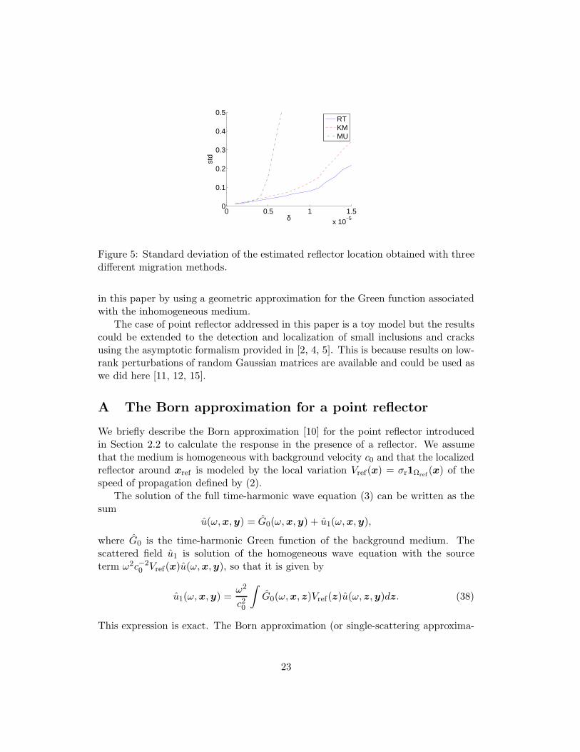
In Figure 5 the standard deviation in the reflector location is plotted versus thenoise level for the different imaging functionals. As predicted by the theory theMUSIC algorithm is not very robust and fails when δ > 5 10−5, or equivalentlyσc > 5 10−5 ∼ σref . The reverse-time imaging functional is more robust, and formoderate noise level the standard deviation is linear in δ. Indeed the reverse-timeimaging functional backpropagates not only the first singular vector, but all of them(weighted by their singular values), and since only the backpropagation of the sin-gular vector corresponding to the reflector gives a peak, while the backpropagationof the other singular vectors just gives noise, we can still observe a peak centered atthe reflector location even in the regime when the first singular vector is not the onecorresponding to the reflector. This is what is shown by the statistical argumentsdeveloped in the previous section.

We can also notice that reverse-time imaging performs slightly better than Kirch-hoff migration imaging. This is in agreement with the theory of the previous section

21

Figure 3: Imaging functionals in the absence of noise (left: reverse-time migration,center: Kirchhoff migration, right: MUSIC).

Figure 4: Imaging functionals in the presence of noise.

and can be noticed in the simulations carried out here because the array has verylarge aperture, so that the amplitudes of the Green functions in the vector g(x)are not constant. If the array has small aperture then the vectors g(x) (used inreverse-time migration) and d(x) (used in Kirchhoff migration) are very similar andthe difference between the two imaging functionals is small.

6 Conclusion

In this paper we have carefully studied detection tests based on the SVD of theresponse matrix or on weighted subspace migration by using recent tools of randommatrix theory and extreme value theory for Gaussian fields. In both cases we haveproved a form of optimality in that we have designed tests that are the most powerfulfor a given false alarm rate in the presence of additive noise. We have also provedthat reflector localization should be performed with reverse-time migration ratherthan any other form of weighted-subspace migration.

In this paper we have assumed that the background medium is homogeneous forsimplicity. It is possible to extend the results to the case in which the medium isslowly and smoothly varying. We would obtain the same results as the one derived

22

0 0.5 1 1.5

x 10−5

0

0.1

0.2

0.3

0.4

0.5

δst

d

RTKMMU

Figure 5: Standard deviation of the estimated reflector location obtained with threedifferent migration methods.

in this paper by using a geometric approximation for the Green function associatedwith the inhomogeneous medium.

The case of point reflector addressed in this paper is a toy model but the resultscould be extended to the detection and localization of small inclusions and cracksusing the asymptotic formalism provided in [2, 4, 5]. This is because results on low-rank perturbations of random Gaussian matrices are available and could be used aswe did here [11, 12, 15].

A The Born approximation for a point reflector

We briefly describe the Born approximation [10] for the point reflector introducedin Section 2.2 to calculate the response in the presence of a reflector. We assumethat the medium is homogeneous with background velocity c0 and that the localizedreflector around xref is modeled by the local variation Vref(x) = σr1Ωref

(x) of thespeed of propagation defined by (2).

The solution of the full time-harmonic wave equation (3) can be written as thesum

u(ω,x,y) = G0(ω,x,y) + u1(ω,x,y),

where G0 is the time-harmonic Green function of the background medium. Thescattered field u1 is solution of the homogeneous wave equation with the sourceterm ω2c−2

0 Vref(x)u(ω,x,y), so that it is given by

u1(ω,x,y) =ω2

c20

∫

G0(ω,x,z)Vref(z)u(ω,z,y)dz. (38)

This expression is exact. The Born approximation (or single-scattering approxima-

23

tion) consists in replacing u on the right side of (38) by the field G0, which gives:

u1(ω,x,y) ≃ ω2

c20

∫

G0(ω,x,z)Vref (z)G0(ω,z,y)dz.

This approximation is valid if the scattered field u1 is small compared to the incidentfield G0, which holds if the scattering amplitude σr is small. We also assume that thediameter lref of the scattering region Ωref is small compared to typical wavelength.We can then model the scatterer by a point scatterer and we can write the scatteredfield u1 in the form

u1(ω,x,y) =ω2

c20

σrl3refG0(ω,x,xref)G0(ω,xref ,y). (39)

B Some results on complex Gaussian random fields

Let Ω ⊂ Rd be a bounded domain and let (A(x))x∈Ω be a stationary NB smooth

? complex Gaussian random field with mean zero, i.e. a speckle pattern. The sta-tistical distribution of the random field is characterized by the covariance function:

C(x) = E[

A(x′)A(x′ + x)]

.

We assume here that C is real-valued. As we will see below, the relevant statisticalinformation about local and global maxima of the field is in the mean intensityI0 = C(0) = E[|A(x)|2] and in the matrix

Λ =(

E[

∂xjA(x)∂xl

A(x)])

j,l=1,...,d=

(

− ∂2xjxl

C(0))

j,l=1,...,d.

B.1 Local maxima of a complex Gaussian random field

We consider the intensity profile of the complex field:

I(x) = |A(x)|2,and we look for the statistical distribution of the local maxima of I(x).

Let us denote by MΩu the number of local maxima of I(x) in Ω with values larger

than u:

MΩu := Card

local maxima of (I(x))x∈Ω with values larger than u

.

We have [24] (which is an extension of Adler’s results [1] from the real to the complexcase):

E[MΩu ] =

|Ω|Vc

( u

I0

)d2 exp

(

− u

I0

)

(

1 + O(

( u

I0

)−1/2))

, for u ≫ I0,

where Vc is the hotspot volume defined in terms of the determinant of the Hessianof the covariance function:

Vc =I

d/20 πd/2

(detΛ)1/2.

24

B.2 Global maximum of a complex Gaussian random field

Let us denote by IΩmax the global maximum of the field over the domain Ω:

IΩmax = max

x∈Ω|A(x)|2.

When |Ω| ≫ Vc, the statistical distribution of IΩmax is of the form [24]

IΩmax = I0

[

ln( |Ω|

Vc

)

+d

2ln ln

( |Ω|Vc

)

− ln Z0

]

,

where Z0 follows an exponential distribution, or equivalently − ln Z0 follows a Gum-bel distribution with cumulative distribution function P(− ln Z0 ≤ x) = exp(−e−x).

B.3 The local shape of a local maxium

We first state a classical and fundamental lemma about Gaussian vectors.

Let us consider a Rn+p-valued random vector

(

y1

y2

)

with Gaussian statistics:

L((

y1

y2

))

∼ N((

y1

y2

)

,

(

R11 R12

R21 R22

))

.

The mean vectors y1 and y2 belong to Rn and R

p, respectively, the covariancematrix R11 has size n × n, R12 has size n × p, R21 = RT

12 has size p × n, and R22

has size p × p. Assume that the distribution of y2 is not degenerate, i.e., that R22

is invertible.Then, conditionally to y2, the distribution of y1 is Gaussian:

L(

y1|y2

)

∼ N(

y1 + R12R−122 (y2 − y2),R11 − R12R

−122 R21

)

.

Using this lemma one can show that, given that the random field A(x) has alocal maximum at x0 with amplitude A0 (with |A0| ≫

√I0), then we have locally

around x0:

A(x) ≃ A0

[C(x − x0)√I0

+ o(1)]

, [|A0| ≫√

I0].

References

[1] R. Adler, The Geometry of Random Fields, Wiley, New York, 1981.

[2] H. Ammari, P. Garapon, L. Guadarrama Bustos, and H. Kang, Transientanomaly imaging by the acoustic radiation force, J. Diff. Equat., to appear.

[3] H. Ammari, J. Garnier, H. Kang, W.-K. Park, and K. Solna, Imaging schemesfor perfectly conducting cracks, submitted.

25

[4] H. Ammari and H. Kang, Reconstruction of Small Inhomogeneities from Bound-

ary Measurements, Lecture Notes in Mathematics, Vol. 1846, Springer-Verlag,Berlin, 2004.

[5] H. Ammari, H. Kang, H. Lee, and W.K. Park, Asymptotic imaging of perfectlyconducting cracks, SIAM J. Sci. Comput. 32 (2010), 894–922.

[6] A. Aubry and A. Derode, Random matrix theory applied to acoustic backscat-tering and imaging in complex media, Phys. Rev. Lett. 102 (2009), 084301.

[7] N. Bleistein, J. Cohen, and J. S. Jr Stockwell, Mathematics of Multidimensional

Seismic Imaging, Migration, and Inversion, Springer, New York, 2001.

[8] L. Borcea, G. Papanicolaou, C. Tsogka, and J. Berryman, Imaging and timereversal in random media, Inverse Problems 18 (2002) 1247–1279.

[9] L. Borcea, G. Papanicolaou, and F. G. Vasquez, Edge illumination and imagingof extended reflectors, SIAM J. Imaging Sci. 1 (2008), 75–114.

[10] M. Born and E. Wolf, Principles of Optics, Academic Press, New York, 1970.

[11] M. Capitaine, C. Donati-Martin, and D. Feral, The largest eigenvalue of finiterank deformation of large Wigner matrices: convergence and nonuniversality ofthe fluctuations, Ann. Probab. 37 (2009), 1–47.

[12] M. Capitaine, C. Donati-Martin, and D. Feral, Central limit theorems for eigen-values of deformations of Wigner matrices, arXiv:0903.4740v1.

[13] G. Casella and R. L. Berger, Statistical Inference, Duxbury Press, Pacific Grove,2002.

[14] A. J. Devaney, Time reversal imaging of obscured targets from multistatic data,IEEE Trans. Antennas Propagat. 523 (2005), 1600–1610.

[15] D. Feral and S. Peche, The largest eigenvalue of rank one deformation of largeWigner matrices, Comm. Math. Phys. 272 (2007), 185-228.

[16] A. Gut, Probability: A Graduate Course, Springer-Verlag, New-York, 2005.

[17] H. Lev-Ari and A. J. Devaney, The time-reversal technique reinterpreted: sub-space based signal processing for multi-static target location, EEE Sensor Arrayand Multichannel Signal Processing Workshop, Cambridge, MA, March 2000,509–513.

[18] M. L. Mehta, Random Matrices, Academic Press, San Diego, 1991.

[19] L. Pastur, On the spectrum of random matrices, Teor. Math. Phys. 10 (1972),67–74.

26

[20] S. Peche, The largest eigenvalue of small rank perturbations of Hermitian ran-dom matrices, Probab. Theory Related Fields 134 (2006), 127–173.

[21] S. M. Popoff, G. Lerosey, R. Carminati, M. Fink, A. C. Boccara, and S. Gigan,Measuring the transmission matrix in optics: An approach to the study andcontrol of light propagation in disordered media, Phys. Rev. Lett. 104 (2010),100601.

[22] C. Prada, S. Manneville, D. Spolianski, and M. Fink, Decomposition of thetime reversal operator: detection and selective focusing on two scatterers, J.Acoust. Soc. Am. 99 (1996), 2067–2076.

[23] R. A. DeVore and G. Lorentz, Constructive Approximation, Springer-Verlag,Berlin, 1993.

[24] K. J. Worsley, Local maxima and the expected Euler characteristic of excursionsets of χ2, F , and t fields, Adv. in Appl. Probab. 26 (1994), 13–42.

27