AFPC

A STATIC COMPUTABLE GENERAL EQUILIBRIUM MODEL OF AGRICULTURAL AND FORESTRY

REGIONAL MARKETS (AFRM

Agricultural and Food Policy CenterTexas A&M University

September 2012

Department of Agricultural EconomicsTexas AgriLife ResearchTexas AgriLife Extension ServiceTexas A&M University

College Station, Texas 77843-2124Telephone: (979) 845-5913

Fax: (979) 845-3140

© 2012 by the Agricultural and Food Policy Center

Research Report 12-3Agricultural and Food Policy CenterDepartment of Agricultural Economics2124 TAMUCollege Station, TX 77843-2124Web site: www.afpc.tamu.edu

3US Grain Sorghum Trade Flows

Juan J. MongeHenry L. Bryant

Agricultural & Food Policy CenterDepartment of Agricultural Economics

Texas AgriLife ResearchTexas AgriLife Extension Service

Texas A&M University

AFPC Research Report 12-3

September 2012

College Station, Texas 77843-2124Telephone: 979.845.5913

Fax: 979.845.3140

A STATIC COMPUTABLE GENERAL EQUILIBRIUM MODEL OF AGRICULTURAL AND FORESTRY

REGIONAL MARKETS (AFRM

AFPCAgricultural and F ood Po licy Center

The Texa s A&M Univ ersity System

Contents

1 Introduction 3

2 Data 4

2.1 Value-added decomposition . . . . . . . . . . . . . . . . . . . . . . . . . . . . . . . . 52.2 Aggregation of activities and regions . . . . . . . . . . . . . . . . . . . . . . . . . . . 62.3 Land heterogeneity . . . . . . . . . . . . . . . . . . . . . . . . . . . . . . . . . . . . . 8

3 Model 11

4 Activities, production and factor markets 12

5 Land markets 13

6 Institutions 17

6.1 Households . . . . . . . . . . . . . . . . . . . . . . . . . . . . . . . . . . . . . . . . . 176.2 Government . . . . . . . . . . . . . . . . . . . . . . . . . . . . . . . . . . . . . . . . . 186.3 Enterprises . . . . . . . . . . . . . . . . . . . . . . . . . . . . . . . . . . . . . . . . . 206.4 Inventory . . . . . . . . . . . . . . . . . . . . . . . . . . . . . . . . . . . . . . . . . . 216.5 Investment . . . . . . . . . . . . . . . . . . . . . . . . . . . . . . . . . . . . . . . . . 21

7 Commodity markets 22

7.1 Domestic . . . . . . . . . . . . . . . . . . . . . . . . . . . . . . . . . . . . . . . . . . 227.2 Trade . . . . . . . . . . . . . . . . . . . . . . . . . . . . . . . . . . . . . . . . . . . . 24

8 Macroeconomic balances 25

8.1 Government balance . . . . . . . . . . . . . . . . . . . . . . . . . . . . . . . . . . . . 258.2 Inventory balance . . . . . . . . . . . . . . . . . . . . . . . . . . . . . . . . . . . . . . 258.3 Investment balance . . . . . . . . . . . . . . . . . . . . . . . . . . . . . . . . . . . . . 258.4 External balance . . . . . . . . . . . . . . . . . . . . . . . . . . . . . . . . . . . . . . 25

Appendix 29

2

1 Introduction

This report provides a detailed description of a static IMPLAN SAM-based regional computablegeneral equilibrium (CGE) model, �rst developed in Monge (2012), with special emphasis on themarket for agricultural land in any arbitrary state-level aggregation in the U.S. The CGE modelstructure described in this document is a hybrid between Lofgren et al. (2002) and Bryant et al.(2011). The model is especially well-suited to analyzing economic shocks a�ecting land allocationbetween agriculture and forestry. Monge (2012) applied the model to analyze the land-use changefrom agriculture to forestry motivated by a forest-based carbon sequestration policy funded by thegovernment.

In the literature, CGE models belong to a broader group of models known as sector optimizationmodels. The alternative models belonging to this broad group are input-output (IO) and partialequilibrium (PE) models. IO models are mainly based on economic IO tables and take into accountthe economic linkages between di�erent producing sectors and regions. However, when the substi-tution (transformation) of inputs (outputs) going (coming) into (out of) a demand (production)function is key among the objectives of any study, the assumed �xed elasticity of substitution (viz.,σ = 0) by IO models makes these a less robust alternative.

Besides IO models, the second class of models applied in regional studies are PE models. PEmodels concentrate on speci�c sectors of an economy considering the other sectors exogenous tothe model. Models such as FASOM and USMP have been extensively used to model land-usechange among the agriculture and forestry sectors (Adams et al., 1999; Alig et al., 1997, 1998;Environmental Protection Agency (EPA)., 2005; Lewandrowski et al., 2004). The main advantageof these models is the detailed disaggregation of the sectors under scrutiny, which facilitates apolicy-impact analysis. However, most PE models represent land through reduced-form supply,yield, and area response equations, and do not consider its demand side (Kretschmer and Peterson,2010). In other words, PE models do not consider an explicit market for land and, as a result,ignore the substitutability of land, which is key to all land-use change studies. Hence, the approachthat circumvents IO models' �xed-substitutability limitation and PE models' scope limitation isthe CGE modeling approach.

A CGE model is essentially a set of equations that explains the optimizing behavior of thedi�erent actors in an economy through �rst order conditions. CGE models typically solve a setof �rst-order conditions derived from utility and pro�t optimization theory. Among the key com-ponents considered in CGE models are the �exible substitution of inputs going into a behavioralfunction and the explicit market of factors of production such as capital, labor and land.1 Theinputs and outputs of the production and utility functions to be maximized are re�ected by theproduction and consumption values recorded in the Social Accounting Matrix (SAM) in a spe-ci�c year. All of these transactions re�ected in the SAM in a speci�c year are assumed to be inequilibrium.

The SAM is a record-keeping framework of the payments between economic actors in a speci�ceconomic region and its regional context (i.e. trade). The economic actors included in any genericSAM are: activities, commodities, institutions, production factors and trade. An activity representsan aggregated �rm in any speci�c sector in the economy that consumes and produces commodi-ties as inputs and outputs, respectively. The institutions are the households, enterprises and thegovernment. The production factors are capital, labor and, in the case of agriculture and forestry,land. Each of these institutions receives payments for o�ering factors of production (households)and for o�ering commodities and services (enterprises). The government is modeled as a passiveinstitution that collects taxes, receives transfers and distributes these back into the economy.

1CGE models also consider the �exible transformation of outputs coming from a behavioral function.

3

2 Data

The model re�ects the sectoral and regional aggregations built and imported from IMPLAN, withactivities, their respective commodities, basic factors of production (labor and capital), agriculturalland as a factor of production divided into Major Land Resource Areas (MLRA), nine householdcategories based on income levels, six federal and state government divisions, enterprises, invest-ment, inventory and two trade accounts: the rest of the U.S. and the rest of the world.

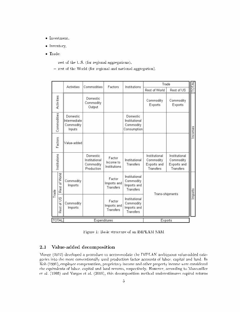
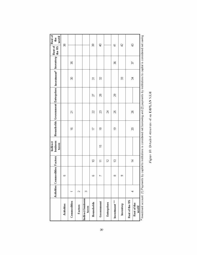
The SAMs used in this CGE model employ, as a primary source, data from the Impact Analysisfor Planning (IMPLAN) Version 3.0, re�ecting economic activity for 2008. The IMPLAN datasetcontains information for 440 activity sectors at the national, state and county level. Any genericSAM re�ects transactions among sectors of the economy as well as non-market transactions suchas transfers to and from the government. The basic structure of an IMPLAN SAM is shown in�gure 1. For a more detailed structure and the contents of every cell (transaction) please refer toMIG (1998) or �gure 10 in the appendix with its respective de�nitions in table 4.

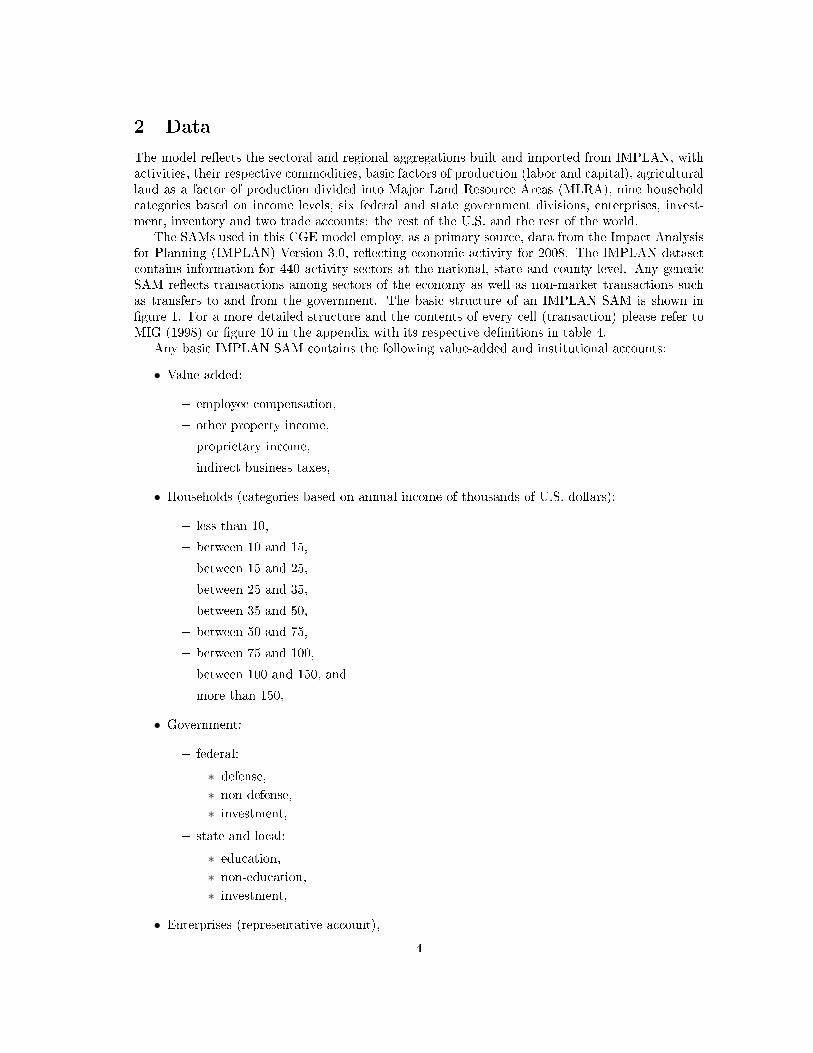
Any basic IMPLAN SAM contains the following value-added and institutional accounts:

• Value-added:

� employee compensation,

� other property income,

� proprietary income,

� indirect business taxes,

• Households (categories based on annual income of thousands of U.S. dollars):

� less than 10,

� between 10 and 15,

� between 15 and 25,

� between 25 and 35,

� between 35 and 50,

� between 50 and 75,

� between 75 and 100,

� between 100 and 150, and

� more than 150,

• Government:

� federal:

∗ defense,

∗ non-defense,

∗ investment,

� state and local:

∗ education,

∗ non-education,

∗ investment,

• Enterprises (representative account),

4

• Investment,

• Inventory,

• Trade:

� rest of the U.S. (for regional aggregations),

� rest of the World (for regional and national aggregation).

Figure 1: Basic structure of an IMPLAM SAM

2.1 Value-added decomposition

Monge (2012) developed a procedure to accommodate the IMPLAN ambiguous value-added cate-gories into the more conventionally used production factor accounts of labor, capital and land. InKoh (1991), employee compensation, proprietary income and other property income were consideredthe equivalents of labor, capital and land returns, respectively. However, according to Marcouilleret al. (1993) and Vargas et al. (2010), this decomposition method underestimates capital returns

5

and overestimates labor returns since proprietary income is de�ned as income from self employment.In other words, proprietary income includes a share of both capital and labor returns.

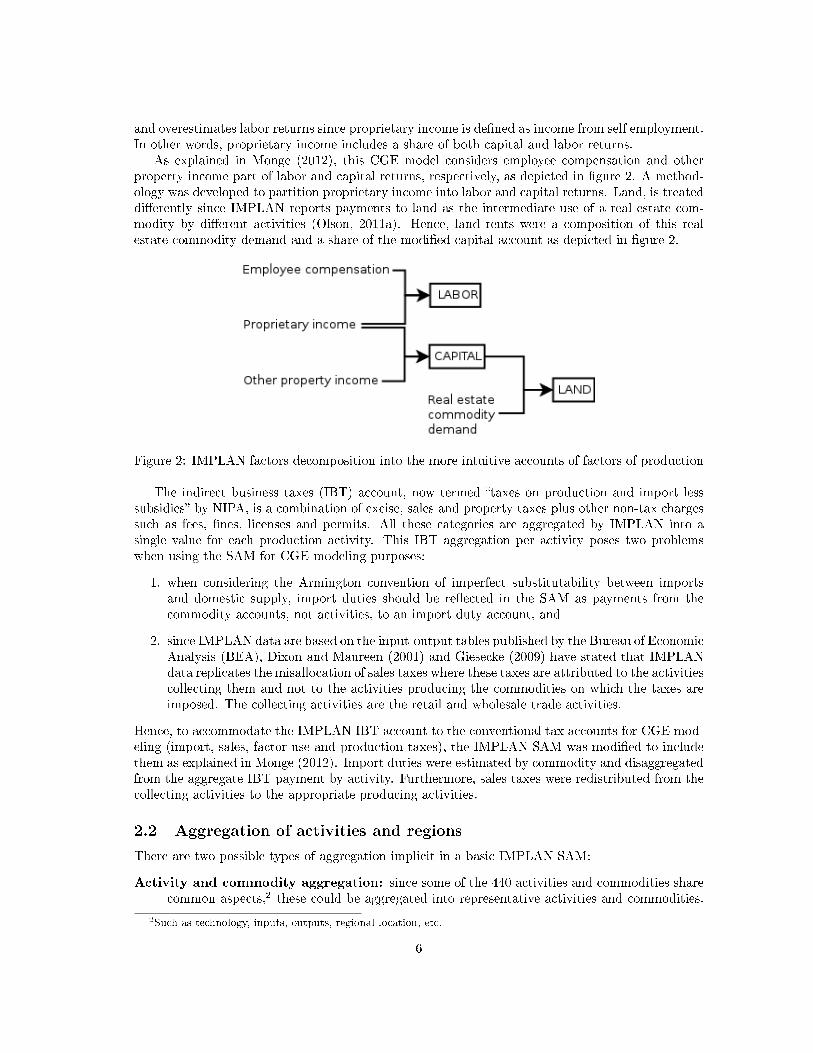
As explained in Monge (2012), this CGE model considers employee compensation and otherproperty income part of labor and capital returns, respectively, as depicted in �gure 2. A method-ology was developed to partition proprietary income into labor and capital returns. Land, is treateddi�erently since IMPLAN reports payments to land as the intermediate use of a real estate com-modity by di�erent activities (Olson, 2011a). Hence, land rents were a composition of this realestate commodity demand and a share of the modi�ed capital account as depicted in �gure 2.

Figure 2: IMPLAN factors decomposition into the more intuitive accounts of factors of production

The indirect business taxes (IBT) account, now termed �taxes on production and import lesssubsidies� by NIPA, is a combination of excise, sales and property taxes plus other non-tax chargessuch as fees, �nes, licenses and permits. All these categories are aggregated by IMPLAN into asingle value for each production activity. This IBT aggregation per activity poses two problemswhen using the SAM for CGE modeling purposes:

1. when considering the Armington convention of imperfect substitutability between importsand domestic supply, import duties should be re�ected in the SAM as payments from thecommodity accounts, not activities, to an import duty account, and

2. since IMPLAN data are based on the input-output tables published by the Bureau of EconomicAnalysis (BEA), Dixon and Maureen (2001) and Giesecke (2009) have stated that IMPLANdata replicates the misallocation of sales taxes where these taxes are attributed to the activitiescollecting them and not to the activities producing the commodities on which the taxes areimposed. The collecting activities are the retail and wholesale trade activities.

Hence, to accommodate the IMPLAN IBT account to the conventional tax accounts for CGE mod-eling (import, sales, factor-use and production taxes), the IMPLAN SAM was modi�ed to includethem as explained in Monge (2012). Import duties were estimated by commodity and disaggregatedfrom the aggregate IBT payment by activity. Furthermore, sales taxes were redistributed from thecollecting activities to the appropriate producing activities.

2.2 Aggregation of activities and regions

There are two possible types of aggregation implicit in a basic IMPLAN SAM:

Activity and commodity aggregation: since some of the 440 activities and commodities sharecommon aspects,2 these could be aggregated into representative activities and commodities.

2Such as technology, inputs, outputs, regional location, etc.

6

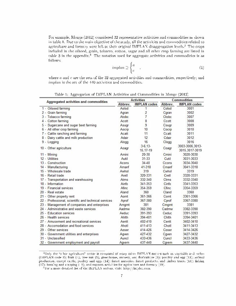
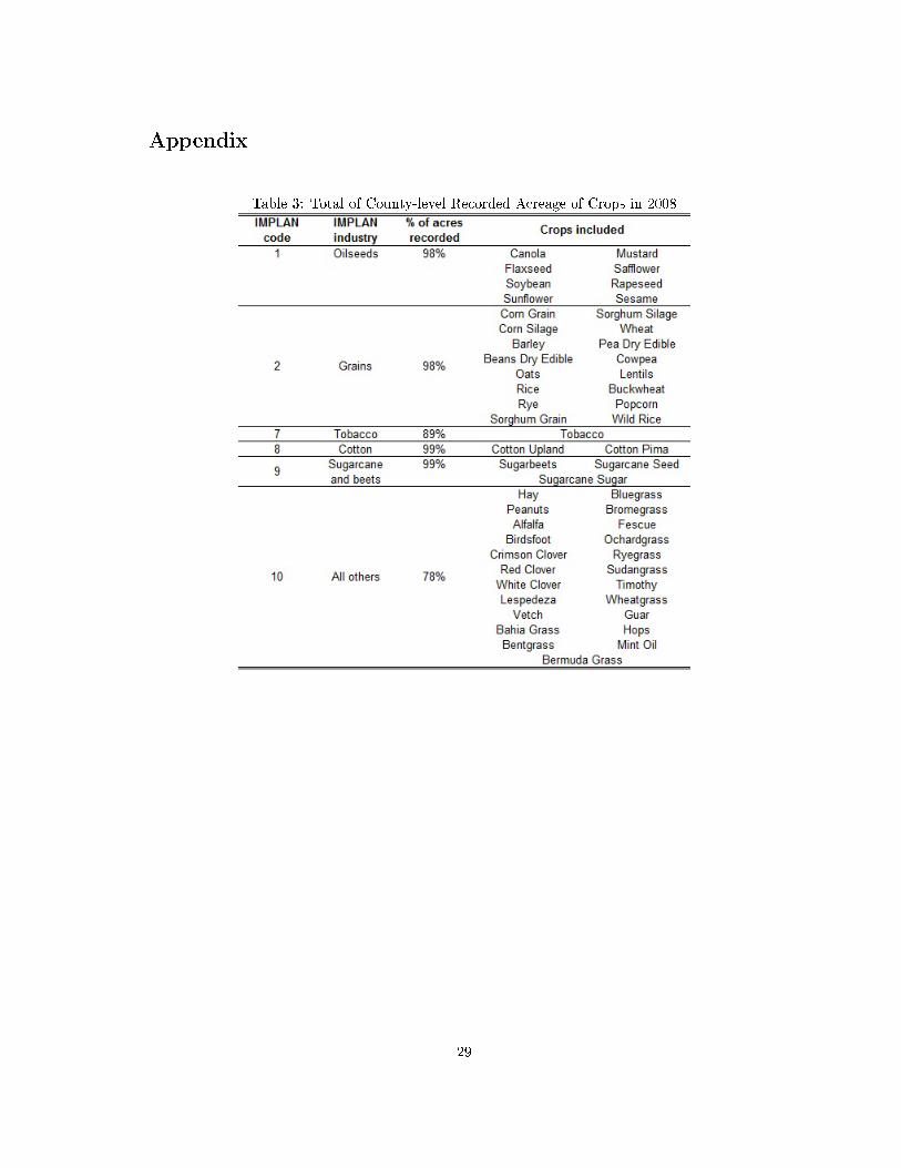
For example, Monge (2012) considered 32 representative activities and commodities as shownin table 1. Due to the main objective of the study, all the activities and commodities related toagriculture and forestry were left at their original IMPLAN disaggregation levels.3 The cropsincluded in the oilseed, grain, tobacco, cotton, sugar and all other crop farming are listed intable 3 in the appendix.4 The notation used for aggregate activities and commodities is asfollows:

implan ⊇

{a

c, (1)

where a and c are the sets of the 32 aggregated activities and commodities, respectively; andimplan is the set of the 440 activities and commodities.

Table 1: Aggregation of IMPLAN Activities and Commodities in Monge (2012)

3Only the �other agriculture� sector is composed of many other IMPLAN sectors such as vegetable and melon(IMPLAN code 3); fruit (4); tree nut (5); greenhouse, nursery, and �oriculture (6); poultry and egg (13); animalproduction, except cattle, poultry and eggs (14); forest nurseries, forest products, and timber tracts (15); �shing(17); hunting and trapping (18); and support activities for agriculture and forestry (19).

4For a more detailed list of the IMPLAN sectors, visit: http://implan.com.

7

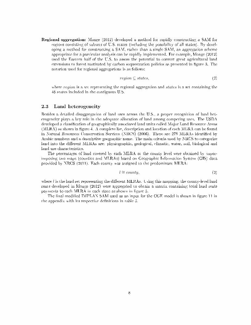
Regional aggregation: Monge (2012) developed a method for rapidly constructing a SAM forregions consisting of subsets of U.S. states (including the possibility of all states). By devel-oping a method for constructing a SAM, rather than a single SAM, an aggregation schemeappropriate for a particular analysis can be rapidly implemented. For example, Monge (2012)used the Eastern half of the U.S. to assess the potential to convert great agricultural landextensions to forest motivated by carbon sequestration policies as presented in �gure 3. Thenotation used for regional aggregations is as follows:

region ⊆ states, (2)

where region is a set representing the regional aggregation and states is a set containing the48 states included in the contiguous U.S.

2.3 Land heterogeneity

Besides a detailed disaggregation of land uses across the U.S., a proper recognition of land het-erogeneity plays a key role in the adequate allocation of land among competing uses. The USDAdeveloped a classi�cation of geographically associated land units called Major Land Resource Areas(MLRA) as shown in �gure 4. A complete list, description and location of each MLRA can be foundin Natural Resources Conservation Services (NRCS) (2006). There are 278 MLRAs identi�ed byArabic numbers and a descriptive geographic name. The main criteria used by NRCS to categorizeland into the di�erent MLRAs are: physiographic, geological, climatic, water, soil, biological andland use characteristics.

The percentages of land covered by each MLRA at the county level were obtained by super-imposing two maps (counties and MLRAs) based on Geographic Information System (GIS) dataprovided by NRCS (2011). Each county was assigned to the predominant MLRA:

l ∼= county, (3)

where l is the land set representing the di�erent MLRAs. Using this mapping, the county-level landrents developed in Monge (2012) were aggregated to obtain a matrix containing total land rentspayments to each MLRA in each state as shown in �gure 5.

The �nal modi�ed IMPLAN SAM used as an input for the CGE model is shown in �gure 11 inthe appendix with its respective de�nitions in table 5.

8

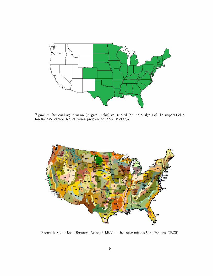
Figure 3: Regional aggregation (in green color) considered for the analysis of the impacts of aforest-based carbon sequestration program on land-use change

Figure 4: Major Land Resource Areas (MLRA) in the conterminous U.S. (Source: NRCS)

9

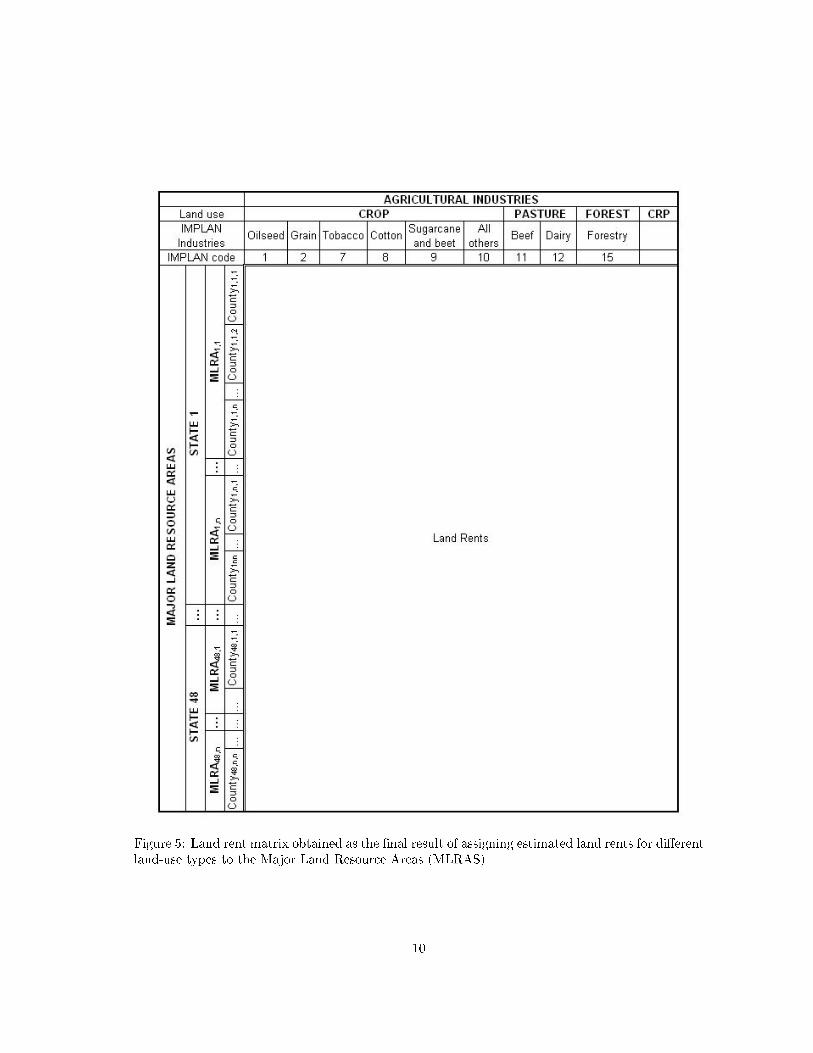
Figure 5: Land rent matrix obtained as the �nal result of assigning estimated land rents for di�erentland-use types to the Major Land Resource Areas (MLRAS)

10

3 Model

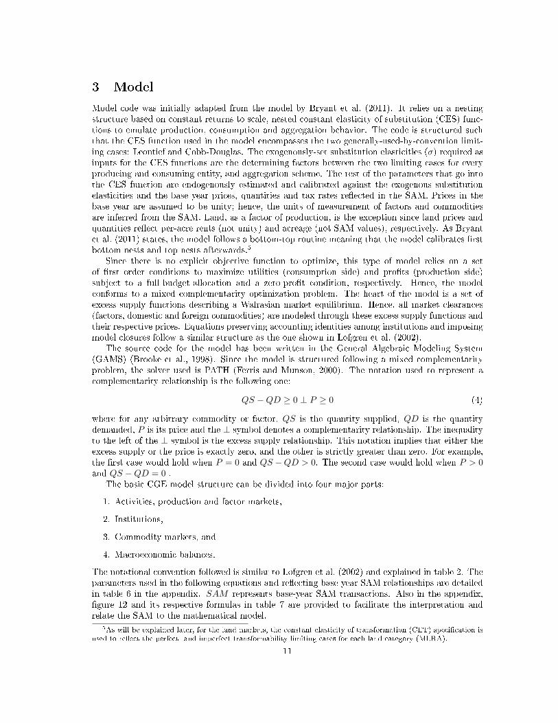
Model code was initially adapted from the model by Bryant et al. (2011). It relies on a nestingstructure based on constant returns to scale, nested constant elasticity of substitution (CES) func-tions to emulate production, consumption and aggregation behavior. The code is structured suchthat the CES function used in the model encompasses the two generally-used-by-convention limit-ing cases: Leontief and Cobb-Douglas. The exogenously-set substitution elasticities (σ) required asinputs for the CES functions are the determining factors between the two limiting cases for everyproducing and consuming entity, and aggregation scheme. The rest of the parameters that go intothe CES function are endogenously estimated and calibrated against the exogenous substitutionelasticities and the base year prices, quantities and tax rates re�ected in the SAM. Prices in thebase year are assumed to be unity; hence, the units of measurement of factors and commoditiesare inferred from the SAM. Land, as a factor of production, is the exception since land prices andquantities re�ect per-acre rents (not unity) and acreage (not SAM values), respectively. As Bryantet al. (2011) states, the model follows a bottom-top routine meaning that the model calibrates �rstbottom nests and top nests afterwards.5

Since there is no explicit objective function to optimize, this type of model relies on a setof �rst order conditions to maximize utilities (consumption side) and pro�ts (production side)subject to a full-budget-allocation and a zero-pro�t condition, respectively. Hence, the modelconforms to a mixed complementarity optimization problem. The heart of the model is a set ofexcess supply functions describing a Walrasian market equilibrium. Hence, all market clearances(factors, domestic and foreign commodities) are modeled through these excess supply functions andtheir respective prices. Equations preserving accounting identities among institutions and imposingmodel closures follow a similar structure as the one shown in Lofgren et al. (2002).

The source code for the model has been written in the General Algebraic Modeling System(GAMS) (Brooke et al., 1998). Since the model is structured following a mixed complementarityproblem, the solver used is PATH (Ferris and Munson, 2000). The notation used to represent acomplementarity relationship is the following one:

QS −QD ≥ 0 ⊥ P ≥ 0 (4)

where for any arbitrary commodity or factor, QS is the quantity supplied, QD is the quantitydemanded, P is its price and the ⊥ symbol denotes a complementarity relationship. The inequalityto the left of the ⊥ symbol is the excess supply relationship. This notation implies that either theexcess supply or the price is exactly zero, and the other is strictly greater than zero. For example,the �rst case would hold when P = 0 and QS −QD > 0. The second case would hold when P > 0and QS −QD = 0 .

The basic CGE model structure can be divided into four major parts:

1. Activities, production and factor markets,

2. Institutions,

3. Commodity markets, and

4. Macroeconomic balances.

The notational convention followed is similar to Lofgren et al. (2002) and explained in table 2. Theparameters used in the following equations and re�ecting base-year SAM relationships are detailedin table 6 in the appendix. SAM represents base-year SAM transactions. Also in the appendix,�gure 12 and its respective formulas in table 7 are provided to facilitate the interpretation andrelate the SAM to the mathematical model.

5As will be explained later, for the land markets, the constant elasticity of transformation (CET) speci�cation isused to re�ect the perfect- and imperfect-transformability limiting cases for each land category (MLRA).

11

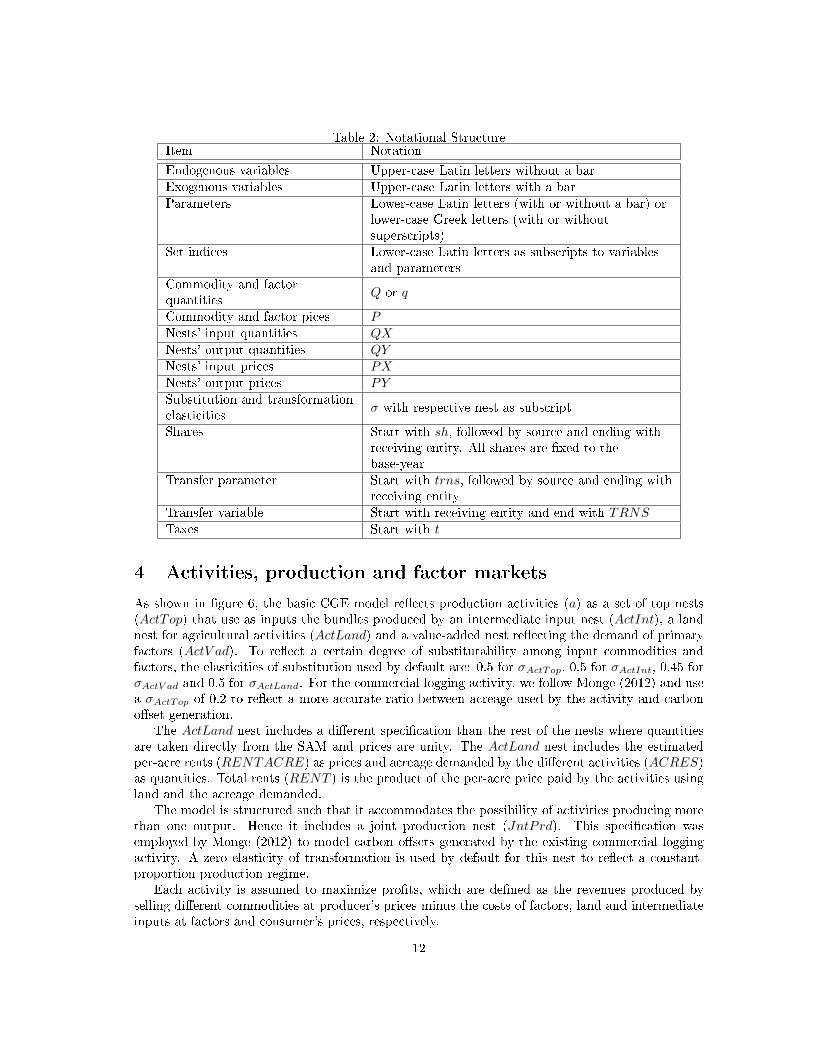
Table 2: Notational StructureItem Notation

Endogenous variables Upper-case Latin letters without a barExogenous variables Upper-case Latin letters with a barParameters Lower-case Latin letters (with or without a bar) or

lower-case Greek letters (with or withoutsuperscripts)

Set indices Lower-case Latin letters as subscripts to variablesand parameters

Commodity and factorquantities

Q or q

Commodity and factor pices PNests' input quantities QXNests' output quantities QYNests' input prices PXNests' output prices PYSubstitution and transformationelasticities

σ with respective nest as subscript

Shares Start with sh, followed by source and ending withreceiving entity. All shares are �xed to thebase-year

Transfer parameter Start with trns, followed by source and ending withreceiving entity

Transfer variable Start with receiving entity and end with TRNSTaxes Start with t

4 Activities, production and factor markets

As shown in �gure 6, the basic CGE model re�ects production activities (a) as a set of top nests(ActTop) that use as inputs the bundles produced by an intermediate input nest (ActInt), a landnest for agricultural activities (ActLand) and a value-added nest re�ecting the demand of primaryfactors (ActV ad). To re�ect a certain degree of substitutability among input commodities andfactors, the elasticities of substitution used by default are: 0.5 for σActTop, 0.5 for σActInt, 0.45 forσActV ad and 0.5 for σActLand. For the commercial logging activity, we follow Monge (2012) and usea σActTop of 0.2 to re�ect a more accurate ratio between acreage used by the activity and carbono�set generation.

The ActLand nest includes a di�erent speci�cation than the rest of the nests where quantitiesare taken directly from the SAM and prices are unity. The ActLand nest includes the estimatedper-acre rents (RENTACRE) as prices and acreage demanded by the di�erent activities (ACRES)as quantities. Total rents (RENT ) is the product of the per-acre price paid by the activities usingland and the acreage demanded.

The model is structured such that it accommodates the possibility of activities producing morethan one output. Hence it includes a joint production nest (JntPrd). This speci�cation wasemployed by Monge (2012) to model carbon o�sets generated by the existing commercial loggingactivity. A zero elasticity of transformation is used by default for this nest to re�ect a constant-proportion production regime.

Each activity is assumed to maximize pro�ts, which are de�ned as the revenues produced byselling di�erent commodities at producer's prices minus the costs of factors, land and intermediateinputs at factors and consumer's prices, respectively.

12

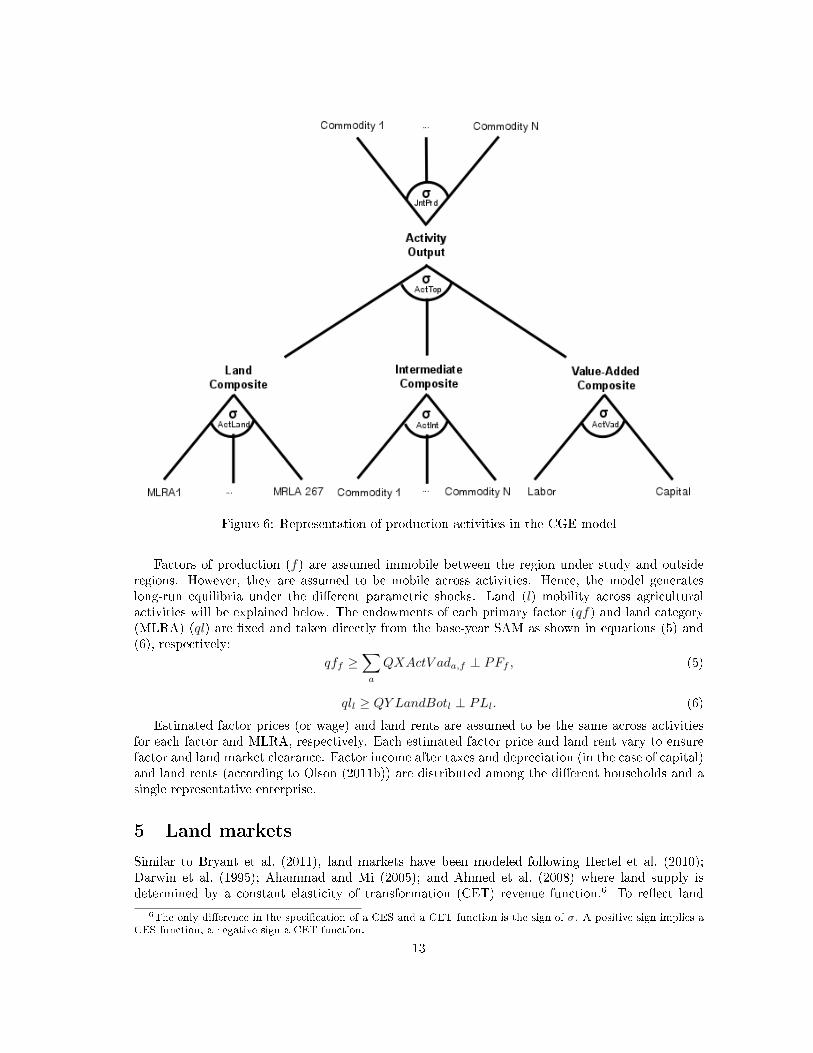
Figure 6: Representation of production activities in the CGE model

Factors of production (f) are assumed immobile between the region under study and outsideregions. However, they are assumed to be mobile across activities. Hence, the model generateslong-run equilibria under the di�erent parametric shocks. Land (l) mobility across agriculturalactivities will be explained below. The endowments of each primary factor (qf) and land category(MLRA) (ql) are �xed and taken directly from the base-year SAM as shown in equations (5) and(6), respectively:

qff ≥∑a

QXActV ada,f ⊥ PFf , (5)

qll ≥ QY LandBotl ⊥ PLl. (6)

Estimated factor prices (or wage) and land rents are assumed to be the same across activitiesfor each factor and MLRA, respectively. Each estimated factor price and land rent vary to ensurefactor and land market clearance. Factor income after taxes and depreciation (in the case of capital)and land rents (according to Olson (2011b)) are distributed among the di�erent households and asingle representative enterprise.

5 Land markets

Similar to Bryant et al. (2011), land markets have been modeled following Hertel et al. (2010);Darwin et al. (1995); Ahammad and Mi (2005); and Ahmed et al. (2008) where land supply isdetermined by a constant elasticity of transformation (CET) revenue function.6 To re�ect land

6The only di�erence in the speci�cation of a CES and a CET function is the sign of σ. A positive sign implies aCES function, a negative sign a CET function.

13

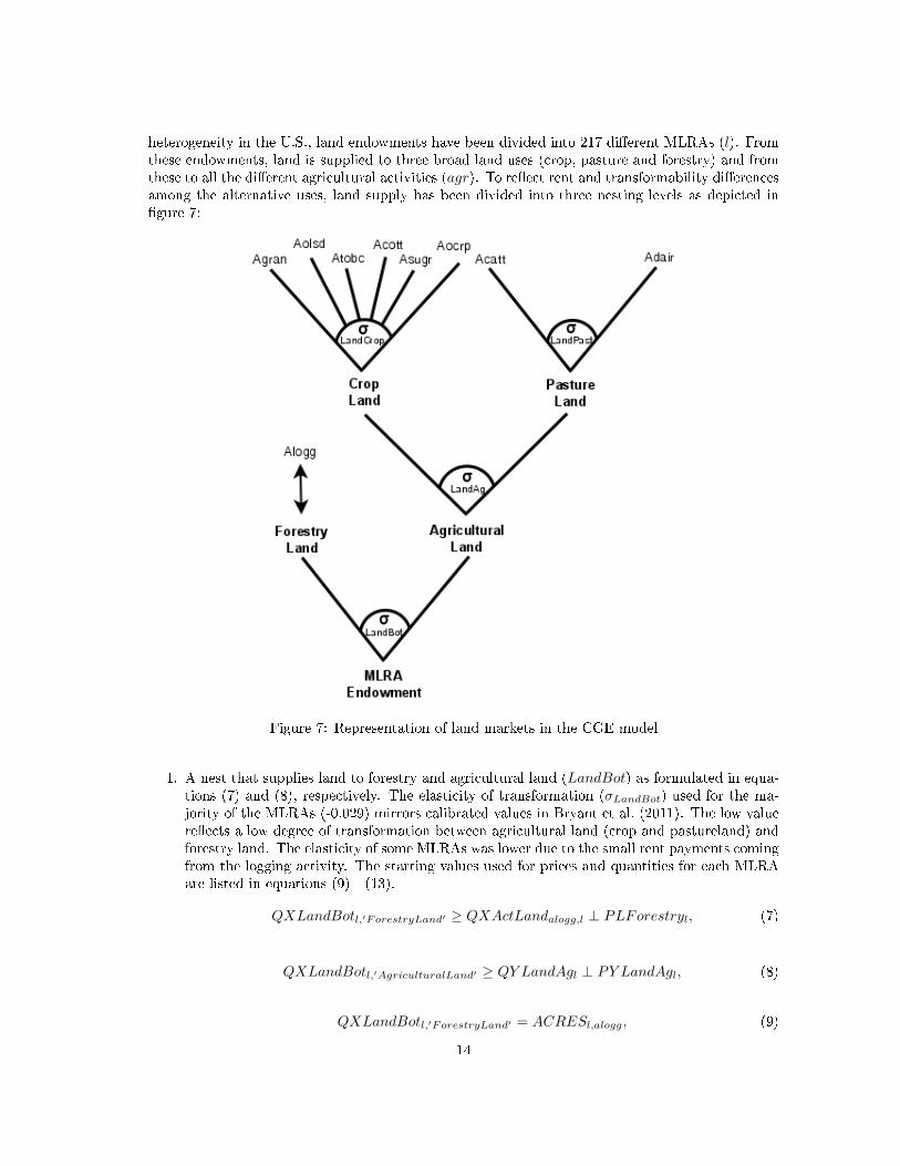
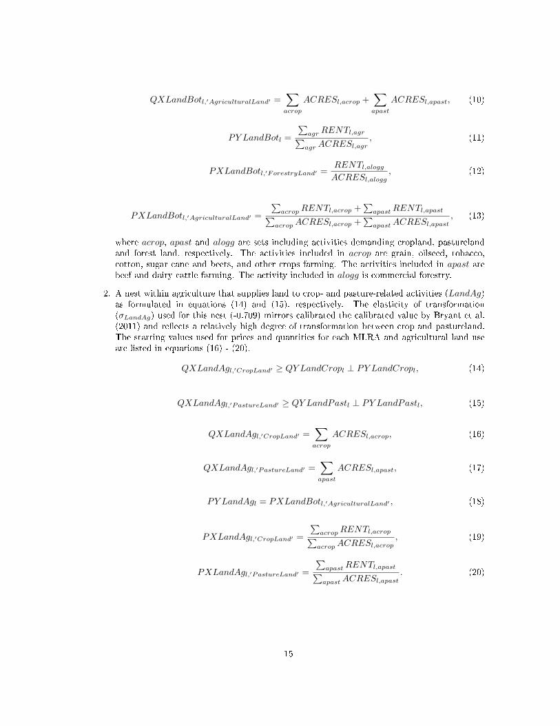
heterogeneity in the U.S., land endowments have been divided into 217 di�erent MLRAs (l). Fromthese endowments, land is supplied to three broad land uses (crop, pasture and forestry) and fromthese to all the di�erent agricultural activities (agr). To re�ect rent and transformability di�erencesamong the alternative uses, land supply has been divided into three nesting levels as depicted in�gure 7:

Figure 7: Representation of land markets in the CGE model

1. A nest that supplies land to forestry and agricultural land (LandBot) as formulated in equa-tions (7) and (8), respectively. The elasticity of transformation (σLandBot) used for the ma-jority of the MLRAs (-0.029) mirrors calibrated values in Bryant et al. (2011). The low valuere�ects a low degree of transformation between agricultural land (crop and pastureland) andforestry land. The elasticity of some MLRAs was lower due to the small rent payments comingfrom the logging activity. The starting values used for prices and quantities for each MLRAare listed in equations (9) - (13).

QXLandBotl,′ForestryLand′ ≥ QXActLandalogg,l ⊥ PLForestryl, (7)

QXLandBotl,′AgriculturalLand′ ≥ QY LandAgl ⊥ PY LandAgl, (8)

QXLandBotl,′ForestryLand′ = ACRESl,alogg, (9)

14

QXLandBotl,′AgriculturalLand′ =∑acrop

ACRESl,acrop +∑apast

ACRESl,apast, (10)

PY LandBotl =

∑agr RENTl,agr∑agr ACRESl,agr

, (11)

PXLandBotl,′ForestryLand′ =RENTl,aloggACRESl,alogg

, (12)

PXLandBotl,′AgriculturalLand′ =

∑acropRENTl,acrop +

∑apastRENTl,apast∑

acropACRESl,acrop +∑

apastACRESl,apast, (13)

where acrop, apast and alogg are sets including activities demanding cropland, pasturelandand forest land, respectively. The activities included in acrop are grain, oilseed, tobacco,cotton, sugar cane and beets, and other crops farming. The activities included in apast arebeef and dairy cattle farming. The activity included in alogg is commercial forestry.

2. A nest within agriculture that supplies land to crop- and pasture-related activities (LandAg)as formulated in equations (14) and (15), respectively. The elasticity of transformation(σLandAg) used for this nest (-0.709) mirrors calibrated the calibrated value by Bryant et al.(2011) and re�ects a relatively high degree of transformation between crop and pastureland.The starting values used for prices and quantities for each MLRA and agricultural land useare listed in equations (16) - (20).

QXLandAgl,′CropLand′ ≥ QY LandCropl ⊥ PY LandCropl, (14)

QXLandAgl,′PastureLand′ ≥ QY LandPastl ⊥ PY LandPastl, (15)

QXLandAgl,′CropLand′ =∑acrop

ACRESl,acrop, (16)

QXLandAgl,′PastureLand′ =∑apast

ACRESl,apast, (17)

PY LandAgl = PXLandBotl,′AgriculturalLand′ , (18)

PXLandAgl,′CropLand′ =

∑acropRENTl,acrop∑acropACRESl,acrop

, (19)

PXLandAgl,′PastureLand′ =

∑apastRENTl,apast∑apastACRESl,apast

. (20)

15

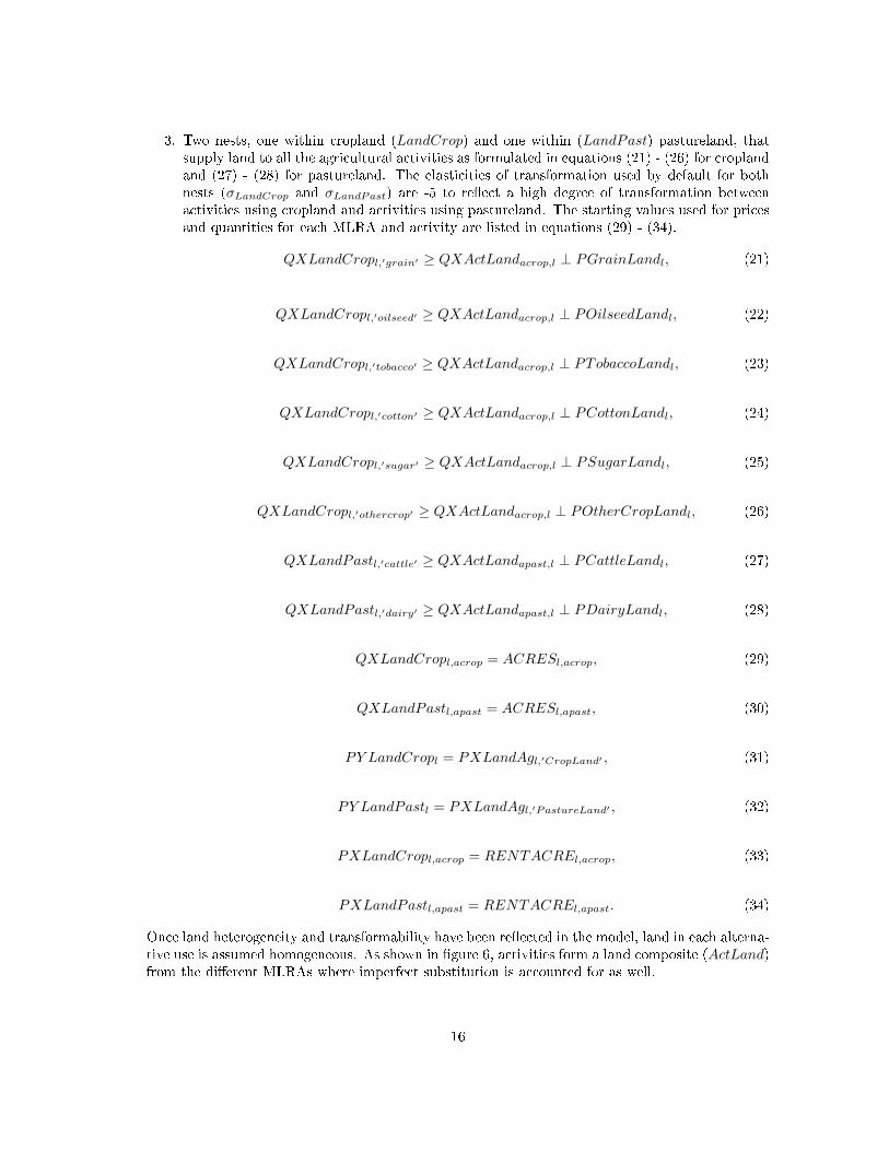
3. Two nests, one within cropland (LandCrop) and one within (LandPast) pastureland, thatsupply land to all the agricultural activities as formulated in equations (21) - (26) for croplandand (27) - (28) for pastureland. The elasticities of transformation used by default for bothnests (σLandCrop and σLandPast) are -5 to re�ect a high degree of transformation betweenactivities using cropland and activities using pastureland. The starting values used for pricesand quantities for each MLRA and activity are listed in equations (29) - (34).

QXLandCropl,′grain′ ≥ QXActLandacrop,l ⊥ PGrainLandl, (21)

QXLandCropl,′oilseed′ ≥ QXActLandacrop,l ⊥ POilseedLandl, (22)

QXLandCropl,′tobacco′ ≥ QXActLandacrop,l ⊥ PTobaccoLandl, (23)

QXLandCropl,′cotton′ ≥ QXActLandacrop,l ⊥ PCottonLandl, (24)

QXLandCropl,′sugar′ ≥ QXActLandacrop,l ⊥ PSugarLandl, (25)

QXLandCropl,′othercrop′ ≥ QXActLandacrop,l ⊥ POtherCropLandl, (26)

QXLandPastl,′cattle′ ≥ QXActLandapast,l ⊥ PCattleLandl, (27)

QXLandPastl,′dairy′ ≥ QXActLandapast,l ⊥ PDairyLandl, (28)

QXLandCropl,acrop = ACRESl,acrop, (29)

QXLandPastl,apast = ACRESl,apast, (30)

PY LandCropl = PXLandAgl,′CropLand′ , (31)

PY LandPastl = PXLandAgl,′PastureLand′ , (32)

PXLandCropl,acrop = RENTACREl,acrop, (33)

PXLandPastl,apast = RENTACREl,apast. (34)

Once land heterogeneity and transformability have been re�ected in the model, land in each alterna-tive use is assumed homogeneous. As shown in �gure 6, activities form a land composite (ActLand)from the di�erent MLRAs where imperfect substitution is accounted for as well.

16

6 Institutions

In the CGE model, institutions are represented by nine household categories based on incomelevels, six federal and state government divisions, enterprises, investment, inventory and two tradeaccounts. Following, the model's mathematical statements re�ecting each institution's income andexpenditure will be detailed and explained.

6.1 Households

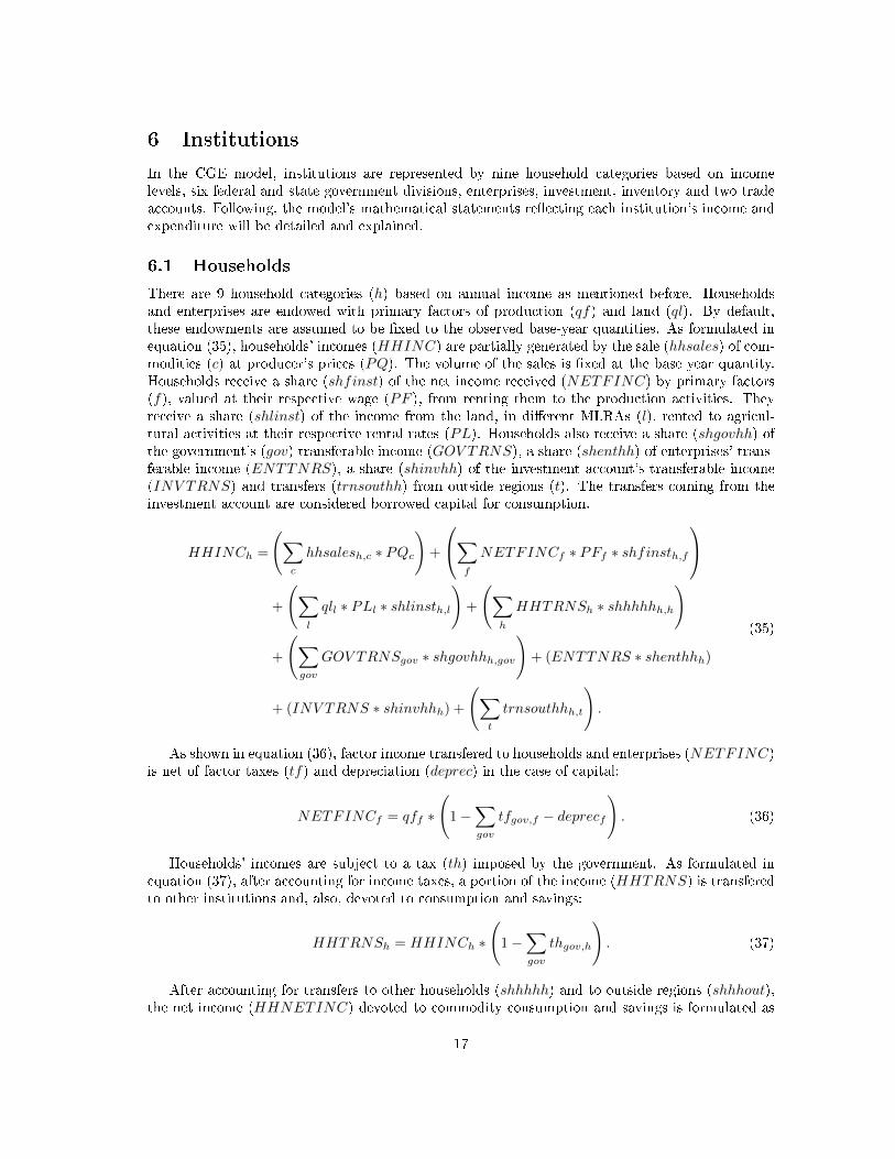
There are 9 household categories (h) based on annual income as mentioned before. Householdsand enterprises are endowed with primary factors of production (qf) and land (ql). By default,these endowments are assumed to be �xed to the observed base-year quantities. As formulated inequation (35), households' incomes (HHINC) are partially generated by the sale (hhsales) of com-modities (c) at producer's prices (PQ). The volume of the sales is �xed at the base year quantity.Households receive a share (shfinst) of the net income received (NETFINC) by primary factors(f), valued at their respective wage (PF ), from renting them to the production activities. Theyreceive a share (shlinst) of the income from the land, in di�erent MLRAs (l), rented to agricul-tural activities at their respective rental rates (PL). Households also receive a share (shgovhh) ofthe government's (gov) transferable income (GOV TRNS), a share (shenthh) of enterprises' trans-ferable income (ENTTNRS), a share (shinvhh) of the investment account's transferable income(INV TRNS) and transfers (trnsouthh) from outside regions (t). The transfers coming from theinvestment account are considered borrowed capital for consumption.

HHINCh =

(∑c

hhsalesh,c ∗ PQc

)+

∑f

NETFINCf ∗ PFf ∗ shfinsth,f

+

(∑l

qll ∗ PLl ∗ shlinsth,l

)+

(∑h

HHTRNSh ∗ shhhhhh,h

)

+

(∑gov

GOV TRNSgov ∗ shgovhhh,gov

)+ (ENTTNRS ∗ shenthhh)

+ (INV TRNS ∗ shinvhhh) +

(∑t

trnsouthhh,t

).

(35)

As shown in equation (36), factor income transfered to households and enterprises (NETFINC)is net of factor taxes (tf) and depreciation (deprec) in the case of capital:

NETFINCf = qff ∗

(1−

∑gov

tfgov,f − deprecf

). (36)

Households' incomes are subject to a tax (th) imposed by the government. As formulated inequation (37), after accounting for income taxes, a portion of the income (HHTRNS) is transferedto other institutions and, also, devoted to consumption and savings:

HHTRNSh = HHINCh ∗

(1−

∑gov

thgov,h

). (37)

After accounting for transfers to other households (shhhhh) and to outside regions (shhhout),the net income (HHNETINC) devoted to commodity consumption and savings is formulated as

17

in equation (38):

HHNETINCh = HHTRNSh ∗

(1−

∑h

shhhhhh,h −∑t

shhhoutt,h

). (38)

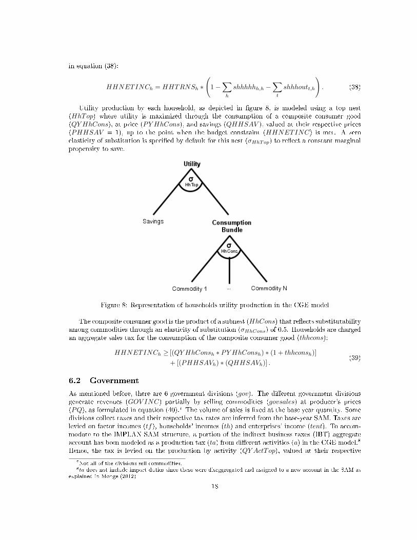
Utility production by each household, as depicted in �gure 8, is modeled using a top nest(HhTop) where utility is maximized through the consumption of a composite consumer good(QYHhCons), at price (PY HhCons), and savings (QHHSAV ), valued at their respective prices(PHHSAV = 1), up to the point when the budget constraint (HHNETINC) is met. A zeroelasticity of substitution is speci�ed by default for this nest (σHhTop) to re�ect a constant marginalpropensity to save.

Figure 8: Representation of households utility production in the CGE model

The composite consumer good is the product of a subnest (HhCons) that re�ects substitutabilityamong commodities through an elasticity of substitution (σHhCons) of 0.5. Households are chargedan aggregate sales tax for the consumption of the composite consumer good (thhcons):

HHNETINCh ≥ [(QYHhConsh ∗ PY HhConsh) ∗ (1 + thhconsh)]

+ [(PHHSAVh) ∗ (QHHSAVh)] .(39)

6.2 Government

As mentioned before, there are 6 government divisions (gov). The di�erent government divisionsgenerate revenues (GOV INC) partially by selling commodities (govsales) at producer's prices(PQ), as formulated in equation (40).7 The volume of sales is �xed at the base year quantity. Somedivisions collect taxes and their respective tax rates are inferred from the base-year SAM. Taxes arelevied on factor incomes (tf), households' incomes (th) and enterprises' income (tent). To accom-modate to the IMPLAN SAM structure, a portion of the indirect business taxes (IBT) aggregateaccount has been modeled as a production tax (ta) from di�erent activities (a) in the CGE model.8

Hence, the tax is levied on the production by activity (QY ActTop), valued at their respective

7Not all of the divisions sell commodities.8ta does not include import duties since these were disaggregated and assigned to a new account in the SAM as

explained in Monge (2012)

18

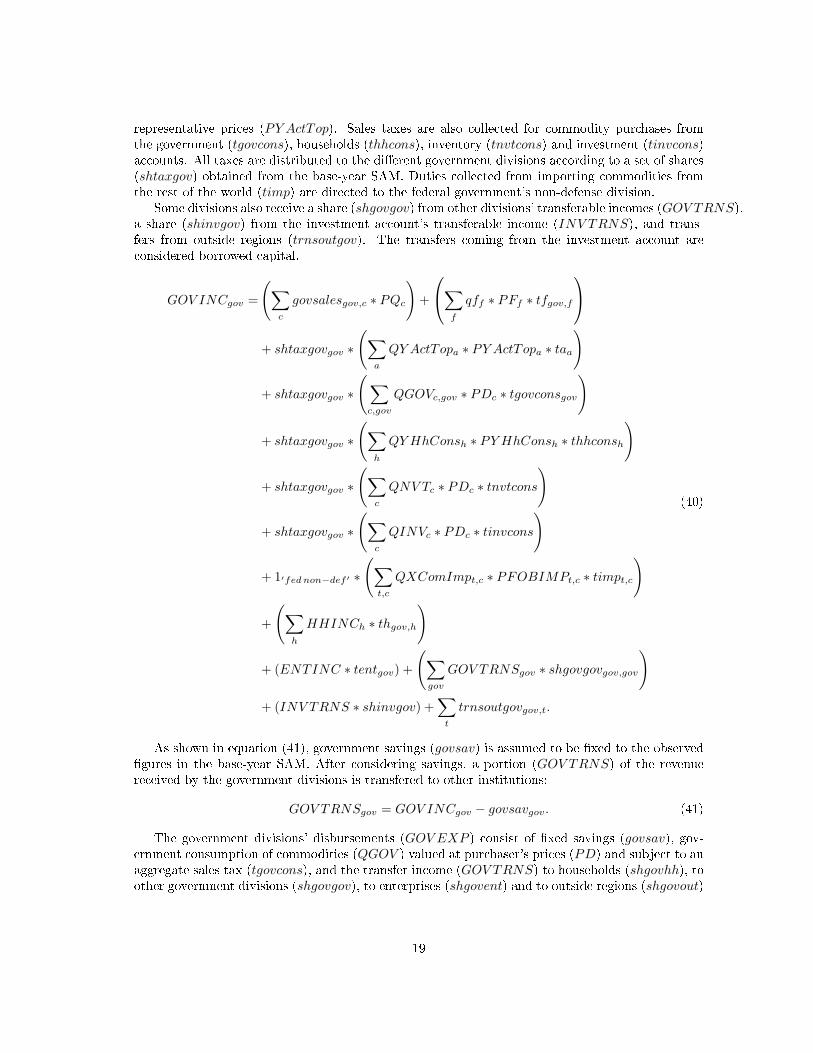
representative prices (PY ActTop). Sales taxes are also collected for commodity purchases fromthe government (tgovcons), households (thhcons), inventory (tnvtcons) and investment (tinvcons)accounts. All taxes are distributed to the di�erent government divisions according to a set of shares(shtaxgov) obtained from the base-year SAM. Duties collected from importing commodities fromthe rest of the world (timp) are directed to the federal government's non-defense division.

Some divisions also receive a share (shgovgov) from other divisions' transferable incomes (GOV TRNS),a share (shinvgov) from the investment account's transferable income (INV TRNS), and trans-fers from outside regions (trnsoutgov). The transfers coming from the investment account areconsidered borrowed capital.

GOV INCgov =

(∑c

govsalesgov,c ∗ PQc

)+

∑f

qff ∗ PFf ∗ tfgov,f

+ shtaxgovgov ∗

(∑a

QY ActTopa ∗ PY ActTopa ∗ taa

)

+ shtaxgovgov ∗

(∑c,gov

QGOVc,gov ∗ PDc ∗ tgovconsgov

)

+ shtaxgovgov ∗

(∑h

QYHhConsh ∗ PY HhConsh ∗ thhconsh

)

+ shtaxgovgov ∗

(∑c

QNV Tc ∗ PDc ∗ tnvtcons

)

+ shtaxgovgov ∗

(∑c

QINVc ∗ PDc ∗ tinvcons

)

+ 1′fed non−def ′ ∗

(∑t,c

QXComImpt,c ∗ PFOBIMPt,c ∗ timpt,c

)

+

(∑h

HHINCh ∗ thgov,h

)

+ (ENTINC ∗ tentgov) +

(∑gov

GOV TRNSgov ∗ shgovgovgov,gov

)+ (INV TRNS ∗ shinvgov) +

∑t

trnsoutgovgov,t.

(40)

As shown in equation (41), government savings (govsav) is assumed to be �xed to the observed�gures in the base-year SAM. After considering savings, a portion (GOV TRNS) of the revenuereceived by the government divisions is transfered to other institutions:

GOV TRNSgov = GOV INCgov − govsavgov. (41)

The government divisions' disbursements (GOV EXP ) consist of �xed savings (govsav), gov-ernment consumption of commodities (QGOV ) valued at purchaser's prices (PD) and subject to anaggregate sales tax (tgovcons), and the transfer income (GOV TRNS) to households (shgovhh), toother government divisions (shgovgov), to enterprises (shgovent) and to outside regions (shgovout)

19

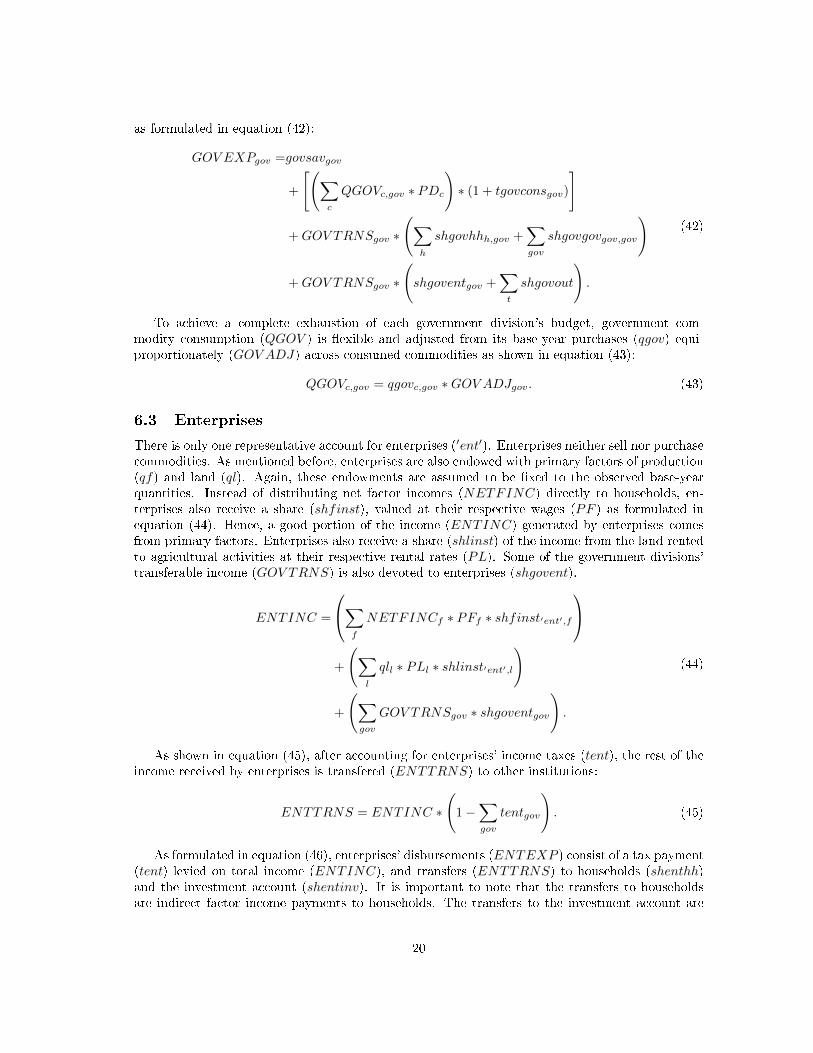
as formulated in equation (42):

GOV EXPgov =govsavgov

+

[(∑c

QGOVc,gov ∗ PDc

)∗ (1 + tgovconsgov)

]

+GOV TRNSgov ∗

(∑h

shgovhhh,gov +∑gov

shgovgovgov,gov

)

+GOV TRNSgov ∗

(shgoventgov +

∑t

shgovout

).

(42)

To achieve a complete exhaustion of each government division's budget, government com-modity consumption (QGOV ) is �exible and adjusted from its base-year purchases (qgov) equi-proportionately (GOV ADJ) across consumed commodities as shown in equation (43):

QGOVc,gov = qgovc,gov ∗GOV ADJgov. (43)

6.3 Enterprises

There is only one representative account for enterprises (′ent′). Enterprises neither sell nor purchasecommodities. As mentioned before, enterprises are also endowed with primary factors of production(qf) and land (ql). Again, these endowments are assumed to be �xed to the observed base-yearquantities. Instead of distributing net factor incomes (NETFINC) directly to households, en-terprises also receive a share (shfinst), valued at their respective wages (PF ) as formulated inequation (44). Hence, a good portion of the income (ENTINC) generated by enterprises comesfrom primary factors. Enterprises also receive a share (shlinst) of the income from the land rentedto agricultural activities at their respective rental rates (PL). Some of the government divisions'transferable income (GOV TRNS) is also devoted to enterprises (shgovent).

ENTINC =

∑f

NETFINCf ∗ PFf ∗ shfinst′ent′,f

+

(∑l

qll ∗ PLl ∗ shlinst′ent′,l

)

+

(∑gov

GOV TRNSgov ∗ shgoventgov

).

(44)

As shown in equation (45), after accounting for enterprises' income taxes (tent), the rest of theincome received by enterprises is transfered (ENTTRNS) to other institutions:

ENTTRNS = ENTINC ∗

(1−

∑gov

tentgov

). (45)

As formulated in equation (46), enterprises' disbursements (ENTEXP ) consist of a tax payment(tent) levied on total income (ENTINC), and transfers (ENTTRNS) to households (shenthh)and the investment account (shentinv). It is important to note that the transfers to householdsare indirect factor income payments to households. The transfers to the investment account are

20

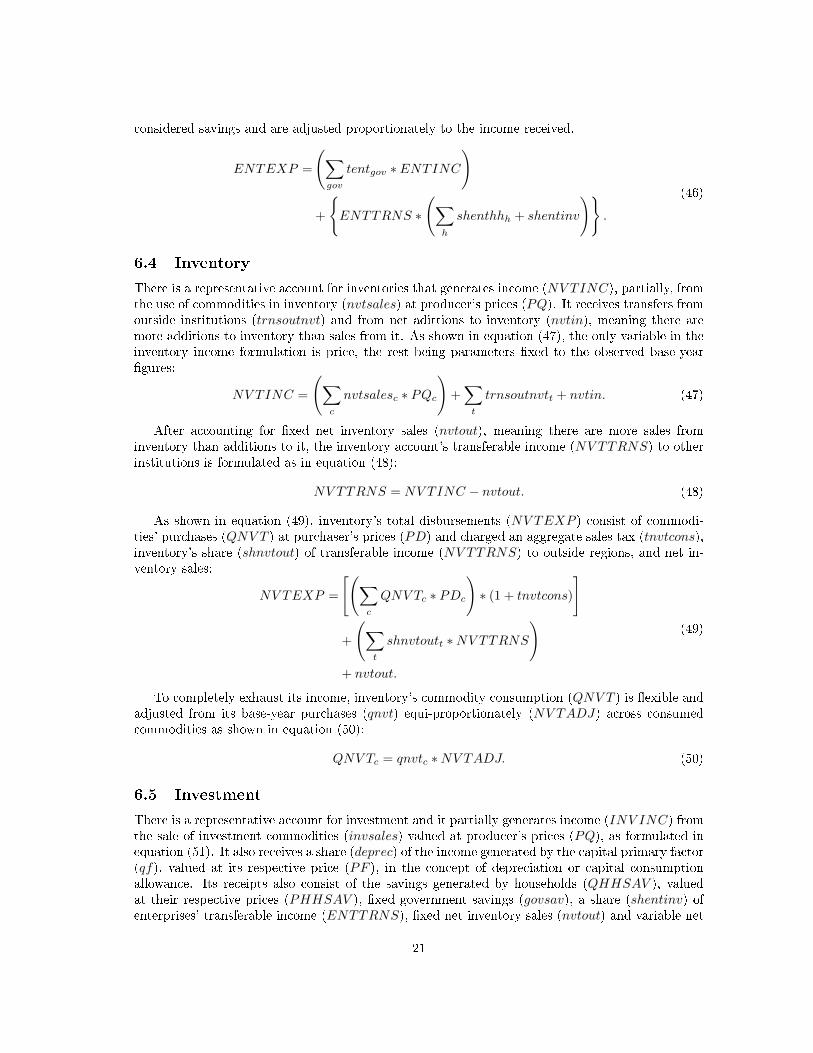
considered savings and are adjusted proportionately to the income received.

ENTEXP =

(∑gov

tentgov ∗ ENTINC

)

+

{ENTTRNS ∗

(∑h

shenthhh + shentinv

)}.

(46)

6.4 Inventory

There is a representative account for inventories that generates income (NV TINC), partially, fromthe use of commodities in inventory (nvtsales) at producer's prices (PQ). It receives transfers fromoutside institutions (trnsoutnvt) and from net adittions to inventory (nvtin), meaning there aremore additions to inventory than sales from it. As shown in equation (47), the only variable in theinventory income formulation is price, the rest being parameters �xed to the observed base-year�gures:

NV TINC =

(∑c

nvtsalesc ∗ PQc

)+∑t

trnsoutnvtt + nvtin. (47)

After accounting for �xed net inventory sales (nvtout), meaning there are more sales frominventory than additions to it, the inventory account's transferable income (NV TTRNS) to otherinstitutions is formulated as in equation (48):

NV TTRNS = NV TINC − nvtout. (48)

As shown in equation (49), inventory's total disbursements (NV TEXP ) consist of commodi-ties' purchases (QNV T ) at purchaser's prices (PD) and charged an aggregate sales tax (tnvtcons),inventory's share (shnvtout) of transferable income (NV TTRNS) to outside regions, and net in-ventory sales:

NV TEXP =

[(∑c

QNV Tc ∗ PDc

)∗ (1 + tnvtcons)

]

+

(∑t

shnvtoutt ∗NV TTRNS

)+ nvtout.

(49)

To completely exhaust its income, inventory's commodity consumption (QNV T ) is �exible andadjusted from its base-year purchases (qnvt) equi-proportionately (NV TADJ) across consumedcommodities as shown in equation (50):

QNV Tc = qnvtc ∗NV TADJ. (50)

6.5 Investment

There is a representative account for investment and it partially generates income (INV INC) fromthe sale of investment commodities (invsales) valued at producer's prices (PQ), as formulated inequation (51). It also receives a share (deprec) of the income generated by the capital primary factor(qf), valued at its respective price (PF ), in the concept of depreciation or capital consumptionallowance. Its receipts also consist of the savings generated by households (QHHSAV ), valuedat their respective prices (PHHSAV ), �xed government savings (govsav), a share (shentinv) ofenterprises' transferable income (ENTTRNS), �xed net inventory sales (nvtout) and variable net

21

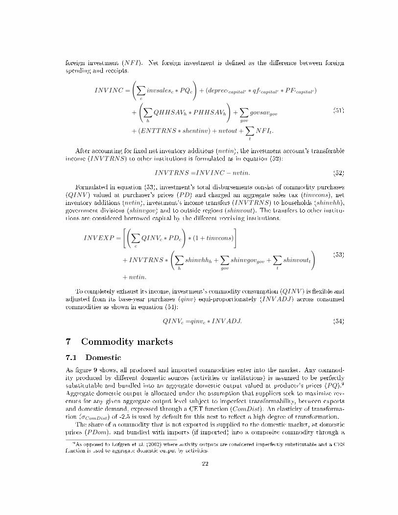
foreign investment (NFI). Net foreign investment is de�ned as the di�erence between foreignspending and receipts.

INV INC =

(∑c

invsalesc ∗ PQc

)+ (deprec′capital′ ∗ qf′capital′ ∗ PF′capital′)

+

(∑h

QHHSAVh ∗ PHHSAVh

)+∑gov

govsavgov

+ (ENTTRNS ∗ shentinv) + nvtout+∑t

NFIt.

(51)

After accounting for �xed net inventory additions (nvtin), the investment account's transferableincome (INV TRNS) to other institutions is formulated as in equation (52):

INV TRNS =INV INC − nvtin. (52)

Formulated in equation (53), investment's total disbursements consist of commodity purchases(QINV ) valued at purchaser's prices (PD) and charged an aggregate sales tax (tinvcons), netinventory additions (nvtin), investment's income transfers (INV TRNS) to households (shinvhh),government divisions (shinvgov) and to outside regions (shinvout). The transfers to other institu-tions are considered borrowed capital by the di�erent receiving institutions.

INV EXP =

[(∑c

QINVc ∗ PDc

)∗ (1 + tinvcons)

]

+ INV TRNS ∗

(∑h

shinvhhh +∑gov

shinvgovgov +∑t

shinvoutt

)+ nvtin.

(53)

To completely exhaust its income, investment's commodity consumption (QINV ) is �exible andadjusted from its base-year purchases (qinv) equi-proportionately (INV ADJ) across consumedcommodities as shown in equation (54):

QINVc =qinvc ∗ INV ADJ. (54)

7 Commodity markets

7.1 Domestic

As �gure 9 shows, all produced and imported commodities enter into the market. Any commod-ity produced by di�erent domestic sources (activities or institutions) is assumed to be perfectlysubstitutable and bundled into an aggregate domestic output valued at producer's prices (PQ).9

Aggregate domestic output is allocated under the assumption that suppliers seek to maximize rev-enues for any given aggregate output level subject to imperfect transformability, between exportsand domestic demand, expressed through a CET function (ComDist). An elasticity of transforma-tion (σComDist) of -2.5 is used by default for this nest to re�ect a high degree of transformation.

The share of a commodity that is not exported is supplied to the domestic market, at domesticprices (PDom), and bundled with imports (if imported) into a composite commodity through a

9As opposed to Lofgren et al. (2002) where activity outputs are considered imperfectly substitutable and a CESfunction is used to aggregate domestic output by activities.

22

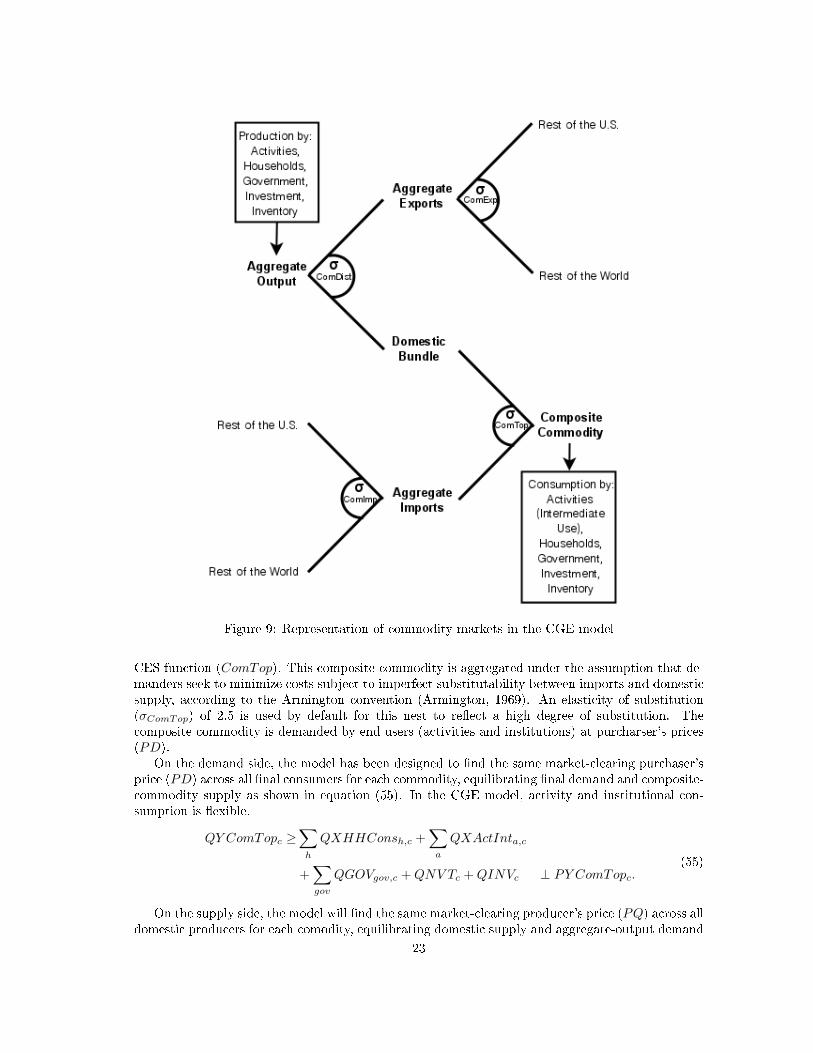
Figure 9: Representation of commodity markets in the CGE model

CES function (ComTop). This composite commodity is aggregated under the assumption that de-manders seek to minimize costs subject to imperfect substitutability between imports and domesticsupply, according to the Armington convention (Armington, 1969). An elasticity of substitution(σComTop) of 2.5 is used by default for this nest to re�ect a high degree of substitution. Thecomposite commodity is demanded by end users (activities and institutions) at purcharser's prices(PD).

On the demand side, the model has been designed to �nd the same market-clearing purchaser'sprice (PD) across all �nal consumers for each commodity, equilibrating �nal demand and composite-commodity supply as shown in equation (55). In the CGE model, activity and institutional con-sumption is �exible.

QY ComTopc ≥∑h

QXHHConsh,c +∑a

QXActInta,c

+∑gov

QGOVgov,c +QNV Tc +QINVc ⊥ PY ComTopc.(55)

On the supply side, the model will �nd the same market-clearing producer's price (PQ) across alldomestic producers for each comodity, equilibrating domestic supply and aggregate-output demand

23

as shown in equation (56). In the basic CGE model, only production by activities is �exible,institutional production is �xed to the base-year SAM.

QY ComDistc ≤∑a

QXJntPrda,c +∑h

hhsalesh,c

+∑

govsalesgov,c + nvtsalesc + invsalesc ⊥ PY ComDistc.(56)

In the modi�ed IMPLAN SAM, indirect business taxes include sales, production and factor-usetaxes. Due to the aggregated nature (and treatment as a production tax in this model) of theindirect business taxes account and to the non-existence of margin accounts (transportation andretail), all commodity transactions in an IMPLAN SAM are expressed in producer's prices. Inthe model, activities bear the entire burden of the taxes related to commodity production, exceptimport duties. Hence, producer's prices already include these taxes.10

7.2 Trade

Since the model is designed to accommodate large and small regional aggregations within theU.S., an exchange rate is not necessary due to the negligible e�ect that small aggregations wouldexert on world prices. Hence, traded commodities and institutional transfers are valued at thelocal currency (U.S. dollars). The model assumes the existence of a representative exporter andimporter for commodity-trading purposes. The exporter seeks to maximize revenues by sellingaggregate export commodities, to the rest of the U.S. and the rest of the world, and subject toimperfect transformability formulated through a CET function (ComExp) as depicted in �gure 9.An elasticity of transformation (σComExp) of -2.5 is used by default for this nest to re�ect a highdegree of transformation.

On the other side, the importer seeks to minimize costs by purchasing commodities, from therest of the U.S. and the rest of the world, and subject to imperfect substitutability expressed as aCES function (ComImp) as depicted in �gure 9. Commodities imported from the rest of the worldwere subject to import duties. An elasticity of substitution (σComImp) of 2.5 is used by default forthis nest to re�ect a high degree of substitution.

As shown in equation (57), export demands to outside regions are a function of base-yearSAM export quantities (qexp) and prices (pexp), prices charged by the representative exporter(PXComExp) and export demand elasticities (ε):

QEXPc,t = qexpc,t ∗ (1 + εc,t) ∗(PXComExpc,t − pexpc,t

pexpc,t

), (57)

where PXComExp is estimated as a shadow price of the excess supply equation for exports to eachdestination:

QXComExpc,t ≥ QEXPc,t ⊥ PXComExpc,t, (58)

where QXComExp is the quantity supplied by the ComExp nest.Import supplies from outside regions are a function of base-year SAM import quantities (qimp)

and prices (pimp), free-on-board (FOB) prices charged by the representative foreign exporter atthe foreign port (PFOBIMP ) and import supply elasticities (κ) as formulated in equation (59):

QIMPt,c = qimpt,c ∗ (1 + κt,c) ∗(PFOBIMPt,c − pimpt,c

pimpt,c

), (59)

10For any parametrical shock in the CGE model, the vector of market-clearing prices at a solution shows di�erencesbetween producer's prices (PQ) and purcharser's prices (PD). This di�erence is due to the e�ect of import andexport prices, respectively.

24

where the price paid by the representative importer (PIMP) is the FOB price after accounting forimport duties:

PIMPt,c = PFOBIMPt,c ∗ (1 + timpt,c,) , (60)

where PFOBIMP is estimated as a shadow price of the excess supply equation for imports fromeach source:

QIMPt,c ≥ QXComImpt,c ⊥ PFOBIMPt,c, (61)

where QXComImp is the quantity demanded by the ComImp nest.

8 Macroeconomic balances

8.1 Government balance

To completely exhaust the di�erent government divisions' budgets, the closure rule followed in theCGE structure is �exible government commodity consumption (QGOV ) and �xed savings (govsav).The adjustment factor (GOV ADJ) in equation (43) helps to achieve this balance and is paired toequation (62), following the syntax required by PATH to solve mixed complementarity problems.

GOV INCgov = GOV EXPgov. (62)

8.2 Inventory balance

To achieve a balance for the inventory account, the closure rule followed in the basic CGE structureis �exible inventory commodity consumption (QNV T ) and �xed net inventory deletions (nvtout).Again, the adjustment factor (NV TADJ) in equation (50) helps to achieve this balance and ispaired to equation (63).

NV TINC = NV TEXP. (63)

8.3 Investment balance

The same closure rule followed for the two previous institutions is applied to the investment account -investment commodity consumption (QINV ) is �exible. However, net foreign income (NFI) is also�exible in this case, as will be explained later. The adjustment factor (INV ADJ) in equation (54)helps to achieve this balance and is paired to equation (64).

INV INC = INV EXP. (64)

8.4 External balance

As previously mentioned, the model is designed to accommodate large and small regional ag-gregations within the U.S. Hence, an exchange rate variable is not necessary due to the negli-gible e�ect that small aggregations would exert on world prices. Thus, the closure variable forthe trade accounts is net foreign investment (NFI). As shown in equation (65), the left-hand-side variables re�ect receipts by the trade accounts consisting of commodity import quantities(QIMP ) valued at their respective import FOB prices (PFOBIMP ), and the di�erent transfersto outside regions by factors (shfout ∗ NETFINC), households (shhhout ∗ HHTRNS), gov-ernment divisions (shgovout ∗ GOV TRNS), investment (shinvout ∗ INV TRNS) and inventory(shnvtout ∗ NV TTRNS). The right-hand-side variables and parameters represent transfers fromoutside regions such as commodity export quantities (QEXP ) valued at their respective exportprices (PEXP ), foreign transfers to households (trnsouthh), government divisions (trnsoutgov),inventory (trnsoutnvt) and investment account or net foreign investment (NFI).

25

As previously listed in table 2, variables are represented by upper-case latin letters withouta bar and parameters with lower-case Latin letters without a bar. Hence, QIMP , PFOBIMP ,NETFINC, HHTRNS, GOV TRNS, INV TRNS, NV TTRNS, QEXP , PEXP and NFI areall �exible endogenous variables that adjust according to the model's closure rules such as equa-tion (65). The parameters shfout, shhhout, shgovout, shinvout, shnvtout, trnsouthh, trnsoutgov,trnsoutnvt are taken and �xed to the 2008 base year SAM.

It is important to mention that all transfers are variables that adjust according to the totalincome from the di�erent institutions. Prices and quantities of imported and exported commoditiesare variables. The expenditures from the di�erent institutions that are treated as transfers tooutside regions are estimated using shares from the base year SAM multiplied by the transferableinstitutional income variable. Transfers coming from outside regions to domestic institutions aretreated as �xed parameters and do not change from the baseline. Net foreign investment (NFI) isthe variable that is adjusted at last and the one that completes the model's closure.(∑

c

QIMPc,t ∗ PFOBIMPc,t

)

+

∑f

shfoutt,f ∗NETFINCf

+

(∑h

shhhoutt,h ∗HHTRNSh

)

+

(∑gov

shgovoutt,gov ∗GOV TRNSgov

)+(shinvoutt ∗ INV TRNS)+ (shnvtoutt ∗NV TTRNS)

=(∑c

QEXPc,t ∗ PEXPc,t

)+∑h

trnsouthhh,t

+∑gov

trnsoutgovgov,t

+ trnsoutnvtt

+NFIt.

(65)

26

References

Adams, D., Alig, R., McCarl, B., Callaway, J., and Winnett, S. (1999). Minimum cost strategiesfor sequestering carbon in forests. Land Economics, 75(3):360�374.

Ahammad, H. and Mi, R. (2005). Land use change modeling in GTEM: Accounting for forestsinks. In EMF22: Climate Change Control Scenarios, Standford University, California. AustralianBureau of Agricultural and Resource Economics.

Ahmed, S. A., Hertel, T. W., and Lubowski, R. (2008). Calibration of a land cover supply func-tion using transition probabilities. GTAP Research Memorandum 14, Center for Global TradeAnalysis, Purdue University.

Alig, R., Adams, D., and McCarl, B. (1998). Ecological and economic impacts of forest policies:Interactions across forestry and agriculture. Ecological Economics, 27:63�78.

Alig, R., Adams, D., McCarl, B., Callaway, J., and Winnett, S. (1997). Assessing e�ects of mit-igation strategies for global climate change with an intertemporal model of the U.S. forest andagriculture sectors. Environmental Resource Economics, 9:259�274.

Armington, P. S. (1969). A theory of demand for products distinguished by place of production.International Monetary Fund Sta� Papers 16, International Monetary Fund.

Brooke, A., Kendrick, D., Meeraus, A., and Raman, R. (1998). GAMS: A User's Guide. GAMSDevelopment Corporation, Washington, D.C.

Bryant, H. L., Campiche, J. L., and Lu, J. (2011). A static computable general equilibrium modelof world energy and agricultural markets (WEAM). AFPC Research Paper 11-1, Agriculturaland Food Policy Center, Texas A&M University, College Station, Texas.

Darwin, R., Tsigas, M., Lewandrowski, J., and Raneses, A. (1995). World agricutlure and climatechange: Economic adaptations. Agricultural Economic Report 703, Economic Research Service,U.S. Department of Agriculture, 341 Victory Drive. Herndon, VA, U.S.A.

Dixon, P. and Maureen, R. (2001). MONASH-USA: Creating a 1992 benchmark input-outputdatabase. Technical report, Centre of Policy Studies, Monash University. (Revised June 2002).

Environmental Protection Agency (EPA). (2005). Greenhouse gas mitigation potential in U.S.forestry and agriculture. Technical Report 430-R-05-006, O�ce of Atmospheric Programs, U.S.Environmental Protection Agency, Washington, D.C.

Ferris, M. C. and Munson, T. S. (2000). GAMS/PATH User Guide, Version 4.3.

Giesecke, J. A. (2009). Development of a large-scale single U.S. region CGE model using IMPLANdata: A Los Angeles county example with a productivity shock application. General Paper 187,Centre of Policy Studies, Monash University.

Hertel, T. W., Tyner, W. E., and Birur, D. K. (2010). The global impacts of biofuel mandates.The Energy Journal, 31(1):75�100.

Koh, Y.-K. (1991). Analysis of Oklahoma's Boom and Bust Economy. PhD thesis, Department ofAgricultural Economics, Oklahoma State University, Stillwater, OK.

Kretschmer, B. and Peterson, S. (2010). Integrating bioenergy into computable general equilibriummodels: A survey. Energy Economics, 32(3):673�686.

27

Lewandrowski, J., Peters, M., Jones, C., House, R., Sperow, M., Eve, M., and Paustian, K. (2004).Economics of sequestering carbon in the U.S. agricultural sector. Technical Bulletin 1909, Eco-nomic Research Service, U.S. Department of Agriculture, Washington, D.C.

Lofgren, H., Harris, R. L., Robinson, S., Thomas, M., and El-Said, M. (2002). A standard com-putable general equilibrium (CGE) model in GAMS. Microcomputers in Policy Research 5, In-ternational Food Policy Research Institute, 2033 K Street, N.W., Washington, D.C., 20006-1002,U.S.A.

Marcouiller, D. W., Schreiner, D. F., and Lewis, D. K. (1993). Constructing a social account-ing matrix to address distributive economic impacts of forest management. Regional SciencePerspectives, 23(2):60�90.

MIG, Inc. (1998). Elements of the social accounting matrix. MIG IMPLAN Technical ReportTR-98002, Minnesota IMPLAN Group, Inc.

Monge, J. J. (2012). Long-Run Implications of a Forest-Based Carbon Sequestration Policy on theUnited States Economy: A Computable General Equilibrium (CGE) Modeling Approach. PhDthesis, Texas A&M University, College Station, Texas.

Natural Resources Conservation Service (NRCS). (2006). Land resource regions and major landresource areas of the United States, the Caribbean, and the Paci�c Basin. USDA Handbook 296,U.S. Department of Agriculture.

Natural Resources Conservation Service (NRCS). (2011). Geospatial data gateway.http://datagateway.nrcs.usda.gov/ (accessed January 2011).

Olson, D. (2011a). Land rents in a CGE. Personal Communication. IMPLAN Sup-port Forum. http://implan.com/V4/index.php?option=com_kunena&func=view&catid=80&id-=8075&Itemid=35 (accessed February 2011).

Olson, D. (2011b). Real estate industry treated as a factor. Personal Communication. IMPLAN Sup-port Forum. http://implan.com/V4/index.php?option=com_kunena&func=view&catid=80&id-=8545&Itemid=35 (accessed April 2011).

Vargas, E., Schreiner, D., Tembo, G., and Marcouiller, D. (2010). Computable general equilibriummodeling for regional analysis. http://rri.wvu.edu/WebBook/Schreiner/contents.htm (accessedJuly 2010).

28

Appendix

Table 3: Total of County-level Recorded Acreage of Crops in 2008

29

Figure

10:Detailed

structure

ofanIM

PLANSAM

30

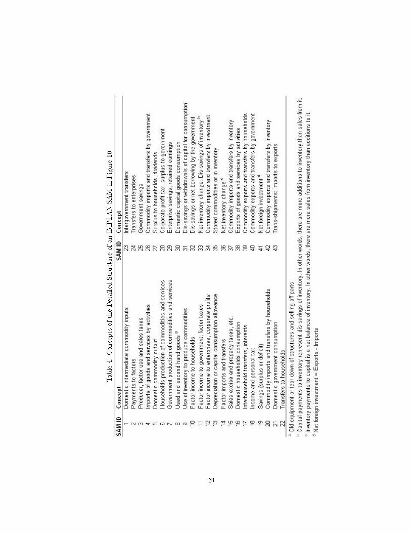
Table4:Concepts

oftheDetailed

Structure

ofanIM

PLANSAM

inFigure

10

31

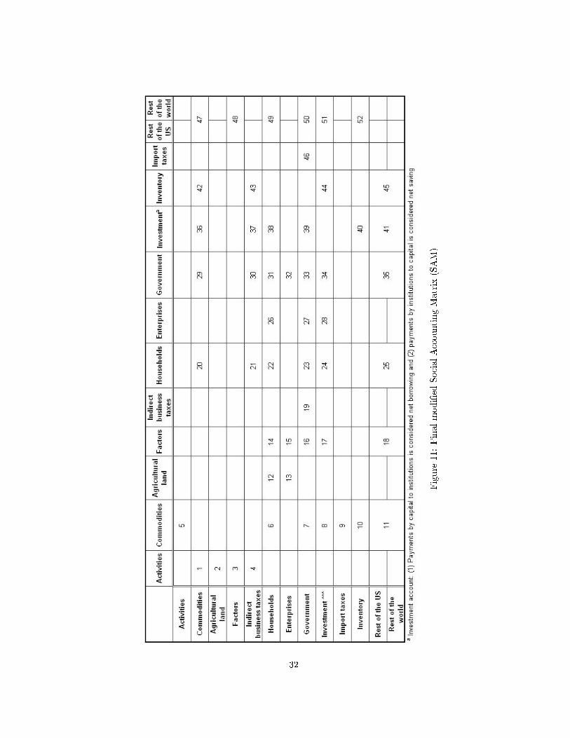
Figure

11:Finalmodi�ed

SocialAccountingMatrix

(SAM)

32

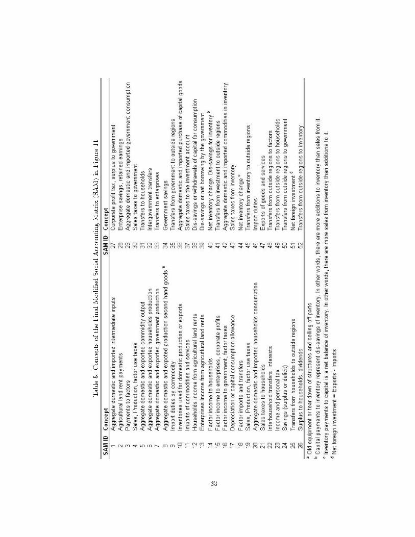
Table5:Concepts

oftheFinalModi�ed

SocialAccountingMatrix

(SAM)in

Figure

11

33

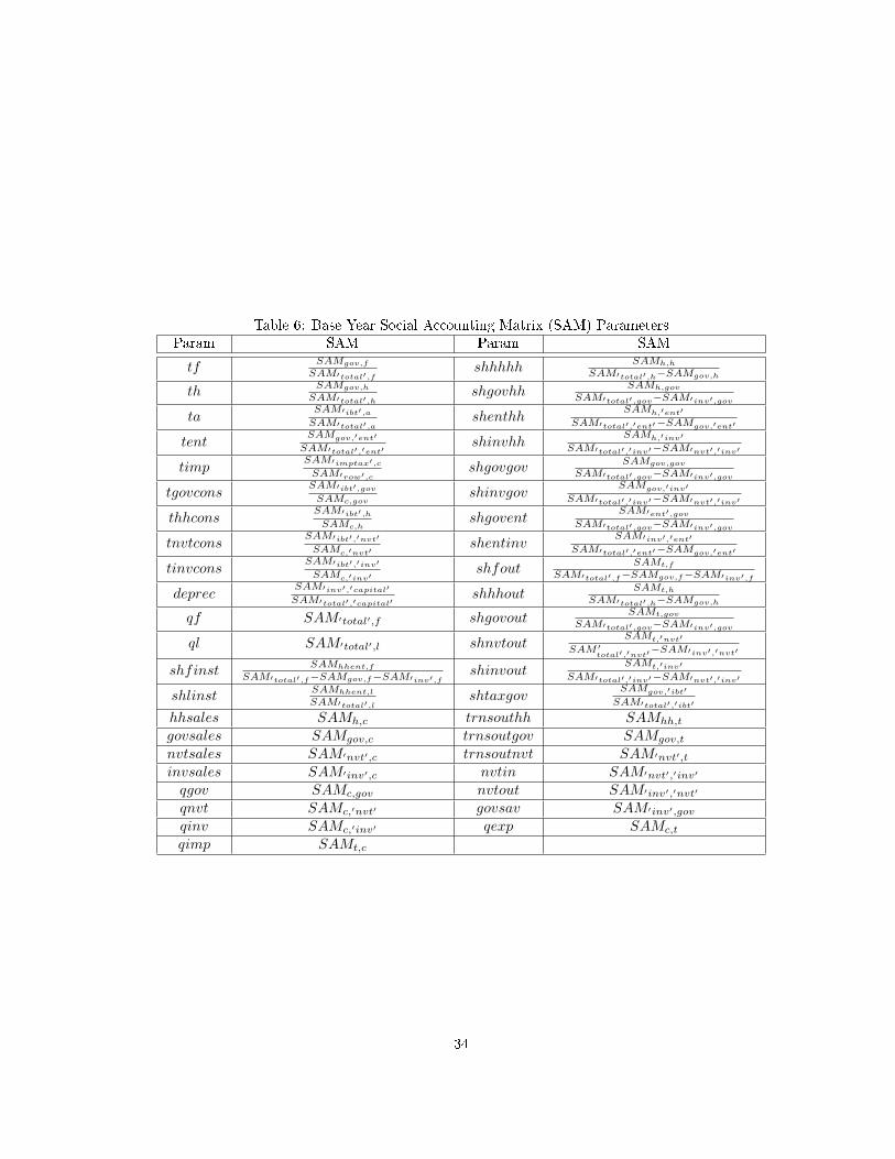
Table 6: Base Year Social Accounting Matrix (SAM) ParametersParam SAM Param SAM

tfSAMgov,f

SAM′total′,fshhhhh

SAMh,h

SAM′total′,h−SAMgov,h

thSAMgov,h

SAM′total′,hshgovhh

SAMh,gov

SAM′total′,gov−SAM′inv′,gov

taSAM′ibt′,aSAM′total′,a

shenthhSAMh,′ent′

SAM′total′,′ent′−SAMgov,′ent′

tentSAMgov,′ent′

SAM′total′,′ent′shinvhh

SAMh,′inv′

SAM′total′,′inv′−SAM′nvt′,′inv′

timpSAM′imptax′,cSAM′row′,c

shgovgovSAMgov,gov

SAM′total′,gov−SAM′inv′,gov

tgovconsSAM′ibt′,govSAMc,gov

shinvgovSAMgov,′inv′

SAM′total′,′inv′−SAM′nvt′,′inv′

thhconsSAM′ibt′,hSAMc,h

shgoventSAM′ent′,gov

SAM′total′,gov−SAM′inv′,gov

tnvtconsSAM′ibt′,′nvt′

SAMc,′nvt′shentinv

SAM′inv′,′ent′

SAM′total′,′ent′−SAMgov,′ent′

tinvconsSAM′ibt′,′inv′

SAMc,′inv′shfout

SAMt,f

SAM′total′,f−SAMgov,f−SAM′inv′,f

deprecSAM′inv′,′capital′

SAM′total′,′capital′shhhout

SAMt,h

SAM′total′,h−SAMgov,h

qf SAM′total′,f shgovoutSAMt,gov

SAM′total′,gov−SAM′inv′,gov

ql SAM′total′,l shnvtoutSAMt,′nvt′

SAM ′total′,′nvt′−SAM′inv′,′nvt′

shfinstSAMhhent,f

SAM′total′,f−SAMgov,f−SAM′inv′,fshinvout

SAMt,′inv′

SAM′total′,′inv′−SAM′nvt′,′inv′

shlinstSAMhhent,l

SAM′total′,lshtaxgov

SAMgov,′ibt′

SAM′total′,′ibt′

hhsales SAMh,c trnsouthh SAMhh,t

govsales SAMgov,c trnsoutgov SAMgov,t

nvtsales SAM′nvt′,c trnsoutnvt SAM′nvt′,t

invsales SAM′inv′,c nvtin SAM′nvt′,′inv′

qgov SAMc,gov nvtout SAM′inv′,′nvt′

qnvt SAMc,′nvt′ govsav SAM′inv′,gov

qinv SAMc,′inv′ qexp SAMc,t

qimp SAMt,c

34

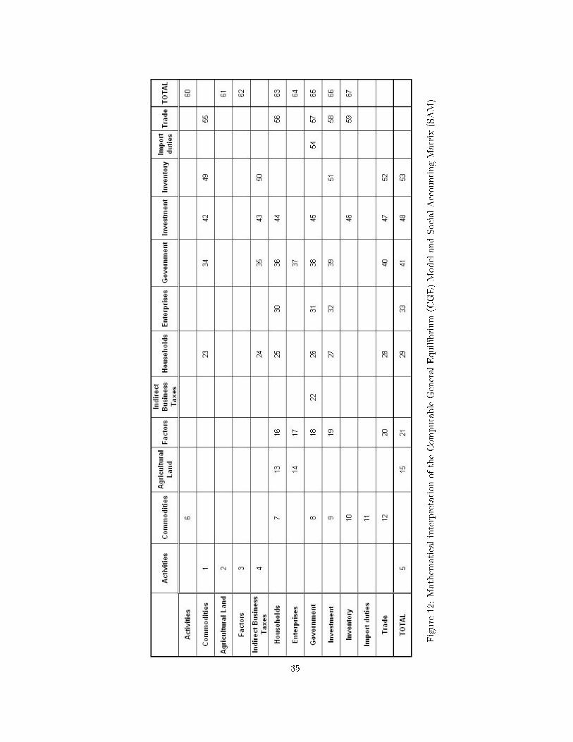
Figure

12:Mathem

aticalinterpretationoftheComputableGeneralEquilibrium

(CGE)ModelandSocialAccountingMatrix

(SAM)

35

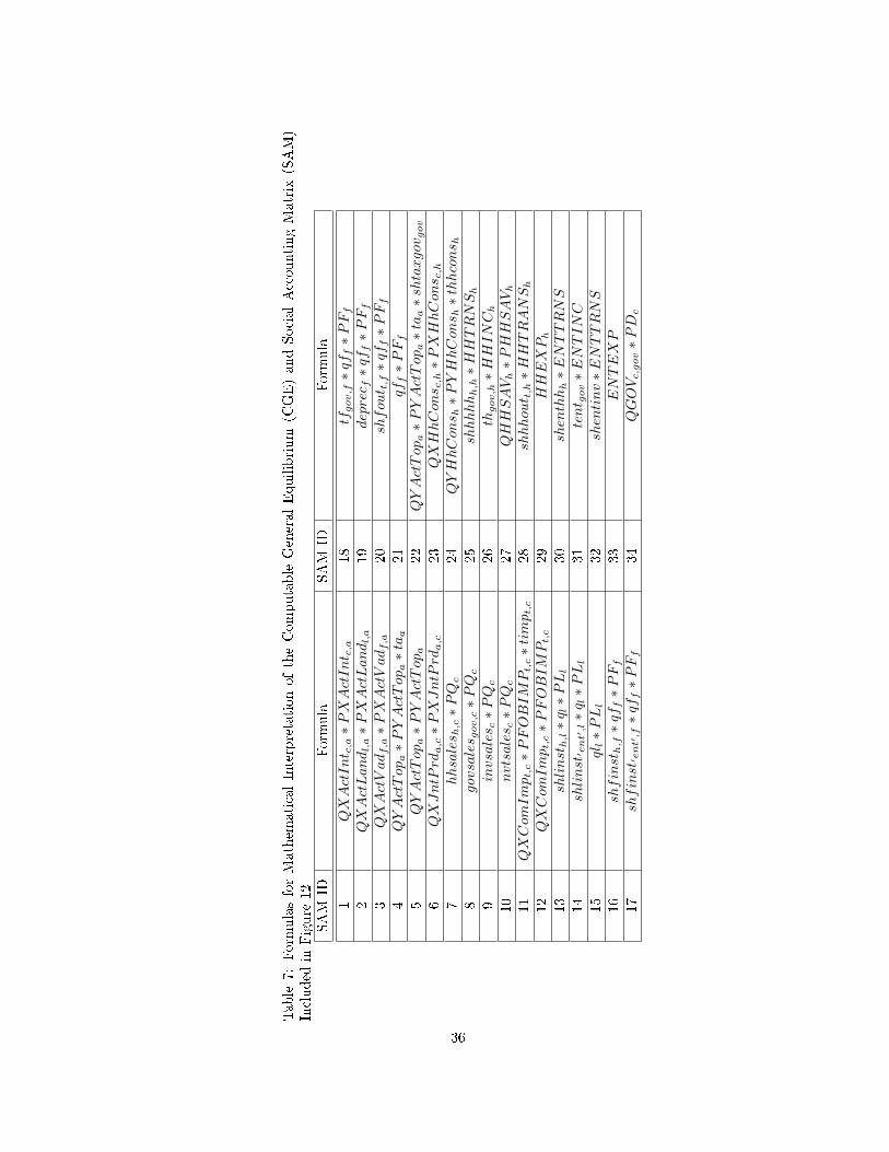
Table

7:Form

ulasforMathem

aticalInterpretationoftheComputable

GeneralEquilibrium

(CGE)andSocialAccountingMatrix

(SAM)

Included

inFigure

12

SAM

IDForm

ula

SAM

IDForm

ula

1QXActInt c

,a∗PXActInt c

,a18

tfgov,f∗qf

f∗PFf

2QXActLandl,a∗PXActLandl,a

19

deprec f∗qf

f∗PFf

3QXActVadf,a∗PXActVadf,a

20

shfout t,f∗qf

f∗PFf

4QYActTop

a∗PYActTop

a∗ta

a21

qff∗PFf

5QYActTop

a∗PYActTop

a22

QYActTop

a∗PYActTop

a∗ta

a∗shtaxgov

gov

6QXJntPrd

a,c∗PXJntPrd

a,c

23

QXHhCons c

,h∗PXHhCons c

,h

7hhsales h

,c∗PQ

c24

QYHhCons h∗PYHhCons h∗thhcons h

8govsales g

ov,c∗PQ

c25

shhhhhh,h∗HHTRNSh

9invsales c∗PQ

c26

thgov,h∗HHINC

h

10

nvtsales c∗PQ

c27

QHHSAVh∗PHHSAVh

11

QXCom

Impt,c∗PFOBIMPt,c∗timpt,c

28

shhhout t,h∗HHTRANSh

12

QXCom

Impt,c∗PFOBIMPt,c

29

HHEXPh

13

shlinst

h,l∗q l∗PLl

30

shenthhh∗ENTTRNS

14

shlinst

′ ent′,l∗q l∗PLl

31

tent g

ov∗ENTINC

15

qll∗PLl

32

shentinv∗ENTTRNS

16

shfinst

h,f∗qf

f∗PFf

33

ENTEXP

17

shfinst

′ ent′,f∗qf

f∗PFf

34

QGOVc,gov∗PD

c

36

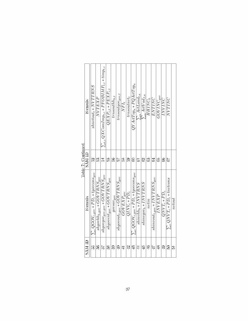
Table7:Continued

SAM

IDForm

ula

SAM

IDForm

ula

35

∑ cQGOVc,gov∗PD

c∗tgovcons g

ov

52

shnvtout t∗NVTTRNS

36

shgovhhh,gov∗GOVTRNSgov

53

NVTEXP

37

shgovgov

gov,gov∗GOVTRNSgov

54

∑ t,cQXCom

Impt,c∗PFOBIMPt,c∗timpt,c

38

shgovent g

ov∗GOVTRNSgov

55

QEXPc,t∗PEXPc,t

39

govsav g

ov

56

trnsouthhh,t

40

shgovout t,gov∗GOVTRNSgov

57

trnsoutgov

gov,t

41

GOVEXPgov

58

NFI t

42

QINVc∗PD

c59

trnsoutnvt t

43

∑ cQGOVc,gov∗PD

c∗tgovcons g

ov

60

QYActTop

a∗PQActTop

a

44

shinvhhh∗INVTRNS

61

∑ aActLandl,a

45

shinvgov

h∗INVTRNS

62

∑ aActVadf,a

46

nvtin

63

HHINC

h

47

shinvout t,gov∗INVTRNSgov

64

ENTINC

48

INVEXP

65

GOVINC

gov

49

QNVTc∗PD

c66

INVINC

50

∑ cQNVTc∗PD

c∗tnvtcons

67

NVTINC

51

nvtout

37

4 US Grain Sorghum Trade Flows

A policy research report presents the final results of a research project undertaken by AFPC faculty. At least a portion of the contents of this report may have been published previously as an AFPC issue paper or working paper. Since issue and working papers are preliminary reports, the final results contained in a research paper may differ - but, hopefully, in only marginal terms. Research reports are viewed by faculty of AFPC and the Department of Agricultural Economics, Texas A&M University. AFPC welcomes comments and discussions of these results and their implications. Address such comments to the author(s) at:

Agricultural and Food Policy Center Department of Agricultural Economics Texas A&M University College Station, Texas 77843-2124

or call (979) 845-5913.

Copies of this publication have been deposited with the Texas State Library in compliance with the State Depository Law.

Mention of a trademark or a proprietary product does not constitute a guarantee or a warranty of the product by Texas AgriLife Research or Texas AgriLife Extension Service and does not imply its approval to the exclusion of other products that also may be suitable.

All programs and information of Texas AgriLife Research or Texas AgriLife Extension Service are available to everyone without regard to race, color, religion, sex, age, handicap, or national origin.