A standard computable general equilibrium (CGE) model · PDF filea standard computable general...
79
Hans Lofgren Rebecca Lee Harris Sherman Robinson With assistance from Marcelle Thomas Moataz El-Said A Standard Computable General Equilibrium (CGE) INTERNATIONAL FOOD POLICY RESEARCH INSTITUTE sustainable options for ending hunger and poverty MICROCOMPUTERS IN POLICY RESEARCH 5
Transcript of A standard computable general equilibrium (CGE) model · PDF filea standard computable general...

Hans Lofgren
Rebecca Lee Harris
Sherman RobinsonWith assistance from
Marcelle Thomas
Moataz El-Said
A Standard ComputableGeneral Equilibrium (CGE)Model in GAMS
INTERNATIONAL FOOD POLICY RESEARCH INSTITUTE
sustainable options for ending hunger and poverty
MICROCOMPUTERS IN POLICY RESEARCH 5

The International Food Policy Research Institute (IFPRI)IFPRI was established in 1975 to identify and analyze national and international strategies andpolicies for meeting the food needs of the developing world on a sustainable basis, with partic-ular emphasis on low-income countries and poor people; to make the results of its researchavailable to all those in a position to use them; and to help strengthen institutions conductingresearch and applying research results in developing countries.
Future Harvest™ and the Consultative Group on InternationalAgricultural Research (CGIAR)IFPRI is one of 16 international food and environmental research organizations known as theFuture Harvest Centers. The Centers are principally funded by governments, private founda-tions, and regional and international organizations, most of which are members of the CGIAR.
About this SeriesMicrocomputers in Policy Research represents IFPRI’s ongoing collective experience in adaptingmicrocomputer technology for use in food policy analysis in developing countries. Designed toprovide hands-on methods and clear instruction through the extensive use of examples, the pri-mary purpose of the volumes in this series is to share IFPRI’s experience with potential develop-ing country users, although other users may find them helpful as well.
About GAMSThe General Algebraic Modeling System (GAMS) is a high-level modeling system for mathemati-cal programming problems. It consists of a language compiler and a stable of integrated high-performance solvers. GAMS is tailored for complex, large-scale modeling applications, andallows you to build large maintainable models that can be adapted quickly to new situations.GAMS allows the user to concentrate on the modeling problem by making the setup simple.The system takes care of the time-consuming details of the specific machine and system soft-ware implementation. For more information, visit www.gams.com.
Copyright © 2002 International Food Policy Research Institute. All rights reserved. Sections of this report may be reproduced with-out the express permission of but with acknowledgment to the International Food Policy Research Institute.
ISBN 0-896-29720-9
A STANDARD COMPUTABLE GENERAL EQUILIBRIUM (CGE)MODEL IN GAMS
HANS LOFGRENREBECCA LEE HARRISSHERMAN ROBINSON
with assistance fromMARCELLE THOMAS andMOATAZ EL-SAID
MICROCOMPUTERS IN POLICY RESEARCH 5INTERNATIONAL FOOD POLICY RESEARCH INSTITUTE
Copyright © 2002 International Food Policy Research Institute
All rights reserved. Sections of this book may be reproduced without the expresspermission of, but with acknowledgment to, the International Food Policy Research Institute.
International Food Policy Research Institute2033 K Street, N.W., Washington, D.C., 20006-1002, U.S.A.Telephone +1-202-862-5600; Fax +1-202-467-4439; www.ifpri.org
Library of Congress Cataloging-in-Publication DataLofgren, Hans.
A standard computable general equilibrium (CGE) model in GAMS / HansLofgren, Rebecca Lee Harris, Sherman Robinson ; with assistance from MarcelleThomas and Moataz El-Said.
p. cm.Includes bibliographical references and index.ISBN 0-89629-720-9 (alk. paper)
1. AgricultureEconomic aspectsMathematical models. 2. Food supplyMathematical models. 3. Equilibrium (Economics)Mathematicalmodels. I. Harris, Rebecca Lee, 1969- II. Robinson, Sherman. III.
Title.HD1415 .L64 2002338.1'01'51dc21 2002152627
iii
CONTENTS
Tables . . . . . . . . . . . . . . . . . . . . . . . . . . . . . . . . . . . . . . . . . . . . . . . . . . . . .iv
Figures . . . . . . . . . . . . . . . . . . . . . . . . . . . . . . . . . . . . . . . . . . . . . . . . . . . . .v
Preface . . . . . . . . . . . . . . . . . . . . . . . . . . . . . . . . . . . . . . . . . . . . . . . . . . . .vi
1. Introduction . . . . . . . . . . . . . . . . . . . . . . . . . . . . . . . . . . . . . . . . . . . . .1
2. The Social Accounting Matrix . . . . . . . . . . . . . . . . . . . . . . . . . . . . . . .3
3. Overview of the Standard CGE Model . . . . . . . . . . . . . . . . . . . . . . . .8
Institutions . . . . . . . . . . . . . . . . . . . . . . . . . . . . . . . . . . . . . . . . . . . . .10
Commodity Markets . . . . . . . . . . . . . . . . . . . . . . . . . . . . . . . . . . . . . .11
Macroeconomic Balances . . . . . . . . . . . . . . . . . . . . . . . . . . . . . . . . . .14
4. Mathematical Model Statement . . . . . . . . . . . . . . . . . . . . . . . . . . . .18
Price Block . . . . . . . . . . . . . . . . . . . . . . . . . . . . . . . . . . . . . . . . . . . . .18
Production and Trade Block . . . . . . . . . . . . . . . . . . . . . . . . . . . . . . .23
Institution Block . . . . . . . . . . . . . . . . . . . . . . . . . . . . . . . . . . . . . . . . .31
System Constraint Block . . . . . . . . . . . . . . . . . . . . . . . . . . . . . . . . . .35
5. The Standard Model in GAMS . . . . . . . . . . . . . . . . . . . . . . . . . . . . .42
Appendix A . . . . . . . . . . . . . . . . . . . . . . . . . . . . . . . . . . . . . . . . . . . . . . . .46
Appendix B . . . . . . . . . . . . . . . . . . . . . . . . . . . . . . . . . . . . . . . . . . . . . . . .60
References . . . . . . . . . . . . . . . . . . . . . . . . . . . . . . . . . . . . . . . . . . . . . . . . .68
TABLES
1. The Basic SAM structure used in the CGE model . . . . . . . . . . . . . . .5
2. Standard SAM for Zimbabwe, 1991 . . . . . . . . . . . . . . . . . . . . . . . . . . .6
3. Alternative closure rules for macrosystem constraints . . . . . . . . . . .13
4. Notational principles . . . . . . . . . . . . . . . . . . . . . . . . . . . . . . . . . . . . . .18
5. File structure in GAMS standard CGE modeling system . . . . . . . . .43
iv
FIGURES
1. Production technology . . . . . . . . . . . . . . . . . . . . . . . . . . . . . . . . . . . . . .9
2. Flows of marketed commodities . . . . . . . . . . . . . . . . . . . . . . . . . . . . .12
3. The structure of GAMS model and data files . . . . . . . . . . . . . . . . . .44
v
PREFACE
Over the past decade, the increasing power and reliability of microcom-puters and the development of sophisticated software designed specificallyfor use with them has led to significant changes in the way quantitativefood policy analysis is conducted. These changes cover most aspects of theanalysis, ranging from the collections and analysis of socioeconomic datato the conduct of model-based policy simulations. The venue of the com-putations has shifted from off-site mainframes dependent on highlytrained operators and significant capital investment in supporting equip-ment, to desktop and laptop computers dependent only on the occasionalavailability of electricity. This means that it is now feasible to quicklytransfer new techniques between IFPRI and its collaborators in develop-ing countries, that the costs of policy analysis have been substantially re-duced, and that a new level of complexity and accuracy in policy analysisis now possible.
As with any new technology, however, substantial costs in time andmoney are involved in learning the most efficient ways of using this newtechnology and then transmitting these lessons to others. This series, Mi-crocomputers in Policy Research, represents IFPRI's ongoing collective ex-perience in adapting microcomputer technology for use in food policyanalysis in developing countries. Publication decisions are made on thebasis of a review by an external referee. The manuals in the series are pri-marily for the purpose of sharing these lessons with potential users in de-veloping countries, although persons and institutions in developed coun-tries may also find them useful. The series is designed to provide hands-on methods for quantities food policy analysis. In our opinion, examplesprovide the best and clearest form of instruction; therefore, examplesin-cluding actual software codes wherever relevantare used extensivelythroughout this series.
Computable general equilibrium (CGE) models are used widely in pol-icy analysis, especially in developed-country academic settings. The pur-pose of the fifth volume in the series, A Standard Computable GeneralEquilibrium (CGE) Model in GAMS, by Hans Lofgren, Rebecca Lee Har-ris, and Sherman Robinson, with assistance from Marcelle Thomas andMoataz El-Said, is to contribute to and facilitate the use of this class ofmodels in developing countries. The volume includes a detailed presenta-tion of a static "standard" CGE model and its required database. Themodel is written for application at the country level; however, only mini-mal changes are needed before it can be applied to a region within a coun-try (such as a village) or to a farm household involved in production andconsumption activities. The model incorporates features developed overrecent years through IFPRI's research projects. These featuresof partic-ular importance in developing countriesinclude household consumptionof nonmarketed ("home") commodities, explicit treatment of transactioncosts for commodities that enter the market sphere, and a separation be-tween production activities and commodities that permits any activity toproduce multiple commodities and any commodity to be produced by mul-tiple activities. The manual discusses the implementation of the model inGAMS (the General Algebraic Modeling System) and is accompanied by aCD-ROM that includes the GAMS files for the model, sample databases,simulations, solution reports, and a social accounting matrix (SAM)
vi
aggregation program. Although the volume provides a standardizedframework for analysis, the analyst is not forced to make "one-size-fits-all"assumptions. The GAMS code is written to give the analyst considerableflexibility in model specification.
Howarth Bouis and Hans Lofgren, Series Editors
vii
INTRODUCTION
Over the past 25 years, computable general equilibrium (CGE) modelshave become a standard tool of empirical economic analysis. In recentyears, improvements in model specification, data availability, and com-puter technology have improved the payoffs and reduced the costs of pol-icy analysis based on CGE models, paving the way for their widespreaduse by policy analysts throughout the world. The purpose of this manualis to contribute to and facilitate the use of CGE models, making them ac-cessible to a wider group of economists. The manual includes a detailedpresentation of a static, standard CGE model implemented in a com-puter modeling language called GAMS (General Algebraic Modeling Sys-tem). It also provides a sample database in an accompanying CD-ROM.1
Although most CGE models have been developed for countries, thebasic framework applies, and has been applied, in settings ranging fromthe world (divided into multiple regions) to disaggregated regions withina country, such as villages, and even to households. In most applications,the markets and prices in the model represent actual markets with moneyused as a medium of exchange. However, especially in household models,they may be viewed as implicit markets where the solution wages andprices represent shadow prices or exchange values. Our standardCGE model is written for application at the country level and has been im-plemented with a number of country data sets, but only minimal changesare needed to apply the model to a region within a country or to a pro-ducer-consumer household.
The standard model includes a number of features designed to reflectthe characteristics of developing countries. The specification follows theneoclassical-structuralist modeling tradition presented in Dervis et al.(1982). It incorporates additional features developed in recent years in re-search projects conducted at IFPRI. These features, of particular impor-tance in developing countries, include household consumption of nonmar-keted (or home) commodities, explicit treatment of transaction costs forcommodities that enter the market sphere, and a separation between pro-duction activities and commodities that permits any activity to produce
The authors would like to thank Ed Taylor for a constructive review, and Renger vanNieuwkoop and Jennifer Chung-I Li for useful comments.1We assume that the reader has a basic familiarity with CGE modeling using GAMS.Brooke et al. (1998) is the basic reference on the GAMS software; it also includes aself-contained tutorial. The basics of GAMS-based CGE modeling are summarized inRobinson et al. (1999). Lofgren (2000a, 2000b) presents a set of hands-on exercisesin CGE modeling with GAMS. Extensive treatments of CGE methods are found inDervis et al. (1982), Robinson (1989), Shoven and Whalley (1992), Dixon et al.(1992), and Ginsburgh and Keyzer (1997). References to and examples of CGE-basedanalyses of food policy in developing countries are found in the Trade and Macro-economics Division section of the IFPRI website (www.ifpri.org).
1.
1
multiple commodities and any commodity to be produced by multiple ac-tivities.
The CD-ROM provided includes the GAMS files for the CGE model,sample databases, simulations, solution reports, and a social accountingmatrix (SAM) aggregation program. In the GAMS code, the model is ex-plicitly linked to a file for country data, including a standard SAM thatfollows the format required for the standard CGE model and a set of elas-ticities. Optionally, the user may provide quantity data for primary factors(for example, labor types) that appear in the SAM. In the model code, thisdata set is used to define model parameter values in a manner that assuresthat the base solution to the model exactly reproduces the values in theSAM. In other words, the model is calibrated to the SAM. It is, more-over, straightforward for users to develop new data sets for other applica-tions.
The CGE model and the accompanying GAMS code are written to giveanalysts considerable flexibility. He or she can choose between alternativetreatments for macroeconomic balances and for factor markets. It is alsopossible to exclude various features that appear in the standard model,such as home consumption and transaction costs. The country database towhich the model should be applied can incorporate a wide range of policytools as well as any desired degree of disaggregation of production activi-ties, commodities, households, and enterprises. Flexibility in terms ofmodel structure and the fact that model parameters are derived from anempirical database (which may be very detailed) permit the analyst to cap-ture country-specific aspects of economic structure and functioning.Hence, although the manual provides a standardized framework foranalysis, the analyst is not forced to make one-size-fits-all assumptions.
We consider this CGE model and the accompanying computer code aswork in progress and encourage readers and users to send us their com-ments. A number of extensions are possible. For example, users may be in-terested in adding alternative treatments of production technology or amore detailed treatment of policy tools. However, when new features areadded, there is a tradeoff between additional versatility and additionalcomplexity. Unless the new features are of general interest, they shouldpreferably be added in the context of specific applications that use the cur-rent, relatively simple model as their starting point. As noted earlier, themodel can be easily adapted for application to regions within a country orto a household that is involved in production and consumption. More fun-damental changes would be needed to make it dynamic or to turn it into aworld model.2
The remainder of this manual is organized as follows: Chapter 2 de-scribes the standard SAM. Chapter 3 provides an overview of the featuresof the CGE model, followed by an equation-by-equation description inChapter 4. Chapter 5 describes the structure of the GAMS files for thestandard CGE model and its database and discusses how they may be usedfor policy analysis. The appendixes include the mathematical model state-ment in summary form and core sections of the GAMS code for the model.
2To apply the model to a region or a household, the only changes needed involve theaddition of new rules for closing the accounts for the government and the rest of theworld (now representing the economy outside the region or the household). Thedatabase (including the SAM) should then represent a region or a farm household.
2
3
THE SOCIAL ACCOUNTING MATRIX
A social accounting matrix (SAM) is a comprehensive, economywide dataframework, typically representing the economy of a nation.3 More techni-cally, a SAM is a square matrix in which each account is represented by arow and a column. Each cell shows the payment from the account of itscolumn to the account of its row. Thus, the incomes of an account appearalong its row and its expenditures along its column. The underlying prin-ciple of double-entry accounting requires that, for each account in theSAM, total revenue (row total) equals total expenditure (column total).4
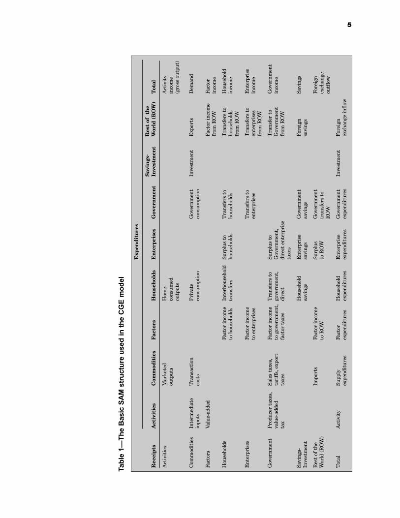
Table 1 shows an aggregated SAM with verbal explanations in the cellsinstead of numbers. With one exception, it has all of the features requiredfor implementation with the standard CGE model. The exception is thatin the standard SAM, taxes have to be paid to tax accounts, disaggregatedby tax type, each of which forwards its revenues to the core governmentaccount. The tax types are divided into direct taxes (on domestic non-government institutions and factors), commodity sales taxes, importtaxes, export taxes, activity taxes, and value-added taxes. Also note that,in the standard SAM, payments are not permitted in the blank cells ofTable 1. Any original SAM that includes such payments should be re-structured before being implemented with the standard CGE model.5
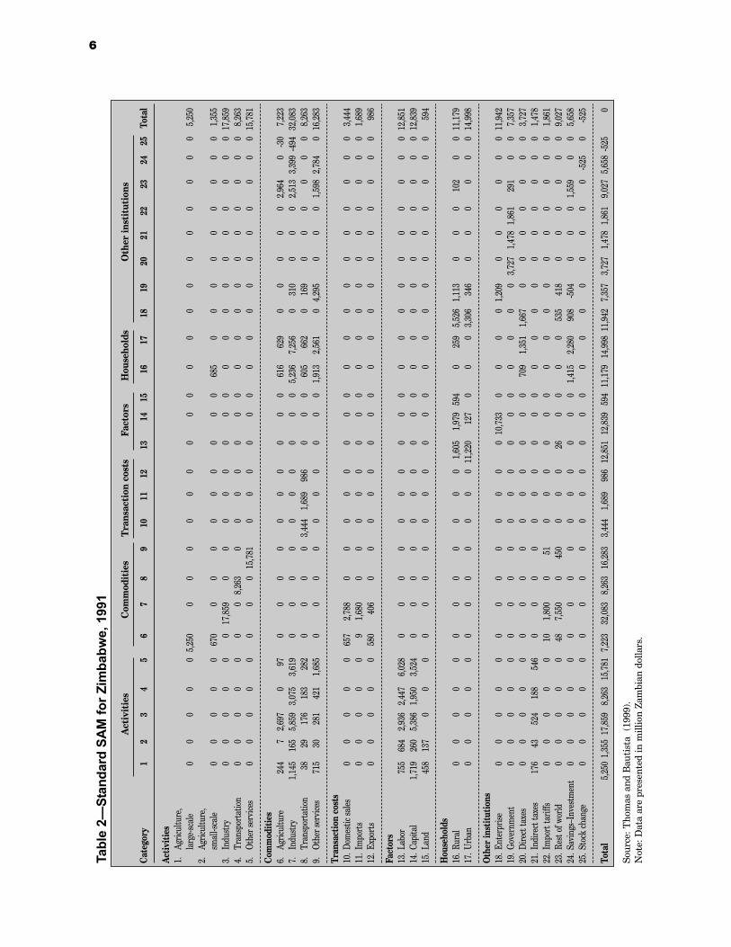
Table 2 shows a real-world standard SAM for Zimbabwe in which thetax accounts are treated in the required manner.6 In addition, it has mul-tiple accounts for activities, commodities, factors, and domestic non-
3For general discussions of SAMs, see Pyatt and Round (1985) and Reinert andRoland-Holst (1997); for perspectives on SAM-based modeling, see Pyatt (1988) andRobinson and Roland-Holst (1988).4The GAMS program checks that the SAM that is entered is balanced (meaning therow and column totals are equal for each account). If the absolute value of the sumof account imbalances exceeds a cutoff point, an optimization program is used to es-timate a balanced SAM. The program, which minimizes the entropy distance of thecells of the estimated SAM from those of the initial SAM subject to the constraintthat row and column totals are equal, is primarily intended to remove rounding er-rors. For SAM estimation in GAMS in a setting with substantial imbalances in rawdata (not only rounding errors), see Robinson and El-Said (2000) and Robinson, Cat-taneo, and El-Said (2001).5One common case would be payments from the government to factors (for the laborservices provided by government employees). To restructure the SAM to work withthe standard model, the preferred approach is to reallocate such payments to acommodity for government services that pays a government service activity which,in turn, pays the labor account. 6For other examples of SAMs that have the required structure, see the data setspage on IFPRIs website (www.ifpri.org).
2.
government institutions. In each category, the GAMS code can handle anydesired disaggregation, including having just a single account. In any real-world application, the preferred disaggregation of the SAM and the CGEmodel depends on data availability and the purposes of the analysis. It istypically preferable to include relatively detailed treatment in areas of in-terest while keeping the database relatively aggregated in other areas.7
With regard to the structure of the standard SAM, a number of fea-tures are noteworthy. First, the standard SAM distinguishes between ac-counts for activities (the entities that carry out production) and com-modities. The receipts are valued at producer prices in the activity ac-counts and at market prices (including indirect commodity taxes andtransaction costs) in the commodity accounts. The commodities are activ-ity outputs, either exported or sold domestically, and imports. This sepa-ration of activities from commodities is preferred because it permits ac-tivities to produce multiple commodities (for example, a dairy activity mayproduce the commodities cheese and milk) while any commodity may beproduced by multiple activities (for example, activities for small-scale andlarge-scale maize production may both produce the same maize commod-ity). In the commodity columns, payments are made to domestic activities,the rest of the world, and various tax accounts (for domestic and importtaxes). This treatment provides the data needed to model imports as per-fect or imperfect substitutes vis-à-vis domestic production.8
Second, the matrix explicitly associates trade flows with transactions(trade and transportation) costs, also referred to as marketing margins.For each commodity, the SAM accounts for the costs associated with do-mestic, import, and export marketing. For domestic marketing of domes-tic output, the marketing margin represents the cost of moving the com-modity from the producer to the domestic demander. For imports, it rep-resents the cost of moving the commodity from the border (adding to thec.i.f. price) to the domestic demander, while for exports, it shows the costof moving the commodity from the producer to the border (reducing theprice received by producers relative to the f.o.b. price). The ZimbabweSAM in Table 2 shows how these transaction costs appear in commodityand activity accounts in the standard SAM: A services activity, in Table 2called transportation (account 4), produces a commodity (account 8) that,like other commodities, may be purchased for intermediate use by activi-ties and for final use by institutions. However, the transportation commodity also receives payments from three special accounts, represent-ing the transaction costs associated with domestic sales, imports, and exports (accounts 10-12).9 These special accounts are paid by the accounts
7The CD-ROM that accompanies this manual includes a program for aggregating anexisting SAM.8In addition, our model code makes it possible to treat selected imports as separate,noncomparable commodities (not produced domestically). In the commodity rows,such import commodities receive payments from one or more domestic users. In thecolumns, these payments would be passed on to the accounts for the rest of theworld, import marketing margins, and relevant taxes. The columns for this categoryof imports do not have any payments to domestic activities.
4
Tabl
e 1
The
Basi
c SA
M s
truct
ure
used
in th
e CG
E m
odel
Exp
end
itu
res
Sav
ings
- R
est
of
the
Rec
eip
tsA
ctiv
itie
sC
omm
odit
ies
Fac
tors
Hou
seh
old
sE
nte
rpri
ses
Gov
ern
men
tIn
vest
men
tW
orld
(R
OW
)T
otal
Act
ivit
ies
Mar
kete
dH
ome-
Act
ivit
y ou
tput
sco
nsum
ed
inco
me
outp
uts
(gro
ss o
utpu
t)
Com
mod
itie
sIn
term
edia
te
Tra
nsac
tion
P
riva
te
Gov
ernm
ent
Inve
stm
ent
Exp
orts
Dem
and
inpu
tsco
sts
cons
umpt
ion
cons
umpt
ion
Fact
ors
Valu
e-ad
ded
Fact
or in
com
e Fa
ctor
fr
om R
OW
inco
me
Hou
seho
lds
Fact
or in
com
e In
terh
ouse
hold
Su
rplu
s to
T
rans
fers
to
Tra
nsfe
rs t
o H
ouse
hold
to h
ouse
hold
str
ansf
ers
hous
ehol
dsho
useh
olds
hous
ehol
ds
inco
me
from
RO
W
Ent
erpr
ises
Fact
or in
com
eT
rans
fers
to
Tra
nsfe
rs t
o E
nter
pris
e to
ent
erpr
ises
ente
rpri
ses
ente
rpri
ses
inco
me
from
RO
W
Gov
ernm
ent
Pro
duce
r ta
xes,
Sale
s ta
xes,
Fa
ctor
inco
me
Tra
nsfe
rs t
oSu
rplu
s to
Tra
nsfe
r to
Gov
ernm
ent
valu
e-ad
ded
tari
ffs,
exp
ort
to g
over
nmen
t,go
vern
men
t,G
over
nmen
t,G
over
nmen
t in
com
eta
xta
xes
fact
or t
axes
dire
ctdi
rect
ent
erpr
ise
from
RO
Wta
xes
Savi
ngs-
H
ouse
hold
Ent
erpr
ise
Gov
ernm
ent
Fore
ign
Savi
ngs
Inve
stm
ent
savi
ngs
savi
ngs
savi
ngs
savi
ngs
Res
t of
the
Im
port
sFa
ctor
inco
me
Surp
lus
Gov
ernm
ent
Fore
ign
Wor
ld (
RO
W)
to R
OW
to R
OW
tran
sfer
s to
ex
chan
ge
RO
Wou
tflo
w
Tot
alA
ctiv
ity
Supp
lyFa
ctor
H
ouse
hold
E
nter
pris
e G
over
nmen
tIn
vest
men
tFo
reig
n ex
pend
itur
esex
pend
itur
esex
pend
itur
esex
pend
itur
esex
pend
itur
esex
chan
ge in
flow
5
Tabl
e 2
Stan
dard
SAM
for Z
imba
bwe,
199
1A
ctiv
itie
sC
omm
odit
ies
Tra
nsac
tion
cos
tsFa
ctor
sH
ouse
hold
sO
ther
inst
itut
ions
Cat
egor
y1
23
45
67
89
1011
1213
1415
1617
1819
2021
2223
2425
Tota
l
Acti
viti
es1.
Agric
ultu
re,
larg
e-sc
ale
00
00
05,
250
00
00
00
00
00
00
00
00
00
05,
250
2.Ag
ricul
ture
, sm
all-s
cale
00
00
067
00
00
00
00
00
685
00
00
00
00
01,
355
3.In
dust
ry0
00
00
017
,859
00
00
00
00
00
00
00
00
00
17,8
594.
Tran
spor
tatio
n0
00
00
00
8,26
30
00
00
00
00
00
00
00
00
8,26
35.
Oth
er se
rvice
s0
00
00
00
015
,781
00
00
00
00
00
00
00
00
15,7
81
Com
mod
itie
s6.
Agric
ultu
re24
47
2,69
70
970
00
00
00
00
061
662
90
00
00
2,96
40
-30
7,22
37.
Indu
stry
1,14
516
55,
859
3,07
53,
619
00
00
00
00
00
5,23
67,
256
031
00
00
2,51
33,
399
-494
32,0
838.
Tr
ansp
orta
tion
3829
176
183
282
00
00
3,44
41,
689
986
00
060
566
20
169
00
00
00
8,26
39.
O
ther
serv
ices
715
3028
142
11,
685
00
00
00
00
00
1,91
32,
561
04,
295
00
01,
598
2,78
40
16,2
83
Tran
sact
ion
cost
s10
. Dom
estic
sale
s0
00
00
657
2,78
80
00
00
00
00
00
00
00
00
03,
444
11. I
mpo
rts
00
00
09
1,68
00
00
00
00
00
00
00
00
00
01,
689
12. E
xpor
ts0
00
00
580
406
00
00
00
00
00
00
00
00
00
986
Fact
ors
13. L
abor
755
684
2,93
62,
447
6,02
80
00
00
00
00
00
00
00
00
00
012
,851
14. C
apita
l1,
719
260
5,38
61,
950
3,52
40
00
00
00
00
00
00
00
00
00
012
,839
15. L
and
458
137
00
00
00
00
00
00
00
00
00
00
00
059
4
Hou
seho
lds
16. R
ural
00
00
00
00
00
00
1,60
51,
979
594
025
95,
526
1,11
30
00
102
00
11,1
7917
. Urb
an0
00
00
00
00
00
011
,220
127
00
03,
306
346
00
00
00
14,9
98
Oth
er in
stit
utio
ns18
. Ent
erpr
ise0
00
00
00
00
00
00
10,7
330
00
01,
209
00
00
00
11,9
4219
. Gov
ernm
ent
00
00
00
00
00
00
00
00
00
03,
727
1,47
81,
861
291
00
7,35
720
. Dire
ct ta
xes
00
00
00
00
00
00
00
070
91,
351
1,66
70
00
00
00
3,72
721
. Ind
irect
taxe
s17
643
524
188
546
00
00
00
00
00
00
00
00
00
00
1,47
822
. Im
port
tarif
fs0
00
00
101,
800
051
00
00
00
00
00
00
00
00
1,86
123
. Res
t of w
orld
00
00
048
7,55
00
450
00
026
00
00
535
418
00
00
00
9,02
724
. Sav
ings
Inv
estm
ent
00
00
00
00
00
00
00
01,
415
2,28
090
8-5
040
00
1,55
90
05,
658
25. S
tock
chan
ge0
00
00
00
00
00
00
00
00
00
00
00
-525
0-5
25
Tota
l5,
250
1,35
517
,859
8,26
315
,781
7,22
332
,083
8,26
316
,283
3,44
41,
689
986
12,8
5112
,839
594
11,1
7914
,998
11,9
427,
357
3,72
71,
478
1,86
19,
027
5,65
8-5
250
Sour
ce: T
hom
as a
nd B
auti
sta
(19
99).
Not
e: D
ata
are
pres
ente
d in
mill
ion
Zam
bian
dol
lars
.
6
for marketed agricultural and industrial commodities (accounts 6 and 7).Thus the total value of each commodity includes these transaction costs.The standard CGE model will also work with SAMs without this treat-ment of (and these accounts for) transaction costs.
Third, as noted, the government is disaggregated into a core govern-ment account and different tax accounts, one for each tax type. This dis-aggregation is often necessary because the economic interpretation ofsome payments may otherwise be ambiguous. In any given application,the SAM may exclude any (or all) of the individual tax accounts. In theSAM, payments between the government and other domestic institutionsare reserved for transfers.
Fourth, the domestic nongovernment institutions in the SAM consistof households and enterprises. The enterprises earn factor incomes (re-flecting their ownership of capital and/or land). They may also receivetransfers from other institutions. Their incomes are used for direct taxes,savings, and transfers to other institutions. As opposed to households, en-terprises do not consume. Assuming that the relevant data are available,it is preferable to have one or more accounts for enterprises when thesehave tax obligations and a savings behavior that are independent of thehousehold sector. The enterprise sector should be disaggregated in a man-ner that captures differences across enterprises in terms of tax rates, sav-ings rates, and the shares of retained earnings that are received by differ-ent household types. For example, in some settings it may be appropriateto disaggregate enterprises into the categories nonagricultural (meaningearnings from nonagricultural capital), small-scale agricultural (earningsfrom land and capital controlled by small farmers), and large-scale agri-cultural (earnings from land and capital of large farmers). Technically, thestandard CGE model requires that the SAM have at least one householdaccount; enterprise accounts are not necessary.
Finally, the SAM distinguishes between home consumption, which isactivity-based, and households marketed consumption, which is commod-ity-based. Home consumption, which in the SAM appears as householdpayments to activities, is valued at producer pricesthat is, without mar-keting margins and the sales taxes that may be imposed on marketed com-modities.10 Household consumption of marketed commodities appears aspayments from household accounts to commodity accounts, the values ofwhich include marketing margins and commodity taxes. The standardCGE model also accepts a SAM without (explicit) home consumption.
7
9The distinction between intermediate use of transportation services and their usein output marketing (giving rise to transaction costs) is that intermediate input useis part of the production process whereas use in marketing is incurred only if theoutput is actually marketed (as opposed to being home-consumed). Input-output ta-bles typically include information on marketing margins but in a less (or differently)disaggregated format than that proposed for the standard model SAM. Hence, addi-tional data and analysis may be needed if the model user wishes to construct a SAMwith the proposed treatment of marketing margins.10In the model, home consumption demand is for the commodity output(s) of the ac-tivities that, in the SAM, receive payments from households (compare with footnote7 and equations 18 and 34 in Chapter 4).
OVERVIEW OF THE STANDARDCGE MODEL
The standard CGE model explains all of the payments recorded in theSAM. The model therefore follows the SAM disaggregation of factors, ac-tivities, commodities, and institutions. It is written as a set of simultane-ous equations, many of which are nonlinear. There is no objective func-tion. The equations define the behavior of the different actors. In part,this behavior follows simple rules captured by fixed coefficients (for ex-ample, ad valorem tax rates). For production and consumption decisions,behavior is captured by nonlinear, first-order optimality conditionsthatis, production and consumption decisions are driven by the maximizationof profits and utility, respectively. The equations also include a set of con-straints that have to be satisfied by the system as a whole but are not nec-essarily considered by any individual actor. These constraints cover mar-kets (for factors and commodities) and macroeconomic aggregates (bal-ances for SavingsInvestment, the government, and the current accountof the rest of the world).
This chapter summarizes the basic characteristics of the model. Un-like the more detailed presentation in Chapter 4, it uses no mathematicalnotation.
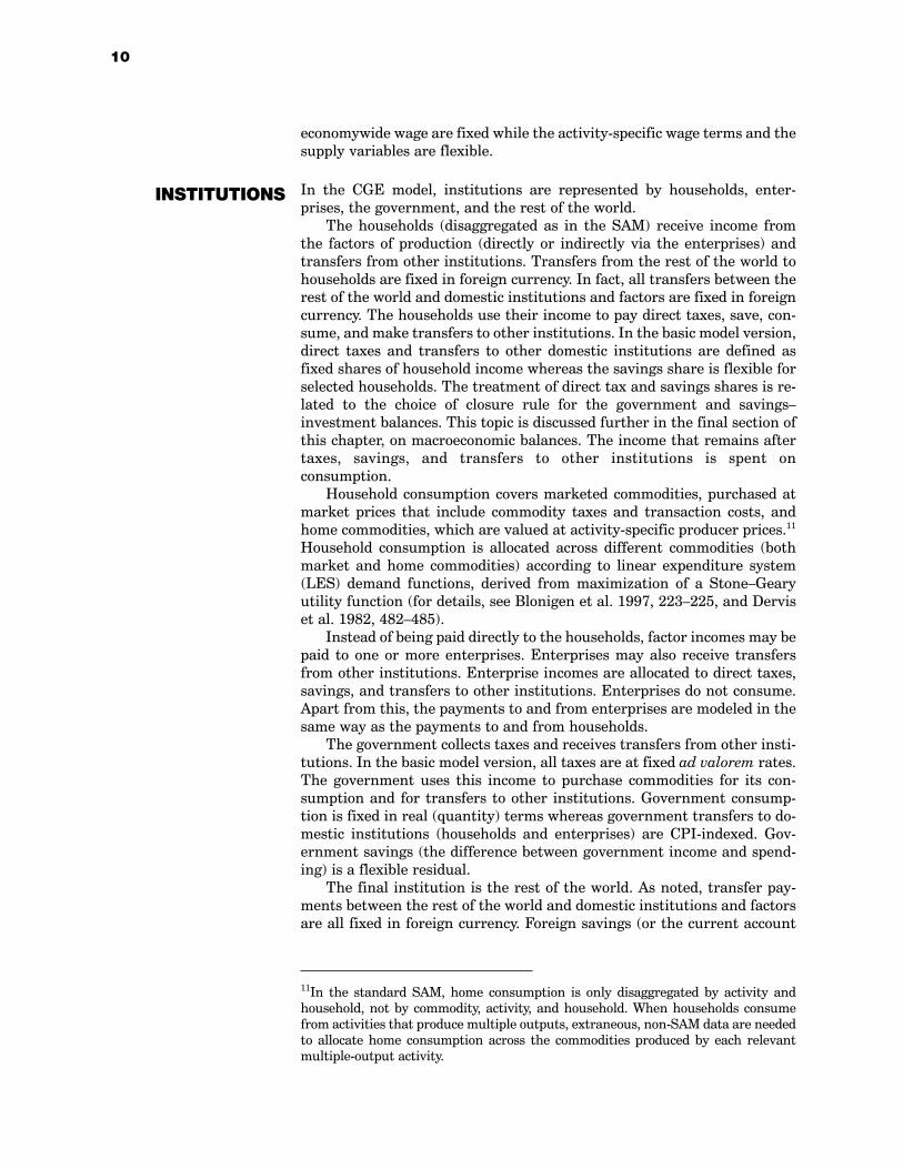
Each producer (represented by an activity) is assumed to maximize prof-its, defined as the difference between revenue earned and the cost of fac-tors and intermediate inputs. Profits are maximized subject to a produc-tion technology, the structure of which is shown in Figure 1. At the toplevel, the technology is specified by a constant elasticity of substitution(CES) function or, alternatively, a Leontief function of the quantities ofvalue-added and aggregate intermediate input. The Leontief alternative isthe default. The CES alternative may be preferable for particular sectorsif empirical evidence suggests that available techniques permit the aggre-gate mix between value-added and intermediate inputs to vary. Value-added is itself a CES function of primary factors whereas the aggregate in-termediate input is a Leontief function of disaggregated intermediate inputs.
Each activity produces one or more commodities according to fixedyield coefficients. As noted, a commodity may be produced by more thanone activity. The revenue of the activity is defined by the level of the activity, yields, and commodity prices at the producer level.
As part of its profit-maximizing decision, each activity uses a set of fac-tors up to the point where the marginal revenue product of each factor isequal to its wage (also called factor price or rent). Factor wages may differacross activities, not only when the market is segmented but also for mo-bile factors. In the latter case, the model incorporates discrepancies thatstem from exogenous causes (for example, wage differences across activi-ties resulting from considerations such as status, comfort, or health risks).
ACTIVITIES, PRODUCTION,AND FACTOR
MARKETS
3.
8
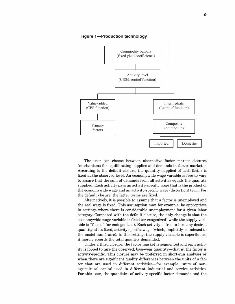
The user can choose between alternative factor market closures(mechanisms for equilibrating supplies and demands in factor markets).According to the default closure, the quantity supplied of each factor isfixed at the observed level. An economywide wage variable is free to varyto assure that the sum of demands from all activities equals the quantitysupplied. Each activity pays an activity-specific wage that is the product ofthe economywide wage and an activity-specific wage (distortion) term. Forthe default closure, the latter terms are fixed.
Alternatively, it is possible to assume that a factor is unemployed andthe real wage is fixed. This assumption may, for example, be appropriatein settings where there is considerable unemployment for a given laborcategory. Compared with the default closure, the only change is that theeconomywide wage variable is fixed (or exogenized) while the supply vari-able is flexed (or endogenized). Each activity is free to hire any desiredquantity at its fixed, activity-specific wage (which, implicitly, is indexed tothe model numéraire). In this setting, the supply variable is superfluous;it merely records the total quantity demanded.
Under a third closure, the factor market is segmented and each activ-ity is forced to hire the observed, base-year quantitythat is, the factor isactivity-specific. This closure may be preferred in short-run analyses orwhen there are significant quality differences between the units of a fac-tor that are used in different activitiesfor example, units of non-agricultural capital used in different industrial and service activities. For this case, the quantities of activity-specific factor demands and the
9
Intermediate
(Leontief function)
Activity level
(CES/Leontief function)
Composite
commodities
Value-added
(CES function)
Primary
factors
Commodity outputs
(fixed yield coefficients)
Imported Domestic
Figure 1—Production technology
economywide wage are fixed while the activity-specific wage terms and thesupply variables are flexible.
In the CGE model, institutions are represented by households, enter-prises, the government, and the rest of the world.
The households (disaggregated as in the SAM) receive income fromthe factors of production (directly or indirectly via the enterprises) andtransfers from other institutions. Transfers from the rest of the world tohouseholds are fixed in foreign currency. In fact, all transfers between therest of the world and domestic institutions and factors are fixed in foreigncurrency. The households use their income to pay direct taxes, save, con-sume, and make transfers to other institutions. In the basic model version,direct taxes and transfers to other domestic institutions are defined asfixed shares of household income whereas the savings share is flexible forselected households. The treatment of direct tax and savings shares is re-lated to the choice of closure rule for the government and savingsinvestment balances. This topic is discussed further in the final section ofthis chapter, on macroeconomic balances. The income that remains aftertaxes, savings, and transfers to other institutions is spent on consumption.
Household consumption covers marketed commodities, purchased atmarket prices that include commodity taxes and transaction costs, andhome commodities, which are valued at activity-specific producer prices.11
Household consumption is allocated across different commodities (bothmarket and home commodities) according to linear expenditure system(LES) demand functions, derived from maximization of a StoneGearyutility function (for details, see Blonigen et al. 1997, 223225, and Derviset al. 1982, 482485).
Instead of being paid directly to the households, factor incomes may bepaid to one or more enterprises. Enterprises may also receive transfersfrom other institutions. Enterprise incomes are allocated to direct taxes,savings, and transfers to other institutions. Enterprises do not consume.Apart from this, the payments to and from enterprises are modeled in thesame way as the payments to and from households.
The government collects taxes and receives transfers from other insti-tutions. In the basic model version, all taxes are at fixed ad valorem rates.The government uses this income to purchase commodities for its con-sumption and for transfers to other institutions. Government consump-tion is fixed in real (quantity) terms whereas government transfers to do-mestic institutions (households and enterprises) are CPI-indexed. Gov-ernment savings (the difference between government income and spend-ing) is a flexible residual.
The final institution is the rest of the world. As noted, transfer pay-ments between the rest of the world and domestic institutions and factorsare all fixed in foreign currency. Foreign savings (or the current account
10
11In the standard SAM, home consumption is only disaggregated by activity andhousehold, not by commodity, activity, and household. When households consumefrom activities that produce multiple outputs, extraneous, non-SAM data are neededto allocate home consumption across the commodities produced by each relevantmultiple-output activity.
INSTITUTIONS
deficit) is the difference between foreign currency spending and receipts.Commodity trade with the rest of the world is discussed in the next sec-tion. Thereafter, the final section of this chapter discusses the rules forclearing the macroeconomic balances (the macroclosures)that is, howequilibrium is achieved in the balances for the government, the rest of theworld, and the SavingsInvestment account (where institutional savingsare aggregated and allocated to domestic investment).
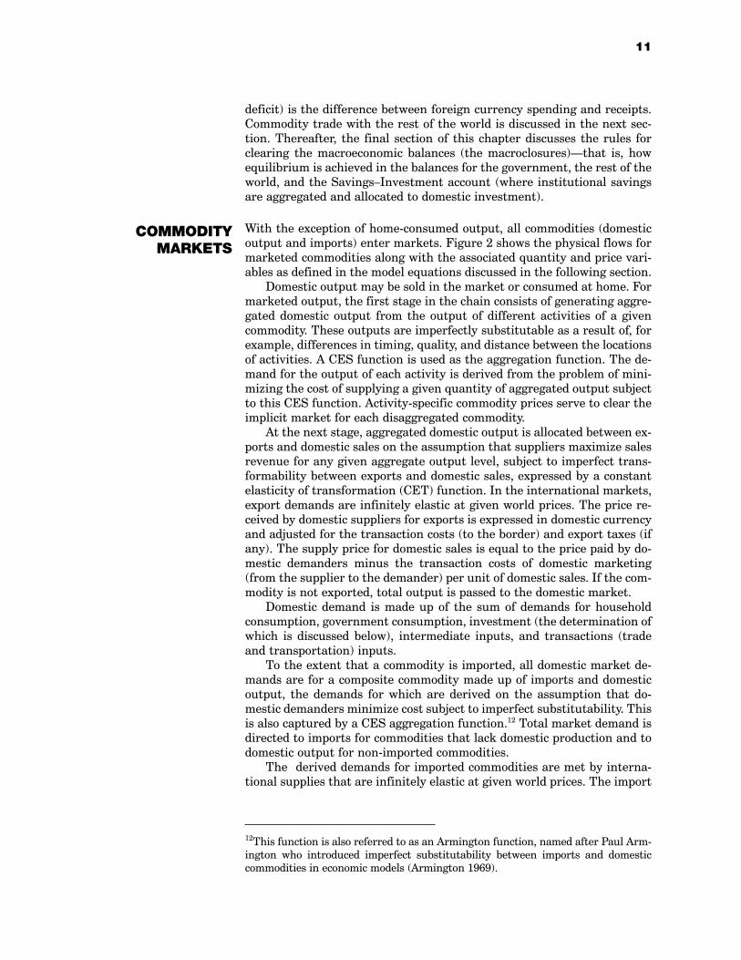
With the exception of home-consumed output, all commodities (domesticoutput and imports) enter markets. Figure 2 shows the physical flows formarketed commodities along with the associated quantity and price vari-ables as defined in the model equations discussed in the following section.
Domestic output may be sold in the market or consumed at home. Formarketed output, the first stage in the chain consists of generating aggre-gated domestic output from the output of different activities of a givencommodity. These outputs are imperfectly substitutable as a result of, forexample, differences in timing, quality, and distance between the locationsof activities. A CES function is used as the aggregation function. The de-mand for the output of each activity is derived from the problem of mini-mizing the cost of supplying a given quantity of aggregated output subjectto this CES function. Activity-specific commodity prices serve to clear theimplicit market for each disaggregated commodity.
At the next stage, aggregated domestic output is allocated between ex-ports and domestic sales on the assumption that suppliers maximize salesrevenue for any given aggregate output level, subject to imperfect trans-formability between exports and domestic sales, expressed by a constantelasticity of transformation (CET) function. In the international markets,export demands are infinitely elastic at given world prices. The price re-ceived by domestic suppliers for exports is expressed in domestic currencyand adjusted for the transaction costs (to the border) and export taxes (ifany). The supply price for domestic sales is equal to the price paid by do-mestic demanders minus the transaction costs of domestic marketing(from the supplier to the demander) per unit of domestic sales. If the com-modity is not exported, total output is passed to the domestic market.
Domestic demand is made up of the sum of demands for householdconsumption, government consumption, investment (the determination ofwhich is discussed below), intermediate inputs, and transactions (tradeand transportation) inputs.
To the extent that a commodity is imported, all domestic market de-mands are for a composite commodity made up of imports and domesticoutput, the demands for which are derived on the assumption that do-mestic demanders minimize cost subject to imperfect substitutability. Thisis also captured by a CES aggregation function.12 Total market demand isdirected to imports for commodities that lack domestic production and todomestic output for non-imported commodities.
The derived demands for imported commodities are met by interna-tional supplies that are infinitely elastic at given world prices. The import
11
12This function is also referred to as an Armington function, named after Paul Arm-ington who introduced imperfect substitutability between imports and domesticcommodities in economic models (Armington 1969).
COMMODITY MARKETS
12
CE
S
Co
mm
od
ity
ou
tpu
tfr
om
acti
vit
y1
(QX
AC
|
PX
AC
)
Co
mm
odit
y
ou
tpu
tfr
om
acti
vit
yn
(QX
AC
|
PX
AC
)
Aggre
gate
outp
ut
(QX
|P
X)
CE
T
Ag
gre
gate
imp
ort
s
(QM
|P
M)
Ag
gre
gate
ex
po
rts
(QE
|P
E)
CE
SC
om
posit
e
co
mm
odit
y
|P
Q)
Household
consum
pti
on
(QH
|P
Q)
+
Govern
ment
consum
pti
on
(QG
|P
Q)
+
Investm
ent
(QIN
V+
qdst
|
PQ
)
+
Inte
rmedia
teuse
(QIN
T|P
Q)
. . .
Do
mesti
c
sale
s
(QD
|P
DS-
PD
D)
Fig
ure
2—
Flo
ws o
f m
ark
ete
d c
om
mo
dit
ies
Note
:C
ES
iscon
sta
nt
ela
sti
cit
yof
su
bsti
tuti
on
;C
ET
iscon
sta
nt
ela
sti
cit
yof
tra
nsfo
rm
ati
on
.
prices paid by domestic demanders also include import tariffs (at fixed advalorem rates) and the cost of a fixed quantity of transactions services perimport unit, covering the cost of moving the commodity from the borderto the demander.13 Similarly, the derived demand for domestic output ismet by domestic suppliers. The prices paid by the demanders include thecost of transactions services, in this case reflecting that the commoditywas moved from the domestic supplier to the domestic demander. Theprices received by domestic suppliers are net of these transaction costs.Flexible prices equilibrate demands and supplies of domestically marketeddomestic output.
Compared with the alternative assumptions of perfect substitutabilityand transformability, the assumptions of imperfect transformability (be-tween exports and domestic sales of domestic output) and imperfect sub-stitutability (between imports and domestically sold domestic output)
13
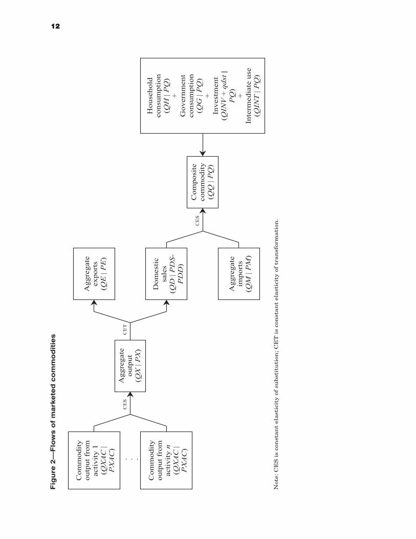
Table 3Alternative closure rules for macrosystem constraints
Constraint
Government Rest of the World SavingsInvestment
GOV-1: ROW-1: SI-1:Flexible government Fixed foreign savings; Fixed capital formation;savings; fixed direct flexible real exchange rate uniform MPS point change tax rates for selected institutions
GOV-2: ROW-2: SI-2:Fixed government savings; Flexible foreign savings; Fixed capital formation; uniform direct tax rate fixed real exchange rate scaled MPS for selectedpoint change for selected institutionsinstitutions
GOV-3: SI-3:Fixed government savings; Flexible capital formation;scaled direct tax rates for fixed MPS for all nonselected institutions government institutions
SI-4: Fixed investment and gov-ernment consumption ab-sorption shares (flexiblequantities); uniform MPSpoint change for selectedinstitutions
SI-5: Fixed investment and gov-ernment consumption ab-sorption shares (flexiblequantities); scaled MPS forselected institutions
Notes: For the specified closure rules, the choice for one of the three constraints does notconstrain the choice for the other two. MPS is marginal propensity to save.
13Note that these transaction costs are not ad valorem. The ratesthe ratio betweenthe margin and the price without the marginchange with changes in the prices oftransactions services and/or the commodities that are marketed.
permit the model to better reflect the empirical realities of most countries.The assumptions used give the domestic price system a degree of inde-pendence from international prices and prevent unrealistic export and im-port responses to economic shocks. At the disaggregated commodity level,these assumptions allow for a continuum of tradability and two-way trade,which is commonly observed even at very fine levels of disaggregation.
The CGE model includes three macroeconomic balances: the (current)government balance, the external balance (the current account of the bal-ance of payments, which includes the trade balance), and the SavingsInvestment balance. In the GAMS code, the user chooses among a rela-tively large number of pre-programmed alternative closure rules for thesebalances. The choices made have no influence on the solution to the basesimulation but will typically influence the results for other simulations.The closures are summarized in Table 3.14
For the government balance, the default closure (GOV-1) is that gov-ernment savings (the difference between current government revenuesand current government expenditures) is a flexible residual while all taxrates are fixed. Under the two alternative government closures, the directtax rates of domestic institutions (households and enterprises) are ad-justed endogenously to generate a fixed level of government savings. Forthe first of these alternative closures (GOV-2), the base-year direct taxrates of selected domestic nongovernment institutions (households andenterprises) are adjusted endogenously by the same number of percentagepoints. For the second (GOV-3), the rates of selected institutions are mul-tiplied by a flexible scalar.15 For these three government closures, govern-ment consumption is fixed, either in real terms or as a share of nominalabsorption, depending on the treatment of the SavingsInvestment bal-ance, discussed below. In other words, we do not specify a closure wheregovernment savings and direct tax rates are both fixed and governmentconsumption is the adjusting variable.
For the external balance, which is expressed in foreign currency, thedefault closure (ROW-1) is that the real exchange rate is flexible while for-eign savings (the current account deficit) is fixed. Given that all otheritems are fixed in the external balance (transfers between the rest of theworld and domestic institutions), the trade balance is also fixed. If, ceterisparibus, foreign savings are below the exogenous level, a depreciation of
14
14Macroclosure of CGE models is a contentious topic with a large literature. For sum-maries, see Robinson (1991), Rattsø (1982), and Taylor (1990).15The difference between these two closures in terms of simulated changes in post-tax incomes may be substantial, as illustrated by an example with two institutionsan enterprise and a household that each, under base conditions, have incomes of 200and face direct tax rates of 20 percent and 10 percent, respectively. Assume that totaldirect tax collection has to increase from 60 to 90 to reach a fixed level of govern-ment savings (assuming, for simplicity, no income changes). Under the first closure,the rates would increase by 7.5 percentage points for both entities, to 27.5 percentfor the enterprise and 17.5 percent for the household. The payments would increaseby 15 percentage points for both. Under the second closure, the new tax rates wouldbe 30 percent and 15 percent (multiplying both base rates by 1.5), respectively. Thetax payments increase by 20 percentage points for the enterprise and 10 percentagepoints for the household.
MACROECONOMICBALANCES
the real exchange rate would correct this situation by simultaneously (i) reducing spending on imports (a fall in import quantities at fixed worldprices) and (ii) increasing earnings from exports (an increase in exportquantities at fixed world prices). Under an alternative closure (ROW-2),the real exchange rate (indexed to the model numéraire) is fixed while for-eign savings (and the trade balance) is flexible.16
For the SavingsInvestment balance, closures are either investment-driven (the value of savings adjusts) or savings-driven (the value of in-vestment adjusts). The default closure (SI-1) is investment-driven. Realinvestment quantities are fixed. In order to generate savings that equalthe cost of the investment bundle, the base-year savings rates of selectednongovernment institutions are adjusted by the same number of percent-age points. Implicitly, it is assumed that the government is able to imple-ment policies that generate the necessary private savings to finance thefixed real investment quantities.
Four additional closures are also specified. The first alternative (SI-2)is also investment-driven. It differs from the default in that, instead of ad-justing base-year savings rates by a fixed number of percentage points, therates of selected institutions are multiplied by a scalar (compare with theabove discussion of the treatment of direct tax rates under alternativegovernment closures). The second alternative (SI-3) is savings-driven. Allnongovernment savings rates are fixed. The quantity of each commodityin the investment bundle is multiplied by a flexible scalar to ensure thatthe investment cost equals the savings value.
The last two alternatives (SI-4 and SI-5) are balanced closures,which may be viewed as variants of investment-driven closures althoughthey also impose an adjustment rule for government consumption. Underthese, adjustments in absorption are spread across all of its components(household consumption, investment, and government consumption).17
The nominal absorption shares of investment and government consump-tion are fixed at base levels, although this could be generalized. (Exceptfor SI-4 and SI-5, government consumption is fixed in real terms.) Giventhis specification, the residual share for household consumption is alsofixed. For the first balanced closure (SI-4), the savings rates of selected in-stitutions are adjusted by an equal number of percentage points (comparewith SI-1). For the second balanced closure (SI-5), the savings rates of selected institutions are scaled so as to generate enough savings to financeinvestment (compare with SI-2). The balanced closures are compatiblewith any combination of the pre-programmed closures for the governmentand the rest of the world.
The appropriate choice between the different macroclosures dependson the context of the analysis. Given that this is a single-period model, aclosure combining fixed foreign savings, fixed real investment, and fixedreal government consumption may be preferable for simulations that
15
16For a discussion of the real exchange rate in neoclassical, trade-focused CGE models, see Devarajan et al. (1993).17Under the other investment-driven closures, the quantities of investment and gov-ernment consumption are both fixed. Hence, household consumption is the only partof absorption that adjusts (in response to changes in savings rates). Under the savings-driven closure, the bulk of the adjustment is carried by investment.
explore the equilibrium welfare changes of alternative policies. In terms ofthe rules in Table 3, this closure combines ROW-1 with SI-1 or SI-2 andany one of the three specified government closures. In the literature onmacroclosures, this is known as Johansen closure.18 Such a closureavoids the misleading welfare effects that appear when foreign savingsand real investment change in simulations with a single-period modelceteris paribus, for the simulated period, increases in foreign savings anddecreases in investment raise household welfare (and vice versa for de-creases in foreign savings and increases in investment). This result is mis-leading because the analysis does not capture welfare losses in later periods that arise from a larger foreign debt and a smaller capital stock.With regard to government consumption, the model does not capture itsdirect and indirect welfare contributions; to avoid misleading results, it isalso preferable in welfare analysis to keep this variable fixed.
Another macroclosure often used in applied work is the savings-drivenneoclassical closure in which investment is determined by the sum ofprivate, government, and foreign savings. It is distinguished from the Jo-hansen closure in that it uses SI-3 instead of SI-1 or SI-2. Both the savings-driven neoclassical closure and the investment-driven Johansenclosure seem extreme when looking at the historical experience of coun-tries adjusting to macroshocks. If the analysis aims at capturing the likelyeffects of an exogenous shock or policy change in a given (historical, cur-rent, or future) setting, perhaps in order to explore the role for comple-mentary policies, it is generally preferable to impose a closure that moreclosely mimics the real world, with simultaneous adjustments in the threecomponents of absorption. Under these circumstances, a macroscenariothat incorporates a balanced closure (in Table 3, SI-4 or SI-5) is a usefuloption.
The Johansen, neoclassical, and balanced closures all assume no linkbetween macrovariables and aggregate employment. If full-employment isassumed in the factor markets, these closures will yield different effects ofshocks on the composition of aggregate demand, but with little or no ef-fect on aggregate GDP. It is also feasible in the standard model to specifya Keynesian closure in which aggregate employment is linked tomacrovariables through a Keynesian multiplier process. This closure is anexample of a structuralist macromodel of the type advocated by LanceTaylor (1990). In this Keynesian closure, investment is fixed in real terms.In the labor market (in one of the labor markets if labor is disaggregated),it is assumed that the real wage is flexible in a setting with unemploy-ment. Adjustment in the real wage induces firms to change their labor de-mand and employment sufficiently to generate incomes and savings thatare needed to finance the fixed quantity of real investment. In this model,an increase in exogenous real investment (or in real government expendi-ture) will generate a fall in the wage, an increase in employment, an in-crease in income, and an increase in savings to finance the increased in-vestment. In the context of the standard model, the easiest way to imple-ment this closure is to (i) introduce a modified investment-driven macro-closure that is identical to SI-1 except that the MPS adjustment variable
16
18A closure of this type was used in the first CGE model, developed by Leif Johansen(1960).
is fixed; and (ii) for one labor type, introduce a modified version of the de-fault factor-market closure where not only the wage variable, WF, but alsothe labor supply variable, QFS, is flexible.
Finally, it is often informative to explore the impact of experimentsunder a set of alternative macroclosures. The results provide importantinsights into the real-world tradeoffs that are associated with alternativemacroeconomic adjustment patterns.
17
MATHEMATICAL MODEL STATEMENT
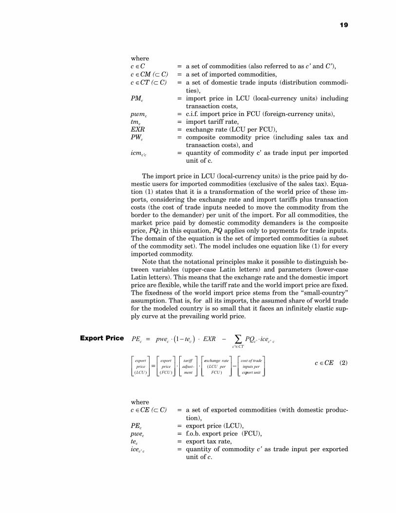
This chapter presents the mathematical model statement equation byequation. In its mathematical form, the CGE model is a system of simul-taneous, nonlinear equations. The model is squarethat is, the number ofequations is equal to the number of variables. In this class of models, thisis a necessary (but not a sufficient) condition for the existence of a uniquesolution. The chapter divides the equations into four blocks: prices, pro-duction and trade, institutions, and system constraints. New items (sets,parameters, and variables) are defined the first time that they appear inthe equations. Table 4 summarizes the notational principles. Parameterand variable names are chosen to facilitate interpretation; most impor-tantly, commodity and factor quantities start with q, commodity priceswith p, and factor prices with w.
PRICE BLOCK
Table 4Notational principles
Item Notation
Endogenous variables Upper-case Latin letters without a barExogenous variables Upper-case Latin letters with a barParameters Lower-case Latin letters (with or without a bar) or
lower-case Greek letters (with or without super-scripts)
Set indices Lower-case Latin letters as subscripts to variables andparameters
Notes: Exogenous variables are fixed in the basic model ver-sion but may be endogenous in versions with differenttreatments of macro- or factor-market closures.
Notes: For the specified closure rules, the choice for one of the three constraints does notconstrain the choice for the other two. MPS is marginal propensity to save.
The price system of the model is rich, primarily because of the assumedquality differences among commodities of different origins and destina-tions (exports, imports, and domestic outputs used domestically). Theprice block consists of equations in which endogenous model prices arelinked to other prices (endogenous or exogenous) and to nonprice modelvariables.
c ∈CM (1)
Import Price PM pwm tm EXR PQ icmc c c c c cc CT
importpriceLCU
= ⋅ +( ) ⋅ + ⋅
∈∑1 ' ''
( )
=
⋅
⋅importpriceFCU
tariffadjustment( )
-eexchange rate
LCU perFCU
()
+cost of tradeinputs perimpport unit
4.
18
wherec ∈C = a set of commodities (also referred to as c and C),c ∈CM (⊂ C) = a set of imported commodities,c ∈CT (⊂ C) = a set of domestic trade inputs (distribution commodi-
ties),PMc = import price in LCU (local-currency units) including
transaction costs,pwmc = c.i.f. import price in FCU (foreign-currency units),tmc = import tariff rate,EXR = exchange rate (LCU per FCU),PWc = composite commodity price (including sales tax and
transaction costs), andicmcc = quantity of commodity c as trade input per imported
unit of c.
The import price in LCU (local-currency units) is the price paid by do-mestic users for imported commodities (exclusive of the sales tax). Equa-tion (1) states that it is a transformation of the world price of these im-ports, considering the exchange rate and import tariffs plus transactioncosts (the cost of trade inputs needed to move the commodity from theborder to the demander) per unit of the import. For all commodities, themarket price paid by domestic commodity demanders is the compositeprice, PQ; in this equation, PQ applies only to payments for trade inputs.The domain of the equation is the set of imported commodities (a subsetof the commodity set). The model includes one equation like (1) for everyimported commodity.
Note that the notational principles make it possible to distinguish be-tween variables (upper-case Latin letters) and parameters (lower-caseLatin letters). This means that the exchange rate and the domestic importprice are flexible, while the tariff rate and the world import price are fixed.The fixedness of the world import price stems from the small-countryassumption. That is, for all its imports, the assumed share of world tradefor the modeled country is so small that it faces an infinitely elastic sup-ply curve at the prevailing world price.
c ∈CE (2)
wherec ∈CE (⊂ C) = a set of exported commodities (with domestic produc-
tion),PEc = export price (LCU),pwec = f.o.b. export price (FCU),tec = export tax rate,icec c = quantity of commodity c as trade input per exported
unit of c.
19
Export Price PE pwe te EXR PQ icec c c c c cc CT
priceLCU
= ⋅ −( ) ⋅ − ⋅
∈∑1 ' ''
( )
export
=
⋅
⋅export
-priceFCU
tariffadjustment( )
eexchange rateLCU per
FCU(
)
−cost of tradeinputs perexpport unit
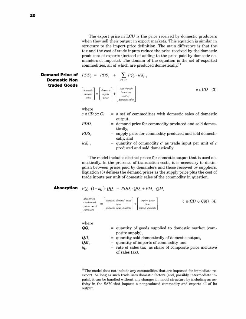
The export price in LCU is the price received by domestic producerswhen they sell their output in export markets. This equation is similar instructure to the import price definition. The main difference is that thetax and the cost of trade inputs reduce the price received by the domesticproducers of exports (instead of adding to the price paid by domestic de-manders of imports). The domain of the equation is the set of exportedcommodities, all of which are produced domestically.19
c ∈CD (3)
wherec ∈CD (⊂ C) = a set of commodities with domestic sales of domestic
output,PDDc = demand price for commodity produced and sold domes-
tically,PDSc = supply price for commodity produced and sold domesti-
cally, andicdc c = quantity of commodity c as trade input per unit of c
produced and sold domestically.
The model includes distinct prices for domestic output that is used do-mestically. In the presence of transaction costs, it is necessary to distin-guish between prices paid by demanders and those received by suppliers.Equation (3) defines the demand prices as the supply price plus the cost oftrade inputs per unit of domestic sales of the commodity in question.
c ∈(CD ∪ CM) (4)
whereQQc = quantity of goods supplied to domestic market (com-
posite supply),QDc = quantity sold domestically of domestic output,QMc = quantity of imports of commodity, andtqc = rate of sales tax (as share of composite price inclusive
of sales tax).
20
Demand Price of Domestic Nontraded Goods
PDD PDS PQ icdc c c c cc CT
domesticdemand
price
= + ⋅
=
∈∑ ' ''
dommesticsupplyprice
cost of tradeinputs per
unit of
+ddomestic sales
Absorption PQ tq QQ PDD QD PM QMc c c c c c c
absorptionat demand
prices n
⋅ −( ) ⋅ = ⋅ + ⋅1
(eet of
sales tax
domestic demand pricetimes
domestic sal)
=ees quantity
import pricetimes
import quantity
+
19The model does not include any commodities that are imported for immediate re-export. As long as such trade uses domestic factors (and, possibly, intermediate in-puts), it can be handled without any changes in model structure by including an ac-tivity in the SAM that imports a nonproduced commodity and exports all of its output.
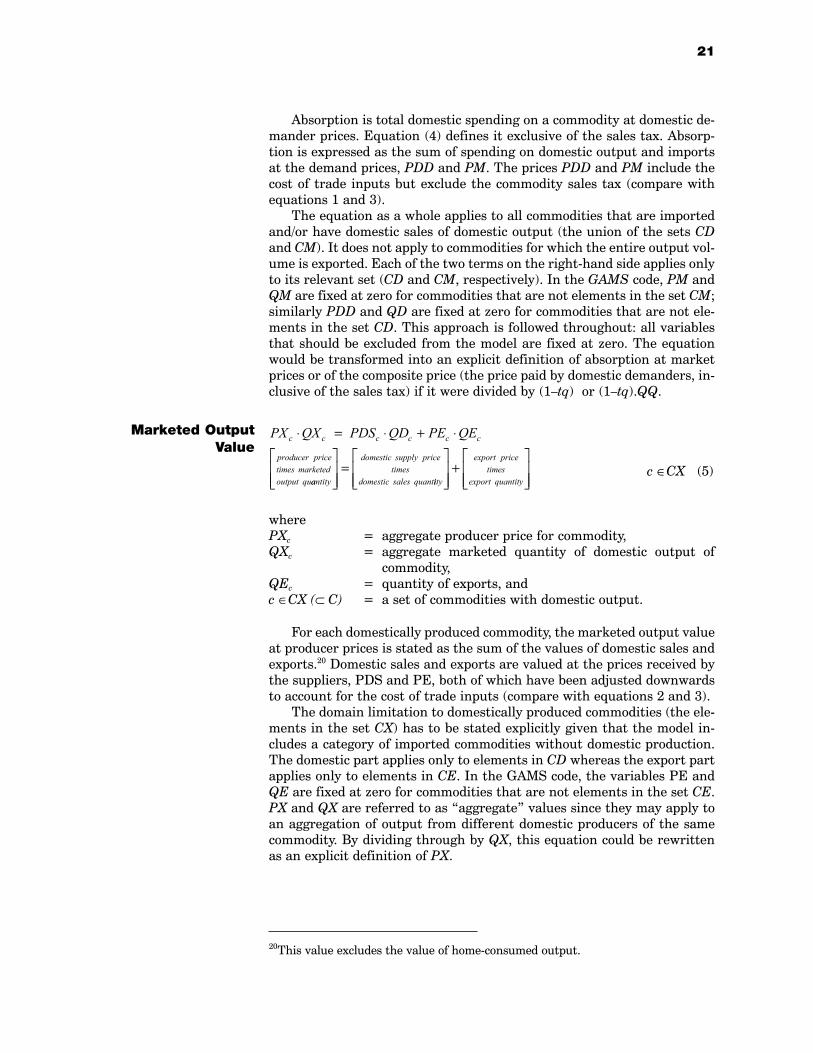
Absorption is total domestic spending on a commodity at domestic de-mander prices. Equation (4) defines it exclusive of the sales tax. Absorp-tion is expressed as the sum of spending on domestic output and importsat the demand prices, PDD and PM. The prices PDD and PM include thecost of trade inputs but exclude the commodity sales tax (compare withequations 1 and 3).
The equation as a whole applies to all commodities that are importedand/or have domestic sales of domestic output (the union of the sets CDand CM). It does not apply to commodities for which the entire output vol-ume is exported. Each of the two terms on the right-hand side applies onlyto its relevant set (CD and CM, respectively). In the GAMS code, PM andQM are fixed at zero for commodities that are not elements in the set CM;similarly PDD and QD are fixed at zero for commodities that are not ele-ments in the set CD. This approach is followed throughout: all variablesthat should be excluded from the model are fixed at zero. The equationwould be transformed into an explicit definition of absorption at marketprices or of the composite price (the price paid by domestic demanders, in-clusive of the sales tax) if it were divided by (1tq) or (1tq).QQ.
c ∈CX (5)
wherePXc = aggregate producer price for commodity,QXc = aggregate marketed quantity of domestic output of
commodity,QEc = quantity of exports, andc ∈CX (⊂ C) = a set of commodities with domestic output.
For each domestically produced commodity, the marketed output valueat producer prices is stated as the sum of the values of domestic sales andexports.20 Domestic sales and exports are valued at the prices received bythe suppliers, PDS and PE, both of which have been adjusted downwardsto account for the cost of trade inputs (compare with equations 2 and 3).
The domain limitation to domestically produced commodities (the ele-ments in the set CX) has to be stated explicitly given that the model in-cludes a category of imported commodities without domestic production.The domestic part applies only to elements in CD whereas the export partapplies only to elements in CE. In the GAMS code, the variables PE andQE are fixed at zero for commodities that are not elements in the set CE.PX and QX are referred to as aggregate values since they may apply toan aggregation of output from different domestic producers of the samecommodity. By dividing through by QX, this equation could be rewrittenas an explicit definition of PX.
21
20This value excludes the value of home-consumed output.
Marketed OutputValue
PX QX PDS QD PE QEc c c c c c
producer pricetimes marketedoutput qu
⋅ = ⋅ + ⋅
aantity
domestic pricetimes
domestic sales quant
=supply
iity
export pricetimes
export quantity
+
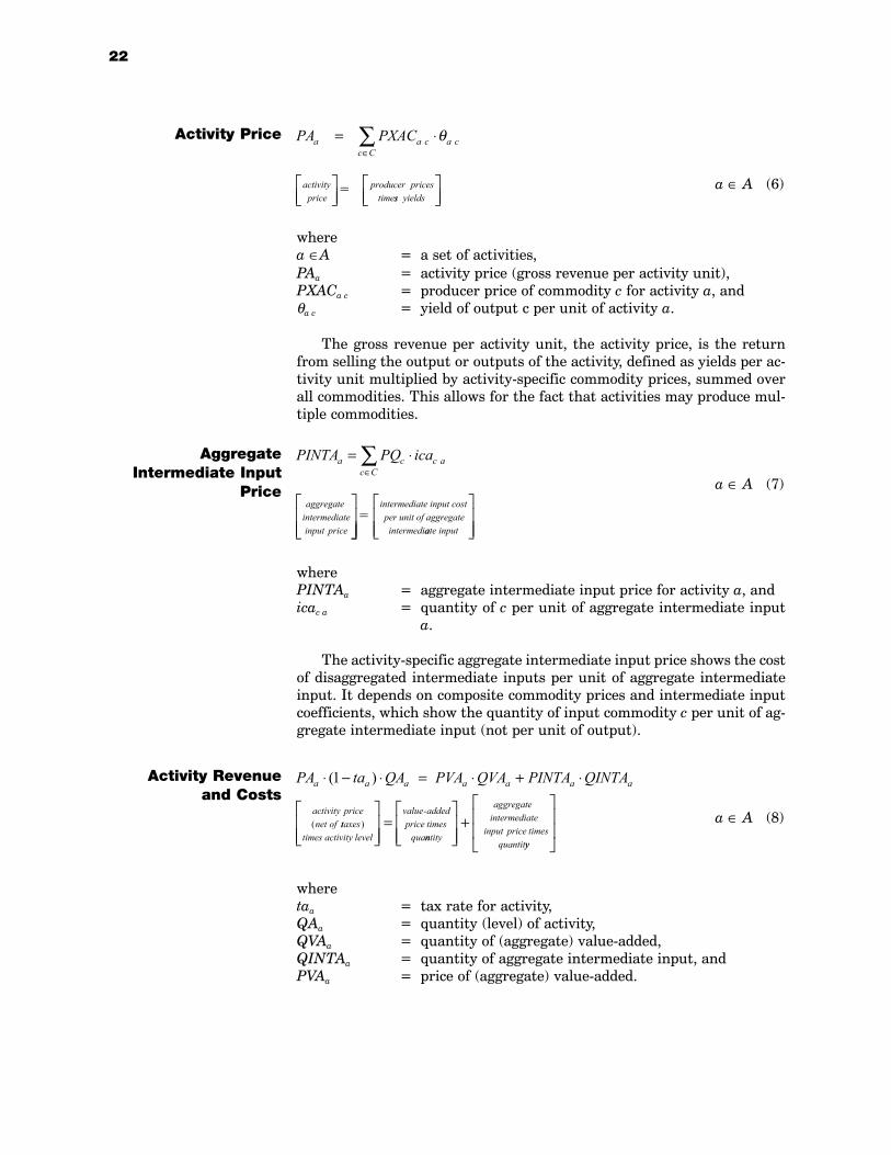
a ∈ A (6)
wherea ∈A = a set of activities,PAa = activity price (gross revenue per activity unit),PXACa c = producer price of commodity c for activity a, andθa c = yield of output c per unit of activity a.
The gross revenue per activity unit, the activity price, is the returnfrom selling the output or outputs of the activity, defined as yields per ac-tivity unit multiplied by activity-specific commodity prices, summed overall commodities. This allows for the fact that activities may produce mul-tiple commodities.
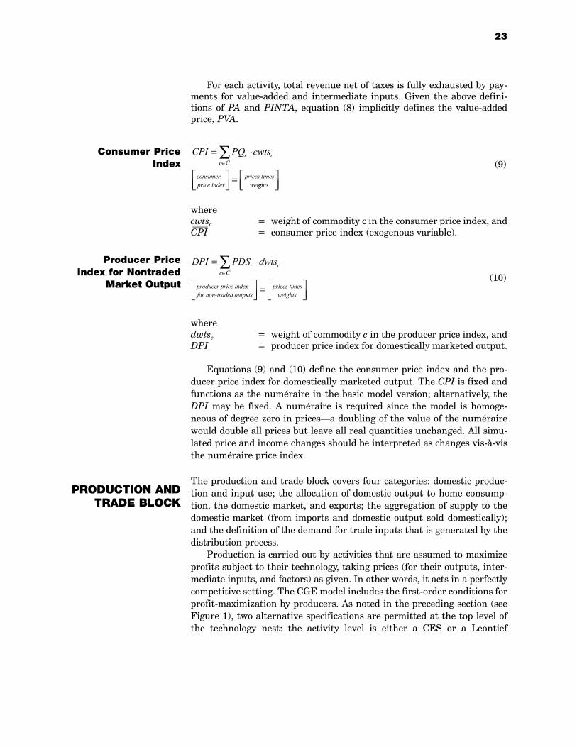
a ∈ A (7)
wherePINTAa = aggregate intermediate input price for activity a, andicac a = quantity of c per unit of aggregate intermediate input
a.
The activity-specific aggregate intermediate input price shows the costof disaggregated intermediate inputs per unit of aggregate intermediateinput. It depends on composite commodity prices and intermediate inputcoefficients, which show the quantity of input commodity c per unit of ag-gregate intermediate input (not per unit of output).
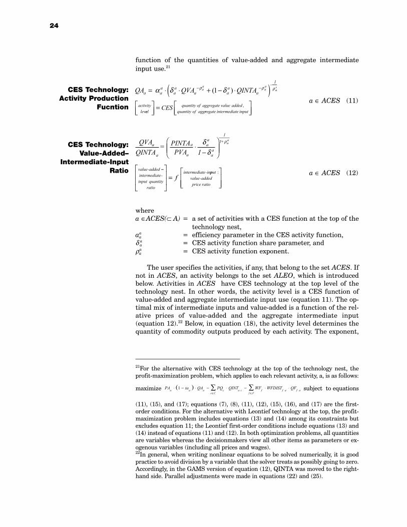
a ∈ A (8)
wheretaa = tax rate for activity,QAa = quantity (level) of activity,QVAa = quantity of (aggregate) value-added,QINTAa = quantity of aggregate intermediate input, and PVAa = price of (aggregate) value-added.
22
Activity Price PA PXACa a c a cc C
= ⋅
∈∑
activityprice
producer pricestime
=
θ
ss yields
Aggregate Intermediate Input
Price
Activity Revenue and Costs
PINTA PQ icaa c c ac C
= ⋅
∈∑
aggregate intermediateinput price
=intermediate input costper unit of aggregateintermediaate input
PA ta QA PVA QVA PINTA QINTAa a a a a a a
activity pricenet of
⋅ − ⋅ = ⋅ + ⋅( )
(
1
ttaxestimes activity level
value addedprice times
qua)
=-
nntity
aggregatemediate
input price timesquantit
+ inter
yy
For each activity, total revenue net of taxes is fully exhausted by pay-ments for value-added and intermediate inputs. Given the above defini-tions of PA and PINTA, equation (8) implicitly defines the value-addedprice, PVA.
(9)
wherecwtsc = weight of commodity c in the consumer price index, and CPI
= consumer price index (exogenous variable).
(10)
wheredwtsc = weight of commodity c in the producer price index, andDPI = producer price index for domestically marketed output.
Equations (9) and (10) define the consumer price index and the pro-ducer price index for domestically marketed output. The CPI is fixed andfunctions as the numéraire in the basic model version; alternatively, theDPI may be fixed. A numéraire is required since the model is homoge-neous of degree zero in pricesa doubling of the value of the numérairewould double all prices but leave all real quantities unchanged. All simu-lated price and income changes should be interpreted as changes vis-à-visthe numéraire price index.
The production and trade block covers four categories: domestic produc-tion and input use; the allocation of domestic output to home consump-tion, the domestic market, and exports; the aggregation of supply to thedomestic market (from imports and domestic output sold domestically);and the definition of the demand for trade inputs that is generated by thedistribution process.
Production is carried out by activities that are assumed to maximizeprofits subject to their technology, taking prices (for their outputs, inter-mediate inputs, and factors) as given. In other words, it acts in a perfectlycompetitive setting. The CGE model includes the first-order conditions forprofit-maximization by producers. As noted in the preceding section (seeFigure 1), two alternative specifications are permitted at the top level of the technology nest: the activity level is either a CES or a Leontief
23
CPI PQ cwtscc C
c= ⋅
=
∈∑
consumerprice index
prices timesweigghts
DPI PDS dwtscc C
c= ⋅∈∑
producer price index for non-traded outpuuts
prices timesweights
=
Consumer PriceIndex
Producer PriceIndex for Nontraded
Market Output
PRODUCTION ANDTRADE BLOCK
function of the quantities of value-added and aggregate intermediateinput use.21
a ∈ ACES (11)
a ∈ ACES (12)
wherea ∈ACES(⊂ A) = a set of activities with a CES function at the top of the
technology nest,aa
a = efficiency parameter in the CES activity function,δ a
a = CES activity function share parameter, andρa
a = CES activity function exponent.
The user specifies the activities, if any, that belong to the set ACES. Ifnot in ACES, an activity belongs to the set ALEO, which is introducedbelow. Activities in ACES have CES technology at the top level of thetechnology nest. In other words, the activity level is a CES function ofvalue-added and aggregate intermediate input use (equation 11). The op-timal mix of intermediate inputs and value-added is a function of the rel-ative prices of value-added and the aggregate intermediate input (equation 12).22 Below, in equation (18), the activity level determines thequantity of commodity outputs produced by each activity. The exponent,
24
21For the alternative with CES technology at the top of the technology nest, theprofit-maximization problem, which applies to each relevant activity, a, is as follows:
maximize subject to equations
(11), (15), and (17); equations (7), (8), (11), (12), (15), (16), and (17) are the first-order conditions. For the alternative with Leontief technology at the top, the profit-maximization problem includes equations (13) and (14) among its constraints butexcludes equation 11; the Leontief first-order conditions include equations (13) and(14) instead of equations (11) and (12). In both optimization problems, all quantitiesare variables whereas the decisionmakers view all other items as parameters or ex-ogenous variables (including all prices and wages).22In general, when writing nonlinear equations to be solved numerically, it is goodpractice to avoid division by a variable that the solver treats as possibly going to zero.Accordingly, in the GAMS version of equation (12), QINTA was moved to the right-hand side. Parallel adjustments were made in equations (22) and (25).
PA ta QA PQ QINT WF WFDIST QFa a a c a c f f a f af Fc C
⋅ − ⋅ − ⋅ − ⋅ ⋅( )∈∈∑∑1
CES Technology: Activity Production
Fucntion
CES Technology:Value-Added–
Intermediate-InputRatio
QA QVA QINTAa aa
aa
a aa
a
- 1
activitylev
aa
aa
aa= ⋅ ⋅ + − ⋅( )− −α δ δρ ρ ρ( )1
eelquantity of aggregate value added
quantity of aggCES
=
,rregate intermediate input
QVAQINTA
= PINTAPVA 1
a
a
a
a
aa
aa
11+
value added
aa
⋅−
δδ
ρ
- −−
=intermediateinput quantity
ratio
intermediate inf-
- pputvalue addedprice ratio
:-
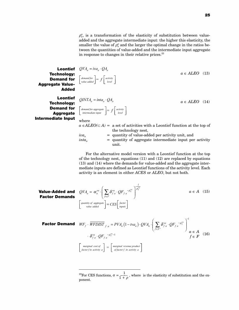
ρaa, is a transformation of the elasticity of substitution between value-
added and the aggregate intermediate input: the higher this elasticity, thesmaller the value of ρa
a and the larger the optimal change in the ratios be-tween the quantities of value-added and the intermediate input aggregatein response to changes in their relative prices.23
a ∈ ALEO (13)
a ∈ ALEO (14)
wherea ∈ALEO(⊂ A) = a set of activities with a Leontief function at the top of
the technology nest,ivaa = quantity of value-added per activity unit, andintaa = quantity of aggregate intermediate input per activity
unit.
For the alternative model version with a Leontief function at the topof the technology nest, equations (11) and (12) are replaced by equations(13) and (14) where the demands for value-added and the aggregate inter-mediate inputs are defined as Leontief functions of the activity level. Eachactivity is an element in either ACES or ALEO, but not both.
a ∈ A (15)
a ∈ A (16)f ∈ F
WF PVA tva QVA QFf a a a f ava
f af F
fava
⋅ = −( ) ⋅ ⋅ ⋅
−
∈∑WFDIST a 1 δ ρ
'
⋅ ⋅
−
− −
1
1δ ρf ava
f aQF ava
marginal cost offactor f in activity a
= marginal revenue productof factor f in activity a
25
Leontief Technology: Demand for
Aggregate Value-Added
Leontief Technology: Demand for
Aggregate Intermediate Input
Value-Added and Factor Demands
Factor Demand
QVA iva QAa a a= ⋅
demand for value added
activity level
= f
QINTA in a QAa a a= ⋅t
demand for aggregate intermediate input
= f activity level
QVA QFa ava
f ava
f af F
- 1
quantity of agg
ava a
va
= ⋅ ⋅
−
∈∑α δ ρ
ρ
rregatevalue added
factorinputs
CES
=
23For CES functions, σ = 1
1 + ρ
, where is the elasticity of substitution and the ex-ponent.
wheref ∈F(=F) = a set of factors,tvaa = rate of value-added tax for activity a,aa
va = efficiency parameter in the CES value-added function,δf
vaa = CES value-added function share parameter for factor f
in activity a,QFf a = quantity demanded of factor f from activity a,ρa
va = CES value-added function exponent, WFf = average price of factor, andWFDIST
fa = wage distortion factor for factor f in activity a (exoge-
nous variable).Equation (15) states that, for each activity, the quantity of value-added
is a CES function of disaggregated factor quantities. According to equa-tion (16), activities demand factors at the point where the marginal cost ofeach factor (defined on the left-hand side as the activity-specific factorprice) is equal to the marginal revenue product (net of intermediate inputcosts) of the factor. In the GAMS code, the domain of equation (16) is lim-ited to the factor-activity combinations that appear in the base-year SAM.Similar domain restrictions apply to other equations that are defined overmappings between multiple indices (for example, equation 17). The expo-nent, ρa
va, is a transformation of the elasticity of factor substitution: thehigher this elasticity, the smaller the value of ρa
va and the larger the opti-mal change in the ratios between different factor quantities in response tochanges in relative factor prices (compare with footnote 16).
The fact that the average factor price is an endogenous variable whilethe activity-specific wage-distortion factor is exogenous reflects thetreatment of factor markets in the basic model version (see equation 39below).
a ∈ A (17)c ∈ C
whereQINTc a = quantity of commodity c as intermediate input to activ-
ity a.
For each activity, the demand for disaggregated intermediate inputs isdetermined via a standard Leontief formulation as the level of aggregateintermediate input use times a fixed intermediate input coefficient.
a ∈ A (18)c ∈ CX
26
Disaggregated Intermediate Input
Demand
Commodity Production and
Allocation
QINT ica QINTAc a c a a
intermediate demand for commodity c f
= ⋅
rrom activity a
aggregate intermediate input qu= f
aantity for activity a
QXAC QHA QAa c a c hh H
a c a
marketed quantityof commodity
+ = ⋅∈∑ θ
c from activity a
household home consumption
of c
+
oommodity c from activity a
productionof commodity
= c from activity a
whereQXACa c = marketed output quantity of commodity c from activity
a, andQHAa c h = quantity of household home consumption of commodity
c from activity a for household h.
On the right-hand side, production quantities, disaggregated by activ-ity, are defined as yields times activity levels. On the left-hand side, thesequantities are allocated to market sales and home consumption. Note thatthis equation permits (i) any commodity to be produced by one or more ac-tivities and (ii) any activity to produce one or more commodities.24
c ∈ CX (19)
whereac
ac = shift parameter for domestic commodity aggregationfunction,
δa cac = share parameter for domestic commodity aggregation
function, andρc
ac = domestic commodity aggregation function exponent.
a ∈ A (20)c ∈ CX
Aggregate marketed production of any commodity is defined as a CESaggregate of the marketed output levels of the different activities produc-ing the commodity (equation 19). The optimal quantity of the commodityfrom each activity source is inversely related to the activity-specific price(equation 20). QX appears as the output, sold at the price, PX, and pro-duced with the inputs, QXAC, that are purchased at the prices, PXAC.
More specifically, the choice between commodities from differentsources is cast as an optimization problem. Equations (19) and (20) are the
27
Output AggregationFunction
First-Order Condition for Output
Aggregation Function
QX QXACc cac
a cac
a ca A
cac c
ac
= ⋅ ⋅
−
∈
−−
∑α δ ρρ
aggregatem
11
aarketedproduction of commodity c
activity-spec
= CES
iific marketed
production ofcommodity c
PXAC = PX QX QXAC a c c ca A
a cac
a c a ccac
⋅ ⋅
⋅
∈
−∑−
'
δ δρ1
aaca cQXAC c
ac⋅ − −
marginal cost of com-modity c from activ
ρ 1
iity amarginal revenue product ofcommodity c from a
=
cctivity a
24In the SAM, home consumption is represented by payments from households to ac-tivities. For the case of home consumption out of activities with multiple outputs, itis necessary to complement the information in the SAM with data on the allocationof consumption across the different activity outputs.
c
c
c
c
ct
ct
QEQD
= PEPDS
1 ct
⋅−
−δδ
ρ1
1
export-domesticsuppply ratio
export-domesticprice ratio
= f
first-order conditions for maximizing profits from selling the aggregateoutput, QX, at the price, PX, subject to the aggregation function and thedisaggregated commodity prices, PXAC. A decline in the price, PXAC, ofone activity relative to others would shift demand in its favor without to-tally eliminating demand for other, higher-price sources. The degree ofsubstitutability between different producers depends on the value of ρc
ac,which is a transformation of the elasticity of substitution (compare withfootnote 16). Its values, and those of the elasticity, are restricted to assurethat the corresponding isoquant is convex to the origin. In terms of pro-duction economics, this is equivalent to a diminishing technical rate ofsubstitution.
It should be noted that, for the case where there is a single producerof a given commodity, the value of the share parameter, δa c
ac, would beunity and, as a result, QXAC = QX and PXAC = PX, irrespective of thevalues for the elasticity and the exponent.
c ∈(CE ∩ CD) (21)
whereac
t = a CET function shift parameter,δc
t = a CET function share parameter, andρc
t = a CET function exponent.
Equations (21) and (22) address the allocation of marketed domesticoutput, defined in equation (19), to two alternative destinations: domesticsales and exports. Equation (21) reflects the assumption of imperfecttransformability between these two destinations. The CET function,which applies to commodities that are both exported and sold domesti-cally, is identical to a CES function except for negative elasticities of sub-stitution. The elasticity of transformation between the two destinations isa transformation of ρ t
c , for which the lower limit is one. The values are re-stricted to assure that the isoquant corresponding to the output transfor-mation function is concave to the origin.25
c ∈(CE ∩ CD) (22)
28
Output Transformation(CET) Function
Export-DomesticSupply Ratio
c ct
ct
c ct
cQX = QE + QDct
ct
ct
α δ δρ ρ ρ⋅ ⋅ − ⋅( )(11
)
aggregate marketteddomestic output
export quantity, domesticsales o
=
CETff domestic output
25For CET functions, Ω = 1
1 + ρ
, where is the elasticity of transformation and p the
exponent. As Ω varies from zero to infinity, the value of ρ tc varies from infinity to one.
In equation (22), as ptc approaches one from above, the elasticity of the QE-QD ratiowith respect to changes in the PE-PDD ratio increases.
c c c
aggregatemarketed
domestic output
domes
QX = QD QE+
=ttic market
sales of domesticoutput for
c (CD CEN)][
∈ ∩
+ eexports c (CE CDN)]
[ for∈ ∩
Equation (22) defines the optimal mix between exports and domesticsales. Equations (5), (21), and (22) constitute the first-order conditions formaximization of producer revenues given the two prices and subject to theCET function and a fixed quantity of domestic output. Note that equation(22) assures that an increase in the export-domestic price ratio generatesan increase in the export-domestic supply ratio (that is, a shift toward thedestination that offers the higher return).
c ∈(CD ∩ CEN) ∪ (CE ∩ CDN) (23)
wherec ∈CEN (⊂ C) = non-exported commodities (complement of CE), andc ∈CDN (⊂ C) = commodities without domestic market sales of domes-
tic output (complement of CD).
This equation replaces the CET function for domestically producedcommodities that do not have both exports and domestic sales. It allocatesthe entire output volume to one of these two destinations.
c ∈(CM ∩ CD) (24)
whereac
q = an Armington function shift parameter,δc
q = an Armington function share parameter, andρc
q = an Armington function exponent.
Imperfect substitutability between imports and domestic output solddomestically is captured by a CES aggregation function in which the com-posite commodity that is supplied domestically is produced by domesticand imported commodities entering this function as inputs. When thedomain of this function is limited to commodities that are both importedand produced domestically, it is often called an Armington function,named after the originator of the idea of using a CES function for this pur-pose. The elasticity of substitution between commodities from these twosources is a transformation of for which the lower limit is minus one(compare with footnote 16).
c ∈(CM ∩ CD) (25)
29
Output Transformation for Domestically Sold
Outputs Without Exports and for Exports Without Domestic Sales
Composite Supply(Armington)
Function
Import-Domestic Demand Ratio
c cq
cq
c-
cq
c-
- 1
QQ = QM + (1 ) QDcq
cq
cqα δ δρ ρ ρ⋅ ⋅ − ⋅( )
compositesuppply
import quantity, domesticuse of domestic output
= f
Equation (25) defines the optimal mix between imports and domesticoutput. Its domain is thus limited to imports with domestic production.Note that the equation assures that an increase in the domestic-importprice ratio generates an increase in the import-domestic demand ratio(that is, a shift away from the source that becomes more expensive).26 To-gether, equations (4), (24), and (25) constitute the first-order conditionsfor cost-minimization given the two prices and subject to the Armingtonfunction and a fixed quantity of the composite commodity.
c ∈(CD ∩ CMN) ∪ (CM ∩ CDN) (26)
wherec ∈CMN (⊂ C) = a set of non-imported commodities.
The Armington function is replaced by equation (26) for the union ofcommodities that have either imports or domestic sales of domestic outputbut not both. For any commodity in this category, it imposes equality be-tween composite supply and one of the variables on the right-hand side.
c ∈CT (27)
whereQTc = quantity of commodity demanded as transactions serv-
ice input.
Total demand for trade inputs is the sum of the demands for these in-puts that are generated by imports (from moving commodities from theborder to domestic demanders), exports (from moving commodities fromdomestic producers to the border), and domestic market sales (from mov-ing commodities from domestic producers to domestic demanders). In allthree cases, fixed quantities of one or more transactions service inputs arerequired per unit of the traded commodity.
c c c
compositedomestic use of
marketed
QQ = QD QM+
=supply
ddomestic
c CMN)]
coutput for
CD
imports forC[
(
[(
∈ ∩∈
+MM ∩
CDN)]
c c c c c c c c c cc C
QT = icm QM ice QE icd QD
demand
' ' ' ' ' '' '
⋅ + ⋅ + ⋅( )∈∑
fortransactions
services
sum of demandsfor import=
ss, exports, and domestic sales
30
Composite Supplyfor Non-importedOutputs and Non-produced Imports
Demand for Transactions
Services
26See footnote 16 for the definition of the elasticity of substitution. In equation (25),as the value of ρq
c approaches minus one from above, the elasticity of the import-domestic demand ratio with respect to changes in the PDD-PM ratio increases.
YI = YIF TRII trnsfr CPI trnsfri i f i i i govi INSDNG
i r + + ⋅ +∈∑ '
' 'oow
f FEXR⋅
∈∑
income of institution i
factorincome
=
+
transfersfrom other domestic
non-governmentinstitutions
+ +transfers
fromgovernment
transfers from RoWW
f ∈F (28)
whereYFf = income of factor f.
i ∈INSD (29)f ∈F
where i ∈INS = a set of institutions (domestic and rest of the world),i ∈INSD(⊂ INS) = a set of domestic institutions,YIFi f = income to domestic institution i from factor f,shifi f = share of domestic institution i in income of factor f,tff = direct tax rate for factor f, andtrnsfri f = transfer from factor f to institution i.
Equation (28) defines the total income of each factor. In equation (29),this income is split among domestic institutions in fixed shares after pay-ment of direct factor taxes and transfers to the rest of the world.27 The lat-ter are fixed in foreign currency and transformed into domestic currencyby multiplying by the exchange rate. This equation makes reference to theset of domestic institutions (households, enterprises, and the govern-ment), a subset of the set of institutions, which also includes the rest ofworld.
i ∈INSDNG (30)
wherei ∈INSDNG(=INSDNG ⊂ INSD)
= a set of domestic nongovernment institutions,YIi = income of institution i (in the set INSDNG), andTRIIii = transfers from institution i to i (both in the set INS-
DNG).
31
INSTITUTIONBLOCK
Factor Income
Institutional FactorIncomes
YF = WF QFf fa A
f af∈∑ ⋅ ⋅
WFDIST
=
a
income of factor f
sum of activity payments(activity-specific wages times employyment levels)
YIF = tf YF trnsfr EXRi f f f row i f f
income of i
shif ⋅ −( ) ⋅ − ⋅
1
nnstitution i from factor f
share of incomeof fact=
oor f toinstitution i
income of factor f(net of t
⋅ aax and transfer to RoW)
Income of domestic,Nongovernment
Institutions
27To assure that the total factor income is distributed, it is necessary that Σi∈INSD
shiftif = 1.
Domestic nongovernment institutions form a subset of the set of do-mestic institutions. The total income of any domestic nongovernment in-stitution is the sum of factor incomes (defined in equation 29), transfersfrom other domestic nongovernment institutions (defined below in equa-tion 31), transfers from the government (indexed to the CPI), and trans-fers from the rest of the world.28
i ∈INSDNG (31)i ∈INSDNG
whereshiiii = share of net income of i to i (i∈INSDNG; i∈INS-
DNG),MPSi = marginal propensity to save for domestic nongovern-
ment institution (exogenous variable), andTINSi = direct tax rate for institution i (i ∈INSDNG).
Transfers between domestic nongovernment institutions are paid asfixed shares of the total institutional incomes net of direct taxes and sav-ings. The values of MPS and TINS are defined in separate equations, dis-cussed below.
h ∈H (32)
wherei ∈H(⊂ INSDNG)
= a set of households, andEHh = household consumption expenditures.
Among the domestic nongovernment institutions, only households de-mand commodities. In equation (32), the total value of consumptionspending is defined as the income that remains after direct taxes, savings,and transfers to other domestic nongovernment institutions.
32
Infra-InstitutionalTransfers
Household Consumption Expenditures
TRII = shii MPS TINS YIi i i i i i i
transfer from
' ' ' ' '⋅ −( ) ⋅ −( ) ⋅1 1
iinstitution i' to i
share of net income of institut=
iion i'transfered to i
income of institution i', net
⋅ of savings and direct taxes
EH = shii MPS TINS YIh i hi INSDNG
h h h1 1 1−
⋅ −( ) ⋅ −( ) ⋅
∈∑
houusehold income disposable for consumption
househo=
lld income, net of direct taxes, savings, and transfers to
other non-government institutions
28The fact that government transfers are indexed to the CPI makes the model homo-geneous of degree zero in prices. This indexing influences the results when the DPI isthe model numéraire. If the CPI is the numéraire, it has no effect.
PQ QH = PQ EH PQ PXACc c h c c hm
c hm
h c c hm
c Ca c⋅ ⋅ + ⋅ − ⋅ − ⋅
∈∑ γ β γ γ' ''
' aa c hh
c Ca A
household consumptionspending on
''∈∈∑∑
mmarket commodity c
ftotal household consumption
sp=
eending, market price of c, and other commodity prices (marrket and home)
c ∈C (33)h∈H
whereQHc h = quantity of consumption of marketed commodity c for
household h,γ m
c h = subsistence consumption of marketed commodity c forhousehold h,
γ ha c h = subsistence consumption of home commodity c from ac-
tivity a for household h, andβ m
c h = marginal share of consumption spending on marketedcommodity c for household h.
a ∈Ac ∈C (34)h ∈H
whereβ h
a c h = marginal share of consumption spending on home com-modity c from activity a for household h.
It is assumed that each household maximizes a StoneGeary utilityfunction subject to a consumption expenditure constraint. The resultingfirst-order conditions, equations (33) and (34), are referred to as LES (lin-ear expenditure system) functions since spending on individual commodi-ties is a linear function of total consumption spending, EH. Two functionsare needed since household consumption is for two types of commodities:(i) consumption of marketed commodities (purchased at market prices;equation 33) and (ii) consumption of home production (valued at their op-portunity cost, the activity-specific producer price not including market-ing costs; equation 34). Explicit demand functions may be derived by di-viding both sides of each equation by the relevant price.
c ∈C (35)
33
Household Consumption Spending on
Marketed Commodities
Household Consumption Spending on
Home Commodities
PXAC QHA = PXAC
EH PQ
a c a c h a c a c hh
a c hh
h c c hm
c
⋅ ⋅ +
⋅ − ⋅
γ β
γ' '''
' ''∈ ∈∈
∑ ∑∑− ⋅
Ca c a c h
h
c Ca APXAC
household consumpt
γ
iionspending on home commodity
c from activity af
t=
ootal household consumption spending, producer price, and oother
commodity prices (market and home)
Investment Demand QINV = IADJ qinvc c⋅
fixed investmentdemand forcommodity c
=adjustment factor
timesbase-year
investment fixed
whereQINVc = quantity of fixed investment demand for commodity,IADJ
= investment adjustment factor (exogenous variable),and
qinvc
= base-year quantity of fixed investment demand.
Fixed investment demand is defined as the base-year quantity multi-plied by an adjustment factor. For the basic model version, the adjustmentfactor is exogenous, in effect also making the investment quantity exogenous. Inventory investment is also included in the model, but istreated as an exogenous demand (see equation 40 below).
c ∈C (36)
whereQGc = government consumption demand for commodity,GADJ
= government consumption adjustment factor (exogenous variable), and
qgc = base-year quantity of government demand.
Similarly, government consumption demand, in which the main com-ponent tends to be the services provided by the government labor force, isalso defined as the base-year quantity multiplied by an adjustment factor.This factor is also exogenous and, hence, the quantity of government con-sumption is fixed.
(37)
whereYG = government revenue.
34
Government Consumption
Demand
Government Revenue
QG = GADJ qgc c⋅
government consumptiondemand forcommodity c
=
adjustment factortimes
base-year governmentconsumption
YG TINS YI tf YF tva PVA QVA
ta
i ii INSDNG
f ff F
a a aa A
a a
= ⋅ + ⋅ + ⋅ ⋅
+ ⋅∈ ∈ ∈∑ ∑ ∑
PPA QA tm pwm QM EXR te pwe QE EXR
tq
aa A
c c cc CM
c c cc CE
⋅ + ⋅ ⋅ ⋅ + ⋅ ⋅ ⋅
+∈ ∈ ∈∑ ∑ ∑
cc c c gov ff F
gov rowc C
PQ QQ YIF trnsfr EXR⋅ ⋅ + + ⋅∈∈∑∑
governmentrevenue
direct taxes from
institutions=
+ +
direct taxesfrom
factors
value-added
tax
+ + +activitytax
importtariffs
exporttaxes
+ + +sales
taxfactor
income
transfersfromRoW
Total government revenue is the sum of revenues from taxes, factors,and transfers from the rest of the world.
(38)
whereEG = government expenditures.
Total government spending is the sum of government spending onconsumption and transfers.
f ∈F (39)
whereQFS
f = quantity supplied of factor (exogenous variable).
Equation (39) imposes equality between the total quantity demandedand the total quantity supplied for each factor. In the basic model version,all demand variables are flexible while the supply variable is fixed. Thefactor wage, WFf , is the equilibrating variable that assures that this equa-tion is satisfied: an increase in WFf raises the wage paid by each activity, WFf
. WFDIST
f a , which is inversely related to the quantities of factor de-
mand, QFf a. All factors are mobile between the demanding activities. Two other factor-market closures are programmed in the GAMS ver-
sion. To specify the case with unemployment at a given wage for a factor,the supply variable for the factor is unfixed (QFSf) while its economywidewage is fixed (WF
f). The model remains square (one endogenous variable
is added but another is removed). Each activity is free to employ the quan-tity it desires (QFf a) at a fixed wage (WF
f . WFDIST
f a). The free supply
variable, QFSf , records the total employment level. Alternatively, to specify the case of a fully segmented factor market
with fixed factor demands (for example, short-run fixity of nonagriculturalcapital use), the variables for factor demand and the economywide wageare fixed (written
QFf a and WF
f) while the variables for supply and wage
distortions are unfixed (written QFSf and WFDISTf a). The model againremains squarethat is, the economywide wage variable and a set of ac-tivity-specific factor-demand variables are fixed while the supply variableand a set of activity-specific wage-distortion variables are unfixed.
35
Government Expenditure
EG PQ QG trnsfr CPIc c i govi INSDNGc C
= ⋅ + ⋅
∈∈∑∑
governmentspending
= +governmentconsumption
transfers to domesticnonn-government
institutions
QF QFSf a fa A
demand forfactor f
offactor f
supply
=
=
∈∑
SYSTEM CONSTRAINT
BLOCK
Factor Markets
pwm QM trnsfr pwe QE trnsfrcc CM
c row ff F
cc CE
c i rowi I
⋅ + = ⋅ +∈ ∈ ∈ ∈∑ ∑ ∑
NNSDFSAV∑ +
+
importspending
factor transfers to RoW
= +export revenue
institutional transfersfrom RoW
+ foreignsavings
Activity-specific wages, WFf . WFDISTf a , vary to assure that the fixed ac-
tivity-specific employment level, QFf a , is consistent with profit-maxi-
mization (compare with equation 16). Also for this formulation, the en-dogenous aggregate factor supply variable merely records the total em-ployment level.
c ∈C (40)
whereqdstc = quantity of stock change.
Equation (40) imposes equality between quantities supplied (fromequations 24, 25, and 26) and demanded of the composite commodity. Thedemand side includes endogenous terms (from equations 17, 27, 33, 35,and 36) and a new exogenous term for stock change. Among the endoge-nous terms, QG and QINV are fixed in the basic model version (comparewith equations 35 and 36). The composite commodity supply, QQ, drivesdemands for domestic marketed output, QD, and imports, QM. The market-clearing variables are the quantities of import supply, for the im-port side, and the two interrelated domestic prices, PDD and PDS, for do-mestic market output.
(41)
whereFSAV
= foreign savings (FCU) (exogenous variable).
The current-account balance, which is expressed in foreign currency,imposes equality between the countrys spending and its earning of for-eign exchange. For the basic model version, foreign savings is fixed; the(real) exchange rate (EXR) serves the role of equilibrating variable to thecurrent-account balance. The fact that all items except imports and ex-ports are fixed means that, in effect, the trade deficit also is fixed. Alter-natively, the exchange rate may be fixed and foreign savings unfixed. Inthis case, the trade deficit is free to vary.
36
Composite Commodity Markets
compositesupply
intermediateuse
householdconsu
+
=
mmption
governmentconsumption
fixedinvestment
+
+
+ +stockchange
tradeinput use
QQ QINT QH QG QINV qdst QTc c aa A
c hh H
c c c c= + + + + +∈ ∈∑ ∑
Current-AccountBalance for the
Rest of the World, inForeign Currency
(42)
whereGSAV = government savings.
The government balance imposes equality between current govern-ment revenue and the sum of current government expenditures (not in-cluding government investment) and savings. Savings may be negative.The alternative mechanisms for maintaining this balance are associatedwith equation (43).
i ∈INSDNG (43)
whereTINSi = rate of direct tax on domestic institutions i,tinsi = exogenous direct tax rate for domestic institution i,TINSADJ
= direct tax scaling factor (= 0 for base; exogenous vari-
able), tins01i = 01 parameter with 1 for institutions with potentially
flexed direct tax rates, andDTINSi
= change in domestic institution tax share (= 0 for base;
exogenous variable).
Equation (43) defines the direct tax rates of domestic nongovernmentinstitutions. For the basic model version, all variables on the right-handside are fixed, in effect fixing the values for the direct tax rate variable forall institutions. In this setting, government savings is the endogenousvariable that clears the government balance.
In the GAMS implementation of the standard model, two alternativeclosure rules are coded for the government balance (see MacroeconomicBalances in Chapter 3). For both alternatives, government savings isfixed. In the first case, DTINS is the flexible variable that clears the gov-ernment balance by scaling the base-year tax rates of each tax-paying in-stitution. In this setting, the rates will change by a uniform number of(percentage) points for all institutions with a value of 1 for the parametertins01 (that is, for all institutions with potentially flexed direct tax rates).Hence, the initial tax rate has no impact on the rate change. In the secondcase, TINSADJ becomes a variable while DTINS is fixed. For this closure,the changes in TINS are relatively large for institutions with relativelylarge base-year rates (if they have a value of 1 for tins01).
37
YG EG GSAVgovernment
revenuegovernment
= +
= expenditures
+
governmentsavings
TINS tins TINSADJ tins DTINS tii i i
direct
= ⋅ + ⋅( ) + ⋅1 01
tax ratte
institution i
base rate adjustedfor scalinfor
= gg for selected institutions
point change for sele
+ cctedinstitutions
Government Balance
Direct InstitutionalTax Rates
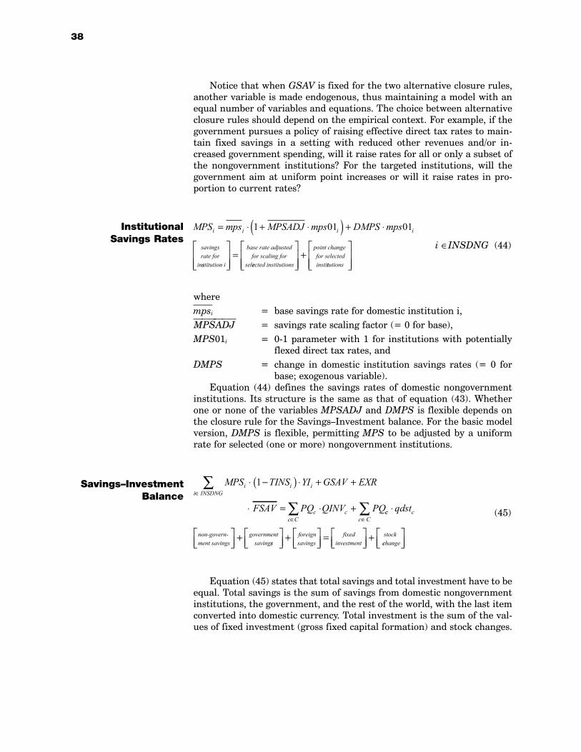
Notice that when GSAV is fixed for the two alternative closure rules,another variable is made endogenous, thus maintaining a model with anequal number of variables and equations. The choice between alternativeclosure rules should depend on the empirical context. For example, if thegovernment pursues a policy of raising effective direct tax rates to main-tain fixed savings in a setting with reduced other revenues and/or in-creased government spending, will it raise rates for all or only a subset ofthe nongovernment institutions? For the targeted institutions, will thegovernment aim at uniform point increases or will it raise rates in pro-portion to current rates?
i ∈INSDNG (44)
wherempsi = base savings rate for domestic institution i,MPSADJ
= savings rate scaling factor (= 0 for base),
MPS01i = 0-1 parameter with 1 for institutions with potentiallyflexed direct tax rates, and
DMPS = change in domestic institution savings rates (= 0 forbase; exogenous variable).
Equation (44) defines the savings rates of domestic nongovernmentinstitutions. Its structure is the same as that of equation (43). Whetherone or none of the variables MPSADJ and DMPS is flexible depends onthe closure rule for the SavingsInvestment balance. For the basic modelversion, DMPS is flexible, permitting MPS to be adjusted by a uniformrate for selected (one or more) nongovernment institutions.
(45)
Equation (45) states that total savings and total investment have to beequal. Total savings is the sum of savings from domestic nongovernmentinstitutions, the government, and the rest of the world, with the last itemconverted into domestic currency. Total investment is the sum of the val-ues of fixed investment (gross fixed capital formation) and stock changes.
38
Institutional Savings Rates
MPS mps MPSADJ mps DMPS mpsi i i i
savingsfor
= ⋅ + ⋅( ) + ⋅1 01 01
rate
insstitution i
base rate adjustedfor scaling for
sel
=eected institutions
point change for selectedinsti
+ttutions
Savings–InvestmentBalance
MPS TINS YI GSAV EXR
FSAV PQ QINV PQ
i ii INSDNG
i
cc C
c
⋅ −( ) ⋅ + +
⋅ = ⋅ +∈
∈
∑
∑
1
cc cc C
qdst⋅
+
∈∑
non-govern-ment savings
governmentsavingss
foreignsavings
fixedinvestment
stock
+
=
+cchange
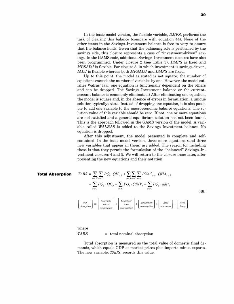
In the basic model version, the flexible variable, DMPS, performs thetask of clearing this balance (compare with equation 44). None of theother items in the SavingsInvestment balance is free to vary to assurethat the balance holds. Given that the balancing role is performed by thesavings side, this closure represents a case of investment-driven sav-ings. In the GAMS code, additional SavingsInvestment closures have alsobeen programmed. Under closure 2 (see Table 3), DMPS is fixed and MPSADJ is flexible. For closure 3, in which investment is savings-driven,IADJ is flexible whereas both MPSADJ and DMPS are fixed.
Up to this point, the model as stated is not square; the number ofequations exceeds the number of variables by one. However, the model sat-isfies Walras law: one equation is functionally dependent on the othersand can be dropped. The SavingsInvestment balance or the current-account balance is commonly eliminated.) After eliminating one equation,the model is square and, in the absence of errors in formulation, a uniquesolution typically exists. Instead of dropping one equation, it is also possi-ble to add one variable to the macroeconomic balance equations. The so-lution value of this variable should be zero. If not, one or more equationsare not satisfied and a general equilibrium solution has not been found.This is the approach followed in the GAMS version of the model. A vari-able called WALRAS is added to the SavingsInvestment balance. Noequation is dropped.
After this adjustment, the model presented is complete and self-contained. In the basic model version, three more equations (and threenew variables that appear in them) are added. The reason for includingthese is that they permit the formulation of the balanced SavingsIn-vestment closures 4 and 5. We will return to the closure issue later, afterpresenting the new equations and their notation.
(46)
whereTABS = total nominal absorption.
Total absorption is measured as the total value of domestic final de-mands, which equals GDP at market prices plus imports minus exports.The new variable, TABS, records this value.
39
Total Absorption TABS PQ QH PXAC QHA
PQ QG
cc Ch H
c h a c a c hh Hc Ca A
c
= ⋅ + ⋅
+ ⋅∈∈ ∈∈∈∑∑ ∑∑∑
ccc C
c cc C
c cc C
PQ QINV PQ qdst∈ ∈ ∈∑ ∑ ∑+ ⋅ + ⋅
total absorption
householdmarket
consumption
=
+hhousehold
homeconsumption
governmentconsumption
+
+
+
fixedinvestment
stockchange
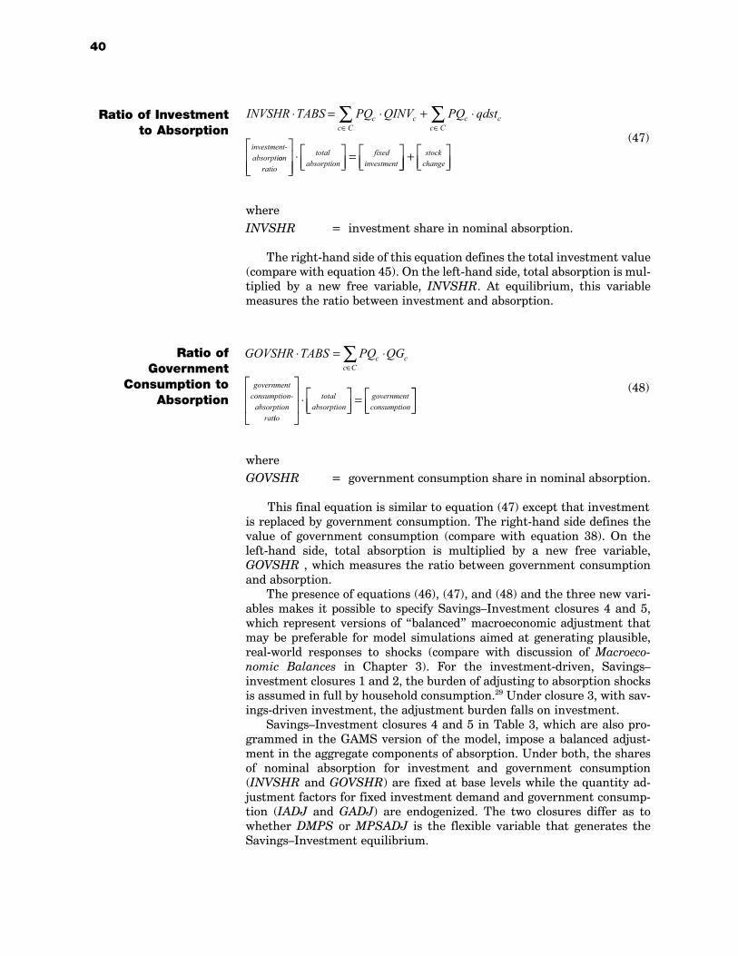
(47)
whereINVSHR = investment share in nominal absorption.
The right-hand side of this equation defines the total investment value(compare with equation 45). On the left-hand side, total absorption is mul-tiplied by a new free variable, INVSHR. At equilibrium, this variablemeasures the ratio between investment and absorption.
(48)
whereGOVSHR = government consumption share in nominal absorption.
This final equation is similar to equation (47) except that investmentis replaced by government consumption. The right-hand side defines thevalue of government consumption (compare with equation 38). On theleft-hand side, total absorption is multiplied by a new free variable, GOVSHR , which measures the ratio between government consumptionand absorption.
The presence of equations (46), (47), and (48) and the three new vari-ables makes it possible to specify SavingsInvestment closures 4 and 5,which represent versions of balanced macroeconomic adjustment thatmay be preferable for model simulations aimed at generating plausible,real-world responses to shocks (compare with discussion of Macroeco-nomic Balances in Chapter 3). For the investment-driven, Savingsinvestment closures 1 and 2, the burden of adjusting to absorption shocksis assumed in full by household consumption.29 Under closure 3, with sav-ings-driven investment, the adjustment burden falls on investment.
SavingsInvestment closures 4 and 5 in Table 3, which are also pro-grammed in the GAMS version of the model, impose a balanced adjust-ment in the aggregate components of absorption. Under both, the sharesof nominal absorption for investment and government consumption (INVSHR and GOVSHR) are fixed at base levels while the quantity ad-justment factors for fixed investment demand and government consump-tion (IADJ and GADJ) are endogenized. The two closures differ as towhether DMPS or MPSADJ is the flexible variable that generates theSavingsInvestment equilibrium.
40
Ratio of Investmentto Absorption
Ratio of Government
Consumption to Absorption
INVSHR TABS PQ QINV PQ qdstc cc C
c cc C
⋅ = ⋅ + ⋅∈ ∈∑ ∑
investment-absorptioon
ratio
totalabsorption
fixedinvestment
⋅
=
+
stockchange
GOVSHR TABS PQ QGcc C
c⋅ = ⋅∈∑
governmentconsumption-
absorptionratiio
totalabsorption
governmentconsumption
⋅
=
Under these two closures, any change in total absorption would, innominal terms, be spread evenly across all three components of absorp-tion; given the shares for investment and government consumption, theshare for household consumption is implicitly defined. Adjustments in thenongovernment savings value clear the savings- investment balance. Themagnitude of the savings adjustment, which is influenced by changes ininvestment and government consumption (for the latter via changes ingovernment savings), determines the availability of resources for house-hold consumption.
41
29However, for simulations with single-period models (like the current model) aimed atexploring welfare impacts of exogenous shocks, the SavingsInvestment closure 1 or 2is often preferable since the model is unable to capture future welfare changes associ-ated with current changes in investment (compare with the Macroeconomic Balancesdiscussion in Chapter 3).
THE STANDARD MODEL IN GAMS
The GAMS input files contained in the CD-ROM that accompanies thismanual include country data files that enable the user to conduct simula-tions with the standard model using data for a selected country. It is alsostraightforward to apply this modeling system to alternative country datasets generated by the user. This chapter provides a brief guide to theGAMS files and suggestions on how to use this modeling system. The filesthemselves include additional explanatory comments.
Table 5 summarizes the contents of the different files and Figure 3provides a schematic representation of the structure of the GAMS modeland data files.30 The modeling system is segmented into two main files,mod.gms and sim.gms. This segmentation corresponds to the two mainsteps in a typical CGE modeling project. In the first main file, mod.gms,the model, which is identical to that detailed in Chapter 4, is set up andcalibrated to a country data set that is read in the form of an include file(<name>.dat). The sample data sets illustrate how data sets should be de-fined.31 The SAMs may be included directly in the <name>.dat file or beread into this file using GAMS GDX file command that comes with recentGAMS release (or via a link to a spreadsheet using the program XLLINK,which has to be installed separately for older releases of GAMS. The for-mer approachdirect inclusion of the SAM and the rest of the dataisoften preferable because it is less error-prone, and it facilitates model doc-umentation and transportability between different users and computers.If the account imbalances in the SAM exceed a low cutoff point, a simpleSAM balancing program in the file sambal.inc is activated. The filevarinit.inc is used to initialize all variables at base levels. In the optional
30The CD-ROM also includes an example file for a SAM aggregation program (sam-agg.gms). It may be used independently of the other GAMS files, in which case the ap-propriately aggregated SAM should be inserted in the country data file. Alternatively,after some adjustments, samagg.gms may be used as an include file in the country dataset, immediately before the inclusion of sambal.inc. If so, the set AC in the countrydata file should be expanded to include all SAM accounts (both of the initial SAM andthe aggregated SAM). The rest of the sets should be defined on the basis of the ac-counts in the aggregated SAM.31Three sample data sets are included: test.dat, which is based on data from Mozam-bique, and is designed to test many of the model features; swazilan.dat, which includesmacrodata for Swaziland that has only one element in each account set; and zim-babwe.dat, a Zimbabwe data set. When applied to test.dat or swazilan.dat, the stan-dard model can be solved using the student version of GAMS; the Zimbabwe data setis larger and requires a full version of GAMS (including solvers for NLP and MCPproblems). Data sets for a number of other countries are also available.
5.
42
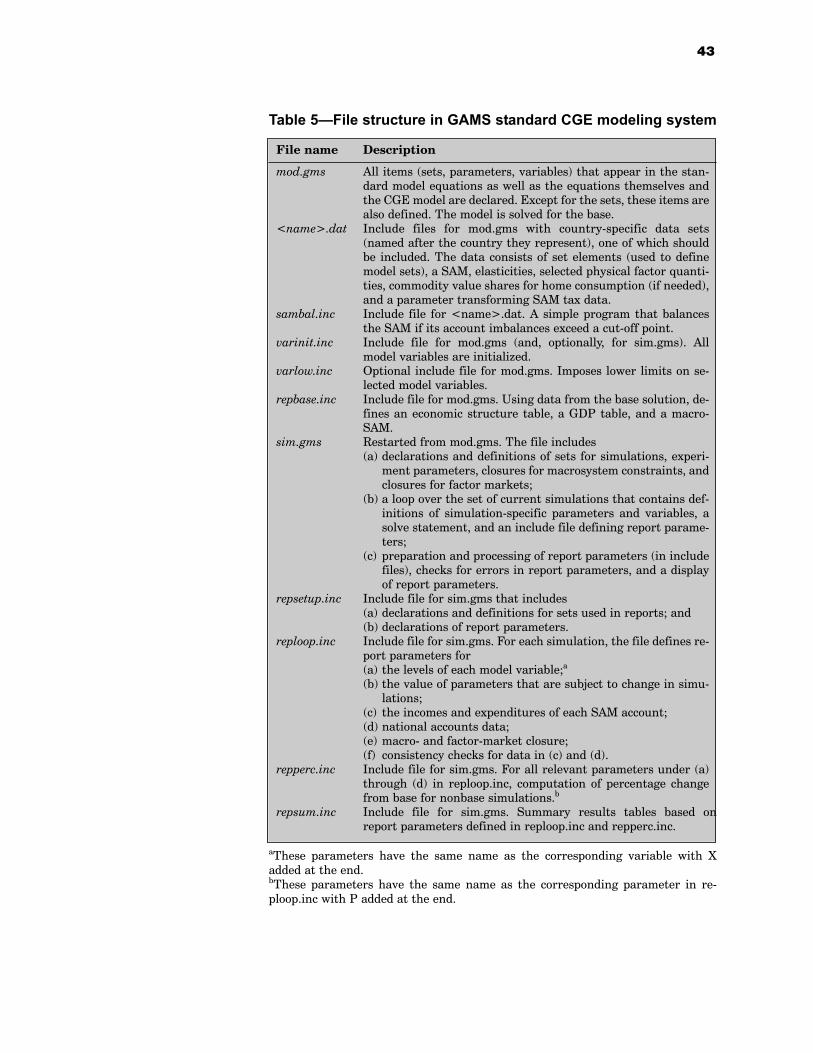
43
Table 5File structure in GAMS standard CGE modeling system
File name Description
mod.gms All items (sets, parameters, variables) that appear in the stan-dard model equations as well as the equations themselves andthe CGE model are declared. Except for the sets, these items arealso defined. The model is solved for the base.
<name>.dat Include files for mod.gms with country-specific data sets(named after the country they represent), one of which shouldbe included. The data consists of set elements (used to definemodel sets), a SAM, elasticities, selected physical factor quanti-ties, commodity value shares for home consumption (if needed),and a parameter transforming SAM tax data.
sambal.inc Include file for <name>.dat. A simple program that balancesthe SAM if its account imbalances exceed a cut-off point.
varinit.inc Include file for mod.gms (and, optionally, for sim.gms). Allmodel variables are initialized.
varlow.inc Optional include file for mod.gms. Imposes lower limits on se-lected model variables.
repbase.inc Include file for mod.gms. Using data from the base solution, de-fines an economic structure table, a GDP table, and a macro-SAM.
sim.gms Restarted from mod.gms. The file includes(a) declarations and definitions of sets for simulations, experi-
ment parameters, closures for macrosystem constraints, andclosures for factor markets;
(b) a loop over the set of current simulations that contains def-initions of simulation-specific parameters and variables, asolve statement, and an include file defining report parame-ters;
(c) preparation and processing of report parameters (in includefiles), checks for errors in report parameters, and a displayof report parameters.
repsetup.inc Include file for sim.gms that includes (a) declarations and definitions for sets used in reports; and (b) declarations of report parameters.
reploop.inc Include file for sim.gms. For each simulation, the file defines re-port parameters for(a) the levels of each model variable;a
(b) the value of parameters that are subject to change in simu-lations;
(c) the incomes and expenditures of each SAM account;(d) national accounts data;(e) macro- and factor-market closure;(f) consistency checks for data in (c) and (d).
repperc.inc Include file for sim.gms. For all relevant parameters under (a)through (d) in reploop.inc, computation of percentage changefrom base for nonbase simulations.b
repsum.inc Include file for sim.gms. Summary results tables based on report parameters defined in reploop.inc and repperc.inc.
aThese parameters have the same name as the corresponding variable with Xadded at the end. bThese parameters have the same name as the corresponding parameter in re-ploop.inc with P added at the end.
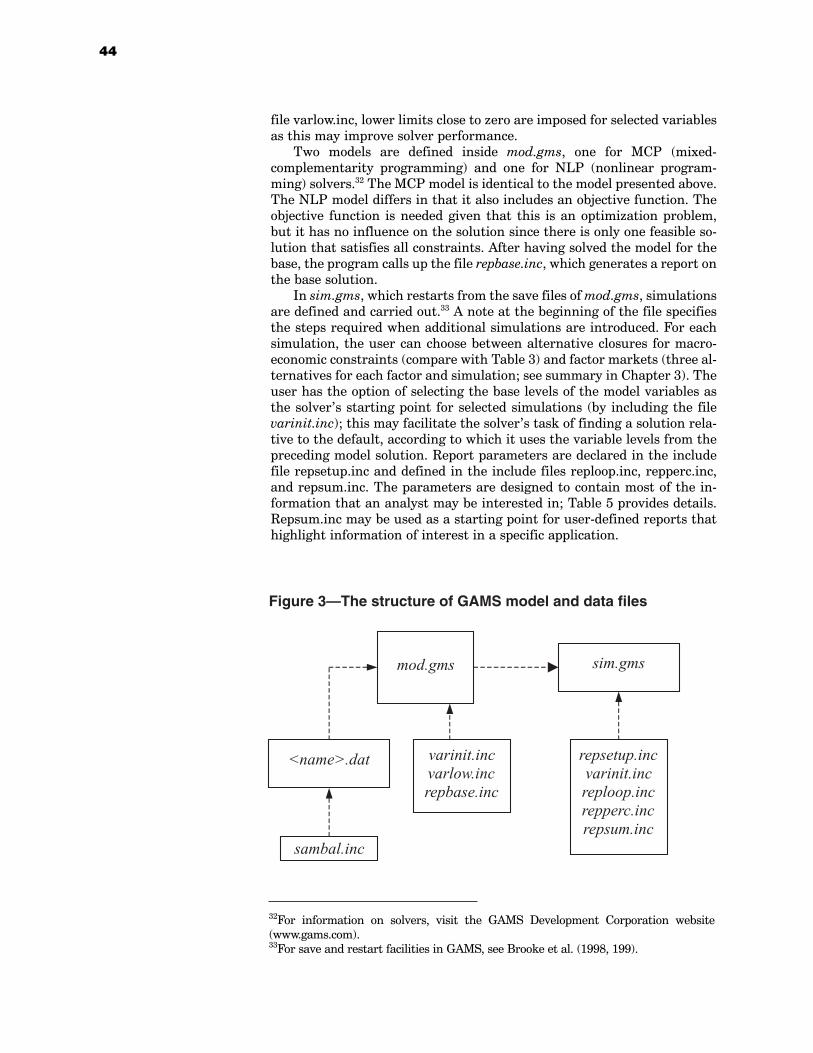
file varlow.inc, lower limits close to zero are imposed for selected variablesas this may improve solver performance.
Two models are defined inside mod.gms, one for MCP (mixed-complementarity programming) and one for NLP (nonlinear program-ming) solvers.32 The MCP model is identical to the model presented above.The NLP model differs in that it also includes an objective function. Theobjective function is needed given that this is an optimization problem,but it has no influence on the solution since there is only one feasible so-lution that satisfies all constraints. After having solved the model for thebase, the program calls up the file repbase.inc, which generates a report onthe base solution.
In sim.gms, which restarts from the save files of mod.gms, simulationsare defined and carried out.33 A note at the beginning of the file specifiesthe steps required when additional simulations are introduced. For eachsimulation, the user can choose between alternative closures for macro-economic constraints (compare with Table 3) and factor markets (three al-ternatives for each factor and simulation; see summary in Chapter 3). Theuser has the option of selecting the base levels of the model variables asthe solvers starting point for selected simulations (by including the filevarinit.inc); this may facilitate the solvers task of finding a solution rela-tive to the default, according to which it uses the variable levels from thepreceding model solution. Report parameters are declared in the includefile repsetup.inc and defined in the include files reploop.inc, repperc.inc,and repsum.inc. The parameters are designed to contain most of the in-formation that an analyst may be interested in; Table 5 provides details.Repsum.inc may be used as a starting point for user-defined reports thathighlight information of interest in a specific application.
44
32For information on solvers, visit the GAMS Development Corporation website(www.gams.com).33For save and restart facilities in GAMS, see Brooke et al. (1998, 199).
mod.gms sim.gms
repsetup.inc
varinit.inc
reploop.inc
repperc.inc
repsum.inc
varinit.inc
varlow.inc
repbase.inc
sambal.inc
<name>.dat
Figure 3—The structure of GAMS model and data files
The modeling system presented can be used in a variety of ways. Thefirst and most straightforward approach is to carry out simulations withone of the existing data sets without making any changes in the modelingstructure. Here the user is required only to define new simulations. Thefile sim.gms includes a note that summarizes the core steps to take whencarrying out additional simulations.
In a second approach, users may wish to take the additional step of ap-plying the model to their own data set. If so, it is preferable to structurethe data set in the same way as the sample data files. The most critical ad-ditional step is to generate a properly formatted SAM. If an available SAMhas a different format (for example, exports from activity accounts insteadof commodity accounts or a different treatment of taxes), we strongly rec-ommend that the user reformat the SAM (a task that can be done insidethe GAMS include file). The alternative of adjusting the model code to adifferently formatted SAM is likely to be more time-consuming and error-prone. Once the model properly calibrates to the new data set, the usercan proceed with simulations.
The third approach is also the most involved. Here, in combinationwith 1 and 2, more advanced users may wish to change the model, a stepthat involves changing the files mod.gms and, quite likely, <name>.dat,as existing model elements (sets, parameters, variables, and equations)are modified or new ones are declared and defined. If the user is also ap-plying the model to a new data set (as in the second approach above), it isprobably easier to divide the process into two steps, first generating a dataset to which the original model calibrates and second modifying the model.Changes in the model structure will also require the user to modify and/oradd to the report system, for example, adding new parameters to accountfor new model variables and modifying the parameters that define the in-comes and expenditures of SAM accounts.34
After having read this manual, we recommend that users familiarizethemselves with the contents of the different files. For users who limitthemselves to the first approach, the most important task is to become fa-miliar with the file sim.gms and its include files. For users who also addtheir own database, as in the second approach described above, it is alsocrucial to be aware of the detailed structure of the standard SAM (de-scribed in Chapter 2 and exemplified in the country data files) and how itmay differ from the original format of any new SAM that the user wantsto apply. A thorough study of the modeling system is required for userswho, in addition, wish to modify the model, using it as a tool to developfurther in different directions.
45
34The modeling system includes consistency checks on the report parameters that willgenerate error messages if, for example, the reports show imbalances between the in-come and spending of SAM accounts.
MATHEMATICAL SUMMARYSTATEMENT FOR THE STANDARDCGE MODEL
α ∈A activities
α ∈ACES(⊂ A) activities with a CES function at the top of the technology nest
α ∈ALEO(⊂ A) activities with a Leontief function at the top of thetechnology nest
c ∈C commodities
c ∈CD(⊂ C) commodities with domestic sales of domestic output
c ∈CDN(⊂ C) commodities not in CD
c ∈CE(⊂ C) exported commodities
c ∈CEN(⊂ C) commodities not in CE
c ∈CM(⊂ C) imported commodities
c ∈CMN(⊂ C) commodities not in CM
c ∈CT(⊂ C) transactions service commodities
c ∈CX(⊂ C) commodities with domestic production
f ∈F factors
i ∈INS institutions (domestic and rest of the world)
i ∈INSD(⊂ INS) domestic institutions
i ∈INSDNG
(⊂ INSD) domestic nongovernment institutions
h ∈H(⊂ INSDNG) households
cwtsc weight of commodity c in the CPIdwtsc weight of commodity c in the producer price indexicac a quantity of c as intermediate input per unit of
activity aicdc c quantity of commodity c as trade input per unit of c
produced and sold domesticallyicec c quantity of commodity c as trade input per exported
unit of cicmc c quantity of commodity c as trade input per imported
unit of c intaa quantity of aggregate intermediate input per activity
unit
SETS
PARAMETERSLatin Letters
APPENDIX A:
46
ivaa quantity of value-added per activity unitmpsi base savings rate for domestic institution imps01c 0-1 parameter with 1 for institutions with potentially
flexed direct tax ratespwec export price (foreign currency)pwmc import price (foreign currency)qdstc quantity of stock changeqgc base-year quantity of government demandqinvc base-year quantity of private investment demandshif i f share for domestic institution i in income of factor fshii i i share of net income of i to i (i ∈INSDNG;
i ∈INSDNG)
tαα tax rate for activity a
tec export tax ratetff direct tax rate for factor ftinsi exogenous direct tax rate for domestic institution itins01i 0-1 parameter with 1 for institutions with potentially
flexed direct tax ratestmc import tariff ratetqc rate of sales taxtrnsfri f transfer from factor f to institution itvaa rate of value-added tax for activity a
α aa efficiency parameter in the CES activity function
α vaa efficiency parameter in the CES value-added function
α aca shift parameter for domestic commodity aggregation
functionα q
c Armington function shift parameter
α tc CET function shift parameter
β ha c h marginal share of consumption spending on home
commodity c from activity a for household hβ m
c h marginal share of consumption spending on marketedcommodity c for household h
δ aa CES activity function share parameter
δ aca c share parameter for domestic commodity aggregation
functionδ q
c Armington function share parameter
δ tc CET function share parameter
δ vaf a CES value-added function share parameter for factor f
in activity aγ m
c h subsistence consumption of marketed commodity c forhousehold h
γ ha c h subsistence consumption of home commodity c from
activity a for household h
47
Greek Letters
48
θ a c yield of output c per unit of activity a
ρ aa CES production function exponent
ρ vaa CES value-added function exponent
ρ acc domestic commodity aggregation function exponent
ρ qc Armington function exponent
ρ tc CET function exponent
CPI
consumer price index DTINS
change in domestic institution tax share (= 0 forbase; exogenous variable)
FSAV
foreign savings (FCU)
GADJ
government consumption adjustment factor
IADJ
investment adjustment factor
MPSADJ
savings rate scaling factor (= 0 for base)
QFS f quantity supplied of factorTINSADJ
direct tax scaling factor (= 0 for base; exogenous vari-able)
WFDIST
f a wage distortion factor for factor f in activity a
DMPS change in domestic institution savings rates (= 0 forbase; exogenous variable)
DPI producer price index for domestically marketed outputEG government expendituresEHh consumption spending for householdEXR exchange rate (LCU per unit of FCU)GOVSHR government consumption share in nominal absorptionGSAV government savingsINVSHR investment share in nominal absorptionMPSi marginal propensity to save for domestic non-
government institution (exogenous variable)PAa activity price (unit gross revenue)PDDc demand price for commodity produced and sold
domesticallyPDSc supply price for commodity produced and sold
domesticallyPEc export price (domestic currency)PINTAa aggregate intermediate input price for activity aPMc import price (domestic currency)PQc composite commodity pricePVAa value-added price (factor income per unit of activity)PXc aggregate producer price for commodityPXACa c producer price of commodity c for activity aQAa quantity (level) of activityQDc quantity sold domestically of domestic output
EXOGENOUSVARIABLES
ENDOGENOUSVARIABLES
49
QEc quantity of exportsQFf a quantity demanded of factor f from activity aQGc government consumption demand for commodityQHc h quantity consumed of commodity c by household hQHAa c h quantity of household home consumption of
commodity c from activity a for household hQINTAa quantity of aggregate intermediate inputQINTc a quantity of commodity c as intermediate input to
activity aQINVc quantity of investment demand for commodityQMc quantity of imports of commodityQQc quantity of goods supplied to domestic market
(composite supply)QTc quantity of commodity demanded as trade inputQVAa quantity of (aggregate) value-addedQXc aggregated marketed quantity of domestic output of
commodityQXACa c quantity of marketed output of commodity c from
activity aTABS total nominal absorptionTINSi direct tax rate for institution i (i ∈ INSDNG)
TRIIi i transfers from institution i to i (both in the set INSDNG)
WFf average price of factor fYFf income of factor fYG government revenueYIi income of domestic nongovernment institutionYIFi f income to domestic institution i from factor f
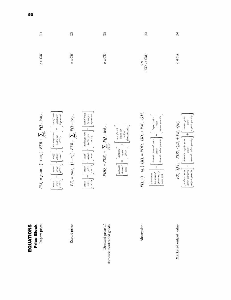
50
EQ
UATIO
NS
Pri
ce B
lock
Impo
rt p
rice
c ∈
CM
(1)
Exp
ort
pric
ec
∈C
E(2
)
Dem
and
pric
e of
c
∈C
D(3
)do
mes
tic
nont
rade
d go
ods
Abs
orpt
ion
(CD
c ∈ ∪ C
M)
(4)
Mar
kete
d ou
tput
val
uec
∈C
X(5
)
PMpw
mtm
EXR
PQic
mc
cc
cc
cc
CT
impo
rtpr
ice
LCU
=⋅
+(
)⋅+
⋅
∈∑1
''
'
()
=
⋅
⋅im
port
pric
eFC
U
tari
ffad
just
men
t(
)-
eexch
ange
rate
LCU
per
FCU
()
+co
st o
f tra
dein
puts
per
imppo
rt u
nit
PEpw
ete
EXR
PQic
ec
cc
cc
cc
CT
pric
eLC
U
=⋅
−(
)⋅−
⋅
∈∑1
''
'
()
expo
rt
=
⋅
⋅ex
port
-pr
ice
FCU
tari
ffad
just
men
t(
)
eexch
ange
rate
LCU
per
FCU
()
−co
st o
f tra
dein
puts
per
exppo
rt u
nit
PDD
PDS
PQic
dc
cc
cc
cC
T
dom
estic
dem
and
pric
e
=+
⋅
=
∈∑'
''
domm
estic
supp
lypr
ice
cost
of t
rade
inpu
ts p
erun
it of
+ddo
mes
tic sa
les
PQtq
PDD
QD
PMQ
Mc
cc
cc
cc
abso
rptio
nat
dem
and
pric
esn
⋅−
()⋅
=⋅
+⋅
1
(eet
ofsa
lest
ax
dom
estic
dem
and
pric
etim
esdo
mes
ticsa
l)
=ees
quan
tity
impo
rtpr
ice
times
impo
rtqu
antit
y
+
PXQ
XPD
SQ
DPE
QE
cc
cc
cc
prod
ucer
pric
etim
esm
arke
ted
outp
utqu
⋅=
⋅+
⋅
aantit
y
dom
estic
pric
etim
esdo
mes
ticsa
les
quan
t
=su
pply
iity
expo
rtpr
ice
times
expo
rtqu
antit
y
+
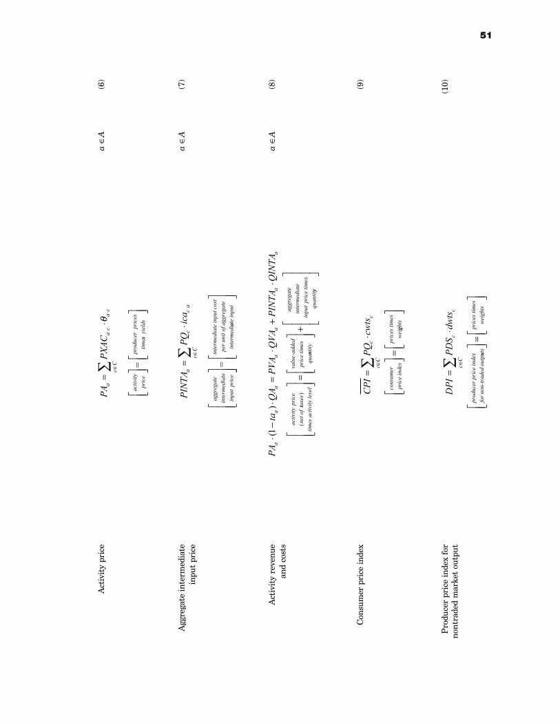
51
Act
ivit
y pr
ice
a ∈
A(6
)
Agg
rega
te in
term
edia
tea
∈A
(7)
inpu
t pr
ice
Act
ivit
y re
venu
e a
∈A
(8)
and
cost
s
Con
sum
er p
rice
inde
x(9
)
Pro
duce
r pr
ice
inde
x fo
r (1
0)no
ntra
ded
mar
ket
outp
ut
PAPX
ACa
ac
ac
cC
=⋅
∈∑
activ
itypr
ice
prod
ucer
pric
estim
e=
θ
ssyi
elds
PIN
TAPQ
ica
ac
ca
cC
=⋅
∈∑
aggr
egat
e in
term
edia
tein
put
pric
e =
inte
rmed
iate
inpu
t cos
tpe
r uni
t of a
ggre
gate
inte
rmed
iaate
inpu
t
PAta
QA
PVA
QVA
PIN
TAQ
INTA
aa
aa
aa
a
activ
itypr
ice
neto
f
⋅−
⋅=
⋅+
⋅(
)
(
1
ttaxe
stim
esac
tivity
leve
l
valu
ead
ded
pric
etim
esqu
a)
=- nnt
ity
aggr
egat
em
edia
tein
put
pric
etim
esqu
antit
+in
ter
yy
CPI
PQcw
tsc
cC
c=
⋅
=
∈∑co
nsum
erpr
ice
inde
xpr
ices
tim
esw
eiggh
ts
DPI
PDS
dwts
cc
Cc
=⋅
∈∑pr
oduc
er p
rice
inde
x fo
r non
-trad
ed o
utpuu
tspr
ices
tim
esw
eigh
ts
=
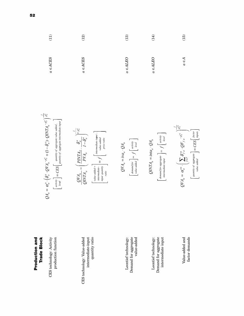
52
Pro
ducti
on a
nd
Trade B
lock
CE
S te
chno
logy
: Act
ivit
ya
∈A
CE
S(1
1)
prod
ucti
on f
unct
ion
CE
S te
chno
logy
: Val
ue-a
dded
a ∈
AC
ES
(12)
inte
rmed
iate
-inp
ut
quan
tity
rat
io
Leo
ntie
f te
chno
logy
: a
∈A
LE
O(1
3)D
eman
d fo
r ag
greg
ate
valu
e-ad
ded
Leo
ntie
f te
chno
logy
:a
∈A
LE
O(1
4)D
eman
d fo
r ag
greg
ate
inte
rmed
iate
inpu
t
Valu
e-ad
ded
and
a ∈
A(1
5)fa
ctor
dem
ands
QVA
QIN
TA =
PIN
TAPV
A1
a
a
a
a
aa
aa
11+
valu
ead
ded
aa
⋅−
δδ
ρ
-−−
=in
term
edia
tein
put
quan
tity
ratio
inte
rmed
iate
inf
--
pput
valu
ead
ded
pric
era
tio
:-
QVA
iva
QA
aa
a=
⋅
de
man
d fo
r va
lue
adde
dac
tivity
le
vel
=f
QIN
TAin
aQ
Aa
aa
=⋅
t
dem
and
for a
ggre
gate
in
term
edia
te in
put
=
fac
tivity
le
vel
QVA
Q
Fa
avaf
ava
fa
fF
-1
quan
tity
ofag
g
avaava
=⋅
⋅
−
∈∑α
δρ
ρ
rre
gate
valu
ead
ded
fact
orin
puts
CES
=
QA
Q
VAQ
INTA
aaa
aaa
aaa
-1
activ
ityle
v
aaaa
aa=
⋅⋅
+−
⋅(
)−
−α
δδ
ρρ
ρ(
)1
eelqu
antit
yof
aggr
egat
eval
uead
ded
quan
tity
ofag
gC
ES
=
,
rrega
tein
term
edia
tein
put
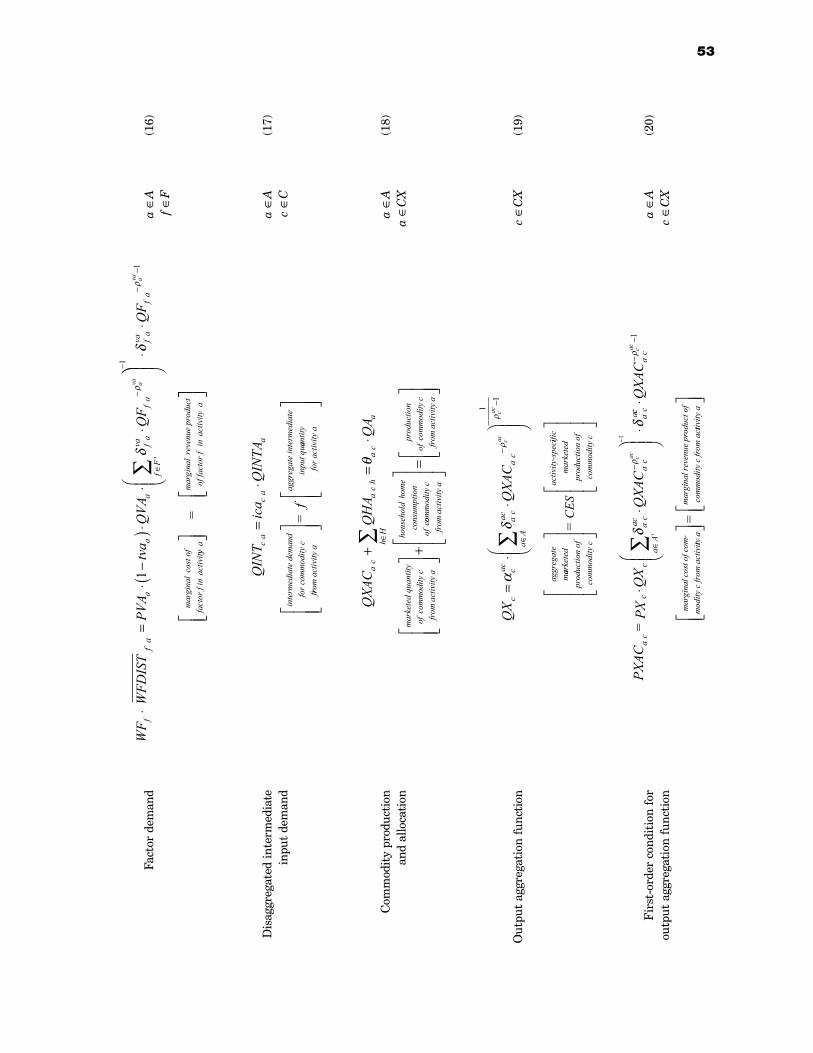
53
Fact
or d
eman
da
∈A
(16)
f ∈
F
Dis
aggr
egat
ed in
term
edia
tea
∈A
(17)
inpu
t de
man
dc
∈C
Com
mod
ity
prod
ucti
on
a ∈
A(1
8)an
d al
loca
tion
a ∈
CX
Out
put
aggr
egat
ion
func
tion
c ∈
CX
(19)
Fir
st-o
rder
con
diti
on f
or
a ∈
A(2
0)ou
tput
agg
rega
tion
fun
ctio
nc
∈C
X
WF
PVA
tva
QVA
QF
fa
aa
fa
vaf
af
Ff
ava⋅
=⋅
−(
)⋅⋅
⋅
−
∈∑ W
FDIS
T a
1δ
ρ
'
⋅
⋅−
−−
1
1δ
ρf
ava
fa
QF
ava
mar
gina
lco
st o
ffa
ctor
f in
activ
ityya
mar
gina
lre
venu
e pr
oduc
tof
fact
or f
inac
tivity
a=
QIN
Tic
aQ
INTA
ca
ca
a
inte
rmed
iate
dem
and
for c
omm
odity
c
f
=⋅
rrom
act
ivity
a
aggr
egat
e in
term
edia
te
inpu
t qu
=f
aan
tity
for a
ctiv
ity a
QXA
CQ
HA
QA
ac
ac
hh
Ha
ca
mar
kete
d qu
antit
yof
com
mod
ity
+=
⋅∈∑
θ
c fr
om a
ctiv
ity a
hous
ehol
dho
me
cons
umpt
ion
of c
+
oomm
odity
c fr
om a
ctiv
ity a
prod
uctio
nof
com
mod
ity
= c
from
act
ivity
a
QX
QXA
Cc
caca
cac
ac
aA
caccac
=⋅
⋅
−
∈
−−
∑α
δρ
ρ
aggr
egat
em
11
aarke
ted
prod
uctio
n of
com
mod
ity c
activ
ity-s
pec
=C
ES
iific
mar
kete
dpr
oduc
tion
ofco
mm
odity
c
PXAC
= P
XQ
XQ
XAC
a
cc
ca
Aa
cac
ac
ac
acac
⋅⋅
⋅∈
−∑
−
'δδ
ρ1
cca
cQ
XAC
cac⋅
−−
mar
gina
l cos
t of c
om-
mod
ity c
from
act
ivi
ρ1
tty a
mar
gina
l rev
enue
pro
duct
of
com
mod
ity c
from
ac
=
ttiv
ity a
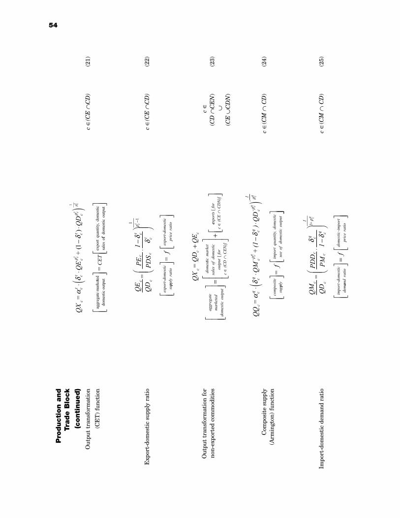
54
Pro
ducti
on a
nd
Trade B
lock
(conti
nued)
Out
put
tran
sfor
mat
ion
c
∈(C
E ∩
CD
)(2
1)
(CE
T)
func
tion
Exp
ort-
dom
esti
c su
pply
rat
ioc
∈(C
E ∩
CD
)(2
2)
Out
put
tran
sfor
mat
ion
for
c ∈
non-
expo
rted
com
mod
itie
s (C
D ∩
CE
N)
(23)
∪(C
E ∪
CD
N)
Com
posi
te s
uppl
y
c ∈
(CM
∩ C
D)
(24)
(Arm
ingt
on)
func
tion
Impo
rt-d
omes
tic
dem
and
rati
o c
∈(C
M ∩
CD
) (2
5)
cct
ctc
ctc
QX
=
QE
+
QD
ctct
ctα
δδ
ρρ
ρ⋅
⋅−
⋅(
)(1
1
)
aggr
egat
e m
arke
tted
dom
estic
out
put
expo
rtqu
antit
y,do
mes
ticsa
les
o=
CET
ffdo
mes
ticou
tput
c c
c c
ct
ct
QE
QD
=
PE PDS
1
ct
⋅−
−δ
δρ
11
expo
rt-d
omes
ticsu
ppply
ratio
expo
rt-d
omes
ticpr
ice
ratio
=f
cc
c
aggr
egat
em
arke
ted
dom
estic
outp
ut
dom
es
QX
= Q
DQ
E+
=ttic
mar
ket
sale
sof
dom
estic
outp
utfo
r
c
(CD
CEN
)][
∈∩
+eex
port
s
c(C
EC
DN
)][f
or∈
∩
ccq
cqc-
cqc-
-1
=
QM
+ (1
)Q
Dcq
cqcq
αδ
δρ
ρρ
⋅⋅
−⋅
()
com
posi
tesu
ppply
impo
rtqu
antit
y,do
mes
ticus
eof
dom
estic
outp
ut=
f
QM QD
=PD
DPM
1
c c
c c
cq
cq
11+
impo
rtdo
mes
ticde
m
cq
⋅−
δδ
ρ
- aand
ratio
dom
estic
impo
rtpr
ice
ratio
f
=
-
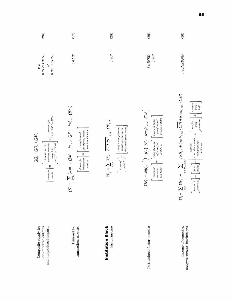
55
Com
posi
te s
uppl
y fo
r c
∈no
n-im
port
ed o
utpu
ts
(CD
∩ C
MN
)(2
6)
and
nonp
rodu
ced
impo
rts
∪(C
M ∪
CD
N)
Dem
and
for
c
∈C
T(2
7)tr
ansa
ctio
ns s
ervi
ces
Inst
ituti
on B
lock
Fact
or in
com
ef
∈F
(28)
Inst
itut
iona
l fac
tor
inco
mes
i ∈
INS
D(2
9)f
∈F
Inco
me
of d
omes
tic,
i ∈
INS
DN
G(3
0)no
ngov
ernm
ent
inst
itut
ions
cc
c
com
posi
tedo
mes
ticus
eof
mar
kete
d
= Q
D
QM
+
=
supp
ly dd
omes
tic
c
CM
N)]
cou
tput
for
CD
impo
rts
for
C[
(
[(
∈∩
∈
+MM
∩
C
DN
)]
cc
cc
cc
cc
cc
cC
QT
=ic
mQ
Mic
eQ
Eic
dQ
D
dem
and'
''
''
''
'⋅
+⋅
+⋅
()
∈∑ fo
rtr
ansa
ctio
nsse
rvic
es
sum
of d
eman
dsfo
r im
port
=
ss,
expo
rts,
and
dom
estic
sale
s
YF =
WF
Q
Ff
fa
Af
af
∈∑⋅
⋅
WFD
IST
=
a
inco
me
of
fact
or f
sum
of a
ctiv
ity p
aym
ents
(act
ivity
-spe
cific
wag
es
times
em
ployy
men
t lev
els)
YIF
=sh
iftf
YFtr
nsfr
EXR
ifif
ff
row
f
inco
me
of
i
⋅− (
)⋅−
⋅
1
nnstit
utio
n i
from
fact
or f
shar
e of
inco
me
of fa
ct=
oor
f to
inst
itutio
n i
inco
me
of f
acto
r f(n
et o
f t
⋅aax
and
tr
ansf
er to
RoW
)
YI =
YI
FTR
IItr
nsfr
CPI
trns
fri
ifii
igov
iIN
SDN
Gir
++
⋅+
∈∑
''
'oow
fF
EXR
⋅
∈∑ inco
me
of
inst
itutio
n i
fact
orin
com
e=
+
tran
sfer
sfr
omot
her d
omes
ticno
n-go
vern
men
tin
stitu
tions
+
+tr
ansf
ers
from
gove
rnm
ent
tran
sfer
s fr
om
RoWW
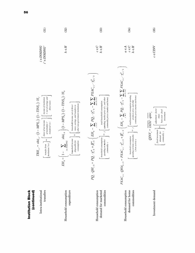
56
Inst
ituti
on B
lock
(conti
nued)
Intr
a-in
stit
utio
nal
i ∈
INS
DN
Gtr
ansf
ers
i ∈
INS
DN
G
(31)
Hou
seho
ld c
onsu
mpt
ion
h
∈H
(32)
expe
ndit
ure
Hou
seho
ld c
onsu
mpt
ion
c ∈
Cde
man
d fo
r m
arke
ted
h ∈
H(3
3)co
mm
odit
ies
Hou
seho
ld c
onsu
mpt
ion
a ∈
Ade
man
d fo
r ho
me
c ∈
C(3
4)co
mm
odit
ies
h ∈
H
Inve
stm
ent
dem
and
c ∈
CIN
V(3
5)
TRII
= sh
iiM
PSTI
NS
YIii
iii
ii
tran
sfer
from'
''
''
⋅−
()⋅
−(
)⋅1
1
iinst
itutio
n i'
to i
shar
e of
net
inco
me
of in
stitu
t=
iion
i'tr
ansf
ered
to i
inco
me
of in
stitu
tion
i', n
et
⋅ o
f sav
ings
and
dir
ect t
axes
EH =
sh
iiM
PSTI
NS
YIh
ihi
INSD
NG
hh
h1
11
−
⋅−
()⋅
−(
)⋅∈∑
houus
ehol
d in
com
e di
spos
able
for
cons
umpt
ion
hous
eho
=
lld in
com
e, n
et o
f dir
ect
taxe
s, sa
ving
s, an
d tr
ansf
ers t
o ot
her n
on-g
over
nmen
t ins
titut
ions
PQQ
H =
PQEH
PQPX
ACc
ch
cc
hmc
hmh
cc
hm
cC
ac
⋅⋅
+⋅
−⋅
−⋅
∈∑
γβ
γγ
''
''
aac
hh
cC
aA
hous
ehol
d co
nsum
ptio
nsp
endi
ng o
n
''∈
∈∑
∑
mmar
ket
com
mod
ityc
fto
tal h
ouse
hold
con
sum
ptio
n sp
=
een
ding
, mar
ket p
rice
of c
, and
oth
er
com
mod
ity p
rice
s (m
arrke
t and
hom
e)
QIN
V =
IAD
Jqi
nvc
c⋅
fixed
inve
stm
ent
dem
and
for
com
mod
ityc
=
adju
stm
ent
fact
ortim
esba
se-y
ear
inve
stm
ent fix
ed
PXAC
QH
A=
PXAC
EHPQ
ac
ac
ha
ca
ch
ha
ch
hh
cc
hm
c
⋅⋅
+⋅
−⋅
γβ
γ'
''∈∈
∈∈
∑∑
∑−
⋅
C
ac
ac
hh
cC
aA
PXAC
hous
ehol
d co
nsum
ptio
n
''
'γ
sspen
ding
on
hom
e co
mm
odity
c fr
om a
ctiv
ity a
fto
ta=
ll hou
seho
ld c
onsu
mpt
ion
spen
ding
, pr
oduc
er p
rice
, and
oth
eer
com
mod
ity p
rice
s (m
arke
t and
hom
e)
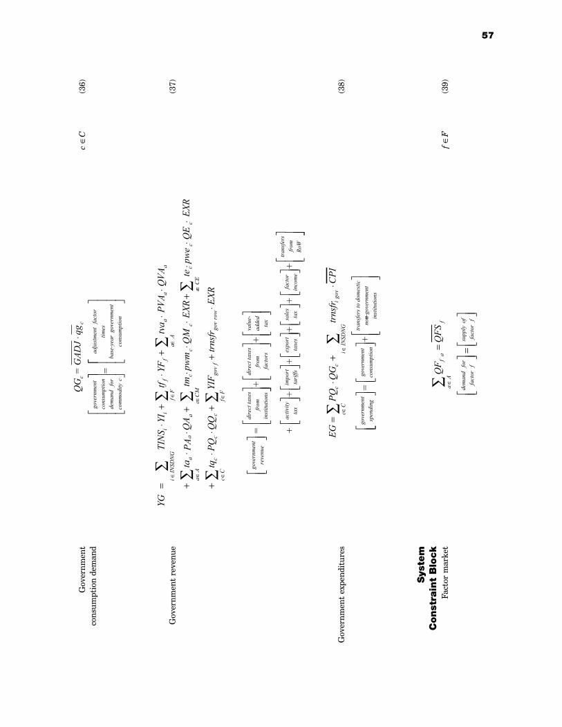
57
Gov
ernm
ent
c ∈
C(3
6)co
nsum
ptio
n de
man
d
Gov
ernm
ent
reve
nue
(37)
Gov
ernm
ent
expe
ndit
ures
(38)
Sys
tem
C
onst
rain
t B
lock
Fact
or m
arke
tf
∈F
(39)
QG
=G
ADJ
qgc
c⋅
gove
rnm
ent
cons
umpt
ion
dem
and
for
com
mod
ityc =
ad
just
men
tfa
ctor
times
base
-yea
rgo
vern
men
tco
nsum
ptio
n
gove
rnm
ent
reve
nue
dire
ct ta
xes
from
inst
itutio
ns=
+
+di
rect
taxe
sfr
om
fact
ors
valu
e-ad
ded
tax
++
+ac
tivity
tax
impo
rtta
riffs
expo
rtta
xes
+
++
sale
sta
xfa
ctor
inco
me
tran
sfer
sfr
omRo
W
ii
ff
aa
ai
INSD
NG
fF
aA
aa
cc
ac
cc
ca
Ac
CM
cC
E
cc
cgo
v f
gov
row
cC
fF
YGTI
NS
YItf
YFtv
aPV
AQ
VA
tatm
EXR
teEX
RQ
Apw
mQ
Mpw
eQ
EPA
tqPQ
YIF
trns
frEX
R
∈∈
∈
∈∈
∈
∈∈
=⋅
+⋅
+⋅
⋅
+⋅
⋅+
⋅⋅
+⋅
⋅⋅
⋅
+⋅
⋅+
+⋅
∑∑
∑
∑∑
∑
∑∑
EGPQ
QG
trns
frC
PIc
cig
ovi
INSD
NG
cC
=⋅
+⋅
∈∈
∑∑
gove
rnm
ent
spen
ding
=+
gove
rnm
ent
cons
umpt
ion
tran
sfer
s to
dom
estic
nonn-
gove
rnm
ent
inst
itutio
ns
QF
QFS
fa
fa
A
dem
and
for
fact
orf
offa
ctor
f
supp
ly
=
=
∈∑
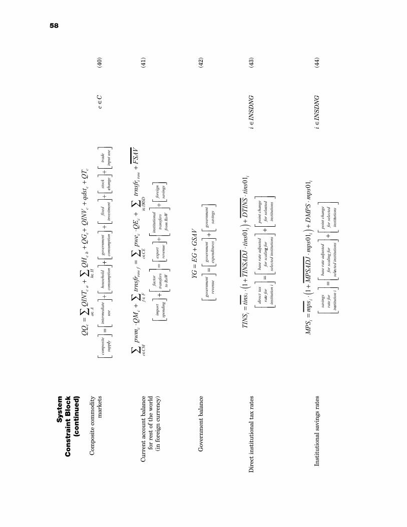
Sys
tem
C
onst
rain
t B
lock
(conti
nued)
Com
posi
te c
omm
odit
ym
arke
tsc
∈C
(40)
Cur
rent
acc
ount
bal
ance
(4
1)fo
r re
st o
f th
e w
orld
(i
n fo
reig
n cu
rren
cy)
Gov
ernm
ent
bala
nce
(42)
Dir
ect
inst
itut
iona
l tax
rat
esi
∈IN
SD
NG
(43)
Inst
itut
iona
l sav
ings
rat
esi
∈IN
SD
NG
(44)
58
QIN
TQ
HQ
GQ
INV
qdst
QT
cc
aa
Ac
hh
Hc
cc
c
com
posi
te
=+
++
++
∈∈
∑∑
supp
llyin
term
edia
teus
eho
useh
old
cons
umpt
ion
+
=
++ +
+go
vern
men
tco
nsum
ptio
nfix
edin
vest
men
tst
ock
cchan
getr
ade
inpu
t use
+
pwm
QM
trns
frpw
eQ
Etr
nsfr
cc
CM
cro
wf
fF
cc
CE
cir
owi
I⋅
+=
⋅+
∈∈
∈∈
∑∑
∑
NN
SDFS
AV∑
+
+
im
port
spen
ding
fact
or
tran
sfer
s to
RoW
=
+ex
port
re
venu
e
inst
itutio
nal
tran
sfer
sfr
om R
oW
+
fore
ign
savi
ngs
TIN
Stin
sTI
NSA
DJ
tins
DTI
NS
tins
ii
ii
dire
ct
=⋅
+⋅
()+
⋅1
0101
tax
ratte
inst
itutio
n i
base
rate
adj
uste
dfo
r sca
linfo
r
=gg
for
sele
cted
inst
itutio
ns
poin
t cha
nge
for s
ele
+cct
edin
stitu
tions
MPS
mps
MPS
ADJ
mps
DM
PSm
psi
ii
i
savi
ngs
for
=⋅
+⋅
()+
⋅1
0101
ra
te
in
sstitu
tion
i
base
rate
adj
uste
dfo
r sca
ling
for
sel
=eec
ted
inst
itutio
ns
poin
t cha
nge
for s
elec
ted
inst
i
+ttu
tions
gove
rnm
ent
gove
rnm
ent
gove
rnm
ent
reve
nue
expe
nditu
res
savi
ngs
YGEG
GSA
V=
+
=+
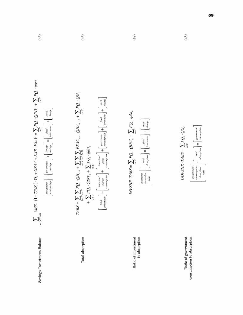
59
Savi
ngs
Inve
stm
ent
Bal
ance
(45)
Tot
al a
bsor
ptio
n(4
6)
Rat
io o
f in
vest
men
t(4
7)to
abs
orpt
ion
Rat
io o
f go
vern
men
t (4
8)co
nsum
ptio
n to
abs
orpt
ion
MPS
TIN
SYI
GSA
VEX
RFS
AVPQ
QIN
VPQ
ii
iIN
SDN
Gi
cc
Cc
⋅−
()⋅
++
⋅=
⋅+
∈∈
∑∑
1cc
cc
Cqd
st⋅
+
∈∑no
n-go
vern
-m
ent s
avin
gsgo
vern
men
tsa
ving
ssfo
reig
nsa
ving
sfix
edin
vest
men
tst
ock
+
=
+cch
ange
TABS
PQQ
HPX
ACQ
HA
PQQ
Gc
cC
hH
ch
ac
ac
hh
Hc
Ca
Ac
=⋅
+⋅
+⋅
∈∈
∈∈
∈∑
∑∑
∑∑
ccc
C
cc
cC
cc
cC
PQQ
INV
PQqd
st∈
∈∈
∑
∑∑
+⋅
+⋅
=
tota
l ab
sorp
tion
hoous
ehol
dm
arke
tco
nsum
ptio
n
hous
ehol
dho
me
cons
umpt
io
+nn
gove
rnm
ent
cons
umpt
ion
fixed
inve
stm
ent
+
+
+
st
ock
chan
ge
INVS
HR
TABS
PQQ
INV
PQqd
stc
cc
Cc
cc
C⋅
=⋅
+⋅
∈∈
∑∑
inve
stm
ent-
abso
rptioo
nra
tio
tota
lab
sorp
tion
fixed
inve
stm
ent
⋅ =
+
stoc
kch
ange
GO
VSH
RTA
BSPQ
QG
cc
Cc
⋅=
⋅∈∑
gove
rnm
ent
cons
umpt
ion-
abso
rptio
nra
tiio
tota
lab
sorp
tion
gove
rnm
ent
cons
umpt
ion
⋅ =
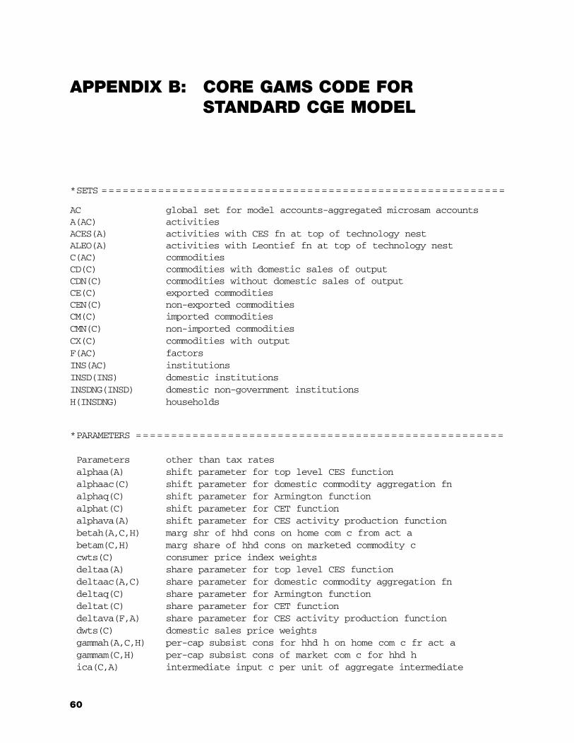
*SETS = = = = = = = = = = = = = = = = = = = = = = = = = = = = = = = = = = = = = = = = = = = = = = = = = = = = = = = = =
AC global set for model accounts-aggregated microsam accounts A(AC) activities ACES(A) activities with CES fn at top of technology nest ALEO(A) activities with Leontief fn at top of technology nestC(AC) commodities CD(C) commodities with domestic sales of output CDN(C) commodities without domestic sales of output CE(C) exported commodities CEN(C) non-exported commodities CM(C) imported commodities CMN(C) non-imported commodities CX(C) commodities with output F(AC) factors INS(AC) institutions INSD(INS) domestic institutions INSDNG(INSD) domestic non-government institutions H(INSDNG) households
*PARAMETERS = = = = = = = = = = = = = = = = = = = = = = = = = = = = = = = = = = = = = = = = = = = = = = = = = = = =
Parameters other than tax rates alphaa(A) shift parameter for top level CES function alphaac(C) shift parameter for domestic commodity aggregation fn alphaq(C) shift parameter for Armington function alphat(C) shift parameter for CET function alphava(A) shift parameter for CES activity production function betah(A,C,H) marg shr of hhd cons on home com c from act a betam(C,H) marg share of hhd cons on marketed commodity ccwts(C) consumer price index weights deltaa(A) share parameter for top level CES function deltaac(A,C) share parameter for domestic commodity aggregation fndeltaq(C) share parameter for Armington function deltat(C) share parameter for CET function deltava(F,A) share parameter for CES activity production function dwts(C) domestic sales price weights gammah(A,C,H) per-cap subsist cons for hhd h on home com c fr act a gammam(C,H) per-cap subsist cons of market com c for hhd h ica(C,A) intermediate input c per unit of aggregate intermediate
APPENDIX B: CORE GAMS CODE FOR STANDARD CGE MODEL
60
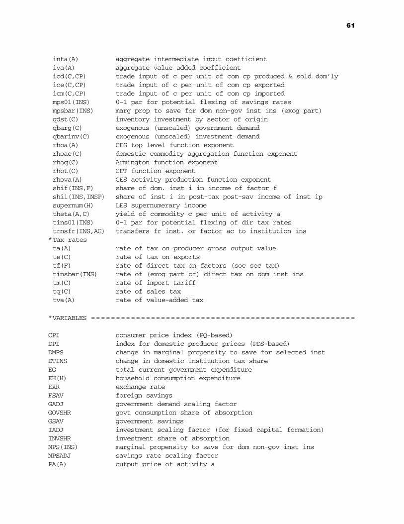
61
inta(A) aggregate intermediate input coefficient iva(A) aggregate value added coefficient icd(C,CP) trade input of c per unit of com cp produced & sold dom’ly ice(C,CP) trade input of c per unit of com cp exported icm(C,CP) trade input of c per unit of com cp imported mps01(INS) 0-1 par for potential flexing of savings rates mpsbar(INS) marg prop to save for dom non-gov inst ins (exog part) qdst(C) inventory investment by sector of origin qbarg(C) exogenous (unscaled) government demand qbarinv(C) exogenous (unscaled) investment demand rhoa(A) CES top level function exponent rhoac(C) domestic commodity aggregation function exponent rhoq(C) Armington function exponent rhot(C) CET function exponent rhova(A) CES activity production function exponent shif(INS,F) share of dom. inst i in income of factor f shii(INS,INSP) share of inst i in post-tax post-sav income of inst ip supernum(H) LES supernumerary income theta(A,C) yield of commodity c per unit of activity a tins01(INS) 0-1 par for potential flexing of dir tax rates trnsfr(INS,AC) transfers fr inst. or factor ac to institution ins
*Tax ratesta(A) rate of tax on producer gross output value te(C) rate of tax on exports tf(F) rate of direct tax on factors (soc sec tax) tinsbar(INS) rate of (exog part of) direct tax on dom inst ins tm(C) rate of import tariff tq(C) rate of sales tax tva(A) rate of value-added tax
*VARIABLES = = = = = = = = = = = = = = = = = = = = = = = = = = = = = = = = = = = = = = = = = = = = = = = = = = = = =
CPI consumer price index (PQ-based) DPI index for domestic producer prices (PDS-based) DMPS change in marginal propensity to save for selected inst DTINS change in domestic institution tax share EG total current government expenditure EH(H) household consumption expenditure EXR exchange rate FSAV foreign savings GADJ government demand scaling factor GOVSHR govt consumption share of absorption GSAV government savings IADJ investment scaling factor (for fixed capital formation) INVSHR investment share of absorption MPS(INS) marginal propensity to save for dom non-gov inst ins MPSADJ savings rate scaling factor PA(A) output price of activity a
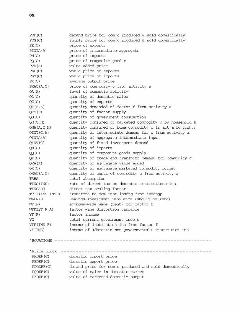
62
PDD(C) demand price for com c produced & sold domestically PDS(C) supply price for com c produced & sold domestically PE(C) price of exports PINTA(A) price of intermediate aggregate PM(C) price of imports PQ(C) price of composite good c PVA(A) value added price PWE(C) world price of exports PWM(C) world price of imports PX(C) average output price PXAC(A,C) price of commodity c from activity a QA(A) level of domestic activity QD(C) quantity of domestic sales QE(C) quantity of exports QF(F,A) quantity demanded of factor f from activity a QFS(F) quantity of factor supply QG(C) quantity of government consumption QH(C,H) quantity consumed of marketed commodity c by household h QHA(A,C,H) quantity consumed of home commodity c fr act a by hhd h QINT(C,A) quantity of intermediate demand for c from activity a QINTA(A) quantity of aggregate intermediate input QINV(C) quantity of fixed investment demand QM(C) quantity of imports QQ(C) quantity of composite goods supply QT(C) quantity of trade and transport demand for commodity c QVA(A) quantity of aggregate value added QX(C) quantity of aggregate marketed commodity output QXAC(A,C) quantity of ouput of commodity c from activity a TABS total absorption TINS(INS) rate of direct tax on domestic institutions ins TINSADJ direct tax scaling factor TRII(INS,INSP) transfers to dom inst insdng from insdngp WALRAS Savings–Investment imbalance (should be zero) WF(F) economy-wide wage (rent) for factor f WFDIST(F,A) factor wage distortion variable YF(F) factor income YG total current government income YIF(INS,F) income of institution ins from factor f YI(INS) income of (domestic non-governmental) institution ins
*EQUATIONS = = = = = = = = = = = = = = = = = = = = = = = = = = = = = = = = = = = = = = = = = = = = = = = = = = = = =
*Price block = = = = = = = = = = = = = = = = = = = = = = = = = = = = = = = = = = = = = = = = = = = = = = = = = = =PMDEF(C) domestic import price PEDEF(C) domestic export price PDDDEF(C) demand price for com c produced and sold domestically PQDEF(C) value of sales in domestic market PXDEF(C) value of marketed domestic output
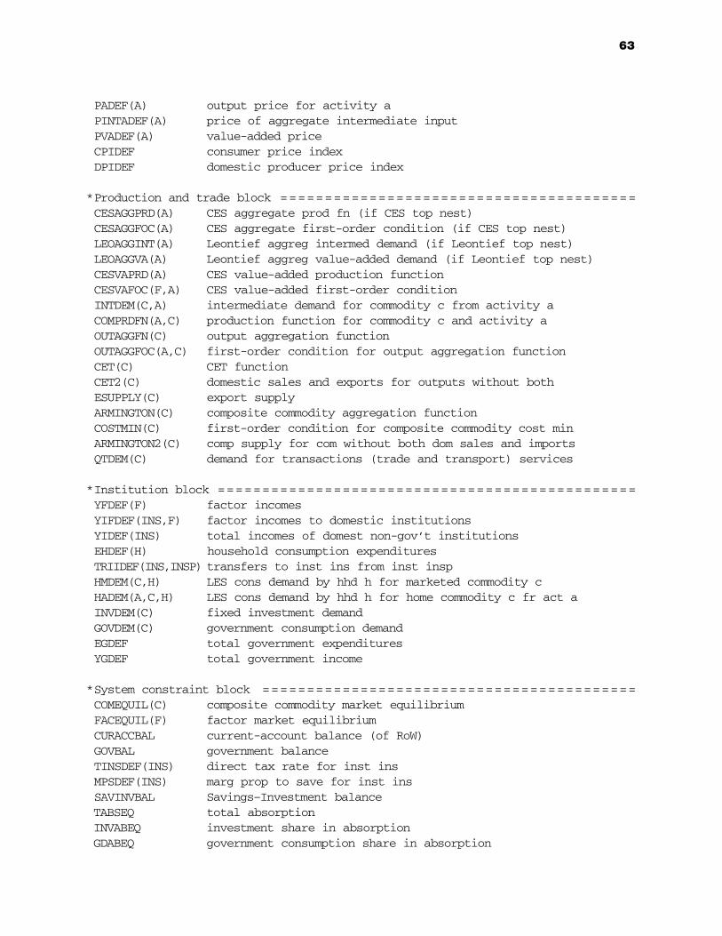
63
PADEF(A) output price for activity a PINTADEF(A) price of aggregate intermediate input PVADEF(A) value-added price CPIDEF consumer price index DPIDEF domestic producer price index
*Production and trade block = = = = = = = = = = = = = = = = = = = = = = = = = = = = = = = = = = = = = = = =CESAGGPRD(A) CES aggregate prod fn (if CES top nest) CESAGGFOC(A) CES aggregate first-order condition (if CES top nest) LEOAGGINT(A) Leontief aggreg intermed demand (if Leontief top nest) LEOAGGVA(A) Leontief aggreg value-added demand (if Leontief top nest) CESVAPRD(A) CES value-added production function CESVAFOC(F,A) CES value-added first-order condition INTDEM(C,A) intermediate demand for commodity c from activity a COMPRDFN(A,C) production function for commodity c and activity a OUTAGGFN(C) output aggregation function OUTAGGFOC(A,C) first-order condition for output aggregation function CET(C) CET function CET2(C) domestic sales and exports for outputs without both ESUPPLY(C) export supply ARMINGTON(C) composite commodity aggregation function COSTMIN(C) first-order condition for composite commodity cost min ARMINGTON2(C) comp supply for com without both dom sales and imports QTDEM(C) demand for transactions (trade and transport) services
*Institution block = = = = = = = = = = = = = = = = = = = = = = = = = = = = = = = = = = = = = = = = = = = = = = =YFDEF(F) factor incomes YIFDEF(INS,F) factor incomes to domestic institutions YIDEF(INS) total incomes of domest non-gov’t institutions EHDEF(H) household consumption expenditures TRIIDEF(INS,INSP) transfers to inst ins from inst insp HMDEM(C,H) LES cons demand by hhd h for marketed commodity c HADEM(A,C,H) LES cons demand by hhd h for home commodity c fr act a INVDEM(C) fixed investment demand GOVDEM(C) government consumption demand EGDEF total government expenditures YGDEF total government income
*System constraint block = = = = = = = = = = = = = = = = = = = = = = = = = = = = = = = = = = = = = = = = = =COMEQUIL(C) composite commodity market equilibrium FACEQUIL(F) factor market equilibrium CURACCBAL current-account balance (of RoW) GOVBAL government balance TINSDEF(INS) direct tax rate for inst ins MPSDEF(INS) marg prop to save for inst ins SAVINVBAL Savings–Investment balance TABSEQ total absorption INVABEQ investment share in absorption GDABEQ government consumption share in absorption
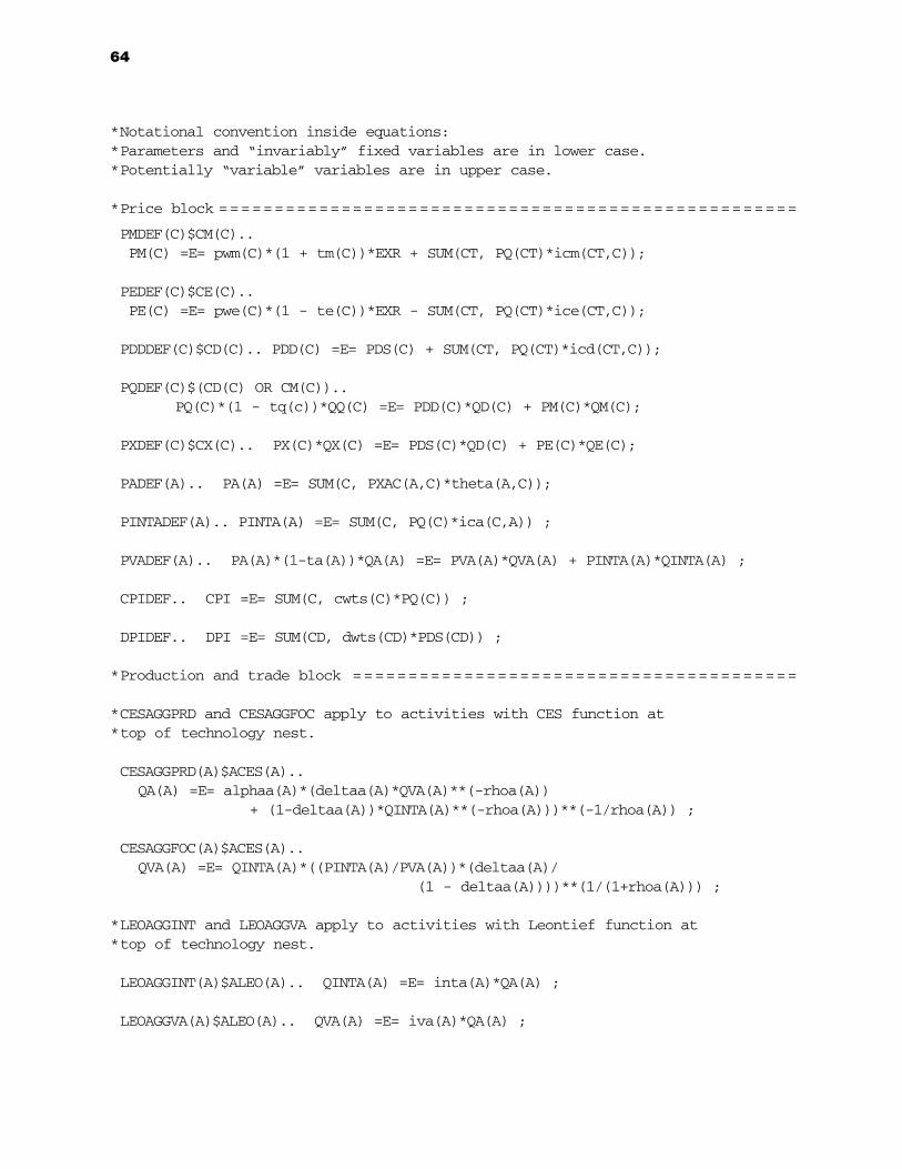
64
*Notational convention inside equations: *Parameters and “invariably” fixed variables are in lower case. *Potentially “variable” variables are in upper case.
*Price block = = = = = = = = = = = = = = = = = = = = = = = = = = = = = = = = = = = = = = = = = = = = = = = = = = = =
PMDEF(C)$CM(C).. PM(C) =E= pwm(C)*(1 + tm(C))*EXR + SUM(CT, PQ(CT)*icm(CT,C));
PEDEF(C)$CE(C).. PE(C) =E= pwe(C)*(1 - te(C))*EXR - SUM(CT, PQ(CT)*ice(CT,C));
PDDDEF(C)$CD(C).. PDD(C) =E= PDS(C) + SUM(CT, PQ(CT)*icd(CT,C));
PQDEF(C)$(CD(C) OR CM(C)).. PQ(C)*(1 - tq(c))*QQ(C) =E= PDD(C)*QD(C) + PM(C)*QM(C);
PXDEF(C)$CX(C).. PX(C)*QX(C) =E= PDS(C)*QD(C) + PE(C)*QE(C);
PADEF(A).. PA(A) =E= SUM(C, PXAC(A,C)*theta(A,C));
PINTADEF(A).. PINTA(A) =E= SUM(C, PQ(C)*ica(C,A)) ;
PVADEF(A).. PA(A)*(1-ta(A))*QA(A) =E= PVA(A)*QVA(A) + PINTA(A)*QINTA(A) ;
CPIDEF.. CPI =E= SUM(C, cwts(C)*PQ(C)) ;
DPIDEF.. DPI =E= SUM(CD, dwts(CD)*PDS(CD)) ;
*Production and trade block = = = = = = = = = = = = = = = = = = = = = = = = = = = = = = = = = = = = = = = =
*CESAGGPRD and CESAGGFOC apply to activities with CES function at *top of technology nest.
CESAGGPRD(A)$ACES(A).. QA(A) =E= alphaa(A)*(deltaa(A)*QVA(A)**(-rhoa(A))
+ (1-deltaa(A))*QINTA(A)**(-rhoa(A)))**(-1/rhoa(A)) ;
CESAGGFOC(A)$ACES(A).. QVA(A) =E= QINTA(A)*((PINTA(A)/PVA(A))*(deltaa(A)/
(1 - deltaa(A))))**(1/(1+rhoa(A))) ;
*LEOAGGINT and LEOAGGVA apply to activities with Leontief function at *top of technology nest.
LEOAGGINT(A)$ALEO(A).. QINTA(A) =E= inta(A)*QA(A) ;
LEOAGGVA(A)$ALEO(A).. QVA(A) =E= iva(A)*QA(A) ;
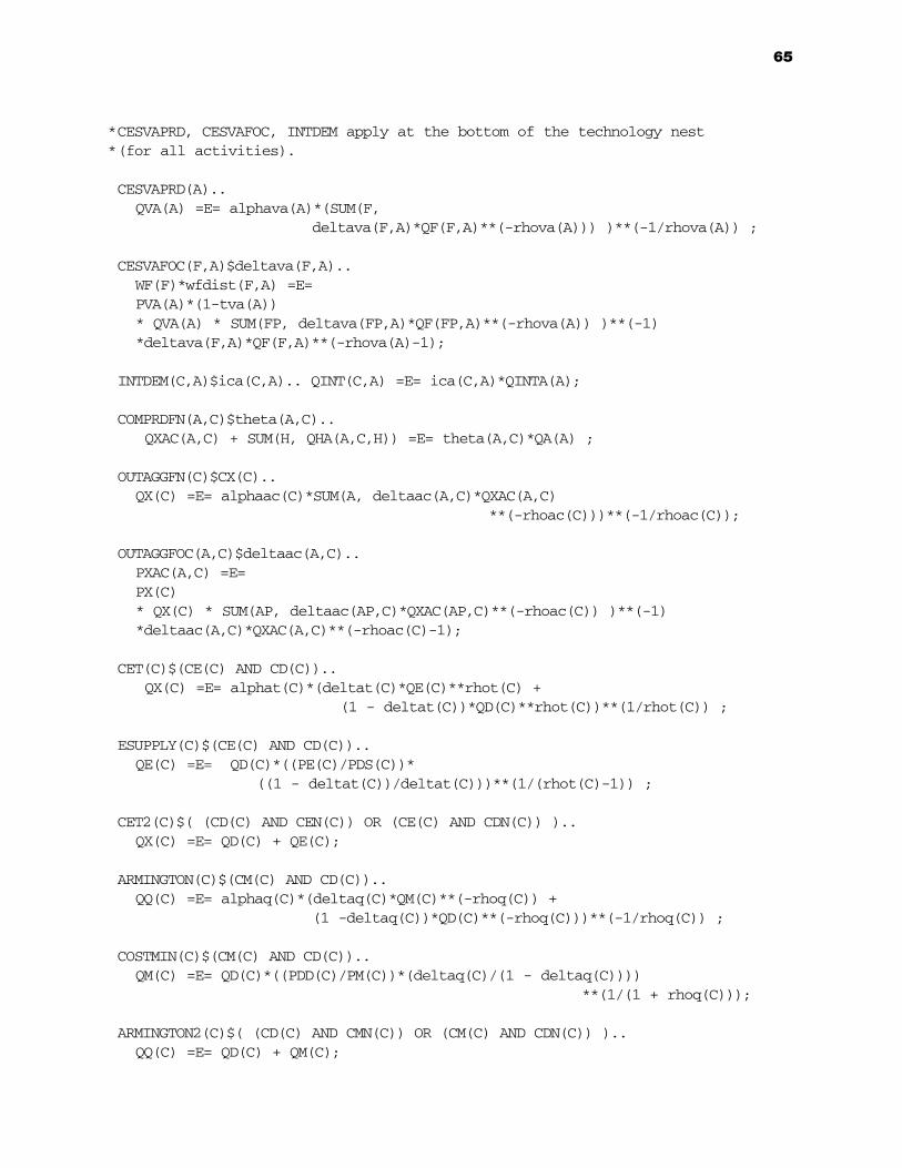
65
*CESVAPRD, CESVAFOC, INTDEM apply at the bottom of the technology nest *(for all activities).
CESVAPRD(A).. QVA(A) =E= alphava(A)*(SUM(F,
deltava(F,A)*QF(F,A)**(-rhova(A))) )**(-1/rhova(A)) ;
CESVAFOC(F,A)$deltava(F,A)..WF(F)*wfdist(F,A) =E=PVA(A)*(1-tva(A))* QVA(A) * SUM(FP, deltava(FP,A)*QF(FP,A)**(-rhova(A)) )**(-1)*deltava(F,A)*QF(F,A)**(-rhova(A)-1);
INTDEM(C,A)$ica(C,A).. QINT(C,A) =E= ica(C,A)*QINTA(A);
COMPRDFN(A,C)$theta(A,C).. QXAC(A,C) + SUM(H, QHA(A,C,H)) =E= theta(A,C)*QA(A) ;
OUTAGGFN(C)$CX(C).. QX(C) =E= alphaac(C)*SUM(A, deltaac(A,C)*QXAC(A,C)
**(-rhoac(C)))**(-1/rhoac(C));
OUTAGGFOC(A,C)$deltaac(A,C)..PXAC(A,C) =E=PX(C)* QX(C) * SUM(AP, deltaac(AP,C)*QXAC(AP,C)**(-rhoac(C)) )**(-1)*deltaac(A,C)*QXAC(A,C)**(-rhoac(C)-1);
CET(C)$(CE(C) AND CD(C)).. QX(C) =E= alphat(C)*(deltat(C)*QE(C)**rhot(C) +
(1 - deltat(C))*QD(C)**rhot(C))**(1/rhot(C)) ;
ESUPPLY(C)$(CE(C) AND CD(C)).. QE(C) =E= QD(C)*((PE(C)/PDS(C))*
((1 - deltat(C))/deltat(C)))**(1/(rhot(C)-1)) ;
CET2(C)$( (CD(C) AND CEN(C)) OR (CE(C) AND CDN(C)) ).. QX(C) =E= QD(C) + QE(C);
ARMINGTON(C)$(CM(C) AND CD(C)).. QQ(C) =E= alphaq(C)*(deltaq(C)*QM(C)**(-rhoq(C)) +
(1 -deltaq(C))*QD(C)**(-rhoq(C)))**(-1/rhoq(C)) ;
COSTMIN(C)$(CM(C) AND CD(C)).. QM(C) =E= QD(C)*((PDD(C)/PM(C))*(deltaq(C)/(1 - deltaq(C))))
**(1/(1 + rhoq(C)));
ARMINGTON2(C)$( (CD(C) AND CMN(C)) OR (CM(C) AND CDN(C)) ).. QQ(C) =E= QD(C) + QM(C);
66
QTDEM(C)$CT(C).. QT(C) =E= SUM(CP, icm(C,CP)*QM(CP) + ice(C,CP)*QE(CP) + icd(C,CP)*QD(CP));
*Institution block = = = = = = = = = = = = = = = = = = = = = = = = = = = = = = = = = = = = = = = = = = = = = = =
YFDEF(F).. YF(F) =E= SUM(A, WF(F)*wfdist(F,A)*QF(F,A));
YIFDEF(INSD,F)$shif(INSD,F).. YIF(INSD,F) =E= shif(INSD,F)*((1-tf(f))*YF(F) - trnsfr('ROW',F)*EXR);
YIDEF(INSDNG).. YI(INSDNG) =E= SUM(F, YIF(INSDNG,F)) + SUM(INSDNGP, TRII(INSDNG,INSDNGP)) + trnsfr(INSDNG,'GOV')*CPI + trnsfr(INSDNG,'ROW')*EXR;
TRIIDEF(INSDNG,INSDNGP)$(shii(INSDNG,INSDNGP)).. TRII(INSDNG,INSDNGP) =E= shii(INSDNG,INSDNGP)
* (1 - MPS(INSDNGP)) * (1 - TINS(INSDNGP))* YI(INSDNGP);
EHDEF(H).. EH(H) =E= (1 - SUM(INSDNG, shii(INSDNG,H))) * (1 - MPS(H))
* (1 - TINS(H)) * YI(H);
HMDEM(C,H)$betam(C,H).. PQ(C)*QH(C,H) =E= PQ(C)*gammam(C,H)
+ betam(C,H)*( EH(H) - SUM(CP, PQ(CP)*gammam(CP,H)) - SUM((A,CP), PXAC(A,CP)*gammah(A,CP,H))) ;
HADEM(A,C,H)$betah(A,C,H).. PXAC(A,C)*QHA(A,C,H) =E=
PXAC(A,C)*gammah(A,C,H) + betah(A,C,H)*(EH(H) - SUM(CP, PQ(CP)*gammam(CP,H))
- SUM((AP,CP), PXAC(AP,CP)*gammah(AP,CP,H))) ;
INVDEM(C).. QINV(C) =E= IADJ*qbarinv(C);
GOVDEM(C).. QG(C) =E= GADJ*qbarg(C);
YGDEF.. YG =E= SUM(INSDNG, TINS(INSDNG)*YI(INSDNG))
+ SUM(f, tf(F)*YF(F)) + SUM(A, tva(A)*PVA(A)*QVA(A)) + SUM(A, ta(A)*PA(A)*QA(A)) + SUM(C, tm(C)*pwm(C)*QM(C))*EXR + SUM(C, te(C)*pwe(C)*QE(C))*EXR + SUM(C, tq(C)*PQ(C)*QQ(C)) + SUM(F, YIF('GOV',F)) + trnsfr('GOV','ROW')*EXR;
EGDEF.. EG =E= SUM(C, PQ(C)*QG(C)) + SUM(INSD, trnsfr(INSD,'GOV'))*CPI;
*System constraint block = = = = = = = = = = = = = = = = = = = = = = = = = = = = = = = = = = = = = = = = = = =
FACEQUIL(F).. SUM(A, QF(F,A)) =E= QFS(F);
COMEQUIL(C).. QQ(C) =E= SUM(A, QINT(C,A)) + SUM(H, QH(C,H)) + QG(C)
+ QINV(C) + qdst(C) + QT(C);
CURACCBAL.. SUM(C, pwm(C)*QM(C)) + SUM(F, trnsfr('ROW',F)) =E= SUM(C, pwe(C)*QE(C)) + SUM(INSD, trnsfr(INSD,'ROW')) + FSAV;
GOVBAL.. YG =E= EG + GSAV;
TINSDEF(INSDNG).. TINS(INSDNG) =E= tinsbar(INSDNG)*(1 + TINSADJ*tins01(INSDNG)) +
DTINS*tins01(INSDNG);
MPSDEF(INSDNG).. MPS(INSDNG) =E= mpsbar(INSDNG)*(1 + MPSADJ*mps01(INSDNG)) + DMPS*mps01(INSDNG);
SAVINVBAL.. SUM(INSDNG, MPS(INSDNG) * (1 - TINS(INSDNG)) * YI(INSDNG)) + GSAV + FSAV*EXR =E=
SUM(C, PQ(C)*QINV(C)) + SUM(C, PQ(C)*qdst(C)) + WALRAS;
TABSEQ.. TABS =E= SUM((C,H), PQ(C)*QH(C,H)) + SUM((A,C,H), PXAC(A,C)*QHA(A,C,H))
+ SUM(C, PQ(C)*QG(C)) + SUM(C, PQ(C)*QINV(C)) + SUM(C, PQ(C)*qdst(C));
INVABEQ.. INVSHR*TABS =E= SUM(C, PQ(C)*QINV(C)) + SUM(C, PQ(C)*qdst(C));
GDABEQ.. GOVSHR*TABS =E= SUM(C, PQ(C)*QG(C));
67
REFERENCES
Armington, P. A. 1969. A theory of demand for products distinguished byplace of production. IMF Staff Papers 16 (1): 159178.
Blonigen, Bruce A., Joseph E. Flynn, and Kenneth A. Reinert. 1997. Sector-focused general equilibrium modeling. In Applied methods fortrade policy analysis: A handbook, ed. J. F. Francois and K. A. Reinert.New York: Cambridge University Press.
Brooke, A., D. Kendrick, A. Meeraus, and R. Raman. 1998. GAMS: Ausers guide. Washington, D.C.: GAMS Development Corporation.
Dervis, K., J. de Melo, and S. Robinson. 1982. General equilibrium modelsfor development policy. New York: Cambridge University Press.
Devarajan, S., J. D. Lewis, and S. Robinson. 1993. External shocks, pur-chasing power parity, and the equilibrium real exchange rate. WorldBank Economic Review 7 (1): 4563.
Dixon, P. B., B. R. Parmenter, A. A. Powell, and P. J. Wilcoxen. 1992. Notesand problems in applied general equilibrium economics. New York:North-Holland.
Ginsburgh, V., and M. Keyzer. 1997. The structure of applied general equi-librium models. Cambridge, Mass., U.S.A.: MIT Press.
Johansen, Leif. 1960. A multi-sectoral study of economic growth. Amster-dam: North-Holland.
Lofgren, Hans. 2000a. Exercises in general equilibrium modeling usingGAMS. Microcomputers in Policy Research, vol. 4a. Washington, D.C.:International Food Policy Research Institute.
Lofgren, Hans. 2000b. Key to exercises in general equilibrium modelingusing GAMS. Microcomputers in Policy Research, vol. 4b. Washing-ton, D.C.: International Food Policy Research Institute.
Pyatt, G. 1988. A SAM approach to modeling. Journal of Policy Modeling10: 327352.
Pyatt, G., and J. Round. 1985. Social accounting matrices: A basis forplanning. Washington, D.C.: World Bank.
Rattsø, J. 1982. Different macroclosures of the original Johansen modeland their impact on policy evaluation. Journal of Policy Modeling 4 (1):8597.
Reinert, K. A., and D. W. Roland-Holst. 1997. Social accounting matrices.In Applied methods for trade policy analysis: A handbook, ed. J. F.Francois and K. A. Reinert. New York: Cambridge University Press.
68
69
Robinson, S. 1989. Multisectoral models. In Handbook of development eco-nomics, vol. II, ed. H. Chenery and T. N. Srinivasan. Amsterdam: El-sevier Science Publishers.
Robinson, S. 1991. Macroeconomics, financial variables, and computablegeneral equilibrium models. World Development 19: 15091525.
Robinson, S., and D. W. Roland-Holst. 1988. Macroeconomic structure andcomputable general equilibrium models. Journal of Policy Modeling10: 353375.
Robinson, S., A. Yúnez-Naude, R. Hinojosa-Ojeda, J. D. Lewis, and S. De-varajan. 1999. From stylized to applied models: Building multisectorCGE models for policy analysis. North American Journal of Econom-ics and Finance 10: 538.
Robinson, S., and M. El-Said. 2000. GAMS code for estimating a social ac-counting matrix (SAM) using cross entropy methods (CE). Trade andMacroeconomics Division Discussion Paper No. 64. Washington, D.C.:International Food Policy Research Institute.
Robinson, S., A. Cattaneo, and M. El-Said. 2001. Updating and estimatinga social accounting matrix using cross entropy methods. EconomicSystems Research 13: 4764.
Shoven, J. B., and J. Whalley. 1992. Applying general equilibrium. NewYork: Cambridge University Press.
Taylor, L. 1990. Structuralist CGE models. In Socially relevant policyanalysis, ed. L. Taylor. Cambridge, Mass., U.S.A.: MIT Press.
Thomas, M., and R. Bautista. 1999. A 1991 social accounting matrix(SAM) for Zimbabwe. Trade and Macroeconomics Division, DiscussionPaper No. 36. Washington, D.C.: International Food Policy ResearchInstitute.
About this ManualThe purpose of this manual is to contribute to and facilitate the use of computable general equilibrium (CGE)models in the analysis of issues related to food policy in developing countries. The volume includes a detailedpresentation of a static “standard” CGE model and its required database and incorporates features of partic-ular importance in developing countries. The manual discusses the implementation of the model in GAMSand is accompanied by a CD-ROM that includes the GAMS files for the model, sample databases, simulations,solution reports, and a social accounting matrix (SAM) aggregation program. Although the volume provides astandardized framework for analysis, the analyst is not forced to make “one-size-fits-all” assumptions. TheGAMS code is written to give the analyst considerable flexibility in model specification.
About the AuthorsHans Lofgren is a senior research fellow in the Trade and Macroeconomics Division of IFPRI, where he leadsIFPRI’s multicountry program, “Macroeconomic Policies, Growth, and Poverty Reduction.” Hans’ researchfocuses on the analysis of macro- and micro-effects of food, agriculture, and trade policy, as well as on thedevelopment of methods for economywide policy modeling.
Rebecca Lee Harris is the research director at the Globalization Research Center at the University of SouthFlorida in Tampa, Florida. She worked as a research analyst and postdoctoral fellow in the Trade andMacroeconomics Division of IFPRI from 1997 to 2002. Rebecca’s research focuses on linkages between macro-economic policies and shocks and income distribution, concentrating on Latin America and the Caribbean.
Sherman Robinson is director of the Trade and Macroeconomics Division of IFPRI. He is an internationalauthority in the area of policy-oriented general equilibrium modeling. At IFPRI, he has applied these and othertools to policy issues related to agricultural development, income distribution, poverty, intersectoral linkages,macroeconomic policy, and international trade.
Marcelle Thomas is a research analyst in the Trade and Macroeconomics Division of IFPRI, where she workson a variety of macroeconomic and trade issues. In recent years she has worked on building and maintainingsocial accounting matrices and computable general equilibrium models for use in macroeconomic analysis forthe Philippines and Zimbabwe. She is currently working on WTO issues and their impact on the food securityof developing countries.
Moataz El-Said is a research analyst in the Trade and Macroeconomics Division of IFPRI. He is currently working on his Ph.D. dissertation in economics from the George Washington University, and at IFPRI works onnumerous research projects related to agricultural development, income distribution, poverty, and internation-al trade.
Also Available in this Series
Exercises in General Equilibrium Modeling Using GAMS, by Hans Lofgren, Microcomputers in Policy Research 4a, 2000.
Key to Exercises in General Equilibrium Modeling Using GAMS, by Hans Lofgren, Microcomputers in Policy Research 4b, 2000.
INTERNATIONAL FOOD POLICY RESEARCH INSTITUTE2033 K Street NW, Washington, DC 20006-1002 USATEL +1-202-862-5600 • FAX +1-202-467-4439 • EMAIL [email protected]
Design by: Diana Flores