A stable XFEM formulation for multi-phase

problems enforcing the accuracy of the fluxes

through Lagrange multipliers

P. Dıez R. Cottereau and S. Zlotnik

Abstract

When applied to diffusion problems in a multiphase setup, the popu-lar XFEM strategy suffers from an inaccurate representation of the localfluxes in the vicinity of the interface. The XFEM enrichment improvesthe global quality of the solution but it is not enforcing any local featureto the fluxes. Thus, the resulting numerical fluxes in the vicinity of theinterface are not realistic, in particular when conductivity ratios betweenthe different phases are very high. This paper introduces an additionalrestriction to the XFEM formulation aiming at properly reproducing thefeatures of the local fluxes in the transition zone. This restriction is im-plemented through Lagrange multipliers, and the stability of the result-ing mixed formulation is tested satisfactorily through the Chapelle-Bathenumerical procedure. Several examples are presented and the solutionsobtained show a spectacular improvement with respect to the standardXFEM.

1 INTRODUCTION

Multiphase problems appear in about all fields of physics and mechanics. Theclassical approach to solve these problems with the Finite Element method(FEM) consists in constructing a mesh that follows the interface. Therefore,each element of the mesh pertains to only one phase, and the solution of thecoupled problem can be represented reasonably well by a polynomial approxima-tion over each element. However, when the interface is moving, the constraintthat the mesh should follow the interface means that the mesh must be re-constructed at each evolution step, which can rapidly become very costly. Thisproblem is central in metal forging, oceanography, imaging, flame modeling,melting of materials, among other applications.

Similar concerns appear for single-phase problems with intricate geometriesthat are solved using the immersed boundary method [1, 2, 3], or similar tech-niques. In these approaches, a virtual interface is created where the boundary ofthe domain lied, while giving very stiff or soft properties to the newly-introducedmaterial, depending on the type of boundary condition desired. This virtual

1

two-phase problem is equivalent to the original, single-phase, problem, but themeshing constraints are relaxed. This set of methods is becoming very interest-ing, concurrently with the ever-widening use of real microscopy images for thedefinition of the geometry of computational problems [4].

In the two sets of problems described above (evolving multi-phase problemsand geometrically intricate single-phase problems), the possibility that the ele-ments of the mesh be intersected by the interface is very appealing. Using theFEM, it is technically possible to do so [5, 6]. However, the rate of conver-gence of the solution with respect to the size of the elements is heavily dete-riorated [7]. Authors have therefore proposed alternative approaches. Amongthose, the Generalized and eXtended Finite Element Methods (GFEM/XFEM)have been widely developed [8, 9, 10, 11, 12, 13, 14, 15, 16, 17, 18, 19, 20, 21]. Inthese methods, the classical FEM basis, using polynomials over each element,is enriched with functions that incorporate information about the interface. Inthe particular problems considered here, the enrichment functions introduce thepossibility for the solution to have a discontinuous gradient over the interface.The improvement of the XFEM solution is often dramatic in terms of globalerrors, with respect to a FEM solution. However, large errors in the evaluationof the fluxes close to the interface can arise, in particular when the conductivityratio between the two phases is large. Unfortunately, these fluxes are often veryimportant in practice. In particular, they often provide the main drive for theevolution of the interface [22]. The main objective of this paper is to proposea method to improve this flux evaluation in the vicinity of the interface, whileretaining the advantages of using unfitted meshes.

Other authors have considered similar questions. In [23], the authors con-sidered enriched functions that consisted of the restriction of the classical finiteelement functions to each side of the interface. As these functions are not con-tinuous over the interface, a variant of Nitsche’s approach was used to weaklyenforce the continuity of the primal variable. The main drawback of this formu-lation is that it involves a parameter that must be chosen with care in order toobtain a stable formulation. Nevertheless, several papers [24, 25] elaborated onvariants of this original paper. Alternatively, some authors tried to enforce thecontinuity of the displacements through Lagrange multipliers [26]. The draw-back of that approach is that it introduces additional variables in the elementscut by the interface. Also, care must be taken in the choice of the space ofLagrange multipliers in order to enforce stability. Several choices of Lagrangemultiplier spaces have been proposed [27, 28], with the corresponding stabilitytested through numerical procedures [29, 30]. A mortar-like Lagrange approachwas also proposed [31] to allow for an independent discretization of the bulkand interface fields. Note that, to the best of our knowledge, all authors useenrichment functions that are discontinuous in both the displacement and thegradient. The enrichment functions that we use in this paper are discontinuousin the gradient but continuous in the displacement (see section 3).

Although it is not central to the issues addressed in this paper, we wouldlastly like to comment on the parameterization of the interface. Several meth-ods have been proposed [32], among which front tracking methods [33] and the

2

marker-in-cell method [34, 35]. We consider here level-set functions [36, 37],which provide a very efficient and elegant alternative to the previous parame-terizations. Since their first use in the description of dynamical two-phase fluidsystems [38, 39], their power has been acknowledged for the parameterizationof complex evolving phases. In particular, their ability to deal with changesin topology without any remeshing has been recognized [40, 41]. They havebeen used in several fields of geophysics and geomechanics, including modelingof two-phase flows and permeability estimation in reservoir simulations [41, 42],tectonic plates subduction [43, 44], seismic waves travel time computation [45],and, generally, for inverse problems and optimal design [46, 47, 48].

As stated earlier, the objective of this paper is to propose a method to im-prove the flux evaluation in the vicinity of the interface, while retaining theadvantages of using unfitted meshes in the context of the XFEM. This paperbuilds on [49], where the continuity of the gradients across the interface wasenforced in a strong form. The resulting formulation was unfortunately verydependent on the type of elements that were used, and no stability analysis waspossible. The general form of the mixed weak formulation presented at section 5was then briefly sketched in [50], but without the stability analysis and exam-ples presented here. The adopted methodology is based in enforcing continuityof the flux across the interface using Lagrange multipliers. Consequently, thenumber of unknowns is increased with the dimension of the Lagrange multipli-ers space. Being the interface in a manifold of lesser order with respect to thecomputational domain, the cost increase is considered to be very moderate. Inany case, the payoff in local accuracy worths the computational effort.

The outline of the paper is the following: in section 2, the problem of interestis stated; in section 3, the XFEM and the enrichment functions that we use arediscussed; in section 4, an illustration of the lack of accuracy of the XFEMfor the fluxes in the vicinity of the interface is presented; in section 5 and 6,which constitute the core of the paper, our Lagrange-based mixed formulationis introduced and its stability is discussed; and finally, in section 7, severalexamples illustrate the behavior of the method proposed.

2 PROBLEM STATEMENT

Let us consider an open bounded domain Ω ⊂ R2, partitioned into two sub-domains Ω1 and Ω2 with different physical characteristics (see figure 1 for no-tations). The boundary ∂Ω of the global domain Ω is divided into two parts onwhich two different types of boundary conditions (Dirichlet or Neumann) willbe applied: ∂Ω = ΓN ∪ ΓD, with ΓN ∩ ΓD = ∅. The interface between the twosubdomains Ω1 and Ω2 is denoted Γ = (∂Ω1 ∪ ∂Ω2) \ ∂Ω.

We consider the following problem, which could for instance model the tem-

3

Ω1

Ω2

Γ

(a)

P

Γn τ

Ω2

Ω1

(b)

Ω1

Ω2

Ωe

1

23

Γint

n

(c)

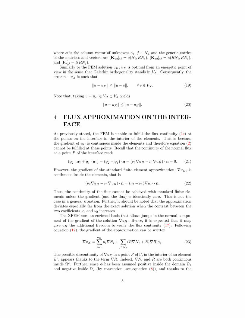
Figure 1: Illustration of (a) the complete domain Ω, the subdomains Ω1 and Ω2

and the interface Γ; (b) zoom on a generic point P of the interface Γ, with thedefinition of the normal and tangent vectors; and (c) description of the interfacewithin an element.

perature distribution over a bi-phasic material: find u such that:

−∇ · q = f in Ω1 ∪ Ω2 (1a)

q = ν∇u in Ω1 ∪ Ω2 (1b)

q · n = gN on ΓN (1c)

u = uD on ΓD (1d)

JqK · n = 0 on Γ (1e)

JuK = 0 on Γ (1f)

In these equations, ν = ν1 in the phase Ω1 and ν = ν2 in the phase Ω2. Thenormal vector n is the outgoing normal vector along ΓN ∪ ΓD and is oriented(arbitrarily) as indicated on figure 1(b), from Ω1 towards Ω2.

Note that the continuity of the (normal) flux, enforced by equation (1e), andthe fact that the material coefficients ν1 and ν2 are different, implies that thegradient of u is necessarily discontinuous (in the direction of the normal to Γ),that is

∇u|Ω1· n 6= ∇u|Ω2

· n. (2)

Note also that the jump of the normal component of the gradient depends onthe contrast between ν1 and ν2. On the contrary, the tangential component ofthe gradient is continuous, due to the continuity of u in Ω. Thus, denoting byτ the unit vector tangent to Γ at P (see figure 1(b)), one has

∇u|Ω1· τ = ∇u|Ω2

· τ . (3)

4

2.1 Variational form

The following functional spaces are introduced to properly state the weak formof the problem. The space V containing the solution u is defined as

V := u ∈ H1(Ω) : u = uD in ΓD, (4)

and the corresponding test functions space, V0 is

V0 := u ∈ H1(Ω) : u = 0 en ΓD. (5)

Thus, the weak form of the problem, equivalent to (1) reads: find u ∈ V suchthat

a(u, v) = `(v), for all v ∈ V0, (6)

where the bilinear and linear forms a(·, ·) and `(·) are given by

a(u, v) :=

∫Ω1∪Ω2

ν∇u · ∇v dΩ and `(v) :=

∫Ω

fv dΩ−∫

ΓN

gNv ds. (7)

It is worth noting that the continuity constraint (1e) is implicitly imposedin (6). In fact, this condition is enforced in (6) in a weak fashion, in the samemanner as the Neumann boundary conditions (1c). Therefore, this restric-tion is exactly fulfilled only if the equation is solved exactly, using the infinite-dimensional spaces V and V0. In the FEM solution, using finite-dimensionalspaces approximating VH and VH0 , these conditions are only verified approxi-mately. We come back to this issue in section 5.

3 PHASE TRACKING WITH LEVEL SETSAND XFEM ENRICHMENT

In this section, we briefly recall the definitions of level sets, of the FEM, andof the XFEM, with a particular emphasis on the type of enrichment functionsthat are used in our version of the XFEM.

3.1 Level sets

Level set functions [36, 37] provide a very efficient and elegant parameterizationof multi-phases domains. In the simplest setting, they allow to discriminatebetween two areas of a domain, with no explicit parameterization of the actualinterface. Conceptually, they are constructed in a space of higher dimensionthan the interface they intend to represent, with a smoother topological behaviorthat allows for an easier manipulation.

The level set is a function φ(x) defined over the entire domain Ω, and itssign indicates the belonging to one or the other of the two areas Ω1 and Ω2:

φ(x) =

> 0, x ∈ Ω1

= 0, x ∈ Γ< 0, x ∈ Ω2

(8)

5

Usually, its absolute value is defined as the distance to the interface. Theinterface is hence parameterized by the set of zeros of the level set.

3.2 Finite Element Method (FEM)

A finite element mesh generates a discrete functional space VH ⊂ V , whereH stands for the characteristic size of the elements in the mesh. The mesh isa partition of the domain Ω into disjoint elements Ωe, e = 1, . . . , ne, that isΩ =

⋃e Ω

eand Ωe ∩Ωe

′= ∅ for e 6= e′. The corresponding discrete counterpart

of the test space V0 is denoted by VH0. The standard FEM basis of shape

functions, generating VH0is denoted by Ni, i = 1, . . . , nH , being nH the number

of nodal points in the finite element mesh.The affine space VH is therefore VH = u?D+VH0 , where u?D is a function in

spanN1, . . . , Npoin, defined over Ω and that coincides with uD on ΓD. Typi-cally, u?D is determined as the interpolation of uD with the FEM mesh. In thefollowing, it is assumed that the FEM discretization properly reproduces uD(no oscillation terms in the data are considered). Thus, the FEM solution uHis defined by the nodal values ui, i = 1, . . . , nH :

uH =

nH∑i=1

Niui, (9)

and is such that

a(uH , v) = `(v), for all v ∈ VH0⊂ V0. (10)

The discretization results in an algebraic system of equations

Kuuu = Fu, (11)

where the unknown column vector u contains the coefficients ui, associated tothe nodes that are not on the Dirichlet boundary ΓD, and the stiffness matrixKuu and force vector Fu have generic components [Kuu]ij = a(Ni, Nj) and[Fu]j = `(Nj)− a(u?D, Nj).

A consequence of the assumption of no data oscillations is that the errorassociated with uH , e := u − uH , belongs to V0. Thus, Galerkin orthogonalityholds and uH is optimal in the sense that

‖u− uH‖ ≤ ‖u− v‖ ∀ v ∈ VH (12)

where ‖ · ‖ is the energy norm, defined by ‖v‖2 = a(v, v).The level set function φ is also approximated by φH ∈ VH and determined

by the nodal values φi, i = 1, . . . , nH ,

φ ≈ φH =

nH∑i=1

Niφi. (13)

6

This allows to describe the interface as a continuous line (surface in 3D), smoothinside the elements and with slope discontinuities when intersecting the elementedges (sides in 3D). For linear triangular elements the interface is a polygonalline.

Thus, the normal vector to the interface (see Figure 1(c)) is easily computedat any point of the interface in the interior of an element Ωe:

n =∇φH‖∇φH‖

with ∇φH =

nH∑i=1

φi∇Ni. (14)

Note that, as φH is positive on Ω1, its gradient, and consequently n, point fromΩ1 towards Ω2.

3.3 EXtended Finite Element Method (XFEM)

The standard FEM provides a solution uH that is infinitely regular (smooth)inside any element Ωe. Therefore, standard finite elements are unable to repro-duce the gradient jumps of the actual solution (see (1e) and (2)). The XFEMenriches the FEM solution using a ridge function, hence enabling the discretiza-tion to introduce a jump of the gradient across the interface. The ridge functionused here is the one introduced in [15] and defined as

R =

nH∑i=1

Ni|φi| −

∣∣∣∣∣nH∑i=1

Niφi

∣∣∣∣∣ . (15)

The function R vanishes in all the elements that are not crossed by the interface.Thus, the support ofR is precisely the set of elements that should be enriched. Inthe following, the set of indices of these elements is denoted by Ea. IntroducingNa as the set of nodal indices corresponding to the nodes belonging to theenriched elements, the previous expression is rewritten as

R =∑i∈Na

Ni|φi| −

∣∣∣∣∣∑i∈Na

Niφi

∣∣∣∣∣ . (16)

For the sake of a simpler notation and without any loss in generality, it isassumed that the enriched nodes are the first in the node list, that is Na =1, 2, . . . , cardNa. Thus, the XFEM approximation, uX , is

uX =

nH∑i=1

Niui +∑j∈Na

RNjaj , (17)

where the coefficients aj , j ∈ Na, stand for the enriched nodal coefficients.The approximation uX lies in the discrete functional space VX = VH ⊕

spanRNi, i ∈ Na and fulfills an equation analogous to (10) but replacing VHby VX . The resulting algebraic linear system of equations reads[

Kuu Kua

KTua Kaa

][u

a

]=

[F u

F a

], (18)

7

where a is the column vector of unknowns aj , j ∈ Na and the generic entriesof the matrices and vectors are [Kua]ij = a(Ni, RNj), [Kaa]ij = a(RNi, RNj),and [Fa]j = `(RNj).

Similarly to the FEM solution uH , uX is optimal from an energetic point ofview in the sense that Galerkin orthogonality stands in VX . Consequently, theerror u− uX is such that

‖u− uX‖ ≤ ‖u− v‖, ∀ v ∈ VX . (19)

Note that, taking v = uH ∈ VH ⊂ VX yields

‖u− uX‖ ≤ ‖u− uH‖. (20)

4 FLUX APPROXIMATION ON THE INTER-FACE

As previously stated, the FEM is unable to fulfill the flux continuity (1e) atthe points on the interface in the interior of the elements. This is becausethe gradient of uH is continuous inside the elements and therefore equation (2)cannot be fulfilled at these points. Recall that the continuity of the normal fluxat a point P of the interface reads

(q2 · n2 + q1 · n1) = (q2 − q1) ·n = (ν2∇uH − ν1∇uH) · n = 0. (21)

However, the gradient of the standard finite element approximation, ∇uH , iscontinuous inside the elements, that is

(ν2∇uH − ν1∇uH) · n = (ν2 − ν1)∇uH · n. (22)

Thus, the continuity of the flux cannot be achieved with standard finite ele-ments unless the gradient (and the flux) is identically zero. This is not thecase in a general situation. Further, it should be noted that the approximationdeviates especially far from the exact solution when the contrast between thetwo coefficients ν1 and ν2 increases.

The XFEM uses an enriched basis that allows jumps in the normal compo-nent of the gradient of the solution ∇uH . Hence, it is expected that it maygive uH the additional freedom to verify the flux continuity (17). Followingequation (17), the gradient of the approximation can be written:

∇uX =

nH∑i=1

ui∇Ni +∑j∈Na

(R∇Nj +Nj∇R)aj . (23)

The possible discontinuity of ∇uX in a point P of Γ, in the interior of an elementΩe, appears thanks to the term ∇R. Indeed, ∇Ni and R are both continuousinside Ωe. Further, since φ has been assumed positive inside the domain Ω1

and negative inside Ω2 (by convention, see equation (8)), and thanks to the

8

definition of R in equation (16), we have the following expressions for R onboth sides of the interface:

R|Ω1=∑i∈Na

Ni (|φi| − φi) and R|Ω2=∑i∈Na

Ni (|φi|+ φi) . (24)

Note that∇R|Ω2−∇R|Ω1

= 2∇φH 6= 0, where φH denotes the level set function,as defined in equation (13). As expected, the jump in the gradient of R is parallelto the normal n, since the latter is parallel to ∇φH . Thanks to this additionalfreedom with respect to the classical finite element approximation, it is expectedthat the XFEM approximation may perform substantially better than the FEM.

In the rest of this section, we illustrate the behavior of the XFEM in termsof global error and quality of the approximation of the fluxes in the vicinityof the interface. We therefore present two simple examples: a square with ahorizontal interface (intersecting the elements of the mesh), and the same witha tilted interface. In the first example, the XFEM captures the exact solutionwhile the FEM behaves poorly. In the second example, the XFEM behaves wellin terms of global error, but the fluxes are wrongly evaluated.

Exemple 1a (horizontal interface): Let us consider the problem (1), withthe following parameters: Ω = [−1, 1]× [−1, 1], gN = 0 for x = ±1, uD = 1 fory = 1, uD = 0 for y = −1, f = 0, ν1 = 1000 and ν2 = 1. Note that the ratioof conductivities is very large. We first consider a perfectly horizontal interface,at y = 0.1 (cutting the elements of the proposed mesh), with Ω2 at y > 0.1. Inthis first configuration, the problem is quasi-1D. The exact solution is:

u(x, y) =1

1100, 9

1000 (y + 1) for y ≤ 0.1

y + 1099, 9 for y > 0.1. (25)

Since the solution is linear, if the mesh were to follow the interface, the FEMsolution would be the exact one. However, in the case that we are interestedin, the interface goes through the elements, and we can observe on figure 2 thatthe solution in terms of fluxes is rather inaccurate. More precisely, because thegradient of the FEM solution is continuous and the contrast in conductivitiesis very large, the fluxes appear to almost cancel on one side of the interface inthe elements that are cut. Hence it appears that there are two jumps in thefluxes: one over the interface, created purely by jump in conductivities; andone between the line of elements cut by the interface and the next one, onlyon the weak side (where ν = 1). On the other side, this discontinuity betweenthe elements cut by the interface and the first line perfectly included inside aphase is not so obvious. These last two remarks are related to the fact that,because it is not using a functional basis that incorporates information on theinterface, the FEM effectively sees an average value of the conductivity ratherthan two phases. As the contrast if very large, this average conductivity is closeto ν1 = 1000, even for elements almost entirely contained in Ω2. Finally, it isimportant to understand that this local quantity of interest will not necessarily

9

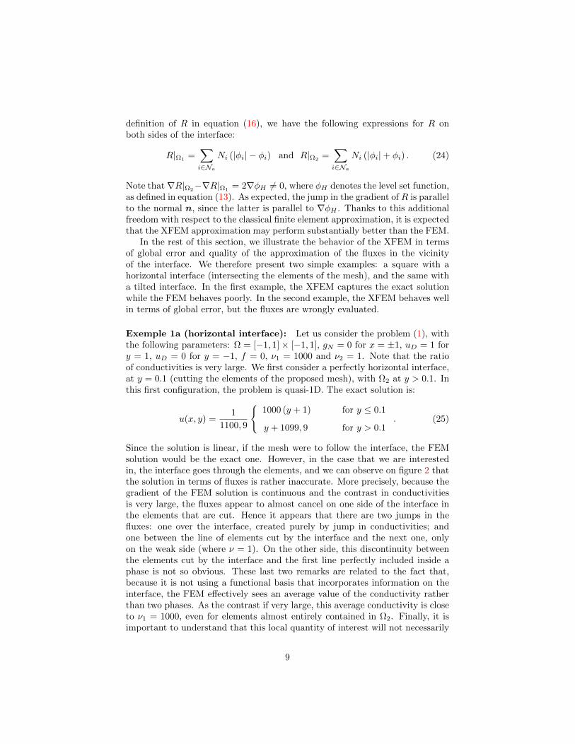
(a) FEM solution, ‖uFEM‖ = 1.997 (b) XFEM solution, ‖uXFEM‖ = 1.816

Figure 2: Example 1a (horizontal interface): the XFEM (right figure) performsbetter than the FEM (left figure) both in terms of global energy norm and localfluxes. The fluxes are evaluated at the Gauss points of each element and drawnin bold for the elements that are cut by the interface.

be better estimated with a more refined mesh. The global approximation willbecome better, but very locally, these two discontinuities will still be observed.On this first configuration, on the other hand, the XFEM captures the analyticalsolution. Indeed, the enriched basis includes the exact solution. Note thatthe comparison between FEM and XFEM is fairly performed in terms of theapproximation properties of the discrete functional spaces. The integrationof the elementary matrices and vectors is therefore performed using the samequadrature. In that sense, the version of FEM used here is nonstandard becauseit also splits the multiphase elements for integration purposes in order to obtainthe stiffness matrix and the force vectors with the same accuracy as the onestypically obtained with XFEM.

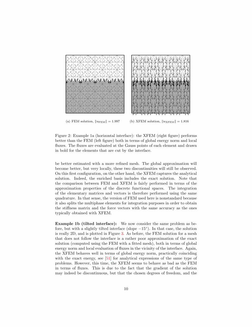
Example 1b (tilted interface): We now consider the same problem as be-fore, but with a slightly tilted interface (slope −15). In that case, the solutionis really 2D, and is plotted in Figure 3. As before, the FEM solution for a meshthat does not follow the interface is a rather poor approximation of the exactsolution (computed using the FEM with a fitted mesh), both in terms of globalenergy norm and local evaluation of fluxes in the vicinity of the interface. Again,the XFEM behaves well in terms of global energy norm, practically coincidingwith the exact energy, see [51] for analytical expressions of the same type ofproblems. However, this time, the XFEM seems to behave as bad as the FEMin terms of fluxes. This is due to the fact that the gradient of the solutionmay indeed be discontinuous, but that the chosen degrees of freedom, and the

10

(a) FEM solution, ‖uFEM‖ = 2.237 (b) XFEM solution, ‖uXFEM‖ = 1.892

Figure 3: Example 1b (tilted interface): the additional degrees of freedom in theXFEM (right figure) induce an improvement with respect to the FEM solution(left figure), in terms of the global energy norm, but not necessarily an improvedevaluation of the fluxes close to the interface.

corresponding functional basis, do not allow to fix the gradients independentlyon each side of the interface. There is an additional freedom with respect to theFEM, but the exact solution is not necessarily contained in the approximatingfunctional space. When the contrast in conductivity becomes large, large varia-tions in the fluxes close to the interface can happen with small variations of themesh.

5 Explicitly Enforcing Flux Continuity

We come back in this section to the way the flux continuity is enforced in theFEM and XFEM and propose to enforce it explicitly to improve the numericalresults in terms of fluxes.

5.1 Weak approximation of Neumann Boundary Condi-tions and flux continuity on the interface

The interface condition (1e) is weakly enforced, in the same fashion as the Neu-mann B.C. (1c). Recall that, when integrating by parts the weighted residualof (1a), the term including the flux on ΓN ,∫

ΓN

ν∇u·nv ds is replaced by

∫ΓN

gNv ds

11

using (1c). In a similar way, integrating by parts in Ω1 and Ω2 and adding twoexpressions, a flux jump term appears in the integral form∫

Γ

(q2 − q1) · n v dΓ (26)

that is readily taken as 0 attending to (1e). The numerical flux on ΓN convergesasymptotically to gN as h tends to zero. The discrete approximation of the fluxesis such that equilibrium is reached in the discrete form, for the sum of the nodalversions of the body loads f and the surface loads gN . Thus, for a given mesh,the numerical flux on ΓN may be a poor approximation to gN , that is, it doesnot fit the data. The same occurs with the flux jump on Γ and, consequently,with the values of q1 ·n and q2 ·n which are, in practice, far from being accurateapproximations.

5.2 Enforcing the flux continuity explicitly

In order to improve the quality of the fluxes on Γ, we propose to enforce explicitlythe weak condition of continuity. That is, we propose to add the followingcondition to the XFEM solution, uX ,

b(µ, uX) = 0, for all µ ∈ VH , (27)

where VH is a discrete space of weighting functions, that has to be chosen, and

b(µ, u) :=

∫Γ

(q2 − q1) · nµdΓ =

∫Γ

(ν2∇u|Ω2− ν1∇u|Ω1

)·nµdΓ. (28)

Note that the weighting functions µ should belong to L2(Γ).With this additional constraint, the flux continuity (1e) is expected to be

fulfilled more accurately because it is not anymore competing with the residualcoming from the interior of the domain.

The condition (27) is added to the original weak form (6) (or its discretecounterpart (10)) using the Lagrange multipliers approach. Thus, the resultingmixed problem reads: find uX ∈ VX and λH ∈ VH such that

a(uX , w) + b(λH , w) = `(w) ∀w ∈ VX,0 (29a)

b(µ, uX) = 0 ∀µ ∈ VH (29b)

The matrix form of (29) results in an enlarged algebraic system of linearequations Kuu Kua Ru

KTua Kaa Ra

RTu RT

a 0

uaλ

=

FuFa0

(30)

where the matrices Ru and Ra are defined below.The Lagrange multipliers space VH must be chosen with care. If its dimen-

sion is too small, the flux continuity condition may be not be enforced strongly

12

a

b

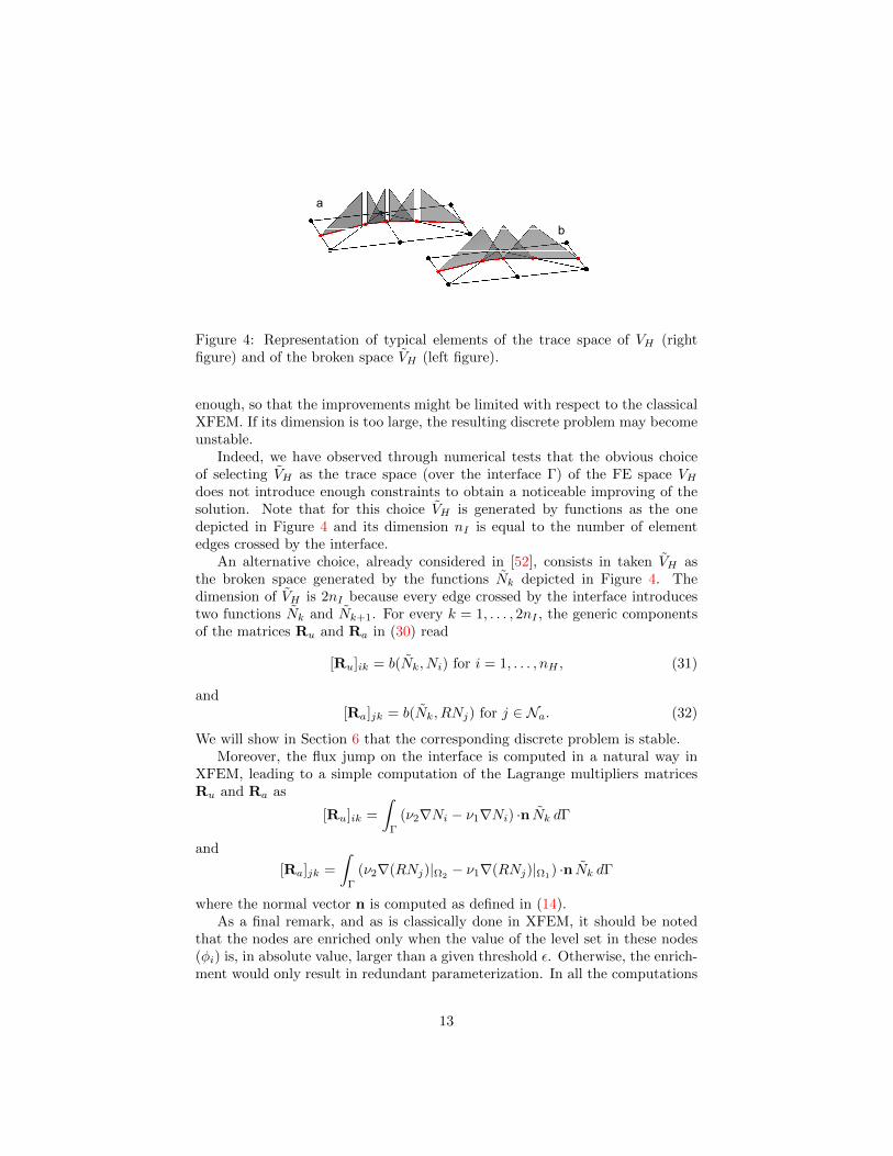
Figure 4: Representation of typical elements of the trace space of VH (rightfigure) and of the broken space VH (left figure).

enough, so that the improvements might be limited with respect to the classicalXFEM. If its dimension is too large, the resulting discrete problem may becomeunstable.

Indeed, we have observed through numerical tests that the obvious choiceof selecting VH as the trace space (over the interface Γ) of the FE space VHdoes not introduce enough constraints to obtain a noticeable improving of thesolution. Note that for this choice VH is generated by functions as the onedepicted in Figure 4 and its dimension nI is equal to the number of elementedges crossed by the interface.

An alternative choice, already considered in [52], consists in taken VH asthe broken space generated by the functions Nk depicted in Figure 4. Thedimension of VH is 2nI because every edge crossed by the interface introducestwo functions Nk and Nk+1. For every k = 1, . . . , 2nI , the generic componentsof the matrices Ru and Ra in (30) read

[Ru]ik = b(Nk, Ni) for i = 1, . . . , nH , (31)

and[Ra]jk = b(Nk, RNj) for j ∈ Na. (32)

We will show in Section 6 that the corresponding discrete problem is stable.Moreover, the flux jump on the interface is computed in a natural way in

XFEM, leading to a simple computation of the Lagrange multipliers matricesRu and Ra as

[Ru]ik =

∫Γ

(ν2∇Ni − ν1∇Ni) ·n Nk dΓ

and

[Ra]jk =

∫Γ

(ν2∇(RNj)|Ω2− ν1∇(RNj)|Ω1

) ·n Nk dΓ

where the normal vector n is computed as defined in (14).As a final remark, and as is classically done in XFEM, it should be noted

that the nodes are enriched only when the value of the level set in these nodes(φi) is, in absolute value, larger than a given threshold ε. Otherwise, the enrich-ment would only result in redundant parameterization. In all the computations

13

performed in this paper, the threshold has been set to ε = 0.05, relative toa characteristic size of the smallest element of the mesh. On the other hand,it has been observed in the numerical experiments that normalizing functionsNk in the broken space VH , for instance enforcing a unitary slope as in someimplementations of the classical finite elements, does not bring a substantialimprovement of the condition number of the global matrix.

6 Stability analysis

The method of Lagrange multipliers leads to a saddle-point problem. The inf-sup condition (or LBB) states [53] that the resulting formulation is stable ifthere exists a k > 0, independent of the mesh size, such that

infµ∈VH

supv∈VX

b(µ, v)

||µ||VH||v||VX

≥ k (33)

Note that the two norms in the denominator are different one from the other.One is defined over the domain Ω while the other is defined over the interfaceΓ.

It is often difficult to prove analytically that the LBB condition is fulfilled. Inappendix A, we give one sketch of such proof of stability. However, as it is basedon some strong hypotheses, that are difficult to prove in practice, we concen-trate in this section on the Chapelle-Bathe test [29] that consists in solving theeigenvalue problem for a series of meshes and showing the boundedness of thesmallest eigenvalue. Passing the numerical test does not guarantee stability butexperience shows that it is very sensitive, and indeed manages to discriminatebetween stable and unstable problems.

The functions µ(x) ∈ VH and v(x) ∈ VX can be written as vector productsµ(x) = N(x)Tµ and v = N(x)Tv, where N and N are vectors of the respectiveinterpolation functions. The length (number of terms) of vector N is nx =nH + cardNa = dimVX and the length of N is 2nI . Their generic terms read:[N(x)]i = Ni(x), for 1 ≤ i ≤ 2nI , [N(x)]i = Ni(x), for 1 ≤ i ≤ nH , and[N(x)]nH+i = R(x)Ni(x), for i ∈ Na, and where µ and v are the vectors of thenodal values of the functions. The matrix form of the operator b(µ, v) in (33)can then be expressed as

b(µ, v) =

∫Γint

µ Jν∇v · nKdΓ = µTRv (34)

where R = [RTu RT

a ] is a 2nI×nx rectangular matrix, whose blocks are defined inEquation (31). Assuming that, for every possible Lagrange multiplier µ ∈ VH ,there exists a solution w ∈ VX , such that µ = Jν∇w · nK, we introduce thematrix J such that µ = Jw. This matrix J = [JTu JTa ] represents the fluxjump operator in the bases N and N. The general term [J]ij is such that∑2nI

j=1 [Ju]ijNj = Jν∇Ni ·nK for 1 ≤ i ≤ nH , and∑2nI

j=1 [Ja]ijNj = Jν∇(RNi)·nKfor i ∈ Na. We note that

R = MµJ (35)

14

−2 −1.5 −1 −0.5 0−2

0

2

4

log10(h)

log 1

0( )

Figure 5: Chapelle-Bathe test: evolution of the smallest eigenvalue as a functionof the size of the mesh.

where Mµ is a mass matrix (corresponding to the L2 product) for the elements

of VH , with general term [Mµ]ij =∫

ΓintNiNjdΓ. We then obtain the discretized

LBB condition:

infw∈R2nx

supv∈R2nx

wTJTMµJv

(wTJTMµJw)1/2

(vTMvv)1/2≥ k, (36)

where Mv is the mass matrix for VX . Note that all the norms are equivalenthere, and we chose the L2 norms for both || · ||VH

and || · ||VX. The Chapelle-

Bathe numerical test [29] consists in checking with numerical experiments theboundedness (from below) of the smallest non-zero eigenvalue of the generalizedeigenvalue problem: find w ∈ R2nx and λ ∈ R such that(

JTMµJ)w = λMvw. (37)

We therefore have to compute the smallest non-zero eigenvalue for a series ofdiscretizations of the same domain with increasingly smaller elements. If thatvalue does not appear to vanish for refined meshes, the test is considered passed.

We consider for the test the Example 1b, described in Section 4 (see alsoFigure 6 for the solution obtained with our approach). The results are plottedin Figure 5 and indeed indicate that the test is passed.

7 Numerical examples

The examples of Section 4 show that, even in very simple scenarios, the FEMintroduces a jump in the flux across the interface. Less intuitively, these exam-ples show that the XFEM solution presents continuous fluxes over the interfaceonly when the flux is orthogonal to the interface (see Figures 2 and 3). In thissection, we first show that our method works well for Example 1b. We thencompare the behavior of our method to the FEM and XFEM solutions in thecase of an unstructured grid. Finally, we describe the convergence of the solu-tions obtained with the three methods in terms of the norm of the flux along theinterface. This convergence study is performed for a problem with analyticalsolution. For easier reference in the remainder of this section, we denote ourmethod by XFEM+.

15

(a) XFEM+ solution, ‖uXFEM+‖ = 1.900

0 0.5 1 1.5 2

2040

0 0.5 1 1.5 2−10

01020

0 0.5 1 1.5 2

−10

0

x 10−13

60

(b) Flux jump along the interface

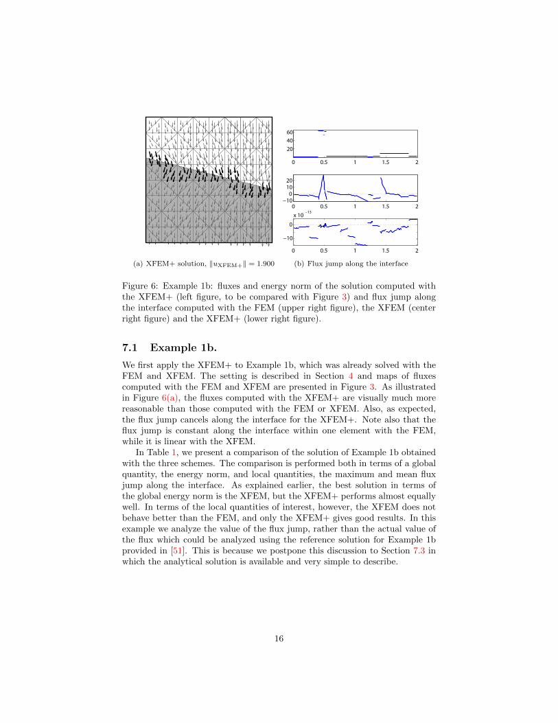
Figure 6: Example 1b: fluxes and energy norm of the solution computed withthe XFEM+ (left figure, to be compared with Figure 3) and flux jump alongthe interface computed with the FEM (upper right figure), the XFEM (centerright figure) and the XFEM+ (lower right figure).

7.1 Example 1b.

We first apply the XFEM+ to Example 1b, which was already solved with theFEM and XFEM. The setting is described in Section 4 and maps of fluxescomputed with the FEM and XFEM are presented in Figure 3. As illustratedin Figure 6(a), the fluxes computed with the XFEM+ are visually much morereasonable than those computed with the FEM or XFEM. Also, as expected,the flux jump cancels along the interface for the XFEM+. Note also that theflux jump is constant along the interface within one element with the FEM,while it is linear with the XFEM.

In Table 1, we present a comparison of the solution of Example 1b obtainedwith the three schemes. The comparison is performed both in terms of a globalquantity, the energy norm, and local quantities, the maximum and mean fluxjump along the interface. As explained earlier, the best solution in terms ofthe global energy norm is the XFEM, but the XFEM+ performs almost equallywell. In terms of the local quantities of interest, however, the XFEM does notbehave better than the FEM, and only the XFEM+ gives good results. In thisexample we analyze the value of the flux jump, rather than the actual value ofthe flux which could be analyzed using the reference solution for Example 1bprovided in [51]. This is because we postpone this discussion to Section 7.3 inwhich the analytical solution is available and very simple to describe.

16

scheme FEM XFEM XFEM+global energy norm 2.237 1.892 1.900

max flux jump 66.3 37.06 1.84e-12mean flux jump 13.4 5.0 4.4e-13

Table 1: Example 1b: comparison, in terms of global energy norm, maximumand minimum flux jumps (in absolute value) of the solutions obtained with thethree schemes.

scheme FEM XFEM XFEM+global energy norm 1.924 1.824 1.824

max flux jump 5.5 4.22 3.9e-12mean flux jump 2.4 0.5 1.4e-12

Table 2: Unstructured mesh example: comparison, in terms of global energynorm, maximum and minimum flux jumps (in absolute value) of the solutionsobtained with the three schemes.

7.2 Unstructured meshes

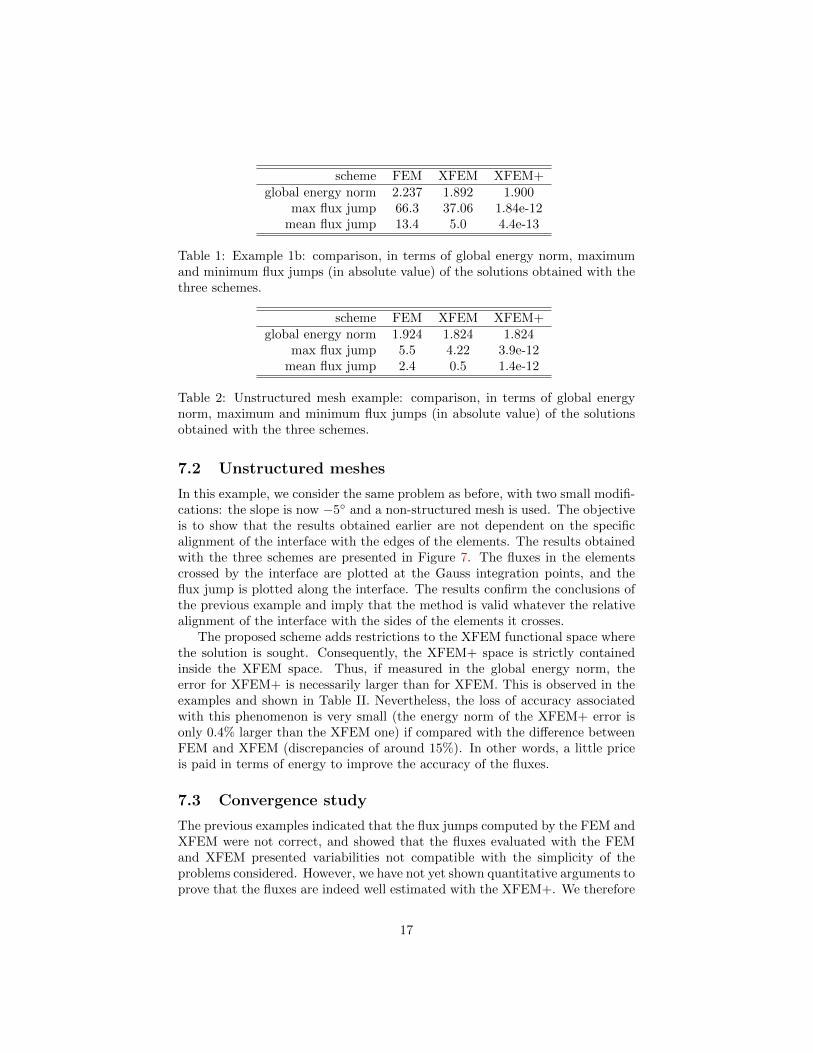
In this example, we consider the same problem as before, with two small modifi-cations: the slope is now −5 and a non-structured mesh is used. The objectiveis to show that the results obtained earlier are not dependent on the specificalignment of the interface with the edges of the elements. The results obtainedwith the three schemes are presented in Figure 7. The fluxes in the elementscrossed by the interface are plotted at the Gauss integration points, and theflux jump is plotted along the interface. The results confirm the conclusions ofthe previous example and imply that the method is valid whatever the relativealignment of the interface with the sides of the elements it crosses.

The proposed scheme adds restrictions to the XFEM functional space wherethe solution is sought. Consequently, the XFEM+ space is strictly containedinside the XFEM space. Thus, if measured in the global energy norm, theerror for XFEM+ is necessarily larger than for XFEM. This is observed in theexamples and shown in Table II. Nevertheless, the loss of accuracy associatedwith this phenomenon is very small (the energy norm of the XFEM+ error isonly 0.4% larger than the XFEM one) if compared with the difference betweenFEM and XFEM (discrepancies of around 15%). In other words, a little priceis paid in terms of energy to improve the accuracy of the fluxes.

7.3 Convergence study

The previous examples indicated that the flux jumps computed by the FEM andXFEM were not correct, and showed that the fluxes evaluated with the FEMand XFEM presented variabilities not compatible with the simplicity of theproblems considered. However, we have not yet shown quantitative arguments toprove that the fluxes are indeed well estimated with the XFEM+. We therefore

17

(a) FEM solution, ‖uFEM‖ = 1.924 (b) XFEM solution, ‖uXFEM‖ = 1.824

(c) XFEM+ solution, ‖uXFEM+‖ = 1.824

0 0.5 1 1.5 2

2

4

0 0.5 1 1.5 2

−2024

0 0.5 1 1.5 2−5

0

5x 10

−12

(d) Flux jump along the interface

Figure 7: Unstructured mesh example: fluxes and energy norm of the solutioncomputed with the three schemes (figures (a), (b) and (c)) and flux jump alongthe interface computed with the FEM ((d), upper figure), the XFEM ((d) centerfigure) and the XFEM+ ((d) lower figure).

18

Ω1

Ω2

Γ

Figure 8: Discretized domain and interface for the convergence study

consider a new problem, for which an analytical solution is known, and computeerrors for the three schemes, in terms of the flux over the interface.

Let us consider the open disc Ω ∈ R2 centered on (0, 0), and with radius 1.It is split into two concentric subdomains Ω1 (disc) and Ω2 (ring) at radius 1/2(see Figure 8). We use cylindrical coordinates (r, θ), and define the parameterν1 = 1000 and ν2 = 1. We finally consider the following problem: find u suchthat

ν∆u+ 4 = 0 , in Ω

u = 0 , at r = 1(38)

with continuity of u and normal flux q = ν∇u · er at the interface r = r0. Theexact solution uex of that problem is given by

uex(r ≤ r0) = r2/1000− 1 + 999/4000,

uex(r ≥ r0) = r2 − 1.(39)

The exact value of the flux, equal in both Ω1 and Ω2 is

ν∇v = 2rer, (40)

so that the exact value of the normal flux along the interface is qex = 2r0

We compute the approximate solution to this problem using five differentmeshes with increasing number of elements and the three different schemes(FEM, XFEM, XFEM+). For each mesh and each scheme we compute therelative error in terms of the flux at the interface as

e =|qex − qh||qex|

, (41)

where qh is the approximate flux, computed on the interface Γ on the side ofΩ2. We then plot in Figure 9 the evolution of that error with the size of theelements. This figure shows that the only method that converges with the size

19

−2 −1.8 −1.6 −1.4 −1.2 −1 −0.8 −0.6−2

−1

0

1

2

3

FE

XFE

XFE+

log h

log

||err

rel||

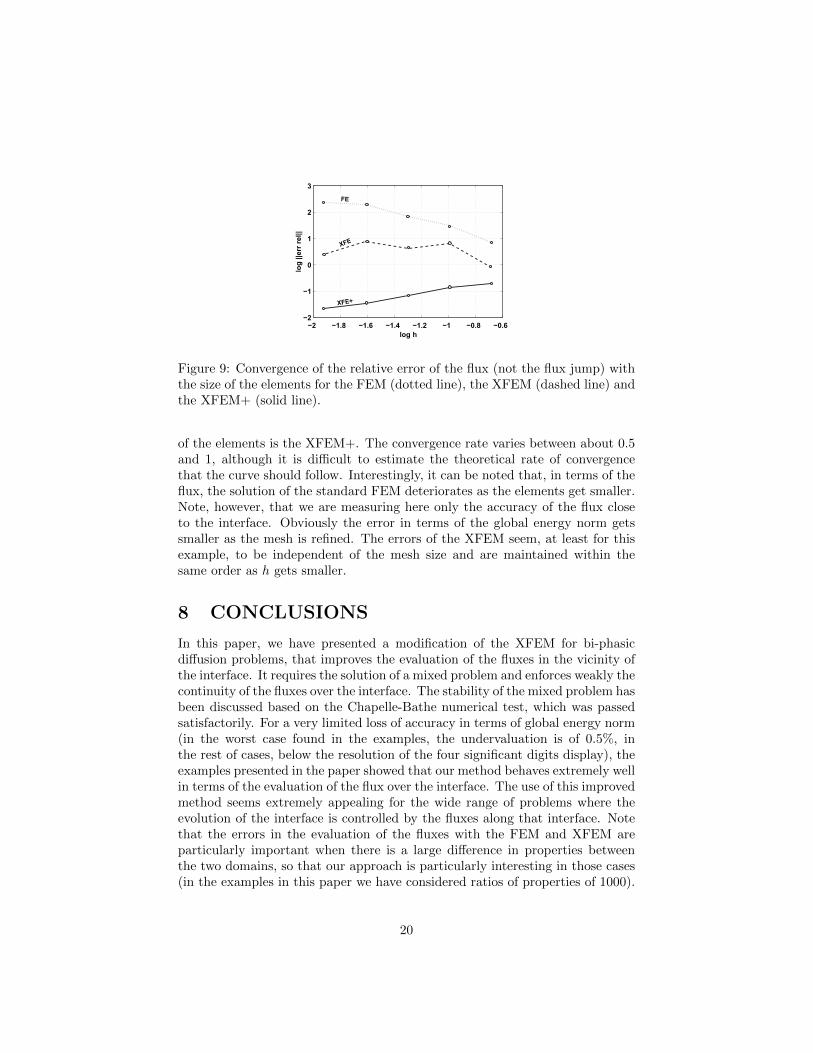
Figure 9: Convergence of the relative error of the flux (not the flux jump) withthe size of the elements for the FEM (dotted line), the XFEM (dashed line) andthe XFEM+ (solid line).

of the elements is the XFEM+. The convergence rate varies between about 0.5and 1, although it is difficult to estimate the theoretical rate of convergencethat the curve should follow. Interestingly, it can be noted that, in terms of theflux, the solution of the standard FEM deteriorates as the elements get smaller.Note, however, that we are measuring here only the accuracy of the flux closeto the interface. Obviously the error in terms of the global energy norm getssmaller as the mesh is refined. The errors of the XFEM seem, at least for thisexample, to be independent of the mesh size and are maintained within thesame order as h gets smaller.

8 CONCLUSIONS

In this paper, we have presented a modification of the XFEM for bi-phasicdiffusion problems, that improves the evaluation of the fluxes in the vicinity ofthe interface. It requires the solution of a mixed problem and enforces weakly thecontinuity of the fluxes over the interface. The stability of the mixed problem hasbeen discussed based on the Chapelle-Bathe numerical test, which was passedsatisfactorily. For a very limited loss of accuracy in terms of global energy norm(in the worst case found in the examples, the undervaluation is of 0.5%, inthe rest of cases, below the resolution of the four significant digits display), theexamples presented in the paper showed that our method behaves extremely wellin terms of the evaluation of the flux over the interface. The use of this improvedmethod seems extremely appealing for the wide range of problems where theevolution of the interface is controlled by the fluxes along that interface. Notethat the errors in the evaluation of the fluxes with the FEM and XFEM areparticularly important when there is a large difference in properties betweenthe two domains, so that our approach is particularly interesting in those cases(in the examples in this paper we have considered ratios of properties of 1000).

20

A Analytical study of stability

The numerical demonstration of stability presented in section 6, based on theideas of [29] is here complemented by a theoretical result. This propositionstates that for the proposed formulation, the LBB condition is proven to hold.This result requires some assumptions that are not obvious to guarantee butthat, in practice, are fulfilled.

The proof is based on one idea already introduced in the numerical test. Forthe selected spaces, it is shown that any function µ in the Lagrange multipliersspace, VH can be recovered as the jump of the normal flux of some function vin VX . Moreover, it is also shown that the norm of v is bounded by above bythe norm of µ.

First, these properties are stated in an element-wise format.

Lemma A.1 (Element-wise property) Let Ωe be one linear triangular ele-ment crossed by the interface Γ. The restriction of Γ to Ωe is denoted Γe. Thenodes of Ωe are denoted P1, P2 and P3, choosing the order such that P1 and P2

are on the same side of the interface. As classically done in XFEM, we assumethat ∃ε > 0 such that |Γe| > ε. The restrictions of the functional spaces VXand VH to Ωe and Γe are denoted V eX and V eH , with their respective L2 norms‖v‖2V e

X=∫

Ωe v2dΩ and ‖µ‖2

V eH

=∫

Γe µ2dΓ. The standard FE shape function

corresponding to the node P1 is denoted N1, and the ridge function, defined atequation (16), is denoted R.

Then ∃α > 0 such that ∀µ ∈ V eH , ∃v ∈ spanN1, RN1 ⊂ V eX (i.e. describingv with the d.o.f. corresponding to P1 only) verifying

1. Jν∇v · nK = µ;

2. ‖v‖V eX≤ α‖µ‖V e

H.

Let us consider a function v = u1N1 + a1N1R ∈ spanN1, RN1, where u1 anda1 are two scalar values. Let us denote by γ1 and γ2 the jumps of the normalfluxes corresponding to N1 and RN1, namely

γ1 := Jν∇N1 · nK and γ2 := Jν∇N1R · nK.

Note that γ1 is a constant function on Γe, which vanishes only if ∇N1 is or-thogonal to n, that is in the case of being Γe perpendicular to the side P2P3 ofthe element. In this case, the node P1 has to be replaced by P2. Function γ2 islinear (not constant) and therefore γ1, γ2 is a basis of V eH . Thus, varying thecoefficients u1 and a1, the jump of v, may reproduce any function µ ∈ V eH , thatis

µ = u1γ1 + a1γ2 = Jν∇v · nK.

Moreover, being both v and µ represented by the coefficients [u1 a1] in the basesN1, N1R and γ1, γ2 respectively, their norms are expressed as

‖v‖2V eX

= [u1 a1]Mv[u1 a1]T and ‖µ‖2V eH

= [u1 a1]Mµ[u1 a1]T,

21

being Mv and Mµ 2× 2 mass matrices with generic terms

[Mv]ij =

∫Ωe

N21R

i+j−2 dΩ and [Mµ]ij =

∫Γe

γiγj dΓ for i, j = 1, 2

The second part of the statement is readily proved by taking α equal to αmax,the maximum eigenvalue of the following generalized eigenvalue problem.

Mvq = αMµq, (42)

The fact that this eigenvalue is bounded from below (it cannot be indefinitelysmall) is guaranteed by the fact that the elements are regular enough and theminimum length of the interface inside the element is also limited.

This bounding property holds for a given value of H. It is necessary tocheck also the tendency of α in the limit case, that is when H tends to 0. Notethat, with respect to the characteristic element size, H, Mv scales with H2

and Mµ scales with H. Therefore, α is expected to scale with H. This is theright tendency for the final result shown in Theorem A.4 because it has to beguaranteed that k is larger than a given value and k is taken as the inverse of α.Thus, taking k equal to the inverse of the α corresponding to Hmax (the largestpossible element size) we are in the safe side.

The next proposition states that the decay of a function v defined in an ele-ment Ωe is fast enough to control the propagation of the norm into the neighborelements.

Lemma A.2 (Bound of the norm propagated to the neighbor elements)Let Ωe and Ωe+1 be two contiguous elements crossed by the interface and P1 P2

and P3 the nodes of Ωe. Then, ∃β > 0 such that, for any v defined by the d.o.f.of Ωe,

v ∈ spanNi, RNi i = 1, 2, 3 (43)

it holds that‖v‖V e+1

X≤ β‖v‖V e

X. (44)

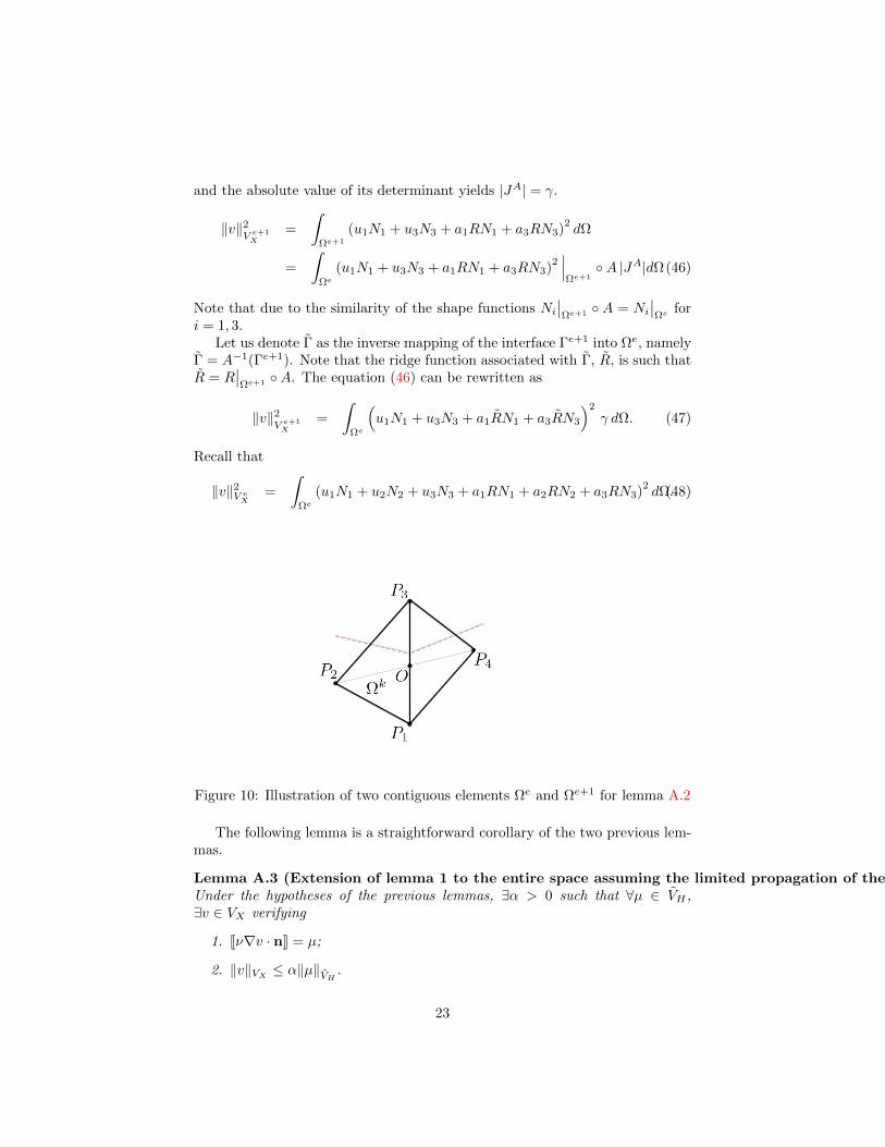
Let us denote P1 and P3 the common nodes to Ωe and Ωe+1, being P2 thethird node in Ωe, see figure 10. P1 is selected such that it is on the same sideof the interface as P2. The third node in Ωe+1 is denoted as P4 as shown inFigure 10. In order to define a mapping transforming Ωe into Ωe+1 we introducethe following: let O be the intersection point of straight lines P1P3 and P2P4,

γ = |OP4||OP2| and θ the angle between OP1 and OP2. Then the affinity, A, of axis

P1P3 following the direction of P2P4 and ratio −γ, maps Ωe into Ωe+1. Selectingthe proper coordinate axis, the Jacobian of the affinity is

JA =

(−γ −γ cot θ0 1

)(45)

22

and the absolute value of its determinant yields |JA| = γ.

‖v‖2V e+1X

=

∫Ωe+1

(u1N1 + u3N3 + a1RN1 + a3RN3)2dΩ

=

∫Ωe

(u1N1 + u3N3 + a1RN1 + a3RN3)2∣∣∣Ωe+1

A |JA|dΩ(46)

Note that due to the similarity of the shape functions Ni∣∣Ωe+1 A = Ni

∣∣Ωe for

i = 1, 3.Let us denote Γ as the inverse mapping of the interface Γe+1 into Ωe, namely

Γ = A−1(Γe+1). Note that the ridge function associated with Γ, R, is such thatR = R

∣∣Ωe+1 A. The equation (46) can be rewritten as

‖v‖2V e+1X

=

∫Ωe

(u1N1 + u3N3 + a1RN1 + a3RN3

)2

γ dΩ. (47)

Recall that

‖v‖2V eX

=

∫Ωe

(u1N1 + u2N2 + u3N3 + a1RN1 + a2RN2 + a3RN3)2dΩ.(48)

Figure 10: Illustration of two contiguous elements Ωe and Ωe+1 for lemma A.2

The following lemma is a straightforward corollary of the two previous lem-mas.

Lemma A.3 (Extension of lemma 1 to the entire space assuming the limited propagation of the functional norms)Under the hypotheses of the previous lemmas, ∃α > 0 such that ∀µ ∈ VH ,∃v ∈ VX verifying

1. Jν∇v · nK = µ;

2. ‖v‖VX≤ α‖µ‖VH

.

23

The following theorem is a direct consequence of the previous lemma andguarantees the fulfillment of the LBB condition.

Theorem A.4 Under the assumptions of regularity of the mesh and of locallength of the interface, ∃k > 0 such that

infµ∈VH

supw∈VH

b(µ,w)

||µ||VH||w||VX

≥ k

For a given µ, take v as indicated in Lemma A.3. Then

b(µ,w) =

∫Γ

µ2dΓ = ||µ||2VH

andb(µ, v)

||µ||VH||v||VX

=||µ||VH

||v||VX

Since ||v||VX≤ α||µ||, taking k = 1/α the proposition follows.

This is equivalent to satisfy the LBB condition and guarantees the stabilityof the scheme.

Support from Ministerio de Educacion y Ciencia, Grant DPI2011-27778-C02-02 is deeply acknowledged.

References

[1] Goldstein D, Handler R, Sirovich L. Modeling a no-slip flow boundarywith an external force field. J. Comp. Phys. 1993; 105(2):354–366, doi:10.1006/jcph.1993.1081.

[2] Angot P, Bruneau CH, Fabrie P. A penalization method to take into ac-count obstacles in incompressible viscous flows. Numerische Mathematik1999; 81(4):497–520, doi:10.1007/s002110050401.

[3] Peskin CS. The immersed boundary method. Acta Numer. 2002; 11:479–517, doi:10.1017/S0962492902000077.

[4] Vennat E, Aubry D, Degrange M. Collagen fiber network infiltration:permeability and capillary infiltration. Transport Porous Media 2010;84(3):717–733, doi:10.1007/s11242-010-9537-4.

[5] Barrett JW, Elliott CM. Fitted and unfitted finite-element methods forelliptic equations with smooth interfaces. IMA J. Numer. Anal. 1987;7(3):283–300, doi:10.1093/imanum/7.3.283.

[6] Mackinnon RJ, Carey GF. Treatment of material discontinuity in finiteelement computations. Int. J. Numer. Meth. Engrg. 1987; 24(2):393–417,doi:10.1002/nme.1620240209.

24

[7] Pehlivanov AI, Lazarov RD, Carey GF, Chow SS. Superconvergence anal-ysis of approximate boundary-flux calculations. Numerische Mathematik1992; 63(1):483–501, doi:10.1007/BF01385871.

[8] Melenk JM, Babuska I. The partition of unity finite element method: basictheory and applications. Comp. Meth. Appl. Mech. Engrg. 1996; 139(1-4):289–314.

[9] Oden JT, Duarte CA, Zienkiewicz OC. A new cloud-based hp finite elementmethod. Comp. Meth. Appl. Mech. Engrg. 1998; 153(1-2):117–126.

[10] Moes N, Dolbow J, Belytschko T. A finite element method for crack growthwithout remeshing. Int. J. Numer. Meth. Engrg. 1999; 46(1):131–150, doi:10.1002/(SICI)1097-0207(19990910)46:1〈131::AID-NME726〉3.0.CO;2-J.

[11] Chessa J, Smolinski P, Belytschko T. The extended finite element method(XFEM) for solidification problems. Int. J. Numer. Meth. Engrg. 2002;53(8):1959–1977, doi:10.1002/nme.386.

[12] Merle R, Dolbow J. Solving thermal and phase change problems with theeXtended finite element method. Comp. Mech. 2002; 28(5):339–350, doi:10.1007/s00466-002-0298-y.

[13] Belytschko T, Parimi C, Moes N, Sukumar N, Usui S. Structured extendedfinite element methods of solids defined by implicit surfaces. Int. J. Numer.Meth. Engrg. 2003; 56(4):609–635, doi:10.1002/nme.686.

[14] Chessa J, Belytschko T. An extended finite element method for two–phasefluids: flow simulation and modeling. J. Appl. Mech. 2003; 70(1):10–17,doi:10.1115/1.1526599.

[15] Moes N, Cloirec M, Cartaud P, Remacle JF. A computational approachto handle complex microstructure geometries. Comp. Meth. Appl. Mech.Engrg. 2003; 192(28-30):3163–3177, doi:10.1016/S0045-7825(03)00346-3.

[16] Dolbow J, Fried E, Ji H. A numerical strategy for investigating the kineticresponse of stimulus-responsive hydrogels. Comp. Meth. Appl. Mech. Engrg.2005; 194(42-44):4447–4480, doi:10.1016/j.cma.2004.12.004.

[17] Duddu R, Bordas S, Chopp D, Moran B. A combined extended finite ele-ment and level set method for biofilm growth. Int. J. Numer. Meth. Engrg.2008; 74(5):848–870, doi:10.1002/nme.2200.

[18] Legrain G, Moes N, Huerta A. Stability of incompressible formulationsenriched with X–FEM. Comp. Meth. Appl. Mech. Engrg. 2008; 197(21-24):1835–1849, doi:10.1016/j.cma.2007.08.032.

[19] Zlotnik S, Dıez P. Hierarchical X-FEM for n-phase flow (n>2). Comp. Meth.Appl. Mech. Engrg. 2009; 198(30-32):2329–2338, doi:10.1016/j.cma.2009.02.025.

25

[20] Fries TP. The intrinsic XFEM for two-fluid flows. Int. J. Numer. Meth.Fluids 2009; 60(4):437–471, doi:10.1002/fld.1901.

[21] Cottereau R, Dıez P, Huerta A. Modeling, with a unified level-set rep-resentation, of the expansion of a hollow in the ground under differ-ent physical phenomena. Comp. Mech. 2010; 46(2):315–327, doi:10.1007/s00466-009-0443-y.

[22] Knapen A, Poesen J, Govers G, Gyssels G, Nachtergaele J. Resistance ofsoils to concentrated flow erosion: a review. Earth-Sci. Rev. 2007; 80(1-2):75–109, doi:10.1016/j.earscirev.2006.08.001.

[23] Hansbo A, Hansbo P. An unfitted finite element method, based on Nitsche’smethod, for elliptic interface problems. Comp. Meth. Appl. Mech. Engrg.2002; 191(47-48):5537–5552, doi:10.1016/S0045-7825(02)00524-8.

[24] Harari I, Dolbow J. Analysis of an efficient finite element method for em-bedded interface problems. Comp. Mech. 2010; 46:205–211, doi:10.1007/s00466-009-0457-5.

[25] Zunino P, Cattaneo L, Colciago CM. An unfitted interface penalty methodfor the numerical approximation of contrast problems. Appl. Numer. Math.2011; doi:10.1016/j.apnum.2011.06.005.

[26] Ji H, Dolbow JE. On strategies for enforcing interfacial constraints andevaluating jump conditions with the extended finite element method. Int.J. Numer. Meth. Engrg. 2004; 61(14):2508–2535, doi:10.1002/nme.1167.

[27] Moes N, Bechet E, Tourbier M. Imposing Dirichlet boundary conditionsin the extended finite element method. Int. J. Numer. Meth. Engrg. 2006;67(12):1641–1669, doi:10.1002/nme.1675.

[28] Bechet E, Moes N, Wohlmuth B. A stable Lagrange multiplier space forstiff interface conditions within the extended finite element method. Int. J.Numer. Meth. Engrg. 2009; 78(8):931–954, doi:10.1002/nme.2515.

[29] Chapelle D, Bathe KJ. The inf-sup test. Comp. & Struct. 1993; 47(4-5):537–545.

[30] Bathe KJ. The inf-sup condition and its evaluation for mixed finite elementmethods. Comp. & Struct. 2001; 79(2):243–252.

[31] Kim TY, Dolbow J, Laursen T. A mortared finite element method forfrictional contact on arbitrary interfaces. Comp. Mech. 2007; 39(3):223–235, doi:10.1007/s00466-005-0019-4.

[32] Crank J. Free and moving boundary problems. Oxford University Press,1984.

26

[33] Unverdi SO, Tryggvason G. A front-tracking method for viscous, in-compressible, multi-fluid flows. J. Comp. Phys. 1992; 100(1):25–37, doi:10.1016/0021-9991(92)90307-K.

[34] Gorczyk W, Gerya TV, Connolly JAD, Yuen DA, Rudolph M.Large–scale rigid–body rotation in the mantle wedge and its implica-tions for seismic tomography. Geochem. Geophys. Geosyst. 2006; 7(5).Doi:10.1029/2005GC001075.

[35] Jan YJ. A cell-by-cell thermally driven mushy cell tracking algorithm forphase-change problems. Comp. Mech. 2007; 40(2):201–216, doi:10.1007/s00466-006-0098-x.

[36] Sethian JA. Level Set Methods and Fast Marching Methods: Evolving Inter-faces in Computational Geometry, Fluid Mechanics, Computer Vision, andMaterials Science. Cambridge University Press: Cambridge, U.K., 1999.

[37] Osher S, Fedkiw R. Level set methods: an overview and some recent results.J. Comp. Phys. 2001; 169(2):463–502, doi:10.1006/jcph.2000.6636.

[38] Osher S, Sethian JA. Fronts propagating with curvature-dependent speed:Algorithms based on Hamilton-Jacobi formulations. J. Comp. Phys. 1988;79(1):12–49, doi:10.1016/0021-9991(88)90002-2.

[39] Sussman M, Smereka P, Osher S. A level set approach for computing solu-tions to incompressible two-phase flow. J. Comp. Phys. 1994; 114(1):146–159, doi:10.1006/jcph.1994.1155.

[40] Mulder W, Osher S, Sethian JA. Computing interface motion in com-pressible gas dynamics. J. Comp. Phys. 1992; 100(2):209–228, doi:10.1016/0021-9991(92)90229-R.

[41] Karlsen KH, Lie KA, Risebro NH. A fast marching method forreservoir simulation. Comp. Geosci. 2000; 4(2):185–206, doi:10.1023/A:1011564017218.

[42] Nielsen LK, Li H, Tai XC, Aanonsen SI, Espedal M. Reservoir descrip-tion using a binary level set model. Comp. Visu. Sci. 2008; doi:10.1007/s00791-008-0121-1.

[43] Zlotnik S, Dıez P, Fernandez M, Verges J. Numerical modelling of tectonicplates subduction using X–FEM. Comp. Meth. Appl. Mech. Engrg. 2007;196(41-44):4283–4293, doi:10.1016/j.cma.2007.04.006.

[44] Zlotnik S, Fernandez M, Dıez P, Verges J. Modelling gravitational insta-bilities: slab break-off and Rayleigh-Taylor diapirism. Pure Appl. Geophys.2008; 165:1–20, doi:10.1007/s00024-004-0386-9.

[45] Sethian JA, Popovici AM. 3-D traveltime computation using the fastmarching method. Geophys. 1999; 64(2):516–523, doi:10.1190/1.1444558.

27

[46] Ito K, Kunisch K, Li Z. Level-set function approach to an inverse interfaceproblem. Inverse Prob. 2001; 17(5):1225–1242, doi:10.1088/0266-5611/17/5/301.

[47] Burger M. A level set method for inverse problems. Inverse Prob. 2001;17(5):1327–1355, doi:10.1088/0266-5611/17/5/307.

[48] Burger M, Osher SJ. A survey of level set methods for inverse problems andoptimal design. Europ. J. Appl. Math. 2005; 16(2):263–301, doi:10.1017/S0956792505006182.

[49] Cordero F, Dıez P. XFEM+: una modificacion de XFEM para mejorar laprecision de los flujos locales en problemas de difusion con conductividadesmuy distintas. Revista Internacional Metodos Numericos para Calculo yDiseno en Ingenierıa 2010; 26(2):121–133.

[50] Cottereau R, Dıez P. Numerical modeling of erosion using an improvementof the extended finite element method. Europ. J. Environmental Civil En-grg. 2011; 15(8):1187–1206, doi:10.3166/EJECE.15.1187-1206.

[51] Legrain G, Allais R, Cartraud P. On the use of the extended finite elementmethod with quadtree/octree meshes. Int. J. Numer. Meth. Engrg.. 2011;86:717–743.

[52] Soghrati S, Aragon AM, Duarte CA, Geubelle PH. An interface-enrichedgeneralized FEM for problems with discontinuous gradient fields. Int. J.Numer. Meth. Engrg. 2012; 89(8):991–1008.

[53] Brezzi F. On the existence, uniqueness and approximation of saddle-point problems arising from lagrangian multipliers. Revue Francaised’Automatique, Informatique et Recherche Operationnelle 1974; 8(2):129–151.

28