A Spectral Learning Approach to Range-Only SLAM

Byron Boots bboots@cs.washington.edu

Department of Computer Science and Engineering, University of Washington, Seattle, WA

Geo↵rey J. Gordon ggordon@cs.cmu.edu

Machine Learning Department, Carnegie Mellon University, Pittsburgh, PA 15213

AbstractWe present a novel spectral learning algo-rithm for simultaneous localization and map-ping (SLAM) from range data with knowncorrespondences. This algorithm is an in-stance of a general spectral system identifi-cation framework, from which it inherits sev-eral desirable properties, including statisti-cal consistency and no local optima. Com-pared with popular batch optimization ormultiple-hypothesis tracking (MHT) meth-ods for range-only SLAM, our spectral ap-proach o↵ers guaranteed low computationalrequirements and good tracking performance.Compared with MHT and with popular ex-tended Kalman filter (EKF) or extended in-formation filter (EIF) approaches, our ap-proach does not need to linearize a transi-tion or measurement model. We provide atheoretical analysis of our method, includ-ing finite-sample error bounds. Finally, wedemonstrate on a real-world robotic SLAMproblem that our algorithm is not only the-oretically justified, but works well in prac-tice: in a comparison of multiple methods,the lowest errors come from a combination ofour algorithm with batch optimization, butour method alone produces nearly as good aresult at far lower computational cost.

1. IntroductionIn range-only SLAM, we are given a sequence of rangemeasurements from a robot to fixed landmarks withknown correspondences, and possibly a matching se-quence of odometry measurements. We then attemptto simultaneously estimate the robot’s trajectory and

Proceedings of the 30 th International Conference on Ma-chine Learning, Atlanta, Georgia, USA, 2013. JMLR:W&CP volume 28. Copyright 2013 by the author(s).

the locations of the landmarks. Popular approachesto range-only SLAM include EKFs and EIFs (Kantor& Singh, 2002; Kurth et al., 2003; Djugash & Singh,2008; Djugash, 2010; Thrun et al., 2005), multiple-hypothesis trackers (including particle filters and mul-tiple EKFs/EIFs) (Djugash et al., 2005; Thrun et al.,2005), and batch optimization of a likelihood func-tion (Kehagias et al., 2006).

In all the above approaches, the most popular repre-sentation for a hypothesis is a list of landmark loca-tions (mn,x,mn,y) and a list of robot poses (xt, yt, ✓t).Unfortunately, both the motion and measurementmodels are highly nonlinear in this representation,leading to computational problems: inaccurate lin-earizations in EKF/EIF/MHT and local optima inbatch optimization approaches. Much work has at-tempted to remedy this problem, e.g., by changing thehypothesis representation (Djugash, 2010) or by keep-ing multiple hypotheses (Djugash et al., 2005; Dju-gash, 2010; Thrun et al., 2005). While considerableprogress has been made, none of these methods areideal; common di�culties include the need for an ex-tensive initialization phase, inability to recover frompoor initialization, lack of performance guarantees, orexcessive computational requirements.

We take a very di↵erent approach: we formulate range-only SLAM as a matrix factorization problem, wherefeatures of observations are linearly related to a 4- or7-dimensional state space. This approach has severaldesirable properties. First, we need weaker assump-tions about the measurement model and motion modelthan previous approaches to SLAM. Second, our statespace yields a linear measurement model, so we loseless information during tracking to approximation er-rors and local optima. Third, our formulation leads toa simple spectral learning algorithm, based on a fastand robust singular value decomposition (SVD)—infact, our algorithm is an instance of a general spectralsystem identification framework, from which it inherits

A Spectral Learning Approach to Range-Only SLAM

desirable guarantees including statistical consistencyand no local optima. Fourth, we don’t need to worryas much as previous methods about errors such as aconsistent bias in odometry, or a receiver mounted ata di↵erent height from the transmitters: in general,we can learn to correct such errors automatically byexpanding the dimensionality of our state space.

As we will discuss in Section 2, our approach to SLAMhas much in common with spectral algorithms for sub-space identification (Van Overschee & De Moor, 1996;Boots et al., 2010); unlike these methods, our focus onSLAM makes it easy to interpret our state space. Ourapproach is also related to factorization-based struc-ture from motion (Tomasi & Kanade, 1992; Triggs,1996; Kanade & Morris, 1998), as well as to recentdimensionality-reduction-based methods for localiza-tion and mapping (Biggs et al., 2005; Ferris et al.,2007; Yairi, 2007). Unlike the latter approaches, whichare generally nonlinear, we only require linear dimen-sionality reduction. Finally, the simplest version ofour method (Sec. 3.1) is related to multidimensionalscaling (MDS). In MDS, there is no distinction be-tween landmark positions and robot positions: we haveall-to-all range measurements for a set of landmarks,and must recover an embedding of the landmarks.Our smaller set of measurements introduces additionalchallenges, and forces changes compared to MDS.

2. BackgroundThere are three main pieces of relevant background:first, the well-known solutions to range-only SLAM us-ing variations of the extended Kalman filter and batchoptimization; second, recently-discovered spectral ap-proaches to identifying parameters of nonlinear dy-namical systems; and third, matrix factorization forfinding structure from motion in video. Below, wewill discuss the connections between these areas, andshow how they can be unified within a spectral learn-ing framework.

2.1. Likelihood-based Range-only SLAMThe standard probabilistic model for range-only lo-calization (Kantor & Singh, 2002; Kurth et al., 2003)represents robot state by a vector st = [xt, yt, ✓t]T; therobot’s (nonlinear) motion and observation models are

st+1

=

2

4xt + vt cos(✓t)yt + vt sin(✓t)

✓t + !t

3

5+ ✏t (1)

dt,n =q

(mn,x � xt)2 + (mn,y � yt)2 + ⌘t (2)

Here vt is the distance traveled, !t is the orientationchange, dt,n is the estimate of the range from the nthlandmark location (mn,x,mn,y) to the current location

of the robot (xt, yt), and ✏t and ⌘t are noise. (Through-out this paper we assume known correspondences,since range sensing systems such as radio beaconstypically associate unique identifiers with each read-ing.) To handle SLAM rather than just localization,we extend the state to include landmark positions:

st = [xt, yt, ✓t,m1,x,m1,y, . . . ,mN,x,mN,y]T (3)

where N is the number of landmarks. The motionand measurement models remain the same. Giventhis model, we can use any standard optimization al-gorithm (such as Gauss-Newton) to fit the unknownrobot and landmark parameters by maximum likeli-hood. Or, we can track these parameters online usingEKFs, EIFs, or MHT methods like particle filters.

EKFs and EIFs are a popular solution for localiza-tion and mapping problems: for each new odometryinput at = [vt,!t]T and each new measurement dt, wepropagate the estimate of the robot state and error co-variance by linearizing the non-linear motion and mea-surement models. Unfortunately, though, range-onlySLAM is notoriously di�cult for EKFs/EIFs: sincerange-only sensors are not informative enough to com-pletely localize a robot or a landmark from a smallnumber of readings, nonlinearities are much worse inrange-only SLAM than they are in other applicationssuch as range-and-bearing SLAM. In particular, if wedon’t have a sharp prior distribution for landmark po-sitions, then after a few steps, the exact posterior be-comes highly non-Gaussian and multimodal; so, anyGaussian approximation to the posterior is necessarilyinaccurate. Furthermore, an EKF will generally noteven produce the best possible Gaussian approxima-tion: a good linearization would tell us a lot aboutthe modes of the posterior, which would be equiva-lent to solving the original SLAM problem. So, prac-tical applications of the EKF to range-only SLAMattempt to delay linearization until enough informa-tion is available, e.g., via an extended initializationphase for each landmark. Finally, Djugash et al. pro-posed a polar parameterization to more accurately rep-resent the annular and multimodal distributions typ-ically encountered in range-only SLAM. The result-ing approach is called the ROP-EKF, and is shown tooutperform the ordinary (Cartesian) EKF in severalreal-world problems, especially in combination withmultiple-hypothesis tracking (Djugash & Singh, 2008;Djugash, 2010). However, the multi-hypothesis ROP-EKF can be much more expensive than an EKF, andis still a heuristic approximation to the true posterior.

2.2. Spectral System IdentificationSystem identification algorithms attempt to learn dy-namical system parameters such as a state space, a

A Spectral Learning Approach to Range-Only SLAM

dynamics model (motion model), and an observationmodel (measurement model) directly from samples ofobservations and actions. In the last few years, spec-tral system identification algorithms have become pop-ular; these algorithms learn a state space via a spec-tral decomposition of a carefully designed matrix ofobservable features, then find transition and observa-tion models by linear regressions involving the learnedstates. Originally, subspace identification algorithmswere almost exclusively used for linear system iden-tification (Van Overschee & De Moor, 1996), but re-cently, similar spectral algorithms have been used tolearn models of partially observable nonlinear dynam-ical systems such as HMMs (Hsu et al., 2009; Siddiqiet al., 2010) and PSRs (Rosencrantz et al., 2004; Bootset al., 2010; Boots & Gordon, 2010; Boots et al., 2011).This is a powerful and appealing approach: the result-ing algorithms are statistically consistent, unlike thepopular expectation maximization (EM) algorithm,and they are easy to implement with e�cient linearalgebra operations. As we will see in Section 3, wecan view the range-only SLAM problem as an instanceof spectral state space discovery. And, the Appendix(Sec. C) discusses how to identify transition and mea-surement models given the learned states. The sameproperties that make spectral methods appealing forsystem identification carry over to our spectral SLAMalgorithm: computational e�ciency, statistical consis-tency, and finite-sample error bounds.

2.3. Orthographic Structure From MotionIn some ways the orthographic structure from motion(SfM) problem in vision (Tomasi & Kanade, 1992) isvery similar to the SLAM problem: the goal is to re-cover scene geometry and camera rotations from a se-quence of images (compare with landmark geometryand robot poses from a sequence of range observa-tions). And in fact, one popular solution for SfM isvery similar to the state space discovery step in spec-tral state space identification. The key idea in spectralSfM is that is that an image sequence can be repre-sented as a 2F ⇥ P measurement matrix W , contain-ing the horizontal and vertical coordinates of P pointstracked through F frames. If the images are the resultof an orthographic camera projection, then it is possi-ble to show that rank(W ) = 3. As a consequence, themeasurement matrix can be factored into the prod-uct of two matrices U and V , where U contains the3d positions of the features and V contains the cam-era axis rotations (Tomasi & Kanade, 1992). Withrespect to system identification, it is possible to in-terpret the matrix U as an observation model and Vas an estimate of the system state. Inspired by SfM,we reformulate range-only SLAM problem in a similar

way in Section 3, and then similarly solve the problemwith a spectral learning algorithm.

3. State Space Discovery and SpectralSLAM

We start with SLAM from range data without odome-try. For now, we assume no noise, no missing data, andbatch processing. We will generalize below: Sec. 3.2discusses how to recover robot orientation, Sec. 3.3 dis-cusses noise, and Sec. 3.4 discusses missing data andonline SLAM. In the Appendix (Section C) we discusslearning motion and measurement models.

3.1. Range-only SLAM as MatrixFactorization

Consider the matrix Y 2 RN⇥T of squared ranges,with N � 4 landmarks and T � 4 time steps:

Y =1

2

2

6664

d211

d212

. . . d21T

d221

d222

. . . d22T

......

......

d2N1

d2N2

. . . d2NT

3

7775(4)

where dn,t is the measured distance from the robot tolandmark n at time step t. The most basic version ofour spectral SLAM method relies on the insight that Yfactors according to robot position (xt, yt) and land-mark position (mn,x,mn,y). To see why, note

d2n,t=(m2

n,x+m2

n,y)�2mn,x ·xt�2mn,y ·yt+(x2

t+y2

t ) (5)

If we write Cn = [(m2

n,x+m2

n,y)/2,mn,x,mn,y, 1]T and

Xt = [1,�xt,�yt, (x2

t + y2t )/2]T, it is easy to see that

d2n,t = 2CTnXt. So, Y factors as Y = CX, where

C 2 RN⇥4 contains the positions of landmarks, andX 2 R4⇥T contains the positions of the robot overtime:

C=

2

6664

(m2

1,x +m2

1,y)/2 m1,x m

1,y 1(m2

2,x +m2

2,y)/2 m2,x m

2,y 1...

......

...(m2

N,x +m2

N,y)/2 mN,x mN,y 1

3

7775(6)

X=

2

664

1 . . . 1�x

1

. . . �xT

�y1

. . . �yT(x2

1

+ y21

)/2 . . . (x2

T + y2T )/2

3

775 (7)

If we can recover C and X, we can read o↵ the solu-tion to the SLAM problem. The fact that Y ’s rank isonly 4 suggests that we might be able to use a rank-revealing factorization of Y , such as the singular valuedecomposition, to find C and X. Unfortunately, sucha factorization only determines C and X up to a lineartransform: given an invertible matrix S, we can write

A Spectral Learning Approach to Range-Only SLAM

−1 0 1 2

−1

0

1

start position

true Landmarkest. Landmark

true Pathest. Path

101 102 10310−2

10−1

100

101

102

103A. B.convergence of

measurment model (log-log)

Figure 1. Spectral SLAM on simulated data. See Section Dfor details. A.) Randomly generated landmarks (6 of them)and robot path through the environment (500 timesteps).A SVD of the squared distance matrix recovers a lineartransform of the landmark and robot positions. Giventhe coordinates of 4 landmarks, we can recover the land-mark and robot positions exactly; or, since 500 � 8, wecan recover positions up to an orthogonal transform withno additional information. Despite noisy observations, therobot recovers the true path and landmark positions withvery high accuracy. B.) The convergence of the observation

model bC: mean Frobenius-norm error vs. number of range

readings received, averaged over 1000 randomly generatedpairs of robot paths and environments. Error bars indicate95% confidence intervals.

Y = CX = CS�1SX. Therefore, factorization canonly hope to recover U = CS�1 and V = SX.

To upgrade the factors U and V to a full metric map,we have two options. If global position estimates areavailable for at least four landmarks, we can learn

the transform S via linear regression, and so recoverthe original C and X. This method works as long aswe know at least four landmark positions. Figure 1Ashows a simulated example.

On the other hand, if no global positions are known,the best we can hope to do is recover landmark androbot positions up to an orthogonal transform (trans-lation, rotation, and reflection). It turns out thatEq. (7) provides enough additional geometric con-straints to do so: in the Appendix (Sec. A) we showthat, if we have � 8 time steps and � 8 landmarks,we can compute the metric upgrade in closed form.The idea is to fit a quadratic surface to the rows of U ,then change coordinates so that the surface becomesthe function in (7). (By contrast, the usual metric up-grade for orthographic structure from motion (Tomasi& Kanade, 1992), which uses the constraint that cam-era projection matrices are orthogonal, requires a non-linear optimization.)

3.2. SLAM with HeadingsIn addition to location, we often want the robot’sglobal heading ✓. We could get headings by post-processing our learned positions; but in practice wecan reduce variance by learning positions and head-

ings simultaneously. We do so by adding more fea-tures to our measurement matrix: di↵erences betweensuccessive pairs of squared distances, scaled by veloc-ity (which we can estimate from odometry). Since weneed pairs of time steps, we now have Y 2 R2N⇥T�1:

Y =12

2

66666666664

d

2

11

d

2

12

. . . d

2

1T�1

......

. . ....

d

2

N1

d

2

N2

. . . d

2

NT�1

d

212�d

211

v1

d

213�d

212

v2. . .

d

21T�d

21T�1

vT�1

......

. . ....

d

2N2�d

2N1

v1

d

2N2�d

2N3

v2. . .

d

2NT�d

2NT�1

vT�1

3

77777777775

(8)

As before, we can factor Y into a state matrix and alandmark matrix. The key observation is that we canwrite the new features in terms of cos(✓) and sin(✓):

d2n,t+1

� d2n,t2vt

=� mn,x(xt+1

� xt)

vt� mn,y(yt+1

� yt)

vt

+x2

t+1

� x2

t + y2t+1

� y2t2vt

=�mn,x cos(✓t)�mn,y sin(✓t)

+x2

t+1

� x2

t + y2t+1

� y2t2vt

(9)

From Eq. 5 and Eq. 9 it is easy to see that Y is rank7: we have Y = CX, where C 2 RN⇥7 contains func-tions of landmark positions and X 2 R7⇥T containsfunctions of robot state,

C =

2

666666664

(m2

1,x

+m

2

1,y

)/2 m

1,x

m

1,y

1 0 0 0...

......

......

......

(m2

N,x

+m

2

N,y

)/2 m

N,x

m

N,y

1 0 0 00 0 0 0 m

1,x

m

1,y

1...

......

......

......

0 0 0 0 m

N,x

m

N,y

1

3

777777775

(10)

X =

2

666666664

1 . . . 1�x

1

. . . �x

T�1

�y

1

. . . �y

T�1

(x2

1

+ y

2

1

)/2 . . . (x2

T�1

+ y

2

T�1

)/2� cos(✓

1

) . . . � cos(✓T�1

)� sin(✓

1

) . . . � sin(✓T�1

)x

22�x

21+y

22�y

21

2v1. . .

x

2T�x

2T�1+y

2T�y

2T�1

2vT�1

3

777777775

(11)

As with the basic SLAM algorithm in Section 3.1, wecan factor Y using SVD, this time keeping 7 singularvalues. Then we can do a metric upgrade as before toget robot positions (see Appendix, Sec. A for details);finally we can recover headings as angles between suc-cessive positions.

3.3. A Spectral SLAM AlgorithmThe matrix factorizations of Secs. 3.1 and 3.2 suggesta straightforward SLAM algorithm, Alg. 1: build an

A Spectral Learning Approach to Range-Only SLAM

Algorithm 1 Spectral SLAM

In: i.i.d. pairs of observations {ot, at}Tt=1

; optional:measurement model for � 4 landmarks C

1:4

Out: measurement model (map) bC, robot locationsbX (the tth column is location at time t)

1: Collect observations and odometry into a matrixbY (Eq. 8)

2: Find the the top 7 singular values and vectors:hbU, b⇤, bV >i SVD(bY , 7)

3: Find the transformed measurement matrixbCS�1 = bU and robot states S bX = b⇤bV > via linearregression (from bC

1:4

to C1:4

) or metric upgrade(see Appendix).

empirical estimate bY of Y by sampling observations asthe robot traverses its environment, then apply a rankk = 7 thin SVD, discarding the remaining singularvalues to suppress noise.

hbU, b⇤, bV >i SVD(bY , 7) (12)

Following Section 3.2, the left singular vectors bU arean estimate of our transformed measurement matrixCS�1, and the weighted right singular vectors b⇤bV >

are an estimate of our transformed robot state SX.We can then perform metric upgrade as before.

Statistical Consistency and Sample Complex-ity Let M 2 RN⇥N be the true observation covari-ance for a randomly sampled robot position, and letcM = 1

TbY bY > be the empirical covariance estimated

from T observations. Then the true and estimatedmeasurement models are the top singular vectors of Mand cM . Assuming that the noise in cM is zero-mean,as we include more data in our averages, we will showbelow that the law of large numbers guarantees thatcM converges to the true covariance M . That is, ourlearning algorithm is consistent. (The estimated robotpositions will typically not converge, since we typi-cally have a bounded e↵ective number of observationsrelevant to each robot position. But, as we see eachlandmark again and again, the robot position errorswill average out, and we will recover the true map.)

In more detail, we can give finite-sample bounds onthe error in recovering the true factors. For simplicityof presentation we assume that noise is i.i.d., althoughour algorithm will work for any zero-mean noise pro-cess with a finite mixing time. (The error boundswill of course become weaker in proportion to mixingtime, since we gain less new information per observa-tion.) The argument (see the Appendix, Sec. B, for de-tails) has two pieces: standard concentration bounds

show that each element of our estimated covarianceapproaches its population value; then the continuityof the SVD shows that the learned subspace also ap-proaches its true value. The final bound is:

|| sin ||2

Nc

q2 log(T )

T

�(13)

where is the vector of canonical angles between thelearned subspace and the true one, c is a constant de-pending on our error distribution, and � is the truesmallest nonzero eigenvalue of the covariance. In par-ticular, this bound means that the sample complexityis O(⇣2) to achieve error ⇣.

3.4. Extensions

Missing data So far we have assumed that we re-ceive range readings to all landmarks at each timestep. In practice this assumption is rarely satisfied:we may receive range readings asynchronously, somerange readings may be missing entirely, and it is oftenthe case that odometry data is sampled faster thanrange readings. Here we outline two methods for over-coming this practical di�culty.

First, if a relatively small number of observations aremissing, we can use standard approaches for factor-ization with missing data. For example, probabilisticPCA (Tipping & Bishop, 1999) estimates the miss-ing entries via the EM algorithm, and matrix comple-tion (Candes & Plan, 2009) uses a trace-norm penaltyto recover a low-rank factorization with high probabil-ity. However, for range-only data, often the fraction ofmissing data is high and the missing values are struc-tural rather than random.

The second approach is interpolation: we divide thedata into overlapping subsets and then use local odom-etry information to interpolate the range data withineach subset. To interpolate the data, we estimate arobot path by dead reckoning. For each point in thedead reckoning path we build the feature representa-tion [1,�x,�y, (x2 + y2)/2]>. We then learn a linearmodel that predicts a squared range reading from thesefeatures (for the data points where range is available),as in Eq. 5. Next we predict the squared range alongthe entire path. Finally we build the matrix bY by av-eraging the locally interpolated range readings. Thislinear approach works much better in practice than thefully probabilistic approaches mentioned above, andwas used in our experiments in Section 4.

Online Spectral SLAM The algorithms developedin this section so far have had an important drawback:unlike many SLAM algorithms, they are batch meth-ods not online ones. The extension to online SLAM

A Spectral Learning Approach to Range-Only SLAM

is straightforward: instead of first estimating bY andthen performing a SVD, we sequentially estimate ourfactors hbU, b⇤, bV >i via online SVD (Brand, 2006; Bootset al., 2011).

Robot Filtering and System Identification Sofar, our algorithms have not directly used (or needed)a robot motion model in the learned state space. How-ever, an explicit motion model is required if we wantto predict future sensor readings or plan a course ofaction. We have two choices: we can derive a motionmodel from our learned transformation S between la-tent states and physical locations, or we can learn amotion model directly from data using spectral sys-tem identification. More details about both of theseapproaches can be found in the Appendix, Sec. C.

4. Experimental ResultsWe perform several SLAM and robot navigation exper-iments to illustrate and test the ideas proposed in thispaper. For synthetic experiments that illustrate con-vergence and show how our methods work in theory,see Fig. 1. We also demonstrate our algorithm on datacollected from a real-world robotic system with sub-stantial amounts of missing data. Experiments wereperformed in Matlab, on a 2.66 GHz Intel Core i7 com-puter with 8 GB of RAM. In contrast to batch non-linear optimization approaches to SLAM, the spectrallearning methods described in this paper are very fast,usually taking less than a second to run.

We used two freely available range-only SLAM bench-mark data sets collected from an autonomous lawnmowing robot (Djugash, 2010), shown in Fig. 2A.1

These “Plaza” datasets were collected via radio nodesfrom Multispectral Solutions that use time-of-flight ofultra-wide-band signals to provide inter-node rangingmeasurements and the unique ID of the radio nodes.(Additional details can be found in (Djugash, 2010).)In “Plaza 1,” the robot travelled 1.9km, occupied 9,658distinct poses, and received 3,529 range measurements.The path taken is a typical lawn mowing pattern thatbalances left turns with an equal number of right turns;this type of pattern minimizes the e↵ect of heading er-ror. In “Plaza 2,” the robot travelled 1.3km, occupied4,091 poses, and received 1,816 range measurements.The path taken is a loop which amplifies the e↵ectof heading error. The two data sets were both verysparse, with approximately 11 time steps (and up to500 steps) between range readings for the worst land-mark. We first interpolated the missing range readingswith the method of Section 3.4. Then we applied therank-7 spectral SLAM algorithm of Section 3.3; the

1http://www.frc.ri.cmu.edu....../projects/emergencyresponse/RangeData/index.html

results are depicted in Figure 2B-C. Qualitatively, wesee that the robot’s localization path conforms to thetrue path.

In addition to the qualitative results, we quantita-tively compared spectral SLAM to a number of dif-ferent competing range-only SLAM algorithms whichhave been used on the benchmark data sets. The lo-calization root mean squared error (RMSE) in metersfor each algorithm is shown in Figure 3. The baselineis dead reckoning (using only the robot’s odometryinformation). Next are several standard online range-only SLAM algorithms, including the Cartesian EKF,FastSLAM (Montemerlo et al., 2002) with 5,000 parti-cles, and the ROP-EKF algorithm (Djugash & Singh,2008), which achieved the best prior results on thebenchmark datasets. These previous results only re-ported the RMSE for the last 10% of the path, whichis the best 10% of the path (since it gives the mosttime to recover from initialization problems). The fullpath localization error can be considerably worse, par-ticularly for the initial portion of the path—see Fig. 5(right) of (Djugash & Singh, 2008).

We also compared to batch nonlinear optimization,via the quasi-Newton BFGS method as implementedin Matlab’s fminunc (see (Kehagias et al., 2006) fordetails).2 This approach to solving the range-onlySLAM problem can be very data e�cient, but is sub-ject to local optima and is computationally intensive.We followed the suggestions of (Kehagias et al., 2006)and initialized with the dead-reckoning estimate of therobot’s path. For Plaza 1 and Plaza 2, the algorithmtook roughly 2.5 hours and 45 minutes to convergerespectively.

Finally, we ran our spectral SLAM algorithm on thesame data sets. In contrast to BFGS, spectral SLAMis statistically consistent, and much faster: the bulkof the computation is the fixed-rank SVD, so the timecomplexity of the algorithm is O((2N)2T ) where Nis the number of landmarks and T is the number oftime steps. Empirically, spectral SLAM produced re-sults that were comparable to batch optimization in3-4 orders of magnitude less time (see Figure 3).

Spectral SLAM can also be used as an initializa-tion procedure for nonlinear batch optimization. Thisstrategy combines the best of both algorithms by al-lowing the locally optimal nonlinear optimization pro-cedure to start from a theoretically guaranteed goodstarting point. Therefore, the local optimum found by

2We also tried Preconditioned Conjugate Gradient andLevenberg–Marquardt, but found BFGS to be the moste�cient and stable nonlinear optimization procedure forthis particular problem.

A Spectral Learning Approach to Range-Only SLAM

20true Landmarkest. Landmark

autonomous lawn mower

A.

−10

0

10

20

30

40

50

60

dead reackoning Pathtrue Pathest. Path

−60 −40 −20 0−10

0

10

20

30

40

50

60

−40 −20 0

C.B. Plaza�  1 Plaza 2

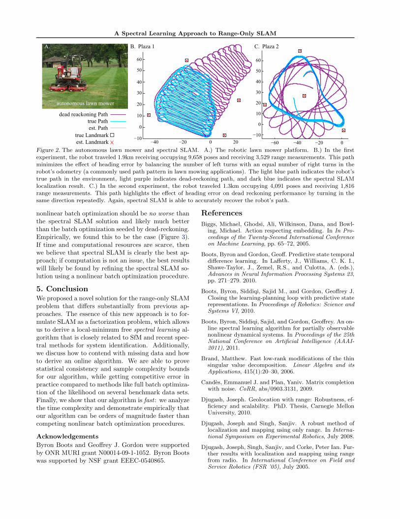
Figure 2. The autonomous lawn mower and spectral SLAM. A.) The robotic lawn mower platform. B.) In the firstexperiment, the robot traveled 1.9km receiving occupying 9,658 poses and receiving 3,529 range measurements. This pathminimizes the e↵ect of heading error by balancing the number of left turns with an equal number of right turns in therobot’s odometry (a commonly used path pattern in lawn mowing applications). The light blue path indicates the robot’strue path in the environment, light purple indicates dead-reckoning path, and dark blue indicates the spectral SLAMlocalization result. C.) In the second experiment, the robot traveled 1.3km occupying 4,091 poses and receiving 1,816range measurements. This path highlights the e↵ect of heading error on dead reckoning performance by turning in thesame direction repeatedly. Again, spectral SLAM is able to accurately recover the robot’s path.

nonlinear batch optimization should be no worse thanthe spectral SLAM solution and likely much betterthan the batch optimization seeded by dead-reckoning.Empirically, we found this to be the case (Figure 3).If time and computational resources are scarce, thenwe believe that spectral SLAM is clearly the best ap-proach; if computation is not an issue, the best resultswill likely be found by refining the spectral SLAM so-lution using a nonlinear batch optimization procedure.

5. ConclusionWe proposed a novel solution for the range-only SLAMproblem that di↵ers substantially from previous ap-proaches. The essence of this new approach is to for-mulate SLAM as a factorization problem, which allowsus to derive a local-minimum free spectral learning al-gorithm that is closely related to SfM and recent spec-tral methods for system identification. Additionally,we discuss how to contend with missing data and howto derive an online algorithm. We are able to provestatistical consistency and sample complexity boundsfor our algorithm, while getting competitive error inpractice compared to methods like full batch optimiza-tion of the likelihood on several benchmark data sets.Finally, we show that our algorithm is fast : we analyzethe time complexity and demonstrate empirically thatour algorithm can be orders of magnitude faster thancompeting nonlinear batch optimization procedures.

AcknowledgementsByron Boots and Geo↵rey J. Gordon were supportedby ONR MURI grant N00014-09-1-1052. Byron Bootswas supported by NSF grant EEEC-0540865.

References

Biggs, Michael, Ghodsi, Ali, Wilkinson, Dana, and Bowl-ing, Michael. Action respecting embedding. In In Pro-ceedings of the Twenty-Second International Conferenceon Machine Learning, pp. 65–72, 2005.

Boots, Byron and Gordon, Geo↵. Predictive state temporaldi↵erence learning. In La↵erty, J., Williams, C. K. I.,Shawe-Taylor, J., Zemel, R.S., and Culotta, A. (eds.),Advances in Neural Information Processing Systems 23,pp. 271–279. 2010.

Boots, Byron, Siddiqi, Sajid M., and Gordon, Geo↵rey J.Closing the learning-planning loop with predictive staterepresentations. In Proceedings of Robotics: Science andSystems VI, 2010.

Boots, Byron, Siddiqi, Sajid, and Gordon, Geo↵rey. An on-line spectral learning algorithm for partially observablenonlinear dynamical systems. In Proceedings of the 25thNational Conference on Artificial Intelligence (AAAI-2011), 2011.

Brand, Matthew. Fast low-rank modifications of the thinsingular value decomposition. Linear Algebra and itsApplications, 415(1):20–30, 2006.

Candes, Emmanuel J. and Plan, Yaniv. Matrix completionwith noise. CoRR, abs/0903.3131, 2009.

Djugash, Joseph. Geolocation with range: Robustness, ef-ficiency and scalability. PhD. Thesis, Carnegie MellonUniversity, 2010.

Djugash, Joseph and Singh, Sanjiv. A robust method oflocalization and mapping using only range. In Interna-tional Symposium on Experimental Robotics, July 2008.

Djugash, Joseph, Singh, Sanjiv, and Corke, Peter Ian. Fur-ther results with localization and mapping using rangefrom radio. In International Conference on Field andService Robotics (FSR ’05), July 2005.

A Spectral Learning Approach to Range-Only SLAM

Method Plaza 1 Plaza 2

Dead Reckoning (full path) 15.92m 27.28m

Cartesian EKF (last, best 10%) 0.94m 0.92mFastSLAM (last, best 10%) 0.73m 1.14mROP EKF (last, best 10%) 0.65m 0.87m

Batch Opt. (worst 10%) 1.04m 0.45mBatch Opt. (last 10%) 1.01m 0.45mBatch Opt. (best 10%) 0.56m 0.20mBatch Opt. (full path) 0.79m 0.33m

Spectral SLAM (worst 10%) 1.01m 0.51mSpectral SLAM (last 10%) 0.98m 0.51mSpectral SLAM (best 10%) 0.59m 0.22mSpectral SLAM (full path) 0.79m 0.35m

Spectral + Batch Optimization (worst 10%) 0.89m 0.40mSpectral + Batch Optimization (last 10%) 0.81m 0.32mSpectral + Batch Optimization (best 10%) 0.54m 0.18mSpectral + Batch Optimization (full path) 0.69m 0.30m Plaza 1 Plaza 2

0.73 0.51

9264.55

2357.09

Batch Opt.

Spectral SLAM

~~~~

Runtime (seconds)

Figure 3. Comparison of Range-Only SLAM Algorithms. The table shows Localization RMSE. Spectral SLAM haslocalization accuracy comparable to batch optimization on its own. The best results (boldface entries) are obtained byinitializing nonlinear batch optimization with the spectral SLAM solution. The graph compares runtime of Gauss-Newtonbatch optimization with spectral SLAM. Empirically, spectral SLAM is 3-4 orders of magnitude faster than full batchoptimization of the likelihood on the autonomous lawnmower datasets.

Ferris, Brian, Fox, Dieter, and Lawrence, Neil. WiFi-SLAM using Gaussian process latent variable models.In Proceedings of the 20th international joint conferenceon Artifical intelligence, IJCAI’07, pp. 2480–2485, SanFrancisco, CA, USA, 2007. Morgan Kaufmann Publish-ers Inc.

Hsu, Daniel, Kakade, Sham, and Zhang, Tong. A spectralalgorithm for learning hidden Markov models. In COLT,2009.

Kanade, T. and Morris, D.D. Factorization methodsfor structure from motion. Philosophical Transactionsof the Royal Society of London. Series A: Mathemati-cal, Physical and Engineering Sciences, 356(1740):1153–1173, 1998.

Kantor, George A and Singh, Sanjiv. Preliminary resultsin range-only localization and mapping. In Proceedingsof the IEEE Conference on Robotics and Automation(ICRA ’02), volume 2, pp. 1818 – 1823, May 2002.

Kehagias, Athanasios, Djugash, Joseph, and Singh, Sanjiv.Range-only SLAM with interpolated range data. Techni-cal Report CMU-RI-TR-06-26, Robotics Institute, May2006.

Kurth, Derek, Kantor, George A, and Singh, Sanjiv. Ex-perimental results in range-only localization with radio.In 2003 IEEE/RSJ International Conference on Intelli-gent Robots and Systems (IROS ’03), volume 1, pp. 974– 979, October 2003.

Montemerlo, Michael, Thrun, Sebastian, Koller, Daphne,and Wegbreit, Ben. FastSLAM: A factored solution tothe simultaneous localization and mapping problem. InIn Proceedings of the AAAI National Conference on Ar-tificial Intelligence, pp. 593–598. AAAI, 2002.

Rosencrantz, Matthew, Gordon, Geo↵rey J., and Thrun,Sebastian. Learning low dimensional predictive repre-sentations. In Proc. ICML, 2004.

Siddiqi, Sajid, Boots, Byron, and Gordon, Geo↵rey J.Reduced-rank hidden Markov models. In Proceedingsof the Thirteenth International Conference on ArtificialIntelligence and Statistics (AISTATS-2010), 2010.

Thrun, Sebastian, Burgard, Wolfram, and Fox, Di-eter. Probabilistic Robotics (Intelligent Robotics andAutonomous Agents). The MIT Press, 2005. ISBN0262201623.

Tipping, Michael E. and Bishop, Chris M. Probabilisticprincipal component analysis. Journal of the Royal Sta-tistical Society, Series B, 61:611–622, 1999.

Tomasi, Carlo and Kanade, Takeo. Shape and motionfrom image streams under orthography: a factorizationmethod. International Journal of Computer Vision, 9:137–154, 1992.

Triggs, B. Factorization methods for projective structureand motion. In Computer Vision and Pattern Recogni-tion, 1996. Proceedings CVPR’96, 1996 IEEE ComputerSociety Conference on, pp. 845–851. IEEE, 1996.

Van Overschee, P. and De Moor, B. Subspace Identificationfor Linear Systems: Theory, Implementation, Applica-tions. Kluwer, 1996.

Yairi, Takehisa. Map building without localization by di-mensionality reduction techniques. In Proceedings ofthe 24th international conference on Machine learning,ICML ’07, pp. 1071–1078, New York, NY, USA, 2007.ACM.