A Spectral Index for Land Degradation Mapping Using ASTER Data Application to a Semi-Arid...

www.elsevier.com/locate/jag

International Journal of Applied Earth Observation

and Geoinformation 7 (2005) 140–153

A spectral index for land degradation mapping using ASTER data:

Application to a semi-arid Mediterranean catchment

Mohamed Chikhaoui a,*, Ferdinand Bonn a,Amadou Idrissa Bokoye a, Abdelaziz Merzouk b

a CARTEL (Centre d’Applications et de Recherches en Teledetection), Universite de Sherbrooke,

2500 boul. de l’Universite. Sherbrooke, Que., Canada J1K 2R1b Departement Science du Sol – IAV Hassan I, B.P. 6002, Rabat Institut, Rabat, Morocco

Received 28 November 2003; accepted 23 January 2005

Abstract

Flagrant soil erosion in Morocco is an alarming sign of soil degradation. Due to the considerable costs of detailed ground

surveys of this phenomenon, remote sensing is an appropriate alternative for analyzing and evaluating the risks of the expansion

of soil degradation. In this paper, we characterize the state of land degradation in a small Mediterranean watershed using

Advanced Spaceborne Thermal Emission and Reflection Radiometer (ASTER) data and ground-based spectroradiometric

measurements. The two visible, the near-infrared and six shortwave infrared bands of the above sensor were calibrated using

ground measurements of the spectral reflectance. Field measurements were carried out in the Saboun experimental basin located

in the marl soil region of the Moroccan western Rif. The study leads to the development and evaluation of a new spectral

approach to express land degradation. This index called Land degradation index (LDI) is based on the concept of the soil line

derived from spectroradiometric ground measurements. In this study, we compare LDI and the spectral angle mapping (SAM)

approaches to assess and map land degradation. Results show that LDI provides more accurate results for mapping land

degradation (Kappa = 0.79) when compared to the SAM method (Kappa = 0.61). Validation and evaluation of the results are

based on the thematic maps derived from the ground data (organic matter, clay, silt and sand) by kriging, DEM, slope gradient

and photointerpretation.

# 2005 Elsevier B.V. All rights reserved.

Keywords: Land degradation; Land degradation index (LDI); ASTER; Spectral angle mapping (SAM); ASD and spectroradiometry;

Morocco; Erosion

* Corresponding author. Tel.: +1 819 821 8000/2945;

fax: +1 819 821 7944.

E-mail address: [email protected] (M. Chikhaoui).

0303-2434/$ – see front matter # 2005 Elsevier B.V. All rights reserved

doi:10.1016/j.jag.2005.01.002

1. Introduction

Land degradation, defined as the loss or the

reduction of the potential utility or productivity of

the land (Lal, 1994), is a major environmental problem

in arid and semi-arid areas. In the north of Morocco,

.

M. Chikhaoui et al. / International Journal of Applied Earth Observation and Geoinformation 7 (2005) 140–153 141

land degradation is mainly caused by soil erosion,

ecosystem changes, landslides, deforestation and

human pressure through over-cultivation and mechan-

isation. Soil erosion, with annual soil losses varying

between 2000 and 6000 t/km2/year (MAMVA, 1993),

is a major environmental and economic problem that

threatens the sustainability of dam reservoirs and

agricultural lands in the Rif Mountains. Despite its

importance, the measurement of the spatial extent of

this phenomenon by conventional methods (USLE,

MUSLE and RUSLE) is not usually accurate (Bonn et

Escadafal, 1996; Bonn, 1998).

The land degradation process is generally divided

into three classes: (1) physical degradation, (2)

biological degradation, and (3) chemical degradation

(Barrow, 1991). The assessment of land degradation

requires the identification of indicators such as soil

vulnerability to erosion. Generally, the assessment of

the state of land degradation can be carried out using

the Global Assessment of Soil Deterioration (GLA-

SOD) method (Oldeman et al., 1991). Hoosbeek et al.

(1997) recommended this qualitative method to

classify soil degradation using remote sensing data.

Degradation features can be detected directly or

indirectly by using image data. Previous studies

proposed spectral unmixing using a linear model to

study soil degradation (Hill et al., 1995; Van der

Meer, 1997; Metternicht and Fermont, 1998;

Haboudane, 1999). The analyses of the fraction

images yield the most information about soil

degradation (Hill et al., 1995). Other authors have

established a relationship between the vegetation

cover fraction and erodibility (Hudson, 1957, 1971;

Roose et al., 1993). The vegetation cover fraction can

be estimated approximately from remote sensing

images through vegetation indices (Cyr et al., 1995;

Biard and Baret, 1997; Hill et al., 1998; Arsenault

and Bonn, 2001). However, the relationships between

actual vegetation cover and the vegetation indices are

not easily applicable to all land cover types. Previous

research have proposed a color index, form index and

intensity index for mapping land degradation

(Escadafal et al., 1994; Mougenot and Cailleau,

1995; Escadafal and Bacha, 1995; Haboudane et al.,

2002). These indices were developed based on past

generation remote sensing sensors. However, the use

of data from new generation space remote sensing

sensors like advanced spaceborne thermal emission

and reflection radiometer (ASTER) requires that

these indices be adapted.

The principal objective of this study is thus to

develop and evaluate a new spectral index for the study

of land degradation using ASTER by exploiting the

potential of its three VNIR (visible-near infrared) and

six SWIR (short wave infrared) bands. The potential

of ASTER data for mapping land degradation through

the application of this new proposed spectral index and

the spectral angle mapping (SAM) (Kruse et al., 1993)

approaches to a semi-arid area of northern Morocco is

also investigated. Comparison of the results obtained

by the two approaches should allow the evaluation of

the most appropriate one for land degradation

mapping.

Data collection is described in the next section.

Section 3 exposes the remote sensing methods

considered for land degradation mapping. Results

and the validation of retrieved soil degradation maps

are reported in Section 4. A general conclusion is

outlined in Section 5.

2. Study area and data acquisition

2.1. Study area

The study was carried out in the Saboun (720 ha)

experimental catchment located in the western Rif of

Morocco (Fig. 1) for which soil, hydrological and

erosion databases are available. The Saboun

watershed is composed mainly of the Tangiers

geological unit. It is characterized by predominantly

altered argillaceous, gray and yellow shale facies

dating from the Senonian. The soils of the basin have a

predominance of swelling clays (montmorillonite and

smectite). Oligo-Miocene deposits with shaley facies

and Quaternary deposits can also be found (Thauvin,

1971).

The soil map (Fig. 2) covering the study area was

established by the Direction provinciale de l’agri-

culture de Tetouan (INRA, 1983) and shows the

presence of four soil classes: vertisols (Typic

Chromoxerert), paravertisols (Vertic Palexeroll), cal-

cimagnesic (Typic Calcixeroll) and poorly developed

(Vertic Xerothent).

The Saboun watershed is subject to intensive

agricultural activity. The climate in the region is

M. Chikhaoui et al. / International Journal of Applied Earth Observation and Geoinformation 7 (2005) 140–153142

Fig. 1. Study area: the Saboun basin in Morocco.

Mediterranean. mean annual rainfall amounts to

743 mm with an interannual coefficient of variation

of 23% (Chikhaoui, 1998). Temperatures vary

between 7 8C (monthly minimum average) and

26 8C (monthly maximum average).

The Saboun basin presents interesting character-

istics for our study with regards to the erosion

phenomena. It has the same lithology and it faces the

same soil degradation problem as most of the western

Rif region. This allows for a regional generalization of

the results. The lithological variability observed

within the watershed constitutes a unit that permits

the evaluation and validation of our approach. Based

Fig. 2. Soil map of the Saboun basin.

on field observations, three soils degradation classes

were identified in our basin (Fig. 3):

- S
lightly degraded soils: part of the surface soil is
removed and affected by overland and sheet runoff.

This class is occupied by olive orchards and

agricultural land is cultivated with cereals.

- M
oderately degraded soils: large part of topsoil is
removed and also affected by rills, overland and

sheet runoff with sparse vegetation. This class is

dominated by pasture land.

- H
ighly degraded soils: all topsoil and part of
subsoil or substratum is removed. The surface is

affected by rills, gullies and bank undermining

forms of erosion. We noted a physical deterioration

caused by domestic animals (compaction). This

class is characterized by steep hillsides and mostly

ploughting in the slope direction.

2.2. Field spectroradiometric data

The spectroradiometer used on the ground is a high

spectral resolution analytical spectral device (ASD). It

operates in the visible, the near infrared and the

shortwave infrared (350–2500 nm). The radiometric

measurements were carried out with resolution

intervals of 10 nm between 350 and 1000 nm and

20 nm between 1000 and 2500 nm. The apparatus is

installed on a tripod at a height varying between 1.50

and 2 m from the ground. This position permits the

vertical viewing of a circular surface with a radius of

approximately 25 cm. A Spectralon board served as

reference before and after each measurement. This

permits the calculation of the target reflectance factor

according to the method described by Jackson et al.

(1980). The objective of this procedure is to minimize

errors due to variations in atmospheric conditions and

sun inclination. The bidirectional effects of the target

reflectance were accounted for by carrying out

measurements over very short and close time intervals

and by keeping the viewing angle constant and in a

vertical position.

The measurement campaign was conducted

between 18 and 26 October 2000. The choice of the

measurement sites is based on the soil, geological and

topographic maps and our knowledge of the study area

so as include most of the surface conditions or the

different levels of soil degradation. The present study


Fig. 3. Soil degradation classes identified in our basin. (A) Highly degraded soils, (B) moderately degraded soils, and (C) slightly degraded soils.

focuses on the characterization of the state of soil

surface conditions and land degradation by water

erosion Wt (Loss of topsoil) and Wd (Terrain

deformation/mass movement) according to the global

assessment of soil deterioration (GLASOD) method

(Oldeman et al., 1991). Three classes of soil

degradation identified in Section 2.1 are found which

correspond to classes 1–3 of GLASOD.

The characterization of the spectral properties of

the different soil types was carried out based on the

technique of principal components analysis (PCA)

using the ground spectra (Chikhaoui et al., 2001). A K-

means analysis was subsequently applied. This

permitted the discrimination of the different classes

corresponding to the level of degradation. To obtain

these results, the relative coordinates at the orthogonal

level (PC1 and PC2) of the 20 spectra were adopted.

This method is detailed in Leone and Sommer (2000)

and Chikhaoui et al. (2001). Simulation of the ASTER

bands was carried out by convolution of the values of

the spectral responses of the ASTER bands with

reflectance curves of samples under investigation.

This process was computed using the ENVI software

(ENVI, 2001).

Table 1

ASTER sensor characteristics

VNIR (mm) S

Bands

B

B1: 0.520–0.600 (Nadir) B

B2: 0.630–0.690 (Nadir) B

B3N: 0.760–0.860 (Nadir) B

B3B: 0.760–0.860 (� inclined by 248) B

B

Spatial resolution (m)

15 3

2.3. ASTER data and preprocessing

ASTER is a multiband imaging radiometer

installed on the Terra platform in 1999. It is the

result of a collaborative effort between NASA and

the Japanese Ministry of Economy Trading and

Industry (METI), formerly known as the Ministry of

International Trade and Industry (MITI). The

ASTER sensor is equipped with a stereoscopic

acquisition mode permitting the extraction of digital

terrain models. It has 14 bands with a spectral

resolution varying from 0.52 to 11.65 mm. The

sensor itself is equipped with three separate radio-

meters (Abrams, 1997). They cover respectively the

three following portions of the spectral domain: the

visible and the near infrared (NIR), the shortwave

infrared (SWIR) and the thermal (Table 1). This

study covers only VNIR and SWIR spectral bands,

and the TIR spectral bands of ASTER were not

used.

The ASTER sensor is characterized by a repeat

cycle of 16 days and provides a scene of the order of

60 km � 60 km. It follows the same orbit as Landsat 7

but 30 min later.

WIR (mm) TIR (mm)

4: 1.600–1.700

5: 2.145–2.185 B10: 8.125–8.475

6: 2.185–2.225 B11: 8.475–8.825

7: 2.235–2.285 B12: 8.925–9.275

8: 2.295–2.365 B13: 10.250–10.950

9: 2.360–2.430 B14: 10.950–11.650

0 90


ig. 4. Spectral angle between the reference spectrum and the

The ASTER scene used for the study was acquired

during the month of June 2001. It corresponds to level 2:

AST_07, which contains the surface reflectance. The

image was corrected atmospherically and radiometri-

cally by the image provider. The geometric correction

was carried out using a polynomial approach. We

applied a correction to the image in relation to the

1:50,000 topographic map covering the study area. The

transfer equation is a first degree polynomial function

calculated from the control points. Resampling was

carried out using the nearest neighbor method so as not

to severely alter the pixel values. Using the least squares

method, the correction accuracy was determined by

calculating the residual errors between the value

obtained by the application of the function and the

true value. The corrected bands were then resampled to

the same spatial resolution to obtain the same pixel size

(15 m). Following these steps, the ASTER data were

orthorectified using the digital elevation model (DEM).

Previous work (Rowan and Mars, 2003; Iwasaki

et al., 2001) underlined a significant difference

between the measurements acquired on the ground

and the ASTER (AST_07) image data. Band 9 has a

higher reflectance value of the order of 10–20% than

the value measured on the ground and the same occurs

with band 3. This difference can be explained by a

crosstalk instrument problem (Iwasaki et al., 2001).

This phenomenon is caused by light reflected from the

band 4 optical components leaking into other SWIR

band detectors particularly band 9.

To compensate for this problem, we calibrated the

image data by adopting the method of spectral

matching (Rowan and Mars, 2003). This consists in

a comparison of the image data with the simulated

ASTER data using the spectral measurements

acquired over the same site. We chose as target an

agricultural plot with bare soil which is characterized

by a slope almost equal to zero.

The image was calibrated by multiplying it by a

calculated normalizing factor Fn (Eq. (1)). The

simulated value and the one extracted from the image

must be of the same site.

Fn ¼ value of the simulated band

average value of target area taken from the image

(1)

3. Land degradation mapping methods

Several methods were developed to map land

features from spatial remote sensing data. Here, we

consider the widely used spectral angle mapping

method and a new approach developed through the

present work (see Section 1).

3.1. Spectral angle mapper (SAM)

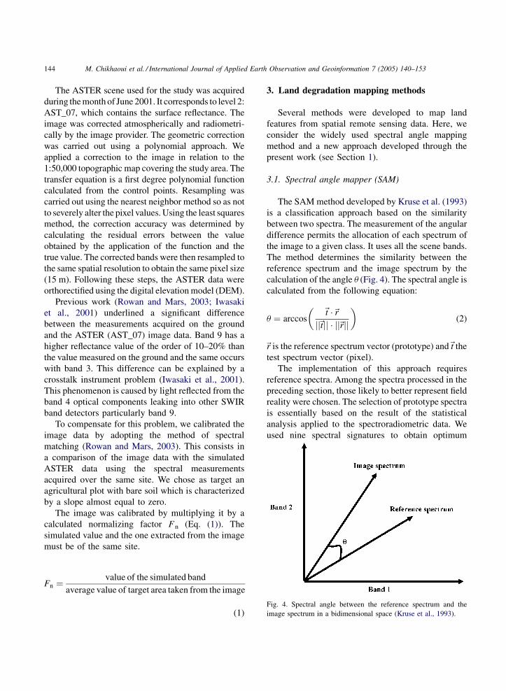
The SAM method developed by Kruse et al. (1993)

is a classification approach based on the similarity

between two spectra. The measurement of the angular

difference permits the allocation of each spectrum of

the image to a given class. It uses all the scene bands.

The method determines the similarity between the

reference spectrum and the image spectrum by the

calculation of the angle u (Fig. 4). The spectral angle is

calculated from the following equation:

u ¼ arccos

�~t �~r

jj~tjj � jj~rjj

�(2)

~r is the reference spectrum vector (prototype) and~t the

test spectrum vector (pixel).

The implementation of this approach requires

reference spectra. Among the spectra processed in the

preceding section, those likely to better represent field

reality were chosen. The selection of prototype spectra

is essentially based on the result of the statistical

analysis applied to the spectroradiometric data. We

used nine spectral signatures to obtain optimum

age spectrum in a bidimensional space (Kruse et al., 1993).

F

im


ground modeling. We did our upmost to respect a

composition containing three spectral signatures

representing each stage of soil degradation.

The approach considers the pixel values as a

vector in a space with a size equal to the number of

bands. The method is rigorous and not sensitive to

albedo if one uses calibrated data. The attribution of

each scene pixel to a given class by the SAM

approach is based on the measurement of the angle

between the reference spectrum vector and each

image vector in the n-dimension space (Fig. 4) where

n is the number of bands. The implementation of the

SAM approach gives an image with an angle u for

each reference spectrum. Using the u angle images,

we carried out a thresholding to attribute the theme

that has the lowest u value to each pixel; the smaller

the angular difference, the higher is the similarity.

The selection of this approach in the present study is

justified by the fact that Margate and Shrestha (2001)

adopted the SAM approach for the study of soil

degradation and desertification in southern Spain

and obtained satisfactory results. Also, the adoption

of SAM in other similar studies has provided

satisfactory results (Sohn et al., 1999; Sohn

and Rebello, 2002; Yang et al., 1999; Zhang et al.,

2003). SAM is a method designed for a spectral

space of n-dimensions and available in the ENVI

image analysis software. The current application of

the SAM method remains original compared to the

above cases. In fact, ASTER data are used for the

first time with this method for mapping land

degradation.

Fig. 5. Concept of the LDI approa

3.2. A new approach: LDI

This approach is based on the soil line concept and

its use requires ground based data. The implementa-

tion of this method relies both on a slightly degraded

bare soil line and a highly degraded bare soil line. The

definition of these lines requires a collection of points

from the pixels of the image itself or derived from

ground spectral measurements. The use of ground

data necessitates the calibration of the image data in

order to produce a reflectance image corrected for

atmospheric and instrumental effects. The principle

behind our approach is simple. It is inspired by the

SAM classification approach and the CRIM index

(Crop Residue Index Multiband) (Biard and Baret,

1997). In a bidimensional space defined by two

spectral bands, any point P representing bare soil is

located between the highly degraded bare soil line and

that of the slightly degraded soil line (Fig. 5). The

calculation of the highly and slightly degraded soil

line is carried out after the classification and

processing of the spectroradiometric data. Our

method, which does not limit itself to the choice of

specific bands, is called the land degradation index

(LDI).

The ratio between the distance P over the highly

degraded soil line (DP) and the distance between the

highly and slightly degraded soil lines (DE) allows the

attribution of any point to a given class. The

calculation of the tangent of angles a and b (Fig. 5)

measures the distance DE and DP. Point I corresponds

to the interception point of the two lines. The LDI can

ch in a bidimensional space.


Fig. 6. Soil sampling points in the basin.

be estimated in a bidimensional space by the following

equation:

LDI ¼ tan a

tan b¼ cos b

cosa�

ffiffiffiffiffiffiffiffiffiffiffiffiffiffiffiffiffiffiffiffiffi1 � cos2 a

1 � cos2 b

s(3)

It can also be estimated in the following form:

LDI ¼ DP

DE¼ tan a

tan b(4)

LDI can be adapted to an n-dimension space, knowing

that n is the number of bands. In this case, the highly

degraded soil line and that of the slightly degraded

soils can be defined by using many spectral bands and

by selecting a single band as reference. In the present

study, it is useless to repeat the demonstration for

calculating the cosine of an angle defined by two lines

in an n-dimension space; this passage is largely devel-

oped by Biard and Baret (1997).

3.3. Validation procedure

The stereoscopic analysis serves to define and

delimit the geomorphologic indicator such as erosion

forms over the basin area. The results will be

integrated into a GIS for the validation of results

obtained from the satellite image processing. The

aerial photographs used in this study were acquired on

June 1996 at the scale of 1/20,000. The results derived

from the laboratory physico-chemical analysis of the

samples acquired on the ground focused on the content

in total calcium, organic matter and grain size.

Following that, the analysis of the spatial variability of

these data was carried out using geostatistical

processing provided by the GS+ (Robertson, 1998)

software. In this study, kriging was adopted as

interpolation method because it is a non-biased linear

method. After, we obtained thematic maps for each

variable measured. To reach our objective, we carried

out a systematic sampling following a standard grid

with 350 m � 350 m spacing. Each soil sample was

acquired at the soil surface at a depth of 5–10 cm;

Fig. 6 shows the location of the 60 sampling points.

Factors responsible for spatial differences in land

degradation such as slope gradient, lithology and soil

proprieties were used to analyze the distribution of

land degradation classes in relation to these factors.

The DEM was generated using the topographic map

(1/50,000) with the Arc View software. Slope gradient

was computed from the DEM.

The thematic maps were resampled to the same

pixel size (15 m). A total of 120 points selected

randomly over the surface conditions map were used

with the thematic map to determine the accuracy

assessment. The error matrix served to calculate the

global accuracy and KHAT statistic (an estimate of the

kappa coefficient) (i.e., K). KHAT statistic is another

measure of accuracy. It was calculated by Congalton

(1991) as

K ¼ NPr

i¼1 xii �Pr

i¼1ðxiþ � xþiÞN2 �

Pri¼1ðxiþ � xþiÞ

(5)

where r is the number of rows in the matrix, xii the

number of observations in row i and column i, xi+

and x+i are the marginal totals of row i and column i,

respectively, and N is the total number of observa-

tions.

The efficiency and accuracy of the two approaches

were evaluated using KHAT statistic K and its

variance (i.e., s2) as follows:

s2ðKÞ ¼ 1

N

a1ð1 � a1Þð1 � a2Þ2

þ 2ð1 � a1Þð2a1a2 � v1Þð1 � a2Þ3

þ ð1 � a1Þ2ðv2 � 4a22Þ

ð1 � a2Þ4(6)


where

v1 ¼Xr

i¼1

xiiðxiþxþiÞ; v2 ¼Xr

i¼1

Xr

i¼1

xi jðxþ jx jþÞ;

a1 ¼Xr

i¼1

xii; a2 ¼Xr

i¼1

xiþxþi; xi j ¼xiþxþi

N:

To test the significance of the differences between the

two approaches, the method described by Cohen

(1960) is used. The method uses the normal curve

deviate statistics Z given by

Z ¼ K1 � K2ffiffiffiffiffiffiffiffiffiffiffiffiffiffiffiffis2

1 þ s22

q (7)

4. Results

4.1. Analysis and classification of the

spectroradiometric data

Fig. 7 shows the soil spectra collected over the

Saboun basin. The bare soil spectra are characterized by

a progressive increase in reflectance as the wavelength

increases (Fig. 7). Slightly degraded soils can be

distinguished by low reflectance with a pronounced

absorption band corresponding to clays at 2.20 mm.

Highly degraded soil spectra are characterized by

relatively high reflectance with a higher spectral slope

between VIS-NIR than for slightly degraded soils. The

highly degraded soil spectra are characterized by

spectral absorption around 2.35 mm due to carbonates.

Fig. 7. Soil spectra from the Saboun watershed. Slightly degraded soils in g

green.

In other words, changes in soil surface conditions

modify the shape of the soil reflectance spectra.

Multivariate statistical analysis of these spectral data

enabled us to better discriminate between the different

levels of soil degradation (Chikhaoui et al., 2001).

Subsequently, we retained two data groups. One

represents slightly degraded soils and the second

represents highly degraded soils.

In a bidimensional scatter plot, Fig. 8 shows that the

soil-line concept is valid between any couple of the

ASTER spectral bands for all soils of every data

group. This concept is verified for both groups of soil

surface conditions. This confirms the result obtained

by Baret et al. (1993). Band 2 as reference provided a

better result for the different combinations (Fig. 8).

4.2. Accuracy assessment

4.2.1. Land degradation mapping using the SAM

approach

The selection of prototype spectra is based

essentially on the results of the statistical analysis

applied to the spectroradiometric data. A u angle

image is produced for each reference spectral

signature. From these images, we produced first a

thematic map of the soils by attributing to each pixel

the theme having a low u value. The value of 0.20 rad

is defined as a threshold value for the maximum angle

between the image vector and the reference vector

spectrum. With this value, it is possible to obtain many

different thematic classes. Secondly, we studied the

state of soil degradation using the spectral signatures

associated with the different levels of soil degradation.

The regrouping of the thematic classes into one single

reen, moderately degraded soils in blue and highly degraded soils in


Fig. 8. (1) Highly degraded bare soil line. (2) Slightly degraded bare soil line.

class expressing the state of soil degradation according

to the spectroradiometric data classification provided

the basis for the thematic map presented in Fig. 9.

Classification accuracy results from the SAM method

are shown in Table 2 with an overall accuracy of 0.73

and includes the error matrix. According to this data,

the highly degraded soils were mapped with high

producer’s accuracy (omission error) (>0.87).

The analysis of the results of the SAM approach

shows that the moderately degraded soils dominate

with 41%. The value of 0.20 rad made it possible to

obtain satisfactory classification results and variations

of this value generate significant changes in the

classification results. Values above this threshold

produced a large number of nonclassified pixels and

less thematic classes. The water class (dam reservoir)

is identified as unclassified pixels by the SAM method.

Fig. 9. Soil surface conditions map obtained with the SAM

approach.

This result can be explained by the absence of spectral

signatures representing this class.

4.2.2. Land degradation mapping using the LDI

approach

ASTER Band 2 (0.63–0.69 mm) was used as

reference band and provided satisfactory results.

The choice of this band is based on the principle

that for any spectral band combination, the concept of

the soil line is verified and that pixels should be

located between the two lines in a multidimensional

spectral space. In other words, the LDI index should

have a value between 0 and 1 (Fig. 10.1). The

implementation of the LDI algorithm uses all the

bands of the spectral domain in the visible, NIR and

SWIR.

Fig. 10.1 shows the results obtained with the LDI

index. We observe that the highly degraded soils have

a high LDI index value with 0.60 and we note that the

slightly degraded soils have a quite small LDI value

with 0.20. The application of a thresholding to the

able 2

ccuracy assessment result of the SAM classification method

lass Producer’s

accuracy

User’s

accuracy

lightly degraded soils 0.65 0.70

oderately degraded soils 0.68 0.76

ighly degraded soils 0.87 0.74

verall accuracy 0.73

HAT statistic and variance K ¼ 0:61 and

s2 = 0.0024

T

A

C

S

M

H

O

K


Fig. 10. Surface conditions map determined by the LDI.

histogram of the LDI index provided well defined

classes. Subsequently, we applied a median filter with

a 3 � 3 window to obtain homogeneous classes and to

reduce the presence of isolated pixels. Fig. 10.2 shows

the results of this post-processing. Classification

accuracy results for the LDI approach are shown in

Table 3. The LDI method seems to provide more

accurate results for mapping land degradation when

compared to the SAM method with an overall

accuracy of 0.85. According to the error matrix, the

highly degraded soils were mapped with high user’s

(commission error) and producer’s accuracy (>0.92).

Moreover, we observe that the pixels of the dam

reservoir have small values between 0.20 and 0.35.

These values can be explained by the low water level

behind the dam. The dam is characterized by a

Table 3

Accuracy assessment result of the LDI approach

Class Producer’s

accuracy

User’s

accuracy

Slightly degraded soils 0.83 0.79

Moderately degraded soils 0.83 0.85

Highly degraded soils 0.92 0.95

Overall accuracy 0.85

KHAT statistic and variance K ¼ 0:79 and

s2 = 0.0015

relatively high rate of silting reaching 2% of its storage

capacity per year according to the last bathymetric

campaign (UR AMBRE, 2002). It represents a

sedimentation site for the fertile elements of the lands

upstream which were transported by water. Moreover,

we can observe that the thematic map produced by the

application of the LDI index shows a dominance of

poorly developed soils of the order of 39%.

4.3. Validation and discussion of results

Comparison of the results obtained by the two

approaches reveals that LDI produced a much higher

accuracy than SAM with KHAT statistic = 0.79.

According to Montserud and Leamans (1992) this

value indicates that the method shows very good to

excellent classification performance. We observe that

the results obtained with the two approaches are

similar overall and clearly show the degraded soil

class. This can be explained by the fact that the

spectral response of these soils types is invariant. In

fact, we can observe a strong contribution from the

substratum in the spectral signature of this soil class.

In other words, this can be explained by the large areas

of bare soil and the high reflectance of the ground

substrate. Moreover, we note that the SAM method has

a tendency sometimes to agglomerate the slightly and


the moderately degraded soils into one single class.

This is due to the fact that, on the one hand, the SAM

approach is based on the spectral similarity approach

(Crosta et al., 1998) and, on the other hand, it must be

stressed that the adoption of only one angular

threshold (0.20 rad) for the different classes some-

times introduces this confusion. The latter can be

explained by the heterogeneity of the surface state:

roughness, moisture and the presence of some crop

residues. Also, it must be noted that the acquisition of

the ground spectroradiometric data and the image data

was not carried out simultaneously. Since the image

and radiometric spectra were not acquired during the

same year and because of the small time difference

between the acquisition dates (summer for the image

and fall for the spectra), it is self-evident that this

could induce a certain confusion when using the SAM

method. This is the case for the soil cover rate and

roughness. The seasonal difference is accompanied by

a variation in the ground cover rate (higher in summer

than in the fall: presence of thatch), and this also has an

effect on the results. Also, the fall season during which

the spectra were collected on the ground corresponds

to the tilling period. Our approach based on the use of

LDI enabled us to get more detailed quantitative

results for every pixel. In addition, it helped in limiting

the confusion that exists in the SAM method. As such,

it is very sensitive to the u angle and produced no

satisfactory results because with values above this we

obtained a thematic map with one or two classes or a

large number of non-classified pixels.

Tables 2 and 3 show the KHAT statistic used for the

accuracy evaluation. The difference between the two

approaches shows the interest and the contribution of

LDI in the study of land degradation. We found that Z

is 2.88. This value exceeds Zt = 1.96 with a 95%

confidence level, and hence the difference between the

LDI and SAM methods is significant, and shows the

interest and the contribution of the LDI index in the

study of land degradation. However, it must be noted

that although the LDI index remains sensitive to the

Table 4

Severity of the land degradation in our area study

Severity Erosion form Symbol E

Slight Overland flow Sheet Wt <

Moderate Overland flow - Rills Wt

High Rills–gullies–bank undermining Wd >

vegetation cover rate, it is interesting for applications

in arid to semi-arid environments where soils are

nearly void of any vegetation cover outside the

growing season. The main cause of this limitation is

the abundance of vegetation because more than 50%

of the soil signal is masked (Bannari et al., 1996).

The use of the photo-interpretation results, DEM,

slope gradient and the thematic maps (organic matter,

clay, silt, sand) derived from the interpolation by

kriging served as an additional tool for the validation

of our results.

The analysis of the photo-interpretation result

shows that our study area is entirely affected by water

erosion. The following erosion forms were found:

overland flow, gullies, rills, and bank undermining

(Table 4). Overlay of the map of surface conditions

with the soil map, DEM and slope gradient showed that

highly degraded soils are associated with the Typic

Calcixeroll soil class. It is characterized by a soil

erodibility factor k = 0.44 measured in the laboratory

(Chikhaoui, 1998) indicating a high susceptibility to

erosion (Manrique, 1988). An examination of Table 4

shows good correlation between higher elevation, slope

gradient and the highly degraded soil class.

Also, the validation of the results obtained with the

LDI index was carried out by using a total of 20 points

located by global positioning system (GPS) in the field.

Each point had a descriptive record and a physico-

chemical analysis of one soil sample (Table 5). The

analysis of this table shows that the result derived from

the LDI approach is better than with SAM. It appears

that the map of surface conditions also depends on the

physico-chemical characteristics of the different

classes. It can clearly be seen that the slightly degraded

soil class is characterized by a low percentage of

limestone, silt and slightly more organic matter. The

highly degraded soil class is characterized by a high

percentage of silt and relatively high pH. Based on these

results, the LDI appears interesting for evaluating soil

surface conditions and opens new perspectives for

future studies in similar landscapes.

rodibility factor k Elevation (m) Slope gradient (%)

0.3 20–40 Flat (<5)

0.3 < K <0.4 50–80 10–20

0.44 80–120 >25


Tab

le5

Des

crip

tive

stat

isti

csof

the

physi

co-c

hem

ical

char

acte

rist

ics

of

the

dif

fere

nt

clas

ses

San

d(%

)C

lay

(%)

Sil

t(%

)C

aCO

3(%

)p

HC

EC

OM

(%)

Mea

nS

.E.

CV

%M

ean

S.E

.C

V%

Mea

nS

.E.

CV

%M

ean

S.E

.C

V%

Mea

nS

.E.

CV

%M

ean

S.E

.C

V%

Mea

nS

.E.

CV

%

Sli

gh

tly

deg

rad

edso

ils

24

.52

5.4

72

2.3

04

3.9

22

.41

5.4

94

5.0

74

.74

10

.52

10

.86

2.6

22

4.1

57

.80

0.1

72

.17

28

.70

10

.30

35

.88

1.8

40

.28

15

.17

Mo

der

atel

yd

egra

ded

soil

s1

7.6

74

.05

22

.92

38

.93

5.5

31

4.2

14

9.7

02

.36

4.7

61

2.6

26

.78

53

.70

8.1

50

.19

2.3

33

2.0

41

1.3

03

5.6

21

.68

0.3

11

8.8

9

Hig

hly

deg

rad

edso

ils

13

.12

4.1

73

1.7

83

5.5

82

.51

7.0

54

9.6

14

.91

9.9

11

7.7

37

.17

40

.43

8.1

30

.18

2.1

83

2.9

61

2.3

43

7.4

31

.45

0.3

52

4.1

8

OM

:org

anic

mat

ter;

CE

C:ca

tion

exch

ange

capac

ity;S

.E.:

stan

dar

der

ror;

CV

:co

effi

cien

tof

var

iati

on.T

he

num

ber

of

poin

tsuse

dfo

rth

isst

atis

tica

lpro

cess

ing

is120

(OM

,san

d,c

lay,

silt

)an

d2

0(C

aCO

3,

pH

,C

EC

).

5. Conclusion

Land degradation is a major environmental

problem in the Mediterranean area. The present study

has provided the opportunity for studying and

characterizing the state of soil degradation using a

new index called the LDI. It was able to recognize

three out of the four GLASOD land degradation

classes. ASTER data and field spectroradiometric

measurements were used for this purpose. Our results

show that both the SAM and LDI approaches have the

ability to map land degradation, although the result

provided by the LDI is more accurate with KHAT

statistic = 0.79 and that the difference between the two

methods is significant. The validation and evaluation

of the LDI are based on ground data and photo-

interpretation. Globally, the results represent ground

reality with sufficient accuracy to help the decision

makers in their soil conservation planning process.

The LDI algorithm is conceptually and methodo-

logically simple and is a useful tool for land

degradation mapping using remotely sensed data.

The advent of new superspectral and hyperspectral

sensors will allow even more extensive applications of

this spectral approach. Extrapolation of this approach

to other regions is feasible if there is a contrast

between slightly and highly degraded soils. Moreover,

the extension of the LDI approach is possible by

integrating other data sources such as geomorpholo-

gical indices (Hengl and Rossiter, 2003; Haboudane

et al., 2002). Research is currently in progress to

validate and evaluate the approach with other types of

sensors such as Landsat 7 ETM+.

Acknowledgments

We would like to thank NATO, the Canada

Research Chair on Earth Observation (Universite de

Sherbrooke), as well as the Natural Sciences and

Engineering Research Council of Canada (Grant

#OGP 6043 awarded to Dr. Bonn) for their multi-

faceted financial support during the different phases of

this study. We would also like to thank P. Cliche,

engineer at CARTEL for his technical support during

the field campaigns as well as P. Gagnon for his

linguistic support. We also thank the journal reviewers


for valuable suggestions and criticisms on the earlier

version of this manuscript.

References

Abrams, M., 1997. The advanced spaceborne thermal emission and

reflection radiometer ASTER: data products for the high spatial

resolution imager on NASA’s Terra platform. Int. J. Rem. Sens.

21, 847–859.

Arsenault, E., Bonn, F., 2001. Evaluation of soil erosion protective

cover by crop residues using vegetation indices and spectral

mixture analysis of multispectral and hyperspectral data. In:

Proceedings of the 23rd Canadian Symposium on Remote

Sensing, Sainte-Foy, Quebec-Canada, 21–24 August 2001..

Bannari, A., Huete, A.R., Morin, D., et Zagolski, F., 1996. Effets de

la couleur et de la brillance du sol sur les indices de vegetation.

Int. J. Rem. Sens. 17, 1885–1906.

Baret, F., Jacquemoud, S., Hanocq, J.F., 1993. The soil line concept

in remote sensing. Rem. Sens. Rev. 7, 62–65.

Barrow, C.J., 1991. Land Degradation: Development and Break-

down of Terrestrial Environments. Cambridge University Press,

295 p.

Biard, F., Baret, F., 1997. Crop residue estimation using multiband

reflectance. Rem. Sens. Environ. 59, 530–536.

Bonn, F. et Escadafal, R., 1996. La teledetection appliquee aux sols.

In: Bonn F. (Ed.), Chapitre 3 Precis de teledetection, vol. 2

(Applications), PUQ/AUPELF.

Bonn, F., 1998. La spatialisation des modeles d’erosion des sols a

l’aide de la teledetection et des SIG: possibilites, erreurs et

limites. Secheresse 9, 185–192.

Chikhaoui, M., 1998. Fonctionnement hydrologique et risques

d’envasement du barrage Saboun. Memoire de troisieme cycle

agronomie. IAV Hassan II, Rabat.

Chikhaoui, M., Bonn, F., Merzouk, A., Mejjati, M., et Cliche, P.,

2001. Diagnostic de l’etat de degradation du sol a partir de

l’analyse statistique des donnees spectrales: cas d’un petit bassin

du Rif marocain. In: Symposium International - Faculte des

Sciences, Marrakech, 12–15 November 2001..

Cohen, J., 1960. A coefficient of agreement for nominal scales. Edu.

Psychol. Meas. 20 (1), 37–46.

Congalton, R.G., 1991. A review assessing the accuracy of classifica-

tions of remotely sensed data. Rem. Sens. Environ. 37, 35–46.

Crosta, A.P., Sabine, C., Taranik, J.V., 1998. Hydrothermal altera-

tion mapping at Bodie, California, using AVIRIS hyperspectral

data. Rem. Sens. Environ. 65, 309–319.

Cyr, L., Bonn, F., Pesant, A., 1995. Vegetation indices derived from

remote sensing for an estimation of soil protection against water

erosion. Ecol. Model. 79, 277–285.

ENVI 3.5, User’s Guide. 2001. Research Systems Inc., Boulder, Co.,

948 p., http://www.RSInc.com.

Escadafal, R., Belghith, A., et Ben Moussa, H., 1994. Indices

spectraux pour la teledetection de la degradation des milieux

naturels en Tunisie aride. In: Proceedings of the Sixth Inter-

national Symposium on Physical Measurements and Signatures

in Remote Sensing, Val d’Isere, France, CNES ESA publ., 17–

24 January 1994.

Escadafal, R., Bacha, S., Working groups RS and MD, 1995.

Strategy for the dynamic study of desertification. In: Proceed-

ings of the ISSS International Symposium, Ouagadougou, Bur-

kina Faso, 6–10 February 1995, pp. 19–34.

Haboudane, D., 1999. Integration des donnees spectrales et geo-

morphometriques pour la caracterisation de la degradation des

sols et l’identification des zones de susceptibilite a l’erosion

hydrique. PhD Thesis, Universite de Sherbrooke.

Haboudane, D., Bonn, F., Royer, A., Sommer, S., Mehl, W., 2002.

Land degradation and erosion risk mapping by fusion of spec-

trally based information and digital geomorphometric attributes.

Int. J. Rem. Sens. 18, 3795–3820.

Hengl, T., Rossiter, D.G., 2003. Supervised land form classification

to enhance and replace photo-interpretation in semi-detailed soil

survey. Soil Sci. Soc. Am. J. 67, 1810–1822.

Hill, J., Megier, J., Mehl, W., 1995. Land degradation. soil erosion

and desertification monitoring in Mediterranean ecosystems.

Rem. Sens. Environ. 12, 237–260.

Hill, J., Hostert, P., Tsiurlis, G., Kasapidis, P., Udelhoven, Th.,

Diemer, C., 1998. Monitoring 20 years of intense grazing impact

on the Greek island of Crete with earth observation satellites. J.

Arid Environ. 39, 165–178.

Hoosbeek, M.R., Stein, A., Bryant, R.B., 1997. Mapping soil

degradation. In: Lal, R., Blum, W.H., Valentin, C., Stewart,

B.A. (Eds.), Methods for Assessment of Soil Degradation, CRC

Press, Boca Raton. Adv. Soil Sci., pp. 407–423.

Hudson, N.W., 1957. Erosion Control Research Progress Report: An

Experiment at Henderson Research Station, 1953–1956. Rho-

desia, Agr.

Hudson, N.W., 1971. Soil Conservation. Batsford, London, 320 p.

INRA, 1983. Rapport pedologique du Tangerois, section pedologi-

que. Direction de la recherche agronomique, Tanger, Morocco.

Iwasaki, A., Fujisada, H., Akao, H, Shindou, O., Akagi, S., 2001.

Enhancement of spectral separation performance for ASTER/

SWIR. SPIE-Proceedings (www.aist.go.jp/ETL/aiwasaki/

space/aster/SPIE4486-6VG.pdf).

Jackson, R.D., Printer, P.J, Paul, J., Reginato, R.J., Robert, J., Idso,

S.B., 1980. Hand-held radiometry. Agricultural Reviews and

Manuals ARM-W-19. Okland, CA, US Department of Agricul-

ture, Science and Education Administration, ARM-W-19, Phoe-

nix, Arizona, USA, 66 p.

Kruse, F.A., Lefkoff, A.B., Boardman, J.W., Heidebrecht, K.B.,

Shapiro, P.J., Goetz, A.F.H., 1993. The spectral image proces-

sing system (SIPS)-interactive visualisation and analysis of

imaging spectrometer data. Rem. Sens. Environ. 44, 145–163.

Lal, R., 1994. Soil Erosion Research Method. Soil and Water

Conservation Society. St. Lucie Press, Delray Beach, FL.

Leone, A.P., Sommer, S., 2000. Multivariate analysis of laboratory

spectra for the assessment of soil degradation in the southern

Apennines-Italy. Rem. Sens. Environ. 72, 346–359.

MAMVA, 1993. Ministere de l’Agriculture et de la Mise en Valeur

Agricole. Etude de preparation du plan national d’amenagement

des bassins versants, Rabat, Morocco, 1993.

Manrique, L.A., 1988. Land Erodibility Assessment Methodology –

LEAM, Using Soil Suvey Data, Based on Soil Taxonomy.


University of Hawaii, Editorial and Publication Shop, Honolulu,

p. 28.

Margate, D.E., Shrestha, D.P., 2001. The use of hyperspectral data in

identifying desert-like soil surface features in Tabernas area. In:

Proceedings of the 22nd Asian Conference on Remote Sensing,

Southeast Spain, Singapore, 5–9 November 2001, pp. 736–

741.

Metternicht, G.I., Fermont, A., 1998. Estimating erosion surface

features by linear mixture modelling. Rem. Sens. Environ. 64,

254–265.

Montserud, R.A., Leamans, R., 1992. Comparing global vegetation

map with the kappa statistic. Ecol. Model. 62, 275–293.

Mougenot, B., Cailleau, D., working groups RS and MD, 1995.

Identification par teledetection des sols degrades d’un domaine

sahelien au Niger. In: Proceedings of the ISSS International

Symposium, Ouagadougou, Burkina Faso, 6–10 February 1995,

pp. 169–179.

Oldeman, L.R., Hakkeling, R.T.A., Sombroek, W.G., 1991. World

map of the status of human-induced soil degradation: An

explanatory note. Global Assessment of Soil Degradation (GLO-

SAD), 2 ed. ISRIC, UNEP. In cooperation with Winand Staring

Center-ISSS-FAO-ITC.

Robertson, G.P., 1998. GS+: Geostatistics for the Environmental

Sciences. Gamma Design Software, Painwell, Michigan.

Roose, E., Arabi, M., Brahima, K., Chebbani, R., Mazour, M.,

Morsli, B., 1993. Erosion en nappe et ruissellement en montagne

mediterraneenne algerienne. Reduction des risques erosifs et

intensification sur la production agricole par la GCES: synthese

des campagnes 1984–1995 sur un reseau de 50 parcelles d’ero-

sion. Cahiers ORSTOM. Serie Pedologie 28, 289–308.

Rowan, L.C., Mars, J.C., 2003. Lithologic mapping in the Mountain

Pass, California area using advanced spaceborne thermal emis-

sion and reflection radiometer (ASTER) data. Rem. Sens.

Environ. 84, 350–366.

Sohn, Y., Moran, E., Gurri, F., 1999. Deforestation in north-central

Yucatan (1985–1995): mapping secondary succession of forest

and agricultural land use in sotuta using the cosine of the angle

concept. Photogrammet. Eng. Rem. Sens. 68, 1271–1280.

Sohn, Y., Rebello, S., 2002. Supervised and unsupervised spectral

angle classifiers. Photogrammet. Eng. Rem. Sens. 68, 1271–

1280.

Thauvin, J.P., 1971. Ressources en eau du Maroc. Tome 1, domaine

du Rif et du Maroc oriental, MTP, edition du Service Geologique

du Maroc, 321 p.

UR AMBRE 2002. Unite de Recherche AMBRE de l’Institut de

Recherche pour le developpement: Analyse et Modelisation sur

les Bassins versants anthropises du Ruissellement et de l’Ero-

sion), 2002. Recueil des donnees acquises : Observations hydro-

logiques et pluviometriques du barrage de Saboun Tangerois

marocain (Nord du Maroc)-Periode 1997–2001, Montpellier.

Van der Meer, F., 1997. Mineral mapping and Landsat Thematic

Mapper image classification using spectral unmixing. Geocarto

Int. 12, 27–40.

Yang, H., Van Der Meer, F., Bakker, W., 1999. A back-propagation

neural network for mineralogical mapping from AVIRIS data.

Int. J. Rem. Sens. 20, 97–110.

Zhang, M., Qin, Z., Liu, X., Ustin, S.L., 2003. Detection of stress in

tomatoes induced by late blight disease in California, USA,

using hyperspectral remote sensing. Int. J. Appl. Earth Observ.

Geoinformat. 4, 295–310.

A Spectral Index for Land Degradation Mapping Using ASTER Data Application to a Semi-Arid...

Documents

Transcript of A Spectral Index for Land Degradation Mapping Using ASTER Data Application to a Semi-Arid...