A sparsity-inducing optimization based algorithm for ...

A sparsity-inducing optimization based algorithm for planar patches extraction from noisy point-cloud data 1

A sparsity-inducing optimization based algorithm for

planar patches extraction from noisy point-cloud data

Guangcong Zhang*, Patricio A. Vela, Peter Karasev

School of Electrical and Computer Engineering, Georgia Institute of Technology, Atlanta, GA, USA, 30332

&

Ioannis Brilakis

Department of Engineering, University of Cambridge BC2-07, Trumptington Street, Cambridge, CB2 1PZ, UK.

Abstract: Currently, much of the manual labor needed

to generate as-built Building Information Models (BIMs) of

existing facilities is spent converting raw Point Cloud

Datasets (PCDs) to BIMs descriptions. Automating the

PCD conversion process can drastically reduce the cost of

generating as-built BIMs. Due to the widespread existence

of planar structures in civil infrastructures, detecting and

extracting planar patches from raw PCDs is a fundamental

step in the conversion pipeline from PCDs to BIMs.

However, existing methods cannot effectively address both

automatically detecting and extracting planar patches from

infrastructure PCDs. The existing methods cannot resolve

the problem due to the large scale and model complexity of

civil infrastructure, or due to the requirements of extra

constraints or known information. To address the problem,

this paper presents a novel framework for automatically

detecting and extracting planar patches from large-scale

and noisy raw PCDs. The proposed method automatically

detects planar structures, estimates the parametric plane

models, and determines the boundaries of the planar

patches. The first step recovers existing linear dependence

relationships amongst points in the PCD by solving a

group-sparsity inducing optimization problem. Next, a

spectral clustering procedure based on the recovered linear

dependence relationships segments the PCD. Then, for

each segmented group, model parameters of the extracted

planes are estimated via Singular Value Decomposition

(SVD) and Maximum Likelihood Estimation Sample

Consensus (MLESAC). Finally, the -shape algorithm

detects the boundaries of planar structures based on a

projection of the data to the planar model. The proposed

approach is evaluated comprehensively by experiments on

two types of PCDs from real-world infrastructures, one

captured directly by laser scanners and the other

reconstructed from video using structure-from-motion

techniques. In order to evaluate the performance

comprehensively, five evaluation metrics are proposed

which measure different aspects of performance.

Experimental results reveal that the proposed method

outperforms the existing methods, in the sense that the

method automatically and accurately extracts planar

patches from large-scaled raw PCDs without any extra

constraints nor user assistance.

1 INTRODUCTION

Traditional Building Information Models (BIMs)

represent the conditions under which a facility is designed.

However, the reality of the facility's construction can differ

from the nominal design. Furthermore, changes in facility's

conditions may happen during the life span of the facility.

Hence, generating as-built BIMs, which aim to capture the

as-built conditions of facilities, have been a recent topic of

interest in the literature (Huber et al., 2011). Generating as-

built BIMs usually consists of two phases (Goedert et al.,

2005): (1) data collection; and (2) objects identification,

extraction, and modeling. Current developments in

technologies and techniques for remote spatial sensing, e.g.

high density LiDAR (Deshpande 2013), image-based 3D

reconstruction (Seitz et al., 2006; Furukawa et al., 2010)

and video-based structure-from-motion (Zhang et al, 2012;

Davison et al., 2007; Pollefeys et al., 2008), have largely

simplified and facilitated the data collection process such

that generating dense point clouds with color information of

target objects is quickly becoming standard. Nevertheless,

fully and simply automating the phase of objects

identification, extraction and modeling remains an open

problem.

Zhang et al. 2

The difficulty of automating "objects identification,

extraction, and modeling" lies in that a raw Point Cloud

Dataset (PCD) provides only Cartesian measurements and

no knowledge of the elements contained therein (i.e. which

parts of the PCD belong to which entities? which parts are

from which geometric shapes?), nor does it immediately

provide any other as-built information (i.e. changes in

building conditions, etc.). To automate the process of

generating as-built BIMs, recognition of infrastructure

elements needs to be automated during the conversion from

raw PCDs to 3D models, as shown in Figure 1.

Because of the widespread existence of planar structures

in civil infrastructures, automatic extraction and modeling

of planar structures are fundamental steps in automating the

conversion process. Automatic extraction and modeling of

3D planar structure methods requires detecting planes,

estimating planar model parameters, and determining planar

patch boundaries. Exisiting software, e.g., AutoCAD,

Paraview, Kubit-Pointcloud, is not able to achieve all of

these steps fully automatically. Accordingly, this paper

focuses on developing algorithms to achieve these three

necessary steps.

The main motivation for this work is to develop a global,

complete and accurate algorithm for planar patch modeling

from PCDs, which will be further used in the generating a

building information model. However, this algorithm is also

valuable to many other communities which require

environment modeling, including robot perception of 3D

environments, CAD for mechanical engineering, inverse

engineering, shape modeling in computer graphics

community, 3D reconstruction in computer vision

community, etc.

2 STATE OF THE RESEARCH

Techniques for 3D surface modeling from point cloud

data can be found in computer graphics literature. Most of

the algorithms are based on building meshes from point

clouds with different explicit representations of surfaces.

The problem of representing surfaces was partially

addressed by Farin, G., et al., who proposed triangular

meshes (Farin, 1992; Farin, 1996). Although modeling

through surfaces meshes gives an explicit description of the

object's surfaces, it fails to give information about the

parameters of the surfaces' geometric models and thus they

are not suitable to be used in generating as-built BIMs.

Different from mesh-based 3D surface reconstruction,

model-based surfaces reconstruction requires the detection

and extraction of embedded surface models in PCDs. Many

techniques for shape models extraction are based on

Random Sample Consensus (RANSAC) algorithm

(Schnabel et al., 2007). In civil engineering applications,

Tarsha-Kurdi (Tarsha-Kurdi et al., 2008) applied RANSAC

to building roof detection. Unfortunately, fully automatic

RANSAC based methods usually have very high

computational complexity when applied to large-scale,

complex PCDs with multiple embedded surface models. To

overcome the high complexity of RANSAC, Bosché

(Bosché, 2012) presented a semi-automatic RANSAC

based method requiring manual plane selection.

Another approach for extracting planar models from

PCDs utilizes the Hough transform (Tarsha-Kurdi et al.,

2008). Landes (Landes et al., 2007) compared 3D Hough

transform based algorithms to RANSAC based algorithms

for automatic detection of planes from PCDs, and found

that RANSAC is better than the 3D Hough-transform in

terms of speed and percentage of successful detections. To

improve the traditional Hough transform based method,

Okorn and Huber (Okorn et al., 2010, Huber et al., 2011)

combined it with 2D image histograms to automatically

model as-built floor plans. However, the approach is not

able to achieve very high accuracy because of the

voxelization step used in generating the 2D

histograms.Also, it requires proper alignment of the PCD

wi the coordinate axes.

Other planar surfaces extraction methods proposed in the

recent years include the following. The plane-sweep search

algorithm presented in (Budroni et al., 2009), which utilizes

the distribution of the 3D points along different directions

to recognize the parts which contain planes and then further

extract the planes within each part. The region-growing

methods proposed in (Hähnel et al., 2003), which extracts

planes by first picking a seed point and then growing the

planar region from this point if criteria based on the normal

deviation and mean square error are satisfied. Adan and

Huber (Adan et al., 2011; Huber et al., 2011) also presented

a modified region growing method on a voxelized PCD

which connects nearby points with similar surface normals

and that are well described by a planar model when

aggregated. Another modified region-growing method is

presented in (Dorninger et al., 2008), which is optimized for

airborne laser scanned point clouds. This method is

initialized by seed clusters in the feature space defined by

local regression planes. (Nevado et al., 2004) also utilized a

region growing method but with the normal computed from

adaptive-radius neighboring regions. In a more recent study

(S.B. Walsh et al., 2013), a modified seeded region-

growing method combined with sharp features is employed

Figure 1: Role of planar patches extraction in the

automatic conversion from raw PCDs to 3D models


for segmenting the PCD. The paper (Vosselman, G., 2009)

summarizes the major methods for point cloud processing,

in which several segmentation methods are discussed,

including RANSAC, Hough transform, and surface

growing. Different from the above methods, other methods

include: machine-learning based methods using the

Expectation-Maximization (EM) algorithm (Thrun et al.,

2004) or hierarchical EM (Triebel et al., 2005), and a

geometry-based method using clustering with co-normality

and co-planarity metrics (Stamos et al., 2000), etc.

However, the existing methods discussed above do not

provide a complete and global solution to fulfill the

requirements of automatically detecting planes, estimating

plane models and determining the patches boundaries

without requiring the number the patches as input. For

example, plane-sweeping algorithms focus on plane

detection, region growing methods focus on segmentation

of the PCD, RANSAC based methods do detection and

estimation but do not extract the boundaries and the

RANSAC family are intrinsically randomized which cannot

provide a complete solution.

3 PROBLEM STATEMENT AND OBJECTIVES

The objective of this work is to develop an algorithm

which takes raw point cloud data as input, and outputs a

collection of planar patch models. The planar patch model

description consists of the plane model parameters and the

patch boundary. The planar patches found in the point cloud

serve as a substitute structure for visualizing the

infrastructure modeled by the point cloud, and serve as an

intermediate representation in the PCD to BIM conversion

pipeline. More specifically, the algorithm should admit as

input a civil infrastructure PCD, which is typically large

scale, embedded with multiple shape components, and

corrupted by noise. The algorithm should admit PCDs

generated from different sources, e.g., videos, photos, range

images (LiDAR), laser scanning, etc. To be agnostic to the

data source, the algorithm will not exploit additional

sensor-specific data that may be available (e.g., topology

information available from range image cameras). In

addition, the algorithm should not require advanced

knowledge of the number of planar patches nor any

assumptions concerning their geometry (such as alignment

to specific axes). The output should include the parametric

models and the boundaries of the planar patches.

The literature and the commercial software to date, do

not provide a method that can fully automatically detect and

extract planar patches without requiring the quantity of

planar patches as input, then estimate plane models and

determine the patch boundary with high accuracy, although

some software is able to extract planar patches with user

interaction. The existing methods cannot resolve the stated

problem due to one or more of the following reasons: the

model extraction will be incomplete, civil infrastructure

consists of multiple joined models to segment and estimate,

the algorithms rely on specific geometric properties (such

as the alignment of planar regions to specific coordinate

axes), or the algorithms require user-provided information

(such as the quantity of planar patches), etc. The method

proposed to resolve the stated problem, and detailed in

subsequent sections, is summarized in Figure 2. The first

step introduces a segmentation algorithm for PCDs utilizing

unsupervised subspace learning techniques (Vidal, 2011)

modified for the case of PCDs (Section 4). This step

retrieves the embedded linear dependence relationship

between the points in space and then segments the

PCDs w.r.t. this relationship, such that within each

segmented group there is at most one embedded linear

subspace. Next, for each segmented part, the application of

Maximum Likelihood Estimation Sample Consensus

(MLESAC) (Torr et al., 2000), in conjunction with Singular

Value Decomposition (SVD) based plane model estimation,

robustly estimates and verifies the plane models (Section

5). The points in the PCD are evaluated against the

estimated models to correct the segmentation. For the last

step, described in Section 6, the boundaries of the planar

patches are determined by extracting the boundary points of

the concave hull of each extracted plane, by utilizing the -

shape algorithm (Akkiraju et al., 1995).

Sections 4-6 provide a formal description of each

algorithm. Furthermore, a synthetic example is processed in

each section to illustrate the outputs associated to each step

of the complete algorithm. Section 7 provides analysis of

Figure 2 The proposed methodology

Zhang et al. 4

the memory and computation complexities, evaluation

metrics, and evaluation of the experiment on the synthetic

example. The proposed algorithm is comprehensively

evaluated using data from two real-world infrastructure

PCDs in Section 8. The two real-world datasets used were

captured using different sensing methods: one is

reconstructed from video using structure-from-motion

techniques and the other is captured directly using a

professional laser scanner (Leica Scan Station C10). The

last section of the paper provides a conclusion of our work.

A previous version of our algorithm was presented in

(Zhang et al., 2012). However, the algorithm in this paper

has various improvements over the last one and this paper

provides more technical details of the algorithm.

4 POINT CLOUDS SEGMENTATION BY

CLUSTERING SPARSE LINEAR SUBSPACES

The proposed algorithm begins with the segmentation of

a PCD according to the embedded linear subspaces of .

The reason to segment PCDs as a first step is that robust

parametric estimation methods, such as RANSAC, are

designed for datasets with one dominant underlying model.

These methods are ineffective for datasets with multiple

models, i.e., when more than one model can be fit from the

dataset, or datasets without dominant models. Meanwhile,

randomized estimation methods like RANSAC are of high

computational complexity and are impractical when the

cardinality of the point-set is large. Therefore, segmenting

PCDs is necessary before extracting and estimating the

plane models. However, segmentation of PCD may destroy

the underlying planar structures embedded in the PCD.

Hence, the segmentation step should preserve the

underlying planar structures.

Segmenting PCDs while preserving underlying models is

a subspace clustering problem (also known as unsupervised

subspace learning). Given a point-set

containing a union of linear or affine subspaces in , let

be an arrangement of the subspaces of dimensions

. The subspaces can be expressed as:

(1)

where is an arbitrary point in subspace that can

be chosen as for linear subspaces, is a

basis for subspace , and is a low-dimensional

representation for point . Subspace clustering refers to the

process of finding the number of subspaces , their

dimensions , the subspace bases

, the points

, and segmenting groups of points according to the

subspaces. A number of subspace clustering algorithms

have been proposed, broadly categorized into algebraic

methods (Costeira et al., 1998; Vidal et al., 2005) iterative

methods (Agarwal et al., 2004; Lu et al., 2006; Zhang et al.,

2009), statistical methods (Ma et al., 2007; Rao et al.,

2008),and spectral clustering-based methods (Zhang et al.,

2010; Elhamifar et al., 2009; Liu et al., 2010). In (Vidal,

2011), the author compared different subspace clustering

methods, and reported that the Sparse Subspace Clustering

(SSC) method proposed in (Elhamifar et al., 2009) had the

best performance in terms of misclassification error. In

(Soltanolkotabi et al., 2012), a geometric analysis of SSC is

given proving that SSC can correctly cluster data points

even when subspaces intersect. SSC is based on an

optimized sparse representation. In the case of PCDs, due to

the geometric nature of point clouds, -norm penalties also

capture the linear dependence relationship, and thus the

linear dependence problem is formulated as an optimization

problem to minimize the combined and penalties,

denoted as group-sparsity optimization.

4.1 Recovering PCD linear subspaces

This section covers the recovery of linear subspaces in a

PCD based on sparse optimization programming. Sparse

optimization programming exploits the self-expressiveness

property of the data, which presumes that each point of the

PCD can be expressed by linear combinations of other

points from its underlying linear subspace.

4.1.1 Sparse representations in subspaces

Let the vector be representable by a basis

, as follows:

∑

(2)

If cannot be measured directly but its combination

can be measured, then

∑

(∑

) (3)

where , and

. When has a

sparse representation in a basis , then a sparse

representation is recoverable through the following convex

optimization problem, also known as basis-pursuit (BP)

(Donoho et al., 2006) with the unknown .

(4)

where is the -norm.

4.1.2 Retrieving linear dependence relationships in PCD

This section describes how to utilize the optimization of

Equation (4) to generate a sparse representation of the PCD

‖ ‖ ‖ ‖

∑

( )

(7)


when it contains several planar subspaces and the data has

measurement error. Let be a union of

independent linear subspaces of dimensions

embedded in a dimensional space, and be a

collection of observations from the dimensional space,

. If belongs to subspace , then is a linear

combination of the other data points in . To

compensate for measurement error, the basis-pursuit

problem of Equation (4) is modified to be a basis-pursuit

denoising (BPDN) problem:

(5)

This program can be written in the following form with a

regularization term:

(6)

for every point in . is the parameter that

controls the trade-off between sparsity and reconstruction

fidelity. To collectively optimize all of the data points, form

the matrix and normalize the recovered

coefficients. The optimization problem is now

where is the matrix of the sparse linear

dependence coefficients whose -th column corresponds to

the sparse representation of . Different columnes of are

independent. Here, the norm ‖ ‖ of a matrix is the sum of

the vector norms of the columns.

Like the -norm, the -norm also captures the linear

dependence relationship since points closer to each other in

-norm sense are more likely to be linearly dependent.

Combining the two norms into the optimization leads to a

group-sparsity optimization:

‖ ‖ ‖ ‖ ‖ ‖

∑

( )

(8)

In the ideal case, solving the optimization program (8)

recovers the sparse linear dependence coefficients

corresponding to the embedded subspaces, which will be

used for segmentation in the next step.

4.2 Subspace segmentation via spectral clustering

Once the data-driven representation for each data point is

found, identification of the common underlying subspaces

is the next step. This process of segmenting the linear

subspaces from the recovered linear dependence

coefficients involves constructing a weighted similarity

graph ( ) capturing the linear dependence

relationships. The nodes in of correspond to the

input points; the set of edges fully connect every two

nodes and with the weight , where

is an element of the adjacency matrix and is an

element of the sparse linear dependence coefficient matrix

. For robustness to noise in the data, when building the

similarity graph only the largest linear dependence

Algorithm 1: Point cloud segmentation w.r.t. sparse

linear subspaces

Data: PCD , arranged as columns of , which

is a union of linear subspaces

Result: Partitions lying in different

subspaces

Begin:

‖ ‖ ‖ ‖ ‖ ‖

∑

( )

1. Solve the group-sparsity optimization program for

the matrix

2. Use matrix to construct a balanced graph

( ). The vertices are the data points,

and edges ( ) are with weight .

Compute the adjacency matrix

( ) ( ) ( )

with the largest coefficients.

3. Use as the adjacency matrix and perform the

spectral clustering;

3.1. Construct matrix with ( ) element be the

sum of 's -th row;

3.2. Compute normalized Laplacian

( ) ;

3.3. Perform eigen-decomposition to and get the

first eigenvectors ;

3.4. Form ;

3.5. Form the matrix , such that

√∑

3.6. Let be the vector in the

eigen-space corresponding to the -th row of ;

3.7. Cluster the points with the meanshift

algorithm, and retrieve the segmentations

in for .

Zhang et al. 6

coefficients should be kept for each point. Accordingly, the

adjacency matrix ( ) is expressed as ( ) ( )

( ) , where ( ) means the matrix with only the largest

coefficients kept for each column with all others set to zero.

Using the adjacency matrix ( ), apply the normalized

spectral clustering algorithm (Ng et al., 2002) to cluster the

PCD with respect to the linear subspaces. Given the points

set with adjacency matrix ( ) ,

define to be the diagonal matrix whose ( )-element is

the sum of ( )'s -th row. Construct the Laplacian

( ) (9)

Then perform eigen-decomposition on and use the (we

choose for PCD in ) largest eigenvectors

of to form an eigenspace matrix by stacking in columns. Thirdly

a matrix is formed from by normalizing each

row to be of unit norm, such that

(∑ )

(10)

for . Let be the vector corresponding

to the -th row of . Lastly, perform meanshift clustering

(Comaniciu et al., 2002) on the points to get a

segmentation result.

4.3 Illustration of procedure on a synthetic PCD

The proposed PCD segmentation is summarized in

Algorithm 1. To illustrate how the algorithm works, this

section details the procedure for a synthetic PCD. The

synthetic PCD has 628 points with 588 points from three

intersecting planes (196 points per plane) and 40 randomly

scattered points. Moreover, all points are corrupted by

Gaussian noise with 0.01 variance. The PCD is shown in

Figure 3(a), and the ground truth for the PCD segmentation

is shown in Figure 3(b) where points from the distinct

embedded planes plotted with distinct colors.

The PCD is processed using the proposed algorithm.

First, solving the group-sparsity optimization program in

Equation (8) with results in the group-sparse

linear dependence coefficients. The matrix containing the

linear dependence coefficients is visualized in

Figure 3(c), in which the non-zero coefficients (meaning

linear dependence) are plotted in white color while the zero

coefficients (meaning linear independence) are plotted in

black color. Each row in the coefficient matrix stands for

one point, and each -dimensional row vector

consists of the linear dependence coefficients (diagonal

elements of the matrix are zero). Compared to the ideal

result shown in Figure 3(d), the recovered coefficients

matrix is 77.87% accurate. The accuracy is computed by

comparing the two coefficient matrices in Figure 3(c) and

(d). The white elements are assigned to 1 and black

elements to 0 for both matrices in 3(c) and 3(d), to give the

(a) Original PCD

(b) Ground truth for PCD

segmentation

(c) Recovered sparse linear

dependence coefficients (the

matrix) (black: zero

values; white: non-zero

values)

(d) Ideal result of linear

dependence coefficients

(black: linearly independent;

white: linearly dependent)

(e) Linear dependence

adjacency matrix (with 10

largest coefficients for each

point)

(f) Linear dependence

adjacency matrix (with 20

largest coefficients for each

point)

(g) Clustering result in

eigenspace in spectral

clustering step

(h) Retrieved segmentation

result in

Figure 3 Illustration of Algorithm 1 on a synthetic PCD


matrices and respectively. Let ,

then the accuracy is ∑ . Compared to the group-

sparsity formulation, the BPDN formulation of Equation (7)

has a lower accuracy level of 68.71%.

Rather than use the full matrix, the procedure indicates

that the matrix with only the first ( ) largest

coefficients should be used. In addition to increasing

robustness to noise, the decimated matrix ( ) reduces the

computational complexity of the spectral clustering step.

Figure 3(e) and Figure 3(f) show ( ) with and

, respectively (visualized by displaying non-zero

value elements as white and zero value elements as black).

From Figure 3(e) and Figure 3(f), it can be observed that

the larger coefficients are nearer to the diagonal elements,

while the smaller coefficients are further from the diagonal

elements. There is no universal criterion for how many

coefficients should be used in constructing the adjacency

matrix, but the observations are: if less coefficients are

used, then less linear dependence relationships are captured

but the algorithm is more robust to noise and has lower

computational complexity. For the following steps of the

experiment, is set to be 10, because this is small enough

to generate a sparse adjacency matrix but large enough to

capture the linear dependence bases. Further discussion is

included in Section 7.3.

By following the remaining steps described in Algorithm

1, an eigenspace point-set can be obtained, which lies in a

simplex structure, as shown in Figure 3(g). Cluster the

eigenspace point-set using mean-shift. The clustering result

is shown in Figure 3(g) with different clusters plotted in

different colors. The PCD segmentation step is finished by

assigning the cluster memberships of each point in the

eigenspace to the original points. The final segmentation

result is plotted in Figure 3(h). The segmentation step

achieves 89.46% accuracy for the points from the

underlying planes. Most of the misclassifications occur

around the intersecting areas of the planes. The

classification accuracy will be further improved in the

subsequent steps.

5 PLANE DETECTION AND MODEL

ESTIMATION VIA MAXIMUM LIKELIHOOD

SAMPLE CONSENSUS

The previous step gives a segmentation of the PCD but

not the plane model, with some data points potentially

misclassified. After the segmentation step, ideally within

each segmented group there is at most one linear subspace,

meaning that there is one or zero planes in each group. A

robust detection and estimation step is needed to determine

whether each segmented group arises from a planar

subspace, and if so, to estimate the parametric planar

model. Moreover, after model estimation, all of the plane

models are used to correct potential false segmentations.

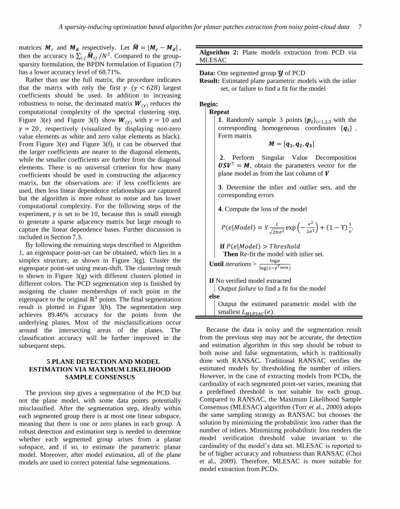
Because the data is noisy and the segmentation result

from the previous step may not be accurate, the detection

and estimation algorithm in this step should be robust to

both noise and false segmentation, which is traditionally

done with RANSAC. Traditional RANSAC verifies the

estimated models by thresholding the number of inliers.

However, in the case of extracting models from PCDs, the

cardinality of each segmented point-set varies, meaning that

a predefined threshold is not suitable for each group.

Compared to RANSAC, the Maximum Likelihood Sample

Consensus (MLESAC) algorithm (Torr et al., 2000) adopts

the same sampling strategy as RANSAC but chooses the

solution by minimizing the probabilistic loss rather than the

number of inliers. Minimizing probabilistic loss renders the

model verification threshold value invariant to the

cardinality of the model’s data set. MLESAC is reported to

be of higher accuracy and robustness than RANSAC (Choi

et al., 2009). Therefore, MLESAC is more suitable for

model extraction from PCDs.

Algorithm 2: Plane models extraction from PCD via

MLESAC

Data: One segmented group of PCD

Result: Estimated plane parametric models with the inlier

set, or failure to find a fit for the model

Begin: Repeat

1. Randomly sample 3 points with the

corresponding homogeneous coordinates .

Form matrix

2. Perform Singular Value Decomposition

, obtain the parameters vector for the

plane model as from the last column of

3. Determine the inlier and outlier sets, and the

corresponding errors

4. Compute the loss of the model

( )

√ (

) ( )

.

If ( )

Then Re-fit the model with inlier set.

Until iterations >

( )

If No verified model extracted

Output failure to find a fit for the model

else

Output the estimated parametric model with the

smallest ( ).

Zhang et al. 8

5.1 Planes detection and estimation from PCDs

MLESAC first randomly samples a subset of points with

the minimum cardinality needed for model estimation,

then the sampled subset is used to fit a parametric model.

For plane estimation, . Denote the three points

sampled by , then the plane parameters

are obtained from the following steps. First express in

homogeneous form as , then form the matrix

(11)

Perform singular value decomposition of , which

estimates both the normal and the offset of the plane:

(12)

The hypothesized parameter vector of the

plane is obtained from the fourth column of with

normalization by dividing the additive inverse of the last

element.

MLESAC evaluates the fitness of the hypothesis using a

probabilistic model for the errors arising from inliers and

outliers. The inlier error is modeled as unbiased Gaussian

distribution while the outlier error as uniform distribution.

Hence the probability of the error given the estimated

model is:

( )

√ (

) ( )

(13)

where is the inlier error, is the prior probability of

being an inlier (the ratio of inlier), is the size of available

error space, is the standard deviation of Gaussian noise. If

( ) is larger than the threshold, then the model

will be re-estimated using only the inliers and MLESAC

terminates. Otherwise, repeat the process with another

random sample set, compute the loss, and determine if a

further iteration is needed. The maximum number of

iterations to perform is

( ) (14)

where is the estimated failure probability of picking up

inlier samples at least once. The MLESAC loop terminates

when the required iterations have been finished.

The plane model estimation step is summarized in

Algorithm 2. The estimation results of this step correct

erroneously segmented points from the previous step by

relabeling each point to the model with the minimum

Euclidean distance between the point and the model. Pairs

of estimated models are merged togethor if the parametric

models are close and the point set supports are adjacent.

5.2 Illustration of Algorithm 2 on the synthetic PCD

Algorithm 2 is illustrated using the same synthetic PCD

discussed in Section 4.3. In the plane models extraction

step, points from each group are processed using Algorithm

2. For MLESAC, the threshold for the probability

( ) is set to be 0.5, which is optimized

empirically. The inlier set and outlier set detected for each

segmented group are plotted in Figure 4(a), in which black

‘ ’ signs stand for inliers and red ‘ ’ signs stand for

outliers. The models extracted for the three groups are

reported in Table 1 with the absolute errors computed by

comparing to the ground truth. It can be concluded that the

planar models extracted are of high accuracy. These

extracted models are further used as feedback to improve

the segmentation results by assigning all the points to the

model to which the perpendicular Euclidean distance is the

smallest among all the models and smaller than a

predefined threshold (in this experiment the threshold is

0.1), and the points whose perpendicular distances are

larger than the threshold are labeled as noise. The

segmentation result after this assignment is illustrated in

Figure 4(b), which has 93.79% accuracy for the whole

PCD.

Table 1 Experiment results, ground truth and absolute errors of the model estimation step in the synthetic PCD experiment (the plane

models are evaluated using the normalized plane equation .)

Planes Item Parameters of Plane Models

Plane 1

Experiment Result Ground Truth

Absolute Error

Plane 2


Absolute Error

Plane 3


Absolute Error


6 Determine Plane Boundaries via QR Decomposition

based Projected -Shape

After the previous two steps, the segmentation of the

points from different planes and the corresponding planar

models have been obtained. Generating the final

representations for the planar patches requires identifying

the boundary each extracted planar patch. The challenges of

this step are: (1) the boundary point-sets may not be

convex; instead they may be concave or even with openings

inside the outer “ boundary ”; (2) points in each point-set

may not be uniformly distributed; and (3) the points are

corrupted with noise.

6.1 Maximum projected variance -shape algorithm

To resolve these problems, some methods have been

proposed for determining the boundary point-set. (Truong-

Hong et al., 2013) proposed to combine an angle criterion

and the Flying Voxel method for boundary determination,

but it works better in less dense point-sets (<175

points/ ). The -shape algorithm (Akkiraju et al., 1995)

is effective at determining the boundary of large point-sets.

The algorithm has been successfully applied to boundary

extraction of roof planes from aerial view generated PCDs

(Dorninger et al., 2008). Because roofs are of small angle

w.r.t. the ground, 3D points are simply projected onto the

grouped plane and then -shape is applied to extract

boundary. In this method, no selection of projecting plane

are needed and the projecting plane is simply set as the

ground plane. In our case the poses (positions and

orientations) of planes are arbitrary. Prior to applying the

2D -shape algorithm to 3D planes in arbitrary poses, the

3D points of planes should be transformed to a 2D

coordinate representation. While there are a variety of ways

to construct an orthogonal frame for the plane, we describe

here a QR decomposition approach based on the estimated

plane normal.

Given a PCD point-set and its estimated

normal , first a matrix is

formed, where are random column vectors

generated from the point-set. Then QR decomposition of

is:

(15)

where is an orthogonal matrix.

The natural coordinate vectors are given by the three

column vectors of . In this work, the

in the natural coordinate frame is defined with

(the plane normal), with and with

. Then project onto the natural coordinates by

(16)

where the factor projects 3D points to 2D

points. The arrangement of columns in performs a ( ) transformation aligning the normal

vector of plane in the original frame to the in the

projected frame.

The projected point-set is obtained by .

The overall algorithm for plane projection and boundary

detection via -shape is found in Algorithm 3. The -shape

algorithm is then performed on . Since the boundary

detected depends on the radius of the circles (or value),

here we set the value as 3 times of the average single-link

(a) Inlier (black ‘ ’) and outlier

(red ‘ ’) set obtained in

MLESAC

(b) PCD segmentation after

MLESAC re-correction

Figure 4: Illustration of Algorithm 2 on the synthetic PCD

Algorithm 3: Plane boundary detection via maximum

projected variance -shape algorithm

Data: A PCD point-set on a detected plane

and the estimated plane normal

Result: 3D boundary point-set

Begin: 1. Form a matrix

;

where are random column vectors

2. Perform QR decomposition on :

3. Define the natural coordinate frame with

and project onto the frame by:

;

;

where is the projected point-set

4. Get -shape boundary of ;

5. Determining the 3D plane boundary point-set

by retrieving the membership of the 2D boundary

point-set.

Zhang et al. 10

point-point distance, which is a conclusion assessed

experimentally. The boundary detected using this value is

shown in Figure 5(a). The 2D boundaries are then projected

back to the 3D space, shown in Figure 5(b). This outside

concave boundary is detected without any additional

boundaries for the openings inside the point set. performs a

( ) transformation aligning the normal vector of plane

in the original frame to the in the projected frame.

The projected point-set is obtained by

. The overall algorithm for plane projection and

boundary detection via -shape is found in Algorithm 3.

The -shape algorithm is then performed on . Since the

boundary detected depends on the radius of the circles (or

value), here we set the value as 3 times of the average

single-link point-point distance, which is a conclusion

assessed experimentally. The boundary detected using this

value is shown in Figure 5(a). The 2D boundaries are

then projected back to the 3D space, shown in Figure 5(b).

This outside concave boundary is detected without any

additional boundaries for the openings inside the point set.

6.2 Illustration of Algorithm 3 on a synthetic PCD

As the final step, the boundaries of each extracted planes

are detected by performing Algorithm 3 on each segmented

group. The detected boundaries are plotted out in Figure

6(a). Finally, the planar patches representation is generated

as shown in Figure 6(b).

7 EVALUATION OF THE PROPOSED

ALGORITHM

7.1 Memory and time complexities

The complexity of the proposed method is analyzed in

terms of the memory complexity and computation

complexity. The most memory consuming part of the

algorithm is the storage of the adjacency matrix in

Algorithm 1. The size of is at most , where is the

number of points in PCD and is the number linear

dependence coefficients kept. Thus, the memory

complexity is ( ) with a data structure for sparse

matrix/graph, e.g. CSR (Compressed Spared Row Graph).

The time complexity is determined by the most expensive

steps, which are the group-sparsity optimization

programming and the eigen-decomposition steps in

Algorithm 1. These steps both require cubic time of the

input data size. Since a partitioning strategy is used on the

PCD before performing the algorithm (see Section 8.1.2),

the time complexity is reduced. Given as the number of

parts the PCD is partitioned into and assume that the PCD

is quite uniformly distributed in different parts (and for

simplicity, assume each part has roughly the same number

of points), the expected running time for each part is

(

). Assuming the parts are processed sequentially,

the final time complexity is (

) . If the parts are

processed concurrently on a parallel machine with

processes, the time complexity is further reduced to

(⌈

⌉

) for or (

) for .

7.2 Evaluation metrics

To evaluate the complete plane identification and

extraction algorithm, five different evaluation metrics will

be computed. These metrics evaluate different aspects of

the algorithm performance to give a comprehensive

understanding of how well models detected and extracted.

These metrics and their purpose are as follows: Root Mean

Square error measures the model fitting accuracy; Normal

Deviation measures the orientation accuracy; Unit Volume

error measures both the orientation and the translation

accuracy; Detection Percentage measures what percentage

of the total number of patches were detected;

Oversegmentation Factor gives the factor by which the

planar models overrepresent the ground-truth models.

7.2.1 Root mean square error (RMSE)

The RMSE measures the consistency of the model to the

data. For every point that belongs to an extracted

plane with the model , where is

the normal of the plane with unit length and is the offset

of the plane. The point-plane distance is then measured by

(17)

(a) Boundary extracted on

the projected 2D point set

(b) Boundary back-projected

to 3D space

Figure 5 Boundaries found using QR decomposition based

projected -Shape algorithm (Radius= )

(a) Detected boundaries of

extracted planes

(b) Final planar patches

representation

Figure 6: Illustration of Algorithm 3 on synthetic PCD


The root mean square error (RMSE) for each extracted

plane is defined as

√

∑ ( ) (18)

where is the index of the points that

associated to the plane.

7.2.2 Normal deviations

The normal deviation measures the accuracy of

orientation between the extracted plane compared to the

ground-truth plane. Given the normal vector of an

estimated plane and the corresponding ground-truth normal

vector , the normal deviation is:

( ) (19)

7.2.3 Unit volume error

Besides orientation accuracy, the localization accuracy

of the plane is important. Accordingly, here we define an

evaluation metric which captures both the orientation and

translation accuracy, the unit volume error. It is the volume

generated from the estimated patch and the ground-truth

patch divided by the area of the ground-truth patch. The

volume error is illustrated in Figure 7. The volume is

defined in the direction orthogonal to the ground-truth

patch. In the calculation of the volume, absolute distances

are used instead of the signed distances. The units of this

score are .

(20)

7.2.4 Detection percentage

This metric evaluates how completely the algorithm is

able to detect all existing planar patches in the PCD. It is

the percentage of the number of extracted patches, relative

to the quantity of patches in the ground truth model. The

number of extracted patches is defined as the number of

patches in the ground-truth data that are correctly found by

the algorithm. For example, if there are 20 planar patches in

the whole ground-truth PCD, and the algorithm is able to

extract 12 out of the 20 planar patches, then the Detection

Percentage is 60%. Moreover, if patch A in the ground-

truth data is found but broken into two patches by the

algorithm, patch A is counted as one patch extracted; or if

only a part of patch A is found by the algorithm, it is still

counted as one extracted patch. The ideal value is 100%.

7.2.5 Oversegmentation factor

This metric aims to evaluate for a detected ground-truth

planar patch, how well the procedure models the patch. For

each ground-truth planar patch, the number of the

corresponding extracted planes is counted. Then the

oversegmentation factor is defined to be the quantity of

extracted plane models divided by the quantity of unique

ground-truth models associated to them. For example,

suppose that the procedure detected six planar patches, two

Figure 7 Volume between two planar patches

(a) Our method (b) (Okorn et al., 2010)

(c) (Budroni et al., 2009) (d) (Adan et al., 2011)

Figure 8 Final results using different methods on the synthetic PCD

Table 2 Evaluation results on the synthetic PCD

Methods our method (Okorn et al.,

2010)

(Budroni et al.,

2009)

(Adan et al.,

2011)

RMSE (cm) 2.17 0.61 6.91 1.57 7.95 2.12 1.20 1.46

Unit Volume Err. ( ) 0.13 0.02 0.32 0.08 0.37 0.11 0.13 0.25

Normal Deviations ( ) 0.14 0.12 0 0 17.98 21.47

Detection Percentage 100% 100% 100% 100%

Oversegmentation Factor 1 1 1 1

Zhang et al. 12

belonging to one ground truth model, and four belonging to

a second ground truth model. Then the oversegmentation

factor is ( ) . Combining Detection Factor, the

ideal case is that the oversegmentation factor equals to 1

and the detection percentage equals to 100%. In this case,

there is a one-to-one mapping from the estimated patches to

the ground-truth patches.

7.3 Overall performance of the proposed algorithm on

the synthetic PCD

Using the evaluation metrics, the proposed algorithm is

compared to three baseline algorithms. The three baseline

methods are the Hough transform based algorithm of

(Okorn et al., 2010), the plane-sweeping algorithm of

(Budroni et al., 2009), and the region-growing based

method of (Adan et al., 2011). Some of these algorithms

only address parts of the pipeline of this problem. In order

for a fair comparison, the parts in the pipeline which are not

solved by the compared algorithms will be addressed using

the corresponding steps of the proposed algorithm.

Moreover, the final planar patch representations of these

methods are different. For method (Okorn et al., 2010) and

method (Budroni et al., 2009) the final results are in solid

planar patches, while for method (Adan et al., 2011) the

final results are segmentations of points. The results of

these three methods on the synthetic PCD are shown in

Figure 8 respectively. The evaluation results are shown in

Table 2, which are presented in the format of “mean

standard deviation”, because there are multiple planes in the

dataset and the statistics are computed over the planes. This

simple, synthetic PCD example does not fully reflect real-

world PCDs. For example, the real-world dataset may not

be oriented precisely, which would introduce errors when

using methods in (Okorn et al., 2010) and (Budroni et al.,

2009).

In Table 2, the methods (Okorn et al., 2010) and

(Budroni et al., 2009) have RMSE>0 but the normal

deviations are zeros because the extracted planes are of an

offset compared to the ground-truth planes but they are also

parallel to the ground-truth planes (and this is why the

normal deviations are exactly zeros). Note that the normal

deviations of (Okorn et al., 2010) and (Budroni et al., 2009)

can be zeros because in this synthetic example all the planes

are placed perfectly parallel to the coordinate planes. These

two methods rely on the projection onto coordinate planes

or plane-sweeping along the direction from rotational

sweeping. Thus, they have zero normal deviations in this

synthetic example. However, in reality, the planes in point-

clouds may not perfectly align with the coordinate planes or

the extracted direction. Therefore in the real-world PCDs

example, these two methods do not have zero normal

deviations. It is worthy to note that none of these compared

methods is able to give estimated plane models or the

detailed boundaries. Especially, the region-growing based

methods are only able to give segmentation of point clouds

that ideally belong to some planes.

We end the discussion for the synthetic PCD experiment

by investigating the influence of the number (denoted as )

of linear dependence coefficients used in constructing the

similarity graph. The misclassification rates of the PCD

segmentation step w.r.t. from 2 to 627 are plotted in

Figure 9. As it can be observed, the mis-classification rate

varies between and . Given that the model

fitting step corrects this error, the change in performance as

a function of is not significant enough to warrant using

large values of the parameter . Thus, it is recommended to

use a relatively small , one which would correspond to

selecting a small percentage of the total dataset.

8 EXPERIMENTS AND EVALUATIONS ON REAL-

WORLD CIVIL INFRASTRUCTURES PCD

This section evaluates the performance of the proposed

algorithm when applied to two real-world infrastructures

PCDs. The real-world PCDs used were captured using two

different kinds of methods: a building PCD reconstructed

from videos using Structure-from-Motion methods, and a

bridge PCD captured directly using a laser scanner. These

two real-world PCDs are both of civil infrastructures but

with different levels of noise.

When dealing with large-scale PCDs, some pre-

processing and post-processing steps can be added to help

reduce the processing time. First, the PCD is cut into

multiple smaller PCDs by partitioning the volume into

smaller volumes. The proposed procedure is applied to each

partition. After extracting all planar patch models, the post-

processing step merge the patches that are adjacent and

have low difference in the model parameters. These pre-

processing and post-processing steps are used in the

experiments in Section 8.

8.1 Experiment 1: building dataset from video

8.1.1 Point cloud dataset

In this experiment, the PCD of a real building is used.

The PCD is reconstructed from video using the open-source

3D reconstruction tool PMVS2 (Furukawa et al., 2010). A

Figure 9 Misclassification rate w.r.t. different numbers of

linear elements in constructing the similarity graph


frame from the video is shown in Figure 10. Due to the

physical constraints of the environment, only three faces of

the building were captured. Moreover, there are some

occlusions in the scene, e.g., trees, decorations, etc. The

reconstructed raw PCD is displayed in Figure 11. The point

cloud consists of 1,681,634 points, with relatively large

measurement uncertainty.

8.1.2 Experimental results

The building PCD is processed using the proposed

algorithm, with parameter settings as listed in Table 3. To

lower the computational complexity, the PCD is first

partitioned into parts. The final result of

the experiment, after merging the partition results, is shown

in Figure 12(a), (b). The algorithm extracts 16 planar

patches from the PCD.

The raw PCD is also plotted in Figure 12(a), (b) in

magenta to provide intuitive comparison between the raw

point cloud and the extracted patches. Note that some open

parts (for instance, the intersecting part between two roof

planes in Figure 12 (b)) exist because the point cloud itself

does not capture the corresponding part due to some

occlusions. From the experiment it can be observed that the

extracted patches fit with the point cloud very well.

8.1.3 Comparison to baseline methods

For (Okorn et al., 2010) method, since proper orientation

is required, the orientation of the PCD is corrected to align

the walls to coordinate axes before conducting the

experiment. The parameters of the compared methods are

as follows. For (Okorn et al., 2010), we set the grid size of

the 2D histogram as . For (Budroni et al.,

(a) Our method (view 1) (b) Our method (view 2) (c) Method in (Okorn et al.,

2010) (view 1)

(d) Method in (Okorn et al.,

2010) (view 2)

(e) Method in (Budroni et

al., 2009) (view 1)

(f) Method in ( Budroni et

al., 2009) (view 2)

(g) Method in (Adan et al.,

2011) (view 1)

(h) Method in (Adan et al.,

2011) (view 2)

Figure 12 Extracted planar patches for the building PCD using different methods, plotted with the raw PCD (in magenta)

Figure 10 A sample image from video used to reconstruct

a building

Figure 11 Raw PCD representation of a building

Table 3

Parameter configurations for the building PCD

experiment

Parameters Value

optimization parameter 1

optimization parameter 1

number of coefficients used in adjacency matrix 10

MLESAC verification probability threshold 0.5

MLESAC false alarm rate

1e-3 (probability a good minimal sample set never

picked)

MLESAC assumed noise standard deviation 0.1

MLESAC minimum iterations 1000

Point-model distance threshold for Re-

segmentation

0.1

Zhang et al. 14

2009) method, the number of the bins used to generate the

histogram of point numbers for sweeping is 200 and the

threshold to define a plane in the histogram is set to be half

of the maximum value in the histogram. For (Adan et al.,

2011) method, the PCD is voxelized into grids. The number of neighbour points for normal

estimation is 50; the threshold of maximum angle between

normal vectors is 2 degrees; the curvature threshold to

guarantee points are well-described by plane models is set

as 1. All of these parameter configurations are optimized

empirically.

Ground-truth data of the building is collected using a

professional total station (i.e., SOKKIA 30R). Points are

measured for each facet of the infrastructures, especially the

points that define the boundary of each facet of the

infrastructure. The PCD is obtained by merging the point-

sets from different scan domains using the software of the

total station. Another method of merging point-sets from

multiscan domains is proposed in (Sareen et al., 2012) for

generating more consistent PCDs. After collecting the PCD,

the measured points belonging to each specific facet are

selected manually and used to generate the ground-truth

data for each facet. The planes measured as ground-truth

are shown in Figure 13. These planes are used to evaluate

RMSE, unit volume error and normal deviations. For

detection percentage and oversegmentation factor, in total

14 planes are considered. The experiment is evaluated using

the evaluation metrics defined in Section 7.1.

The evaluation results of the proposed procedure and the

three baseline procedures are listed in Table 4. Note that in

Table 4, method (Budroni et al., 2009), no standard

deviation is given because the method only extracts one

patch that can be considered corresponding to a ground-

truth plane, which is the largest wall of the building. Since

only one extracted patch is considered to have a

corresponding ground-truth patch, we only have one value

for each metric and undefined standard deviation.

From Table 4 it can be concluded that the proposed method

has the best performance among all the comparative

methods.

8.2 Experiment 2: bridge dataset from laser scanner

8.2.1 Point cloud dataset

This section applies the algorithm to the PCD of a bridge

captured using a professional laser scanner (Leica Laser

Scan Total Station C10). The bridge span is more than 200

meters. The raw PCD has 2,005,582 points, which are

shown in Figure 14. Compared to the building dataset, this

PCD is of higher accuracy. Moreover, this PCD has more

planar patch elements then the building PCD. In total, there

are 40 patches (2 for the road surfaces, 2 for the left and

right span along the road surface, 9 square columns with 36

planar patches in total). Since the upper surfaces and the

lower surfaces coincide with the big upper and lower planes

of span of the bridge, we decided to only count the planes

of the span instead of the planes of the beams to avoid

confusions. The surfaces on the floor and the ramp are not

considered in this experiment because they are not parts of

the infrastructure components. The proposed procedure and

the baseline methods are tested on this PCD.

Figure 13 Planes measured using total stations to

provide ground truth data

Figure 14 Point-cloud representation of the raw

bridge PCD

Table 4 Evaluation results on the building PCD


2010)

(Budroni et al.,

2009)

(Adan et al., 2011)

RMSE ( ) Unit Volume Err. ( ) Normal Deviations ( ) Detection Percentage Oversegmentation Factor


8.2.2 Experimental results

The results on the bridge PCD using the proposed

algorithm and the same partition strategy as in the previous

experiment are shown in Figure 15(a), (b). In total there are

29 planar patches extracted excluding the patches for the

floor and the ramp. The completeness in terms of the

number of planar patches is . The extracted

patches cover the horizontal and the vertical surfaces of the

road parts, and most of the surfaces (25 out of 36 patches)

on all the columns. For the patches of the columns which

the algorithm fails to extract, it can be observed from the

raw PCD that the point densities for these patches are lower

than for the detected column patches, because the positions

of these patches are blocked in some of the laser scan

views. The ground-truth data of this PCD is generated

manually from laser total station data. The performance is

validated using the metrics in Section 7.1 and the evaluation

statistics are listed in Table 5 in details. It can be concluded

from table that the proposed algorithm achieves high

accuracy in all of these three metrics, and the result on this

PCD is more accurate than the result on the building PCD.

8.2.3 Comparison to baseline methods

The parameters configured are as follows. For (OKorn et

al, 2010), we set the grid size of the 2D histogram as 0.3m x

0.3m. For (Budroni et al, 2009), the parameters are the

same as the previous experiment. For (Adan et al., 2011)

method, voxel grid size is 3.5 . The

number of neighbour points for normal estimation is 100;

the angle threshold is 2 degrees; the curvature threshold is

1.5. Again, these parameters were optimized empirically

according multiple trails of experiments.

The results of the baseline method are also found in

Figure 15. The result of (Okorn et al., 2010) is shown in

Figure 15(c) (d), the result of (Budroni et al., 2009) is in

Figure 15 (e) (f), and the result of (Adan et al., 2011) is in

Figure 15 (g) (h).

Evaluation statistics for all the procedures are listed in

Table 5. The proposed method achieves the best

performance in terms of all the metrics except for the

RMSE. For the RMSE, the method in (Adan et al., 2011)

has the smallest mean value, while the RMSE of the

proposed method is slightly larger than the method in

(Adan et al., 2011) but with smaller standard deviation of

RMSE than method in (Adan et al., 2011) which means the

RMSEs of all the extracted planes for the proposed method

are more consistent than that for method in (Adan et al.,

2011). It can also be observed that (Adan et al., 2011)

method has larger oversegmentation factor compared to the

proposed method, which is because it breaks the bridge

surface into several patches. In addition, it is worthy to note

(a) Our method (view 1) (b) Our method (view 2) (c) Method in (Okorn et al.,

2010) (view 1)

(d) Method in (Okorn et al.,

2010) (view 2)

(e) Method in (Budroni et

al., 2009) (view 1)

(f) Method in (Budroni et

al., 2009) (view 2)

(g) Method in (Adan et al.,

2011) (view 1)

(h) Method in (Adan et al.,

2011) (view 2)

Figure 15 Extracted planar patches for the bridge PCD using different methods, plotted with the raw PCD (in magenta)

Table 5 Evaluation results on the bridge PCD


2010)

(Budroni et al.,

2009)

(Adan et al.,

2011)

RMSE ( ) Unit Volume Err. ( ) Normal Deviations ( ) Detection Percentage Oversegmentation Factor

-200

-150

-100

-50

0

50

100

-120-100

-80-60

-40-20

-40

-20

0

20

40

60

-200

-150

-100

-50

0

50

100-120

-100-80

-60-40

-20

-40

-20

0

20

40

60

Zhang et al. 16

that (Adan et al., 2011) method gives false positives in the

final result and more importantly the outputs of this method

are segmentations of the input PCD with no estimates of the

plane models nor the planar patch boundaries. In general, it

can be concluded the proposed method has better overall

performance among all the comparative methods.

9 CONCLUSION

This work focuses on the problem of planar model

extraction from civil infrastructure PCDs, which requires

three objectives including the detection of planar structures,

estimation of planar parametric models and determination

of the planar model boundaries. In this paper, an innovative

algorithm is proposed for addressing this problem. The

proposed procedure is demonstrated to be suitable for large-

scale noisy infrastructure PCDs and able to address all the

three objectives. One of the most important steps of this

procedure is that it first recovers the linear dependence

relationship between each point in the PCD, by solving a

group-sparsity inducing optimization program. With the

recovered linear dependence coefficients, the algorithm

further segments the PCD by clustering the points

according to the linear subspace. The clustering uses

spectral clustering with a similarity graph formed from the

linear dependence coefficients matrix. After PCD

segmentation, planes are detected and estimated for each

segmented group via an SVD based approach using

MLESAC. Finally, the boundary of each plane is detected

using the -shape algorithm. The proposed algorithm is

tested extensively using three types of PCDs: synthetic

data, a PCD of a real building reconstructed from video,

and a PCD of a bridge captured directly using laser

scanners. For the synthetic PCD experiment, detailed

results are provided to illustrate every step of the procedure.

To comprehensively evaluate the model extraction

performance, five different evaluation metrics are applied.

Furthermore, the proposed algorithm is also compared with

three baseline methods. The experimental results and the

evaluation statistics on the real-world PCDs demonstrate

that the proposed algorithm has the best overall

performance among the comparative methods on the real-

world PCDs. The future work includes the extension of the

proposed algorithm for extracting more geometric shapes

embedded in PCDs, and recognizing the infrastructure

components after model extraction.

REFERENCES

Adan, A., Xiong, X., Akinci, B., & Huber, D. (2011),

Automatic Creation of Semantically Rich 3D Building

Models from Laser Scanner Data. Proceedings of the

International Symposium on Automation and Robotics in

Construction (ISARC), pp. 342-347.

Agarwal P. & Mustafa, N. (2004), K-means Projective

Clustering, Proceedings of ACM SIGMOD-SIGACT-

SIGART Symposium Principles of Database Systems, pp.

155-165.

Akkiraju, N., Edelsbrunner, H., Facello, M., Fu, P.,

Mucke, E. P. & Varela, C. (1995), Alpha Shapes:

Definition and Software, Proceedings of International

Computational Geometry Software Workshop, pp. 63-66.

Bosché, F. (2012), Plane-based Registration of

Construction Laser Scans with 3D/4D Building Models.

Advanced Engineering Informatics, 26(1), pp. 90-102.

Budroni, A. & Jan B. (2009), Toward Automatic

Reconstruction of Interiors from Laser Data, Proceedings of

the Workshop on 3D Virtual Reconstruction and

Visualization of Complex Architectures.

Choi, S., Kim, T. & Yu, W. (2009), Performance

Evaluation of RANSAC Family, Proceedings of the British

Machine Vision Conference.

Comaniciu, D. & Meer, P. (2002), Mean shift: A Robust

Approach Toward Feature Space Analysis, Pattern Analysis

and Machine Intelligence, IEEE Transactions on, 24(5), pp.

603–619.

Costeira, J. & Kanade, T. (1998), A Multibody

Factorization Method for Independently Moving Objects,

Internaional Journal of Computer Vision, 29(3), pp. 159-

179.

Davison, A. J., Reid, I. D., Molton, N. D. & Stasse, O.

(2007), MonoSLAM: Real-Time Single Camera SLAM,

Pattern Analysis and Machine Intelligence, IEEE

Transactions on, 29(6), pp. 1052-1067.

Deshpande, S.S. (2013), “Improved Floodplain

Delineation Method Using High Density LiDAR Data,”

Computer-Aided Civil and Infrastructure Engineering,

28(1), pp. 68-79.

Donoho, D. L. (2006), For Most Large Underdetermined

Systems of Linear Equations the Minimal -norm Solution

Is Also the Sparsest Solution. Communications on Pure and

Applied Mathematics, 59(6), pp. 797-829.

Dorninger, P., & Pfeifer, N. (2008), A Comprehensive

Automated 3D Approach for Building Extraction,

Reconstruction, and Regularization from Airborne Laser

Scanning Point Clouds. Sensors, 8(11), pp. 7323-7343.

Elhamifar, E. & Vidal, R. (2009), Sparse Subspace

Clustering, Proceedings of the IEEE Conference on

Computer Vision and Pattern Recognition, pp. 2790-2797.

Farin, G. (1992), From Conics to NURBS: A Tutorial

and Survey, IEEE Computer Graphics and Applications,

12(5), pp. 78-86.

Farin, G. (1996), Curves and Surfaces for Computer

Aided Geometric Design: A Practical Guide (4th edition),

Academic Press, Boston, Massachusetts.

Fischler, M. A. & Bolles, R. C. (1981), RANdom

SAmple Consensus: A Paradigm for Model Fitting with

Applications to Image Analysis and Automated


Cartography. Communications of the ACM, 24(6), pp. 381-

395.

Furukawa, Y. & Ponce, J. (2010), Accurate, Dense, and

Robust Multiview Stereopsis, Pattern Analysis and

Machine Intelligence, IEEE Transactions on, 32(8), pp.

1362-1376.

Goedert, J., Bonsell, J. & Samura, F. (2005), Integrating

Laser Scanning and Rapid Prototyping to Enhance

Construction Modeling, Journal of Architecture

Engineering, 11(2), pp. 71-74.

Hähnel, D., Burgard, W. & Thrun, S. (2003), Learning

Compact 3D Models of Indoor and Outdoor Environments

with a Mobile Robot, Robotics and Autonomous Systems,

44(1), pp. 15-27.

Huber, D., Akinci, B., Oliver, A., Anil, E., Okorn, B. &

Xiong, X. (2011), Methods for Automatically Modeling and

Representing As-built Building Information Models,

Proceedings of the NSF CMMI Research Innovation

Conference.

Landes, T. & Grussenmeyer P. (2007), Hough-transform

and Extended RANSAC Algorithms for Automatic

Detection of 3D Building Roof Planes from LiDAR Data,

Science and Technology, 36(1), pp. 407-412.

Liu, G., Lin, Z. & Yu, Y. (2010), Robust Subspace

Segmentation by Low-rank Representation, Proceedings of

Internaional Conference of Machine Learning, pp. 663–670

Lu, L. & Vidal, R. (2006), Combined Central and

Subspace Clustering on Computer Vision Applications,

Proceedings of International Conference of Machine

Learning, pp. 593-600.

Ma, Y., Derksen, H., Hong, W. & Wright, J. (2007),

Segmentation of Multivariate Mixed Data via Lossy Coding

and Compression, Pattern Analysis and Machine

Intelligence, IEEE Transactions on, 29(9), pp. 1546-1562.

Martín Nevado, M., Gómez García-Bermejo, J., &

Zalama Casanova, E. (2004), Obtaining 3D models of

indoor environments with a mobile robot by estimating

local surface directions. Robotics and Autonomous

Systems, 48(2), pp. 131-143.

Ng, A. Y., Jordan, M. I. & Weiss, Y. (2002), On Spectral

Clustering: Analysis and An Algorithm, Advances in neural

information processing systems, pp. 849-856.

Okorn, B., Xiong, X., Akinci, B. & Huber, D. (2010),

Toward Automated Modeling of Floor Plans, Proceedings

of the Symposium on 3D Data Processing, Visualization

and Transmission.

Pollefeys, M., Nister, D., Frahm, J. M., Akbarzadeh, A.,

Mordohai, P., Clipp, B., Engels, C., Gallup, D., Kim, S. J.,

Merrell, P., Salmi, C., Sinha, S., Talton, B., Wang, L.,

Yang, Q., Stewenius, H., Yang, R., Welch, G. & Towles, H.

(2008), Detailed Real-time Urban 3D Reconstruction from

Video, International Journal of Computer Vision, 78(2-3),

pp. 143-167.

Rao, S., Tron, R., Ma, Y., & Vidal, R. (2008), Motion

Segmentation via Robust Subspace Separation in the

Presence of Outlying, Incomplete, or Corrupted

Trajectories, Proceedings of the IEEE Conference on

Computer Vision and Pattern Recognition, pp. 1-8.

Sareen, K. K., Knopf, G. K. & Canas, R. (2012),

Consistent Point Clouds of Narrow Spaces using Multiscan

Domain Mapping, Computer-Aided Civil and Infrastructure

Engineering, 27(8), pp. 555-638.

Schnabel, R., Wahl, R. & Klein, R. (2007), Efficient

RANSAC for Point-Cloud Shape Detection, Computer

Graphics Forum, 26(2), pp. 214-226.

Seitz, S. M., Curless, B., Diebel, J., Scharstein, D. &

Szeliski, R. (2006), A Comparison and Evaluation of Multi-

View Stereo Reconstruction Algorithms, Proceedings of the

IEEE Conference on Computer Vision and Pattern

Recognition, pp. 519-528.

Stamos, I. & Allen, P. E. (2000), 3-D Model

Construction using Range and Image Data, Proceedings of

the IEEE Conference on Computer Vision and Pattern

Recognition, vol. 1, pp. 531-536.

Soltanolkotabi, M. & Candes, E. J. (2012), A Geometric

Analysis of Subspace Clustering with Outliers, The Annals

of Statistics, 40(4), pp. 2195-2238.

Tarsha-Kurdi, F., Landes, T. & Grussenmeyer, P. (2008),

Extended RANSAC Algorithm for Automatic Detection of

Building Roof Planes from LiDAR DATA,

Photogrammetric Journal of Finland, 21(1), pp. 97-109.

Thrun, S., Martin, C., Liu, Y., Hahnel, D., Emery-

Montemerlo, R., Chakrabarti, D. & Burgard, W. (2004), A

Real-time Expectation-maximization Algorithm for

Acquiring Multi-planar Maps of Indoor Environments with

Mobile Robots, Robotics, IEEE Transactions on, 20(3), pp.

433-443.

Torr, P. H. & Zisserman, A. (2000), MLESAC: A New

Robust Estimator with Application to Estimating Image

Geometry, Computer Vision and Image Understanding,

78(1), pp. 138-156.

Triebel, R., Burgard, W. & Dellaert, F. (2005), Using

Hierarchical EM to Extract Planes from 3D Range Scans,

Proceedings of the 2005 IEEE International Conference on

Robotics and Automation, pp. 4437-4442.

Truong-Hong, L., Laefer D. F., Hinks, T. & Carr, H.

(2013), Combining an Angle Criterion with Voxelization

and the Flying Voxel Method in Reconstructing Building

Models from LiDAR Data, Computer-Aided Civil and

Infrastructure Engineering, 28(2), pp. 112-129.

Vidal R., Ma Y. & Sastry, S. (2005), Generalized

Principal Component Analysis (GPCA), Pattern Analysis

and Machine Intelligence, IEEE Transactions on, 27(12),

pp. 1-15.

Vidal, R. (2011), Subspace Clustering, IEEE Signal

Processing Magazine, 28(2), pp. 52-68.

Vosselman, G. (2009), Advanced Point Cloud Processing.

Photogrammetric Week, vol. 9, pp. 137-146.

Walsh, S. B., Borello, D. J., Guldur, B., & Hajjar, J. F.

(2013). Data Processing of Point Clouds for Object

Zhang et al. 18

Detection for Structural Engineering Applications.

Computer Aided Civil and Infrastructure Engineering,

28(7), pp. 495-508.

Zhang, C. and Elaksher, A. (2012), “An Unmanned

Aerial Vehicle-Based Imaging System for 3D Measurement

of Unpaved Road Surface Distresses,” Computer-Aided

Civil and Infrastructure Engineering, 27(2), pp. 118-129.

Zhang, G., Karasev, P., Brilakis, I., & Vela, P. A. (2012),

A Sparsity-inducing Optimization Algorithm for the

Extraction of Planar Structures in Noisy Point-cloud Data.

Proceedings of ASCE International Workshop on

Computing in Civil Engineering, pp. 317-324.

Zhang, T., Szlam, A. & Lerman, G. (2009), Median K-

flats for Hybrid Linear Modeling with Many Outliers,

Proceedings of Workshop of Subspace Methods, pp. 234-

241.

Zhang, T., Szlam, A., Wang, Y. & Lerman, G. (2010),

Hybrid Linear Modeling via Local Best-fit Flats,

Proceedings of the IEEE Conference on Computer Vision

and Pattern Recognition, pp. 1927-1934.

A sparsity-inducing optimization based algorithm for ...

Documents

Transcript of A sparsity-inducing optimization based algorithm for ...