A Sparsi cation Based Algorithm for Maximum-Cardinality ... · planar graph with nvertices and...

A Sparsification Based Algorithm for Maximum-Cardinality

Bipartite Matching in Planar Graphs

Mudabir Kabir Asathulla

Thesis submitted to the Faculty of the

Virginia Polytechnic Institute and State University

in partial fulfillment of the requirements for the degree of

MASTER OF SCIENCE

in

Computer Engineering

Anil Kumar S Vullikanti, Chair

Sharath Raghvendra, Co-Chair

Haibo Zeng

July 14, 2017

Blacksburg, Virginia

Keywords: Matching, maximum cardinality, bipartite, planar graph, planar separators

Copyright 2017, Mudabir Kabir Asathulla

A Sparsification Based Algorithm for Maximum-Cardinality Bipartite

Matching in Planar Graphs


(ABSTRACT)

Matching is one of the most fundamental algorithmic graph problems. Many variants of

matching problems have been studied on different classes of graphs, the one of specific interest

to us being the Maximum Cardinality Bipartite Matching in Planar Graphs. In this work,

we present a novel sparsification based approach for computing maximum/perfect bipartite

matching in planar graphs. The overall complexity of our algorithm is O(n6/5 log2 n) where n

is the number of vertices in the graph, bettering the O(n3/2) time achieved independently by

Hopcroft-Karp algorithm and by Lipton & Tarjan \divide and conquer’ approach using planar

separators. Our algorithm combines the best of both these standard algorithms along with

our sparsification technique and rich planar graph properties to achieve the speed up. Our

algorithm is not the fastest, with the existence of O(n log3 n) algorithm based on max-flow

reduction.

A Sparsification Based Algorithm for Maximum-Cardinality Bipartite

Matching in Planar Graphs


(GENERAL AUDIENCE ABSTRACT)

A matching in a graph can be defined as a subset of edges without common vertices. A

matching algorithm finds a maximum set of such vertex-disjoint edges. Many real life resource

allocation problems can be solved efficiently by modelling them as a matching problem. While

many variants of matching problems have been studied on different classes of graphs, the

simplest and the most popular among them is the Maximum Cardinality Bipartite Matching

problem. Bipartite matching arises in varied applications like matching applicants to job

openings, matching ads to user queries, matching threads to tasks in OS scheduler, matching

protein sequences based on their structures and so on.

In this work, we present an efficient algorithm for computing maximum cardinality bipartite

matching in planar graphs. Planar graphs are sparse graphs and have interesting structural

properties which allow us to design faster algorithms in planar setting for problems that are

otherwise considered hard in arbitrary graphs. We use a new sparsification based approach

where we maintain a compact and accurate representation of the original graph with a

lesser number of vertices. Our algorithm combines the features of the best known bipartite

matching algorithm for an arbitrary graph with the novel sparsification approach to achieve

the speedup.

To my beloved family,

Mom, Dad and Brother,

Thanks for endless love, support and sacrifices.

iv

Acknowledgments

I would like to express my gratitude to my advisor, Dr. Sharath Raghvendra for his exemplary

guidance throughout my research work. His enthusiasm for algorithms is very contagious

and the brainstorming sessions with him were highly rewarding. His expertise in the field

greatly helped me validate my ideas and to stay on track. He was also easy to approach and

made himself available for quick meetings and discussions, even on weekends. This enabled

me to finish this work in a timely fashion. His attention to details helped me address any

inconsistencies in my thesis write up, improving its quality immensely.

My sincere thanks to Dr. Anil Vullikanti for agreeing to chair my thesis committee and for

taking the time to handle my graduate school paperwork and other administrative issues.

I am grateful to both Dr. Anil Vullikanti and Dr. Haibo Zeng for carefully reviewing my

thesis and providing valuable feedback.

Apart from my committee members, I would like to thank my lab mate Nathaniel Lahn for

all the enriching white board discussions. I am also grateful for the support and motivation

that I received from my family and friends.

v

Contents

1 Introduction 1

1.1 Preliminaries . . . . . . . . . . . . . . . . . . . . . . . . . . . . . . . . . . . 3

1.2 Previous Work . . . . . . . . . . . . . . . . . . . . . . . . . . . . . . . . . . 4

1.3 Our Contributions . . . . . . . . . . . . . . . . . . . . . . . . . . . . . . . . 7

1.4 Thesis Outline . . . . . . . . . . . . . . . . . . . . . . . . . . . . . . . . . . . 9

2 Algorithmic Toolbox 10

2.1 Hopcroft Karp Algorithm Revisited . . . . . . . . . . . . . . . . . . . . . . 10

2.2 Planar Separator Theorem . . . . . . . . . . . . . . . . . . . . . . . . . . . . 13

2.3 Lipton-Tarjan Divide and Conquer Algorithm . . . . . . . . . . . . . . . . . 15

2.4 r-division of Planar Graphs . . . . . . . . . . . . . . . . . . . . . . . . . . . 16

2.5 Dense Distance Graphs . . . . . . . . . . . . . . . . . . . . . . . . . . . . . . 18

vi

2.5.1 Monge property in Planar Graphs . . . . . . . . . . . . . . . . . . . . 19

2.5.2 Bipartite Monge Groups . . . . . . . . . . . . . . . . . . . . . . . . . 20

2.5.3 Efficient Dijkstra Search in Dense Distance Graphs . . . . . . . . . . 23

2.5.4 Construction of DDG . . . . . . . . . . . . . . . . . . . . . . . . . . . 25

3 New Matching Algorithm 27

3.1 Convention for Notation . . . . . . . . . . . . . . . . . . . . . . . . . . . . . 28

3.2 Preprocessing . . . . . . . . . . . . . . . . . . . . . . . . . . . . . . . . . . . 29

3.3 Compressed Residual Graph H . . . . . . . . . . . . . . . . . . . . . . . . . . 30

3.4 Projection and Lifting . . . . . . . . . . . . . . . . . . . . . . . . . . . . . . 34

3.4.1 Projecting a path. . . . . . . . . . . . . . . . . . . . . . . . . . . . . 34

3.4.2 Lifting a path. . . . . . . . . . . . . . . . . . . . . . . . . . . . . . . . 35

3.5 Merge Algorithm . . . . . . . . . . . . . . . . . . . . . . . . . . . . . . . . . 37

3.6 Proof of Correctness . . . . . . . . . . . . . . . . . . . . . . . . . . . . . . . 40

3.6.1 Proof of Invariant . . . . . . . . . . . . . . . . . . . . . . . . . . . . . 51

3.7 Algorithm Efficiency . . . . . . . . . . . . . . . . . . . . . . . . . . . . . . . 53

3.7.1 Efficiency of BFS, FINDAUGPATH and AUGMENT procedures . . . 54

3.8 Hopcroft-Karp Equivalence of Our Algorithm . . . . . . . . . . . . . . . . . 57

vii

4 Improved Merge Algorithm 58

4.1 Choice of r . . . . . . . . . . . . . . . . . . . . . . . . . . . . . . . . . . . . . 59

4.2 Faster BFS . . . . . . . . . . . . . . . . . . . . . . . . . . . . . . . . . . . . 61

4.2.1 Algorithm Overview . . . . . . . . . . . . . . . . . . . . . . . . . . . 61

4.2.2 Algorithm Implementation . . . . . . . . . . . . . . . . . . . . . . . . 62

4.2.3 Analysis of FastBFS . . . . . . . . . . . . . . . . . . . . . . . . . . . 65

4.3 Faster DFS . . . . . . . . . . . . . . . . . . . . . . . . . . . . . . . . . . . . 65

4.3.1 Algorithm Overview . . . . . . . . . . . . . . . . . . . . . . . . . . . 66

4.3.2 Interval Construction . . . . . . . . . . . . . . . . . . . . . . . . . . . 68

4.3.3 Range search tree . . . . . . . . . . . . . . . . . . . . . . . . . . . . . 70

4.3.4 Algorithm Implementation . . . . . . . . . . . . . . . . . . . . . . . . 71

4.3.5 Analysis of FastDFS . . . . . . . . . . . . . . . . . . . . . . . . . . . 74

4.4 Alternate BFS . . . . . . . . . . . . . . . . . . . . . . . . . . . . . . . . . . . 74

5 Conclusion and Future Work 77

List of Notations 80

Bibliography 83

viii

List of Figures

1.1 Bipartite Graph and its Residual Graph . . . . . . . . . . . . . . . . . . . . 3

2.1 Graph with partial matching and its layered graph . . . . . . . . . . . . . . 12

2.2 Planar Separation . . . . . . . . . . . . . . . . . . . . . . . . . . . . . . . . . 14

2.3 Monge Crossing property for distances . . . . . . . . . . . . . . . . . . . . . 19

2.4 Successive Bipartite Monge Decomposition . . . . . . . . . . . . . . . . . . . 21

2.5 Intervals before and after vertex x8 is activated . . . . . . . . . . . . . . . . 23

3.1 A path in GM is lifted to H. An edge in H is projected to shortest path in GM . 35

3.2 Vertex disjoint paths in G (shown in red) have disjoint boundary vertices in H 37

3.3 L(u) and L(v′) can only increase or remain same after augmentation. . . . . 43

3.4 If z is marked visited by partial DFS from b1, P1 is found before P2. . . . . . 48

3.5 If S(u) remains same after augmentation, v has to be of type A. . . . . . . 50

ix

3.6 Projection of 2 edges of augmenting path in H cannot intersect in G . . . . . 52

4.1 (a) Single overlap, (b) two overlapping intervals, (c) No overlap . . . . . . . 69

4.2 Monge Crossing Property for Connectivity . . . . . . . . . . . . . . . . . . . 69

4.3 2-D Range Search Tree returns a vertex with specific layer number in the given

interval . . . . . . . . . . . . . . . . . . . . . . . . . . . . . . . . . . . . . . . 70

x

Chapter 1

Introduction

Matching theory is a widely studied area since the beginning of the twentieth century and has

applications spanning diverse fields involving large scale resource allocation. Some of the classic

examples of matching as stated in the survey by Gerards [14] are the assignment problem,

The oil well drilling problem [6], plotting street maps ([17],[16]) and scheduling [13]. Matching

problems also hold significance in the field of algorithms for several reasons that transcend

their practical applications. Edmonds & Johnson [7] state that the matching problems can be

positioned between the ’easier’ problems like network flows and the hard (NP-hard) problems

like general integer linear programming. Cunningham & Marsh [5] state that ”Optimum

matching problems constitute the only class of genuine integer programs for which a good

solution is known”. Owing to the significance of matching, hundreds of algorithms have been

developed till date and there are still many open problems in this area.

1

Mudabir Kabir Asathulla Chapter 1. Introduction 2

Matching can be defined as dividing a collection of objects into pairs. Formally, matching

M in an undirected graph G with node set V and edge set E can be defined as a subset

of edges in E such that no two edges are incident to a common vertex. If all the vertices

in V have a pairing in M , we call M a perfect matching. A matching problem consists of

the graph G and the edge weights w. The Maximum Cardinality Matching problem is an

easier problem with unit edge weights. Besides its own applications, maximum cardinality

matching is often used as a subroutine for solving weighted matching problem, thus making

it a compelling problem to study. If the graph G is bipartite, which is the case in many

practical applications, we call it bipartite matching.

In our work, we present an algorithm to find maximum cardinality bipartite matching in a

specific class of graphs called planar graphs. A planar graph is a graph that can be drawn

on a plane such that edges don’t cross each other and intersect only at their endpoints. A

planar graph with n vertices and m edges obeys the property that if n ≥ 3, then m ≤ 3n− 6

and if there are no cycles of length 3, m ≤ 2n − 4. In other words, planar graphs are

sparse. Owing to the simplicity of their structure, planar graphs permit some algorithmic

problems to be solved more efficiently than arbitrary graphs. For example, Max-cut is an

NP-Complete problem for arbitrary graphs but has a polynomial time solution in the planar

setting. In addition to being structurally simple, planar graphs are encountered in many real

life situations like electronic circuit layouts, image processing, building construction plans,

traffic maps etc., serving as a motivation to design faster algorithms specific to planar graphs.


1.1 Preliminaries

In this section, we will introduce some basic notations and definitions related to maximum

cardinality bipartite matching henceforth referred to as bipartite matching.

Figure 1.1: Bipartite Graph and its Residual Graph

Consider a bipartite graph G(A ∪B,E) with two disjoint vertex sets A and B and edges

E between them as shown in Figure 1.1. The thick edges are part of partial matching M

while other edges are not in the matching. The graph on the right is the residual graph GM

where all edges in the matching (E ∩M) are directed from a → b and all the other edges

that are not in the matching are directed from b → a. The residual graph is widely used

for computing flows in a network. Bipartite matching is a special instance of network flow

and GM is the residual graph for this instance. Given a partial matching M , we define the

alternating path as any path in the graph G which alternates between edges in the matching

(E ∩M) and edges that are not in the matching (E\M). It is easy to see that any directed


path in GM is an alternating path in G. Similarly, an alternating cycle can be defined. An

alternating path P between two free (unmatched) vertices is called an augmenting path. We

can augment the matching M by one edge along P if we remove the edges of P ∩M from M

and add edges of P\M to M . After augmentation, the new matching is given by M ←M⊕P ,

where ⊕ is the symmetric difference operator. BFS/DFS can be used to find an augmenting

path in the residual graph and each augmentation increases the size of the matching |M |

by 1. Most matching algorithms start with an empty matching and iteratively augment the

matching until a maximum matching is reached. When there are no augmenting paths left in

the residual graph, the matching is said to be maximum matching. We state an important

property of augmenting paths which was proved by Berge [1].

Theorem 1.1.1. A matching M in a graph G is a maximum matching if and only if there is

no augmenting path with respect to M in G.

1.2 Previous Work

Major breakthroughs in bipartite matching began in the mid 50’s. Ford and Fulkerson

came up with the first polynomial time algorithm [11] for maximum flow problem in a

single-source, single-sink flow network. In 1962, Ford and Fulkerson showed in their book [12]

that maximum cardinality bipartite matching problem in an arbitrary graph can be reduced

to a maximum flow problem in a single-source, single-sink flow network. Given a bipartite

graph G(A ∪ B,E) and its residual graph GM , we can construct a flow network G′(s, t, c)


from GM by introducing a source vertex s and a sink vertex t and adding directed edges

from s to all vertices of type B and also from all vertices of type A to t. The resulting flow

network has unit edge capacities (c = 1). Ford and Fulkerson showed that maximum flow f

in G′ is equal to the size of the maximum matching |M | in G and that max-flow residual

graph of G′ can be used to reconstruct maximum matching M in G.

Given a bipartite graph G with m edges and n vertices, Ford-Fulkerson algorithm runs

O(n) iterations of DFS where each DFS operation finds one augmenting path and has a run

time of O(m). Thus, the overall run time of the algorithm is O(mn). Edmond and Karp’s

max-flow algorithm [8] and few other max-flow algorithms developed later could also solve the

bipartite matching by reducing it to network flow problem. Their complexity for computing

maximum matching is also O(mn).

Hopcroft-Karp algorithm [15] introduced in 70’s with a running time of O(m√n) remains

the best combinatorial algorithm (based on augmenting paths) for bipartite matching in

arbitrary graphs till date. It improves upon Ford-Fulkerson algorithm by finding a maximal

set of vertex-disjoint shortest length augmenting paths in each iteration instead of just one

augmenting path per iteration. Hopcroft-Karp algorithm uses a combination of BFS and DFS

to find maximal set of augmenting paths in each iteration and it requires O(√n) iterations

(section 2.1) to compute maximum matching.


In 2004, Mucha and Sankowski presented a randomized algorithm based on fast matrix

multiplication [27] which gives O(nω) complexity (ω = 2.376) for maximum cardinality

matching in both bipartite and general graphs. This algorithm uses a Gaussian elimination

approach and has the best run time in arbitrary graph settings till date.

Since planar graphs are sparse with m being O(n), the complexities of Ford-Fulkerson

algorithm and Hopcroft-Karp algorithm in planar graph setting become O(n2) and O(n3/2)

respectively. Mucha and Sankowski also came up with an improved randomized algorithm

in planar setting [28] with O(nω/2) time complexity. Just like their algorithm for arbitrary

graphs [27], this algorithm again works for both bipartite and general matching and is based

on Gaussian elimination approach.

Lipton and Tarjan’s planar separator theorem [23] paved way to devise \divide and conquer’

algorithms [24] for planar graphs. Planar separator theorem states that by removing O(√n)

vertices (separator vertices) from a n-vertex planar graph, we can partition the graph into

two edge disjoint sub-graphs each with at most 2n3

vertices. Given the maximum matching in

each sub-graph, the maximum matching in the original graph is computed by introducing

the O(√n) separator vertices. Using Ford-Fulkerson algorithm in the conquer step of the

divide and conquer approach, we can find maximum matching in O(n3/2) time (section 2.3)

which is the same complexity as Hopcroft-Karp algorithm.


Klein et al. [20] were able to give O(n4/3 log n) time algorithm for finding a maximum

matching in bipartite planar graphs using the reduction of maximum flow with multiple

sources and sinks to a single source shortest paths problem. In 2012, Borradaile et al. [4]

came up with O(n log3 n) time algorithm for the max-flow with multiple sources and sinks

(single-source and sink reduction does not preserve planarity), thus also providing the first

near linear time solution for finding a maximum matching in bipartite planar graphs.

1.3 Our Contributions

We present a new sparsification based approach to find a maximum matching in planar

bipartite graphs. Our algorithm finds a maximal set of vertex-disjoint shortest length

augmenting paths similar to Hopcroft-Karp algorithm and uses a \divide and conquer’

approach similar to Lipton-Tarjan algorithm. By combining these features and by exploiting

planar graph properties, our algorithm performs faster than either of the above matching

algorithms which take O(n3/2) time individually.

It is known that we can use planar separators to partition an n-vertex planar graph G into

O(n/r) edge disjoint pieces, each of size O(r) where r < n. This decomposition is referred to

as r-division ([10],[22]). In addition, r-division (section 2.4) guarantees that each piece has

only O(√r) vertices that participate in other pieces and such vertices are called boundary

vertices. Therefore, in total, there are O(n/√r) boundary vertices.


We use Lipton-Tarjan \divide and conquer’ approach in our algorithm (section 2.3). At the

beginning of the conquer/merge step of our algorithm, we are left with O(√n) augmenting

paths. As a part of pre-processing in our merge algorithm, we perform r-division of our graph

G and then find maximum matching in each each piece of G by running the Ford-Fulkerson

algorithm in each piece. From the resulting residual graph GM , we construct a compressed

residual graph H from the boundary vertices of our r-division and unmatched internal vertices

(not a boundary vertex) of each piece. H has O(n/√r) vertices and O(n) edges as we will see

in Section 3.3. After constructing H, we run a Hopcroft-Karp style algorithm on H instead

of actual graph G to obtain the speed up.

Using fast implementations of BFS and DFS, we are able to speed up each iteration of

our algorithm. We also reduce the number of iterations from O(√n) to O(

√n/r1/4) which

is in the order of square root of number of vertices in H or number of boundary vertices

in G, thus making the algorithm terminate faster. However, we cannot sparsify our graph

beyond a limit as choosing a large value for r would increase the number of vertices in each

region of r-division. After each augmentation, the residual graph GM changes and as result,

the compressed residual graph H changes. We need to reconstruct the edges of H in all the

pieces that contributed an edge to the augmenting path. Total time spent in reconstructing

H throughout the algorithm is directly proportional to O(n√r) as we will see in Chapter 3.

By carefully choosing r to balance both competing factors namely (BFS + DFS + Number of

iterations) and (reconstruction of H), we come up with∼O(n6/5) time algorithm (Chapter 4).


The ∼ above O represents poly(log) term. Though our algorithm is not the fastest ([4],[28]),

the sparsification approach for bipartite matching is novel and may potentially be extended

to other matching problems in planar and non-planar graphs.

1.4 Thesis Outline

The rest of the thesis is organized as follows: We introduce the background, notations,

and describe planar graph oracles/data structures used in the construction of compressed

residual graph and for fast implementations of BFS/DFS in Chapter 2. We introduce our

algorithm in Chapter 3 and we present the details of a simpler version of our algorithm which

runs in∼O(n4/3) time. Chapter 3 also covers the proof of correctness of our algorithm. At

the end of the chapter, we highlight the similarity of our algorithm with the Hopcroft-Karp

algorithm. In Chapter 4, we describe the faster BFS implementation in planar graphs which

helps speed up the algorithm to∼O(n5/4). We also describe a faster DFS technique which when

combined with faster BFS implementation along with the right selection of r for r-division

yields∼O(n6/5) time complexity. We conclude and state future work in Chapter 5.

Chapter 2

Algorithmic Toolbox

In this chapter, we introduce advanced data structures and algorithms that we will use in

our algorithm. We give an overview of the Hopcroft-Karp algorithm and Lipton-Tarjan divide

and conquer algorithm. We then provide details of r-division and Dense Distance Graphs

which are used for construction of a compressed residual graph H and for realizing faster

implementations of the BFS and DFS in our algorithm.

2.1 Hopcroft Karp Algorithm Revisited

Our algorithm builds on top of the Hopcroft-Karp Algorithm [15] and we provide a

summary of the Hopcroft-Karp algorithm in this section. Introduced in 1973, this algorithm

outperforms previous methods such as Edmonds [8] and Ford-Fulkerson algorithm [12] by

finding a maximal set of shortest length vertex disjoint augmenting paths instead of just

10

Mudabir Kabir Asathulla Chapter 2. Algorithmic Toolbox 11

a single augmenting path per iteration. The pseudo code for Hopcroft-Karp Algorithm is

shown in Algorithm 1.

Algorithm 1 Hopcroft Karp algorithm

1: procedure MaximumMatching(G(A ∪B,E)2: M ← ∅3: while Augmenting Path Exists do . Berge theorem 1.1.14: l← length of shortest augmenting path5: P ← {P1, P2, . . . , Pk} . |Pi| = l, P is vertex disjoint6: M ←M ⊕ (P1 ∪ P2 . . . ∪ Pk)

7: return M . Maximum Matching

The shortest augmenting paths {P1, P2, . . . , Pk} are found using a combination of breadth-first

search (BFS) and depth-first-search (DFS). Starting from free vertices of type B in a partial

matching, we perform BFS to construct a layered graph. During the BFS search, each vertex

being explored for the first time is added to the layered graph and is assigned a layer number

indicating the length of the shortest path to that vertex from some free vertex of type B.

Free vertices of type B have layer number 0. Layered graph comprises of free vertices of type

B and all vertices which are reachable from any free vertex of type B with a distance less

than or equal to the length of the shortest augmenting path. The BFS search terminates at

the first layer where a free vertex of type A is found or when all the vertices have been added.

After constructing the layered graph, DFS is done to find a maximal set of augmenting paths

and the algorithm increases the matching by one after augmenting each path.

The graph on the left in Figure 2.1 represents a partial matching with matched vertices

shown uncolored and matched edges shown as thick lines. The layered graph for this partial


Figure 2.1: Graph with partial matching and its layered graph

matching is shown in right side of Figure 2.1. The layered graph contains free vertices in the

first and the last layers. All the vertices in the same column have the same layer number.

Solid edges represent edges contributing to a maximal set of vertex disjoint augmenting paths

while dashed edges are not part of a maximal set of augmenting paths in this iteration. BFS

and DFS is repeated in each iteration till no augmenting paths are found.

Given a bipartite graph G with n vertices and m edges, Hopcroft-Karp algorithm takes

O(m) time for BFS and DFS and as a consequence of finding maximal set of shortest length

augmenting paths every iteration, the authors show that only O(√n) iterations are needed

for the algorithm to terminate.

Lemma 1. The Hopcroft-Karp Algorithm runs in O(m√n) time.


Proof. We prove this lemma using the property of Hopcroft-Karp algorithm that the length of

the augmenting path strictly increases every iteration. Since any augmenting path is always

of odd length, the length increases by at least 2 after each iteration. After√n iterations,

if the maximum matching is not found yet, the length of the shortest augmenting path is

≥ 2√n+ 1. Let M be the current matching and M∗ be the maximum matching. M∗ ⊕M

contains |M∗| − |M | vertex-disjoint augmenting paths. Since each of these vertex disjoint

augmenting paths is at least 2√n+ 1 in length, it implies that the number of augmenting

paths remaining in M∗ ⊕M is ≤√n/2 as the total number of vertices is n. After first

√n

iterations, even if only one augmenting path is found in each successive iteration, we can still

find a maximum matching in O(√n) iterations. �

Thus, the overall time complexity is O(m√n). In planar graphs, this comes to O(n3/2).

Hopcroft and Karp also showed that the total length of all augmenting paths found by the

algorithm can be bounded by O(n log n). We use this idea to bound the total length of all

augmenting paths in the compressed residual graph on which we run a modified version of

Hopcroft-Karp algorithm.

2.2 Planar Separator Theorem

Lipton and Tarjan showed in [23] that a n-vertex planar graph can be divided into disjoint

components of roughly equal size by removing a small set of vertices. Formally, Planar


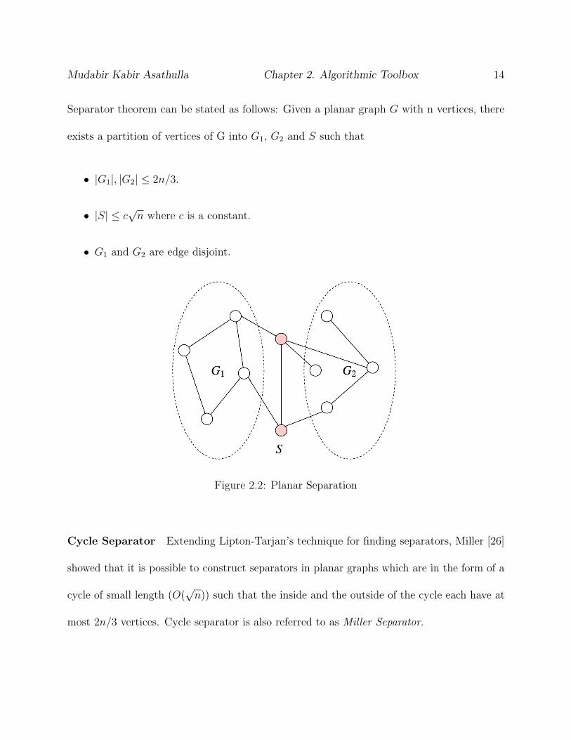
Separator theorem can be stated as follows: Given a planar graph G with n vertices, there

exists a partition of vertices of G into G1, G2 and S such that

• |G1|, |G2| ≤ 2n/3.

• |S| ≤ c√n where c is a constant.

• G1 and G2 are edge disjoint.

Figure 2.2: Planar Separation

Cycle Separator Extending Lipton-Tarjan’s technique for finding separators, Miller [26]

showed that it is possible to construct separators in planar graphs which are in the form of a

cycle of small length (O(√n)) such that the inside and the outside of the cycle each have at

most 2n/3 vertices. Cycle separator is also referred to as Miller Separator.


2.3 Lipton-Tarjan Divide and Conquer Algorithm

As one of many applications of planar separator theorem [24], Lipton and Tarjan showed

that maximum cardinality matching problem in planar graphs can be solved efficiently in

a divide and conquer fashion using planar separators. A planar separator can be used to

subdivide the matching problem into two sub-problems, each of size at most 2n3

. Maximum

matching in each sub-problem is computed using a divide and conquer approach. When the

sub-problem size becomes a small constant, we use Ford-Fulkerson algorithm to solve the

sub-problem. Given the maximum matching for two sub-problems, the maximum matching

for the current problem is computed in the merge step by introducing the boundary vertices.

For ease of explanation, we will consider the merge step at the top most level of divide and

conquer decomposition throughout this document in all chapters, unless stated otherwise.

The same description for merge operation can be carried over to any sub-graph in the divide

and conquer tree. The recurrence relation for this divide and conquer algorithm can be

written as

T (n) = T (αn) + T ((1− α)n) + g(n)

where 13≤ α ≤ 2

3and g(n) is the merge time.

Consider a bipartite graph G(A ∪B,E) divided by planar separators into sub-graphs X

and Y by removal of a set of boundary vertices, S. Before the merge step, we recursively

find a maximum matching in X and Y which imply that the residual graphs XM and YM


have no augmenting paths. During the merge step, we compute a maximum matching M∗

in G. The symmetric difference of the current matching M(X) ∪M(Y ) with the maximum

matching M∗ gives us a set of vertex-disjoint augmenting paths each passing through at least

one vertex in S. This implies that |M∗| − (|M(X)|+ |M(Y )|) ≤ |S| or in other words, the

number of remaining augmenting paths in G is O(√n).

Lemma 2. Number of augmenting paths remaining in G at the start of the merge step of

Lipton-Tarjan Divide and Conquer algorithm is O(√n).

Lipton and Tarjan showed that using Ford-Fulkerson algorithm to find one augmenting

path at a time in merge step gives g(n) = O(n3/2). The overall complexity of the recurrence

relation above is dominated by merge time when g(n) is∼O(nc) where c > 1. In such a case, the

complexity of the algorithm is given by g(n). Thus the overall complexity of Lipton-Tarjan

algorithm for maximum cardinality matching is O(n3/2).

2.4 r-division of Planar Graphs

Frederickson [10] showed that the planar separator theorem of Lipton and Tarjan [23] can

be used to obtain an r-division of a planar graph G with n vertices, which is the division of G

into O(n/r) edge disjoint sub-graphs called regions, each with O(r) vertices and O(r) edges.

Let {R1(V1, E1), ..., Rl(Vl, El)} be the disjoint regions obtained by r-division of G(A∪B,E)

where l is O(n/r). A vertex which is shared among two or more regions is a boundary vertex.


For a partition Rj, let Kj denote its set of boundary vertices. A vertex that belongs to just

one region is called an internal vertex of that region. The division ensures that every edge of

G is in exactly one region Rj. Specifically, the r-division {R1(V1, E1), ..., Rl(Vl, El)} has the

following properties:

•⋃

j Vj = A ∪ B and Ej = {(a, b) | (a, b) ∈ E, a, b ∈ Vj}. If vertices a, b are common

boundary vertices in multiple regions, include the edge (a, b) in only one of the regions.

• |Vj| = O(r) and |Kj| = O(√r)

• There are O(n/r) partitions and O(n/√r) boundary vertices after r-division of G.

• All boundary vertices in a region Rj lie in constant number of faces in planar embedding

of Rj (also called holes)

Like most algorithms which require cyclic ordering of boundary vertices in each region,

we use Miller’s cycle separator theorem [26] for the recursive decomposition (r-division).

Fakcharoenphol and Rao [9] presented an O(n log n) time recursive decomposition using

Miller’s separator where each region has a constant number of holes. Holes of a region R

are the bounded faces of R introduced by the cycle separators and are not faces of original

graph G. Constant number of holes in each region is a necessity for our∼O(n5/4) and

∼O(n6/5)

algorithm as we will see in Chapter 4. Our∼O(n4/3) algorithm is however immune to number

of holes in each region.


2.5 Dense Distance Graphs

We use dense distance graph to answer connectivity queries between boundary vertices of

a region (piece of r-division) for construction of edges of H. We maintain one DDG (Dj) for

each region (Rj) of a r-division of G. The union⋃

j Dj is called the DDG of entire graph G

(with respect to that r-division).

Dj contains only the boundary vertices of Rj. Dj includes a directed edge from one

boundary vertex u to another boundary vertex v in Rj if there is a directed path from u to v

through edges within RMj (residual graph of Rj). The edge also carries a weight representing

the shortest path length from u to v within RMj . Since there are O(r) pairs of boundary

vertices in Dj, it could have O(r) edges. We can ignore the edge weights if we are only

interested in the connectivity.

Before we go into the details of construction of DDG, we introduce the Monge property

in Section 2.5.1 which is satisfied by all shortest length paths between boundary vertices

in planar graphs. We provide high-level details of decomposition of DDG into bipartite

Monge groups and the operations that can be performed on these groups using an associated

data structures called Monge heaps. We also give an overview of implementing Dijkstra’s

algorithm using Monge heaps (FR-Dijkstra) that is in turn used to construct DDGs in divide

and conquer fashion. For detailed analysis, refer [9], [19]. Some of the ideas in this section

are borrowed for faster implementations of BFS and DFS which are described in Chapter 4.


2.5.1 Monge property in Planar Graphs

Given ordered sets of boundary vertices X and Y , we can define Monge property for

shortest distances d between pairs of elements in X and Y as follows: The sum of the shortest

distances when the pairs do not cross is at most the sum when the pairs cross. Consider

Figure 2.3: Monge Crossing property for distances

Figure 2.3 where u, v ∈ X, and x, y ∈ Y , order wise u ≤ v and x ≤ y, then

d(u, x) + d(v, y) ≤ d(u, y) + d(v, x)

. As a direct consequence of this, we can see that the shortest paths do not cross in a

Bipartite group i.e. if d(v, x) ≤ d(u, x), then d(u, y) has to be greater than or equal to d(v, y)

to satisfy the Monge inequality. Otherwise, we arrive at a contradiction (see Figure 2.3 (b)).

Since the paths from v → x and u→ x intersect at w and d(v, x) is shorter than d(u, x) by


our assumption, it also implies that v → w is shorter than u → w. Thus, it is clear that

d(v, y) ≤ d(u, y) if d(v, x) ≤ d(u, x). This is also called the non-crossing property.

2.5.2 Bipartite Monge Groups

To perform Dijkstra faster, the dense distance graph is decomposed into bipartite graphs.

We know that in any dense distance graph, we can ensure that the boundary vertices lie

in constant number of faces (holes) and have a cyclic ordering in the face they belong to.

For the sake of simplicity, we will consider that the boundary vertices are in only one face

and we can find a planar embedding such that the face becomes the infinite face. (Refer

section 5 of [9] for handling constant number of holes). We split the boundary vertices into

approximately two equal halves X and Y creating a complete bipartite graph on X and Y

with edges going from X to Y . Using the same vertices, we define another bipartite graph

with edges going from Y to X. The edges in the bipartite graph obey the Monge property

i.e. the shortest paths do not cross. Therefore, every vertex x in X has a contiguous interval

of vertices in Y , say Ix which have the shortest distance from x amongst all the vertices in

X. We continue dividing X and Y into almost equal halves successively (see Figure 2.4) and

end up with at most O(k) bipartite groups for the piece, k being the number of boundary

vertices in the piece. For a region Rj obtained from r-division, where k is O(√r), we have

O(√r) bipartite Monge graphs with each boundary vertex in at most O(log r) groups and

each edge in exactly one of the groups.


Figure 2.4: Successive Bipartite Monge Decomposition

We maintain a data structure for each Monge group which we call the Monge heap. We

will use (X, Y ) to represent both bipartite Monge group and Monge heap depending on the

context used and where differentiation is needed, we use M(X, Y ) to represent Monge heaps.

The nodes on the left of Monge group have labels associated with them and the label of a

vertex v on the right is given by δ(v) = minu∈X{δ(u) + w(u, v)} where w(u, v) is the weight

of the edge from u to v in the DDG which is also the shortest path from u to v in the region

Rj corresponding to the DDG that the Monge array is part of. When there is no edge from

vertex u to v in DDG, it implies that there is no path from u to v in the the corresponding

region of the original graph. In the Monge groups, we add an infinite weight edge from u to

v when there is no path from u to v. Therefore, the bipartite Monge groups are complete on

the node set X ∪ Y .

Online bipartite Monge Search Before diving into FR-Dijkstra, we describe this im-

portant subroutine of FR-Dijkstra on DDGs. In every Monge groups, we maintain a set of


active nodes A∗ ⊆ X, representing the frontier of Dijkstra search and set of matched nodes

M ⊆ Y representing nodes whose Dijkstra shortest path parent has been discovered. Each

Monge heap supports three operations.

• FINDMIN: Returns minimum unmatched node y ∈ Y \M from the heap. (O(1) time)

• EXTRACTMIN: Adds the current minimum y to M . For its parent x ∈ A∗, the interval

[i−(x), i+(x)] containing y is split into [i−(x), y) and (y, i+(x)] and the shortest edges

(found using Least Common Ancestor/Range Minimum Query data structure) in these

intervals are added to the heap. Instead of maintaining multiple intervals per vertex

x ∈ X, whenever we split intervals, we can also replace x with two dummy nodes x′

and x′′. One extra node is created in X whenever a node in Y is matched. This entire

operation runs in O(log (|X|+ |Y |) time.

• ACTIVATE(xi,δ(xi)): xi is activated in all the bipartite groups where it occurs on X

(left-hand side). Its interval in Y , Ixiis computed and other intervals are adjusted and

the heap is updated. If the vertex xi is first to be activated in the group, its interval is

whole of Y . Otherwise, walk up in A∗ until first xk whose d(xk, i−(xk)) < d(xi, i−(xk)).

Do a binary search for i−(xi) in the range [i−(xk), i+(xk)). Similarly, i+(xi) can be

found by walking down in A∗. After computing Ixi, for nodes between xi and xk, all

their intervals become empty and their corresponding min in Y \M are removed from

the heap. Do the same for nodes whose intervals are affected by walking down. New

min for xk and for the corresponding node while walking down are updated in the heap.


Figure 2.5: Intervals before and after vertex x8 is activated

ACTIVATE has an amortized run time O(log (|X|+ |Y |) per operation. Figure 2.5

illustrates interval adjustment when vertex x8 is activated. Note that y3 and y9 are not

in any intervals implying that they have already been matched.

2.5.3 Efficient Dijkstra Search in Dense Distance Graphs

FR- Dijkstra is an efficient Dijkstra implementation on Dense distance graphs due to

Fackcharoenphol and Rao. FR-Dijkstra algorithm constructs a single source shortest path

tree on the vertices of the DDG (boundary vertices of the original graph) with some boundary


vertex as source in time proportional to number of vertices in DDG while the traditional

Dijkstra algorithm runs in time proportional to the number of edges in the DDG.

By combining DDGs of all regions of r-division, we can perform FR-Dijkstra on the

boundary vertices of the entire graph. The run time is proportional to O(n/√r) (the total

number of boundary vertices) instead of O(n) which is the number of edges between boundary

vertices across all DDGs.

Each DDG is decomposed into bipartite monge groups. In addition to a heap for each

bipartite group, FR-Dijkstra algorithm uses a global heap Q having vertices with smallest

labels from each bipartite Monge group instance (Xi, Yi). In each iteration, a vertex v having

smallest label in Q is extracted and the Monge heap (X, Y ) that contributed v updates its

new smallest vertex to the global heap Q after adding v to M . Since a vertex can be in

O(log r) bipartite groups in every region of r-division that it is part of, it may be extracted

from Q multiple times with different labels from different local Monge heaps belonging to

different regions. However, its Dijkstra distance is fixed the first time it is extracted. After

a vertex v is extracted for the first time, it is added to the Dijkstra search frontier using

ACTIVATE which adds v to A∗ and updates all the Monge heaps containing vertex v in X

and their representatives in Q.

Run time of FR-Dijkstra is bounded by the number of calls to FINDMIN, EXTRACTMIN

and ACTIVATE. EXTRACTMIN and ACTIVATE are called at most once per vertex in


each Monge heap and FINDMIN is called whenever EXTRACTMIN or ACTIVATE is called.

In region Rj, its DDG (Dj) has each boundary vertex appearing in O(log r) Monge heaps

and this bounds the total number of operations to O(√r log r) per region. Each operation

takes at most O(log r). Therefore FR-Dijkstra takes O(√r log2 r) time per region Rj or

O((n/√r) log2 n) time in the entire graph.

We use FR-Dijkstra with slight changes to do BFS on compressed residual graph H in

Chapter 4. Theoretically, BFS is just Dijkstra’s algorithm with unit edge costs. We reserve

the pseudo code for Chapter 4. We also modify FR-Dijkstra to do FastDFS on H in Chapter

4.

2.5.4 Construction of DDG

Dense distance graph Dj of a region Rj is constructed in a divide and conquer approach.

The sub-graph Rj is recursively divided into smaller pieces using cyclic planar separators

forming a decomposition tree. A boundary vertex in level i of decomposition is also a

boundary vertex in level i+ 1 sub-piece. In addition to that, decomposition of level i piece

to form level i + 1 sub-pieces can introduce new boundary vertices in each of the level

i + 1 sub-pieces. The dense distance graph for the parent at level i of decomposition is

constructed from the dense distance graphs of its children at level i + 1. This is possible

through FR-Dijkstra routine which runs in time proportional to number of boundary vertices

in both the children which is O(√v) more the number of boundary vertices in the parent, v


being the number of vertices in the parent. Fakcharoenphol and Rao [cf section 5, [9]] also

proposed a 3-level decomposition which ensures an exponential decrease in number of total

vertices and boundary vertices for every 3 levels of decomposition and restricts the count of

holes in every piece of decomposition tree to not exceed a constant value.

Computing the shortest path tree from each boundary vertex using FR-Dijkstra takes

O(√r log2 r) time. We invoke FR-Dijkstra for all boundary vertices. Therefore the total time

taken for all Dijkstra computations is O(√r√r log2 r) = O(r log2 r). Since there are O(log r)

levels in the recursive decomposition, the overall time to compute dense distance graph per

region takes time O(r log3 r). The query time to check for connectivity from vertex u →

v takes O(log r) time. Data structures with better construction time and query time exist

for creation of dense distance graph to answer connectivity queries. Klein’s multiple source

shortest path data structure [21] has a construction time of O(r log r) per region and query

time of O(log r). Thorup’s data structure [29] has a O(r log r) construction time and can

answer connectivity queries in constant time.

Chapter 3

New Matching Algorithm

Our algorithm adapts Lipton-Tarjan’s divide and conquer technique as described in Section

2.3. We improve the merge time g(n) from O(n3/2) to O(n6/5 log2 n) by exploiting planar graph

properties. We first present the details of a simpler version of our merge algorithm which has a

run time of∼O(n4/3). We also provide proof of correctness and run-time analysis. We conclude

this chapter by stating the similarity between our merge algorithm and Hopcroft-Karp

algorithm.

Algorithm Organization We begin by describing two operations that are performed at

the beginning of our merge algorithm namely

• Preprocessing (Section 3.2)

• Construction of Compressed Residual Graph H (Section 3.3)

27

Mudabir Kabir Asathulla Chapter 3. New Matching Algorithm 28

We then perform a Hopcroft-Karp style algorithm on H to compute maximum matching

in G. The details of the Hopcroft-Karp style algorithm is provided in Section 3.5.

3.1 Convention for Notation

We are given a bipartite graph G. We refer to its residual graph as GM . The vertex and edge

sets of G and GM are identical (except for the directions) and a matching, alternating path

or an alternating cycle in G is also a matching, alternating path or an alternating cycle in

GM . If P is a subset of edges in G, we will also use P to denote the same subset of edges in

GM , the directions of the edges being determined by whether or not an edge is in M . We

know that r-division partitions the edges of G into regions⋃

j Rj. Since G and GM have the

same underlying set of edges, we use Rj to also represent regions of GM . Dense distance

graph Dj corresponding to each region Rj is constructed from boundary vertices of Rj. We

use Kj to represent boundary vertices of both Rj and Dj.

H is a compressed residual graph that we construct using the r-division boundary vertices

of GM (details in Section 3.3) and the unmatched internal vertices in each region of GM . We

use the boundary vertices of GM to define regions⋃

j RHj in H and just like in Dj, we also

use Kj to represent boundary vertices of region RHj in H. The compressed residual graph

changes whenever GM changes. For convenience, we will still use a single notation H to

represent the changing compressed residual graph. We also state explicitly whether we are


referring to the compressed residual graph before or after the change to avoid confusion for

readers.

3.2 Preprocessing

There are at most O(√n) augmenting paths remaining at the beginning of merge step

(Lemma 2). We find r-division of G(A ∪B,E). In each region (Rj) of G after r-division, we

do DFS iteratively from unmatched vertices of type B to find augmenting paths lying wholly

within Rj. An unmatched vertex can be an internal vertex or a boundary vertex.

Each DFS takes O(r) time. We need to do at most O(√n) iterations of DFS in total from

unmatched internal vertices as there cannot be more than O(√n) unmatched internal vertices

at the beginning of merge step. Thus the total time taken to do DFS from unmatched internal

vertices is O(√nr). Since the total number of boundary vertices in each region Rj of graph

G after r-division is O(√r) and there is O(n/r) regions, we can bound the total number

of iterations of DFS from unmatched boundary vertices to be O(n/√r). Even though a

boundary vertex can belong to multiple regions, it can have a matching in at most one region.

Once a boundary vertex is matched in a region, we need not repeat DFS from this vertex

in the remaining regions that contain it. The total time taken to do DFS from unmatched

boundary vertices across all regions is O(n√r). For any r < n, n

√r >

√nr. Thus the

preprocessing step has O(n√r) run time.


Preprocessing step ensures that augmenting paths within each region are eliminated and

the remaining augmenting paths must span multiple regions. In other words, the remaining

augmenting paths in GM should include at least one matched boundary vertex.

Lemma 3. After the preprocessing step, there are O(√n) augmenting paths remaining in

GM and there is no augmenting path which lies wholly inside a region Rj.

3.3 Compressed Residual Graph H

Given a current matching M after the preprocessing step, the sparse graph H is a multi-

graph constructed on the boundary vertices and free vertices of A ∪ B. Let AF and BF

denote the set of free vertices of A and B respectively after finding maximum matching in

each region. The vertex set of H, denoted by VH , will contain all the boundary vertices i.e.,

∪lj=1Kj. Therefore, every free vertex that is also a boundary vertex will automatically be in

VH . For every partition Rj(Vj, Ej), if at least one free vertex from AF ∩ Vj is not a boundary

vertex, i.e., (Vj\Kj) ∩ AF 6= ∅, a special vertex aj is added in VH to represent all the free

vertices of (Vj\Kj) ∩ AF . Similarly, vertex bj is added in VH for the set of free vertices of

(Vj\Kj) ∩BF . We call these additional vertices of VH , aj and bj, free internal vertices. The

vertex set VH of H is thus given by VH =⋃l

j=1(Kj ∪ {aj, bj}). The nodes of H are classified

depending on whether they are from A or B as follows: AH =⋃

j((Kj ∩ A) ∪ {aj}) and

BH =⋃

j((Kj ∩ B) ∪ {bj}). Clearly, VH = AH ∪ BH . We refer to AFH = (AH ∩ AF )∪

⋃j aj

and BFH = (BH ∩BF )∪

⋃j bj as the free vertices of AH and BH .


After defining the vertex set VH of H, edges between these vertices are constructed as

follows. In order to define the edge set of H, we consider the residual graph GM after

preprocessing where we find maximum matching in each region of the r-division. Let Mj be

the edges of the matching M that are contained in Rj, i.e., Mj = M ∩ Ej. The edges in H

are of three types.

• u, v ∈ Kj are both boundary vertices and there is a directed path from u to v in GM

that only passes through the edges of Rj. Note that H is a multi-graph in general

because of edges of this type; multiple regions can contribute to edges between same

pairs of boundary vertices.

• u = bj and v ∈ Kj, and there is a directed path in GM from some free vertex in

BF ∩ (Vj\Kj) to v that only passes through the edges of Rj.

• u ∈ Kj and v = aj, and there is a directed path in GM from u to a vertex v in the set

AF ∩ (Vj\Kj) that only passes through the edges of Rj.

We will denote by EHj , the set of edges in H between vertices u, v ∈ (Kj ∪ {aj, bj}). For

every edge (u, v) ∈ EHj , the projection of the edge (u, v) on the residual graph GM is the

corresponding shortest directed path from u and v in GM using only edges of Rj. This can

be obtained by doing a BFS from u in Rj.

Lemma 4. H has O(n/√r) vertices and O(n) edges.

Proof. The vertex set of H consists of free internal vertices and set of boundary vertices. At


most two free internal vertices are added per region. Since there are O(n/r) partitions, total

number of free internal vertices is O(n/r). On the other hand, there are O(√r) boundary

vertices in each region in H. Therefore the total number of boundary vertices in H can be

bounded by O(n/r) ∗O(√r) = O(n/

√r). This also bounds the total number of vertices in H.

In each region, every pair of boundary vertices may have an induced edge between them.

Therefore there are O(r) such edges per region. There are at most O(√r) edges per region

where one end vertex is a free internal vertex. So, the bound on total number of edges in a

region is O(r). Since there are O(n/r) partitions, the total number of edges in all the regions

of H is O(n). �

For computing H, we construct a dense distance graph for each region as described by

Fakcharoenphol and Rao [9]. We covered dense distance graphs in section 2.5. The dense

distance graph stores all-pairs shortest path distances between boundary vertices in the

region.

Let RHj be a sub-graph in H with vertex set (Kj ∪ {aj, bj}) and edge set EH

j . We refer to

RH1 , R

H2 . . . R

Hl as regions of H. Connectivity between each pair of boundary vertices in the

region can be established in O(log r) time after construction of dense distance graph and

there are O(r) combinations of pairs of boundary vertices. To compute edges of the type

(u, v) ∈ bj ×Kj , we add an additional vertex b to the subset of the residual graph GM defined

by matching Mj in Rj and add an edge from b to every vertex in (BF ∩ Vj)\Kj. Next, we


execute BFS from b in the subset of residual graph GM in the region Rj and include the edge

(u, v) in RHj only if there is path to v from b in the BFS search. BFS takes O(r) time as the

number of edges is O(r) in RMj . Using a similar approach with the edges of GM reversed and

a newly added vertex a in Rj , we compute edges of the type (u, v) ∈ Kj × aj . This yields the

following Lemma:

Lemma 5. The edges of H in any partition RHj can be computed in O(r log r) time.

Proof. While constructing H, we also store information on immediate neighbors of each

vertex. In each region RHj , for every vertex u in the region, we maintain an adjacency list of

all vertices that it has edges to, which we refer to as neighbors of u in RHj . With a constant

number of holes (say h) in each region, instead of maintaining a single neighbors list for

each vertex, we need to maintain h lists of neighbors for each vertex, one each for neighbor

vertices lying on a particular face. Each boundary vertex u also has separate list for edges of

type (u, aj). Since a boundary vertex belongs to multiple regions, it will have one or more

neighbors lists for each region it belongs to depending on the number of holes in that region.

Moreover, boundary vertices have a cyclic order in their respective face (hole). Therefore, for

each vertex, the neighbors list corresponding to each hole has vertices stored in cyclic order.

For the sake of simplicity, for the rest of chapter 3 and for chapter 4, we will assume that all

boundary vertices lie on the infinite face and for each vertex u in a region, there is only one

neighbors list in that region denoted by N(u,RHj ) comprising of just boundary vertices which

are neighbors of u. u also maintains a separate list for edges of type (u, aj) as mentioned

before. All descriptions henceforth will make this assumption and can be easily carried over


to the handle constant number of holes as well. �

Definition 3.3.1. We define Augmenting path in H as a simple directed path (no cycles) in

H from a free vertex in BFH to a free vertex in AF

H .

3.4 Projection and Lifting

Up until now, we have described the creation of the compressed graph H. Before diving

into our algorithm, we introduce two operations involving G and H, namely projection and

lifting.

3.4.1 Projecting a path.

To project a path P ′ in the compressed residual graph H to a path P in residual graph GM ,

each edge (u, v) of P ′ is to be replaced by some directed path between the end vertices u

and v in GM . Edges (u, v) of type u, v ∈ Kj can be projected to G by querying the dense

distance graph Dj which returns the shortest path between u and v. An edge (u, v) of type

u = bj, v ∈ Kj (or u ∈ Kj, v = aj) can be projected to G in just the same way they were

constructed by doing BFS from b (or a) and identifying a free vertex in (Vj\Kj) ∩ BF (or

(Vj\Kj) ∩ AF ) that has a path to (or from) the boundary vertex.


Figure 3.1: A path in GM is lifted to H. An edge in H is projected to shortest path in GM .

3.4.2 Lifting a path.

Consider a directed path P in GM . Among the vertices of P , let pi1 , pi2 , . . . , pil with

i1 < i2 < i3 < . . . < il, be all its boundary vertices. Let Pit be the sub-path of P lying

between the vertices pit and pit+1 . Note that Pi0 will be the sub-path in P appearing before

the vertex pi1 and Pil is the sub-path in P appearing after the vertex vil . Also, note that if

pit and pit+1 are adjacent to each other in P , then Pit will contain only one edge, i.e., the

edge with pit and pit+1 as endpoints. We will map any sub-path Pit with u and u′ as its first

and last vertex to an edge (v, v′) in H. This edge (v, v′) is referred to as the lift of the path

Pit and is constructed as follows. Note that if both u and u′ are boundary vertices, we set

v ← u and v′ ← u′. Suppose, u is a free internal vertex of B in partition Rj . In this case, we

set u to bj. A similar construction is applied in the case where u′ is a free internal vertex of

A. Let e′it be the lift of the path Pit . It is easy to see that the path < e′i0 , e′i1, e′i2 , . . . , e

′il> is

a path in H. We say that this path P ′ in H is obtained by lifting the path P to H. As a


consequence of the lifting operation, we get the following corollary.

Corollary 1. If the matching M is not a maximum matching in G, then there is an augmenting

path in H.

Proof. Let M∗ be optimal matching in G. M∗ ⊕M gives a set of vertex disjoint augmenting

paths in GM . Any augmenting path in GM starting at u ∈ BF and ending at u′ ∈ AF is

lifted to a path in H beginning at v ∈ BFH and ending at VH ∈ AF

H by above construction of

lifting which also happens to be an augmenting path in H by definition. �

Lemma 6. Let P1 and P2 be two vertex-disjoint directed paths in GM and Q1 and Q2 be the

paths obtained by lifting them to the graph H. Let Q′1 (resp Q′2) be all the vertices on the path

Q1(resp Q2) except for its start and end vertex, then

Q′1 ∩Q′2 = ∅

Proof. This is again a consequence of lifting operation. Since paths P1 and P2 are vertex

disjoint in GM , it also implies that they share no common boundary vertices between them.

When these paths are lifted to H, Q1 and Q2 will also have a disjoint set of boundary vertices.

A path in H comprises of just the boundary vertices except for possibly the start and the end

vertex which could of type bj and aj respectively. By discarding the first and last vertex from

Q1 and Q2, the intermediate vertices are only boundary vertices. Thus we get Q′1 ∩Q′2 = ∅.

�


Figure 3.2: Vertex disjoint paths in G (shown in red) have disjoint boundary vertices in H

3.5 Merge Algorithm

After performing the preprocessing (Section 3.2) and construction of H (Section 3.3), we

execute a Hopcroft-Karp style algorithm on H to compute maximum matching in G. We will

show in Section 3.7 that this improves the merge time of our divide and conquer algorithm.

Our algorithm runs in phases till we have a maximum/perfect matching in G. In each

phase, we do the following steps.


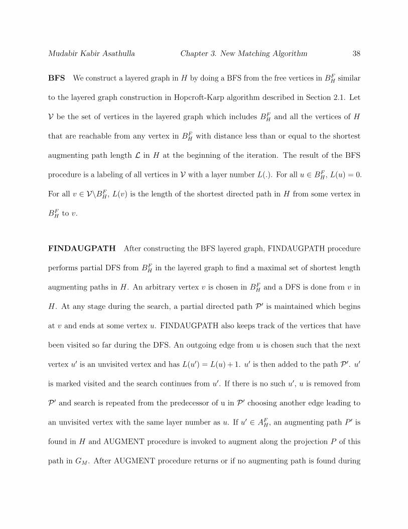
BFS We construct a layered graph in H by doing a BFS from the free vertices in BFH similar

to the layered graph construction in Hopcroft-Karp algorithm described in Section 2.1. Let

V be the set of vertices in the layered graph which includes BFH and all the vertices of H

that are reachable from any vertex in BFH with distance less than or equal to the shortest

augmenting path length L in H at the beginning of the iteration. The result of the BFS

procedure is a labeling of all vertices in V with a layer number L(.). For all u ∈ BFH , L(u) = 0.

For all v ∈ V\BFH , L(v) is the length of the shortest directed path in H from some vertex in

BFH to v.

FINDAUGPATH After constructing the BFS layered graph, FINDAUGPATH procedure

performs partial DFS from BFH in the layered graph to find a maximal set of shortest length

augmenting paths in H. An arbitrary vertex v is chosen in BFH and a DFS is done from v in

H. At any stage during the search, a partial directed path P ′ is maintained which begins

at v and ends at some vertex u. FINDAUGPATH also keeps track of the vertices that have

been visited so far during the DFS. An outgoing edge from u is chosen such that the next

vertex u′ is an unvisited vertex and has L(u′) = L(u) + 1. u′ is then added to the path P ′. u′

is marked visited and the search continues from u′. If there is no such u′, u is removed from

P ′ and search is repeated from the predecessor of u in P ′ choosing another edge leading to

an unvisited vertex with the same layer number as u. If u′ ∈ AFH , an augmenting path P ′ is

found in H and AUGMENT procedure is invoked to augment along the projection P of this

path in GM . After AUGMENT procedure returns or if no augmenting path is found during


DFS from v , FINDAUGPATH initiates a new search from the next unvisited vertex in BFH .

AUGMENT The AUGMENT procedure takes as input, an augmenting path P ′ in H. We

denote a partition Rj of G as affected if the path P ′ has at least one edge from the edges of H

in EHj . Let R be the set of all affected partitions. Each directed edge (u, v) in P ′ belonging

to EHj is projected in the corresponding region Rj . Let P be the projection of P ′ on GM . By

rules of projection, P also starts and ends in a unmatched vertex. We will show in Lemma

16 that P is a simple path and contains no self-intersections. Therefore, P is an augmenting

path in GM . After augmenting along P , the residual graph GM changes and the edges in

each partition in R are recomputed in H. Reconstruction can be done in each region using

the same data structures that we used to construct H in Section 3.3.

In each phase of our Hopcroft-Karp style algorithm, FINDAUGPATH finds a maximal

set of shortest length augmenting paths in H (Lemma 15) which are also boundary vertex

disjoint (Lemma 14). Unlike the Hopcroft-Karp algorithm, we augment in GM immediately

after finding an augmenting path during partial DFS in H. Since H changes (only affected

regions) after each augmentation, the new compressed residual graph H may introduce new

augmenting paths. We show in Lemma 12 that all such augmenting paths are of length ≥ L

which is the length of the shortest augmenting path in the beginning of the phase. Also,

since H changes after each augmentation, it may affect the layer numbers of some vertices in

H. For this reason, it may seem necessary to perform BFS again to construct new layered

graph after each augmentation. We, however show that it suffices to do BFS just once at the


beginning of each phase (Lemma 11, 12, 14) and that vertices whose layer numbers change

will not be part of shortest length augmenting path in the current phase. We also show that

the length of the shortest augmenting paths in H increases (Lemma 15) after each phase

of our algorithm and the number of iterations required to compute maximum matching is

O(√VH) (Lemma 17).

Our algorithm maintains the following invariant.

(I1) Projection P of an augmenting path P ′ in H onto GM is a simple path i.e., the path P

does not have any self-intersections.

3.6 Proof of Correctness

In this section, we state and prove some properties to justify the correctness of our

Hopcroft-Karp style algorithm.

We assume the invariant (I1) for proving lemmas 11 to 15. We later prove the invariant

(I1) in Lemma 16.

Definition 3.6.1. An edge (u, v) in H is called level respecting if L(v) ≤ L(u) + 1 and the

edge is said to be in the level L(u) .

L(.) refers to layer numbers assigned to vertices by the BFS procedure of our Hopcroft-Karp


style algorithm. Before finding the augmenting paths in H, all the edges in H between

vertices in layered graph are level respecting.

Lemma 7. Two level respecting edges (u, v) and (u′, v′) in H lying in the same region RHj

and satisfying the following conditions

1. L(v) = L(u) + 1, L(v′) = L(u′) + 1

2. L(u′) ≥ L(u) + 1

will always have vertex-disjoint projections.

Proof. Consider two level respecting edges (u, v) and (u′, v′) in region RHj satisfying the above

2 conditions. From the two conditions, we can infer L(v′) ≥ L(u) + 2. Let us assume that

the projections of (u, v) and (u′, v′) share a common vertex w. This would mean that u has

a path to v′ through w in GM and by rules of construction of H, there should be an edge

(u, v′) in H assigning L(v′) = L(u) + 1. Thus, we arrive at a contradiction. �

Reversing some edges in the region Rj of GM can create and destroy edges in the region

RHj of H while all other regions of H remain unaffected. In Lemmas 8 to 11, we state and

prove some properties that are obeyed by new edges introduced in H due to changes in the

residual graph GM .

Definition 3.6.2. A directed path from vertex u to v in GM (or H) is of shortest length if

the path uses minimum number of edges among all the paths from u to v in GM (or H).


Lemma 8. If the projection of an edge (u, v) with L(v) = L(u) + 1 is reversed in GM , the

new edges created in H will be level respecting and will have a level greater than or equal to

L(u).

Proof. After reversing the projection P of edge (u, v), new paths are introduced between

boundary vertices of Rj in GM that use one or more reversed edges of P . This could lead to

new edges being introduced in H and each of these edges have least one of the reversed edges

of P in their projection.

Let (u′, v′) be one of the newly formed edges in H. Projection of (u′, v′) uses at least one

of the reversed edges of P . Let w be the first common vertex which is both in projection of

(u′, v′) and in P . Before reversing the projection P , there was a directed path from w to v in

Rj along P . This implies that u′ also had a path through w to v before reversing P . Thus,

by construction of H, there must have been an edge (u′, v) in H before reversing P as shown

in the second diagram of Figure 3.3. Let L(u) = i and L(v) = i+ 1. Since the edge (u′, v) is

level respecting and L(v) = i+ 1, we can infer that L(u′) ≥ i.

After reversing P , u′ which had a path to v through w would now have a path to u through

w using the reversed edges of P . u′ will also have a path to all neighbors of u after reversal

of P . Thus v′ in the newly edge could either be u or a neighbor of u in RHj after reversal of

P . If v′ is a neighbor of u, (u, v′) must have existed even before reversing P . (u, v′) is also

level respecting and therefore L(v′) ≤ i + 1. If v′ is u, it would still satisfy the condition


L(v′) ≤ i+ 1 as L(u) = i. Since L(u′) ≥ i and L(v′) ≤ i+ 1, we can conclude that the newly

added edge (u′, v′) also satisfies the definition of level respecting. Moreover, the newly added

Figure 3.3: L(u) and L(v′) can only increase or remain same after augmentation.

edge will have level greater than or equal to i since L(w) ≥ i. �

Lemma 9. Reversing the projection of an edge (u, v) ∈ RHj where L(v) = L(u) + 1 does not

create or destroy a level respecting edge with level < L(u) in RHj .

Proof. We showed in Lemma 8 that reversing the projection of (u, v) only introduces level

respecting edges in H. We also showed that these edges are at level ≥ L(u) in RHj . We now

show that no level respecting edge with level < L(u) is destroyed by reversing the projection

of (u, v).

Projection of any level respecting edge (u′, v′) at level < i will only have vertices with

L(.) ≤ i and it should also be vertex-disjoint (hence also edge-disjoint) from the projection

of (u, v). Otherwise, u′ would have a path to v in Rj through the common vertex of two


projections and the corresponding edge (u′, v) in H would violate level respecting property.

This contradicts the fact that all edges in H are level respecting. Thus reversing the projection

of (u, v) does not remove any level respecting edge at level < i. �

Using Lemmas 11 to 14, we will show that the boundary vertices which are visited by the

FINGAUGPATH can be discarded as they will never be part of a newly found augmenting

path in the same phase of the algorithm.

After finding an augmenting path P ′ in H, its projection on GM , P is augmented, causing

each of its edges to get reversed in GM . When the path corresponding to projection of an

edge in P ′ gets reversed, it can lead to new edges being created between the vertices in H in

the region affected, which can affect the layer numbers of many vertices that were computed

by the BFS procedure.

Lemma 10. The new edges introduced in H after augmenting the projection of P ′ in G

satisfy the level respecting property.

Proof. We know that reversing the projection of an edge in RHj does not affect edges of H

in other regions. We also saw in Lemma 9 that reversing the projection of an edge (u, v) in

RHj where L(v) = L(u) + 1 does not affect the level respecting edges at lower levels. Since

reversing the projection of an edge in P ′ does not affect the edges of H in other regions and

in the lower levels of the same region, we can consider the effect of augmenting the path P

(projection of P ′) as being same as incrementally reversing the projection of edges in P ′, one


at a time from the end of the path AFH to the beginning BF

H .

After augmenting the projection of each edge in P ′, the newly created edges in H are also

level respecting as shown in Lemma 8. Extending this property to all the edges in P ′, we can

say that all the newly introduced edges in H after augmenting the path P would be level

respecting. �

Lemma 11. Layer number of vertices in H assigned by BFS step do not decrease after

augmenting a path P in G.

Proof. As shown in Lemma 10, all the newly added edges in H after augmenting the path P

in G are level respecting. Moreover, some of the edges which existed before augmentation

may be removed from H. Destroying an edge in H can only potentially increase the layer

number of vertices. Since all the newly created edges after augmentation are level respecting

with respect to the layer numbers L(.) computed by BFS at the beginning of the phase, the

newly formed edges do not create a shorter path to any vertex from BFH . Therefore, if we do

a BFS again from BFH to assign new layer numbers to vertices, the layer numbers would only

increase or remain the same.

�

Lemma 12. After augmenting along the projection of a path P ′ in H, the augmenting paths

in the new graph H after augmentation are of length ≥ |P ′|.

Proof. In Lemma 11, we showed that the layer numbers assigned by BFS to all vertices


including vertices in AFH can only increase or remain the same after augmenting along the

projection of path P ′. All vertices in AFH had layer number |P ′| before augmenting the

projection of P ′. After augmentation, using Lemma 11, we can infer that the length of

shortest path to vertices in AFH from any vertex in BF

H can only increase or remain same.

Thus all the remaining augmenting paths have length ≥ |P ′|. �

We showed in Lemma 11 that layer number of all vertices can only increase or remain the

same after augmentation. Using Lemma 14 and Lemma 13, we show that any vertex which is

visited by the FINDAUGPATH procedure in the current phase can be discarded and need

not be visited by FINDAUGPATH again. Lemma 13 shows why this is true for any vertex

which is visited but did not lead to a shortest length augmenting path. Lemma 14 shows that

we can also discard vertices which participated in an augmenting path in the current phase

as they will not be part of any other augmenting path of the shortest length discovered in

the same phase by FINDAUGPATH.

Let S(v) indicates the shortest path length from any vertex in BFH to v. At the beginning

of each phase, S(v) = L(v) which is assigned by BFS. If we construct a graph H ′ from H by

reversing all the edges in H and then do BFS on H ′ starting from AFH vertices at layer 0,

then we can make a similar argument that the shortest distance to any vertex v from AFH (or

shortest distance from v to AFH in H), denoted by S ′(v) increases or remains the same after

an augmentation.


The length of the shortest augmenting path through any vertex v can be represented as

sum of the length of shortest path of v from any vertex in BFH and the length of shortest

path from v to any vertex in AFH i.e. S(v) + S ′(v). Thus for any vertex v, if S(v) increases

after an augmentation, it will no longer be part of the shortest length augmenting path in

the current iteration. Its layer number also increases in the next phase. We have also shown

in Lemma 11 that S(v) can never decrease. This justifies the fact that it suffices to compute

BFS layers only once at the beginning of each phase and not after every augmentation. Only

those vertices whose S(.) = L(.) would be part of the shortest length augmenting paths in

the current phase.

Lemma 13. If a vertex is marked visited by FINGAUGPATH but did not lead to a shortest

length augmenting path, then it can not be part of any shortest length augmenting path

discovered later in the same phase.

Proof. Consider a vertex z which was explored in the current phase by FINDAUGPATH but

did not lead to a shortest length (|P ′|) augmenting path in the current phase. Let S(z) = i.

Since z was explored in the FINDAUGPATH and no augmenting path of length |P ′| was

found, it implies S ′(z) > (|P ′| − i). This implies that even if S(z) remains the same after

augmenting a path P ′, we still have S(z) + S ′(z) > |P ′|.

Alternatively, we can prove this by contradiction. Let us assume that vertex z was marked as

visited by FINDAUGPATH routine while doing a partial DFS from b1 ∈ BFH , but was not part

of a shortest length augmenting path. This implies S ′(z) > |P ′| − i. Later, FINDAUGPATH


Figure 3.4: If z is marked visited by partial DFS from b1, P1 is found before P2.

finds an augmenting path from b2 ∈ BFH to a ∈ AF

H through z which implies S ′(z) = |P ′| − i.

This leads to a contradiction as depicted in Figure 3.4. Since S ′(z) cannot reduce, the path

from z to a should have existed even during partial DFS from b1 and an augmenting path P1

would have been found the first time z was visited before P2 was discovered. This proves the

lemma. �

Lemma 14. No boundary vertex will be part of two or more augmenting paths of the same

length in H.

Proof. To prove this lemma, we will show that for a vertex v which is part of augmenting path

P ′, after augmenting along the projection of P ′, has at least one of S(v) or S ′(v) increasing

which means that the next shortest augmenting path through v will have a length > |P ′|.

The case where S(v) increases after augmenting P ′ is trivial as this implies that S(v)+S ′(v)

is now greater than |P ′|, the length of the shortest augmenting path in the current phase.


Let us consider the case where S(v) doesn’t change after an augmentation. In this case,

we will show that S ′(v) should increase. For the sake of contradiction, let us assume that

S ′(v) does not increase. Let (u, v) be the edge of the augmenting path P ′ which was just

augmented. Let the projection of (u, v) be {u, p1, p2, . . . , pl, v}. Let the new edge responsible

for maintaining the same layer number of v be (u′, v). This edge could be formed after

augmenting the projection of P ′ or may have existed before. If the edge (u′, v) existed before,

its projection after augmentation has to be edge-disjoint from the projection of (u, v) before

augmentation implying that v has 2 incoming edges in GM . If the edge (u′, v) was formed

after augmentation, its projection {u′, p′1, p′2, . . . , p′l, v} may use some of the reversed edges of

projection of (u, v) but the final edge (p′l, v) in projection of (u′, v) would still be different

from final edge (pl, v) in the projection of (u, v). In this case too, we can see that v has at

least 2 incoming edges in GM .

We know that in a bipartite matching, any vertex in B has at most 1 incoming edge and

every vertex in A has at most 1 outgoing edge in GM . Since vertex v has at least 2 incoming

edges in GM , it means v ∈ A and has only one outgoing edge in GM . v can have many

outgoing edges in H all of which share a common edge in their projections on GM . Reversing

the projection of any one of the outgoing edges from v in H during augmentation, invalidates

all other outgoing edges from v in H (See Figure 3.5). So, v can only have a path to a free

vertex in AFH through a vertex z which had layer number L(z) < L(v) before augmenting

the projection of P ′. Since S ′(z) > S ′(v), the second augmenting path through v has length


Figure 3.5: If S(u) remains same after augmentation, v has to be of type A.

> |P ′|. �

Lemma 15. Length of the shortest augmenting paths in H during the (i+ 1)th iteration is

at least 1 greater than the shortest augmenting path in ith iteration.

Proof. The shortest length of an augmenting path in H after running Hopcroft-Karp algorithm

in each region is at least 2. Let L be the length of the shortest augmenting path at the

beginning of a given phase. By Lemma 13 and 14, after augmenting a path of length L,

any remaining augmenting paths of the same length would use unvisited vertices except for

possibly the first and last vertices which could be internal vertices. We have also shown in

Lemma 12 that the length of any new augmenting path created in H after each augmentation

because of the newly added edges is greater than or equal to L. Lets say we do a partial


DFS from a free vertex b1 ∈ BFH and it did not lead to an augmenting path of length L. Our

algorithm continues to do partial DFS from the remaining free vertices in BFH . Lets assume

that a new augmenting path P ′′ of length L is created from b1 because of augmenting along

some augmenting path discovered later in the phase. Since our algorithm does not repeat

partial DFS from b1, P′′ may be missed which contradicts our lemma. However, we can show

that P ′′ cannot be created in the first place as it would mean S ′(b1) which was greater than

L initially has become equal to L which is not possible as we showed in Lemma 11 and 14.

Therefore, all augmenting paths of length L are exhaustively found in the given iteration.

The minimum length in the next iteration of merge algorithm is at least L+ 1. �

3.6.1 Proof of Invariant

While running the Hopcroft-Karp style algorithm on H, we maintain the following invariant.

Lemma 16. Let P ′ be an augmenting path reported by FINDAUGPATH and let P be its

projection on GM . Then P is a simple path.

Proof. By construction, P ′ is a simple path. For the sake of contradiction, let us assume that

there are at least two edges (u, v) and (u′, v′) in P ′ whose projections intersect. Without loss of

generality, let u′ come later in the path P ′. So, L(u′) ≥ L(u) + 1. Moreover, FINDAUGPATH

chooses edges such that L(v) = L(u) + 1 and L(v′) = L(u′) + 1. Let Puv and Pu′v′ be the

projections of the 2 edges. Since the projections intersect in GM , the projections are in the

same region Rj and share a common edge, say (w, x). This is because w cannot have multiple


Figure 3.6: Projection of 2 edges of augmenting path in H cannot intersect in G

incoming and multiple outgoing edges in a bipartite graph. This gives us the condition that

L(v′) ≥ L(u) + 3. Puv is a directed path from u to v through w in the region Rj of GM

and Pu′v′ is a directed path from u′ to v′ through w in the same region. This means that

there is also a directed path from u to v′ and by construction of H, there would have been

an edge from u to v′ in H. By BFS labeling, L(v′) ≤ L(u) + 1. This contradicts with our

earlier condition that L(v′) ≥ L(u) + 3. Therefore, our assumption that projections of 2

edges intersect is incorrect. Since no projections intersect, there cannot be a cycle in P and

it is a simple path. �


3.7 Algorithm Efficiency

Lemma 17. After√|VH | iterations of the algorithm, there will be at most O(

√|VH |) un-

matched nodes remaining.

Proof. From lemma 15, length of augmenting path in H grows by at least 1 after every

iteration. After√|VH | iterations, length of augmenting path in H is at least

√|VH |+ 2 with

at least (√|VH |) boundary vertices. Since we eliminated augmenting paths within each region

as part of preprocessing before running the Hopcroft-Karp style algorithm, the remaining

augmenting should span multiple regions. This implies that all augmenting paths in H

contain at least one boundary vertex.

We know that that symmetric difference of the optimal matching M∗ and the matching M

after√|VH | iterations will form a set of vertex-disjoint augmenting paths in GM . By Lemma

6, these paths map to paths in H which are vertex disjoint in H except for the first and

the last vertex. Thus the bound on vertex-disjoint augmenting paths in G can be found by

bounding vertex-disjoint augmenting paths in H excluding the first and last vertex. There

are O(VH) boundary vertices in total. From Lemma 15 and Lemma 6, the number of such

vertex-disjoint augmenting paths in H after (√VH) iterations is bound by O(VH)/(

√|VH |) =

O(√|VH |) thus proving the lemma. �


3.7.1 Efficiency of BFS, FINDAUGPATH and AUGMENT proce-

dures

The layered graph can be constructed with a single BFS in O(n) time. However, section

4.2 presents a way to accomplish this in O(|VH | log2 n) time, that is O( n√r

log2 n).

Let P ′i be the ith augmenting path in H computed by FINDAUGPATH procedure. For

an edge in P ′i belonging to RHj , computing its projection in GM using only the edges in Rj

takes O(r) time. Computing the new edges in each affected partition of H can be done by

recomputing the dense distance graph for the partition and querying it. Dense distance graph

construction takes O(r log3 r) as described by Fakcharoenphol and Rao [9]. The number of

affected partitions identified by the AUGMENT procedure is at most ∆ =∑

i |P ′i |. Therefore,

the total time taken by AUGMENT procedure is O(r∆ log3 r). Lemma 18 bounds ∆ by

O(|VH | log n). Therefore, total time taken by AUGMENT procedure is O(r|VH | log3 r log n)

Before an augmenting path is found, each edge in H is explored only once by FINDAUG-

PATH and there are O(r) edges in each region RHj making it O(n) across all regions in

H. After each augmentation, the time taken to compute new edges in affected partitions

can be taxed to the complexity of AUGMENT procedure. Therefore, the complexity of

FINDAUGPATH is O(n). In the next chapter, we show how this bound can be improved to

O( n√r

log2 n) which is proportional to the total number of vertices in H instead of number of

edges in H.


Lemma 18. Let P be the set of all augmenting paths in H generated by the FINDAUGPATH

procedure. Then,

∆ =∑P ′∈P

|P ′| = O(|VH | log n)

Proof. Let P ′i be the ith augmenting path generated by the FINDAUGPATH procedure.

Consider the matching Mi−1 in G before augmenting along projection of P ′i and let M∗ be

an optimal matching. Mi−1⊕M∗ has a degree at most 2 and therefore forms a set of disjoint

paths and cycles in G. These paths/cycles translate to disjoint paths/cycles in H as shown

in Lemma 6 except for the start and the end vertices if they happen to be internal bj or aj.

Let−→P be the set of paths in Mi−1⊕M∗ and let

−→P ′ be the set of paths in

−→P lifted to H. Our

algorithm ensures that each augmenting path P ′i found in H is a minimum length path, but

the minimum length of P ′i is unclear. Instead, we can use the average length of all paths in

−→P ′ as an upper bound on the length of P ′i . We know that there are O(

√n) augmenting paths

at the beginning of the merge step. Before ith augmentation, the number of augmenting

paths remaining is k√n− i+ 1 where k is some constant.

The average length of (i)th augmenting path in H would be

O(|VH |)/(k√n− i+ 1)

where O(VH) is the total number of edges in−→P ′ as there are O(|VH |) boundary vertices with

degree equal to 2 in−→P ′. To bound the total length of all augmenting paths in H, we sum the


average length of ith augmenting path over all values of i from 1 to k√n which gives

k√n∑

i=1

O(|VH |)/(k√n− i+ 1) = O(|VH |)

k√n∑

i=1

1/(k√n− i+ 1)

Substituting (k√n− i+ 1) by i′, we get

O(|VH |)k√n∑

i=1

1/(k√n− i+ 1) = O(|VH |)

k√n∑

i′=1

1/i′

.∑k

√n

i′=1 1/i′ is the (k√n)th harmonic number which can be bounded by θ(log (k

√n)). There-

fore,

∆ ≤ O(|VH |)k√n∑

i′=1

1/i′ = O(|VH | log n) = O((n/√r) log n)

. �

By choosing r = n2/3, we get the overall time taken by AUGMENT procedure to be

O(r|VH | log3 r log n) = O(n4/3 log4 n). BFS and FINDAUGPATH take O(n) per iteration and

there are O(√VH) iterations in total, which results in total time of O(n4/3) for these two

operations together. Therefore, the overall complexity of the merge step of our algorithm

is O(n4/3 log4 n). We can reduce the power on log term from 4 to 2 by using Klein’s MSSP

data structure [21] or Thorup’s connectivity oracle [29] for reconstruction of edges of H. In

Chapter 4, we will show that the overall run time can be improved further by using faster

BFS and FINDAUGPATH implementations along with a wise choice of r for r-division.


3.8 Hopcroft-Karp Equivalence of Our Algorithm

From our proofs, it can be observed that our algorithm is very similar to the traditional

Hopcroft-Karp algorithm except that it runs on H instead of G. The similarity can be

summarized as follows.

• We compute BFS layers only once at the beginning of each iteration [Lemma 11, 12,

14].

• We find vertex disjoint shortest length augmenting paths in H except for maybe the

first and the last vertex.[Lemma 14, 13].

• The length of the shortest augmenting path in H grows every iteration [Lemma 15].

• Total number of iterations of our algorithm is O(√|VH |) where VH refers to set of

vertices in H and |VH | = O(n/√r) [Lemma 17]. Hopcroft-Karp algorithm takes

√|V |

iterations where V refers to set of vertices in G and |V | = n.

• We bound the total length of all augmenting paths in H to be O(|VH | log n) [Lemma

18]. Hopcroft-Karp algorithm bounds the total length of all augmenting paths in G to

be O(n log n).

Chapter 4

Improved Merge Algorithm

In this chapter, we present faster BFS and FINDAUGPATH (DFS) implementations which

run in∼O(n/

√r) time instead of O(n). Integrating these faster BFS and DFS along with

the right choice of r for r-division, we show an improvement in the overall run time of our

matching algorithm. First, we justify the choices of r for the three versions of our matching

algorithm. The first version is∼O(n4/3) discussed in Chapter 3. Second and third versions are

presented in this chapter. In section 4.2, we show∼O(n5/4) convergence by using just the faster

BFS implementation and choosing r =√n. In section 4.3, we combine faster implementations

of both BFS and DFS and fix r = n2/5 to achieve∼O(n6/5) matching algorithm.

58

Mudabir Kabir Asathulla Chapter 4. Improved Merge Algorithm 59

4.1 Choice of r

There are two competing factors which affect the overall complexity of our matching

algorithm. They are

• Recomputing the edges of affected regions in H after an augmentation: In Lemma 18,

we bounded the total length of all augmenting paths to be

∆ =∑P ′∈P

|P ′| = O(|VH | log n)

where VH is O(n/√r). This is also the bound on number of times we recompute edges in

a region. Time taken to recompute edges per region using DDG is O(r log3 r). Therefore,

the overall cost of this step over the entire run of the algorithm is O(n√r log4 n). Note

that computing maximum matching in all regions as a preprocessing step to eliminate

augmenting paths within a region takes time O(n√r) in total and has the same bounds

as recomputing the edges (ignoring the poly(log) term).

• Number of iterations and complexity of BFS/DFS: Number of iterations of algorithm

is O(√VH) as shown in Lemma 17. Complexity of Standard BFS/DFS is O(n) which

is the number of edges in H. In this chapter, we improve BFS and DFS to run in time

O((n/√r) log2 n) which is proportional to the number of vertices in H. Overall com-

plexity of all the BFS/DFS operations would be O(n3/2/r1/4) with standard BFS/DFS

and∼O(n3/2/r3/4) with improved BFS/DFS.


Ignoring the polylog terms and equating the complexity of above 2 operations, we get 3 cases.

Case 1: Using Standard BFS/DFS

n√r = (n3/2/r1/4)→ r = n2/3

This gives an overall complexity of∼O(n4/3).

Case 2: Using Improved BFS Since we are using ’divide and conquer’ approach for

computing maximum matching, there are at most O(√n) unmatched vertices in the merge

step at the topmost level. Even if we find just one augmenting path per iteration, we need

O(√n) iterations. Therefore, in this case, we use just the improved BFS. Now comparing the

two factors discussed above, we have

n√r = (n3/2/

√r)→ r =

√n

This gives an overall complexity of∼O(n5/4).

Case 3: Using Improved BFS+DFS Here the number of iterations is O(√VH) just like

in Case 1. Equating the two factors gives us

n√r = (n3/2/r3/4)→ r = n2/5


The overall complexity of our algorithm reduces to∼O(n6/5).

4.2 Faster BFS

4.2.1 Algorithm Overview

BFS can be seen as Dijkstra’s algorithm with unit/equal edge costs. Our Faster BFS algorithm

is similar to the one presented in [18] except that we deal with only unit/equal edge costs.

The algorithm contains three steps.

• In the first step, all free internal vertices bj are assigned layer number 0.

• In the second step, we execute an implementation of Dijkstra’s called FR-Dijkstra given

by Fakcharoenphol and Rao [9] which uses bipartite groups and range-minimum query

data structures. Before starting FR-Dijkstra’s, we assign all free boundary vertices in

BFH with label 0 in each bipartite Monge group (X, Y ) where these vertices appear in Y .

We also assign all the neighbors of free internal vertices bj, a label 1 in the respective

Monge groups containing them on Y side. FR-Dijkstra efficiently computes the next

edge to add to the BFS Layered graph thus assigning layer numbers to vertices. See

section 2.5 for description of FR-Dijkstra. For detailed analysis, see [9] or section 5.2 of

[18]. This step takes O((n/√r) log2 n time in total.

• In the third step, we set the layer number of free internal vertex aj as L(aj) =


min⋃RH

j ,(u,aj)∈EHjL(u) + 1. Since there are at most O(n/

√r) vertices of type (u, aj),

this step takes O(n/√r) time.

Implementation details with pseudo code is provided in section 4.2.2.

4.2.2 Algorithm Implementation

We now present our FR-Dijkstra adaptation to do BFS on H. By our construction, the

dense distance graph per region captures only the connectivity between the boundary vertices

of the region. As stated before, FR-Dijkstra based BFS (FastBFS) achieves speedup by

executing in time proportional to the number of boundary vertices which is O(n/√r) while

the number of edges between boundary vertices in DDG could be O(n). In addition to this,

FastBFS also handles the edges in H of type (bj,Kj) and (Kj, aj) exclusively in our algorithm

which are at most O(n/√r) in number. The edge weights are neglected in DDGs and all the

edges are considered to have equal weight.


Algorithm 2 BFS Using FR-Dijkstra

1: procedure FastBFS(H)2: ∀ v ∈ H, L(v) =∞, LastLayer = −1, S(visited) = ∅3: for v ∈

⋃j Kj ∩BF

H do . Free boundary vertices of type B4: for each (X, Y ) ∈ H s.t. v ∈ Y do5: if (X, Y ) heap is empty then6: Q.INSERT ((X, Y ), 0)

7: (X, Y ).INSERT (v, 0)

8: for v ∈⋃

j bj do . Free internal vertices of type B9: L(v)← 0

10: for u ∈⋃

j N(v,RHj ) where v ∈

⋃j bj do

11: for each (X, Y ) ∈ H s.t. u ∈ Y do12: if (X, Y ) heap is empty then13: Q.INSERT ((X, Y ), 1)

14: (X, Y ).INSERT (u, 1)

15: while !Q.EMPTY() do16: (X, Y )← Q.EXTRACTMIN()17: u ← (X,Y).EXTRACTMIN(Y\ M)18: if u 6∈ S then . u is being visited for the first time19: L(u) = d(u)20: if L(u) == LastLayer then21: continue . Dont activate next layer vertices

22: for each (X′, Y

′) s.t u ∈ X ′

do . relax edges in DDGs23: (X

′, Y

′).ACTIVATE(u, d(u))

24: v ← (X′, Y

′).FINDMIN(Y

′\M ′)

25: Q.UPDATE((X′, Y

′), d(v))

26: if v is free vertex and (LastLayer == −1) then27: LastLayer = d(v)

28: for each edge (u, v) where v ∈⋃

j aj do . relax edges of type (Kj, aj)29: L(v) = L(u) + 130: LastLayer = d(v)

31: S = S ∪ {u}32: else33: v ← (X, Y ).FINDMIN(Y \M)34: Q.UPDATE((X, Y ), d(v))

35: return


Pseudo code for FastBFS is shown in Algorithm 2. FastBFS runs on H. Initially, all vertices

in H have L(v) = ∞ and S which maintains the set of visited vertices is ∅. ACTIVATE,

FINDMIN and EXTRACTMIN have the same function as described in section 2.5.2. Note

that we have eliminated all edges (bj, aj) by finding maximum matching in each region during

the preprocessing step. We use a global heap (Queue would suffice for BFS) Q apart from

local heaps for each bipartite Monge group (X, Y ).

Line 3 adds all free boundary vertices of type Kj ∩BFH to the local heaps of Monge groups

that they are part of, with a distance label of 0. Each Monge group (X, Y ) has at most one

representative in the global heap Q which is the smallest distance label for a vertex in Y/M .

We do the same for boundary vertices which are directly connected to any v ∈⋃

j bj as shown

in nested for loop starting in line 8. In the while loop, we extract the smallest distance label

from Q, and if the vertex corresponding to that label is being visited for the first time, we

assign it’s layer number and activate it in all the Monge groups it belongs to as shown in

line 22. For every boundary vertex u activated, we also check if there are any edges (u, v)

where v ∈ AFH . LastLayer is used to keep track of the layer where a vertex ∈ AF

H is discovered

for the first time as shown in lines 26 and 28. UPDATE() operation is used to update the

representative of a Monge group in Q.


4.2.3 Analysis of FastBFS

FastBFS has the same complexity as FR-Dijkstra. Analysis of FR-Dijkstra in section

2.5.3 carries over here. Since there are only O(n/√r) edges of type (bj,Kj) and (Kj, aj), the

total time taken to process them is O(n/√r). Each boundary vertex can be extracted from

the local heaps at most O(log r) times in each region. Since there are O(n/√r) boundary

vertices in total, we do O((n/√r) log r) extractions from all the local heaps put together.

Each extraction is followed by updating new minimum label in the local heaps which takes

O(log r) time. A vertex extracted from Q is activated only once per Monge group. Total run

time of FastBFS is O((n/√r) log2 n).

While assigning the layers during FastBFS, we can also track the parent of each vertex

and hence find an augmenting path in H. This gives an overall complexity of∼O(n5/4). (See

Case 2 in section 4.1).

4.3 Faster DFS

In this section, we present an FR-Dijkstra style algorithm to perform FINDAUGPATH (DFS)

faster. We call it the FastDFS.


4.3.1 Algorithm Overview

We saw in section 3.5 that FINDAUGPATH takes O(n) time. FINDAUGPATH performs

partial DFS in BFS layered graph constructed from H to find shortest length augmenting

paths in H. Given a vertex u, FINDAUGPATH would explore all outgoing edges of u to find

a valid vertex v such that v is an unvisited vertex during partial DFS and L(v) = L(u) + 1.

In order to do FINDAUGPATH efficiently, we make use of bipartite Monge groups defined

for FR-Dijkstra and 2-D dynamic range search trees associated with every bipartite group.

With these data structures, we are able to do DFS in time O((n/√r) log2 r) instead of O(n).

Given a vertex u, the data structures help us to efficiently find a vertex v such that v is a

unvisited neighbor of u and L(v) = L(u) + 1 without having to explore all outgoing edges of

u.

To find a valid outgoing edge from u in partial DFS, we query the 2-D Range search trees

associated with the bipartite group (X, Y ) where the vertex u lies in X. The query is an

interval I which is the overlap of 2 intervals.

• The interval defined by first and last neighbors of u in clockwise order in the region

containing (X, Y ).

• The interval defined by the first and last vertices of Y in clockwise order in the Monge

group (X, Y ).


The 2-D Range search tree returns a boundary vertex v which has a layer number L(u) + 1

and lies in I and also deletes v from Y in the corresponding Monge group. As a pre-processing

step before DFS is performed, the intervals for each vertex u is computed in all the Monge

groups (X, Y ) where u lies in X. The intervals construction is detailed in Section 4.3.2. It

is possible that a vertex v returned by the dynamic 2-D Range search tree doesn’t have an

edge from u. This can be checked in O(log r) time. If v is a neighbor, it is added to the stack

only if it is unvisited vertex and the partial DFS proceeds from v. If v is not a neighbor of

u or if it has already been marked visited in some other Monge group by partial DFS, the

Range search trees are queried till an unvisited neighbor v′ with L(v′) = L(u) + 1 is found.

Any vertex v returned by Range search tree can be removed from the Range search tree

irrespective of whether it is a neighbor of u or not. This is justified in Lemma 19 where we

show that if the vertex v returned by Range search tree is not a neighbor of u, it cannot be

a neighbor of any vertex in X of the same Monge group. Because of vertex deletions, the

2-D Range trees are dynamic in nature. However, no re-balancing is required after deleting

a vertex. If no valid outgoing edge is found from u, partial DFS backtracks by popping u

from the stack and continues search from the parent of u. This condition for backtracking is

same as described in FINDAUGPATH Procedure (section 3.5). The edges of type (bj,Kj)

and (Kj, aj) are handled exclusively as there are only O(n/√r) in number. The construction

of 2-D Range search trees is described in section 4.3.3.


4.3.2 Interval Construction

In FastBFS/FR-Dijkstra, for each vertex x ∈ X, the intervals of vertices in Y in the Monge

group (X, Y ) is updated online as new vertices are activated. For FastDFS, we construct the

intervals as pre-processing step just once for each vertex in each Monge group and then use

these intervals to do DFS efficiently.

For a vertex u in region RHj , its neighbors are defined on each hole/face in circular order,

with one neighbor list per hole/face. For the sake of simplicity, we consider only one neighbor

list N(u,RHj ) for each vertex per region. We use Fakcharoenphol and Rao’s technique [9] to

handle a constant number of holes. We know that each Monge group (X, Y ) maintains a

contiguous set of vertices in circular order in both X and Y . Given the first (N1) and last

vertex (NL) of N(u,RHj ) of u ∈ X in clockwise order, we can find the range of overlapping

interval of vertices of N(u,RHj ) in Y in O(log |Y |) time. Let |Y | = k. Each vertex can have

at most 2 overlapping intervals of its neighbors in each Monge group as shown in Figure 4.1.

Note that the overlapping cases shown are not exhaustive. Computing the intervals for all

the vertices in all the Monge groups takes O((n/√r) log2 n) time.

We now redefine Monge Crossing Property in terms of connectivity instead of the shortest

path. Consider a bipartite Monge graph (X, Y ) in region R′k with intervals defined for each

vertex x ∈ X. Consider two vertices xi and xj with their intervals defined as Ii and Ij

respectively. Then the following lemma holds true.


Figure 4.1: (a) Single overlap, (b) two overlapping intervals, (c) No overlap

Lemma 19. If vertex v ∈ Ii ∩ Ij and v ∈ N(xj, RHk ), then v ∈ N(xi, R

Hk ) and vice versa.

Figure 4.2: Monge Crossing Property for Connectivity

Proof. When 2 edges cross in the bipartite Monge graph, their projection share a common

vertex as shown in Figure 4.2 (Common edge in case of a bipartite graph). xj reaches v

through u and xi also has a path to u implying it also has a path to v. �


In other words, given a Monge group (X, Y ), we can say that if v ∈ Y ∩Ii, but v 6∈ N(xi, RHk ),

then no vertex ∈ X has an edge to v.

4.3.3 Range search tree

Besides the neighborhood interval construction for all vertices in all bipartite Monge groups,

we also maintain a 2-D Range Search tree (RSTi) for vertices in Y in each Monge group

(Xi, Yi). The 2-D Range tree has vertices of Y stored in the cyclic order in primary data

structure and has the vertices sorted according to their layer numbers in the secondary data

structure.

Figure 4.3: 2-D Range Search Tree returns a vertex with specific layer number in the giveninterval


Each RSTi has a construction time of O(|Y | log2 |Y |) with an overall construction time of

O((n/√r) log3 r) which is also O((n/

√r) log3 n). Total space usage per RST is O(|Y | log |Y |)

and the total space used for all the RSTs is O((n/√r) log2 r) or O((n/

√r) log2 n). Given a

vertex u and its interval in the Monge group (Xi, Yi), the RSTi returns a vertex v such that

L(v) = L(u) + 1 in O(log2 |Yi|) time. Deleting a vertex from RST has the same complexity

as query time i.e. O(log2 |Yi|). With Fractional cascading, we can improve the construction

time per RSTi to O(|Yi| log |Yi|) with query time of O(log |Yi|). Overall construction time of

all RSTs can be improved to O((n/√r) log2 n).

4.3.4 Algorithm Implementation

FastDFS uses a stack in place of a queue which was used in BFS. For boundary to boundary

edges, we use the Monge groups and their range search tree to find the next candidate in DFS

search as shown in line 18. Given vertex u, the RSTi returns vertex v s.t. L(v) = L(u) + 1

and v lies in the range of overlap of intervals defined by {first and the last element of N(u)}

in the region and {the first and last element of Yi}. It is possible that v may not have an

edge from u. This can be checked in O(log n) time by doing a binary search for v in the

Neighbor list of u which has vertices stored in cyclic order. Search is done in the region

that the bipartite Monge group is a part of. Line 19 shows that v is inserted into the stack

only after checking its connectivity from u in the current Monge group and if it has not

already been visited elsewhere. If there is no connectivity from u to v, we can also infer that

there can be no connectivity to v from any vertex in Xi corresponding to the current Monge


group. Therefore, the vertex v can be removed from the Range search tree. By removing

a vertex returned by Range search tree, we ensure that the vertex is never returned again

in that Monge group. V ′ is the set of all boundary vertices in BFS layered graph reachable

from some free vertex of type B in H. Just like in BFS, the (Kj, aj) edges (see line 15)

are handled exclusively. A list of edges of type (Kj, aj) are maintained for each boundary

vertex and updated after every augmentation. This can be done during construction of edges

of the region in H. The conditions for backtrack are the same as described in section 3.5

(FINDAUGPATH Procedure).


Algorithm 3 DFS in FR-Dijkstra Style

1: procedure FastDFS(H)2: S(visited) = ∅3: while S ∩BF

H 6= BFH do

4: if Stack.EMPTY() then5: Stack.PUSH(a free vertex b from BF

H\S)6: if b ∈

⋃j Kj ∪BF then

7: S = S ∪ {b}8: else9: while ∃ an edge (b, v) of type (bj,Kj) do10: if v /∈ S then11: Stack.PUSH(v)12: S = S ∪ {v}13: jump to line 14

14: u← Stack.TOP()15: if ∃ edge (u, v) of type (Kj, aj) then16: Stack.PUSH(v)17: Jump to line 28

18: for each (Xi, Yi) s.t u ∈ Xi do19: if RSTi.QUERY (u) returns a vertex v and v ∈ N(u)\S then20: Stack.PUSH(v)21: S = S ∪ {v}22: Remove the vertex v from RSTi

23: Jump to line 2824: else25: if RSTi.QUERY (u) returns a vertex v and (v ∈ S or v 6∈ N(u)) then26: Remove the vertex v from RSTi

27: Jump to line 19

28: if Stack.TOP() ∈ AFH then . Augmenting path found

29: Pop All elements of stack and perform augmentation.30: else31: if (Stack.TOP() == u) or (L(Stack.TOP()) == LastLayer) then32: if u is of type bj then33: S = S ∪ {u}34: Stack.POP() . Backtrack

35: return


4.3.5 Analysis of FastDFS

. Each query to RSTi takes O(log |Yi|) time. Each vertex is in at most O(log |Yi|) Monge

groups per region and on average, in O(log r) Monge groups in entire graph H. For querying

all the Monge groups (Xi, Yi) which have a vertex u in Xi takes amortized time O(log2 n).

However, by removing vertex x from X when there is no valid y ∈ Y as the next candidate for

DFS search, we can ensure that O(log2 n) query time can be reduced to O(log n). Exploring

all the (Kj, aj) edges takes O(n/√r) time. Overall, FastDFS runs in O((n/

√r) log2 n).

Combining FastBFS and FastDFS, we get a total run time of BFS+DFS to be O(n6/5 log2 n).

Total time taken for augmentation and re-computation of edges in H takes O(n6/5 log4 n)

time. The overall complexity of our maximum cardinality matching for planar bipartite

graph algorithm is O(n6/5 log4 n). The power on log term can be reduced from 4 to 2 using

faster connectivity oracles like [21] or [29]. Thus the complexity of our algorithm becomes

O(n6/5 log2 n).

4.4 Alternate BFS

In this section, we show that BFS can be done in a similar fashion as FastDFS using the

intervals (section 4.3.2) and Range search trees (section 4.3.3). Unlike FastDFS, we need only

1-D Range search tree (RST∗) for each bipartite Monge group to do FastBFS. We don’t need

a secondary tree which sorts vertices by layer numbers. Given vertex u, the RST∗i returns


vertex v s.t. v lies in the range of overlap of intervals defined by first and the last element of

N(u) in the region and the first and last element of Yi.

Pseudo code for Alternate BFS is shown in Algorithm 4. Lines 3 and 9 handle the

initialization of layer numbers to free vertices ∈ BFH . Exhaustive BFS is done from a vertex u

in all Monge groups (X, Y ) where u ∈ X as shown in line 28. Vertex v is added to the queue

Q only if it belongs to N(u,RHj ) and the vertex v is removed from the Range search trees of

all the Monge groups (X, Y ) where v ∈ Y . If v 6∈ N(u,RHj ), remove v from just the range

search tree of the current Monge group. Edges of type (Kj, aj) are handled exclusively in line

23. FastBFS terminates when the queue Q becomes empty.

Overall run-time of this FastBFS is same as FastDFS which is O(n/√r log2 n).


Algorithm 4 Alternate BFS

1: procedure FastDFS(H)2: ∀ v ∈ H, L(v) =∞, LastLayer = −1, S(visited) = ∅3: for v ∈

⋃j Kj ∩BF do . Free boundary vertices of type B

4: L(v) = 05: Q.PUSH(v)6: S = S ∪ {v}7: for each (Xi, Yi) ∈ H s.t. v ∈ Yi do8: RST ∗i .REMOV E(v)

9: for v ∈⋃

j bj do . Free internal vertices of type B10: L(v) = 011: for u ∈ N(v,RH

j ) do12: if u 6∈ S then13: L(u) = 114: Q.PUSH(u)15: S = S ∪ {u}16: for each (Xi, Yi) ∈ H s.t. u ∈ Yi do17: RST ∗i .REMOV E(u)

18: while !Q.EMPTY() do19: u← Q.Top()20: if L(u) == LastLayer then21: Q.POP ()22: continue23: while ∃ an edge (u, v) of type (Kj, aj) do24: if v 6∈ S then25: L(v) = L(u) + 126: LastLayer = L(v)27: S = S ∪ {v}28: for each (Xi, Yi) s.t u ∈ Xi do29: if RST ∗i .QUERY (u) returns a vertex v and v ∈ N(u) then30: L(v) = L(u) + 131: if v ∈ AF

H then32: LastLayer = L(v)

33: Q.PUSH(v)34: S = S ∪ {v}35: for each (Xj, Yj) ∈ H s.t. v ∈ Yj do36: RST ∗j .REMOV E(v)

37: Jump to line 2938: else39: if RST ∗i .QUERY (u) returns a vertex v and (v 6∈ N(u)) then40: RST ∗i .REMOV E(v)41: Jump to line 29

42: Q.POP ()

43: return

Chapter 5

Conclusion and Future Work

We presented a∼O(n6/5) algorithm for finding maximum cardinality matching in planar

bipartite graphs. We achieved this using a sparsification based approach where we reduce the

actual graph G to a sparser graph H comprising of just the boundary vertices from r-division

and special internal vertices without losing information needed for matching. The edges in

the sparser graph H were constructed by maintaining dense distance graph (DDG) for each

region of r-division. Motivated by FR-Dijkstra [9], we came up with a faster algorithm for

BFS and DFS which runs in time proportional to number of vertices in H i.e. O(n/√r)

instead of order of number of edges O(n). We used a balanced value of r to ensure that the

graph is sparse enough and at the same time, each region has a small number of vertices.

As future work, we believe that the sparsification approach introduced in this work can be

extended to following problems.

77

Mudabir Kabir Asathulla Chapter 5. Conclusion and Future Work 78

Near Linear time Maximum Cardinality Matching in Bipartite Planar Graphs

As stated before, our algorithm is not the fastest known solution. Borradaile et al. [4] showed

that this problem can be solved in O(n log3 n). Can the algorithm be improved to perform in

near linear time if we could recompute induced internal edges in each region efficiently after

augmentation? Currently, we compute all the edges in every region that the augmenting

path goes through, but this is certainly an overkill.

Maximum Cardinality Matching in General Planar Graphs Most of the properties

proved for our algorithm also extend to general (non bipartite) planar graphs. O(n3/2) (O(nω)

is fastest) is the best bound known so far for combinatorial algorithm for general matching in

planar graphs, as a result of O(m√n) algorithm for arbitrary graphs by Micali and Vazirani

[25],[30]. The complexity of general graph matching algorithms stems from the odd length

alternating cycles which are absent in bipartite graphs. Nobert Blum [2],[3] talks about

transforming general graph G to a bipartite graph G′ and computing maximum matching

by applying Hopcroft-Karp algorithm on G′. We need to verify if this reduction of general

matching to bipartite matching along with our sparsification approach can help improve the

complexity of general matching.

Maximum Weighted Matching in Bipartite Planar Graphs At the time of this

writing, it has been proved that the sparsification approach can be adapted in weighted

setting and improvement to∼O(n4/3) has been achieved. Again, just like

∼O(n4/3),

∼O(n6/5) or

even near-linear time may also be possible in weighted matching, bridging the gap between

Mudabir Kabir Asathulla Chapter 5. Conclusion and Future Work 79

the complexity of weighted and unweighted matching in planar bipartite graphs.

Approximate Bottleneck Matching Another important question is whether this spar-

sification approach can be extended to non-planar graphs which have sub-linear separator

size. By using approximations and clustering, it is possible to reduce bottleneck match-

ing problem to a sparse graph matching with vertices on grid centers. It remains to be

seen if ε-approximation for bottleneck matching on non-planar graphs is plausible with our

sparsification approach.

List of Notations

G - bipartite planar graph whose matching is to be computed

GM - residual graph of G

M - current matching in G

M∗ - maximum matching in G

Rj - a region in r-division of G/GM

Vj - set of vertices in region Rj

Ej - set of edges in region Rj

Kj - set of boundary vertices in region Rj

Dj - dense distance graph constructed from Rj

(X,Y) - a bipartite group in Monge decomposition

H - compressed residual graph constructed from GM

BF - set of free vertices of type B in GM

80

Mudabir Kabir Asathulla List of Notations 81

AF - set of free vertices of type A in GM

V - vertex set of G

VH - vertex set of H

RHj - a region in H constructed from Rj

EHj - set of edges in RH

j

bj - free internal vertex of type B in RHj

aj - free internal vertex of type A in RHj

BH - set of vertices of type B in H

AH - set of vertices of type A in H

BFH - set of free vertices of type B in H

BFH - set of free vertices of type A in H

N(u,RHj ) - set of vertices which have an incoming edge from u in RH

j (neighbors of u)

(u,v) - a directed edge from vertex u to vertex v in GM or H as specified in the context

P - a directed path in GM

P′ - a directed path in H whose projection in GM is P

L(u) - layer number assigned to vertex u by BFS in the current iteration

S(u) - length of the shortest path to a vertex u from any free vertex in BFH

Mudabir Kabir Asathulla List of Notations 82

S′(u) - length of the shortest path from a vertex u to any free vertex in AFH

∆ - total length of all augmenting paths found in H by FINDAUGPATH

RSTi - 2-D Range search tree constructed from bipartite group (Xi, Yi) for efficient DFS

RST∗i - 1-D Range search tree constructed from bipartite group (Xi, Yi) for efficient BFS

without using FR-Dijkstra

Bibliography

[1] C. Berge. Two theorems in graph theory. Proceedings of the National Academy of

Sciences, 43(9):842–844, 1957.

[2] N. Blum. A new approach to maximum matching in general graphs. Automata, Languages

and Programming, pages 586–597, 1990.

[3] N. Blum. Maximum matching in general graphs without explicit consideration of

blossoms revisited. arXiv preprint arXiv:1509.04927, 2015.

[4] G. Borradaile, P. N. Klein, S. Mozes, Y. Nussbaum, and C. Wulff-Nilsen. Multiple-source

multiple-sink maximum flow in directed planar graphs in near-linear time. In Foundations

of Computer Science (FOCS), 2011 IEEE 52nd Annual Symposium on, pages 170–179.

IEEE, 2011.

[5] W. H. Cunningham and A. Marsh. A primal algorithm for optimum matching. Polyhedral

Combinatorics, pages 50–72, 1978.

83

Mudabir Kabir Asathulla Bibliography 84

[6] M. D. Devine. Note—a model for minimizing the cost of drilling dual completion oil

wells. Management Science, 20(4-part-i):532–535, 1973.

[7] J. Edmonds and E. L. Johnson. Matching: A well-solved class of integer linear programs.

In in: Combinatorial structures and their applications (Gordon and Breach. Citeseer,

1970.

[8] J. Edmonds and R. M. Karp. Theoretical improvements in algorithmic efficiency for

network flow problems. Journal of the ACM (JACM), 19(2):248–264, 1972.

[9] J. Fakcharoenphol and S. Rao. Planar graphs, negative weight edges, shortest paths,

and near linear time. Journal of Computer and System Sciences, 72(5):868–889, 2006.

[10] G. N. Federickson. Fast algorithms for shortest paths in planar graphs, with applications.

SIAM Journal on Computing, 16(6):1004–1022, 1987.

[11] L. R. Ford and D. R. Fulkerson. Maximal flow through a network. Canadian journal of

Mathematics, 8(3):399–404, 1956.

[12] L. R. Ford Jr and D. R. Fulkerson. Flows in networks. Princeton university press, 2015.

[13] M. Fujii, T. Kasami, and K. Ninomiya. Optimal sequencing of two equivalent processors.

SIAM Journal on Applied Mathematics, 17(4):784–789, 1969.

[14] A. Gerards. Matching. Handbooks in operations research and management science,

7:135–224, 1995.


[15] J. E. Hopcroft and R. M. Karp. A n5/2 algorithm for maximum matchings in bipartite

graphs. In Switching and Automata Theory, 1971., 12th Annual Symposium on, pages

122–125. IEEE, 1971.

[16] M. Iri, K. Murota, and S. Matsui. Heuristics for planar minimum-weight perfect

metchings. Networks, 13(1):67–92, 1983.

[17] M. Iri and A. Taguchi. The determination of the pen movement of an xy-plotter and

its computational complexity. In Proc. Spring Conference of th: Operations Research

Society of Japan, volume 8, pages 204–205, 1980.

[18] H. Kaplan, S. Mozes, Y. Nussbaum, and M. Sharir. Submatrix maximum queries in

monge matrices and monge partial matrices, and their applications. In Proceedings of

the twenty-third annual ACM-SIAM symposium on Discrete Algorithms, pages 338–355.

SIAM, 2012.

[19] P. Klein and S. Mozes. Optimization algorithms for planar graphs. http://planarity.org/,

2014.

[20] P. Klein, S. Rao, M. Rauch, and S. Subramanian. Faster shortest-path algorithms for

planar graphs. In Proceedings of the twenty-sixth annual ACM symposium on Theory of

computing, pages 27–37. ACM, 1994.

[21] P. N. Klein. Multiple-source shortest paths in planar graphs. In SODA, volume 5, pages

146–155, 2005.


[22] P. N. Klein, S. Mozes, and C. Sommer. Structured recursive separator decompositions

for planar graphs in linear time. In Proceedings of the forty-fifth annual ACM symposium

on Theory of computing, pages 505–514. ACM, 2013.

[23] R. J. Lipton and R. E. Tarjan. A separator theorem for planar graphs. SIAM Journal

on Applied Mathematics, 36(2):177–189, 1979.

[24] R. J. Lipton and R. E. Tarjan. Applications of a planar separator theorem. SIAM

journal on computing, 9(3):615–627, 1980.

[25] S. Micali and V. V. Vazirani. An o(√V e) algorithm for finding maximum matching in

general graphs. In Foundations of Computer Science, 1980., 21st Annual Symposium on,

pages 17–27. IEEE, 1980.

[26] G. L. Miller. Finding small simple cycle separators for 2-connected planar graphs.

Journal of Computer and System Sciences, 32(3):265–279, 1986.

[27] M. Mucha and P. Sankowski. Maximum matchings via gaussian elimination. In Founda-

tions of Computer Science, 2004. Proceedings. 45th Annual IEEE Symposium on, pages

248–255. IEEE, 2004.

[28] M. Mucha and P. Sankowski. Maximum matchings in planar graphs via gaussian

elimination. Algorithmica, 45(1):3–20, 2006.

[29] M. Thorup. Compact oracles for reachability and approximate distances in planar

digraphs. Journal of the ACM (JACM), 51(6):993–1024, 2004.


[30] V. V. Vazirani. A simplification of the mv matching algorithm and its proof. arXiv

preprint arXiv:1210.4594, 2012.

A Sparsi cation Based Algorithm for Maximum-Cardinality ... · planar graph with nvertices and...

Documents

Transcript of A Sparsi cation Based Algorithm for Maximum-Cardinality ... · planar graph with nvertices and...