A SOFTWARE PROJECT DYNAMICS MODEL FOR

PROCESS COST, SCHEDULE AND RISK ASSESSMENT

by

Raymond Joseph Madachy

A Dissertation Presented to the

FACULTY OF THE GRADUATE SCHOOL

UNIVERSITY OF SOUTHERN CALIFORNIA

In Partial Fulfillment of the Requirements for the Degree

DOCTOR OF PHILOSOPHY

(Industrial and Systems Engineering)

December 1994

Copyright 1994 Raymond Joseph Madachy

Acknowledgements The author would like to acknowledge some of the many people who made this work possible.

Sincere thanks to my dissertation committee of Dr. Barry Boehm, Dr. Behrokh Khoshnevis and Dr.

Eberhardt Rechtin for their inspiration, guidance, encouragement and support through the years. Several

other researchers also provided data and suggestions along the way. Thanks also to Litton Data Systems

for their support of this research.

Many thanks are due to my patient wife Nancy who endured countless hours of my work towards

this goal, and my parents Joseph and Juliana Madachy who provided my initial education.

ii

Table of Contents

Acknowledgements ii

List of Figures v

List of Tables vi

Abstract vii

CHAPTER 1 INTRODUCTION 1

1.1 Statement of the Problem 2

1.2 Purpose of the Research 3

CHAPTER 2 BACKGROUND 7

2.1 Software Engineering 10 2.1.1 Process Technology 10

2.1.1.1 Process Lifecycle Models 10 2.1.1.2 Process Modeling 15 2.1.1.3 Process Improvement 18

2.1.2 Cost Estimation 19 2.1.3 Risk Management 20 2.1.4 Knowledge-Based Software Engineering 22

2.2 Simulation 23 2.2.1 System Dynamics 24

2.3 Software Project Dynamics 25

2.4 Critique of Past Approaches 26

CHAPTER 3 MODELING OF AN INSPECTION-BASED PROCESS 30

3.1 Background 31

3.2 Industrial Data Collection and Analysis 33

3.3 Model Overview 35

CHAPTER 4 KNOWLEDGE-BASED RISK ASSESSMENT AND COST ESTIMATION 44

4.1 Background 44

4.2 Method 44

iii

4.2.1 Risk assessment 46 4.2.2 Rule base 49 4.2.3 Summary and Conclusions 50

CHAPTER 5 MODEL DEMONSTRATION AND EVALUATION 52

5.1 Test Cases 55 5.1.1 Reference Test Case 55

5.1.1.1 Calibration Procedure 56 5.1.2 Additional Test Cases 56

5.2 Process Assessment 57 5.2.1 Example 1: Effects of Performing Inspections 57 5.2.2 Example 2: Staffing Policies 63 5.2.3 Example 3: Schedule Compression 65 5.2.4 Example 4: Monte-Carlo Simulation 66 5.2.5 Example 5: Experience Learning Curve 67

5.3 Integrated Risk Assessment and Simulation 68

5.4 Derivation of a Detailed COCOMO Cost Driver 71

5.5 Validation Against Industrial Data 72

5.6 Evaluation Summary 77

CHAPTER 6 CONCLUSIONS 78

6.1 Research Summary 78

6.2 Contributions 79

6.3 Directions for Future Research 80

BIBLIOGRAPHY 84

APPENDIX A SYSTEM DYNAMICS MODEL SUPPLEMENT 92

A.1 Reference Behavior 92

A.2 Test Case Results 106

A.3 Validation Summary 109

A.4 Equations 112

iv

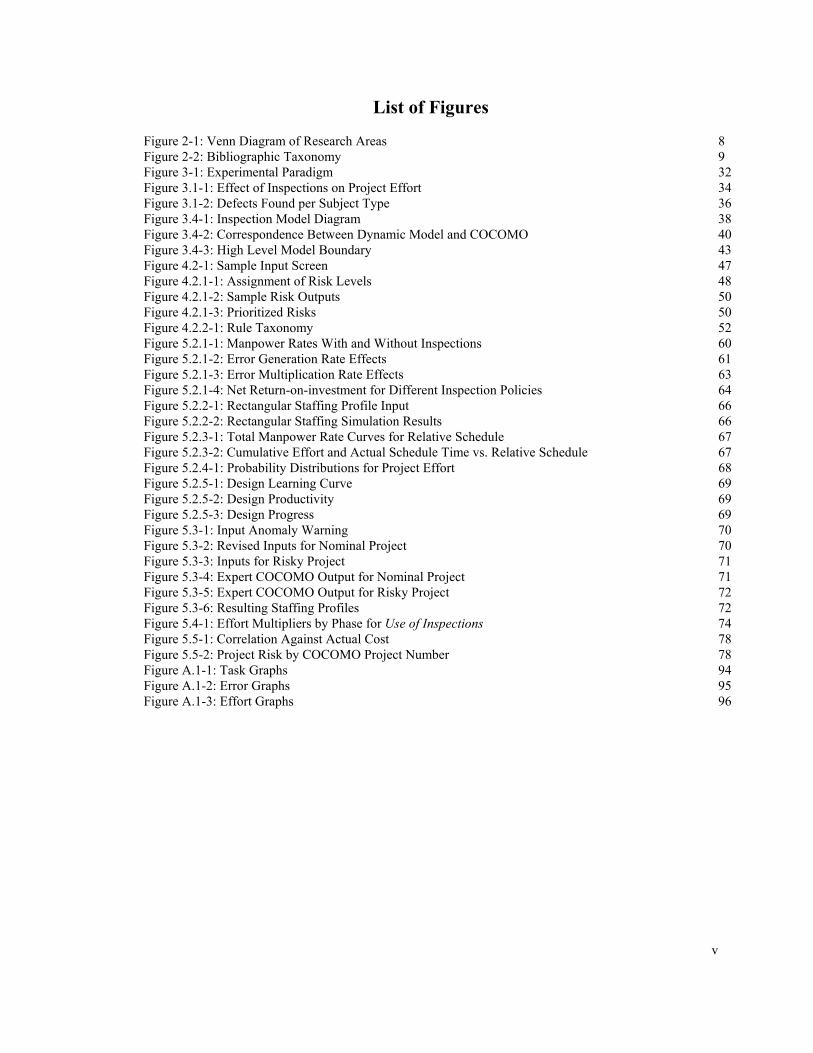
List of Figures Figure 2-1: Venn Diagram of Research Areas 8 Figure 2-2: Bibliographic Taxonomy 9 Figure 3-1: Experimental Paradigm 32 Figure 3.1-1: Effect of Inspections on Project Effort 34 Figure 3.1-2: Defects Found per Subject Type 36 Figure 3.4-1: Inspection Model Diagram 38 Figure 3.4-2: Correspondence Between Dynamic Model and COCOMO 40 Figure 3.4-3: High Level Model Boundary 43 Figure 4.2-1: Sample Input Screen 47 Figure 4.2.1-1: Assignment of Risk Levels 48 Figure 4.2.1-2: Sample Risk Outputs 50 Figure 4.2.1-3: Prioritized Risks 50 Figure 4.2.2-1: Rule Taxonomy 52 Figure 5.2.1-1: Manpower Rates With and Without Inspections 60 Figure 5.2.1-2: Error Generation Rate Effects 61 Figure 5.2.1-3: Error Multiplication Rate Effects 63 Figure 5.2.1-4: Net Return-on-investment for Different Inspection Policies 64 Figure 5.2.2-1: Rectangular Staffing Profile Input 66 Figure 5.2.2-2: Rectangular Staffing Simulation Results 66 Figure 5.2.3-1: Total Manpower Rate Curves for Relative Schedule 67 Figure 5.2.3-2: Cumulative Effort and Actual Schedule Time vs. Relative Schedule 67 Figure 5.2.4-1: Probability Distributions for Project Effort 68 Figure 5.2.5-1: Design Learning Curve 69 Figure 5.2.5-2: Design Productivity 69 Figure 5.2.5-3: Design Progress 69 Figure 5.3-1: Input Anomaly Warning 70 Figure 5.3-2: Revised Inputs for Nominal Project 70 Figure 5.3-3: Inputs for Risky Project 71 Figure 5.3-4: Expert COCOMO Output for Nominal Project 71 Figure 5.3-5: Expert COCOMO Output for Risky Project 72 Figure 5.3-6: Resulting Staffing Profiles 72 Figure 5.4-1: Effort Multipliers by Phase for Use of Inspections 74 Figure 5.5-1: Correlation Against Actual Cost 78 Figure 5.5-2: Project Risk by COCOMO Project Number 78 Figure A.1-1: Task Graphs 94 Figure A.1-2: Error Graphs 95 Figure A.1-3: Effort Graphs 96

v

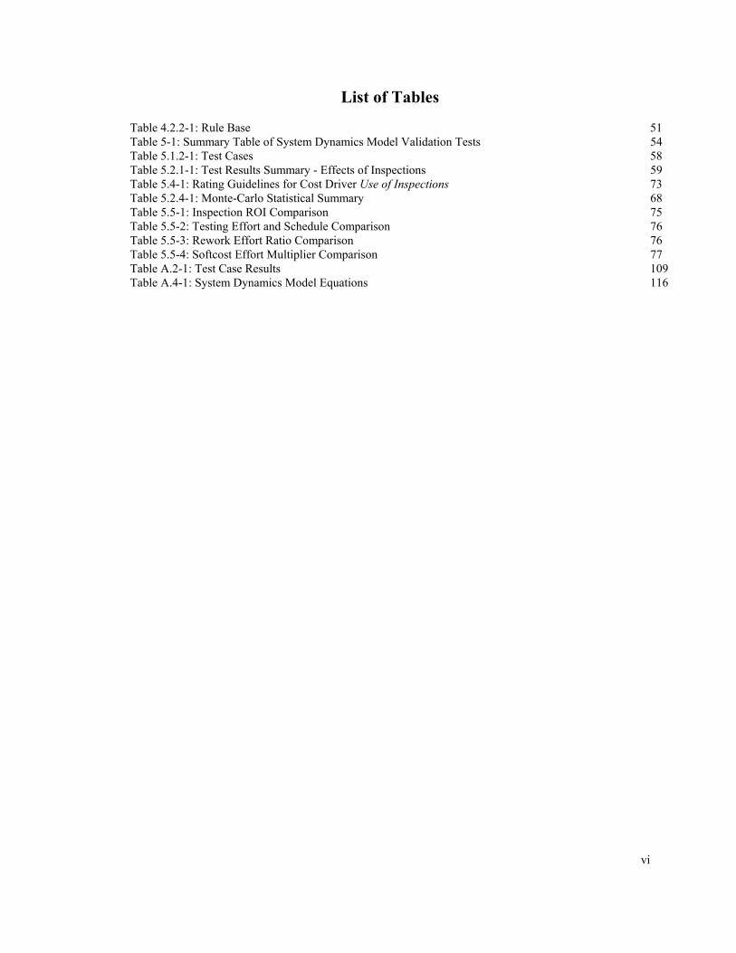
List of Tables

Table 4.2.2-1: Rule Base 51 Table 5-1: Summary Table of System Dynamics Model Validation Tests 54 Table 5.1.2-1: Test Cases 58 Table 5.2.1-1: Test Results Summary - Effects of Inspections 59 Table 5.4-1: Rating Guidelines for Cost Driver Use of Inspections 73 Table 5.2.4-1: Monte-Carlo Statistical Summary 68 Table 5.5-1: Inspection ROI Comparison 75 Table 5.5-2: Testing Effort and Schedule Comparison 76 Table 5.5-3: Rework Effort Ratio Comparison 76 Table 5.5-4: Softcost Effort Multiplier Comparison 77 Table A.2-1: Test Case Results 109 Table A.4-1: System Dynamics Model Equations 116

vi

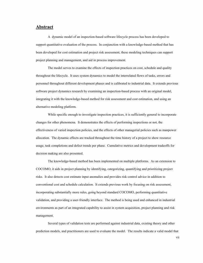
Abstract

A dynamic model of an inspection-based software lifecycle process has been developed to

support quantitative evaluation of the process. In conjunction with a knowledge-based method that has

been developed for cost estimation and project risk assessment, these modeling techniques can support

project planning and management, and aid in process improvement.

The model serves to examine the effects of inspection practices on cost, schedule and quality

throughout the lifecycle. It uses system dynamics to model the interrelated flows of tasks, errors and

personnel throughout different development phases and is calibrated to industrial data. It extends previous

software project dynamics research by examining an inspection-based process with an original model,

integrating it with the knowledge-based method for risk assessment and cost estimation, and using an

alternative modeling platform.

While specific enough to investigate inspection practices, it is sufficiently general to incorporate

changes for other phenomena. It demonstrates the effects of performing inspections or not, the

effectiveness of varied inspection policies, and the effects of other managerial policies such as manpower

allocation. The dynamic effects are tracked throughout the time history of a project to show resource

usage, task completions and defect trends per phase. Cumulative metrics and development tradeoffs for

decision making are also presented.

The knowledge-based method has been implemented on multiple platforms. As an extension to

COCOMO, it aids in project planning by identifying, categorizing, quantifying and prioritizing project

risks. It also detects cost estimate input anomalies and provides risk control advice in addition to

conventional cost and schedule calculation. It extends previous work by focusing on risk assessment,

incorporating substantially more rules, going beyond standard COCOMO, performing quantitative

validation, and providing a user-friendly interface. The method is being used and enhanced in industrial

environments as part of an integrated capability to assist in system acquisition, project planning and risk

management.

Several types of validation tests are performed against industrial data, existing theory and other

prediction models, and practitioners are used to evaluate the model. The results indicate a valid model that

vii

can be used for process evaluation and project planning, and serve as a framework for incorporating other

dynamic process factors.

viii

Chapter 1 Introduction

This study extends knowledge in the fields of software project dynamics modeling, process

technology, cost estimation and risk management. It is a significant contribution because explication of the

dynamic interdependencies of software project variables fills in knowledge gaps in these fields to produce

an integrated model of their relationships.

A large knowledge gap exists for measuring different software development practices and

planning large software projects. There are virtually no methods of quantitatively comparing dynamic

characteristics of software development processes and few for assessing project risk. Very little data exists

on the tradeoffs of alternative software development process models, and expert knowledge is not utilized

in tool assistants for cost and schedule estimation or project risk assessment.

This research investigates system dynamics modeling of alternative software development

processes and knowledge-based techniques for cost, schedule and risk assessment of large software

projects with a primary focus on cost. In particular, an inspection-based development process is modeled.

By combining quantitative techniques with expert judgement in a common model, an intelligent simulation

capability results to support planning and management functions for software development projects. This

provides greater insight into the software development process, increased estimation and risk management

capabilities to reduce project cost and schedule variances, and the capability to evaluate process

improvement via process definition and analysis. The overall project assessment toolset provides a

framework for software cost/schedule/risk management and process maturity improvement across software

development organizations.

The system dynamics model employs feedback principles to simulate dynamic interactions of

management decision-making processes and technical development activities. Dynamic modeling of the

software development process has provided a number of useful insights, and can be used to predict the

consequences of various management actions or test the impact of internal or external environmental

factors. By having an executable simulation model, managers can assess the effects of changed processes

and management policies before they commit to development plans.

1

A calibrated dynamic model enables a metrics-based continuous process improvement capability,

and a basis for prioritizing organizational process improvement investments by providing a measure of

software development processes. The process model can be used as a baseline for benchmarking process

improvement metrics.

The knowledge-based component of this study incorporates expert heuristics to assess various

facets of cost and schedule estimation and project risk assessment based on cost factors. Incorporation of

expert system rules can place considerable added knowledge at the disposal of the software project planner

or manager to help avoid high-risk development situations and cost overruns.

1.1 Statement of the Problem

The main problem investigated in this research is what are the effects of changes to the software

development process on cost, schedule and risk? In particular, the effects of performing inspections during

the process are investigated. The rationale for this study is to improve software engineering practice.

Some general definitions are provided below before expanding on the problem and purpose:

software engineering: the discipline in which science and mathematics are applied in developing software

process: a set of activities, methods, practices, and transformations that people use to develop and maintain

software and the associated products [Paulk et al. 91]

inspection: a formal review of a software artifact such as design or code to efficiently find errors. An

inspection requires training of participants, sufficient preparation time before an inspection meeting, a

structured meeting with timing and defect recording protocols, specific roles executed during the meeting,

and followup of fixing defects found during the inspection. See Chapter 3 for more details of inspections

including the effort required to perform them.

cost estimation: prediction of both the person effort and elapsed time of a project

risk: the possibility of an unsatisfactory outcome on a project

knowledge-based system: a program that operates on captured knowledge and expertise using inference to

emulate human reasoning.

2

The term "process model" has two distinct interpretations in this research. A process model refers to 1) a

method of software development, i.e. a lifecycle process model that determines the order of the stages

involved in software development and evolution, and establishes the transition criteria for progressing

between stages and 2) an executable simulation model of the software development process. This research

develops a simulation model of a software development method. Proper interpretation of the term will be

made clear in context.

Some specific sets of questions addressed by this research include the following:

1) What are the dynamic effects of process changes on cost, schedule, risk and related factors? What are

the quantitative and qualitative (heuristic) features of an inspection-based process from a cost/schedule/risk

perspective?

2) Which expert heuristics using cost factors are useful for risk assessment? To what extent can they be

quantified? Can knowledge-based project risk assessment in the form of heuristic rules be combined with

a dynamic model? What are some common factors that can be used to link the risk assessment and

dynamic modeling?

3) What are the relationships between dynamic and static models and how are they complementary? How

can the results of static models contribute to dynamic models? Can a dynamic model be calibrated such

that a point prediction will always match that of a static model?

To delimit the scope of this research, only medium to large size software projects are considered.

These typically fall in the range of 50,000 to 1,000,000 delivered lines of code [Charette 89]. Only an

inspection-based development processes will be modeled, as identified in subsequent sections.

The practice of software engineering is multi-faceted with a host of interrelated problems, and this

research explores methods to help alleviate some of these problems. The remainder of this section

describes these problems and the relevance of this study for helping to solve them.

1.2 Purpose of the Research

3

The role of software in complex systems has increased dramatically over the last couple of

decades. Software is often the critical factor in project success, and companies are recognizing software as

the key to competitiveness. Software is normally the control center of complex architectures, provides

system flexibility and increasingly drives hardware design. Though there have been substantial

advancements in software practices, there are difficult development problems that will pose increasing

challenges for a long time.

The magnitude of software development has increased tremendously; the annual cost is now

estimated at $200B in the United States alone. As the problems to be solved increase in complexity,

systems grow in size and hardware performance increases, the task of software development for large and

innovative systems becomes more difficult to manage. Despite these obstacles, the software demand

continues to increase at a substantial rate.

The term software crisis refers to a set of various problems associated with the software

development of large systems that meet their requirements and are cost effective, timely, efficient, reliable

and modifiable. Escaping from a software crisis can be accomplished by improving the organizational

process by which software is created, maintained and managed [Humphrey 89].

One of the first books to highlight the process problem was The Mythical Man-Month [Brooks 75]

where the problems were identified as not just product failures but failures in the development process

itself. In the ensuing years, software has become the medium of new systems in a much larger way.

Development of complex systems is increasingly reliant on software development practices as the

proportion of software to hardware development effort has transitioned from a small part to the sizable

majority [Charette 89, Boehm 89].

Tools are needed to assist in alleviating the problems associated with the development of large,

complex software systems. Planning and management are at the core of the problems due to a lack of

understanding of the development process coupled with the increasing size and complexity demanded of

systems. Much of the difficulty of development can be mitigated by effectively applying appropriate

engineering methods and tools to management practices. Much focus is on improving technical

4

development activities, but without corresponding advances in software management tools and practices,

software projects will continue to produce cost overruns, late deliveries and dissatisfied customers.

Many techniques have been developed and used in software development planning. Besides cost

models, other well-known methods include Critical Path Method/Program Evaluation and Review

Techniques (CPM/PERT), decision analysis and others [Boehm 89, Pressman 87]. These methods all have

limitations. CPM/PERT methods can model the detailed development activities and cost estimation models

produce estimates used for initial planning, but none of these techniques model the dynamic aspects of a

project such as managerial decision making and software development activities in a micro-oriented

integrative fashion.

Typical problems in software development include poor cost and schedule estimation,

unreasonable planning, lack of risk identification and mitigation, constantly shifting requirements

baselines, poor hiring practices, and various difficulties faced by developers prolonged by a lack of

managerial insight. These problems are related in important ways, and explication of the

interdependencies can provide knowledge and techniques for assistance.

A major research problem is how to identify and assess risk items. Risks on software projects can

lead to cost overruns, schedule slip, or poorly performing software. Risk factors are frequently built into

problem-ridden software projects via oversimplified assumptions about software development, such as

assuming the independence of individual project decisions and independence of past and future project

experience.

Project planners often overlook risk situations when developing cost and schedule estimates.

After the proposal or project plan is approved, the software development team must live with the built-in

risk. These initial project plans are usually not revised until it's too late to influence a more favorable

outcome. By incorporating expert knowledge, these risks can be identified during planning and mitigated

before the project begins.

Many of the aforementioned problems can be traced to the development process. The traditional

waterfall process has been blamed for many of the downfalls. It prescribes a sequential development cycle

of activities whereby requirements are supposed to be fixed at the beginning. Yet requirements are

5

virtually never complete at project inception. The problems are exacerbated when this occurs on a large,

complex project. Changes to requirements are certain as development progresses, thereby leading to

substantial cost and schedule inefficiencies in the process. Other problems with the traditional waterfall

include disincentives for reuse, lack of user involvement, inability to accommodate prototypes, and more

[Agresti 86, Boehm 88].

In recent years, a variety of alternative process models have been developed to mitigate such

problems. However, project planners and managers have few if any resources to evaluate alternative

processes for a proposed or new project. Very few software professionals have worked within more than

one or two types of development processes, so there is scant industrial experience to draw on in

organizations at this time. Different process models, particularly the newer ones of interest, are described

in section 2.1.1.1 Process Lifecycle Models.

When considering potential process changes within the decision space of managers, it would be

desirable to predict the impact via simulation studies before choosing a course of action. The use of a

simulation model to investigate these different software development practices and managerial decision

making policies will furnish managers with added knowledge for evaluating process options, provide a

baseline for benchmarking process improvement activities, and more accurate prediction capability.

As described, methods are needed to provide automated assistance in the areas of process

evaluation and risk assessment to support planning and management of large projects. Given the

magnitude of software development, even incremental and partial solutions can provide significant returns.

6

Chapter 2 Background

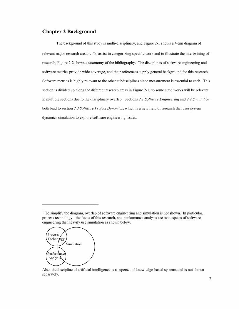
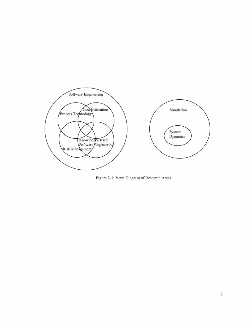
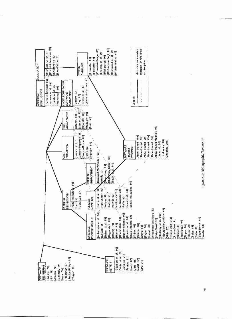
The background of this study is multi-disciplinary, and Figure 2-1 shows a Venn diagram of

relevant major research areas1. To assist in categorizing specific work and to illustrate the intertwining of

research, Figure 2-2 shows a taxonomy of the bibliography. The disciplines of software engineering and

software metrics provide wide coverage, and their references supply general background for this research.

Software metrics is highly relevant to the other subdisciplines since measurement is essential to each. This

section is divided up along the different research areas in Figure 2-1, so some cited works will be relevant

in multiple sections due to the disciplinary overlap. Sections 2.1 Software Engineering and 2.2 Simulation

both lead to section 2.3 Software Project Dynamics, which is a new field of research that uses system

dynamics simulation to explore software engineering issues.

________________________ 1 To simplify the diagram, overlap of software engineering and simulation is not shown. In particular, process technology - the focus of this research, and performance analysis are two aspects of software engineering that heavily use simulation as shown below.

Simulation

Performance Analysis

ProcessTechnology

Also, the discipline of artificial intelligence is a superset of knowledge-based systems and is not shown separately.

7

SystemDynamics

Simulation

Knowledge-BasedSoftware Engineering

Risk Management

Cost EstimationProcess Technology

Software Engineering

Figure 2-1: Venn Diagram of Research Areas

8

2.1 Software Engineering

An early definition of software engineering was "the establishment and use of sound engineering

principles in order to obtain economically software that is reliable and works efficiently on real machines"

[Naur 69]. Boehm adds the provision of human utility in the definition "software engineering is the

application of science and mathematics by which the capabilities of computer equipment are made useful to

man via computer programs, procedures and associated documentation" [Boehm 81]. In practice, the

engineering principles are applied as a combination of different methods. This research investigates new

methods to assist in software engineering, and the following subsections provide background on relevant

subdisciplines.

2.1.1 Process Technology

Software process technology is a new field being used to address several critical issues in software

engineering, where a process is a sequence of software development activities using associated tools and

methods. Process technology encompasses three general classes of research: new process lifecycle models,

process modeling and process improvement. This research involves all of these, since modeling of

lifecycle processes is used to achieve process improvement. Background for each of these areas is

described in separate sections.

2.1.1.1 Process Lifecycle Models

A process lifecycle model determines the order of the stages involved in software development,

and establishes the transition criteria between stages. The process used in the initial days of software

development is now called the "code-and-fix" model [Boehm 88]. It essentially contained two steps: 1)

write code and 2) fix the problems in the code. Requirements, design, test and maintenance were not

considered before coding began. This type of development led to poorly structured code that was

expensive to fix and did not match users' requirements. These problems led to the recognition of the

testing and maintenance phases, and early planning. The stagewise model, where software was to be

developed in successive stages, came about to address the deficiencies of the code-and-fix model [Boehm

88].

10

The waterfall model was first documented by Royce [Royce 70]. It offered two primary

enhancements to the stagewise model: 1) feedback loops between stages and 2) a "build it twice" step

parallel with requirements analysis [Boehm 88]. Variations of the waterfall model all contain the essential

activities of specification, design, code, test and operations/maintenance. The lifecycle model was further

popularized by Boehm in a version that contained verification, validation or test activity at the end of each

phase to ensure that the objectives of the phase were satisfied [Boehm 76]. In this model, the phases are

sequential, none can be skipped and baselines are produced throughout the phases. No changes to

baselines are made unless all interested parties agree. The economic rationale for the model is that to

achieve a successful product, all of the subgoals within each phase must be met and that a different

ordering of the phases will produce a less successful product [Boehm 81]. Another primary virtue of the

waterfall model is its recognition of design as a critical activity [Agresti 86].

However, the waterfall model implies a sequential approach to product development, which is

often impractical for large projects due to shifting requirements. Some other critiques of the waterfall

model include: a lack of user involvement, ineffectiveness in the requirements phase, inflexibility to

accommodate prototypes, unrealistic separation of specification from design, inability to accommodate

reuse, and various maintenance related problems [Agresti 86], [Boehm 88]. In [Swartout-Balzer 82], it is

argued that specification and design are inevitably intertwined, which implies that process models should

reflect this reality. Agresti claims that the fundamental weakness of the waterfall model is the imbalance of

analysis versus synthesis due to the influence of the systems approach and the reality of software practices

when the model was formulated [Agresti 86]. An annotated bibliography of critiques of the conventional

lifecycle is provided in [Agresti 86].

Some of the difficulties of the conventional (waterfall) lifecycle have been addressed by extending

it for incremental development, parallel developments, evolutionary change and other revisions and

refinements [Boehm 88, Agresti 86]. Agresti describes the prototyping, operational specification and

transformational paradigms as alternatives to the waterfall [Agresti 86]. These are shown to respond to the

inadequacies of the waterfall by delivering executable objects early to the user and increasing the role of

automation. The following sections describe selected enhancements and alternatives to the waterfall model.

11

Note that process models can be synthesized into hybrid approaches depending on the development

situation.

Prototyping is a process that enables the developer to create a quick initial working model of the

software to be built, and is similar to the "build it twice" step in Royce's 1970 waterfall model. A formal

definition of prototyping is "a full-scale model and functional form of a new system or subsystem. (A

prototype does not have to be the complete system - only the part of interest)" [Thayer-Dorfman 1990].

The objective of prototyping is to clarify the characteristics and operation of a system [Agresti 86]. This

approach may be used when there is only a general set of objectives, or other uncertainties exist about

algorithmic efficiencies or the desired form of an interface. A quick design occurs focusing on software

aspects visible to the user, and the resulting prototype is evaluated to refine the requirements [Boehm 89,

Pressman 87].

The incremental process approach develops a system in increments, whereby all requirements are

determined up front and subsets of requirements are allocated to separate increments. The increments are

developed in sequential cycles, with each incremental release adding functionality. One example is as the

Ada process model [Boehm 89a, Royce 90] which uses salient features of Ada to mitigate risks, such as the

ability to compile specifications of design early on. The incremental approach reduces overall effort and

provides an initial system earlier to the customer. The effort phase distributions are different and the

overall schedule may lengthen somewhat [Boehm 81]. The Ada process model prescribes more effort in

requirements analysis and design, and less for coding and integration.

Inspections are a formal, efficient and economical method of finding errors in design and code

[Fagan 76]. They are a form of peer review, as are structured walkthroughs. An inspection-based process

uses inspections at a number of points in the process of project planning and system development, and thus

can be used for requirements descriptions, design, code, test plans, or virtually any engineering document.

Inspections are carried out in a prescribed series of steps including preparation, having an

inspection meeting where specific roles are executed, and rework of errors discovered by the inspection.

By detecting and correcting errors in earlier stages of the process such as design, significant cost reductions

can be made since the rework is much less costly compared to later in the testing and integration phases

12

[Radice-Phillips 88, Grady 92, Madachy et al. 93a]. Further background and a model of the inspection-

based process is discussed in Chapter 3 Modeling of an Inspection-Based Process.

The transform model automatically converts a formal software specification into a program

[Balzer et al. 83]. Such a model minimizes the problems of code that has been modified many times and is

difficult to maintain. The steps involved in the transform process model identified in [Boehm 88] are: 1)

formally specify the product, 2) automatically transform the specification into code (this assumes the

capability to do so), 3) iterate if necessary to improve the performance, 3) exercise the product and 4)

iterate again by adjusting the specification based on the operational experience. This model and its variants

are often called operational specification or fourth-generation language (4GL) techniques.

The evolutionary model was developed to address deficiencies in the waterfall model related to

having fully elaborated specifications [McCracken-Jackson 83]. The stages in the evolutionary model are

expanding increments of an operational product, with evolution being determined by operational

experience. Such a model helps deliver an initial operational capability and provides a real world

operational basis for evolution; however, the lack of long-range planning often leads to trouble with the

operational system not being flexible enough to handle unplanned paths of evolution [Boehm 88].

The spiral model can accommodate previous models as special cases and provides guidance to

determine which combination of models best fits a given situation [Boehm 88]. It is a risk-driven method

of development that identifies areas of uncertainties that are sources of project risk. The development

proceeds in repeating cycles of determining objectives, evaluating alternatives, prototyping and

developing, and then planning the next cycle. Each cycle involves a progression that addresses the same

sequence of steps for each portion of the product and for each level of elaboration. Development builds on

top of the results of previous spirals. This is in contrast to the waterfall model which prescribes a single

shot development where documents are the criteria for advancing to subsequent development stages. The

spiral model prescribes an evolutionary process, but explicitly incorporates long-range architectural and

usage considerations in contrast to the basic evolutionary model [Boehm 88].

A number of proposed reuse process models have been published. Some are risk-driven and

based on the spiral model, while others are enhanced waterfall process models. Those based on the spiral

13

model have only mapped partial activities onto the spiral [Prieto-Diaz 91a], or adapted the model to a

specific application domain [Danner 91]. A set of process models has been proposed by Cohen at the

Software Engineering Institute for different levels of reuse: adaptive, parameterized and engineered [Cohen

91].

A process for reusing software assets provides reduced development time, improved reliability,

improved quality and user programmability [Boehm-Scherlis 92]. A software process model for reuse and

re-engineering must provide for a variety of activities and support the reuse of assets across the entire

lifecycle. Such assets may include requirements, architectures, code, test plans, QA reviews, documents,

etc. It must support tasks specific to reuse and re-engineering, such as domain analysis and domain

engineering [Prieto-Diaz 91]. Re-engineering differs from reuse in that entire product architectures are

used as starting points for new systems, as opposed to bottom-up reuse of individual components. In

[Boehm-Scherlis 92], the term megaprogramming is given to the practice of building and evolving

software component by component. It incorporates reuse, software engineering environments, architecture

engineering and application generation to provide a product-line approach to development [Boehm-

Scherlis 92].

The cleanroom process approach [Mills 87] certifies the reliability of a software system based on

a certification model, and is being used in several companies and government agencies. In this process,

programmers can't even compile their own code as it's done by independent workers. Much of the

traditional programming task work shifts to certification activities in this process model.

In summary, primary differences between some major models are: prototyping develops small

working models to support requirements definition, transformational approaches specify the software and

employ automatic code generation, incremental development defines all requirements up front and then

allocates requirement subsets to individual releases, evolutionary approaches also develop software in

increments except that requirements are only defined for the next release, reuse-based development uses

previously developed software assets and the spiral model is a risk-driven variation of evolutionary

development that can function as a superset process model. Some of the other identified process changes

provide alternative methods for implementing subprocesses of the more encompassing lifecycle models.

14

Few guidelines have been published to aid in selecting an appropriate process model for a given

project, though Boehm has developed a process structuring table [Boehm 89] and Sabo has developed a

knowledge-based assistant for choosing a process [Sabo 93]. One application of the spiral model was for

process generation itself [Boehm-Belz 88]. The spiral model provided an approach for determining the

requirements, architecture and design of a software development process. This research develops methods

for evaluating alternative processes including risk analysis, which are critical activities called for by the

risk-driven spiral approach to process development.

There have been a couple small experiments comparing different programming processes in terms

of productivity, resulting product size and quality. In [Boehm 88a], an experiment was performed

comparing development teams that used prototyping versus writing requirements specifications. In [Davis

88], an initial framework was developed for comparing lifecycle models. The comparison framework was

a non-quantitative approach for visualizing differences between models in terms of the ability to meet

user's functional needs. These studies were both preliminary, did not consider dynamic project

interactions, provided little data and no tool support that project planners can utilize, and stressed the need

for further research to quantify the tradeoffs.

2.1.1.2 Process Modeling

Osterweil has argued that we should be as good at modeling the software process as modeling

applications [Osterweil 87]. Process modeling is representing a process architecture, design or definition

in the abstract [Feiler-Humphrey 93]. Software process modeling supports process-driven development

and related efforts such as process definition, process improvement, process management and automated

process-driven environments [Curtis et al. 92, Kellner 92]. As a means of reasoning about software

processes, process models provide a mechanism for recording and understanding processes, evaluating,

communicating and promoting process improvements. Thus, process models are a vehicle for improving

software engineering practice.

To support the above objectives, process models must go beyond representation to support

analysis of a process including the prediction of potential process changes and improvements [Kellner 91,

15

Feiler-Humphrey 93]. Unfortunately, there is no standard approach for process modeling. A variety of

process definition and simulation methods exist that answer unique subsets of process questions.

Software process modeling is distinguished from other types of modeling in computer science

because many of the phenomena are enacted by humans [Curtis et al. 92]. Research on software process

modeling supports a wide range of objectives including facilitating human understanding and

communication, supporting process improvement, supporting process management, automating process

guidance and automating execution support [Curtis et al. 92]. A background of process improvement is

provided in the next section, 2.1.1.3 Process Improvement.

This research uses process modeling to support several of the aforementioned objectives,

particularly process improvement and process management. It will also help facilitate human

understanding and communication of the process, but does not explicitly consider automated process

guidance or automated execution support.

Process modeling languages and representations usually present one or more perspectives related

to the process. Some of the most commonly represented perspectives are functional, behavioral,

organizational and informational. They are analogous to different viewpoints on an observable process.

Although separate, these representations are interrelated and a major difficulty is tying them together

[Curtis et al. 92, Kellner 91, Kellner 92].

There have been a host of language types and constructs used in software process modeling to

support the different objectives and perspectives. Five approaches to representing process information, as

described and reviewed in [Curtis et al. 92] are programming models (process programming), functional

models, plan-based models, Petri-net models (role interaction nets) and quantitative modeling (system

dynamics). The suitability of a modeling approach depends on the goals and objectives for the resulting

model. No current software process modeling approach fully satisfies the diverse goals and objectives

previously mentioned [Kellner 91].

Functional models have been developed with the Hierarchical and Functional Software Process

(HFSP) description and enaction language [Suzuki-Katayama 91]. HFSP is primarily a declarative and

textual language. A process is defined as a set of mathematical relationships among inputs (such as

16

specifications) and outputs (such as source code). HFSP is primarily oriented towards the functional and

behavioral perspectives.

Plan-based models have been implemented in a constraint-based language called GRAPPLE

[Huff-Lessor 89]. It models software development as a set of goals, subgoals, preconditions, constraints

and effects. An effective plan-based process model requires coding information of the environment and

the goal hierarchies of the process.

The role interaction structure of a project can be represented by a Petri-net based representation.

Interaction nets can be used to coordinate the routing of artifacts among interacting roles and can be used

to track progress as the completions of role interactions. There have been problems with scalability and

using the technique if a basic description of the organization process does not already exist [Curtis et al.

92].

System dynamics is one of the few modeling techniques that involves quantitative representation.

Feedback and control system techniques are used to model social and industrial phenomena. See section

2.2.1 System Dynamics for more background on system dynamics and section 2.3 Software Project

Dynamics for research that uses system dynamics to model behavioral aspects of software projects.

Dynamic behavior, as modeled through a set of interacting equations, is difficult to reproduce

through modeling techniques that do not provide dynamic feedback loops. The value of system dynamics

models are tied to the extent that constructs and parameters represent actual observed project states [Curtis

et al. 92].

A process modeling approach that combines several language paradigms has been developed by

Kellner and colleagues at the Software Engineering Institute (SEI) [Kellner 90, Kellner 91, Kellner 92]. It

utilizes the STATEMATE tool that includes state transitions with events and triggers, systems analysis and

design diagrams and data modeling to support representation, analysis and simulation of processes. This

approach enables a quantitative simulation that combines the functional, behavioral and organizational

perspectives.

17

The modeling approach was used for an example process, investigating quantitative aspects of

managerial planning [Kellner 91]. In the micro-level study, specific coding and testing tasks with assumed

task durations and outcomes were used to derive schedules, work effort and staffing profiles.

Another technique for process modeling is the Articulator approach developed by Mi and Scacchi

[Mi-Scacchi 91, Mi-Scacchi 92, Scacchi-Mi 93]. They have developed a knowledge-based computing

environment that uses artificial intelligence scheduling techniques from production systems for modeling,

analyzing and simulating organizational processes. Classes of organizational resources are modeled using

an object-oriented knowledge representation scheme. The resource classes characterize the attributes,

relations, rules and computational methods used. The resource taxonomy serves as a meta-model for

constructing process models consisting of agents, tools and tasks. Consistency, completeness and

traceability of the process can be analyzed with the Articulator approach, and simulation takes place

through the symbolic performance of process tasks by assigned agents using tools and other resources.

2.1.1.3 Process Improvement

In order to address software development problems, the development task must be treated as a

process that can be controlled, measured and improved [Humphrey 89]. This requires an organization to

understand the current status of their processes, identify desired process change, make a process

improvement plan and execute the plan.

Humphrey has developed a model of how software organizations can mature their processes and

continually improve to better meet their cost and schedule goals called the Capability Maturity Model

(CMM) [Humphrey 89]. The CMM framework identifies five levels of organizational maturity, where

each level lays a foundation for making process improvements at the next level. The framework utilizes a

set of key practices including requirements management, project planning and control, quality assurance,

configuration management, process focus and definition, process measurement and analysis, quality

management and others. The SEI, tasked by the government to improve software engineering practices, is

using the CMM as a basis for improving the software processes of organizations [Paulk et al. 91].

At level one in the CMM, an organization is described as ad-hoc, whereby processes are not in

place and a chaotic development environment exists. The second level is called the repeatable level. At

18

this level, project planning and tracking is established and processes are repeatable. The third level is

termed the defined level, whereby processes are formally defined. Level 4 is called the managed level,

whereby the defined process is instrumented and metrics are used to set targets. Statistical quality control

can then be applied to process elements. At level 5, the optimized level, detailed measurements are used to

guide programs of continuous process improvement, technology innovation and defect prevention.

To make the process predictable, repeatable and manageable, an organization must first assess the

maturity of the processes in place [Paulk et al. 91]. By knowing the maturity level, organizations can

identify problem areas to concentrate on and effect process improvement in key practice areas. The SEI

has developed assessment procedures based on the CMM [Humphrey-Sweet 87].

Software process modeling is essential to support process improvements at levels 4 and 5 through

process definition and analysis. Process models can represent the variation among processes, encapsulate

potential solutions and can be used as a baseline for benchmarking process improvement metrics [Lai 93].

In [Grady 92], guidelines for collecting and analyzing metrics to support process improvement are

provided.

2.1.2 Cost Estimation

Cost models are commonly used for project planning and estimation. The most widely accepted

and thoroughly documented software cost model is Boehm's COnstructive COst MOdel (COCOMO)

presented in his landmark book on software engineering economics [Boehm 81]. The model is

incorporated in many of the estimation tools used in industry and research. The multi-level model provides

formulas for estimating effort and schedule using cost driver ratings to adjust the estimated effort. It is

also used to compute the initial project plan for Abdel-Hamid's dynamic project simulation [Abdel-Hamid-

Madnick 91].

The COCOMO model estimates software effort as a nonlinear function of the product size and

modifies it by a geometric product of effort multipliers associated with cost driver ratings. The cost driver

variables include product attributes, computer attributes, personnel attributes and project attributes. In the

most detailed version of COCOMO, the effort multipliers are phase-sensitive, thus taking on different

19

values throughout the various phases of the project. The revised Ada COCOMO model adds some more

cost drivers, including process attributes [Boehm-Royce 89].

In terms of prediction capability against the COCOMO database, the Basic version of COCOMO

which does not incorporate cost drivers estimates within 20% of project actuals only 25% of the time. The

Intermediate version incorporating cost drivers predicts within 20% of actuals 68% of the time. The

prediction increases to 70% of the time for the Detailed version. This prediction performance represents

the approximate upper range of current cost models [Boehm 81, Conte et al. 86, Charette 89].

While COCOMO is an empirical model incorporating analytic equations, statistical data fitting

and expert judgement, other cost models are more theoretically based [Conte et al. 86]. Putnam's resource

allocation model called SLIM assumes that manpower utilization follows a Rayleigh-type curve [Putnam

80]. Jensen's model is similar to Putnam's model, but it attempts to soften the effect of schedule

compression on effort. The RCA PRICE S is another composite model like COCOMO geared towards

embedded system applications. Several other models have been proposed throughout the years that are

algorithmic, top-down, bottom-up, Parkinsonian and other types.

2.1.3 Risk Management

Risk is the possibility of undesirable outcome, or a loss. Risk impact, or risk exposure is defined

as the probability of loss multiplied by the cost of the loss. Risk management is a new discipline whose

objectives are to identify, address and eliminate software risk items before they become either threats to

successful software operation or major sources of software rework [Boehm 89].

Examples of risk in software development include exceeding budget, schedule overrun, or

delivering an unsuitable product. Boehm identifies the top 10 generic software risk items in [Boehm 89],

and Charette provides documented evidence of many software development failures to highlight the need

for risk management practice [Charette 89].

Software risk management involves a combination of methods used to assess and control risk, and

is on ongoing activity throughout a development project. Some common techniques used include

performance models, cost models, network analysis, decision analysis, quality factor analysis and others

[Boehm 89, Rook 93]. Risk management involves both risk assessment and risk control [Boehm 89,

20

Charette 89]. The substeps in risk assessment are risk identification, risk analysis and risk prioritization,

whereas risk control entails risk management planning, risk resolution and risk monitoring.

Risk identification produces a list of risk items, risk analysis evaluates the magnitudes of loss

probability and consequence, and risk prioritization produces an ordered list of the risk items by severity.

Risk management planning is the creation of plans to address specific risk items, risk resolution is creating

a situation that eliminates or lessens a given risk, and risk monitoring is tracking of the risk resolution

activities [Boehm 89].

Risk management attempts to balance the triad of cost-schedule-functionality [Charette 89,

Boehm 89]. Though cost, schedule and product risks are interrelated, they can also be analyzed

independently. Some methods used to quantify cost, schedule and performance risk include table methods,

analytical methods, knowledge based techniques, questionnaire-based methods and others.

A risk identification scheme has been developed by the SEI that is based on a risk taxonomy [Carr

et al. 93]. A hierarchical questionnaire is used by trained assessors to interview project personnel.

Different risk classes are product engineering, development environment and program constraints [Carr et

al. 93].

Knowledge-based methods can be used to assess risk and provide advice for risk mitigation. In

Chapter 4, a risk assessment scheme is described that uses cost factors from COCOMO to identify risk

items from [Madachy 94]. Toth has developed a method for assessing technical risk based on a knowledge

base of product and process needs, satisfying capabilities and capability maturity factors [Toth 94]. Risk

areas are inferred by evaluating disparities between needs and capabilities.

Risk management is heavily allied with cost estimation [Boehm 89, Charette 89, Rook 93]. Cost

estimates are used to evaluate risk and perform risk tradeoffs, risk methods such as Monte Carlo simulation

can be applied to cost models, and the likelihood of meeting cost estimates depends on risk management.

The spiral model is often called a risk-driven approach to software development [Boehm 88], as

opposed to a document-driven or code-driven process such as the waterfall. Each cycle through the spiral

entails evaluation of the risks. Thus, the spiral model explicitly includes risk management in the process.

21

Risk management bridges concepts from the spiral model with software development practices [Boehm

88].

Performing inspections is a method of reducing risk. By reviewing software artifacts before they

are used in subsequent phases, defects are found and eliminated beforehand. If practiced in a rigorous and

formal manner, inspections can be used as an integral part of risk management.

2.1.4 Knowledge-Based Software Engineering

Recent research in knowledge-based assistance for software engineering is on supporting all

lifecycle activities [Green et al. 87], though much past work has focused on automating the coding process.

Progress has been made in transformational aids to development, with much less progress towards

accumulating knowledge bases for large scale software engineering processes [Boehm 92]. Despite the

potential of capturing expertise to assist in project management of large software developments, few

applications have specifically addressed such concerns. Knowledge-based techniques have been used to

support automatic programming [Lowry-McCartney 91], risk analysis, architecture determination, and

other facets of large scale software development. Some recent work has been done on relevant

applications including risk management and process structuring.

Using a knowledge base of cost drivers for risk identification and assessment is a powerful tool.

Common patterns of cost and schedule risk can be detected this way. An expert systems cost model was

developed at Mitre [Day 87] employing about 40 rules with the COCOMO model, though it was used very

little. Expert COCOMO is a knowledge-based approach to identifying project risk items related to cost

and schedule and assisting in cost estimation [Madachy 94]. This work extends [Day 87] to incorporate

substantially more rules and to quantify, categorize and prioritize the risks. See Chapter 4 Knowledge-

Based Risk Assessment and Cost Estimation for more details on Expert COCOMO.

Toth has also developed a knowledge-based software technology risk advisor (STRA) [Toth 94],

which provides assistance in identifying and managing software technology risks. Whereas Expert

COCOMO uses knowledge of risk situations based on cost factors to identify and quantify risks, STRA

uses a knowledge base of software product and process needs, satisfying capabilities and maturity factors.

STRA focuses on technical product risk while Expert COCOMO focuses on cost and schedule risk.

22

A knowledge-based project management tool has also been developed to assist in choosing the

software development process model that best fits the needs of a given project [Sabo 93]. It also performs

remedial risk management tasks by alerting the developer to potential conflicts in the project metrics. This

work was largely based on a process structuring decision table in [Boehm 89], and operates on knowledge

of the growth envelope of the project, understanding of the requirements, robustness, available technology,

budget, schedule, haste, downstream requirements, size, nucleus type, phasing, and architecture

understanding.

2.2 Simulation

Simulation is the numerical evaluation of a model, where a model consists of mathematical

relationships describing a system of interest. Simulation can be used to explain system behavior, improve

existing systems, or to design new systems [Khoshnevis 92]. Systems are further classified as static or

dynamic, while dynamic systems can be continuous, discrete or combined depending on how the state

variables change over time. A discrete model is not always used to model a discrete system and vice-versa.

The choice of model depends on the specific objectives of a study.

23

2.2.1 System Dynamics

System dynamics refers to the simulation methodology pioneered by Forrester, which was

developed to model complex continuous systems for improving management policies and organizational

structures [Forrester 61, Forrester 68]. Models are formulated using continuous quantities interconnected

in loops of information feedback and circular causality. The quantities are expressed as levels (stocks or

accumulations), rates (flows) and information links representing the feedback loops.

The system dynamics approach involves the following concepts [Richardson 91]:

-defining problems dynamically, in terms of graphs over time

-striving for an endogenous, behavioral view of the significant dynamics of a system

-thinking of all real systems concepts as continuous quantities interconnected in information feedback

loops and circular causality

-identifying independent levels in the system and their inflow and outflow rates

-formulating a model capable of reproducing the dynamic problem of concern by itself

-deriving understandings and applicable policy insights from the resulting model

-implementing changes resulting from model-based understandings and insights.

The mathematical structure of a system dynamics simulation model is a system of coupled,

nonlinear, first-order differential equations,

x'(t) = f(x,p),

where x is a vector of levels, p a set of parameters and f is a nonlinear vector-valued function. State

variables are represented by the levels. Implementations of system dynamics include DYNAMO

[Richardson-Pugh 81], and ITHINK [Richmond et al. 90]. DYNAMO is a programming language that

requires the modeler to write difference equations. ITHINK uses visual diagramming for constructing

dynamic models, allows for graphical representation of table functions and also provides utilities for

modeling discrete components.

Although the applicability of feedback systems concepts to managerial systems has been studied

for many years, only recently has system dynamics been applied in software engineering. The following

section provides background on the use of system dynamics for modeling software development.

24

2.3 Software Project Dynamics

When used for software engineering, system dynamics provides an integrative model which

supports analysis of the interactions between related activities such as code development, project

management, testing, hiring, training, etcetera [Abdel-Hamid-Madnick 91]. System dynamics modeling of

project interactions has been shown to replicate actual project cost and schedule trends when the simulation

model is properly initialized with project parameters [Abdel-Hamid 89a, Lin et al. 92]. A dynamic model

could enable planners and managers to assess the cost and schedule consequences of alternative strategies

such as reuse, re-engineering, prototyping, incremental development, evolutionary development, or other

process options.

In [Abdel-Hamid 89] and [Abdel-Hamid 89a], the dynamics of project staffing was investigated

and validation of the system dynamics model against a historical project was performed. In the book

Software Project Dynamics [Abdel-Hamid-Madnick 91], previous research is synthesized into an overall

framework. A simulation model of project dynamics implemented in DYNAMO is also supplied in the

book. Aspects of this model are further described in Chapter 3, as it constitutes a baseline for comparison.

Subsequently work was done in [Abdel-Hamid 93], where the problem of continuous estimation

throughout a project was investigated. Experimental results showed that up to a point, reducing an initial

estimate saves cost by decreasing wasteful practices. However, the effect of underestimation is

counterproductive beyond a certain point because initial understaffing causes a later staff buildup.

Others are testing the feasibility of such modeling for in-house ongoing development [Lin-Levary

89, Lin et al. 92]. In [Lin-Levary 89], a system dynamics model based on Abdel-Hamid's work was

integrated with an expert system to check input consistency and suggest further changes. In [Lin et al. 92],

some enhancements were made to a system dynamics model and validated against project data.

Most recently, Abdel-Hamid has been developing a model of software reuse [Abdel-Hamid 93a].

The focus of the work is distinct from the goals of this research, as his model is for a macro-inventory

perspective instead of an individual project decision perspective. It captures the operations of a

development organization as multiple software products are developed, placed into operation and

25

maintained over time. Preliminary results show that a positive feedback loop exists between development

productivity, delivery rate and reusable component production. The positive growth eventually slows

down from the balancing influence of a negative feedback loop, since new code production decreases as

reuse rates increase. This leads to a decreasing reuse repository size since older components are retired in

addition to less new code developed for reuse.

After the initial planning phase of a software project, development starts and managers face other

problems. In the midst of a project, milestones may slip and the manager must assess the schedule to

completion. There are various experiential formulas [NASA 90] or schedule heuristics such as Brooks' law

or the "rubber Gantt chart" heuristic [Rechtin 91] used to estimate the completion date.

Dynamic modeling can be used to experimentally examine such heuristics. Brooks stated one of

the earliest heuristics about software development: "Adding more people to a late software project will

make it later" [Brooks 75]. This principle violated managerial common sense, yet has been shown to be

valid for many historical projects. This pointed out that management policies were not founded on the

realities of software development.

Abdel-Hamid investigated Brooks' law through simulation and found that it particularly applies

when hiring continues late into the testing phases, and that extra costs were due to the increased training

and communication overhead [Abdel-Hamid-Madnick 91]. This is an example of dynamic simulation used

to investigate managerial heuristics and quantitatively and qualitatively refine them.

2.4 Critique of Past Approaches Past approaches for planning and management of software projects have largely ignored the time

dynamic aspects of project behavior. Software project plans, even when based on validated cost models,

assume static values for productivity and other important project determinants. Activities are interrelated

in a dynamic fashion, thus productivity can vary tremendously over the course of a project depending on

many factors such as schedule pressure or time devoted to training of new personnel. The remainder of

this section critiques past approaches for investigating the problems of this research, and is decomposed

into different disciplines.

26

Process Modeling

Discrete event based process representations (such as Petri-nets) used in [Kellner 90, Kellner 91,

Kellner 92] and others change state variables at discrete time points with non-uniform time intervals. They

don't model the phenomena of interest varying between the time points, though software project behavior

often consists of gradual effects. A typical example is the learning curve exhibited at the start of projects.

This continuously varying effect cannot easily be captured through discrete event simulation. A

continuous representation such as system dynamics captures the time-varying interrelationships between

technical and social factors, while still allowing for discrete effects when necessary.

The approach used by Kellner presents a micro view of project coding activities, and outputs a

staffing profile too discrete to plan for. Additionally, the micro view is unscalable for large projects where

dozens or hundreds of people are involved. System dynamics provides a framework to incorporate diverse

knowledge bases in multiple representations (functional, tabular, etc.) which are easily scalable, since

differential equations are used to describe the system of interest. These representations also contribute to

the development of static cost models.

A model of software development activities should be discrete if the characteristics of individual

tasks are important. If however, the tasks can be treated "in the aggregate", the tasks can be described by

differential equations in a continuous model. This is the perspective taken by planners and high-level

managers. Front-end planning does not concern itself with individual tasks; in fact the tasks are not even

identifiable early on. Likewise, managers desire a high-level, bottom-line view of software development

where tracking of individual tasks is not of immediate concern, and is generally handled by subordinate

management. Dynamic system behavior on a software project is therefore best modeled as continuous for

the purposes of this research.

As this research is not concerned with low level details of software implementation, process

models such as the Articulator [Mi-Scacchi 91] that analyze process task/resource connectivities provide

more process detail than is necessary and also do not model effects of internal behavior over time. For

27

instance, there is no easy way to implement a learning curve or the effect of perceived workload on

productivity.

Cost Estimation

Most cost models provide point estimates and are static whereby cost parameters are independent

of time. They are not always well-suited for midstream adjustments after a project starts and cost

estimation is often done poorly. Consistency constraints on the model may be violated or an estimator may

overlook project planning discrepancies and fail to realize risks.

Current cost models such as COCOMO do not provide a representation of the internal dynamics

of software projects. Thus the redistribution of effort to different phases for various project situations

cannot be ascertained, except as a function of size and development mode. Other methods are needed to

account for dynamic interactions involved in managerial adjustment strategies, and to provide the effort

and schedule distribution as a function of environmental factors and managerial decisions.

The staffing profile provided by COCOMO is a discrete step function, and is not realistic for

planning purposes. Though it can be transformed into a continuous function, the model does not directly

provide a continuous staffing curve.

Risk Management

Very few risk management approaches for software projects have employed knowledge captured

from experts in an automated fashion. Techniques that identify risks before any development begins still

require subjective inputs to quantify the risks. There is little consistency between personnel providing

these inputs and many do not have adequate experience to identify all the risk factors and assess the risks.

Approaches for identifying risks are usually separate from cost estimation, thus a technique that identifies

risks in conjunction with cost estimation is an improvement.

Software Project Dynamics

28

Abdel-Hamid and others [Abdel-Hamid 89, Abdel-Hamid 89a, Abdel-Hamid 90, Abdel-Hamid-

Madnick 91, Abdel-Hamid 93, Lin et al. 92] have taken initial steps to account for dynamic project

interactions. The current system dynamic models have primarily investigated the post-requirements

development phases for projects using a standard waterfall lifecycle approach. They have been predicated

on and tested for narrowly defined project environments for a single domain where the project

development is based on the traditional waterfall process model. As such, the models are not applicable to

all industrial environments. Only the post requirements phases have been investigated but the initial

requirements and architecting phases provide the highest leverage for successful project performance. As

the waterfall process model has a relatively poor track record and current research concentrates on different

process models and architectures, researchers and practitioners need models of alternative processes.

Enhancements are needed for alternative lifecycle models and for the high leverage initial phases of a

project.

Abdel-Hamid's model is highly aggregated, as only two levels are used to model the stages of

software development. Less aggregation is needed to examine the relationships between phases. The

model also glosses over important interactions, such as the effectiveness of error reduction techniques. For

instance, a single measure of QA effectiveness is used, although there are important internal behavioral

interactions that contribute to the overall error removal rates.

More granularity is needed for managerial decision-making and planning purposes, such as what

proportion of effort should be devoted to error removal activities, what is the optimal size of inspection

teams, at what rates should documents and code be inspected for optimal error removal effectiveness, etc.

Additionally, the QA effort formulation is inaccurate for modern organizations that institute formal

methods of error detection, such as inspections or cleanroom techniques. See Chapter 3 for how this

research models error removal activities on a more detailed level.

29

Chapter 3 Modeling of an Inspection-Based Process

This chapter describes the development of an inspection-based process model that has drawn upon

extensive literature search, analysis of industrial data, and expert interviews. The working hypothesis is

that a system dynamics model can be developed of various aspects of an inspection-based lifecycle

process. An inspection-based development process is one where inspections are performed on artifacts at

multiple points in the lifecycle to detect errors, and the errors are fixed before the next phase. Examples of

artifacts include requirements descriptions, design documents, code and testing plans. Specific process

aspects of concern are described below.

The purpose of the modeling is to examine the effects of inspection practices on effort, schedule

and quality during the development lifecycle. Both dynamic effects and cumulative project effects are

investigated. When possible, these effects are examined per phase. Quality in this context refers to the

absence of defects. A defect is defined as a flaw in the specification, design or implementation of a

software product. Defects can be further classified by severity or type. The terms defect and error are

synonymous throughout this dissertation.

The model is validated per the battery of tests for system dynamics models described in Chapter 5

Model Demonstration and Evaluation. Specific modeling objectives to test against include the ability to

predict inspection effort broken down by inspection meeting and rework; testing effort; schedule; and error

levels as a function of development phase. Validation has been performed by comparing the results against

collected data and other published data. See [Madachy et al. 93a] for the initial industrial data collection

and analysis aspect of this work which contains items not included in this dissertation.

The experimental paradigm used is shown in Figure 3-1. This work covers all of the research

activities portrayed in the figure: literature search, expert interviews, analysis of industrial data and system

dynamics model development including validation. One goal of the literature search is to help identify

reference modes of the system. Reference modes help to define a problem, help to focus model

conceptualization, and are important in later validation phases [Richardson-Pugh 81]. Reference behavior

modes are identified at the outset as patterns over time, and used during validation to check the simulation

30

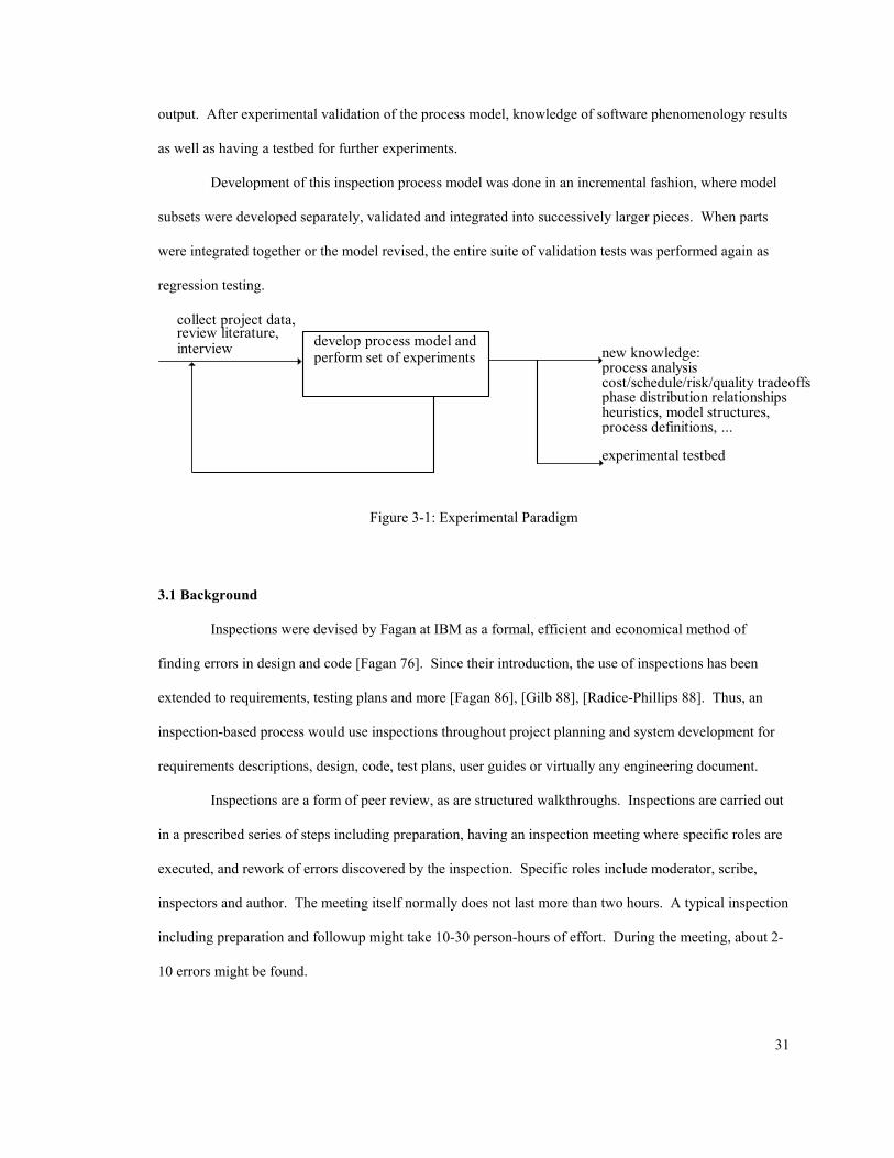
output. After experimental validation of the process model, knowledge of software phenomenology results

as well as having a testbed for further experiments.

Development of this inspection process model was done in an incremental fashion, where model

subsets were developed separately, validated and integrated into successively larger pieces. When parts

were integrated together or the model revised, the entire suite of validation tests was performed again as

regression testing.

develop process model andperform set of experiments

collect project data,review literature,interview new knowledge:

process analysiscost/schedule/risk/quality tradeoffsphase distribution relationshipsheuristics, model structures,process definitions, ...

experimental testbed

Figure 3-1: Experimental Paradigm

3.1 Background

Inspections were devised by Fagan at IBM as a formal, efficient and economical method of

finding errors in design and code [Fagan 76]. Since their introduction, the use of inspections has been

extended to requirements, testing plans and more [Fagan 86], [Gilb 88], [Radice-Phillips 88]. Thus, an

inspection-based process would use inspections throughout project planning and system development for

requirements descriptions, design, code, test plans, user guides or virtually any engineering document.

Inspections are a form of peer review, as are structured walkthroughs. Inspections are carried out

in a prescribed series of steps including preparation, having an inspection meeting where specific roles are

executed, and rework of errors discovered by the inspection. Specific roles include moderator, scribe,

inspectors and author. The meeting itself normally does not last more than two hours. A typical inspection

including preparation and followup might take 10-30 person-hours of effort. During the meeting, about 2-

10 errors might be found.

31

By detecting and correcting errors in earlier stages of the process such as design, significant cost

reductions can be made since the rework is much less costly compared to fixing errors later in the testing

and integration phases [Fagan 86], [Radice-Phillips 88], [Grady 92], [Madachy et al. 93a]. For instance,

only a couple hours are used to find a defect during an inspection but 5-20 hours might be required to fix it

during system test.

Authors have reported a wide range of inspection metrics. For example, guidelines for the proper

rates of preparation and inspection often differ geometrically as well as overall effectiveness (defects found

per person-hour). There have been simplistic static relationships published for net return-on-investment or

effort required as a function of pages or code, but none integrated together in a dynamic model. Neither do

any existing models provide guidelines for estimating inspection effort as a function of product size, or

estimating schedule when incorporating inspections.

In general, results have shown that extra effort is required during design and coding for

inspections and much more is saved during testing and integration. This reference behavioral effect is

shown in Figure 3.1-1 from [Fagan 86] that represents a goal of this modeling; to be able to demonstrate

this effect on effort and schedule as a function of inspection practices.

32

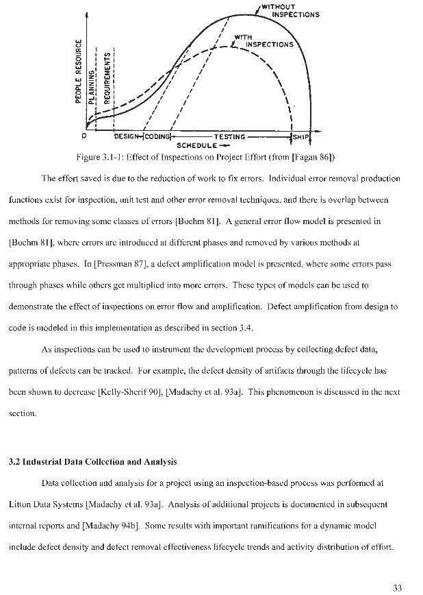
SCHEDULE - 1 1

Figure 3.1 - 1 : Effect of Inspections on Project Effort (from [Fagan 861)

The effort saved is due to the reduction of work to fix errors. Individual error removal production

functions exist for inspection, unit test and other error removal techniques, and there is overlap between

methods for removing some classes of errors [Boehm 811. A general error flow model is presented in

[Boehm 811, where errors are introduced at different phases and removed by various methods at

appropriate phases. In [Pressman 871, a defect amplification model is presented, where some errors pass

through phases while others get multiplied into more errors. These types of models can be used to

demonstrate the effect of inspections on error flow and amplification. Defect amplification from design to

code is modeled in this implementation as described in section 3.4.

As inspections can be used to instrument the development process by collecting defect data,

patterns of defects can be tracked. For example, the defect density of artifacts through the lifecycle has

been shown to decrease [Kelly-Sherif 901, [Madachy et al. 93al. This phenomenon is discussed in the next

section.

3.2 Industrial Data Collection and Analysis

Data collection and analysis for a project using an inspection-based process was performed at

Litton Data Systems [Madachy et al. 93al. Analysis of additional projects is documented in subsequent

internal reports and [Madachy 94bl. Some results with important ramifications for a dynamic model

include defect density and defect removal effectiveness lifecycle trends and activity distribution of effort.

Calibrations are made to match the model to these defect density trends and activity distributions in

selected test cases.

Data for the previous project at Litton in the same product line and having identical environmental

factors except for the use of inspections was also collected. It provides several parameters used in

development and calibration of the system dynamics model, and also enables a comparison to judge the

relative project effects from performing inspections.

Trouble report data from the project show an average defect density of about 48 defects/KSLOC

found during testing. The trouble report data also provides the average cost in person-hours to fix a defect

found during testing. This value is used for calculating the net return from inspections on the more recent

project.

When the defect densities for different document types are ordered by lifecycle activity, the

results show that the defects steadily decrease since the predecessor artifacts were previously inspected and

less defects are introduced as the project progresses. This is shown in Figure 3.2-1, overlayed with similar

results from JPL [Kelly-Sherif 90]. The trend corroborates the previous results. Code is not shown

because of inconsistencies in reporting the document size. These results strongly support the practice of

inspecting documents early as possible in the lifecycle, and can be used to calibrate defect rates for the

different development activities when inspection efficiency and page counts are known.

34

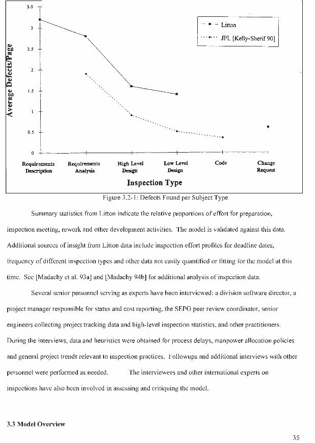
.-. * - - JPL, [Kelly-Sherif 901

Requirements Requirements High Level Low Level Code m e Dmiption m* - D&P Rrs-

Inspection Type

Figure 3.2-1: Defects Found per Subject Type

Summary statistics from Litton indicate the relative proportions of effort for preparation,

inspection meeting, rework and other development activities. The model is validated against this data.

Additional sources of insight from Litton data include inspection effort profiles for deadline dates,

frequency of different inspection types and other data not easily quantified or fitting for the model at this

time. See [Madachy et al. 93a] and [Madachy 94b] for additional analysis of inspection data.

Several senior personnel serving as experts have been interviewed: a division software director, a

project manager responsible for status and cost reporting, the SEPG peer review coordinator, senior

engineers collecting project tracking data and high-level inspection statistics, and other practitioners.

During the interviews, data and heuristics were obtained for process delays, manpower allocation policies

and general project trends relevant to inspection practices. Followups and additional interviews with other

personnel were performed as needed. The interviewees and other international experts on

inspections have also been involved in assessing and critiquing the model.

3.3 Model Overview

The model covers design through testing activities including inspections of design and code. It

assumes that inspections and system testing are the only defect removal activities, as practiced in a number

of organizations. It also assumes a team trained in inspections such that inspections can be inserted into the

process without associated training costs. Its staffing policy structure is based on mature software

organizations (SEI level 2 or above) that are fairly repeatable in terms of productivity such that the effect

of underestimation feedback does not play a major role in project behavior (though it could be incorporated

as such).

The ITHINK modeling package is used to implement the system dynamics method [Richmond et

al. 90]. It uses visual diagramming for constructing dynamic models, provides levels of abstraction, allows

for graphical representation of table functions and provides utilities for sophisticated model components

beyond previous implementations of system dynamics. Figure 3.4-1 is a diagram of the system dynamics

model of an inspection-based process. Source code for the model is provided in Appendix A.

36

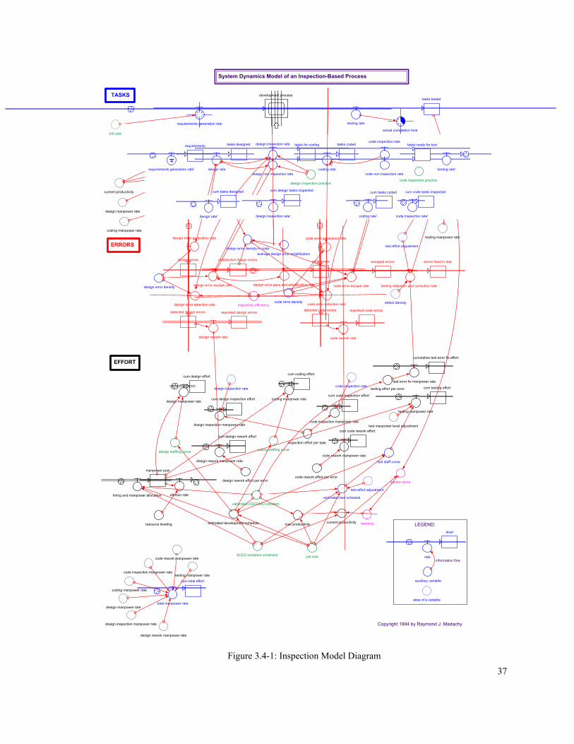
tasks tested

current productivity

~learning

job size

manpower pool

current productivity

~design staffing curve

resource leveling

fraction done

testing rate

cum code rework effort

max productivity

inspection effort per task

cum code inspection effort

code inspection manpower rate

code rework manpower rate

design rework effort per error

hiring and manpower allocation

cum design effort

design manpower rate

inspection efficiency

attrition rate

SCED schedule constraint

design inspection manpower rate

cum testing efforttesting effort per error

testing manpower rate

design manpower rate

job size

development process

requirements generation rate

code rework effort per error

calibrated COCOMO constant

average design error amplification

estimated development schedule

cumulative test error fix effort

~coding staffing curve

test error fix manpower rate

design inspection rate

cum coding effort

coding manpower rate

coding manpower rate

code inspection rate

design manpower rate

coding manpower rate

code inspection manpower ratetesting manpower rate

code rework manpower rate

cum design inspection effort

design inspection manpower rate

cum design rework effort

design rework manpower rate

cum total effort

total manpower rate

design rework manpower rate

level

rate

auxiliary variable

alias of a variable

actual completion time

estimated test schedule

~test staff curve

testing manpower rate

test effort adjustment

test effort adjustment

test manpower level adjustment

design error density

defect density

design error density in code

code error density

TASKS

EFFORT

LEGEND:

information flow

Copyright 1994 by Raymond J. Madachy

System Dynamics Model of an Inspection-Based Process

requirements

requirements generation rate'

cum tasks designed

tasks designed

design rate

design rate'

design non inspection rate

tasks for codingdesign inspection rate

cum design tasks inspected

design inspection rate'

tasks coded

coding rate

code inspection rate

code non inspection rate

cum tasks coded

coding rate'

design inspection practice

testing rate'

tasks ready for test

code inspection practice

cum code tasks inspected

code inspection rate'

design errors code errors

detected design errors

design error generation rate

design error escape rate

design error detection rate

design rework rate

reworked design errors

undetected design errors errors fixed in test

design error pass and amplification rate

code error generation rate

detected code errors

code error detection rate

reworked code errors

code rework rate

escaped errors

code error escape rate testing detection and correction rate

ERRORS

Figure 3.4-1: Inspection Model Diagram 37

Project behavior is initiated with the influx of requirements. Rates for the different phase

activities are constrained by the manpower allocations and current productivity, and are integrated to

determine the state variables, or levels of tasks in design, code, inspection, testing, etc. The tasks are either

inspected or not during design or code activities as a function of inspection practices.

Errors are generated as a co-flow of design and coding activities, and eventually detected by

inspections or passed onto the next phase. The detection of errors is a function of inspection practices and

inspection efficiency. All errors detected during inspections are then reworked. Note that escaped design

errors are amplified into coding errors. Those errors that still escape code inspections are then detected and

corrected during integration and test activities. The effort and schedule for the testing phase is adjusted for

the remaining error levels.

Other sectors of the model implement management policies such as allocating personnel resources

and defining staffing curves for the different activities. Input to the policy decisions are the job size,

productivity, schedule constraints and resource leveling constraints. Effort is instrumented in a cumulative

fashion for all of the defined activities. Learning takes place as a function of the job completion, and

adjusts the productivity. Schedule compression effects are approximated similar to the COCOMO cost

driver effects for relative schedule.

The actual completion time is implemented as a cycle time utility whose final value represents the

actual schedule. It instruments the maximum in-process time of the tasks that are time-stamped at

requirements generation rate and complete testing.

Correspondence between the dynamic model and COCOMO is illustrated in Figure 3.4-2. It is

based on the phase effort and schedule of a 32 KSLOC embedded mode reference project. For the nominal

case of no inspections performed, the manpower allocation policy employs the curves to match the

rectangular COCOMO effort profiles as a calibration between the models. Thus the area under the design

curve matches the aggregated COCOMO preliminary and detailed design, and likewise for the coding and

testing curves.

38

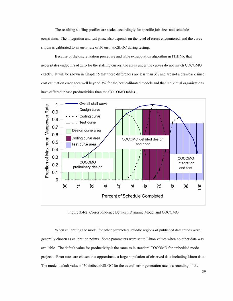
The resulting staffing profiles are scaled accordingly for specific job sizes and schedule

constraints. The integration and test phase also depends on the level of errors encountered, and the curve

shown is calibrated to an error rate of 50 errors/KSLOC during testing.

Because of the discretization procedure and table extrapolation algorithm in ITHINK that

necessitates endpoints of zero for the staffing curves, the areas under the curves do not match COCOMO

exactly. It will be shown in Chapter 5 that these differences are less than 3% and are not a drawback since

cost estimation error goes well beyond 3% for the best calibrated models and that individual organizations

have different phase productivities than the COCOMO tables.

0

0.1

0.2

0.3

0.4

0.5

0.6

0.7

0.8

0.9

1

00 10 20 30 40 50 60 70 80 90 100

Percent of Schedule Completed

Frac

tion

of M

axim

um M

anpo

wer

Rat

e

Design curve area

Coding curve area COCOMO detailed design and code

COCOMO integration and test

COCOMO preliminary design

Test curve area

Design curve

Coding curve

Test curve

Overall staff curve

Figure 3.4-2: Correspondence Between Dynamic Model and COCOMO

When calibrating the model for other parameters, middle regions of published data trends were

generally chosen as calibration points. Some parameters were set to Litton values when no other data was

available. The default value for productivity is the same as in standard COCOMO for embedded mode

projects. Error rates are chosen that approximate a large population of observed data including Litton data.

The model default value of 50 defects/KSLOC for the overall error generation rate is a rounding of the 39

Litton value of 48 defects/KSLOC. Included in the demonstration cases in Chapter 5 are model

calibrations for specific project instances.

Per the experience at Litton and accordant with other published data, inspection effort that

includes preparation, meeting and rework generally consumes approximately 5-10% of total project effort.

Guidelines for inspection rates are always stated as linear with the number of pages (or lines of code), and

the inspection effort is set accordingly in the model. That is, inspection effort does not exhibit diseconomy

of scale as total project effort does in COCOMO and most other cost models. The default inspection effort

also corresponds to a rate of 250 LOC/hour during preparation and inspection with an average of four

inspectors per meeting [Grady 92].

The rework effort per error found in inspection is set differently for design and code. Litton data

shows that the average cost to rework an error during code is about 1.3 times that for design. The cost to

fix errors from [Boehm 81] shows that the relative cost for code is twice that of design. The model is set at

this 2:1 ratio since it is based on a larger set of data. The resulting values are also close to the reported

ranges of published data from JPL [Kelly-Sherif 90]. The testing fixing effort per error is set at about 5

hours, which is well within the range of reported metrics. The inspection efficiency is nominally set at .6,

representing the fraction of defects found through inspections. Reported rates vary from about 50% to

90% of defects found.

The utility of the model for a particular organization is dependent on calibrating it accordingly per

local data. While model parameters are set with reasonable numbers to investigate inspections in general,

the results using the defaults will not necessarily reflect all environments. Besides the efficiency and effort

of inspections, differing project environments could have far different error rates, rework effort, testing

effort or documentation sizes.

The model is completely original, though it can be compared to previous research. Using the

system dynamics model in [Abdel-Hamid-Madnick 91] as a conceptual reference baseline, this inspection-

based process model replaces the software production, quality assurance (QA) and system testing sectors.

The model boundaries for this work are shown against a highly aggregated view of Abdel-Hamid’s model

in Figure 3.4-3. The boundary is drawn so that schedule pressure effects, personnel mix, and other coding

40

productivity determinants do not confound the inspection analysis.

41

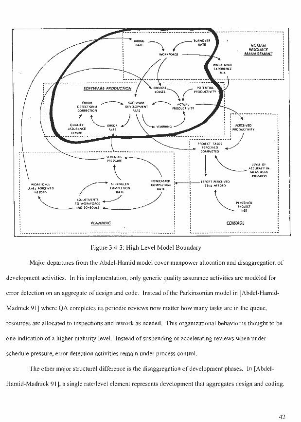
Major departures from the Abdel-Hamid model cover manpower allocation and disaggregation of

development activities. In his implementation, only generic quality assurance activities are modeled for

error detection on an aggregate of design and code. Instead of the Parkinsonian model in [Abdel-Hamid-

Madnick 9 11 where QA completes its periodic reviews now matter how many tasks are in the queue,

resources are allocated to inspections and rework as needed. This organizational behavior is thought to be

one indication of a higher maturity level. Instead of suspending or accelerating reviews when under

schedule pressure, error detection activities remain under process control.

The other major structural difference is the disaggregation of development phases. In [Abdel-

Hamid-Madnick 911, a single ratellevel element represents development that aggregates design and coding.

In this formulation, activities are delineated and decomposed corresponding to the phases defined in the

COCOMO model. Design and coding are modeled independently.

See Appendix A System Dynamics Model Supplement for further descriptions of the model

including source code, reference behavior charts and description, test case results, and summary results of

the validation tests.

43

Chapter 4 Knowledge-Based Risk Assessment and Cost Estimation

This chapter describes the development and usage of a method for providing knowledge-based

assistance for software project risk management and cost estimation.

4.1 Background The objective of software risk management is to identify, address and eliminate risk items before

undesirable outcomes occur. Its practice can be improved by leveraging on existing knowledge and

expertise. In particular, expert knowledge can be employed during cost estimation activities by using cost

factors for risk identification and assessment to detect patterns of project risk.

During cost estimation, consistency constraints and cost model assumptions may be violated or an

estimator may overlook project planning discrepancies and fail to realize risks. Approaches for identifying

risks are usually separate from cost estimation, thus a technique that identifies risk in conjunction with cost

estimation is an improvement.

COCOMO is a widely used cost model that incorporates the use of cost drivers to adjust effort

calculations. As significant project factors, cost drivers can be used for risk assessment using sensitivity

analysis or Monte-Carlo simulation, but this approach uses them to infer specific risk situations.

Mitre developed an Expert System Cost Model (ESCOMO) employing an expert system shell on a

PC [Day 87]. It used 46 rules involving COCOMO cost drivers and other model inputs to focus on input

anomalies and consistency checks with no quantitative risk assessment.

4.2 Method

Knowledge was acquired from written sources on cost estimation [Boehm 81, Boehm-Royce 89,

Day 87], risk management [Boehm 89, Charette 89] and domain experts including Dr. Barry Boehm,

Walker Royce and this author.

A matrix of COCOMO cost drivers was used as a starting point for identifying risk situations as a

combination of multiple cost attributes, and the risks were formulated into a set of rules. As such, the risk

44

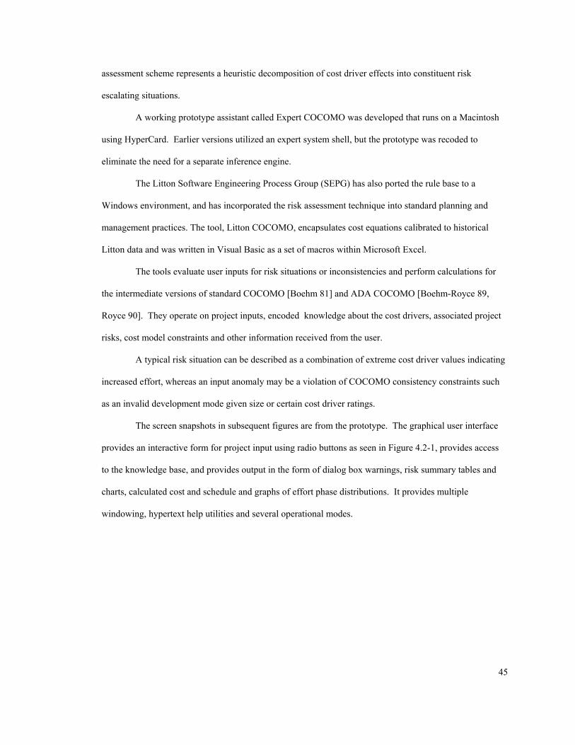
assessment scheme represents a heuristic decomposition of cost driver effects into constituent risk

escalating situations.

A working prototype assistant called Expert COCOMO was developed that runs on a Macintosh

using HyperCard. Earlier versions utilized an expert system shell, but the prototype was recoded to

eliminate the need for a separate inference engine.

The Litton Software Engineering Process Group (SEPG) has also ported the rule base to a

Windows environment, and has incorporated the risk assessment technique into standard planning and

management practices. The tool, Litton COCOMO, encapsulates cost equations calibrated to historical

Litton data and was written in Visual Basic as a set of macros within Microsoft Excel.

The tools evaluate user inputs for risk situations or inconsistencies and perform calculations for

the intermediate versions of standard COCOMO [Boehm 81] and ADA COCOMO [Boehm-Royce 89,

Royce 90]. They operate on project inputs, encoded knowledge about the cost drivers, associated project

risks, cost model constraints and other information received from the user.

A typical risk situation can be described as a combination of extreme cost driver values indicating

increased effort, whereas an input anomaly may be a violation of COCOMO consistency constraints such

as an invalid development mode given size or certain cost driver ratings.

The screen snapshots in subsequent figures are from the prototype. The graphical user interface

provides an interactive form for project input using radio buttons as seen in Figure 4.2-1, provides access

to the knowledge base, and provides output in the form of dialog box warnings, risk summary tables and

charts, calculated cost and schedule and graphs of effort phase distributions. It provides multiple

windowing, hypertext help utilities and several operational modes.

45

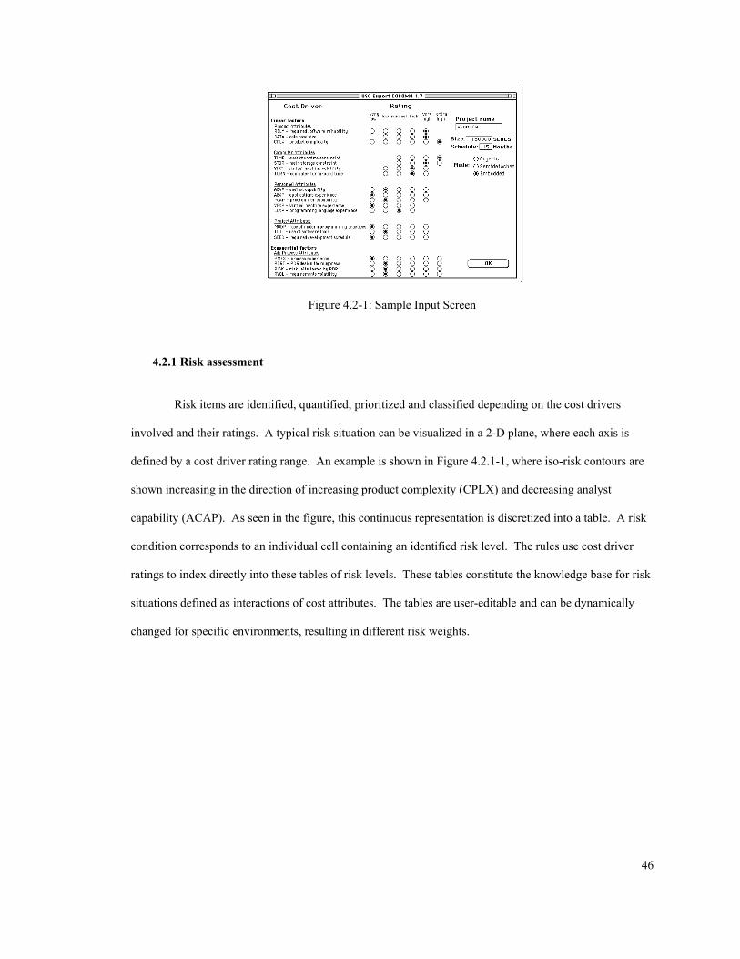
Figure 4.2-1: Sample Input Screen

4.2.1 Risk assessment

Risk items are identified, quantified, prioritized and classified depending on the cost drivers

involved and their ratings. A typical risk situation can be visualized in a 2-D plane, where each axis is

defined by a cost driver rating range. An example is shown in Figure 4.2.1-1, where iso-risk contours are

shown increasing in the direction of increasing product complexity (CPLX) and decreasing analyst

capability (ACAP). As seen in the figure, this continuous representation is discretized into a table. A risk

condition corresponds to an individual cell containing an identified risk level. The rules use cost driver

ratings to index directly into these tables of risk levels. These tables constitute the knowledge base for risk

situations defined as interactions of cost attributes. The tables are user-editable and can be dynamically

changed for specific environments, resulting in different risk weights.

46

very low CPLX extra high

very low very high high ACAP moderate very high discretized into

CPLX ACAP HIGH VERY HIGH EXTRA

HIGH VERY LOW MODERATE HIGH VERY HIGH LOW MODERATE HIGH NOMINAL MODERATE

Figure 4.2.1-1: Assignment of Risk Levels

In order to categorize the risks, a risk taxonomy was developed by analyzing the proposed rule

base with respect to existing COCOMO cost attribute categories and other attributes deemed important to

risk assessment. The cost drivers in COCOMO are grouped into product, computer, personnel, and project

categories. The project attributes were redesignated as process attributes, and ADA COCOMO process

factors have also been included in the process category. The resulting project risk categories are schedule,

product, personnel, process and computer. Input anomaly rules identify another type of risk where cost

model constraints or consistency checks are violated; a cost estimation risk of a poorly done estimate.

After several iterations of the prototype, the experts were engaged again to help quantify the risks.

A quantitative risk weighting scheme was developed that accounts for the nonlinearity of the assigned risk

levels and cost multiplier data to compute overall risks for each category and the entire project according to

project risk

risk level

effort multiplier product ,

=

==∑∑ i ji

category risks

j

categories

i j

, *##

11

47

where risk level = 1 moderate

2 high

4 very high

effort multiplier product=

(driver #1 effort multiplier) *

(driver #2 effort multiplier) ... *

(driver #n effort multiplier).

If the risk involves a schedule constraint (SCED), then

effort multiplier product=

(SCED effort multiplier)/(relative schedule)*

(driver #2 effort multiplier)...*

(driver #n effort multiplier).

The risk level corresponds to the probability of the risk occurring and the effort multiplier product

represents the cost consequence of the risk. The product involves those effort multipliers involved in the

risk situation. When the risk involves a schedule constraint, the product is divided by the relative schedule

to obtain the change in the average personnel level (the near-term cost) since the staffing profile is

compressed into a shorter project time. The risk assessment calculates general project risks, indicating a

probability of not meeting cost, schedule or performance goals.

The risk levels need normalization to provide meaningful relative risk indications. Sensitivity

analysis was performed to determine the sensitivity of the quantified risks with varying inputs, and extreme

conditions were tested. An initial scale with benchmarks for low, medium and high overall project risk

was developed as follows: 0-15 low risk, 15-50 medium risk, 50-350 high risk.

The individual risks are also ranked, and the different risk summaries are presented in a set of

tables. An example risk output is seen in Figure 4.2.1-2, showing the overall project risk and risks for

subcategories. This example is for an extremely risky project, where many cost drivers are rated at their

costliest values. The interface supports embedded hypertext links, so the user can click on a risk item in a

list to traverse to a screen containing the associated risk table and related information. Other outputs 48

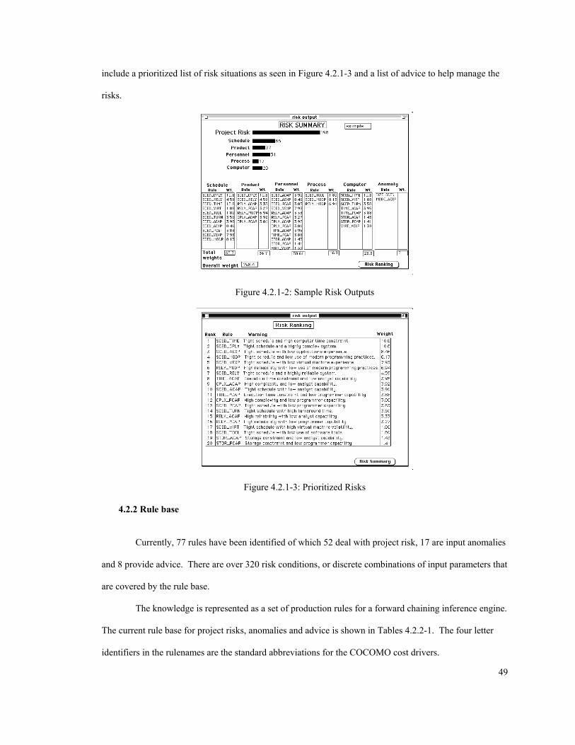
include a prioritized list of risk situations as seen in Figure 4.2.1-3 and a list of advice to help manage the

risks.

Figure 4.2.1-2: Sample Risk Outputs

Figure 4.2.1-3: Prioritized Risks

4.2.2 Rule base

Currently, 77 rules have been identified of which 52 deal with project risk, 17 are input anomalies

and 8 provide advice. There are over 320 risk conditions, or discrete combinations of input parameters that

are covered by the rule base.

The knowledge is represented as a set of production rules for a forward chaining inference engine.

The current rule base for project risks, anomalies and advice is shown in Tables 4.2.2-1. The four letter

identifiers in the rulenames are the standard abbreviations for the COCOMO cost drivers.

49

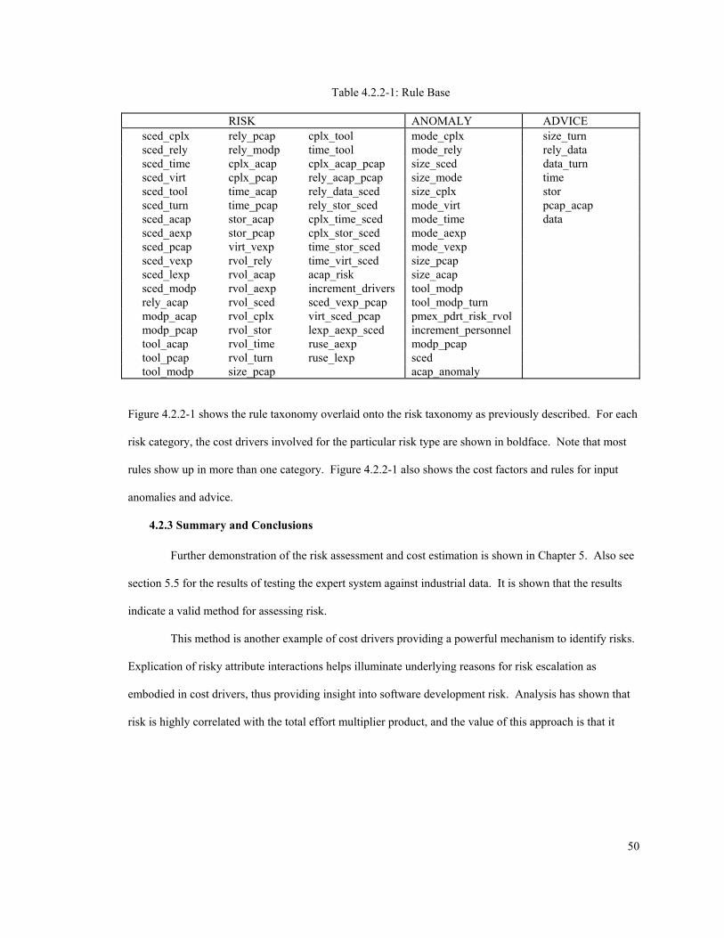
Table 4.2.2-1: Rule Base

RISK ANOMALY ADVICE sced_cplx rely_pcap cplx_tool mode_cplx size_turn sced_rely rely_modp time_tool mode_rely rely_data sced_time cplx_acap cplx_acap_pcap size_sced data_turn sced_virt cplx_pcap rely_acap_pcap size_mode time sced_tool time_acap rely_data_sced size_cplx stor sced_turn time_pcap rely_stor_sced mode_virt pcap_acap sced_acap stor_acap cplx_time_sced mode_time data sced_aexp stor_pcap cplx_stor_sced mode_aexp sced_pcap virt_vexp time_stor_sced mode_vexp sced_vexp rvol_rely time_virt_sced size_pcap sced_lexp rvol_acap acap_risk size_acap sced_modp rvol_aexp increment_drivers tool_modp rely_acap rvol_sced sced_vexp_pcap tool_modp_turn modp_acap rvol_cplx virt_sced_pcap pmex_pdrt_risk_rvol modp_pcap rvol_stor lexp_aexp_sced increment_personnel tool_acap rvol_time ruse_aexp modp_pcap tool_pcap rvol_turn ruse_lexp sced tool_modp size_pcap acap_anomaly

Figure 4.2.2-1 shows the rule taxonomy overlaid onto the risk taxonomy as previously described. For each

risk category, the cost drivers involved for the particular risk type are shown in boldface. Note that most

rules show up in more than one category. Figure 4.2.2-1 also shows the cost factors and rules for input

anomalies and advice.

4.2.3 Summary and Conclusions Further demonstration of the risk assessment and cost estimation is shown in Chapter 5. Also see

section 5.5 for the results of testing the expert system against industrial data. It is shown that the results

indicate a valid method for assessing risk.

This method is another example of cost drivers providing a powerful mechanism to identify risks.

Explication of risky attribute interactions helps illuminate underlying reasons for risk escalation as

embodied in cost drivers, thus providing insight into software development risk. Analysis has shown that

risk is highly correlated with the total effort multiplier product, and the value of this approach is that it

50

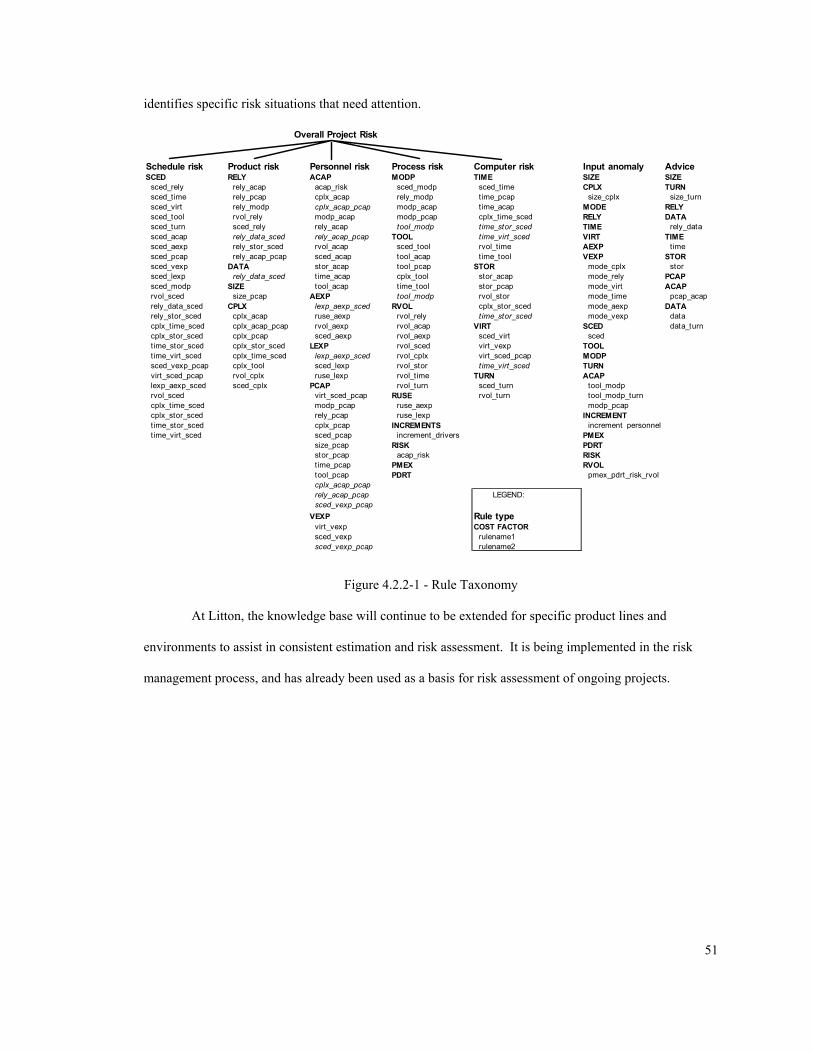
identifies specific risk situations that need attention.

Overall Project Risk

Schedule risk Product risk Personnel risk Process risk Computer risk Input anomaly AdviceSCED RELY ACAP MODP TIME SIZE SIZE sced_rely rely_acap acap_risk sced_modp sced_time CPLX TURN sced_time rely_pcap cplx_acap rely_modp t ime_pcap size_cplx size_turn sced_virt rely_modp cplx_acap_pcap modp_acap t ime_acap MODE RELY sced_tool rvol_rely modp_acap modp_pcap cplx_time_sced RELY DATA sced_turn sced_rely rely_acap tool_modp t ime_stor_sced TIME rely_data sced_acap rely_data_sced rely_acap_pcap TOOL t ime_virt_sced VIRT TIME sced_aexp rely_stor_sced rvol_acap sced_tool rvol_time AEXP t ime sced_pcap rely_acap_pcap sced_acap tool_acap t ime_tool VEXP STOR sced_vexp DATA stor_acap tool_pcap STOR mode_cplx stor sced_lexp rely_data_sced t ime_acap cplx_tool stor_acap mode_rely PCAP sced_modp SIZE tool_acap time_tool stor_pcap mode_virt ACAP rvol_sced size_pcap AEXP tool_modp rvol_stor mode_time pcap_acap rely_data_sced CPLX lexp_aexp_sced RVOL cplx_stor_sced mode_aexp DATA rely_stor_sced cplx_acap ruse_aexp rvol_rely t ime_stor_sced mode_vexp data cplx_time_sced cplx_acap_pcap rvol_aexp rvol_acap VIRT SCED data_turn cplx_stor_sced cplx_pcap sced_aexp rvol_aexp sced_virt sced time_stor_sced cplx_stor_sced LEXP rvol_sced virt_vexp TOOL time_virt_sced cplx_time_sced lexp_aexp_sced rvol_cplx virt_sced_pcap MODP sced_vexp_pcap cplx_tool sced_lexp rvol_stor t ime_virt_sced TURN virt_sced_pcap rvol_cplx ruse_lexp rvol_time TURN ACAP lexp_aexp_sced sced_cplx PCAP rvol_turn sced_turn tool_modp rvol_sced virt_sced_pcap RUSE rvol_turn tool_modp_turn cplx_time_sced modp_pcap ruse_aexp modp_pcap cplx_stor_sced rely_pcap ruse_lexp INCREMENT time_stor_sced cplx_pcap INCREMENTS increment personnel time_virt_sced sced_pcap increment_drivers PMEX

size_pcap RISK PDRT stor_pcap acap_risk RISK t ime_pcap PMEX RVOL tool_pcap PDRT pmex_pdrt_risk_rvol cplx_acap_pcap rely_acap_pcap LEGEND: sced_vexp_pcapVEXP Rule type virt_vexp COST FACTOR sced_vexp rulename1 sced_vexp_pcap rulename2

Figure 4.2.2-1 - Rule Taxonomy

At Litton, the knowledge base will continue to be extended for specific product lines and

environments to assist in consistent estimation and risk assessment. It is being implemented in the risk

management process, and has already been used as a basis for risk assessment of ongoing projects.

51

Chapter 5 Model Demonstration and Evaluation

This chapter shows how the model is tested with various sets of test cases and industrial data, and

demonstrates use of the model for several managerial purposes. Results of the simulation runs and risk

assessments are evaluated from several perspectives and insights are provided by experimenting with the

model.

Model validation in system dynamics extends quantitative validation with an extensive range and

depth of qualitative criteria. The emphasis is on building confidence in the suitability of the model for its

intended purposes and its consistency with observed reality [Richardson 91]. A summary of validation

tests is shown in Table 5-1, which is adapted from [Richardson 81] and [Forrester-Senge 80]. For each

test, the number, name and passing criteria are identified. The criteria for a valid model consist of the tests

in this table and associated subtests. Each individual test is insufficient alone to validate a model, but taken

together they provide a robust means of filtering out weak models.

The battery of tests in Table 5-1 considers the model’s suitability for purpose, consistency with

reality, and utility and effectiveness from both structural and behavioral perspectives. Specific modeling

objectives to test against include the ability to predict design and code effort sans inspection, preparation

and inspection meeting effort, rework effort, testing effort, schedule and error levels as a function of

development phase. Simulation test case results are compared against collected data and other published

data, existing theory and other prediction models. Testing includes examining the ability of the model to

generate proper reference behavior, which consists of time histories for all model variables.

52

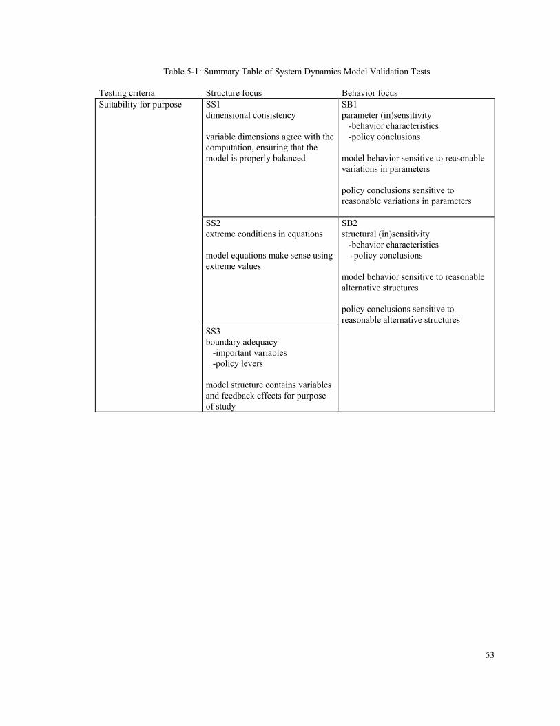
Table 5-1: Summary Table of System Dynamics Model Validation Tests

Testing criteria Structure focus Behavior focus Suitability for purpose SS1

dimensional consistency variable dimensions agree with the computation, ensuring that the model is properly balanced

SB1 parameter (in)sensitivity -behavior characteristics -policy conclusions model behavior sensitive to reasonable variations in parameters policy conclusions sensitive to reasonable variations in parameters

SS2 extreme conditions in equations model equations make sense using extreme values

SB2 structural (in)sensitivity -behavior characteristics -policy conclusions model behavior sensitive to reasonable alternative structures policy conclusions sensitive to reasonable alternative structures

SS3 boundary adequacy -important variables -policy levers model structure contains variables and feedback effects for purpose of study

53

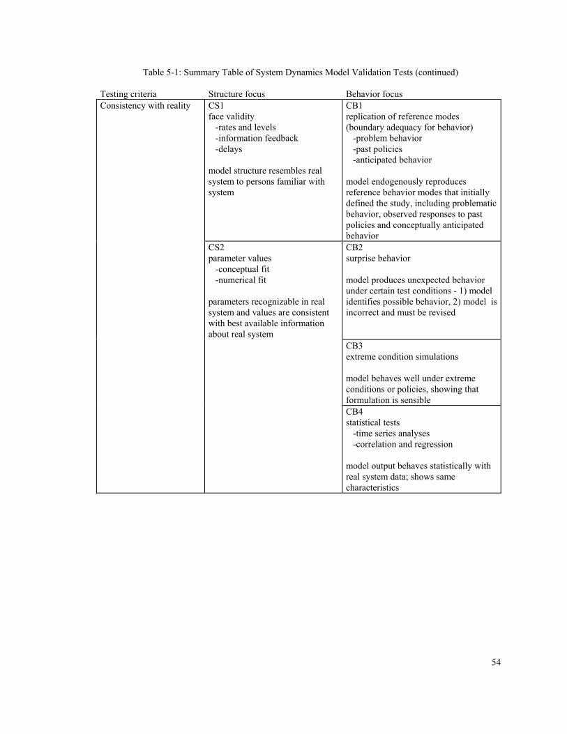
Table 5-1: Summary Table of System Dynamics Model Validation Tests (continued)

Testing criteria Structure focus Behavior focus Consistency with reality CS1

face validity -rates and levels -information feedback -delays model structure resembles real system to persons familiar with system

CB1 replication of reference modes (boundary adequacy for behavior) -problem behavior -past policies -anticipated behavior model endogenously reproduces reference behavior modes that initially defined the study, including problematic behavior, observed responses to past policies and conceptually anticipated behavior

CS2 parameter values -conceptual fit -numerical fit parameters recognizable in real system and values are consistent with best available information about real system

CB2 surprise behavior model produces unexpected behavior under certain test conditions - 1) model identifies possible behavior, 2) model is incorrect and must be revised

CB3 extreme condition simulations model behaves well under extreme conditions or policies, showing that formulation is sensible

CB4 statistical tests -time series analyses -correlation and regression model output behaves statistically with real system data; shows same characteristics

54

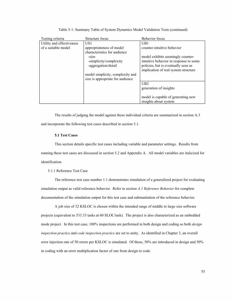
Table 5-1: Summary Table of System Dynamics Model Validation Tests (continued)

Testing criteria Structure focus Behavior focus Utility and effectiveness of a suitable model

US1 appropriateness of model characteristics for audience -size -simplicity/complexity -aggregation/detail model simplicity, complexity and size is appropriate for audience

UB1 counter-intuitive behavior model exhibits seemingly counter-intuitive behavior in response to some policies, but is eventually seen as implication of real system structure

UB2 generation of insights model is capable of generating new insights about system

The results of judging the model against these individual criteria are summarized in section A.3

and incorporate the following test cases described in section 5.1.

5.1 Test Cases

This section details specific test cases including variable and parameter settings. Results from

running these test cases are discussed in section 5.2 and Appendix A. All model variables are italicized for

identification.

5.1.1 Reference Test Case

The reference test case number 1.1 demonstrates simulation of a generalized project for evaluating

simulation output as valid reference behavior. Refer to section A.1 Reference Behavior for complete

documentation of the simulation output for this test case and substantiation of the reference behavior.

A job size of 32 KSLOC is chosen within the intended range of middle to large size software

projects (equivalent to 533.33 tasks at 60 SLOC/task). The project is also characterized as an embedded

mode project. In this test case, 100% inspections are performed in both design and coding so both design

inspection practice and code inspection practice are set to unity. As identified in Chapter 3, an overall

error injection rate of 50 errors per KSLOC is simulated. Of those, 50% are introduced in design and 50%

in coding with an error multiplication factor of one from design to code.

55

Certain other parameters in the model need to be calibrated for specific project situations, and the

following subsection provides direction for doing so using this test case as an example.

5.1.1.1 Calibration Procedure

Each modeled project should have productivity, error rates, rework effort parameters, test error

fixing effort and inspection factors calibrated for the particular environment. Some hardwired model

defaults include phase productivity proportions for design and coding, and schedule proportions for phase

activities as illustrated in Figure 3.4-2 and further documented in section A.4 in the equations.

The calibrated COCOMO constant parameter represents an organizational productivity factor

whose magnitude is determined through project data collection and analysis. It is the leading constant in

the COCOMO effort equations. The default value of 3.6 for the embedded mode is used in this test case.

The error density of 50 errors/KSLOC is equivalent to 3 total errors per task distributed evenly

between design and coding, so design error density is set at 1.5 and code error density is set at 1.5 in the

model.

The parameters design rework effort per error and code rework effort per error are set at .055 and

.11 person-days respectively (.44 and .88 person-hours), according to the parameter setting described in

Chapter 3. The test error fixing effort is set at 4.6 person-hours with testing effort per error by

appropriately setting the multiplier of the calibrated COCOMO constant. The inspection efficiency is

nominally set at .6 as stated in Chapter 3. Both design inspection practice and code inspection practice are

set to one, indicating 100% inspections are performed.

5.1.2 Additional Test Cases

Table 5.1.2-1 identifies sets of test cases, the factors investigated and model parameters that are

varied for the simulation. Settings for the parameters in individual test cases are shown in the other

sections of this chapter accompanied with the results of the specific simulation experiments. A complete

list of test case results are shown in section A.2.

56

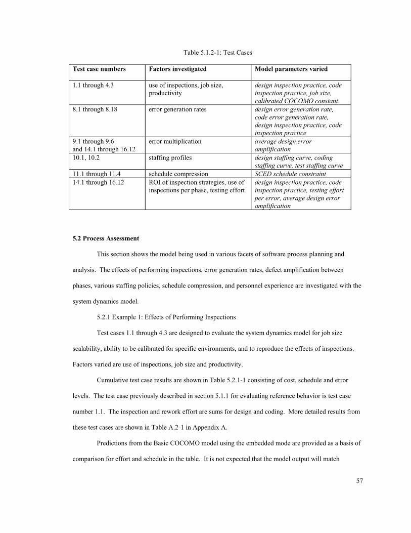
Table 5.1.2-1: Test Cases

Test case numbers Factors investigated Model parameters varied

1.1 through 4.3 use of inspections, job size, productivity

design inspection practice, code inspection practice, job size, calibrated COCOMO constant

8.1 through 8.18 error generation rates design error generation rate, code error generation rate, design inspection practice, code inspection practice

9.1 through 9.6 and 14.1 through 16.12

error multiplication average design error amplification

10.1, 10.2 staffing profiles design staffing curve, coding staffing curve, test staffing curve

11.1 through 11.4 schedule compression SCED schedule constraint 14.1 through 16.12 ROI of inspection strategies, use of

inspections per phase, testing effort design inspection practice, code inspection practice, testing effort per error, average design error amplification

5.2 Process Assessment

This section shows the model being used in various facets of software process planning and

analysis. The effects of performing inspections, error generation rates, defect amplification between

phases, various staffing policies, schedule compression, and personnel experience are investigated with the

system dynamics model.

5.2.1 Example 1: Effects of Performing Inspections

Test cases 1.1 through 4.3 are designed to evaluate the system dynamics model for job size

scalability, ability to be calibrated for specific environments, and to reproduce the effects of inspections.

Factors varied are use of inspections, job size and productivity.

Cumulative test case results are shown in Table 5.2.1-1 consisting of cost, schedule and error

levels. The test case previously described in section 5.1.1 for evaluating reference behavior is test case

number 1.1. The inspection and rework effort are sums for design and coding. More detailed results from

these test cases are shown in Table A.2-1 in Appendix A.

Predictions from the Basic COCOMO model using the embedded mode are provided as a basis of

comparison for effort and schedule in the table. It is not expected that the model output will match

57

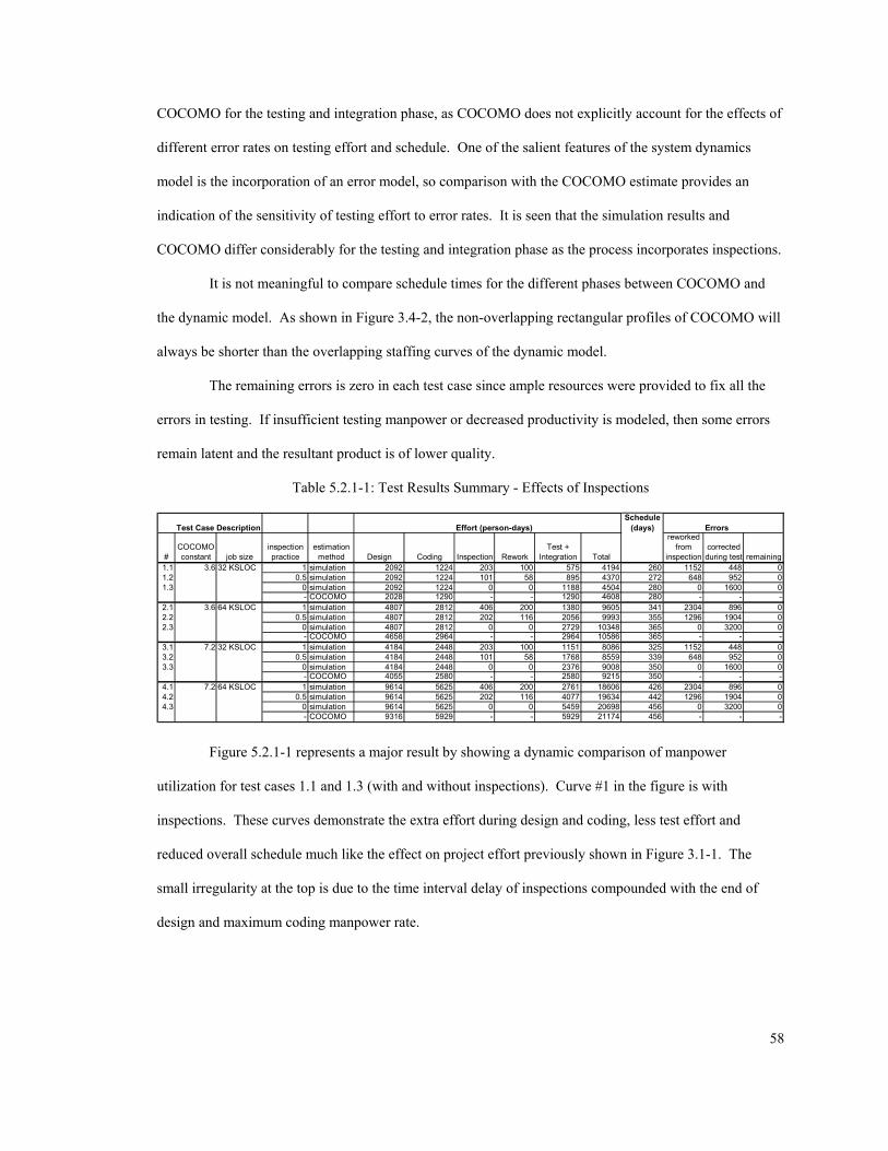
COCOMO for the testing and integration phase, as COCOMO does not explicitly account for the effects of

different error rates on testing effort and schedule. One of the salient features of the system dynamics

model is the incorporation of an error model, so comparison with the COCOMO estimate provides an

indication of the sensitivity of testing effort to error rates. It is seen that the simulation results and

COCOMO differ considerably for the testing and integration phase as the process incorporates inspections.

It is not meaningful to compare schedule times for the different phases between COCOMO and

the dynamic model. As shown in Figure 3.4-2, the non-overlapping rectangular profiles of COCOMO will

always be shorter than the overlapping staffing curves of the dynamic model.

The remaining errors is zero in each test case since ample resources were provided to fix all the

errors in testing. If insufficient testing manpower or decreased productivity is modeled, then some errors

remain latent and the resultant product is of lower quality.

Table 5.2.1-1: Test Results Summary - Effects of Inspections

Test Case Description Effort (person-days)Schedule

(days) Errors

#COCOMO constant job size

inspection practice

estimation method Design Coding Inspection Rework

Test + Integration Total

reworked from

inspectioncorrected during test remaining

1.1 3.6 32 KSLOC 1 simulation 2092 1224 203 100 575 4194 260 1152 448 01.2 0.5 simulation 2092 1224 101 58 895 4370 272 648 952 01.3 0 simulation 2092 1224 0 0 1188 4504 280 0 1600 0

- COCOMO 2028 1290 - - 1290 4608 280 - - -2.1 3.6 64 KSLOC 1 simulation 4807 2812 406 200 1380 9605 341 2304 896 02.2 0.5 simulation 4807 2812 202 116 2056 9993 355 1296 1904 02.3 0 simulation 4807 2812 0 0 2729 10348 365 0 3200 0

- COCOMO 4658 2964 - - 2964 10586 365 - - -3.1 7.2 32 KSLOC 1 simulation 4184 2448 203 100 1151 8086 325 1152 448 03.2 0.5 simulation 4184 2448 101 58 1768 8559 339 648 952 03.3 0 simulation 4184 2448 0 0 2376 9008 350 0 1600 0

- COCOMO 4055 2580 - - 2580 9215 350 - - -4.1 7.2 64 KSLOC 1 simulation 9614 5625 406 200 2761 18606 426 2304 896 04.2 0.5 simulation 9614 5625 202 116 4077 19634 442 1296 1904 04.3 0 simulation 9614 5625 0 0 5459 20698 456 0 3200 0

- COCOMO 9316 5929 - - 5929 21174 456 - - -

Figure 5.2.1-1 represents a major result by showing a dynamic comparison of manpower

utilization for test cases 1.1 and 1.3 (with and without inspections). Curve #1 in the figure is with

inspections. These curves demonstrate the extra effort during design and coding, less test effort and

reduced overall schedule much like the effect on project effort previously shown in Figure 3.1-1. The

small irregularity at the top is due to the time interval delay of inspections compounded with the end of

design and maximum coding manpower rate.

58

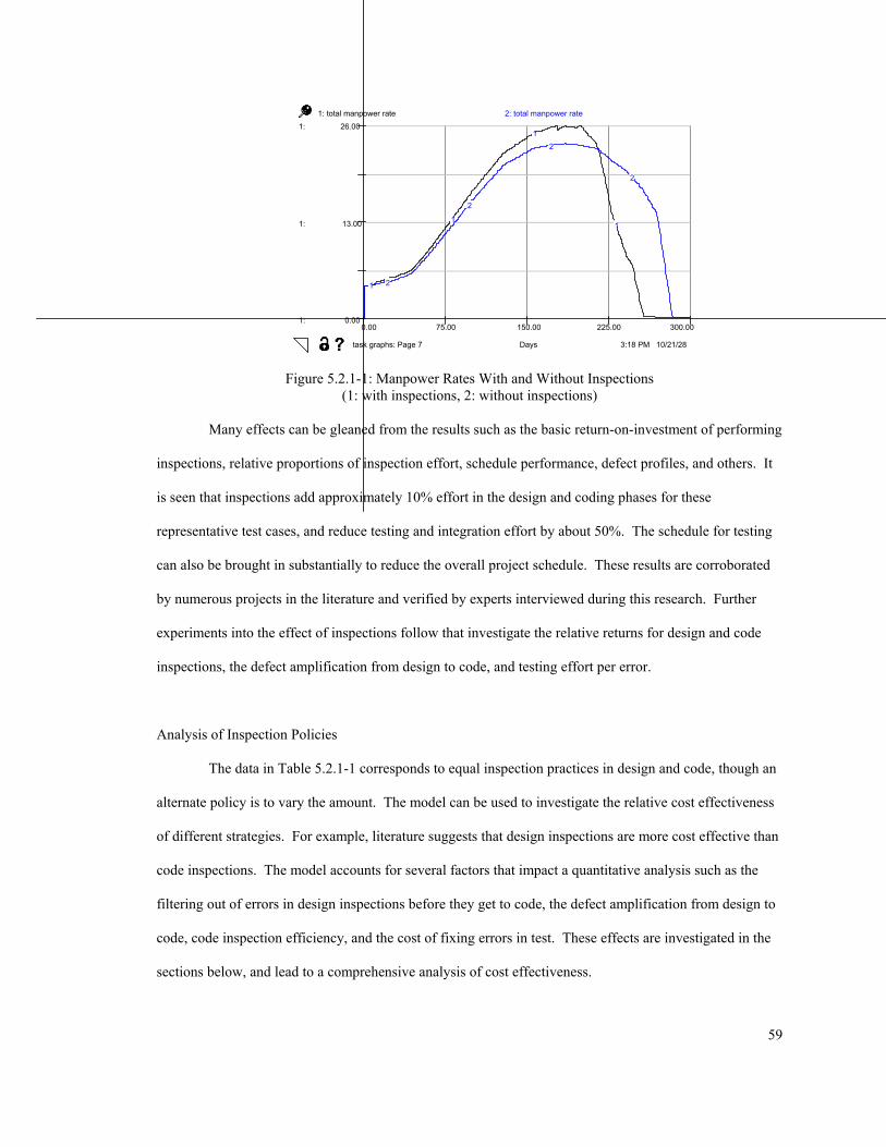
3:18 PM 10/21/28

0.00 75.00 150.00 225.00 300.00

Days

1:

1:

1:

0.00

13.00

26.00

1: total manpower rate 2: total manpower rate

1

1

1

1

2

2

2

2

task graphs: Page 7

Figure 5.2.1-1: Manpower Rates With and Without Inspections (1: with inspections, 2: without inspections)

Many effects can be gleaned from the results such as the basic return-on-investment of performing

inspections, relative proportions of inspection effort, schedule performance, defect profiles, and others. It

is seen that inspections add approximately 10% effort in the design and coding phases for these

representative test cases, and reduce testing and integration effort by about 50%. The schedule for testing

can also be brought in substantially to reduce the overall project schedule. These results are corroborated

by numerous projects in the literature and verified by experts interviewed during this research. Further

experiments into the effect of inspections follow that investigate the relative returns for design and code

inspections, the defect amplification from design to code, and testing effort per error.

Analysis of Inspection Policies The data in Table 5.2.1-1 corresponds to equal inspection practices in design and code, though an

alternate policy is to vary the amount. The model can be used to investigate the relative cost effectiveness

of different strategies. For example, literature suggests that design inspections are more cost effective than

code inspections. The model accounts for several factors that impact a quantitative analysis such as the

filtering out of errors in design inspections before they get to code, the defect amplification from design to

code, code inspection efficiency, and the cost of fixing errors in test. These effects are investigated in the

sections below, and lead to a comprehensive analysis of cost effectiveness.

59

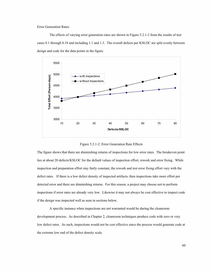
Error Generation Rates

The effects of varying error generation rates are shown in Figure 5.2.1-2 from the results of test

cases 8.1 through 8.18 and including 1.1 and 1.3. The overall defects per KSLOC are split evenly between

design and code for the data points in the figure.

3000

3500

4000

4500

5000

5500

10 20 30 40 50 60 70 80

Defects/KSLOC

Tota

l Effo

rt (P

erso

n-da

ys) w ith inspections

w ithout inspections

Figure 5.2.1-2: Error Generation Rate Effects

The figure shows that there are diminishing returns of inspections for low error rates. The breakeven point

lies at about 20 defects/KSLOC for the default values of inspection effort, rework and error fixing. While

inspection and preparation effort stay fairly constant, the rework and test error fixing effort vary with the

defect rates. If there is a low defect density of inspected artifacts, then inspections take more effort per

detected error and there are diminishing returns. For this reason, a project may choose not to perform

inspections if error rates are already very low. Likewise it may not always be cost effective to inspect code

if the design was inspected well as seen in sections below.

A specific instance when inspections are not warranted would be during the cleanroom

development process. As described in Chapter 2, cleanroom techniques produce code with zero or very

low defect rates. As such, inspections would not be cost effective since the process would generate code at

the extreme low end of the defect density scale.

60

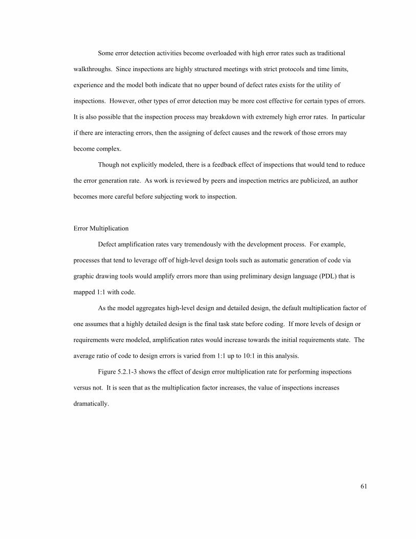
Some error detection activities become overloaded with high error rates such as traditional

walkthroughs. Since inspections are highly structured meetings with strict protocols and time limits,

experience and the model both indicate that no upper bound of defect rates exists for the utility of

inspections. However, other types of error detection may be more cost effective for certain types of errors.

It is also possible that the inspection process may breakdown with extremely high error rates. In particular

if there are interacting errors, then the assigning of defect causes and the rework of those errors may

become complex.

Though not explicitly modeled, there is a feedback effect of inspections that would tend to reduce

the error generation rate. As work is reviewed by peers and inspection metrics are publicized, an author

becomes more careful before subjecting work to inspection.

Error Multiplication

Defect amplification rates vary tremendously with the development process. For example,

processes that tend to leverage off of high-level design tools such as automatic generation of code via

graphic drawing tools would amplify errors more than using preliminary design language (PDL) that is

mapped 1:1 with code.

As the model aggregates high-level design and detailed design, the default multiplication factor of

one assumes that a highly detailed design is the final task state before coding. If more levels of design or

requirements were modeled, amplification rates would increase towards the initial requirements state. The

average ratio of code to design errors is varied from 1:1 up to 10:1 in this analysis.

Figure 5.2.1-3 shows the effect of design error multiplication rate for performing inspections

versus not. It is seen that as the multiplication factor increases, the value of inspections increases

dramatically.

61

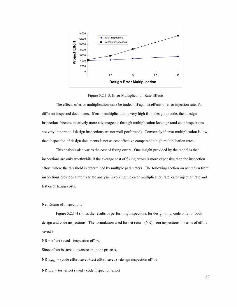
0

2000

4000

6000

8000

10000

12000

14000

1 2.5 5 7.5

Design Error Multiplication

Proj

ect E

ffort

10

w ith inspections

w ithout inspections

Figure 5.2.1-3: Error Multiplication Rate Effects

The effects of error multiplication must be traded off against effects of error injection rates for

different inspected documents. If error multiplication is very high from design to code, then design

inspections become relatively more advantageous through multiplication leverage (and code inspections

are very important if design inspections are not well-performed). Conversely if error multiplication is low,

then inspection of design documents is not as cost effective compared to high multiplication rates.

This analysis also varies the cost of fixing errors. One insight provided by the model is that

inspections are only worthwhile if the average cost of fixing errors is more expensive than the inspection

effort, where the threshold is determined by multiple parameters. The following section on net return from

inspections provides a multivariate analysis involving the error multiplication rate, error injection rate and

test error fixing costs.

Net Return of Inspections

Figure 5.2.1-4 shows the results of performing inspections for design only, code only, or both

design and code inspections. The formulation used for net return (NR) from inspections in terms of effort

saved is

NR = effort saved - inspection effort.

Since effort is saved downstream in the process,

NR design = (code effort saved+test effort saved) - design inspection effort

NR code = test effort saved - code inspection effort

62

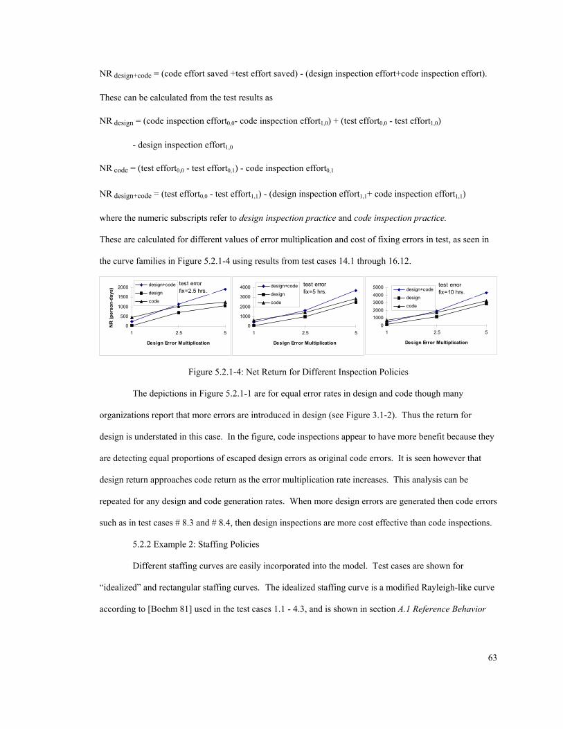
NR design+code = (code effort saved +test effort saved) - (design inspection effort+code inspection effort).

These can be calculated from the test results as

NR design = (code inspection effort0,0- code inspection effort1,0) + (test effort0,0 - test effort1,0)

- design inspection effort1,0

NR code = (test effort0,0 - test effort0,1) - code inspection effort0,1

NR design+code = (test effort0,0 - test effort1,1) - (design inspection effort1,1+ code inspection effort1,1)

where the numeric subscripts refer to design inspection practice and code inspection practice.

These are calculated for different values of error multiplication and cost of fixing errors in test, as seen in

the curve families in Figure 5.2.1-4 using results from test cases 14.1 through 16.12.

0

500

1000

1500

2000

1 2.5 5

Design Error Multiplication

NR

(per

son-

days

) design+code

design

code

test error fix=2.5 hrs.

0

1000

2000

3000

4000

1 2.5 5

Design Error Multiplication

design+code

design

code

test error fix=5 hrs.

010002000300040005000

1 2.5

Design Error Multiplication

5

design+code

design

code

test error fix=10 hrs.

Figure 5.2.1-4: Net Return for Different Inspection Policies

The depictions in Figure 5.2.1-1 are for equal error rates in design and code though many

organizations report that more errors are introduced in design (see Figure 3.1-2). Thus the return for

design is understated in this case. In the figure, code inspections appear to have more benefit because they

are detecting equal proportions of escaped design errors as original code errors. It is seen however that

design return approaches code return as the error multiplication rate increases. This analysis can be

repeated for any design and code generation rates. When more design errors are generated then code errors

such as in test cases # 8.3 and # 8.4, then design inspections are more cost effective than code inspections.

5.2.2 Example 2: Staffing Policies

Different staffing curves are easily incorporated into the model. Test cases are shown for

“idealized” and rectangular staffing curves. The idealized staffing curve is a modified Rayleigh-like curve

according to [Boehm 81] used in the test cases 1.1 - 4.3, and is shown in section A.1 Reference Behavior

63

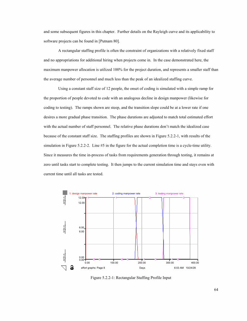
and some subsequent figures in this chapter. Further details on the Rayleigh curve and its applicability to

software projects can be found in [Putnam 80].

A rectangular staffing profile is often the constraint of organizations with a relatively fixed staff

and no appropriations for additional hiring when projects come in. In the case demonstrated here, the

maximum manpower allocation is utilized 100% for the project duration, and represents a smaller staff than

the average number of personnel and much less than the peak of an idealized staffing curve.

Using a constant staff size of 12 people, the onset of coding is simulated with a simple ramp for

the proportion of people devoted to code with an analogous decline in design manpower (likewise for

coding to testing). The ramps shown are steep, and the transition slope could be at a lower rate if one

desires a more gradual phase transition. The phase durations are adjusted to match total estimated effort

with the actual number of staff personnel. The relative phase durations don’t match the idealized case

because of the constant staff size. The staffing profiles are shown in Figure 5.2.2-1, with results of the

simulation in Figure 5.2.2-2. Line #5 in the figure for the actual completion time is a cycle-time utility.

Since it measures the time in-process of tasks from requirements generation through testing, it remains at

zero until tasks start to complete testing. It then jumps to the current simulation time and stays even with

current time until all tasks are tested.

6:03 AM 10/24/28

0.00 100.00 200.00 300.00 400.00

Days

1:

1:

1:

2:

2:

2:

3:

3:

3:

0.00

6.00

12.00

0.00

6.00

12.00

2: coding manpower rate 3: testing manpower rate

1 1

1 12 2

2

23 3 3

3

effort graphs: Page 8

1: design manpower rate

Figure 5.2.2-1: Rectangular Staffing Profile Input

64

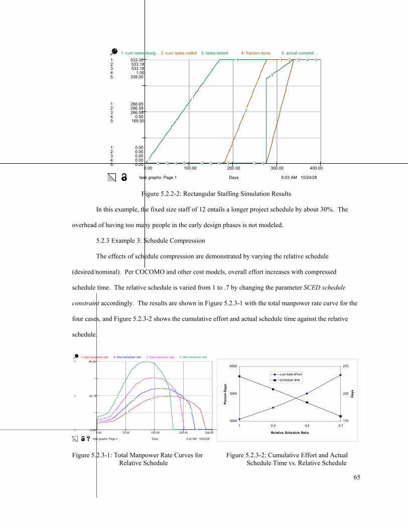
6:03 AM 10/24/28

0.00 100.00 200.00 300.00 400.00

Days

1:

1:

1:

2:

2:

2:

3:

3:

3:

4:

4:

4:

5:

5:

5:

0.00

266.65

533.30

0.00

266.59

533.18

0.00

266.59

533.18

0.00

0.50

1.00

0.00

169.50

339.00

1: cum tasks desig… 3: tasks tested 5: actual completi…

1

1

1 1

2 2

2

2

3 3 3

3

4 4 4

4

5 5

5

5

task graphs: Page 1

2: cum tasks coded 4: fraction done

Figure 5.2.2-2: Rectangular Staffing Simulation Results

In this example, the fixed size staff of 12 entails a longer project schedule by about 30%. The

overhead of having too many people in the early design phases is not modeled.

5.2.3 Example 3: Schedule Compression The effects of schedule compression are demonstrated by varying the relative schedule

(desired/nominal). Per COCOMO and other cost models, overall effort increases with compressed

schedule time. The relative schedule is varied from 1 to .7 by changing the parameter SCED schedule

constraint accordingly. The results are shown in Figure 5.2.3-1 with the total manpower rate curve for the

four cases, and Figure 5.2.3-2 shows the cumulative effort and actual schedule time against the relative

schedule.

4000

5000

6000

1 0.9 0.8 0.7

Relative Schedule Ratio

Pers

on-D

ays

170

220

270

Day

s

cum total effort

schedule time

4:42 AM 10/22/28

0.00 75.00 150.00 225.00 300.00

Days

1:

1:

1:

0.00

24.13

48.25

2: total manpower rate 3: total manpower rate 4: total manpower rate1: total manpower rate

1

1

11

2

2

2

2

3

3 3

3

4

4

4 4

task graphs: Page 4

Figure 5.2.3-1: Total Manpower Rate Curves for Figure 5.2.3-2: Cumulative Effort and Actual Relative Schedule Schedule Time vs. Relative Schedule

65

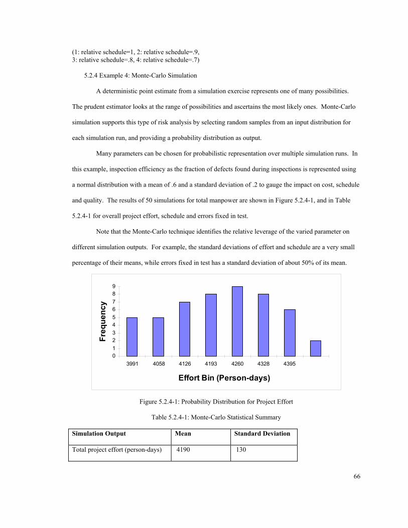
(1: relative schedule=1, 2: relative schedule=.9, 3: relative schedule=.8, 4: relative schedule=.7)

5.2.4 Example 4: Monte-Carlo Simulation

A deterministic point estimate from a simulation exercise represents one of many possibilities.

The prudent estimator looks at the range of possibilities and ascertains the most likely ones. Monte-Carlo

simulation supports this type of risk analysis by selecting random samples from an input distribution for

each simulation run, and providing a probability distribution as output.

Many parameters can be chosen for probabilistic representation over multiple simulation runs. In

this example, inspection efficiency as the fraction of defects found during inspections is represented using

a normal distribution with a mean of .6 and a standard deviation of .2 to gauge the impact on cost, schedule

and quality. The results of 50 simulations for total manpower are shown in Figure 5.2.4-1, and in Table

5.2.4-1 for overall project effort, schedule and errors fixed in test.

Note that the Monte-Carlo technique identifies the relative leverage of the varied parameter on

different simulation outputs. For example, the standard deviations of effort and schedule are a very small

percentage of their means, while errors fixed in test has a standard deviation of about 50% of its mean.

0123456789

3991 4058 4126 4193 4260 4328 4395

Effort Bin (Person-days)

Freq

uenc

y

Figure 5.2.4-1: Probability Distribution for Project Effort

Table 5.2.4-1: Monte-Carlo Statistical Summary

Simulation Output Mean Standard Deviation

Total project effort (person-days) 4190 130

66

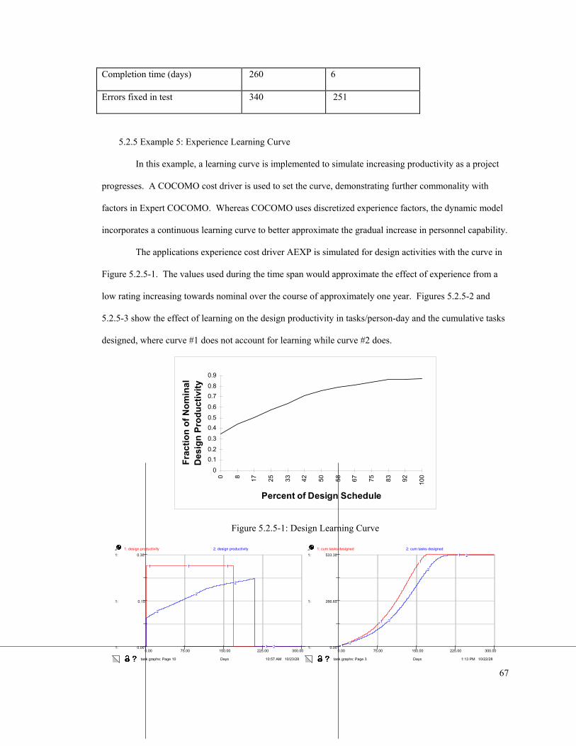
Completion time (days) 260 6

Errors fixed in test 340 251

5.2.5 Example 5: Experience Learning Curve

In this example, a learning curve is implemented to simulate increasing productivity as a project

progresses. A COCOMO cost driver is used to set the curve, demonstrating further commonality with

factors in Expert COCOMO. Whereas COCOMO uses discretized experience factors, the dynamic model

incorporates a continuous learning curve to better approximate the gradual increase in personnel capability.

The applications experience cost driver AEXP is simulated for design activities with the curve in

Figure 5.2.5-1. The values used during the time span would approximate the effect of experience from a

low rating increasing towards nominal over the course of approximately one year. Figures 5.2.5-2 and

5.2.5-3 show the effect of learning on the design productivity in tasks/person-day and the cumulative tasks

designed, where curve #1 does not account for learning while curve #2 does.

0

0.10.2

0.3

0.40.5

0.6

0.70.8

0.9

0 8 17 25 33 42 50 58 67 75 83 92 100

Percent of Design Schedule

Frac

tion

of N

omin

al

Des

ign

Prod

uctiv

ity

Figure 5.2.5-1: Design Learning Curve

1:13 PM 10/22/28

0.00 75.00 150.00 225.00 300.00

Days

1:

1:

1:

0.00

266.65

533.30

2: cum tasks designed

1

1

1

1

2

2

2

2

task graphs: Page 3 10:57 AM 10/23/28

0.00 75.00 150.00 225.00 300.00

Days

1:

1:

1:

0.00

0.15

0.30

2: design productivity1: design productivity 1: cum tasks designed

1 1 1

1

2

2

2

2

task graphs: Page 10

67

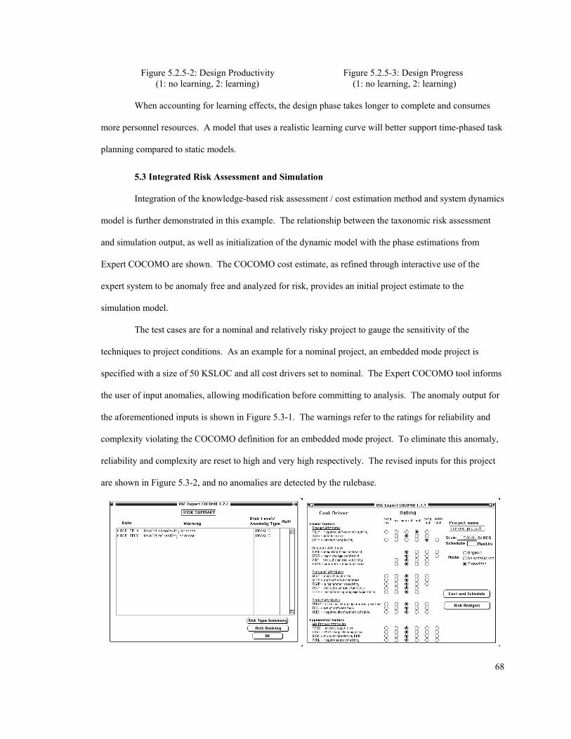
Figure 5.2.5-2: Design Productivity Figure 5.2.5-3: Design Progress (1: no learning, 2: learning) (1: no learning, 2: learning) When accounting for learning effects, the design phase takes longer to complete and consumes

more personnel resources. A model that uses a realistic learning curve will better support time-phased task

planning compared to static models.

5.3 Integrated Risk Assessment and Simulation

Integration of the knowledge-based risk assessment / cost estimation method and system dynamics

model is further demonstrated in this example. The relationship between the taxonomic risk assessment

and simulation output, as well as initialization of the dynamic model with the phase estimations from

Expert COCOMO are shown. The COCOMO cost estimate, as refined through interactive use of the

expert system to be anomaly free and analyzed for risk, provides an initial project estimate to the

simulation model.

The test cases are for a nominal and relatively risky project to gauge the sensitivity of the

techniques to project conditions. As an example for a nominal project, an embedded mode project is

specified with a size of 50 KSLOC and all cost drivers set to nominal. The Expert COCOMO tool informs

the user of input anomalies, allowing modification before committing to analysis. The anomaly output for

the aforementioned inputs is shown in Figure 5.3-1. The warnings refer to the ratings for reliability and

complexity violating the COCOMO definition for an embedded mode project. To eliminate this anomaly,

reliability and complexity are reset to high and very high respectively. The revised inputs for this project

are shown in Figure 5.3-2, and no anomalies are detected by the rulebase.

68

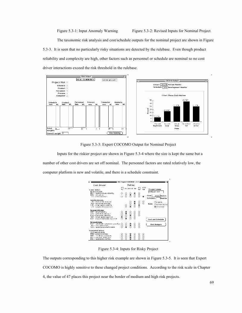
Figure 5.3-1: Input Anomaly Warning Figure 5.3-2: Revised Inputs for Nominal Project

The taxonomic risk analysis and cost/schedule outputs for the nominal project are shown in Figure

5.3-3. It is seen that no particularly risky situations are detected by the rulebase. Even though product

reliability and complexity are high, other factors such as personnel or schedule are nominal so no cost

driver interactions exceed the risk threshold in the rulebase.

Figure 5.3-3: Expert COCOMO Output for Nominal Project

Inputs for the riskier project are shown in Figure 5.3-4 where the size is kept the same but a

number of other cost drivers are set off nominal. The personnel factors are rated relatively low, the

computer platform is new and volatile, and there is a schedule constraint.

Figure 5.3-4: Inputs for Risky Project

The outputs corresponding to this higher risk example are shown in Figure 5.3-5. It is seen that Expert

COCOMO is highly sensitive to these changed project conditions. According to the risk scale in Chapter

4, the value of 47 places this project near the border of medium and high risk projects. 69

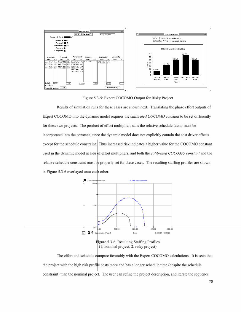
Figure 5.3-5: Expert COCOMO Output for Risky Project

Results of simulation runs for these cases are shown next. Translating the phase effort outputs of

Expert COCOMO into the dynamic model requires the calibrated COCOMO constant to be set differently

for these two projects. The product of effort multipliers sans the relative schedule factor must be

incorporated into the constant, since the dynamic model does not explicitly contain the cost driver effects

except for the schedule constraint. Thus increased risk indicates a higher value for the COCOMO constant

used in the dynamic model in lieu of effort multipliers, and both the calibrated COCOMO constant and the

relative schedule constraint must be properly set for these cases. The resulting staffing profiles are shown

in Figure 5.3-6 overlayed onto each other.

8:59 AM 10/22/28

0.00 175.00 350.00 525.00 700.00

Days

1:

1:

1:

0.00

45.39

90.77

1: total manpower rate 2: total manpower rate

1

1

1 1

2

2

2

task graphs: Page 7

Figure 5.3-6: Resulting Staffing Profiles (1: nominal project, 2: risky project)

The effort and schedule compare favorably with the Expert COCOMO calculations. It is seen that

the project with the high risk profile costs more and has a longer schedule time (despite the schedule

constraint) than the nominal project. The user can refine the project description, and iterate the sequence

70

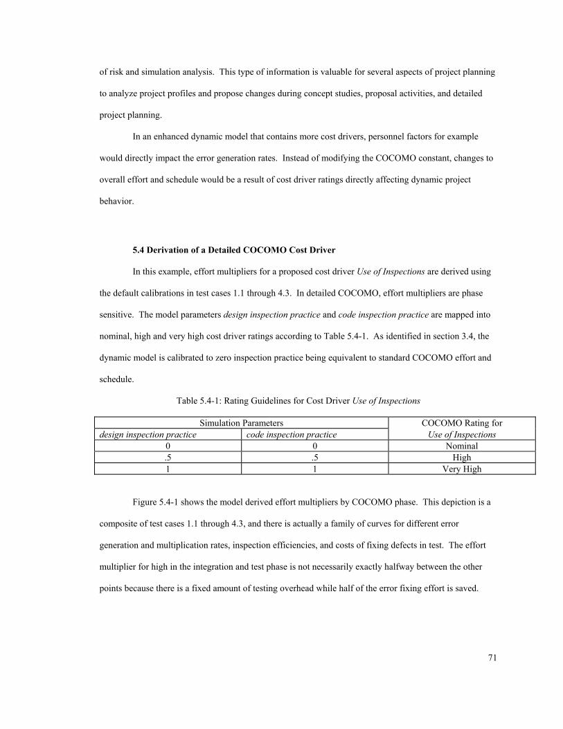
of risk and simulation analysis. This type of information is valuable for several aspects of project planning

to analyze project profiles and propose changes during concept studies, proposal activities, and detailed

project planning.

In an enhanced dynamic model that contains more cost drivers, personnel factors for example

would directly impact the error generation rates. Instead of modifying the COCOMO constant, changes to

overall effort and schedule would be a result of cost driver ratings directly affecting dynamic project

behavior.

5.4 Derivation of a Detailed COCOMO Cost Driver

In this example, effort multipliers for a proposed cost driver Use of Inspections are derived using

the default calibrations in test cases 1.1 through 4.3. In detailed COCOMO, effort multipliers are phase

sensitive. The model parameters design inspection practice and code inspection practice are mapped into

nominal, high and very high cost driver ratings according to Table 5.4-1. As identified in section 3.4, the

dynamic model is calibrated to zero inspection practice being equivalent to standard COCOMO effort and

schedule.

Table 5.4-1: Rating Guidelines for Cost Driver Use of Inspections

Simulation Parameters COCOMO Rating for design inspection practice code inspection practice Use of Inspections

0 0 Nominal .5 .5 High 1 1 Very High

Figure 5.4-1 shows the model derived effort multipliers by COCOMO phase. This depiction is a

composite of test cases 1.1 through 4.3, and there is actually a family of curves for different error

generation and multiplication rates, inspection efficiencies, and costs of fixing defects in test. The effort

multiplier for high in the integration and test phase is not necessarily exactly halfway between the other

points because there is a fixed amount of testing overhead while half of the error fixing effort is saved.

71

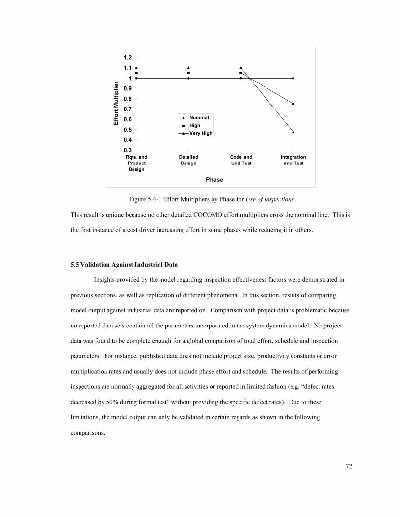
0.3

0.4

0.5

0.6

0.7

0.8

0.9

1

1.1

1.2

Rqts. andProductDesign

DetailedDesign

Code andUnit Test

Integrationand Test

Phase

Effo

rt M

ultip

lier

NominalHighVery High

Figure 5.4-1 Effort Multipliers by Phase for Use of Inspections

This result is unique because no other detailed COCOMO effort multipliers cross the nominal line. This is

the first instance of a cost driver increasing effort in some phases while reducing it in others.

5.5 Validation Against Industrial Data Insights provided by the model regarding inspection effectiveness factors were demonstrated in

previous sections, as well as replication of different phenomena. In this section, results of comparing

model output against industrial data are reported on. Comparison with project data is problematic because

no reported data sets contain all the parameters incorporated in the system dynamics model. No project

data was found to be complete enough for a global comparison of total effort, schedule and inspection

parameters. For instance, published data does not include project size, productivity constants or error

multiplication rates and usually does not include phase effort and schedule. The results of performing

inspections are normally aggregated for all activities or reported in limited fashion (e.g. “defect rates

decreased by 50% during formal test” without providing the specific defect rates). Due to these

limitations, the model output can only be validated in certain regards as shown in the following

comparisons.

72

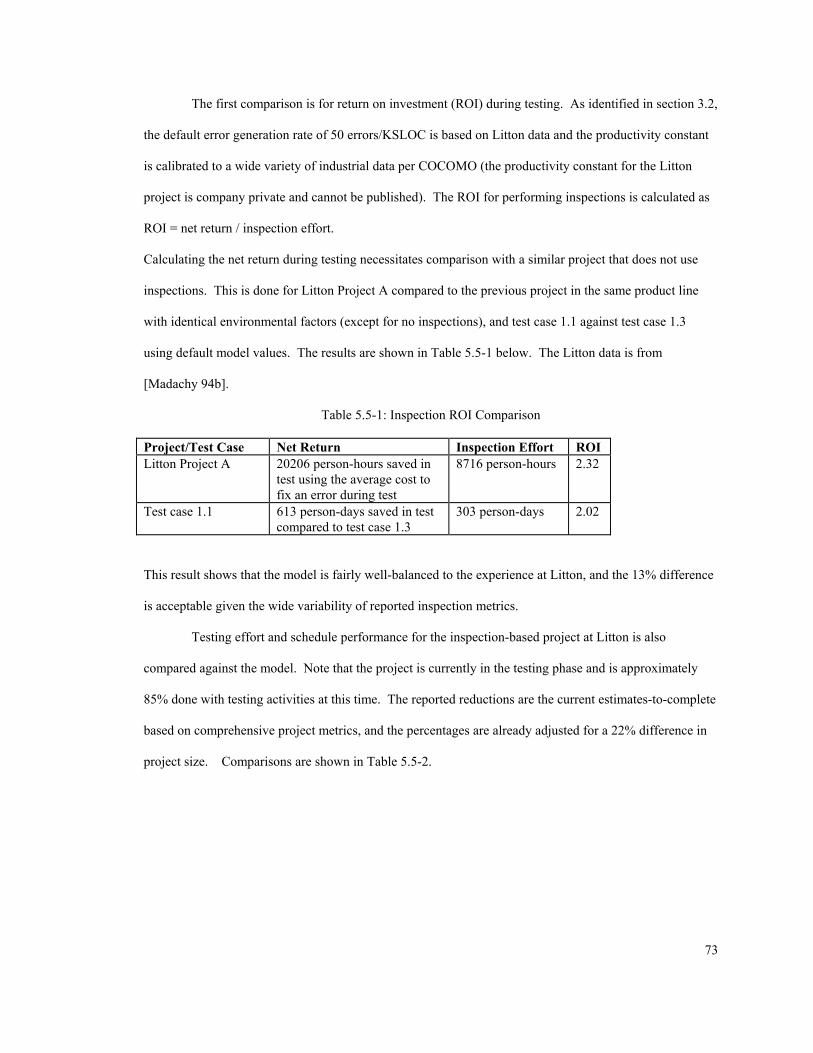
The first comparison is for return on investment (ROI) during testing. As identified in section 3.2,

the default error generation rate of 50 errors/KSLOC is based on Litton data and the productivity constant

is calibrated to a wide variety of industrial data per COCOMO (the productivity constant for the Litton

project is company private and cannot be published). The ROI for performing inspections is calculated as

ROI = net return / inspection effort.

Calculating the net return during testing necessitates comparison with a similar project that does not use

inspections. This is done for Litton Project A compared to the previous project in the same product line

with identical environmental factors (except for no inspections), and test case 1.1 against test case 1.3

using default model values. The results are shown in Table 5.5-1 below. The Litton data is from

[Madachy 94b].

Table 5.5-1: Inspection ROI Comparison

Project/Test Case Net Return Inspection Effort ROI Litton Project A 20206 person-hours saved in

test using the average cost to fix an error during test

8716 person-hours 2.32

Test case 1.1 613 person-days saved in test compared to test case 1.3

303 person-days 2.02

This result shows that the model is fairly well-balanced to the experience at Litton, and the 13% difference

is acceptable given the wide variability of reported inspection metrics.

Testing effort and schedule performance for the inspection-based project at Litton is also

compared against the model. Note that the project is currently in the testing phase and is approximately

85% done with testing activities at this time. The reported reductions are the current estimates-to-complete

based on comprehensive project metrics, and the percentages are already adjusted for a 22% difference in

project size. Comparisons are shown in Table 5.5-2.

73

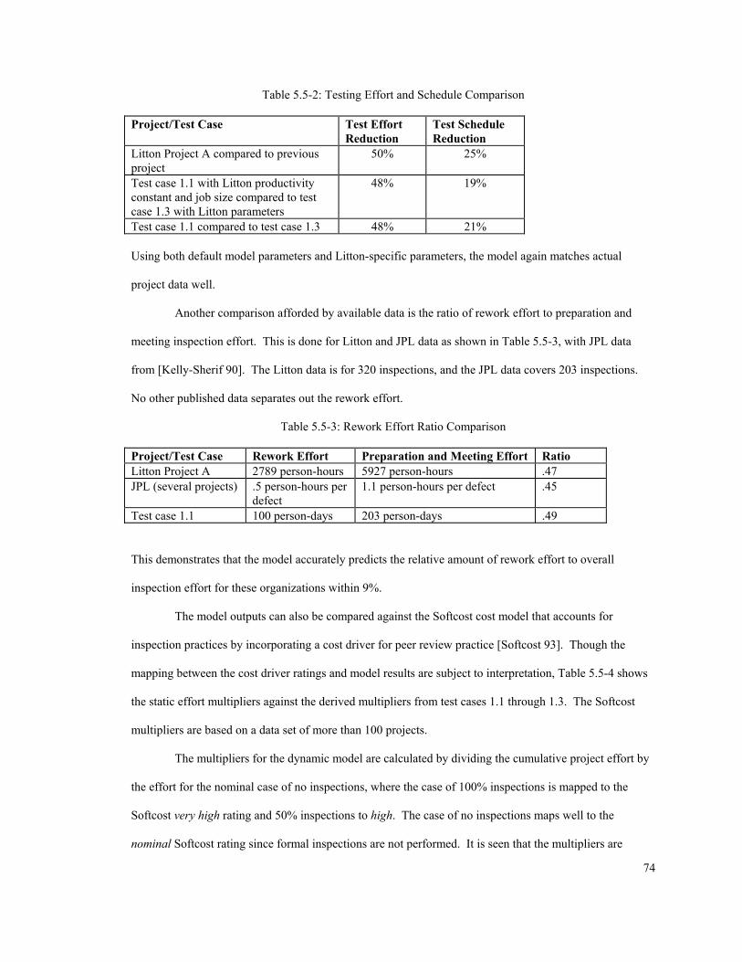
Table 5.5-2: Testing Effort and Schedule Comparison

Project/Test Case Test Effort Reduction

Test Schedule Reduction

Litton Project A compared to previous project

50% 25%

Test case 1.1 with Litton productivity constant and job size compared to test case 1.3 with Litton parameters

48% 19%

Test case 1.1 compared to test case 1.3 48% 21% Using both default model parameters and Litton-specific parameters, the model again matches actual

project data well.

Another comparison afforded by available data is the ratio of rework effort to preparation and

meeting inspection effort. This is done for Litton and JPL data as shown in Table 5.5-3, with JPL data

from [Kelly-Sherif 90]. The Litton data is for 320 inspections, and the JPL data covers 203 inspections.

No other published data separates out the rework effort.

Table 5.5-3: Rework Effort Ratio Comparison

Project/Test Case Rework Effort Preparation and Meeting Effort Ratio Litton Project A 2789 person-hours 5927 person-hours .47 JPL (several projects) .5 person-hours per

defect 1.1 person-hours per defect .45

Test case 1.1 100 person-days 203 person-days .49

This demonstrates that the model accurately predicts the relative amount of rework effort to overall

inspection effort for these organizations within 9%.

The model outputs can also be compared against the Softcost cost model that accounts for

inspection practices by incorporating a cost driver for peer review practice [Softcost 93]. Though the

mapping between the cost driver ratings and model results are subject to interpretation, Table 5.5-4 shows

the static effort multipliers against the derived multipliers from test cases 1.1 through 1.3. The Softcost

multipliers are based on a data set of more than 100 projects.

The multipliers for the dynamic model are calculated by dividing the cumulative project effort by

the effort for the nominal case of no inspections, where the case of 100% inspections is mapped to the

Softcost very high rating and 50% inspections to high. The case of no inspections maps well to the

nominal Softcost rating since formal inspections are not performed. It is seen that the multipliers are

74

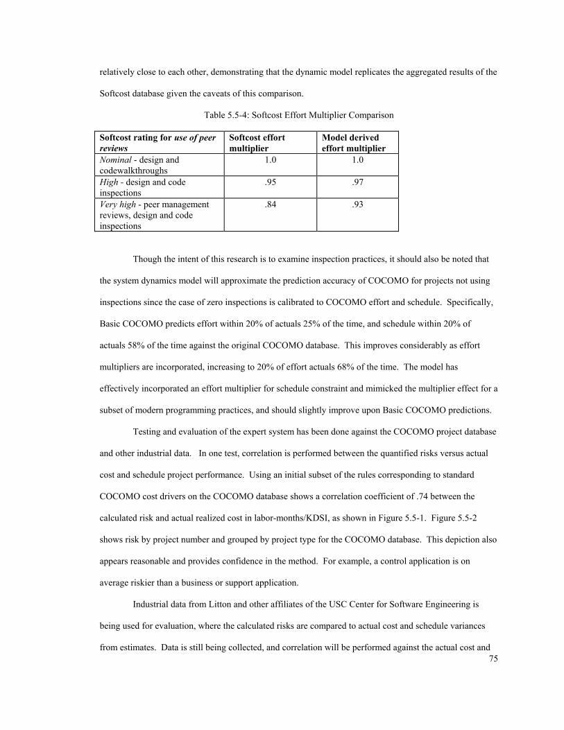
relatively close to each other, demonstrating that the dynamic model replicates the aggregated results of the

Softcost database given the caveats of this comparison.

Table 5.5-4: Softcost Effort Multiplier Comparison

Softcost rating for use of peer reviews

Softcost effort multiplier

Model derived effort multiplier

Nominal - design and codewalkthroughs

1.0 1.0

High - design and code inspections

.95 .97

Very high - peer management reviews, design and code inspections

.84 .93

Though the intent of this research is to examine inspection practices, it should also be noted that

the system dynamics model will approximate the prediction accuracy of COCOMO for projects not using

inspections since the case of zero inspections is calibrated to COCOMO effort and schedule. Specifically,

Basic COCOMO predicts effort within 20% of actuals 25% of the time, and schedule within 20% of

actuals 58% of the time against the original COCOMO database. This improves considerably as effort

multipliers are incorporated, increasing to 20% of effort actuals 68% of the time. The model has

effectively incorporated an effort multiplier for schedule constraint and mimicked the multiplier effect for a

subset of modern programming practices, and should slightly improve upon Basic COCOMO predictions.

Testing and evaluation of the expert system has been done against the COCOMO project database

and other industrial data. In one test, correlation is performed between the quantified risks versus actual

cost and schedule project performance. Using an initial subset of the rules corresponding to standard

COCOMO cost drivers on the COCOMO database shows a correlation coefficient of .74 between the

calculated risk and actual realized cost in labor-months/KDSI, as shown in Figure 5.5-1. Figure 5.5-2

shows risk by project number and grouped by project type for the COCOMO database. This depiction also

appears reasonable and provides confidence in the method. For example, a control application is on

average riskier than a business or support application.

75

Industrial data from Litton and other affiliates of the USC Center for Software Engineering is

being used for evaluation, where the calculated risks are compared to actual cost and schedule variances

from estimates. Data is still being collected, and correlation will be performed against the actual cost and

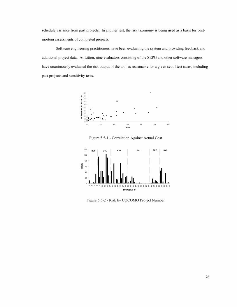
schedule variance from past projects. In another test, the risk taxonomy is being used as a basis for post-

mortem assessments of completed projects.

Software engineering practitioners have been evaluating the system and providing feedback and

additional project data. At Litton, nine evaluators consisting of the SEPG and other software managers

have unanimously evaluated the risk output of the tool as reasonable for a given set of test cases, including

past projects and sensitivity tests.

RISK

PER

SON

-MO

NTH

S / K

DSI

0

5

10

15

20

25

30

35

40

45

50

0 20 40 60 80 100 120

Figure 5.5-1 - Correlation Against Actual Cost

PROJECT #

RIS

K

0

20

40

60

80

100

120

1 3 5 7 9 11 13 15 17 19 21 23 25 27 29 31 33 35 37 39 41 43 45 47 49 51 53 55 57 59 61 63

HMI SCIBUS CTL SUP SYS

Figure 5.5-2 - Risk by COCOMO Project Number

76

5.6 Evaluation Summary

A detailed validation summary is provided in Appendix A. All variables in the reference behavior

in section A.1 seem reasonable. For each validation test in section A.3 based on the criteria in Table 5-1,

an assessment is made as to how well the model performed, and plans are provided for future enhancement

where applicable. No outright failures are identified. Experts that were interviewed have also evaluated

the reasonableness of the time history output, the quantitative effects of inspections, and found no major

deficiencies.

The model is shown to be suitable for its expressed purpose of demonstrating the effects of

inspections from both structural and behavioral perspectives. Policy conclusions are sensitive to

reasonable parameter variations of error generation and inspection efficiency. The model is also shown to

be consistent with reality by comparison with project data, idealized inspection trends and expert

experience. It is useful and effective as a suitable model because it is appropriate for an audience of

software practitioners and provides new insights into the development process.

The model has met its goals of demonstrating the behavior of a project using an inspection-based

process and is able to predict the relative change in effort, schedule and quality using inspections. When

properly calibrated for specific environments, the model is expected to show high fidelity. The results of

the experiments support the original hypothesis that a system dynamics model can be developed of various

aspects of an inspection-based process.

77

Chapter 6 Conclusions

This chapter provides a summary of research results. After a summary of previous chapters in

Section 6.1, specific research contributions are presented in Section 6.2. Following that, directions for

future research are provided in Section 6.3.

6.1 Research Summary

In Chapter 1, an introduction to the research problem was presented. There is a knowledge gap

for interdependent software project phenomena. Without models that integrate various aspects of the

software process, practitioners will continue to encounter problems in project planning, development, and

process improvement.

Chapter 2 provided a comprehensive background of literature and research in the relevant areas of

software engineering, simulation and software project dynamics. The areas of process technology, cost

estimation, risk management and knowledge-based software engineering have much to bear on each other.

A challenge of research is to integrate the various perspectives and techniques for the purposes of project

management and process improvement.

Chapters 3 and 4 highlighted original modeling done for an inspection-based process and

taxonomic risk assessment. Inspections are a method to reduce software defects, and the model was

developed to investigate the incorporation of inspections in the development process. The knowledge-

based risk assessment scheme was developed to support risk management, and leverages on information

from cost estimation.

Chapter 5 showed that the system dynamics model has successfully demonstrated several

phenomena of software projects, including the effects of inspections and management decision policies. It

was also shown that the model is scalable for project size and calibratable for productivity, error generation

and error detection.

78

The model demonstrates that performing inspections slightly increases development effort and

decreases effort and schedule in testing and integration, with the effect relatively linear as more inspections

are performed. It shows that the cost effectiveness of inspections depends on phase error injection rates,

error amplification, testing error fixing effort and inspection efficiency.

The user can specify nominal error rates as well as the efficiencies of error detection during

inspection. With increased errors, the model demonstrates that more effort is required in rework and

testing activities to fix the errors. Increased inspection efficiency results in increased rework effort from

inspections and less effort in testing and integration.

The model accounts for the effects of relative schedule (desired/nominal) which is related to the

COCOMO cost driver SCED. With a reduced schedule, the average personnel level increases and the

overall cost goes up. Different staffing curves can also be easily incorporated into the model. Test cases

are shown for rectangular and idealized staffing curves with corresponding project results.

Complementary features of dynamic and static models for the software process were also shown.

Intersection of the dynamic model with the static COCOMO was demonstrated in several regards. Phase

effort and schedule from COCOMO was used to nominally calibrate the dynamic model, and the dynamic

model furthers COCOMO by accounting for dynamic error generation. Common factors for schedule

constraint and experience factors were used, with the dynamic model improving on static assumptions.

Integration of Expert COCOMO and the dynamic model was also demonstrated, as well as derivation of a

COCOMO cost driver from the simulation results.

6.2 Contributions

This research has demonstrated the dynamic effects of performing inspections and contributed to

the body of knowledge regarding the interrelated factors of inspection effectiveness. The model

successfully demonstrates the behavior of a project using an inspection-based process and is able to predict

the relative change in effort, schedule and quality when using inspections. It will support ongoing research

since updated model parameters can be easily incorporated. This work has also corroborated that system

dynamics is a suitable modeling paradigm for software processes in general and shown that such modeling

can be augmented with expert heuristics to support process management. The combined dynamic model

and knowledge-based project assessment also supports risk management in several regards.

This research has also examined complementary features of dynamic and static models of the

software development process. It was shown how a static model can be used to nominally calibrate a

79

dynamic model, and the dynamic model then incorporating more realistic assumptions of time-varying

phenomena. The dynamic model was also used to derive effort multipliers for a static model.

This is a step towards developing a unified model incorporating additional lifecycle process

variations. Such a model would support behavioral understanding, prediction and evaluation of process

improvement, project planning and system acquisition across a range of alternative processes. Some of the

modeling constructs can be used for other lifecycle process models, such as an evolutionary risk-driven

process since inspections are akin to inserting risk management activities into the lifecycle.

Several facets of this research have been published and presented at conferences or are

forthcoming: [Madachy 94] presented the knowledge-based method for risk assessment and cost

estimation, [Madachy 94a] documents the knowledge-based method being adopted in industrial practice,

[Madachy et al. 93a] discusses analysis of inspection data which supported inspection model parameter

development, and [Madachy 94b] enhances the previous analysis of inspection data and elevates it to an

organizational level. Other aspects of this research, particularly the inspection-based process model, are

being readied for submission to an appropriate refereed journal.

6.3 Directions for Future Research

There are many interesting problems and challenging opportunities for extensions of this research.

An outline of directions for future research are provided in the paragraphs below.

Different error models can be incorporated into the model. There are a variety of alternative

formulations to account for error generation and detection, including multiplication of errors through the

phases. Additionally, accounting for the severity and type of errors would enhance the model and further

support defect prevention and causal analysis efforts. The effects of extremely high error rates should also

be investigated, as the model currently shows no degradation of the inspection process under such

conditions.

The current model does not account for other defect finding activities such as walkthroughs,

cleanroom reviews, etc. Though many organization opt for only inspections, there are various other peer

reviews and new methods of development that warrant examination in a dynamic model.

80

As previously identified, this model examines software production, testing and personnel policies

independent of other factors included in Abdel-Hamid’s model. This model can be integrated with his

model by replacing some portions and adding to others. In particular, the software production sector

would be augmented. Bellcore has translated Abdel-Hamid’s model into ITHINK [Glickman 94] which

could provide a foundation for modification.

The system dynamics model can be enhanced for usability by adding “authoring” capabilities. To

support policy analysis and experimentation, user friendly slide controls for varying model parameters can

be employed with additional software.

An experiment is proposed to compare the discrete-event STATEMATE approach being

developed at the SEI with system dynamics modeling. Raffo is using Kellner's modeling technique to

evaluate the effects of inspections on the process [Raffo 93]. Both approaches can model the effect of

inspections using a common test case, and the discrete and continuous staffing outputs and quality profiles

will be compared. This experiment will help identify the relative merits of both approaches for the

research community.

Numerous variations on the staffing and scheduling policies can be tested. Some implicit policy

assumptions were used in this model regarding the personnel availability and error rates in the delivered

product. Many other possibilities exist besides those investigated here, such as organizations choosing to

deliver a product before all known errors are eliminated. Another possibility is modeling Brooks’ Law

with mentoring costs, assimilation time, and disaggregation of personnel into experience levels.

The system dynamics model can be refined for finer granularity in the phases. Initially, high level

and detailed design can be separated out and requirements activities can eventually be incorporated. Data

exists for calibrating the defect rates of requirements artifacts as documented in [Madachy et al. 93a] and

[Madachy 94b]. The testing and integration phase can also be further disaggregated.

The model could be enhanced to “drill down” further into the inspection process for the purpose

of optimization, and look into the dynamics of inspection efficiency, rates, etc. The factors leading to

overall inspection effectiveness include learning and training effects of authors and inspectors, the number

of inspectors, preparation time, inspection time, inspection rate and the type of document inspected.

81

The dynamic model can be enhanced for additional COCOMO cost drivers, and investigation of

their dynamic effects can be undertaken. Conversely, one can also derive effort multipliers per section 5.4

for different COCOMO drivers by constructing unique models for investigation. For instance, the model

can be used as a platform for varying levels of experience to assist in deriving multiplier weights.

More validation against project data is also desired. The model should be re-tested when more

complete project datasets are available. Any cases where the model does not perform well should be

investigated, and a determination made as to why not. This will likely point to aspects of the model that

need improvement.

Other lifecycle process models can be incorporated such as those identified in Section 2.1.1.1

towards a unified system dynamics model for multiple alternative lifecycle processes. Constructs in this

model may be modified for an evolutionary risk-driven process, the cleanroom process, personal software

process and others.

A variety of enhancements and further research can be undertaken for the knowledge-based

aspect. More refined calibrations are still needed for meaningful risk scales. Consistency with other risk

taxonomies and assessment schemes is also desired, such as the SEI risk assessment method [Carr et al. 93]

and the Software Technology Risk Advisor method of calculating the disparities between functional needs

and capabilities [Toth 94].

Additional data from industrial projects can be collected and analyzed, and the risk taxonomy can

serve as a data collection guide. Other features can be incorporated into the tool such as incremental

development support, additional and refined rules, cost risk analysis using Monte Carlo simulation to

assess the effects of uncertainty in the COCOMO inputs, and automatic sensitivity analysis to vary cost

drivers for risk minimization. Additional rules can be identified and incorporated to handle more cost

driver interactions, cost model constraints, incremental development inheritance rules, rating of consistency

violations and advice. Substantial additions are expected for process related factors and advice to control

the risks.

The currently evolving COCOMO 2.0 model has updated cost and scale drivers relative to the

original COCOMO upon which the risk assessment heuristics in Chapter 4 are based. The risk and

82

anomaly rulebases should be updated to correspond with the new set of cost factors and model definitions.

A working hypothesis for COCOMO 2.0 is that risk assessment should be a feature of the cost model

[Boehm et al. 94a]. The risk assessment scheme can also be incorporated into the WinWin spiral model

prototype [Boehm et al. 93] to support COCOMO negotiation parameters.

One drawback of the integrated model is that it isn’t implemented as a single, cohesive tool. The

software packages used for the taxonomic risk assessment and system dynamics model are not amenable to

integration. A challenge is to overcome this current limitation and integrate them into a unified

application.

83

Bibliography

[Abdel-Hamid 89] Abdel-Hamid T, The dynamics of software project staffing: A system dynamics based simulation approach, IEEE Transactions on Software Engineering, February 1989

[Abdel-Hamid 89a] Abdel-Hamid T, Lessons learned from modeling the dynamics of

software development, Communications of the ACM, December 1989 [Abdel-Hamid 90] Abdel-Hamid T, Investigating the cost/schedule trade-off in software

development, IEEE Software, January 1990 [Abdel-Hamid-Madnick 91] Abdel-Hamid T, Madnick S, Software Project Dynamics. Englewood

Cliffs, NJ, Prentice-Hall, 1991 [Abdel-Hamid 93] Abdel-Hamid T, Adapting, correcting, and perfecting software

estimates: a maintenance metaphor, IEEE Computer, March 1993 [Abdel-Hamid 93a] Abdel-Hamid T, Modeling the dynamics of software reuse: an

integrating system dynamics perspective, Presented at the Sixth Annual Workshop on Software Reuse, Owego, NY, November 1993

[Ackerman et al. 84] Ackerman AF, Fowler P, Ebenau R, Software inspections and the

industrial production of software, in "Software Validation, Inspections-Testing-Verification-Alternatives" (H. Hausen, ed.), New York, NY, Elsevier Science Publishers, 1984, pp. 13-40

[Agresti 86] Agresti W (ed.), New Paradigms for Software Development, IEEE

Computer Society, Washington, D.C., 1986 [Balzer et al. 83] Balzer R, Cheatham T, Green C, Software technology in the 1990's:

using a new paradigm, Computer, Nov. 1983, pp. 39-45 [Baumert-McWhinney 92] Baumert J, McWhinney M, Software Measures and the Capability

Maturity Model. CMU/SEI-92-TR-25, Software Engineering Institute, Pittsburgh, PA, 1992

[Biggerstaff 89] Biggerstaff T, Perlis, eds., Software Reusability. Addison-Wesley,

1989 [Boehm 76] Boehm BW, Software engineering, IEEE Transactions on Computers,

vol. C-25, no. 12, December 1976, pp. 1226-1241 [Boehm 81] Boehm BW, Software Engineering Economics. Englewood Cliffs, NJ,

Prentice-Hall, 1981 [Boehm 88] Boehm BW, A spiral model of software development and enhancement,

IEEE Software, May 1988 [Boehm 89] Boehm BW, Software Risk Management. Washington, D. C., IEEE-

CS Press, 1989

84

[Boehm 92] Boehm BW, Knowledge-based process assistance for large software projects, white paper in response to Rome Laboratories PRDS #92-08-PKRD, USC, November, 1992

[Boehm 94] Boehm BW, COCOMO 2.0 program preliminary prospectus.

Proceedings of the USC Center for Software Engineering Annual Research Review, USC, February 1994

[Boehm-Belz 88] Boehm BW, Belz F, Applying process programming to the spiral

model, Proceedings, Fourth International Software Process Workshop, ACM, May 1988

[Boehm-Papaccio 88] Boehm BW, Papaccio PN, Understanding and controlling software

costs, IEEE Transactions on Software Engineering, October 1988 [Boehm-Royce 89] Boehm BW, Royce WE, Ada COCOMO and the Ada process model,

Proceedings, Fifth COCOMO Users' Group Meeting, SEI, October 1989

[Boehm et al. 93] Boehm BW, Bose P, Horowitz E, Scacchi W, and others, Next

generation process models and their environment support, Proceedings of the USC Center for Software Engineering Convocation, USC, June 1993

[Boehm et al. 94] Boehm BW, Horowitz E, Bose P, Balzer R, White paper: draft options

for integrated software product/process technology in satellite ground station and operations control center domains, working paper to be submitted to DARPA, USC, January 1994

[Boehm et al. 94a] Boehm BW, and others, COCOMO 2.0 program preliminary

prospectus, USC Center for Software Engineering, USC, May 1994 [Boehm-Scherlis 92] Boehm BW, Scherlis WL, Megaprogamming, DARPA, 1992 [Brooks 75] Brooks FP, The Mythical Man-Month, Reading, MA, Addison Wesley,

1975 [Buck-Dobbins 84] Buck R, Dobbins J, Application of software inspection methodology in

design and code, in "Software Validation, Inspections-Testing-Verification-Alternatives" (H. Hausen, ed.), New York, NY, Elsevier Science Publishers, 1984, pp. 41-56

[Carr et al. 93] Carr M, Konda S, Monarch I, Ulrich F, Walker C, Taxonomy-Based

Risk Identification, Technical Report CMU/SEI-93-TR-06, Software Engineering Institute, 1993

[Charette 89] Charette RN, Software Engineering Risk Analysis and Management,

McGraw-Hill, 1989 [Cohen 91] Cohen S, Process and products for software reuse and domain

analysis, Software Engineering Institute, Pittsburgh, PA, 1991

85

[Conte et al. 86] Conte S, Dunsmore H, Shen V: Software Engineering Metrics and Models. Menlo Park, CA, Benjamin/Cummings Publishing Co., Inc, 1986

[Curtis et al. 92] Curtis B, Kellner M, Over J, Process modeling, Communications of

the ACM, September 1992 [Danner 91] Danner B, Integrating Reuse into a lifecycle process, STARS '91

Proceedings, STARS Technology Center, Arlington, VA, December 1991

[Davis 88] Davis A, Bersoff E, Comer E, A strategy for comparing alternative

software development life cycle models, IEEE Transactions on Software Engineering, October 1988

[Day 87] Day V, Expert System Cost Model (ESCOMO) Prototype, Proceedings,

Third Annual COCOMO Users' Group Meeting, SEI, November 1987 [Demarco 91] Demarco T, Lister T: Controlling Software Projects: Management,

Measurement and Estimation, The Atlantic Systems Guild, New York, 1991

[Fagan 76] Fagan ME, Design and code inspections to reduce errors in program

development, IBM Systems Journal, V. 15, no. 3, 1976, pp. 182-210 [Fagan 86] Fagan ME, Advances in software inspections, IEEE Transactions on

Software Engineering, V. SE-12, no. 7, July 1986, pp. 744-751 [Feiler-Humphrey 93] Feiler P, Humphrey W, Software process development and enactment:

concepts and definitions. Proceedings of the Second International Conference on the Software Process, IEEE Computer Society, Washington D.C., 1993

[Fenton 91] Fenton N, Software Metrics - A Rigorous Approach, Chapman and

Hall, Great Britain, 1991 [Fishwick-Luker 91] Fishwick P, Luker P (eds.), Qualitative Simulation Modeling and

Analysis, Springer-Verlag, New York, NY, 1991 [Fishwick-Modjeski 91] Fishwick P, Modjeski R (eds.), Knowledge-Based Simulation,

Springer-Verlag, New York, NY, 1991 [Forrester 61] Forrester JW, Industrial Dynamics. Cambridge, MA: MIT Press, 1961 [Forrester 68] Forrester JW, Principles of Systems. Cambridge, MA: MIT Press,

1968 [Forrester -Senge 80] Forrester JW, Senge P, Tests for building confidence in system

dynamics models, in A. Legasto et al. (eds.), TIMS Studies in the Management Sciences (System Dynamics), North-Holland, The Netherlands, 1980, pp. 209-228

86

[Freedman-Weinberg 82] Freedman D, Weinberg G, Handbook of Walkthroughs, Inspections, and Technical Reviews: Evaluating Program, Projects and Products, Little Brown, 1982

[Gilb 88] Gilb T, Principles of Software Engineering Management. Addison-

Wesley, Wokingham, England, 1988 [Glickman 94] Glickman S, The Bellcore-CSELT collaborative project, Proceedings

of the Ninth International Forum on COCOMO and Software Cost Modeling, USC, Los Angeles, CA, 1994

[Goethert et al. 92] Goethert W, Bailey E, Busby M, Software Effort and Schedule

Measurement: A Framework for Counting Staff Hours and Reporting Schedule Information. CMU/SEI-92-TR-21, Software Engineering Institute, Pittsburgh, PA, 1992

[Grady 87] Grady R, Caswell D, Software Metrics: Establishing a Company-Wide

Program. Prentice-Hall, Englewood Cliffs, NJ, 1987 [Grady 92] Grady R, Caswell D, Practical Software Metrics for Project

Management and Process Improvement Prentice-Hall, Englewood Cliffs, NJ, 1992

[Green et al. 87] Green C, Luckham D, Balzer R, Cheatham T, Rich C, Report on a

Knowledge-Based Software Assistant, Kestrel Institute, RADC#TR83-195, Rome Air Development Center, NY, 1983

[Huff-Lessor 89] Huff K, Lessor V, A plan-based intelligent assistant that supports the

software development process, Proceedings of the Third Software Engineering Symposium on Practical Software Development Environments, Software Engineering Notes, vol. 13, no. 5, 1989

[Humphrey 89] Humphrey W, Managing the Software Process. Addison-Wesley,

1989 [Humphrey-Sweet 87] Humphrey W, Sweet W, A Method for Assessing the Software

Engineering Capability of Contractors . CMU/SEI-87-TR-23, Software Engineering Institute, Pittsburgh, PA, 1987

[Jensen 79] Jensen R, Tonies C: Software Engineering. Englewood Cliffs, NJ,

Prentice-Hall, 1979 [Kellner 90] Kellner M, Software process modeling example. Proceedings of the 5th

International Software Process Workshop, IEEE, 1990 [Kellner 91] Kellner M, Software process modeling and support for management

planning and control. Proceedings of the First International Conference on the Software Process, IEEE Computer Society, Washington D.C., 1991, pp. 8-28

[Kellner 92] Kellner M, Overview of software process modeling, Proceedings of

STARS '92, STARS Technology Center, Arlington, VA, 1992

87

[Kelly-Sherif 90] Kelly J, Sherif J, An analysis of defect densities found during software inspections, Proceedings of the Fifteenth Annual Software Engineering Workshop, Goddard Space Flight Center, 1990

[Khoshnevis 92] Khoshnevis B, Systems Simulation - Implementations in EZSIM.

McGraw-Hill, New York, NY, 1992 [Lai 93] Lai R, The move to mature processes, IEEE Software, July 1993, pp.

14-17 [Law-Kelton 91] Law M, Kelton W, Simulation Modeling and Analysis. McGraw-Hill,

New York, NY, 1991 [Legasto et al. 80] Legasto A, Forrester J, Lyneis J, (eds), TIMS Studies in the

Management Sciences (System Dynamics), North-Holland, The Netherlands, 1980

[Lin-Levary 89] Lin C, Levary R: Computer-aided software development process

design, IEEE Transactions on Software Engineering, September 1989 [Lin et al. 92] Lin C, Abdel-Hamid T, Sherif J: Software-engineering process

simulation model. TDA Progress Report 42-108, Jet Propulsion Laboratories, February 1992

[Lowry-McCartney 91] Lowry M, McCartney R (eds.), AutomatingSoftware Design, AAAI

Press, Menlo Park, CA, 1992 [Madachy 90] Madachy R, CASE and hypertext integration issues. The Third Annual

Teamworkers International User Group Conference. San Diego, CA. March, 1990

[Madachy 90a] Madachy R, Directed research final report, class report, ISE 590,

University of Southern California, May 1990 [Madachy 93] Madachy R, Knowledge-Based Assistance for Software Cost

Estimation and Project Risk Assessment, Proceedings of the Eighth International Forum on COCOMO and Software Cost Modeling, SEI, Pittsburgh, PA, 1993

[Madachy et al. 93a] Madachy R, Little L, Fan S, Analysis of a successful inspection

program, Proceedings of the Eighteenth Annual Software Engineering Workshop, NASA/SEL, Goddard Space Flight Center, Greenbelt, MD, 1993

[Madachy 94] Madachy R, Knowledge-based risk assessment and cost estimation,

Proceedings of the Ninth Knowledge-Based Software Engineering Conference, Monterey, CA, IEEE Computer Society Press, September 1994

[Madachy 94a] Madachy R, Development of a cost estimation process, Proceedings of

the Ninth International Forum on COCOMO and Software Cost Modeling, USC, Los Angeles, CA, 1994

88

[Madachy 94b] Madachy R, Process improvement analysis of a corporate inspection program, Submitted to the Seventh Software Engineering Process Group Conference, October 1994

[McCracken-Jackson 83] McCracken D, Jackson M, Life-cycle concept considered harmful,

ACM Software Engineering Notes, April 1982, pp. 29-32 [Mi-Scacchi 91] Mi P, Scacchi W, Modeling articulation work in software engineering

processes. Proceedings of the First International Conference on the Software Process, IEEE Computer Society, Washington D.C., 1991, pp. 188-201

[Mi-Scacchi 92] Mi P, Scacchi W, Process integration for CASE environments. IEEE

Software, March, 1992, pp. 45-53 [Mills 87] Mills H, Dyer M, Linger R, Cleanroom engineering, IEEE Software,

September 1987 [Mitre 88] Mitre Corporation, Software Management Metrics. ESD-TR-88-001 [NASA 90] NASA, Managers Handbook for Software Development. SEL-84-101,

November 1990 [Naur 69] Naur P, Randell B (eds.), Software Engineering: A Report on a

Conference sponsored by the NATO Science Committee, NATO Scientific Affairs Division, Brussels, Belgium, 1969.

[Osterweil 87] Osterweil L, Software processes are software too, Proceedings ICSE

9, IEEE Catalog No. 87CH2432-3, Mar. 1987, pp. 2-13 [Parsaye-Chignell 88] Parsaye K, Chignell M: Expert systems for experts. John Wiley and

Sons, New York, 1988. [Parsaye et al. 89] Parsaye K, Chignell M, Khoshafian, Wong: Intelligent databases:

Object-oriented, deductive hypermedia technologies. John Wiley and Sons, New York, 1989.

[Paulk et al. 91] Paulk M, Curtis B, Chrissis M, and others, Capability Maturity Model

for Software. CMU/SEI-91-TR-24, Software Engineering Institute, Pittsburgh, PA, 1991

[Pressman 87] Pressman R, Software Engineering - A Practitioners Approach.

McGraw-Hill, NY, 1987 [Prieto-Diaz 91] Prieto-Diaz R, Arango G, Domain Analysis and Software Systems

Modeling, IEEE Computer Society Press, Los Alamitos, CA, 1991 [Prieto-Diaz 91a] Prieto-Diaz R, Domain analysis process model, STARS '91

Proceedings, STARS Technology Center, Arlington, VA, December 1991

[Putnam 80] Putnam L (ed.), Software Cost Estimating and Lifecycle Control:

Getting the Software Numbers, IEEE Computer Society, New York, NY, 1980

89

[Radice-Phillips 88] Radice RA, Phillips RW, Software Engineering - An Industrial

Approach, Englewood Cliffs, NJ, Prentice-Hall, 1988, pp. 242-261 [Raffo 93] Raffo D, Evaluating the impact of process improvements quantitatively

using process modeling, working paper, Dept. of Industrial Administration, Carnegie Mellon University, 1993

[Rechtin 91] Rechtin E, Systems Architecting, Englewood Cliffs, NJ, Prentice-Hall,

1991 [Reddy et al. 86] Reddy Y, Fox M, Husain N, McRoberts M, The knowledge-based

simulation system, IEEE Software, March 1986 [Remus 84] Remus H, Integrated software validation in the view of inspections

/reviews, in "Software Validation, Inspections-Testing-Verification-Alternatives" (H. Hausen, ed.), New York, NY, Elsevier Science Publishers, 1984, pp. 57-64

[Richardson-Pugh 81] Richardson GP, Pugh A, Introduction to System Dynamics Modeling

with DYNAMO, MIT Press, Cambridge, MA, 1981 [Richardson 91] Richardson GP, System dynamics: simulation for policy analysis from

a feedback perspective, Qualitative Simulation Modeling and Analysis (Ch. 7), Fishwich and Luker, eds., Springer-Verlag, 1991

[Richmond et al. 90] Richmond B, and others, ITHINK User's Guide and Technical

Documentation, High Performance Systems Inc., Hanover, NH, 1990 [Rodriguez 91] Rodriguez S, SESD inspection results, April 1991 [Rook 93] Rook P, Cost estimation and risk management tutorial , Proceedings of

the Eighth International Forum on COCOMO and Software Cost Modeling, SEI, Pittsburgh, PA, 1993

[Royce 70] Royce W, Managing the development of large software systems,

Proceedings IEEE Wescon, 1970 [Royce 90] Royce WE, TRW's Ada process model for incremental development of

large software systems, TRW-TS-90-01, TRW, Redondo Beach, CA, January 1990

[Softcost 93] Softcost-Ada Reference Manual, Resource Calculations Inc., Denver,

CO, 1993 [Suzuki-Katayama 91] Suzuki M, Katayama T, Metaoperations in the process model HFSP

for the dynamics and flexibility of software processes, Proceedings of the First International Conference on the Software Process, IEEE Computer Society, Washington, D.C., 1991, pp. 202-217

[Sabo 93] Sabo J, Process model advisor, CSCI 577A class project, University

of Southern California, 1993

90

[Scacchi-Mi 93] Scacchi W, Mi P, Modeling, enacting and integrating software engineering processes, Presented at the 3rd Irvine Software Symposium, Costa Mesa, CA, April, 1993

[Scott-Decot 85] Scott B, Decot D, Inspections at DSD - automating data input and data

analysis, HP Software Productivity Conference Proceedings, 1985, pp. 1-79 - 1-80

[Selby 88] Selby RW, Empirically analyzing software reuse in a production

environment, in W. Tracz (ed), Software Reuse: Emerging Technology, IEEE Computer Society Press, 1988, pp. 176-189

[SPC 91] Software Productivity Consortium, Software Measurement Guidebook.,

SPC-91060-MC, June 1991 [Thayer 79] Thayer RH, Modeling a Software Engineering Project Management

System, unpublished Ph.D. dissertation, University of California, Santa Barbara, CA, 1979

[Toth 94] Toth G, Knowledge-based advisory system: expert assistance for

software risk management, Proceedings of the Third Software Risk Conference, SEI/CMU, Pittsburgh, PA, April 1994

[Verner-Tate 88] Verner J, Tate G, Estimating size and effrot in fourth generation

development, IEEE Software, July 1988, pp. 15 - 22 [Waterman 86] Waterman D, A Guide to Expert Systems, Addison-Wesley, Reading,

MA, 1986 [Weller 93] Weller E, Three years worth of inspection data, IEEE Software,

September 1993, pp. 38 - 45 [Wolstenholme 90] Wolstenholme E, System Enquiry: A System Dynamics Approach,

Wiley and Sons, West Sussex, England, 1990

91

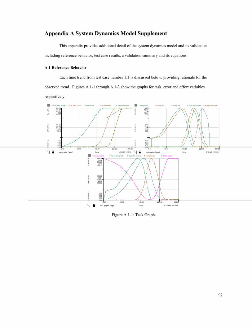
Appendix A System Dynamics Model Supplement

This appendix provides additional detail of the system dynamics model and its validation

including reference behavior, test case results, a validation summary and its equations.

A.1 Reference Behavior

Each time trend from test case number 1.1 is discussed below, providing rationale for the

observed trend. Figures A.1-1 through A.1-3 show the graphs for task, error and effort variables

respectively.

8:18 AM 11/3/28Days 8:18 AM 11/3/28

0.00 75.00 150.00 225.00 300.00

Days

1:

1:

1:

2:

2:

2:

3:

3:

3:

4:

4:

4:

5:

5:

5:

0.00

2.63

5.26

0.00

5.14

10.27

0.00

5.74

11.48

0.00

5.14

10.27

0.00

2.63

5.26

1: design rate 3: testing rate 4: code inspection r…

task graphs: Page 2

8:18 AM 11/3/28

0.00 75.00 150.00 225.00 300.00

Days

1:

1:

1:

2:

2:

2:

3:

3:

3:

4:

4:

4:

5:

5:

5:

0.00

266.65

533.30

0.00

26.04

52.08

0.00

203.47

406.95

0.00

49.72

99.43

0.00

266.63

533.27

1: requirements 2: tasks designed 3: tasks for coding 5: tasks tested

1

1

1

1

2

2

2

2

3

3

3

34 4

4

45 5

5

5

task graphs: Page 3

0.00 75.00 150.00 225.00 300.00

1:

1:

1:

2:

2:

2:

3:

3:

3:

4:

4:

4:

5:

5:

5:

0.00

266.65

533.30

0.00

266.63

533.27

0.00

266.63

533.27

0.00

0.50

1.00

0.00

130.12

260.25

1: cum tasks design… 3: tasks tested 5: actual completio…2: cum tasks coded 4: fraction done 2: coding rate 5: design inspection…

1

1

1

12 2

2

23 3 3 34 4

4

4

5

5

5 5

4: tasks coded

1

1

1

1

2 2

2

2

3 3 3

3

4 44

4

5 5

5

5

task graphs: Page 1

Figure A.1-1: Task Graphs

92

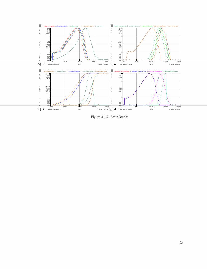
8:18 AM 11/3/28

0.00 75.00 150.00 225.00 300.00

Days

1:

1:

1:

2:

2:

2:

3:

3:

3:

4:

4:

4:

0.00

1.58

3.16

0.00

4.31

8.63

0.00

9.67

19.34

2: design error pass and a…3: code error escape rate 4: testing detection and c…

1

1

1

1

2

22

23 3

3

34 4

4

4

error graphs: Page 4

8:18 AM 11/3/28

0.00 75.00 150.00 225.00 300.00

Days

1:

1:

1:

2:

2:

2:

3:

3:

3:

4:

4:

4:

5:

5:

5:

0.00

3.95

7.89

0.00

2.37

4.74

0.00

39.06

78.12

0.00

23.83

47.66

0.00

188.83

377.66

2: design error dete… 3: design errors 5: code errors1: design error gener…

1: design error escape rate

4: detected design e… 4: design rework rate 5: code rework rate

1 1

1

1

2 2

2

23 3

3

3

4

4

4 45 5

5

5

1: undetected desig… 5: errors fixed in test

1

1

1

1

2 2

2

23

3

33

4 4

4

4

5 5

5

5

1

1

1

1

2

22

2

3

3

3

3

4

4

4 4

5

5

5

5

error graphs: Page 1 8:18 AM 11/3/28

0.00 75.00 150.00 225.00 300.00

Days

1:

1:

1:

2:

2:

2:

3:

3:

3:

4:

4:

4:

5:

5:

5:

0.00

7.70

15.41

0.00

66.05

132.11

0.00

6.47

12.94

0.00

2.38

4.77

0.00

6.61

13.21

1: code error genera…2: detected code err… 3: code error detect…

error graphs: Page 2

8:18 AM 11/3/28

0.00 75.00 150.00 225.00 300.00

Days

1:

1:

1:

2:

2:

2:

3:

3:

3:

4:

4:

4:

5:

5:

5:

0.00

159.99

319.98

0.00

106.25

212.50

0.00

239.98

479.97

0.00

334.79

669.58

0.00

223.19

446.39

2: escaped errors 3: reworked design … 4: reworked code er…

error graphs: Page 3

Figure A.1-2: Error Graphs

93

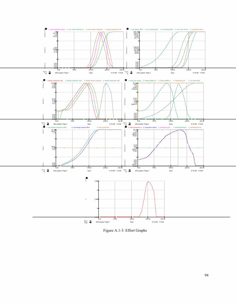
8:18 AM 11/3/28

0.00 75.00 150.00 225.00 300.00

Days

1:

1:

1:

2:

2:

2:

3:

3:

3:

4:

4:

4:

0.00

0.98

1.95

0.00

50.66

101.32

0.00

0.73

1.45

0.00

11.79

23.58

1: code inspection manpo… 2: cum code inspection e… 3: code rework manpowe… 4: coding manpower rate

1 1

1

1

2 2

2

2

3 3

3

34 4

4

4

5: cumulative test e…

1

1

1

1

2 2

2

2

3 3 3

3

4 4

4

4

5 5

5

5

3: design rework manpow… 4: manpower pool

3: max productivity

1

1

1

1

2

2

2

2

3 3 3 3

5: estimated test sc…

1

1

1

1

2

2

2

2

3 3 3 3

4 4 4 4

5 5

5 5

effort graphs: Page 1 8:18 AM 11/3/28

0.00 75.00 150.00 225.00 300.00

Days

1:

1:

1:

2:

2:

2:

3:

3:

3:

4:

4:

4:

5:

5:

5:

0.00

1046.00

2091.99

0.00

612.09

1224.17

0.00

287.33

574.65

0.00

36.83

73.65

0.00

128.56

257.12

1: cum design effort 2: cum coding effort 3: cum testing effort 4: cum code rework…

effort graphs: Page 2

8:18 AM 11/3/28

0.00 75.00 150.00 225.00 300.00

Days

1:

1:

1:

2:

2:

2:

3:

3:

3:

4:

4:

4:

0.00

10.32

20.64

0.00

0.50

1.00

0.00

0.13

0.26

0.00

6.12

12.24

2: design inspection man… 4: testing manpower rate1: design manpower rate

1: total manpower ra…

1: test staff curve

1 1 1

1

8:18 AM 11/3/28

0.00 75.00 150.00 225.00 300.00

Days

1:

1:

1:

2:

2:

2:

3:

3:

3:

4:

4:

4:

5:

5:

5:

0.00

47.20

94.39

0.00

0.44

0.87

0.00

0.50

1.00

0.00

11.80

23.60

0.00

2096.76

4193.52

1: hiring and manpo… 2: design staffing cu… 3: coding staffing c… 5: cum total effort

1 1 1 1

2

2

2

23 3

3

3

4 4 4 4

5

5

5

5

effort graphs: Page 4

1

1

1

1

2

22

2

3

3

3

34 4

4

4

effort graphs: Page 3

8:18 AM 11/3/28

0.00 75.00 150.00 225.00 300.00

Days

1:

1:

1:

2:

2:

2:

3:

3:

3:

0.00

50.66

101.33

0.00

13.20

26.40

-0.88

0.12

1.12

1: cum design inspection effort 2: cum design rework effort

effort graphs: Page 5

8:18 AM 11/3/28

0.00 75.00 150.00 225.00 300.00

Days

1:

1:

1:

0.00

0.42

0.85

effort graphs: Page 7

8:18 AM 11/3/28

0.00 75.00 150.00 225.00 300.00

Days

1:

1:

1:

2:

2:

2:

3:

3:

3:

4:

4:

4:

5:

5:

5:

0.00

13.20

26.41

0.00

0.56

1.12

0.00

11.80

23.60

284.07

285.07

286.07

66.88

72.98

79.09

2: manpower utilizat… 3: manpower pool 4: estimated develo…

effort graphs: Page 6

Figure A.1-3: Effort Graphs

94

task graphs: Page 1

This graph presents a high level overview of project progress, including cumulative depictions of task

progress for the main activities of design, code and test; fraction done; and completion time.

1: cum tasks designed

The cumulative tasks designed is monotonically increasing while design is taking place and levels off as

design completes. Since the design rate builds up and decreases, it exhibits an s-shaped behavior. This

shape is consistent with progress tracking charts from projects that have similar staffing patterns. With a

constant design rate, it would be a perfect ramp.

2: cum tasks coded

The cumulative tasks coded is monotonically increasing while coding is taking place and levels off as

coding completes. It also exhibits an s-shaped behavior due to the escalation and declination in the rate of

coding.

3: cum tasks tested

The cumulative tasks tested is monotonically increasing while testing is taking place and levels off as

testing completes. It also exhibits an s-shaped behavior due to the escalation and declination in the rate of

testing.

4: fraction done

The fraction done is the ratio of tasks tested to job size, indicating project completion percentage and is

monotonically increasing. Scaled independently, it properly matches the curve for cumulative tasks tested

and is coincident.

4: actual completion time

95

The actual completion time is a cycle time utility that instruments the maximum time of tasks in-process

that are time-stamped at requirements generation rate and complete testing. It’s final value indicates the

project’s actual schedule time. It is a ramp once testing commences since it measuring the maximum time

in process of all tasks that have completed testing up to that point.

task graphs: Page 2

These curves show the rates of various lifecycle activities in terms of tasks/day.

1: design rate

The design rate is influenced by the amount of personnel devoted to it and the fluctuation in productivity.

It follows the staffing profile policy input which is a Rayleigh-like curve. Productivity remains constant in

this test case for ease of analysis.

2: coding rate

The coding rate is influenced primarily by the amount of personnel devoted to it, and secondarily by the

fluctuation in productivity. It follows the staffing profile policy input which is a Rayleigh-like curve.

3: testing rate'

It follows the test staffing Rayleigh-like curve. Productivity remains constant in this test case for ease of

analysis.

4: code inspection rate

As seen in the curve, code inspection is set with a delay of 10 days after coding. It also has the same

magnitude of coding in tasks/day since this test case simulates 100% inspections performed and inspection

tasks do not fall behind.

5: design inspection rate

96

Similar to the code inspection rate, design inspection is set with a delay of 10 days after design and also

has the same magnitude as the design curve.

task graphs: Page 3

This graph shows the levels of tasks as they progress through phases in the development process.

1: requirements

The level of requirements is initiated with a pulse of magnitude job size at time zero. It then declines in a

manner converse to the cumulative tasks designed, and reaches zero when all tasks have been designed.

2: tasks designed

The tasks designed increases as design starts, and the rate of increase slows as design gives way to coding.

Tasks transition to the state of tasks in coding after they are inspected. The sharp angle at the beginning is

due to inspections starting to take place, thus the outgoing rate starts to increase and tasks enter the “tasks

for coding” state.

3: tasks in coding

Tasks in coding represents the intermediate state between design and tasks coded. It builds up as tasks

finish design, and decreases when more tasks are being coded than designed.

4: tasks coded

The tasks in coding increases as coding starts, and the rate of increase slows as coding gives way to testing.

Tasks transition to tasks ready for test after they are inspected.

5: tasks tested

Same as tasks tested on page 1 of the task graphs.

97

error graphs: Page 1

This graph depicts design error levels, design error rates and code errors.

1: design error generation rate

The design error generation rate is slaved to the design rate, since it is a co-flow. It is seen that its

magnitude is properly 1.5 times the design rate shown in the task graphs.

2: design error detection rate

The design error detection rate is slaved to the level of design errors shown in curve 3, and its magnitude is

determined by the efficiency of inspections. It is seen that its magnitude is 60% of the level of design

errors, as expected since the detection efficiency is .6.

3: design errors

Since design errors are generated simultaneously as a co-flow of design, its curve shape matches the level

of design tasks. Its magnitude is determined by the rate of design error generation. As design inspections

are performed, they transition to the detected or undetected state.

4: detected design errors

The detected design errors rise as design inspections are performed, and decrease as they are reworked.

The early hump is a start-up artifact of the delay for inspections (ingoing rate) compounded with the fixed

delay for rework (outgoing rate), and causes humps in downstream related variables such as rework effort.

5: code errors

The level of code errors represents errors in code before inspection. It is fed by a co-flow of coding as well

as the passing and amplification of undetected design errors. As code inspections are performed, they

transition to the detected or undetected state.

98

error graphs: Page 2

This graph shows the rates and levels of code errors in various states, as well as the design rework rate.

1: code error generation rate

The code error generation rate is linearly related to the coding rate, since error production is a co-flow of

coding. It properly matches the shape of the coding rate curve, and the magnitude is seen to be correct at

1.5* coding rate.

2: detected code errors

The detected code errors rise as code inspections are performed, and decrease as they are reworked since

this represents code errors detected during inspection before rework occurs.

3: code error detection rate

The code error detection rate is slaved to the level of code errors, and its magnitude is determined by the

efficiency of inspections. It is seen that its magnitude is 60% of the level of code errors, as expected since

the detection efficiency is .6.

4: design rework rate

Design error rework follows inspection by 10 days, and thus the rate follows the level of detected design

errors with the proper delay.

5: code rework rate

Code error rework follows inspection by 10 days, and thus the rate follows the level of detected code errors

with the proper delay.

error graphs: Page 3

This graph shows cumulative levels of errors, except for non- cumulative escaped errors.

99

1: undetected design errors

The level of undetected design errors rises with the generated design errors. This cumulative depiction

instruments the total number of design errors undetected during inspection which are passed and amplified

to the coding phase. Its final magnitude is correct as the total number of design errors multiplied by (1-

inspection efficiency).

2: escaped errors

The level of escaped errors rises as code inspections complete, but then starts falling as testing activities

detect and fix them. The level reaches zero as testing completes.

3: reworked design errors

The level of design errors reworked due to inspection is monotonically increasing from design inception

until design completes.

4: reworked code errors

The level of code errors reworked due to inspection is monotonically increasing from coding inception

until coding completes.

5: errors fixed in test

The level of errors detected and fixed during testing is cumulative as testing takes place.

error graphs: Page 4

This graph shows various rates of error escape, passage through phases and detection.

1: design error escape rate

100

The rate of design errors escaping to coding follows the level of design errors, as multiplied by (1-

inspection efficiency).

2: design error pass and amplification rate

The pass and amplification rate of design errors to code errors is linearly related to the design error escape

rate, as multiplied by the average design error amplification. It peaks and drops since error generation

occurs simultaneously as tasks are designed, which is a similar curve as seen in the task graphs.

3: code error escape rate

The rate of code errors escaping to test follows the level of code errors, as multiplied by (1- inspection

efficiency).

4: testing detection and correction rate

The testing detection and correction rate is implemented as a delay from escaped errors equivalent to the

estimated duration for testing.

effort graphs: Page 1

The graph shows some coding manpower rates and cumulative code inspection effort.

1: code inspection manpower rate

The code inspection manpower rate equals the rate of code inspection multiplied by the inspection effort

per task, and is seen to match the curve of code inspection rate and scaled accordingly by the effort per

task.

2: cum code inspection effort

The cumulative code inspection effort continues to increase monotonically as code inspection are

performed.

101

3: code rework manpower rate

The code rework manpower rate rises as code errors are detected, and falls as they are reworked.

4: coding manpower rate

The coding manpower rate follows the coding staffing profile curve seen in page 4 of the effort graphs,

with the magnitude determined by the manpower pool.

effort graphs: Page 2

All the curves on this chart are cumulative effort.

1: cum design effort

The cumulative design effort is monotonically increasing while design takes place.

2: cum coding effort

The cumulative code effort is monotonically increasing while coding takes place.

3: cum testing effort

The cumulative testing effort is monotonically increasing while testing takes place.

4: cum code rework effort

The cumulative code rework effort is monotonically increasing while code errors are reworked.

effort graphs: Page 3

This graph shows more manpower rates for various development activities.

1: design manpower rate

102

The design manpower rate follows the design staffing profile curve seen in page 4 of the effort graphs,

with the magnitude determined by the manpower pool.

2: design inspection manpower rate

The design inspection manpower rate equals the rate of design inspection multiplied by the inspection

effort per task, and is seen to match the curve of design inspection rate and scaled accordingly by the effort

per task.

3: design rework manpower rate

The design rework manpower rate rises as design errors are detected, and falls as they are reworked.

4: testing manpower rate

The testing manpower rate has two components: the fixed portions for test planning and execution, and the

variable component of error detection and correction. It is proportional to the test staffing curve, and

multiplied by the manpower allocation.

effort graphs: Page 4

This effort graph shows manpower allocation policies and cumulative total effort.

1: hiring and manpower allocation

The hiring and manpower allocation is a pulse as determined by project size, schedule and staff

productivity. It occurs at time zero only. Since the DT time increment is equal to .25 for the simulation,

the pulse magnitude is four times the allocated staff size.

2: design staffing curve

The design staffing curve is a Rayleigh-like curve that peaks and subsides during the initial part of

development, expressed as a fraction of the available personnel.

103

3: coding staffing curve

The coding staffing curve is a Rayleigh-like curve that peaks and subsides, starting after design with the

proper phase delay and expressed as a fraction of the available personnel.

4: manpower pool

The manpower pool represents the level of available personnel that were pulsed in by the hiring and

manpower allocation rate at time zero. It stays constant with the zero attrition.

5: cum total effort

The cumulative total effort of all activities is monotonically increasing from design inception until the last

task is tested.

effort graphs: Page 5

This graph shows some cumulative effort curves. Some variables for debugging purposes only are not

discussed.

1: cum design inspection effort

The cumulative design inspection effort is monotonically increasing from design inception until the end of

design. It exhibits s-shaped behavior due to the peaked curve of design manpower rate.

2: cum design rework effort

The cumulative design rework effort follows the shape of cumulative design inspection effort since they

are directly correlated with each other with a short delay.

effort graphs: Page 6

This graph shows the project-wide effort curve and manpower utilization.

104

1: total manpower rate

The total manpower rate is a sum of all the other manpower rates. It approximates the intended Rayleigh-

like staffing curve, and is seen to be the correct sum of all activities.

2: manpower utilization

The manpower utilization is a ratio of the total manpower rate to the manpower pool, and the shape is

necessarily coincident with the total manpower rate. It is slightly greater than one because the inspection

manpower is not allotted in the initial staffing curves (calibrated to zero inspections).

effort graphs: Page 7

This graph shows the project-wide effort curve and manpower utilization.

1: test staffing curve

The test staffing curve is a Rayleigh-like curve that peaks and subsides, starting after coding with the

proper phase delay and expressed as a fraction of the available personnel. It is scaled for the error density.

105

A.2 Test Case Results Parameter settings and cumulative results from the simulation test cases are shown in Table A.2-1.

Values are in simulation units: job size is in tasks, effort is in person-days and schedule is in days. To

convert to other units use 60 SLOCS/task for size, 20 person-days per person-month for effort and 20 days

per calendar month.

106

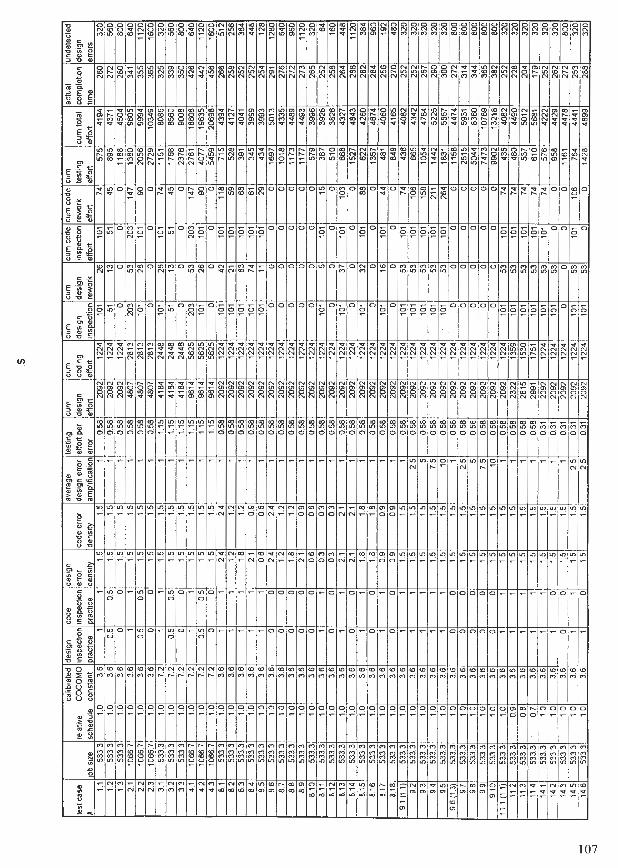
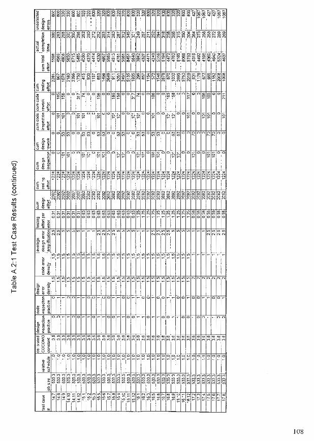
A.3 Validation Summary A summary of model validation follows in the sections below, drawing upon the test cases

demonstrated in Chapter 5 and the reference behavior results in section A.1 to judge the model against the

suite of validation tests shown in Table 5-1.

Test SS1 - dimensional consistency

The dimensions of the variables in each equation agree with the computation. Simulation time units are

days, the units for job size are tasks and effort is in person-days. Appropriate conversions between months

and days are documented in the source code (see section A.4). The defect density is measured in

defects/task converted from defects/KSLOC, with conversions also documented in the source code.

SS2 - extreme conditions in equations

Extreme conditions in equations have been tested by varying job size, productivity, error generation rates,

defect density, error multiplication and process delays. Job size has varied from very small (2 KSLOC) to

the high end of the middle-large project size region (128 KSLOC). The simulation has remained stable

under these conditions, with some fluctuating behavior seen with extreme process delays.

Test SS3 - boundary adequacy

Refer to Figure 3.4-3 for the model boundary definition. The structural boundary does contain the

variables and feedback loops to investigate the aforementioned aspects of the inspection process, and

eliminates effects that would confound the inspection analysis. Policy levers include various process

parameters, where managerial decision policies control their settings. These include appropriating the

amount of effort put into inspections, whether or not manpower constraints are employed, and dictating

schedule constraints. It is seen that varying the amount of effort on inspections has important effects on

product quality and project cost.

Test CS1 - face validity

109

The model structure matches the real system in terms of tasks, error flow and manpower utilization. Face

validity of constructs is checked against experts, other software practitioners, written sources and personal

experience. Face validity has been verified by international experts in relevant areas including system

dynamics, cost estimation, process technology and inspections. The overall effect of inspections

corroborates a good deal of published data, and inspection delays are consistent with experience. The

effect of inspections matches Fagan’s generalized curve fairly well. His testing peak is greater than that in

the COCOMO model, and is not literally meant to be an effort estimation curve.

Test CS2 - parameter values

Default assignment of parameters are documented in the source code shown in section A.4. All available

data on inspections was used to assign parameter values.

Test US1 - appropriateness of model characteristics for audience

Refer to the initial goals of the modeling experiment. The model is appropriate for examining defect

finding rates from inspections, the resulting escaped and reworked errors and the associated efforts. Effort

for specific activities available from the simulation is also consistent with the stated goals of the research

identified in Chapter 3. A managerial audience wants to see the impact of using inspections or not, and the

relative process efficiency of varying the inspection effort in different phases.

Test SB1 - parameter (in)sensitivity

In this test, the sensitivity of behavior characteristics to parameter changes is examined as well as policy

conclusions. The following parameters are used to evaluate model sensitivity: job size, workforce

available, defect density, staffing curves, error multiplication, and others. The results of these tests are

detailed in Chapter 5. The resulting project cost, duration and/or error levels varied as expected when

varying these parameters. Policy insight is afforded based on the sensitivity tests.

Test SB2 - structural (in)sensitivity

110

Sensitivity of behavior characteristics to structural formulations was gauged during model development.

Overall, the model behavior is stable with minor perturbations in the structure. For example, certain delays

were also represented as dependent on successor levels instead of the rates going into those levels. The

major instance of this was for defining the inspection rate as a delay from the level of designed/coded tasks

versus a fixed delay from the design/coding rates. The resultant behavior was less smooth, or “non-ideal”

because of minor fluctuations, but cumulative results stayed the same. It is arguable whether such

structures are more realistic since they better approximate true state transitions, but the chosen structure is

easier to assess simulation behavior because it is a smoothed version of the fluctuating behavior and

provides equivalent cumulative results.. Policy conclusions should not change drastically with minor

changes in structure.

Test CB1 - replication of reference modes (boundary adequacy for behavior)

See the section A.1 on reference behavior. The model endogenously reproduces behavior modes initially

defined in the study in terms of past policies and anticipated behavior.

Test CB2 - surprise behavior

Little surprise behavior has been noted. See the discussion for test SB2 above on fluctuating trends. These

trends were initially a surprise, but investigation showed them to be realistic. For example, personnel often

save up certain tasks until a threshold is reached, and then spend time on the saved up tasks. For instance,

the average developer does not spend some time each day on programming and inspection preparation.

Instead, he prepares for inspection when it is time to do so, and then spends nearly full-time on that until

it’s finished. Other surprise results was that inspections were not cost effective for certain organizations

where the cost of fixing defects during test was less than the cost of inspections. This is one insight of the

model; that under certain conditions inspections are not worthwhile.

Test CB3 - extreme condition simulations

111

Extreme condition simulations were performed, as identified in the SS2 validation tests. The model

formulation is sensible, since the model behaved well under extreme conditions.

Test CB4 - statistical tests

As demonstrated in Chapter 5, various statistical tests were performed. The model output statistically

matched real system data in terms of inspection and rework effort, error rates, schedule performance,

overall effort and inspection return on investment. See section 5.5 for validation of the model against

industrial data.

Test UB1 - counter-intuitive behavior

Counter-intuitive behavior demonstrated was the diminishing returns of inspections, as noted in the CB2

test above.

Test UB2 - generation of insights

The model has provide several insights into the dynamic effects of inspections on the development process.

One insight is that inspections are worthwhile under certain project conditions. Besides when inspection

efficiency is reduced, inspections are not necessarily cost-effective if the organization can find and fix

defects cheaply during the testing phase. Also, depending on the error multiplication rate, design

inspections are more cost effective than code inspections.

A.4 Equations

Table A.4-1 lists the underlying equations for the model diagram shown in Figure 3.4-1

supplemented with documentary comments for each equation. Comments describe the variables, provide

units and identify assumptions used in the formulations.

112

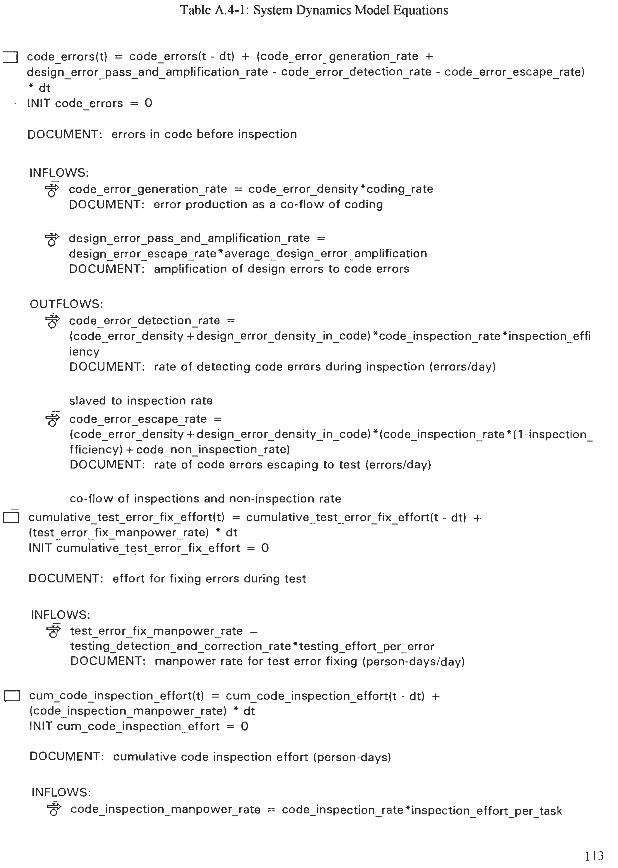
Table A.4- 1 : System Dynamics Model Equations

n code-errors(t) = code-errors(t - dt) + (code-error-generation-rate + des ign~error~pass~and~ampl i f icat ion~rate - code-error-detection-rate - code-error-escape-rate) * d t INIT code-errors = 0

DOCUMENT: errors in code before inspection

INFLOWS: code-error-generation-rate = code-error-density *coding-rate DOCUMENT: error production as a co-flow of coding

3 design-error-pass-and-amplification-rate = design-error-escape-rate *average-design-error-amplification DOCUMENT: amplification of design errors to code errors

OUTFLOWS: $ code-error-detection-rate =

(code - error-density + design-error-density-in-code) *code~inspect ion~rate* inspect ion~ef f i iency DOCUMENT: rate of detecting code errors during inspection (errorslday)

slaved to inspection rate

$ code-error-escape-rate = (code-error-density + design-error-density-in-code) *(code-inspection-rate * ( 1 -inspection- fficiency) + code-non-inspection-rate) DOCUMENT: rate of code errors escaping to test (errorslday)

co-flow of inspections and non-inspection rate

0 cumula t i ve~ tes t~er ro r~ f i x~e f fo r t ( t ) = cumula t i ve~ tes t~er ro r~ f i x~e f fo r t ( t - dt) + (test-error-fix-manpower-rate) * d t INIT cumula t i ve~ tes t~er ro r~ f i x~e f fo r t = 0

DOCUMENT: effort for fixing errors during test

INFLOWS: $ test-error-fix-manpower-rate =

testing-detection-and-correction-rate "testing-effort-per-error DOCUMENT: manpower rate for test error fixing (person-dayslday)

0 cum~code~inspect ion~ef for t ( t ) = cum~code~ inspec t ion~e f fo r t ( t - dt) + (code~inspect ion~manpower~rate) * d t INIT cum~code~ inspec t ion~e f fo r t = 0

DOCUMENT: cumulative code inspection effort (person-days)

INFLOWS: $ code~ inspec t i on~manp~wer~ ra te = code~inspect ion~rate* inspect ion~ef for t~per~task

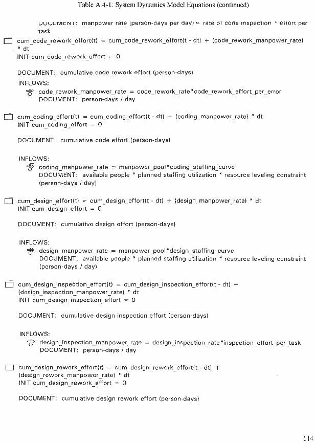
Table A.4-1: System Dynamics Model Equations (continued)

UULUIVI~IV I : manpower rare (person-aays per aayt = rare or coae mspecrlon - errorr per task

cum~code~rework~ef fo r t ( t ) = cum-code-rework-effort(t - dt) + (code-rework-manpower-rate) * d t INIT c u m ~ c o d e ~ r e w o r k ~ e f f o r t = 0

DOCUMENT: cumulative code rework effort (person-days)

INFLOWS: 3 code-rework-manpower-rate = code~ rewo rk~ ra te *code~ rewo rk~e f f o r t ~pe r~e r ro r

DOCUMENT: person-days / day

0 cum-coding-effort(t) = cum-coding-effort(t - dt) + (coding-manpower-rate) * d t INIT cum-coding-effort = 0

DOCUMENT: cumulative code effort (person-days)

INFLOWS: 3 coding manpower-rate = manpower~pool*coding~staffing~curve

DOCUMENT: available people * planned staffing utilization * resource leveling constraint (person-days / day)

0 cum-design-effort(t) = cum-design-effort(t - dt) + (design-manpower-rate) * d t INIT cum-design-effort = 0

DOCUMENT: cumulative design effort (person-days)

INFLOWS: 3 design-manpower-rate = manpower~pool*design~staffing_curve

DOCUMENT: available people * planned staffing utilization * resource leveling constraint (person-days / day)

0 cum~design~inspection_effort(t) = cum-design-inspection-effort(t - dt) + (design-inspection-manpower-rate) * d t INIT cum~design~inspect ion~ef for t = 0

DOCUMENT: cumulative design inspection effort (person-days)

INFLOWS: 3 design-inspection-manpower-rate = design~inspection_rateXinspection~effort_per_task

DOCUMENT: person-days / day

cum-design-rework-effort(t) = cum-design-rework-effort(t - dt) + (design-rework-manpower-rate) * d t INIT cum-design-rework-effort = 0

DOCUMENT: cumulative design rework effort (person-days)

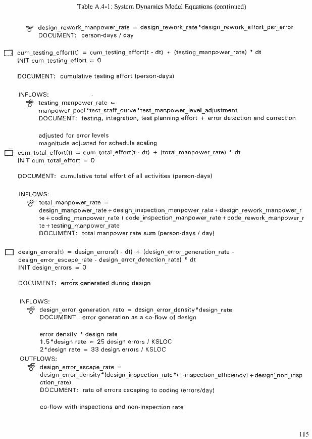
Table A.4-1: System Dynamics Model Equations (continued)

design-rework-manpower-rate = des ign~rework~ra te*des ign~rework~e f fo r t~per~er ro r DOCUMENT: person-days / day

0. cum-testing-effort(t) = cum-testing-effort(t - dt) + (testing-manpower - rate) * d t INIT cum-testing-effort = 0

DOCUMENT: cumulative testing effort (person-days)

INFLOWS: 3 testing-manpower-rate =

manpower-pool "test-staff-curve * test~manpower~level~adjustment DOCUMENT: testing, integration, test planning effort + error detection and correction

adjusted for error levels magnitude adjusted for schedule scaling

0 cum-total-effort(t) = cum-total-effort(t - dt) + (total-manpower-rate) * d t INIT cumtotal-effort = 0

DOCUMENT: cumulative total effort of all activities (person-days)

INFLOWS: 9 total-manpower-rate =

design-manpower-rate + design-inspection-manpower-rate + design-rework-manpower-r te + coding-manpower-rate + code~inspect ion~manpower~rate + code-rework-manpower-r te + testing-manpower-rate DOCUMENT: total manpower rate sum (person-days / day)

0 design-errors(t) = design-errors(t - dt) + (design-error-generation-rate - design-error escape-rate - design-error-detection-rate) * d t INIT design-errors = 0

DOCUMENT: errors generated during design

INFLOWS: 3 design-error-generation-rate = design-error-density 'design-rate

DOCUMENT: error generation as a co-flow of design

error density * design rate 1.5'design rate = 25 design errors / KSLOC 2'design rate = 33 design errors / KSLOC

OUTFLOWS: design-error-escape-rate = design-error-density *(design-inspection-rate '(I -inspection-efficiency) +design - non - insp ction-rate) DOCUMENT: rate of errors escaping to coding (errorslday)

co-flow with inspections and non-inspection rate

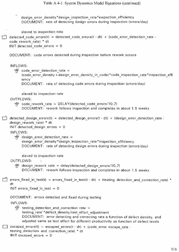
Table A.4-1: System Dynamics Model Equations (continued)

design-error-density "design-inspection-rate *inspection-efficiency DOCUMENT: rate of detecting design errors during inspection (errorslday)

slaved to inspection rate

0 detected-code-errordt) = detected-code-errors(t - dt) + (code-error-detection-rate - code-rework-rate) * d t INIT detected-code-errors = 0

DOCUMENT: code errors detected during inspection before rework occurs

INFLOWS: 3 code-error-detection-rate =

(code-error-density + design-error-density-in-code) *code-inspection-rate *inspection-effi iency DOCUMENT: rate of detecting code errors during inspection (errorslday)

slaved to inspection rate

OUTFLOWS: code-rework-rate = DELAY(detected-code-errors/l0,7) DOCUMENT: rework follows inspection and completes in about 1.5 weeks

0 detected - design-errors(t) = detected-design-errors(t - dt) + (design-error-detection-rate - design-rework-rate) * d t INIT detected-design-errors = 0

INFLOWS: 3 design-error-detection-rate =

design-error-density *design-inspection-rate *inspection-efficiency DOCUMENT: rate of detecting design errors during inspection (errorslday)

slaved to inspection rate

OUTFLOWS: 2

3 design-rework-rate = delay(detected-design-errorsll0,7) DOCUMENT: rework follows inspection and completes in about 1.5 weeks

0 errors-fixed-in-test(t) = errors-fixed-intest(t - dt) + (testing-detection-and-correction-rate) * d t INIT errors-fixed-in-test = 0

DOCUMENT: errors detected and fixed during testing

INFLOWS: 3 testing-detection-and-correction-rate =

test incrate' "defect-densityltest-effort-adjustment DOCUMENT: error detecting and correcting rate a function of defect density, and adjusted same as test effort for different productivity as function of defect levels

escaped-errors(t) = escaped-errors(t - dt) + (code-error-escape-rate - testing-detection-and-correction-rate) * d t INIT escaped-errors = 0

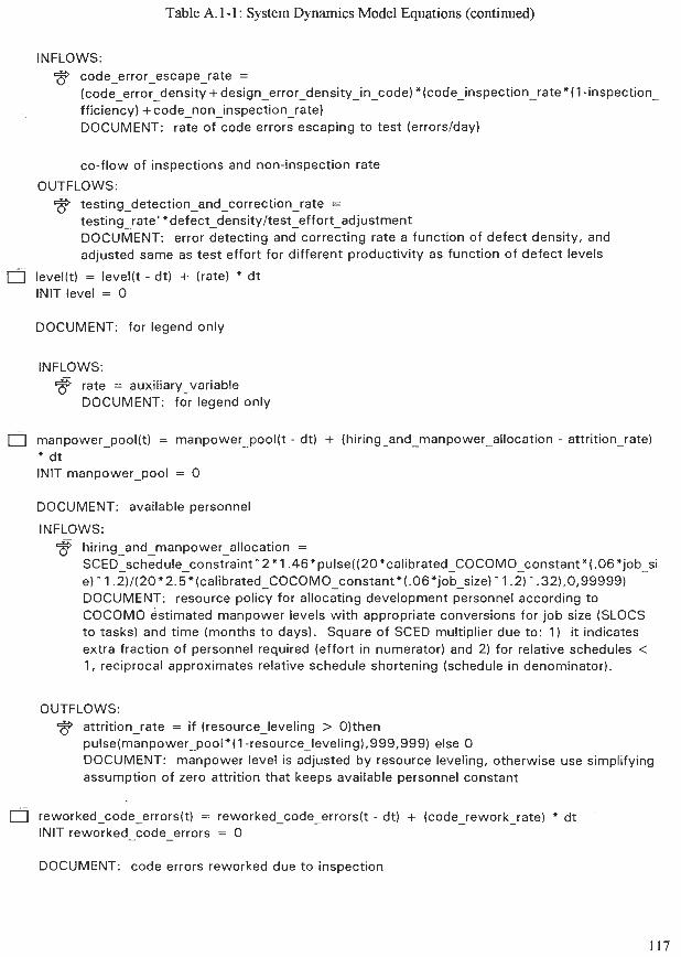
Table A. 1-1: System Dynamics Model Equations (continued)

INFLOWS: 3 code-error-escape-rate =

(code error - density + design-error-density-in-code) "(code-inspection-rateX( 1 -inspection- fficieLcy) + code-non-inspection-rate) DOCUMENT: rate of code errors escaping to test (errorstday)

co-flow of inspections and non-inspection rate

OUTFLOWS: @ testing-detection-and-correction-rate =

testing-rate' *defect~density/ test~effort~adjustment DOCUMENT: error detecting and correcting rate a function of defect density, and adjusted same as test effort for different productivity as function of defect levels

0 level(t) = ievel(t - dt) + (rate) * d t INIT level = 0

DOCUMENT: for legend only

INFLOWS: e rate = auxiliary-variable DOCUMENT: for legend only

0 manpower-pool(t) = manpower-pool(t - dt) + (hiring-and-manpowe * d t INIT manpower-pool = 0

in - attrition-rate)

DOCUMENT: available personnel

INFLOWS: 3 hiring-and-manpower-allocation =

SCED~schedu le~cons t ra in t~2*1 .46*pu lse ( (20*ca l ib ra ted~COCOMO~~ons tan t * ( .06* job~~ i e)-1.2)/(20*2.5*(calibrated - COCOMO constant*(.06*job~size)~1.2)~.32),0,99999) DOCUMENT: resource policy for alloc&ng development personnel according to COCOMO estimated manpower levels wi th appropriate conversions for job size (SLOCS to tasks) and time (months to days). Square of SCED multiplier due to: 1) it indicates extra fraction of personnel required (effort in numerator) and 2) for relative schedules < 1, reciprocal approximates relative schedule shortening (schedule in denominator).

OUTFLOWS: 9 attrition-rate = if (resource-leveling > 0)then

pulse(manpower-pool * ( I -resource-leveling),999,999) else 0 DOCUMENT: manpower level is adjusted by resource leveling, otherwise use simplifying assumption of zero attrition that keeps available personnel constant

0 reworked code errors(t) = reworked-code-errors(t - dt) + (code-rework-rate) l dt INIT reworked-code-errors = 0

DOCUMENT: code errors reworked due to inspection

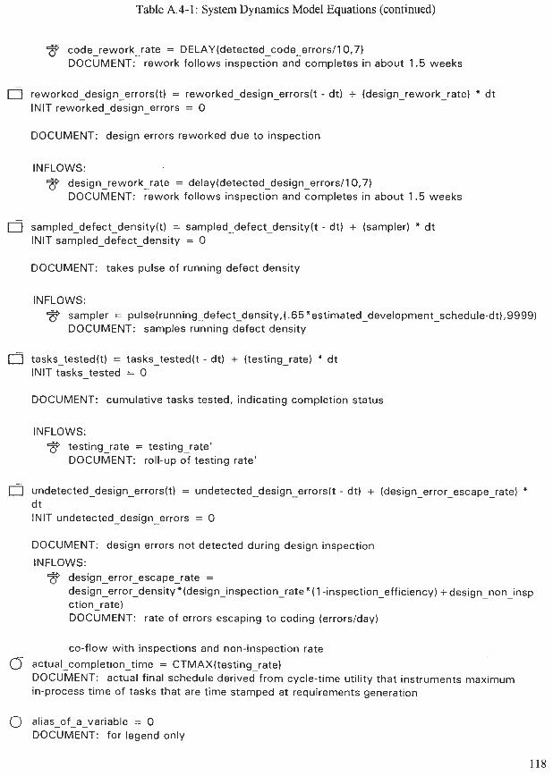
Table A.4-1: System Dynamics Model Equations (continued)

code rework-rate = DELAY(detected~code~errors/l0,7) DOCUMENT: rework follows inspection and completes in about 1.5 weeks

reworked design errors(t) = reworked-design-errors(t - dt) + (design-rework-rate) * d t INIT reworked-design-errors = 0

DOCUMENT: design errors reworked due to inspection

INFLOWS: 3 design-rework-rate = delay(detected-design~errors/l0,7)

DOCUMENT: rework follows inspection and completes in about 1.5 weeks

0 sampled-defect-density(t) = sampled-defect-density(t - dt) + (sampler) " d t INIT sampled-defect-density = 0

DOCUMENT: takes pulse of running defect density

INFLOWS: 3 sampler = pulse(running~defect~density,(.65*estimated~development~schedule-dt),9999)

DOCUMENT: samples running defect density

0 tasks-tested(t) = tasks-tested(t - dt) + (testing-rate) * d t INIT tasks-tested = 0

DOCUMENT: cumulative tasks tested, indicating completion status

INFLOWS: 3 testing-rate = testing-rate'

DOCUMENT: roll-up of testing rate'

0 undetected-design+errors(t) = undetected-design-errors(t - dt) + (design-error-escape-rate) * dt INIT undetected-design-errors = 0

DOCUMENT: design errors not detected during design inspection

INFLOWS: 3 design-error-escape-rate =

design-error-density "(design-inspection-rateX( 1 -inspection-efficiency) + design-non-insp ction-rate) DOCUMENT: rate of errors escaping to coding (errorslday)

co-flow with inspections and non-inspection rate

0 actual-completion-time = CTMAX(testing-rate) DOCUMENT: actual final schedule derived from cycle-time utility that instruments maximum in-process time of tasks that are time stamped at requirements generation

0 alias-of-a-variable = 0 DOCUMENT: for legend only

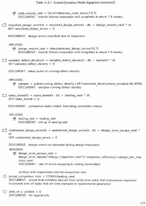
Table A.4-1: System Dynamics Model Equations (continued)

code-rework-rate = DELAY(detected~code~errors/ l0,7) DOCUMENT: rework follows inspection and completes in about 1.5 weeks

reworked - design-errors(t) = reworked-design-errors(t - dt) + (design-rework-rate) * d t INIT reworked-design-errors = 0

DOCUMENT: design errors reworked due to inspection

INFLOWS: 3 design-rework-rate = delay(detected~design~errors/l0,7)

DOCUMENT: rework follows inspection and completes in about 1.5 weeks

0 sampled-defect-density(t) = sampled-defect-density(t - dt) + (sampler) * d t INIT sampled-defect-density = 0

DOCUMENT: takes pulse of running defect density

INFLOWS: 3 sampler = pulse(running~defect~density,(.65*estimated~development~schedule-dt),9999)

DOCUMENT: samples running defect density

0 tasks tested(t) = tasks-tested(t - dt) + (testing-rate) * d t INIT tasks-tested = 0

DOCUMENT: cumulative tasks tested, indicating completion status

INFLOWS: 3 testing-rate = testing-rate'

DOCUMENT: roll-up of testing rate'

0 undetected - design+errors(t) = undetected-design-errors(t - dt) + (design-error-escape-rate) * d t INIT undetected-design-errors = 0

DOCUMENT: design errors not detected during design inspection

INFLOWS: 3 design-error-escape-rate =

design-error-density *(design-inspection-rate*( 1 -inspection-efficiency) +design - non - insp ction-rate) DOCUMENT: rate of errors escaping to coding (errorstday)

co-flow with inspections and non-inspection rate

0 actual-completion-time = CTMAX(testing-rate) DOCUMENT: actual final schedule derived from cycle-time utility that instruments maximum in-process time of tasks that are time stamped at requirements generation

0 alias-of-a-variable = 0 DOCUMENT: for legend only

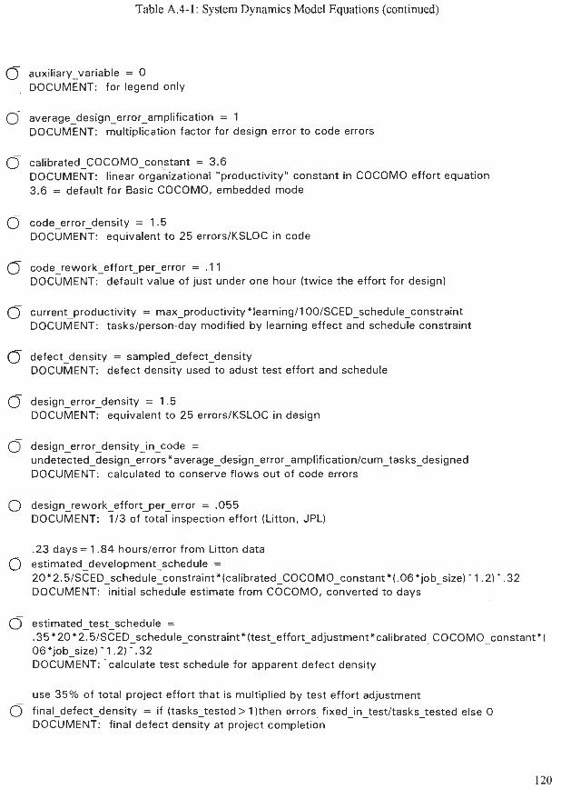
Table A.4-1: System Dynamics Model Equations (continued)

0 auxiliary-variable = 0 DOCUMENT: for legend only

0 average-design-error-amplification = 1 DOCUMENT: multiplication factor for design error to code errors

0 cal ibrated~COCOMO~constant = 3.6 DOCUMENT: linear organizational "productivity" constant in COCOMO effort equation 3.6 = default for Basic COCOMO, embedded mode

0 code-error-density = 1.5 DOCUMENT: equivalent to 25 errors1KSLOC in code

0 code-rework-effort-per-error = .I 1 DOCUMENT: default value of just under one hour (twice the effort for design)

0 current-productivity = max-productivity "learning11 00lSCED~schedule~constraint DOCUMENT: taskslperson-day modified by learning effect and schedule constraint

0 defect-density = sampled-defect-density DOCUMENT: defect density used to adust test effort and schedule

0 design-error-density = 1.5 DOCUMENT: equivalent to 25 errors1KSLOC in design

0 design-error-density-in-code = undetected-design-errors *average~design~error~ampl i f icat ionlcum~tasks~designed DOCUMENT: calculated to conserve flows out of code errors

0 design-rework-effort-per-error = .055 DOCUMENT: 113 of total inspection effort (Litton, JPL)

.23 days = 1.84 hourslerror from Litton data 0 estimated~development~schedule =

20*2.5/SCED~schedule~constraint*(cal ibrated~C0C0M0c0nstant*( .O6*job~size) I .2) .32 DOCUMENT: initial schedule estimate from COCOMO, converted to days

0 est imated~test~schedule =

.35 *20*2.5 /SCED~schedule~const ra in t * ( tes t~ef for t~ad jus tment*ca l ib ra ted~C0C0M0~c0nstant*~ 06"job-size) ^ I .2 ) " .32 DOCUMENT: 'calculate test schedule for apparent defect density

use 35% of total project effort that is multiplied by test effort adjustment

0 final-defect-density = if (tasks-tested > I )then e r ro rs~ f i xed~ in~ tes t l t asks~ tes ted else 0 DOCUMENT: final defect density at project completion

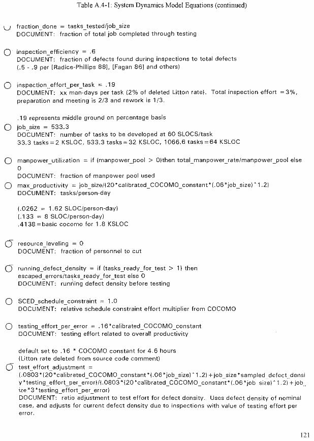
Table A.4-1: System Dynamics Model Equations (continued)

fraction-done = tasks-testedljob-size DOCUMENT: fraction of total job completed through testing

inspection-efficiency = .6 DOCUMENT: fraction of defects found during inspections to total defects (.5 - .9 per [Radice-Phillips 881, [Fagan 861 and others)

inspection-effort-per-task = .19 DOCUMENT: xx man-days per task (2% of deleted Litton rate). Total inspection effort =3%, preparation and meeting is 213 and rework is 113.

.I 9 represents middle ground on percentage basis

job-size = 533.3 DOCUMENT: number of tasks to be developed at 6 0 SLOCSItask 33.3 tasks = 2 KSLOC, 533.3 tasks = 32 KSLOC, 1066.6 tasks = 64 KSLOC

manpower - utilization = if (manpower-pool > 0)then total-manpower-ratelmanpower-pool else 0 DOCUMENT: fraction of manpower pool used

max productivity = job s i ze / (20*ca l i b ra ted~COCOMO~~0n~tan t * ( .06* job~s ize ) 1.2) DOCUMENT: taskslper;on-day

(.0262 = 1.62 SLOCIperson-day) (.I 33 = 8 SLOCIperson-day) .4138 =basic cocomo for 1.8 KSLOC

0 resource-leveling = 0 DOCUMENT: fraction of personnel to cut

0 running-defect-density = if (tasks-ready-for-test > I) then escaped-errorsltasks-ready-for-test else 0 DOCUMENT: running defect density before testing

SCED-schedule-constraint = 1.0 DOCUMENT: relative schedule constraint effort multiplier from COCOMO

0 testing-effort-per-error = .16*calibrated-COCOMO-constant DOCUMENT: testing effort related to overall productivity

default set to . I 6 * COCOMO constant for 4.6 hours (Litton rate deleted from source code comment) test-effort-adjustment = (.0803*(20*calibrated-COCOMO~constant*(.06*job-size) 1.2) + job-size*sampled-defect - densi y "testing - effort - per - error)/(.0803*(20*calibrated~COCOMO~constant*(.O6*job-size) I .2) +job- ize*3 *testing-effort-per-error) DOCUMENT: ratio adjustment to test effort for defect density. Uses defect density of nominal case, and adjusts for current defect density due to inspections with value of testing effort per error.

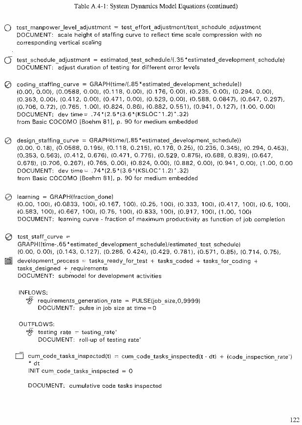
Table A.4-1: System Dynamics Model Equations (continued)

0 test-manpower-level-adjustment = test~effort~adjustment/ test~schedule~adjustment DOCUMENT: scale height of staffing curve to reflect time scale compression with no corresponding vertical scaling

0 test-schedule-adjustment = estimated~test~schedule/(.35*estimated~development~schedule) DOCUMENT: adjust duration of testing for different error levels

@ coding staffing curve = GRAPH(time/(.85'estimated~development~schedule)) (0.00, O.OO), (60588, O.OO), (0.1 1 8, O.OO), (0.1 76, O.OO), (0.235, O.OO), (0.294, O.OO), (0.353, O.OO), (0.41 2, O.OO), (0.471, O.OO), (0.529, O.OO), (0.588, 0.0847), (0.647, 0.297), (0.706, 0.72), (0.765, 1 .OO), (0.824, 0.861, (0.882, 0.551), (0.941, 0.127), (1 .OO, 0.00) DOCUMENT: dev time = .74*(2.5*(3.6*(KSLOC" 1.2) '.32) from Basic COCOMO [Boehm 811, p. 90 for medium embedded

@ design staffing curve = GRAPH(time/(.85*estimated~development~schedule~) (0 .00 , .18) , (6.0588, 0.195), (0.118, 0.215), (0.176, 0.25), (0.235, 0.345), (0.294, 0.453), (0.353, 0.563), (0.41 2, 0.676), (0.471, 0.775), (0.529, 0.875), (0.588, 0.839), (0.647, 0.678), (0.706, 0.267), (0.765, O.OO), (0.824, O.OO), (0.882, O.OO), (0.941, O.OO), (1 .OO, 0.00 DOCUMENT: dev time = .74*(2.5*(3.6*(KSLOC^ 1.2) .32) from Basic COCOMO [Boehm 811, p. 90 for medium embedded

@ learning = GRAPH(fraction-done) (0.00, 1 OO), (0.0833, 1001, (0.1 67, 1001, (0.25, 1001, (0.333, 1001, (0.41 7, 1001, (0.5, 1001, (0.583, IOO) , (0.667, 1001, (0.75, 1001, (0.833, 1001, (0.91 7, 1001, (1.00, 100) DOCUMENT: learning curve - fraction of maximum productivity as function of job completion

@ test-staff-curve = GRAPH((time-.65 *estimated~development~schedule)/estimated~test~schedule~ (0.00, O.OO), (0.143, 0.127), (0.286, 0.4241, (0.429, 0.781), (0.571, 0.85), (0.714, 0.75),

@ development-process = tasks-ready-for-test + tasks-coded + tasks-for-coding + tasks-designed + .requirements DOCUMENT: subhodel for development activities

INFLOWS: 3 requirements-generation-rate = PULSE(job_size,0,9999)

DOCUMENT: pulse in job size at time =O

OUTFLOWS: testing-rate = testing-rate' DOCUMENT: roll-up of testing rate'

0 cum~code~tasks~inspected( t ) = cum-code-tasks-inspected(t - dt) + (code-inspection-rate') * dt INIT cum~code~tasks~ inspec ted = 0

DOCUMENT: cumulative code tasks inspected

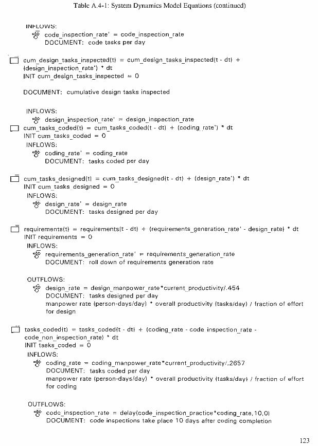
Table A.4-1: System Dynamics Model Equations (continued)

INI-LUWS:

5 code-inspection-rate' = code-inspection-rate DOCUMENT: code tasks per day

C ] cum~design~tasks~inspected(t) = cum~design~tasks~inspected(t - dt) + (design-inspection-rate') * d t INIT cum~design~tasks~inspected = 0

DOCUMENT: cumulative design tasks inspected

INFLOWS: 3 design-inspection-rate' = design-inspection-rate

0 cum tasks coded(t) = cum-tasks-coded(t - dt) + (coding-rate') * d t INIT~U~-tasks-coded = 0

INFLOWS: e coding-rate' = coding-rate DOCUMENT: tasks coded per day

0 cum-tasks-designed(t) = cum-tasks-designed(t - dt) + (design-rate') * d t INIT cum-tasks-designed = 0

INFLOWS: 3 design-rate' = design-rate

DOCUMENT: tasks designed per day

0 requirements(t) = requirementsct - dt) + (requirements-generation-rate' - design-rate) * dt INIT requirements = 0 INFLOWS: 5 requirements-generation-rate' = requirements-generation-rate

DOCUMENT: roll down of requirements generation rate

OUTFLOWS: 3 design-rate = design~manpower~rate*current~productivity/.454

DOCUMENT: tasks designed per day manpower rate (person-dayslday) * overall productivity (taskdday) 1 fraction of effort for design

0 tasks-coded(t) = tasks-coded(t - dt) + (coding-rate - code-inspection-rate -

code-non-inspection-rate) * d t INIT tasks-coded = 0

INFLOWS: 3 coding-rate = coding~manpower~rate*current~productivity/.2657

DOCUMENT: tasks coded per day manpower rate (person-dayslday) * overall productivity (taskslday) / fraction of effort for coding

OUTFLOWS: 9 code-inspectionrate = delay(code~inspect ion~pract ice*coding~rate, 10,O)

DOCUMENT: code inspections take place 1 0 days after coding completion

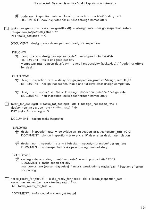
Table A.4-1: System Dynamics Model Equations (continued)

code-non-inspection-rate = (1 -code-inspection-practice) *coding-rate DOCUMENT: non-inspected tasks pass through immediately

0 tasks-designed(t) = tasks-designed(t - dt) + (design-rate - design-inspection-rate - design-non-inspection-rate) * d t INIT tasks-designed = 0

DOCUMENT: design tasks developed and ready for inspection

INFLOWS: 3 design-rate = design~rnanpower~rate*current~productivity/.454

DOCUMENT: tasks designed per day manpower rate (person-daystday) * overall productivity (taskdday) / fraction of effort for design

OUTFLOWS: 3 design-inspection-rate = delay(design-inspection-practice 'design-rate, l0,O)

DOCUMENT: design inspections take place 10 days after design completion

design-non-inspection-rate = (1 -design-inspection-practice) *design - rate DOCUMENT: non-inspected tasks pass through immediately

0 tasks - for - coding(t) = tasks-for-coding(t - dt) + (design-inspection-rate + design-non-inspection-rate - coding-rate) * d t INIT tasks-for-coding = 0

DOCUMENT: design tasks inspected

INFLOWS: 3 design-inspection-rate = delay(design-inspection-practice *design-rate, l0,O)

DOCUMENT: design inspections take place 10 days after design completion

3 design-non-inspection-rate = (1 -design-inspection-practice) +design-rate DOCUMENT: non-inspected tasks pass through immediately

OUTFLOWS: 3 coding-rate = coding~manpower~rate*current~productivity/.2657

DOCUMENT: tasks coded per day manpower rate (person-daystday) * overall productivity (taskstday) / fraction of effort for coding

0 tasks-ready-for-test(t) = tasks-ready-for-test(t - dt) + (code-inspection-rate + code-non-inspection-rate - testing-rate') d t INIT tasks-ready-for-test = 0

DOCUMENT: tasks coded and not yet tested

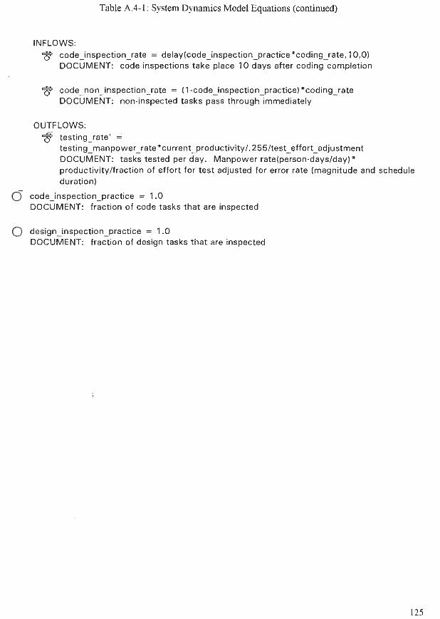
Table A.4-1: System Dynamics Model Equations (continued)

INFLOWS: code-inspection-rate = delay(code-inspection-practice *coding_rate, 0 , O ) DOCUMENT: code inspections take place 1 0 days after coding completion

code-non-inspection-rate = (1 -code-inspection-practice) *coding-rate DOCUMENT: non-inspected tasks pass through immediately

OUTFLOWS: 3 testing-rate' =

testing-manpower-rate *current~productivity/.255/test~effort~adjustment DOCUMENT: tasks tested per day. Manpower rate(person-daystday)* productivity/fraction of effort for test adjusted for error rate (magnitude and schedule duration)

0 code-inspection-practice = 1.0 DOCUMENT: fraction of code tasks that are inspected

0 design-inspection-practice = 1.0 DOCUMENT: fraction of design tasks that are inspected