A Software Deﬁned Networking evaluation approach to ...

A Software DefinedNetworking evaluationapproach to distributing loadUsing POX, Floodlight and BIG-IP 1600

Emil Sylvio GolinelliMaster’s Thesis Spring 2015

A Software Defined Networking evaluationapproach to distributing load

Emil Sylvio Golinelli

May 18, 2015

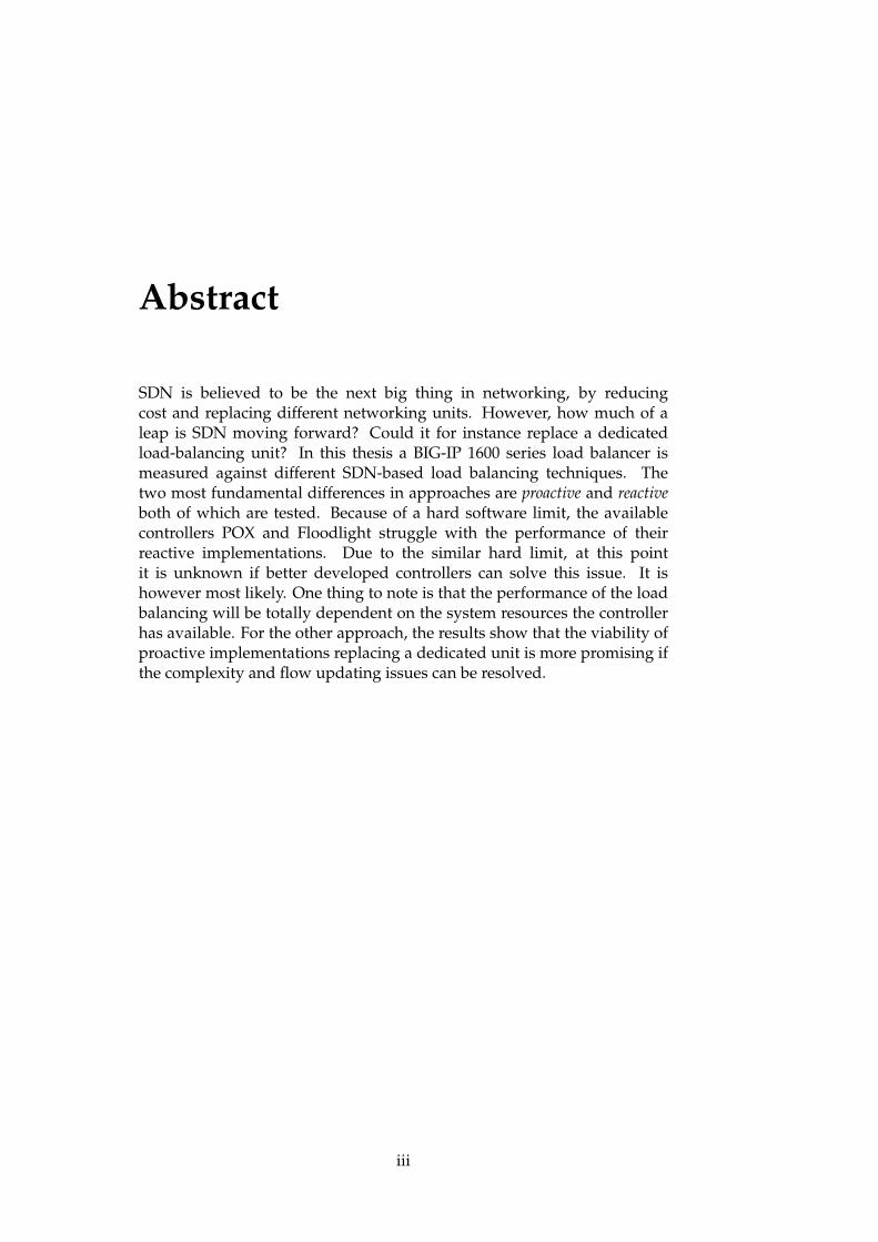
Abstract

SDN is believed to be the next big thing in networking, by reducingcost and replacing different networking units. However, how much of aleap is SDN moving forward? Could it for instance replace a dedicatedload-balancing unit? In this thesis a BIG-IP 1600 series load balancer ismeasured against different SDN-based load balancing techniques. Thetwo most fundamental differences in approaches are proactive and reactiveboth of which are tested. Because of a hard software limit, the availablecontrollers POX and Floodlight struggle with the performance of theirreactive implementations. Due to the similar hard limit, at this pointit is unknown if better developed controllers can solve this issue. It ishowever most likely. One thing to note is that the performance of the loadbalancing will be totally dependent on the system resources the controllerhas available. For the other approach, the results show that the viability ofproactive implementations replacing a dedicated unit is more promising ifthe complexity and flow updating issues can be resolved.

iii

Contents

I Introduction 1

1 Introduction 31.1 Motivation . . . . . . . . . . . . . . . . . . . . . . . . . . . . . 31.2 Problem Statement . . . . . . . . . . . . . . . . . . . . . . . . 41.3 Thesis Structure . . . . . . . . . . . . . . . . . . . . . . . . . . 51.4 Related Work . . . . . . . . . . . . . . . . . . . . . . . . . . . 6

1.4.1 OpenFlow-Based Server Load Balancing Gone Wild . 61.4.2 OpenFlow Based Load Balancing . . . . . . . . . . . . 61.4.3 Aster*x: Load-Balancing as a Network Primitive . . . 61.4.4 Load Balancing in a Campus Network using Soft-

ware Defined Networking . . . . . . . . . . . . . . . . 7

2 Background 92.1 The OSI model . . . . . . . . . . . . . . . . . . . . . . . . . . . 9

2.1.1 Layer 1 . . . . . . . . . . . . . . . . . . . . . . . . . . . 92.1.2 Layer 2 . . . . . . . . . . . . . . . . . . . . . . . . . . . 92.1.3 Layer 3 . . . . . . . . . . . . . . . . . . . . . . . . . . . 102.1.4 Layer 4 . . . . . . . . . . . . . . . . . . . . . . . . . . . 102.1.5 Layer 7 . . . . . . . . . . . . . . . . . . . . . . . . . . . 10

2.2 Traditional Networks . . . . . . . . . . . . . . . . . . . . . . . 102.2.1 Networking devices . . . . . . . . . . . . . . . . . . . 112.2.2 Hub . . . . . . . . . . . . . . . . . . . . . . . . . . . . . 112.2.3 Switch . . . . . . . . . . . . . . . . . . . . . . . . . . . 112.2.4 Router . . . . . . . . . . . . . . . . . . . . . . . . . . . 11

2.3 Load balancer . . . . . . . . . . . . . . . . . . . . . . . . . . . 122.4 Hardware load balancing . . . . . . . . . . . . . . . . . . . . 12

2.4.1 F5 hardware load balancer . . . . . . . . . . . . . . . 132.5 SDN load balancing . . . . . . . . . . . . . . . . . . . . . . . . 142.6 Software Defined Networking (SDN) . . . . . . . . . . . . . . 16

2.6.1 Application Layer . . . . . . . . . . . . . . . . . . . . 172.6.2 Control Layer . . . . . . . . . . . . . . . . . . . . . . . 172.6.3 Infrastructure Layer . . . . . . . . . . . . . . . . . . . 18

2.7 OpenFlow . . . . . . . . . . . . . . . . . . . . . . . . . . . . . 182.7.1 Network Flows . . . . . . . . . . . . . . . . . . . . . . 192.7.2 OpenFlow Flow Table . . . . . . . . . . . . . . . . . . 202.7.3 OpenFlow PipeLine . . . . . . . . . . . . . . . . . . . 202.7.4 OpenFlow versions . . . . . . . . . . . . . . . . . . . . 22

v

2.8 OpenFlow switch . . . . . . . . . . . . . . . . . . . . . . . . . 222.9 OpenFlow controllers . . . . . . . . . . . . . . . . . . . . . . . 23

2.9.1 POX . . . . . . . . . . . . . . . . . . . . . . . . . . . . 232.9.2 Floodlight . . . . . . . . . . . . . . . . . . . . . . . . . 24

2.10 Testbeds . . . . . . . . . . . . . . . . . . . . . . . . . . . . . . 242.10.1 Mininet . . . . . . . . . . . . . . . . . . . . . . . . . . . 25

2.11 Benchmarking/assisting tools . . . . . . . . . . . . . . . . . . 262.11.1 Iperf . . . . . . . . . . . . . . . . . . . . . . . . . . . . 262.11.2 Wireshark . . . . . . . . . . . . . . . . . . . . . . . . . 262.11.3 Tcpdump . . . . . . . . . . . . . . . . . . . . . . . . . . 262.11.4 Oracle VM VirtualBox . . . . . . . . . . . . . . . . . . 272.11.5 ethstats . . . . . . . . . . . . . . . . . . . . . . . . . . . 282.11.6 httperf . . . . . . . . . . . . . . . . . . . . . . . . . . . 282.11.7 ApacheBench (ab) - Apache HTTP server bench-

marking tool . . . . . . . . . . . . . . . . . . . . . . . . 29

II The project 31

3 Planning the project 333.1 Testbed design . . . . . . . . . . . . . . . . . . . . . . . . . . . 33

3.1.1 Virtual environment with Mininet . . . . . . . . . . . 333.2 Hardware environment build . . . . . . . . . . . . . . . . . . 36

3.2.1 Configuration of servers and clients . . . . . . . . . . 363.2.2 GUI configuration of BIG-IP 1600 . . . . . . . . . . . . 38

3.3 Load Balancing methodology for SDN . . . . . . . . . . . . . 413.4 Comparing SDN controller solutions . . . . . . . . . . . . . . 42

3.4.1 POX SDN controller . . . . . . . . . . . . . . . . . . . 423.4.2 Floodlight SDN controller . . . . . . . . . . . . . . . . 43

3.5 Experiments methodology . . . . . . . . . . . . . . . . . . . . 443.6 Experiments Evaluation . . . . . . . . . . . . . . . . . . . . . 44

3.6.1 Evaluating the performance of the solutions . . . . . 443.6.2 Evaluating the scalability of the solutions . . . . . . . 45

3.7 Experiments . . . . . . . . . . . . . . . . . . . . . . . . . . . . 46

III Conclusion 47

4 Results and Analysis 494.1 Results of initial link performance tests . . . . . . . . . . . . 49

4.1.1 Mininet network configuration of links . . . . . . . . 504.1.2 Mininet CPU limits . . . . . . . . . . . . . . . . . . . . 514.1.3 Mininet configuration file for run-time parameters . . 51

4.2 Performance test results for the physical environment . . . . 524.2.1 httperf tests . . . . . . . . . . . . . . . . . . . . . . . . 524.2.2 ab tests . . . . . . . . . . . . . . . . . . . . . . . . . . . 52

4.3 Performance test results for the virtual environment . . . . . 554.3.1 Mininet performance issue . . . . . . . . . . . . . . . 55

vi

4.3.2 POX Controller . . . . . . . . . . . . . . . . . . . . . . 564.3.3 Floodlight Controller . . . . . . . . . . . . . . . . . . . 604.3.4 SDN-based Load Balancing Results . . . . . . . . . . 614.3.5 Proactive POX load balancing . . . . . . . . . . . . . . 63

4.4 Solutions comparison . . . . . . . . . . . . . . . . . . . . . . . 654.5 Solutions analysis . . . . . . . . . . . . . . . . . . . . . . . . . 67

5 Discussion and Future Work 695.1 Discussion and Conclusion . . . . . . . . . . . . . . . . . . . 69

5.1.1 Network topology . . . . . . . . . . . . . . . . . . . . 695.1.2 Feasibility cases for SDN . . . . . . . . . . . . . . . . . 695.1.3 Load Balancing algorithms . . . . . . . . . . . . . . . 705.1.4 Mininet bug, implications on recorded data . . . . . . 715.1.5 MiB instead of MB . . . . . . . . . . . . . . . . . . . . 715.1.6 Problem statement . . . . . . . . . . . . . . . . . . . . 72

5.2 Recommendations for Future Work . . . . . . . . . . . . . . . 73

Appendices 79

A Mininet scripts 81

B Raw data 89

vii

List of Figures

2.1 OSI-model (Zito, 2013) . . . . . . . . . . . . . . . . . . . . . . 102.2 Load Balancer example for web-traffic balancing . . . . . . . 132.3 SDN Load Balancing in a OpenFlow network using a

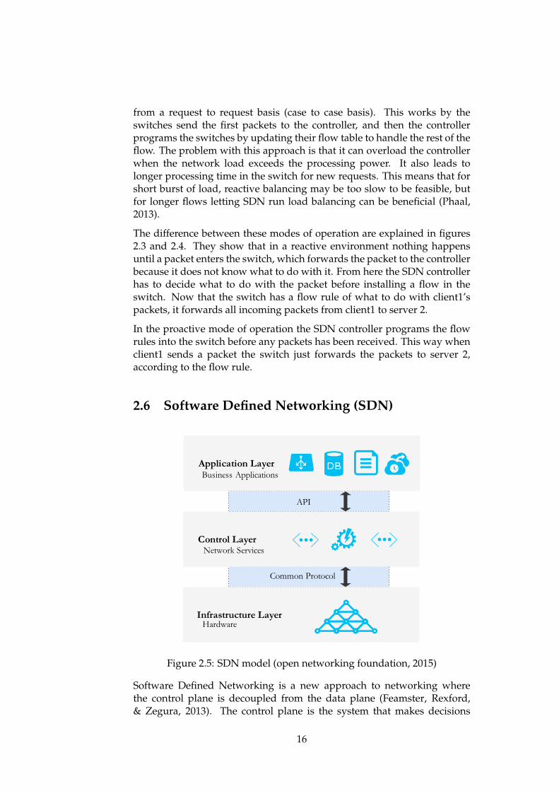
Reactive approach. . . . . . . . . . . . . . . . . . . . . . . . . 152.4 SDN Load Balancing in a OpenFlow network using a

Proactive approach. . . . . . . . . . . . . . . . . . . . . . . . . 152.5 SDN model (open networking foundation, 2015) . . . . . . . 162.6 OpenFlow enabled network vs traditional . . . . . . . . . . . 192.7 OpenFlow match fields for packets. . . . . . . . . . . . . . . . 202.8 The pipeline of OpenFlow (OpenFlow, 2013). (a) for the

whole pipeline. (b) for one table in the pipeline . . . . . . . . 212.9 Floodlight GUI at start page . . . . . . . . . . . . . . . . . . . 252.10 WireShark GUI with OpenFlow traffic packets captured . . . 272.11 VirtualBox GUI for Mininet instalation . . . . . . . . . . . . . 27

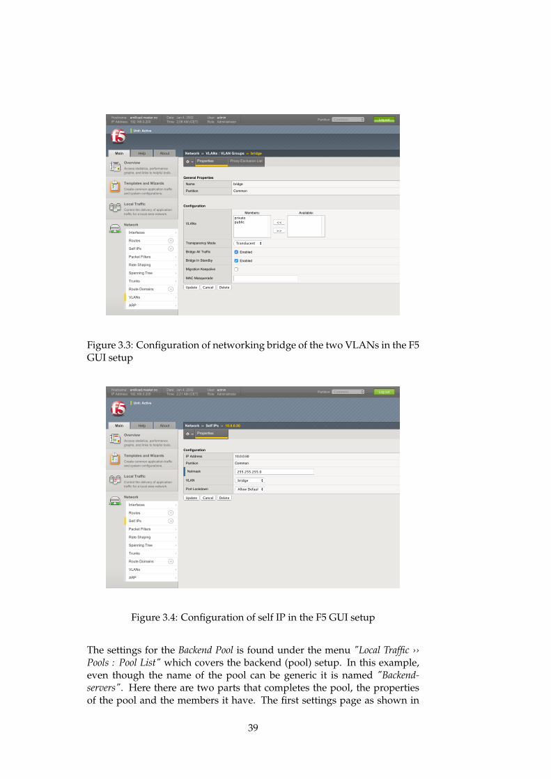
3.1 Testbed virtual setup . . . . . . . . . . . . . . . . . . . . . . . 343.2 Final hardware setup. . . . . . . . . . . . . . . . . . . . . . . . 373.3 Configuration of networking bridge of the two VLANs in the

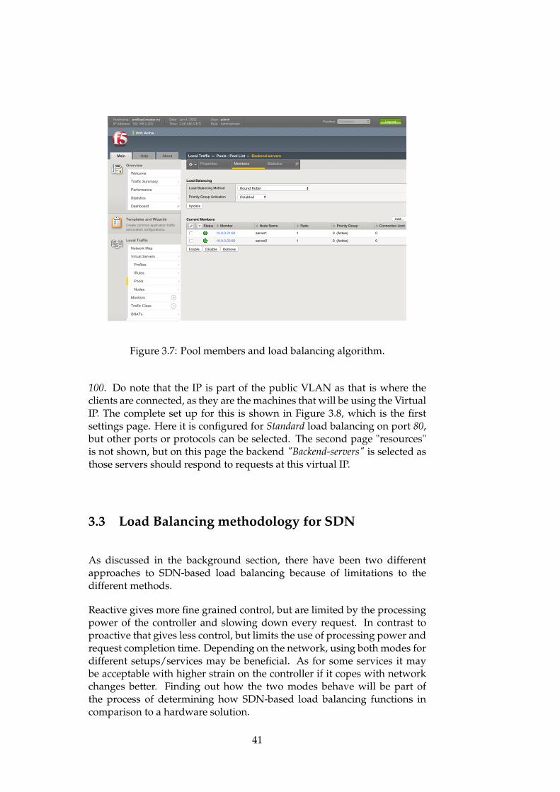
F5 GUI setup . . . . . . . . . . . . . . . . . . . . . . . . . . . . 393.4 Configuration of self IP in the F5 GUI setup . . . . . . . . . . 393.5 Inner workings of the F5 VLAN bridge and the Load

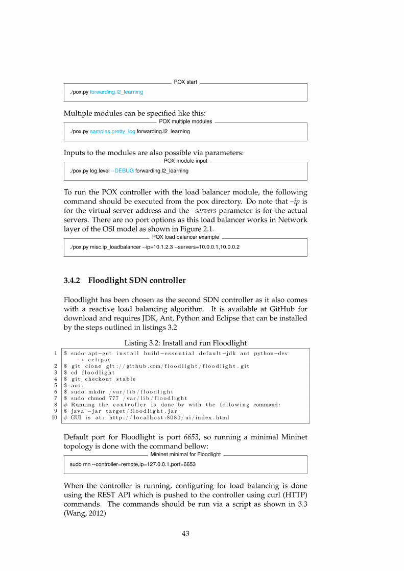
Balancing module. . . . . . . . . . . . . . . . . . . . . . . . . 403.6 Health monitoring properties for the pool. . . . . . . . . . . . 403.7 Pool members and load balancing algorithm. . . . . . . . . . 413.8 Virtual IP settings page. . . . . . . . . . . . . . . . . . . . . . 42

4.1 average latency comparison . . . . . . . . . . . . . . . . . . . 504.2 BIG-IP calculated saturation, after formula: 434.15x −

3223.52 . Showing RPS and CPU usage. . . . . . . . . . . . . 544.3 XTerm CLI starting HTTP server . . . . . . . . . . . . . . . . 554.4 SDN as a Load Balancing algorithm results . . . . . . . . . . 624.5 SDN as a Load Balancing algorithm results for large load . . 634.6 Proactive load balancing POX for few bytes in httperf.

Figure in base10, shows relativity between CPU usage ofswitch and RPS achieved. . . . . . . . . . . . . . . . . . . . . 66

4.7 Proactive and reactive performance diagram for httperf testsof few bytes . . . . . . . . . . . . . . . . . . . . . . . . . . . . 66

ix

4.8 Proactive and reactive performance diagram for httperf testsof 1MiB . . . . . . . . . . . . . . . . . . . . . . . . . . . . . . . 67

x

List of Tables

2.1 Specifications for the BIG-IP 1600 series . . . . . . . . . . . . 142.2 OpenFlow table example . . . . . . . . . . . . . . . . . . . . . 202.3 OpenFlow entries columns (OpenFlow, 2013). . . . . . . . . 20

3.1 Specifications for the virtual environment . . . . . . . . . . . 34

4.1 BIG-IP, results for few bytes (94) . . . . . . . . . . . . . . . . 534.2 BIG-IP, results for few bytes (94) CPU load . . . . . . . . . . 534.3 BIG-IP, results for 1 MiB . . . . . . . . . . . . . . . . . . . . . 554.4 POX Controller, results for few bytes (215) AB . . . . . . . . 574.5 POX Controller, results for few bytes (215) httperf . . . . . . 574.6 POX Controller, results(few bytes) httperf CPU percentage . 584.7 POX Controller, results for 1 MiB httperf . . . . . . . . . . . . 584.8 POX Controller, results for 1 MiB CPU usage httperf . . . . . 594.9 POX Controller, results for 2 MiB httperf . . . . . . . . . . . . 594.10 POX Controller, results for 2 MiB CPU usage httperf . . . . . 594.11 Floodlight Controller, results for few bytes (215) ab . . . . . 604.12 Floodlight Controller, results for few bytes (215) httperf . . . 604.13 Floodlight Controller, results(few bytes) httperf CPU per-

centage . . . . . . . . . . . . . . . . . . . . . . . . . . . . . . . 614.14 Floodlight Controller, results for 1MiB httperf . . . . . . . . . 614.15 Floodlight Controller, results for 1MiB CPU usage httperf . . 614.16 Proactive POX httperf test of 1 server at saturation point -

Request rate requested: 42 (req/s), B.1 . . . . . . . . . . . . . 644.17 Proactive POX httperf test of 2 servers at saturation point -

Request rate requested: 84 (42x2) (req/s), B.2 . . . . . . . . . 654.18 Proactive POX httperf test of servers at saturation point for

1 MiB . . . . . . . . . . . . . . . . . . . . . . . . . . . . . . . . 65

B.1 Proactive POX httperf test of 1 server-raw . . . . . . . . . . . 90B.2 Proactive POX httperf test of 2 servers-raw . . . . . . . . . . 91

xi

Preface

I would like to thank the following people for their support with my masterthesis:

• Desta Haileselassie Hagos for his support and help.

• Kyrre Begnum for providing the hardware load balancers.

• My friends, Arne and Samrin for helping me proof-read my thesis.

Finally, I would like to extend my gratitude to HiOA and UiO for fiverewarding years as a student, and for the opportunity to attend the networkand system administration programme.

xiii

Part I

Introduction

1

Chapter 1

Introduction

The introduction chapter begins with the motivation section where itdiscusses the problems of today’s networking, including how SDN can fixthose problems and introduce load balancing.

Next section covers the main problem statements this report takes on tosolve, before the thesis structure section defines the structure of the nextchapters. In the end there is the related work section, which introducesother related work with regards to the problem statement.

1.1 Motivation

After visiting the LISA conference of 2014, where Software DefinedNetworking (SDN) was one of the hot talks, it became clear that thistechnology is going to be the next big thing in networking. This is dueto the fact that SDN has promises in cost reduction, reduced complexity,better agility, more fine-grained security and simplification for networkadministrators. One of my criteria for choosing a master thesis was thatit had to be useful in regards to working in the sysadmin field aftergraduation. Getting to work with new and exciting technology as SDNfits that criterion.

What is happening now in the network industry is the same that happenedin the early stages of the computer industry. In the beginning, IBMwas computing with highly specialized hardware and software from onevendor. That all changed with the introduction of microprocessors, asthat introduced many different operating systems (McKeown, 2011) to runon them. These names as known by everyone today are systems likeWindows, Linux and Mac OS, and they can run a limitless possibility ofapplications.

The same thing is now happening with SDN, as it shows promise inincluding what was earlier a job for dedicated hardware into the networkitself. What SDN can achieve may redefine the norm of how networks

3

are built, as there already is a transition from traditional networking toSDN with the OpenFlow approach in particular. However, there are moreand more vendors expanding into SDN and providing their own SDNapproaches. In regards to the computer industry analogy, networks maynow run their own operation system on common hardware, instead ofbeing limited to a specific provider.

What is good about SDN is that it opens up a possibility for simplificationfor network administrators. By reducing the complexity for the paritiesinvolved, it provides an easier way into the understanding of networking.A way to look at SDN is that it provides an API for interaction with thenetwork. With such an API, applications may be available to the end usersin such an easy way as we are getting accommodated to by app stores onour phones (Johnson, 2012). A fully defined and provisioned SDN standardcan support apps to be installed with a push of a button. Configuration cantherefore be user specific as the SDN framework handles the complexity.For a business setting up a new service, the network may be reconfiguredwith ease instead of weeks of planning and box-to-box reconfiguring tosupport the new service.

In summary SDN will shape networking in the following ways (McKeown,2011):

1. It will empower the people involved with networking, as it can becustomized to fit local needs and eliminate unneeded features. It mayalso include desired features like load balancing.

2. It will increase the speed of innovation, as it provides innovationat the speed of which software is developed as in comparison tohardware development. For instance is rapid development availablein emulated environments like Mininet, with the ability to pushvirtualization developed code directly into the live physical networkswith no changes to the code.

3. It will diversify the supply chain, as more vendors and softwaresuppliers all can contribute to the same platform.

4. It will build a strong foundation for abstracting the networkingcontrol.

1.2 Problem Statement

Managing traffic in computer networks is very important and critical toensure a reliable service. This is because traffic often has a high fluctuation,which could result in overloaded devices and an unreliable service for theusers. Just like a webserver, a service can only have a limited amount ofsimultaneously users. If the limit has been reached, no additional userscan access the server. Load balancing is a solution that enables moreusers to access the service, but it is a challenge for network administrators.

4

Today’s solutions works, but it requires expensive dedicated hardware thatdoes not support fast changes in the network topology. BIG-IP is someof the working load balancers products that deliver load balancing viadedicated hardware. These load balancers come at a hefty price tag andmust be replaced when maximum capacity is reached. A Software DefinedNetworking (SDN) load balancer could replace the dedicated hardware,and instead run on commodity hardware.

The question that needs to be answered from a research point of view, is ifan SDN solution can match the dedicated hardware.

This thesis tries to address the problems as in the following scenario:

1. How to setup a load balancing algorithm in SDN in order to achieveperformance comparable to a physical load balancer.

(a) Study, setup and run a physical load balancer (BIG-IP-1600series).

(b) Compare a SDN-based load balancer to a hardware load bal-ancer in terms of scalability and performance.

1.3 Thesis Structure

• Chapter 1: This is the introduction chapter that introduces themotivation of this thesis and describes the problem statement.

• Chapter 2: The background chapter contains information about SDN,load balancing, tools and terms related to the understanding of thesesubjects.

• Chapter 3: This is the approach chapter. In this chapter, there is anexplanation of the methodology involved when tackling the problemstatement. In simpler words: It is a guideline for how to attempt tosolve the what.

• Chapter 4: This chapter contains the actual outcome of the methodsapplied from the approach, and the analysis of the presenteddata.

• Chapter 5: This chapter is a discussion of the results in the previouschapter, as it looks back and concludes the thesis. For Future Work ittries to give ways to continue the research in the same field as well asaddressing the research questions from the problem statement.

• Appendix: Finally, the appendix chapter includes significant docu-ments related to the thesis.

5

1.4 Related Work

SDN is a hot topic for research these days; meaning that there are manypublished papers about different SDN related investigation. Some of thosethat are related to the problem statement is discussed next.

1.4.1 OpenFlow-Based Server Load Balancing Gone Wild

Richard Wang, Dana Butnariu, and Jennifer from the Rexford PrincetonUniversity (Richard Wang, 2011) have explored the possibility of runningload balancing in the SDN network. Their approach was based on creatingas few wildcard rules as possible to insert into their switches. Thatenabled them to load balance proactively without involving the controller.However, they must make wildcard rules for the whole IP range and thensplit the IP ranges across multiple servers. The drawback of this approachis that the traffic from the whole IP range is often not uniform. Theytherefore had to implement an updating algorithm that changed the sizesof the IP range slices over time, which struggles with sudden changes inincoming traffic.

1.4.2 OpenFlow Based Load Balancing

At the University of Washington have Hardeep Uppal and Dane Brandondone a proof of concept, showing that there is possible to set up loadbalancing in the SDN network (Uppal & Brandon, n.d.). Their notationsare that running one controller still produces a single point of failure andthat their particular early generation of OpenFlow switches were very slowon rewriting packet header information.

1.4.3 Aster*x: Load-Balancing as a Network Primitive

At the Stanford University in USA, have they explored the possibilityof building load balancing directly into a campus network (Handigol,Seetharaman, Flajslik, Johari, & McKeown, 2010). Their work focuseson reliving congested routes in their network, by diverting traffic acrossmultiple links. This is done via a network of SDN enabled switcheswith their own controller application, Aster*x. The controller applicationdetermines the current state of the network and the servers, in order tochoose the appropriate server and path to direct requests to. Using theNOX controller, they have demonstrated what appears to be a workingprototype in multiple videos, but they only show a application GUI and noactual code has been published. Their work is however very interesting asthey explore multiple problems that occurs when building load balancingdirectly into a typical campus network. The work of this research paperis built on the paper about Plug-And-Serve a similar solution presented

6

by some of the same authors in 2009 (Handigol, Seetharaman, Flajslik,McKeown, & Johari, 2009).

1.4.4 Load Balancing in a Campus Network using SoftwareDefined Networking

Over at the Arizona State University, Ashkan Ghaffarinejad (student) andViolet R. Syrotiuk (professor/teacher) are attempting to create a SDN loadbalancing setup to compete with their dedicated hardware (Ghaffarinejad& Syrotiuk, 2014). Their requirement is that the SDN solution shouldcope better with the variation in their Campus network than the existingsetup. Unfortunately as this proposed solution seems promising, itis not complete. Ashkan is at this time working on his thesis, andtheir publication offers no real value until the full dissertation has beencompleted and published.

7

Chapter 2

Background

This chapter is a study in literature with regards to what is the necessaryinformation to know in order to understand the main part of this thesis.The covered topics will include the network model, load balancing, anexplanation of SDNs and information about useful tools.

2.1 The OSI model

The OSI model is a model of the layers that are in play in what is commonlyknow as the Internet-as-a-Service terminology. In Figure 2.1 the OSI modelis shown with information about what is contained in the different levels.Some of the levels that this thesis will depend upon will be described inmore detail.

2.1.1 Layer 1

Layer 1 is the physical layer of the OSI model, which consists of cablesand hubs. It does not, however, have to be an actual hub, but the device(switch/router) must have the capabilities of a hub included.

2.1.2 Layer 2

Layer 2 is the data link layer. It is responsible for multiple key tasks, butfor the purpose of this thesis it is important to understand that in this layer,data intended for a specific MAC address is only forwarded to that uniqueMAC address. The protocol most used here is Address Resolution Protocol(ARP).

9

Figure 2.1: OSI-model (Zito, 2013)

2.1.3 Layer 3

As layer 2 was responsible for data to the correct MAC address, layer3 is responsible for packet forwarding and routing through connectedrouters. This means that it depends on layer 2 working correctly. Commonprotocols at this layer are: IPv4/6 and ICMP.

2.1.4 Layer 4

Layer 4 provides end-to-end communication over multiple instances oflayer 1-3 networks. TCP is the most used protocol at this layer.

2.1.5 Layer 7

Layer 7 contains all user application communication, like HTTP and SMTP(email).

2.2 Traditional Networks

Today’s network devices are running a very specific set of hardware andsoftware. From providers like Cisco that packages both the hardware andsoftware into one single package. These devices are typically configuredone by one, because every device is in their own closed environment.

10

This means every device contains their own configuration and flows. Thismakes configuration complex and it is therefore hard to achieve a goodnetwork. This also means that when there are changes to the network,upgrading the devices to accommodate the increasing load is expensive.This approach has typically been in conflict with business requirements.That is it being to static, as it does not allow any interaction with the upperlayers of the OSI model. It also makes the networks very complex, meaningthat to upgrade a system with a new application, may involve rebuildingparts of the data center to accommodate the innovation (Morin, 2014). Themain point to take is that changing the traditional network structure is timeconsuming, so that when the change is in place the business decision tochange the network may be out-dated.

2.2.1 Networking devices

There are many different types of networking devices, some are simplewith little logic while others are complex devices with capabilities forthorough decision making. There is also mixes of them, but in this sectiononly the three most related to network routing are shown.

2.2.2 Hub

A network hub is often called a repeater and does not manage any of thetraffic. This means that for any packet coming through, it sends it out onevery other port, except for the port it originated from (Pacchiano, 2006). Ahub works only in the Layer 1 of the OSI model, so it’s repeating functioncause packet collisions which affect the network capacity (ContemporaryControl Systems, 2002).

2.2.3 Switch

A network switch is a upgrade of a network hub. It sill has to have thenetwork layer level 1, but it is created virtually in the switch. In contrastto the hub a switch only sends out a packet on one port, the correct one.There are two types of switches, unmanaged and managed switches. Thelatter supports configuration as the unmanaged is plug and play (CISCO,2015). In this thesis a switch will be referred to as a managed switch. Toonly send out packets on the correct port, a switch keeps a record of theMAC addresses of all the devices it is directly connected to.

2.2.4 Router

A router’s job is different from a switch. As the router is typically used toconnect at least two networks like Local Area Networks (LANs) or Wide

11

Area Networks (WANs). A router is placed in the network as gateways,which is where two networks meet. Using packet header informationand forwarding tables, a router can determine the best path to forward apacket (Pacchiano, 2006). Compared to a unmanaged switch, all routers areconfigurable in the sense that they use protocols like IMCP to communicatewith other routers in order to figure out the best route between two hosts(Pacchiano, 2006).

2.3 Load balancer

The job of a load balancer is to distribute workloads across multiple com-puting resources. This is for optimizing the resource usage, maximizingthroughput and lowering the response time to avoid overloading any sin-gle resource. Load balancers can be implemented in software or hardwareoften depending on what type of load they are distributing. Software loadbalancers are more cost efficient than hardware balancers, as they do notrequire specialized hardware.

A load balancer works by selecting a resource from a list of all availableresources. When it receives a request it then forwards the request to theresource it chose. It may have additional functions, like maintaining theresource list by testing if the resource is up, or if the resource is at anacceptable load level before forwarding any requests to it. This is oftena desired feature so that requests will be responded to by an availableresource.

There are multiple methods of operations a load balancer can function.For instance the selection of the resources can be randomly chosen froma list, but that may not be the most efficient method. Another mode isRound Robin where it starts at the top of the resource list, and for eachrequests it selects the next one until it is at the end where it jumps backto the beginning to repeat the procedure. Other modes exist, for instancethe least-connections, where it selects the resource with the least activeconnections.

In Figure 2.2 there is an example of how an layer 7 load balancer works.Any given client is matched to a working webserver decided by the loadbalancer.

2.4 Hardware load balancing

A hardware load-balancing device (HLD), also known as a layer 4-7, isa physical unit that forwards requests to individual servers in a network(Rouse, 2007). Which server it forwards to are determined by factorssuch as server CPU usage, the number of connections or the serversperformance. The benefit of using a HDL device is that it minimizes the

12

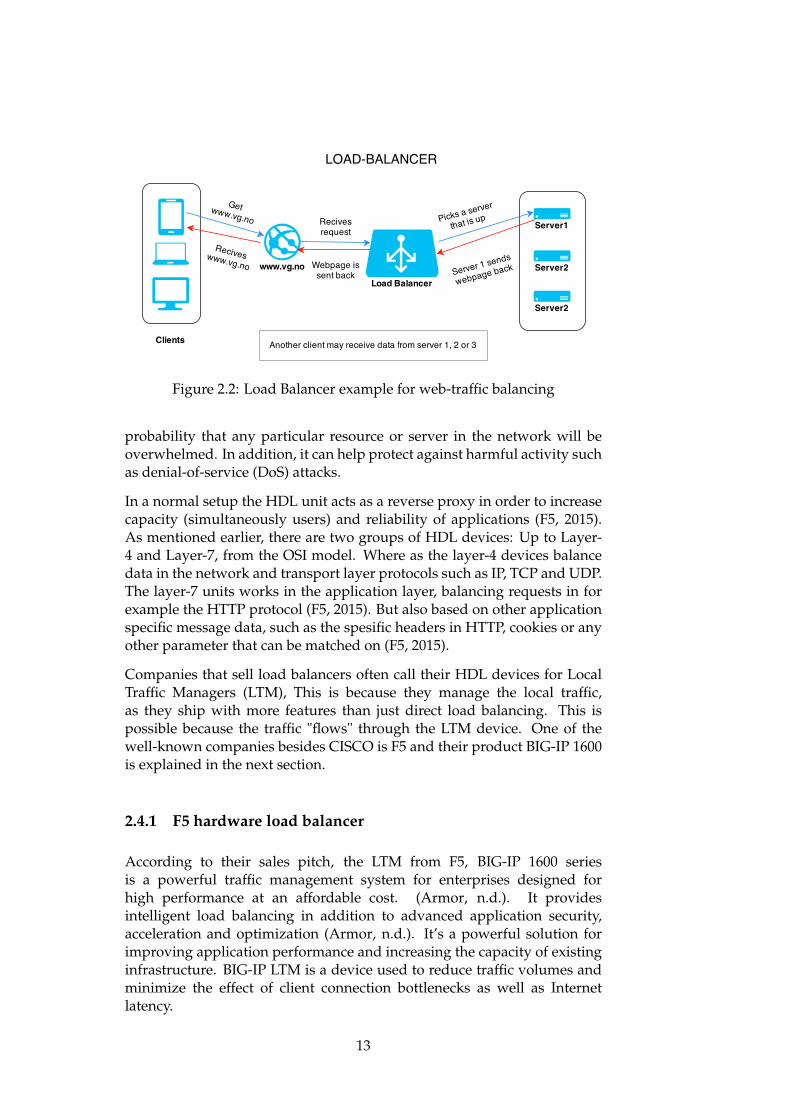
Figure 2.2: Load Balancer example for web-traffic balancing

probability that any particular resource or server in the network will beoverwhelmed. In addition, it can help protect against harmful activity suchas denial-of-service (DoS) attacks.

In a normal setup the HDL unit acts as a reverse proxy in order to increasecapacity (simultaneously users) and reliability of applications (F5, 2015).As mentioned earlier, there are two groups of HDL devices: Up to Layer-4 and Layer-7, from the OSI model. Where as the layer-4 devices balancedata in the network and transport layer protocols such as IP, TCP and UDP.The layer-7 units works in the application layer, balancing requests in forexample the HTTP protocol (F5, 2015). But also based on other applicationspecific message data, such as the spesific headers in HTTP, cookies or anyother parameter that can be matched on (F5, 2015).

Companies that sell load balancers often call their HDL devices for LocalTraffic Managers (LTM), This is because they manage the local traffic,as they ship with more features than just direct load balancing. This ispossible because the traffic "flows" through the LTM device. One of thewell-known companies besides CISCO is F5 and their product BIG-IP 1600is explained in the next section.

2.4.1 F5 hardware load balancer

According to their sales pitch, the LTM from F5, BIG-IP 1600 seriesis a powerful traffic management system for enterprises designed forhigh performance at an affordable cost. (Armor, n.d.). It providesintelligent load balancing in addition to advanced application security,acceleration and optimization (Armor, n.d.). It’s a powerful solution forimproving application performance and increasing the capacity of existinginfrastructure. BIG-IP LTM is a device used to reduce traffic volumes andminimize the effect of client connection bottlenecks as well as Internetlatency.

13

The BIG-IP 1600 series security feature is described as a firewall thatblock attacks while still serving legitimate users. It provides network andprotocol level security for filtering application attacks. Placing the BIG-IPLTM is recommended at a critical gateway to the most valuable resourcesin the network (Armor, n.d.). Another selling point for the BIG-IP 1600series is that it removes single points of failure by dynamic and static loadbalancing methods. Some of the available balancing methods are dynamicratio, least connections, observed load balancing and round robin.

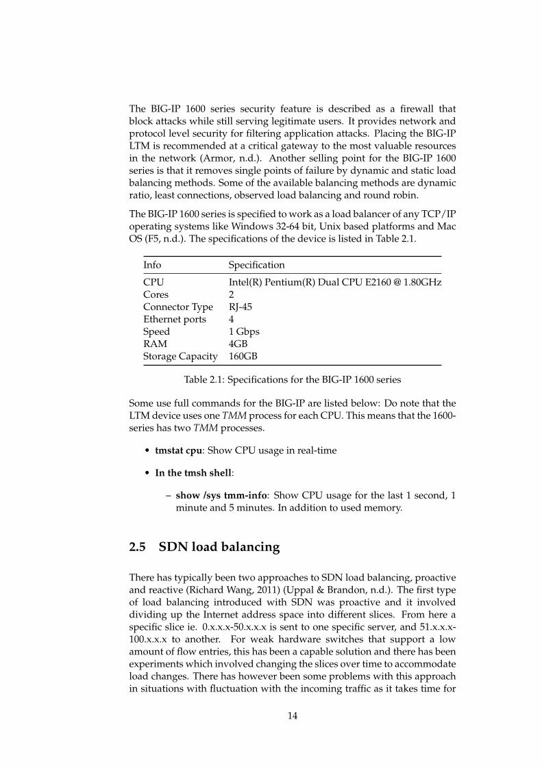
The BIG-IP 1600 series is specified to work as a load balancer of any TCP/IPoperating systems like Windows 32-64 bit, Unix based platforms and MacOS (F5, n.d.). The specifications of the device is listed in Table 2.1.

Info Specification

CPU Intel(R) Pentium(R) Dual CPU E2160 @ 1.80GHzCores 2Connector Type RJ-45Ethernet ports 4Speed 1 GbpsRAM 4GBStorage Capacity 160GB

Table 2.1: Specifications for the BIG-IP 1600 series

Some use full commands for the BIG-IP are listed below: Do note that theLTM device uses one TMM process for each CPU. This means that the 1600-series has two TMM processes.

• tmstat cpu: Show CPU usage in real-time

• In the tmsh shell:

– show /sys tmm-info: Show CPU usage for the last 1 second, 1minute and 5 minutes. In addition to used memory.

2.5 SDN load balancing

There has typically been two approaches to SDN load balancing, proactiveand reactive (Richard Wang, 2011) (Uppal & Brandon, n.d.). The first typeof load balancing introduced with SDN was proactive and it involveddividing up the Internet address space into different slices. From here aspecific slice ie. 0.x.x.x-50.x.x.x is sent to one specific server, and 51.x.x.x-100.x.x.x to another. For weak hardware switches that support a lowamount of flow entries, this has been a capable solution and there has beenexperiments which involved changing the slices over time to accommodateload changes. There has however been some problems with this approachin situations with fluctuation with the incoming traffic as it takes time for

14

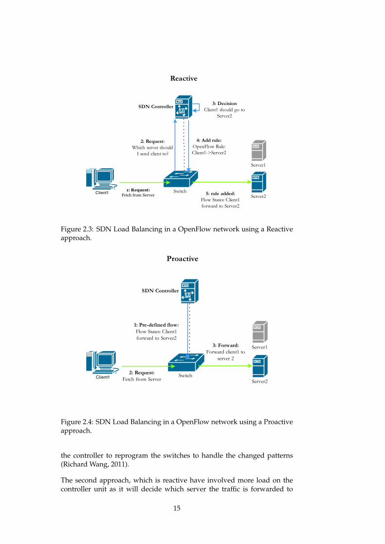
Figure 2.3: SDN Load Balancing in a OpenFlow network using a Reactiveapproach.

Figure 2.4: SDN Load Balancing in a OpenFlow network using a Proactiveapproach.

the controller to reprogram the switches to handle the changed patterns(Richard Wang, 2011).

The second approach, which is reactive have involved more load on thecontroller unit as it will decide which server the traffic is forwarded to

15

from a request to request basis (case to case basis). This works by theswitches send the first packets to the controller, and then the controllerprograms the switches by updating their flow table to handle the rest of theflow. The problem with this approach is that it can overload the controllerwhen the network load exceeds the processing power. It also leads tolonger processing time in the switch for new requests. This means that forshort burst of load, reactive balancing may be too slow to be feasible, butfor longer flows letting SDN run load balancing can be beneficial (Phaal,2013).

The difference between these modes of operation are explained in figures2.3 and 2.4. They show that in a reactive environment nothing happensuntil a packet enters the switch, which forwards the packet to the controllerbecause it does not know what to do with it. From here the SDN controllerhas to decide what to do with the packet before installing a flow in theswitch. Now that the switch has a flow rule of what to do with client1’spackets, it forwards all incoming packets from client1 to server 2.

In the proactive mode of operation the SDN controller programs the flowrules into the switch before any packets has been received. This way whenclient1 sends a packet the switch just forwards the packets to server 2,according to the flow rule.

2.6 Software Defined Networking (SDN)

Figure 2.5: SDN model (open networking foundation, 2015)

Software Defined Networking is a new approach to networking wherethe control plane is decoupled from the data plane (Feamster, Rexford,& Zegura, 2013). The control plane is the system that makes decisions

16

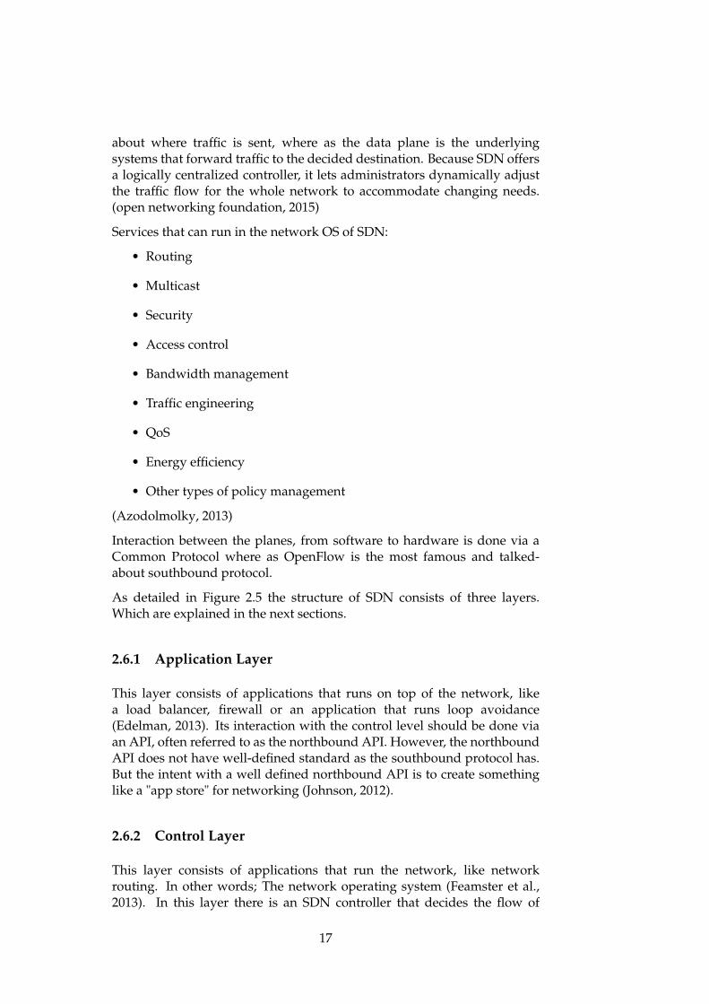
about where traffic is sent, where as the data plane is the underlyingsystems that forward traffic to the decided destination. Because SDN offersa logically centralized controller, it lets administrators dynamically adjustthe traffic flow for the whole network to accommodate changing needs.(open networking foundation, 2015)

Services that can run in the network OS of SDN:

• Routing

• Multicast

• Security

• Access control

• Bandwidth management

• Traffic engineering

• QoS

• Energy efficiency

• Other types of policy management

(Azodolmolky, 2013)

Interaction between the planes, from software to hardware is done via aCommon Protocol where as OpenFlow is the most famous and talked-about southbound protocol.

As detailed in Figure 2.5 the structure of SDN consists of three layers.Which are explained in the next sections.

2.6.1 Application Layer

This layer consists of applications that runs on top of the network, likea load balancer, firewall or an application that runs loop avoidance(Edelman, 2013). Its interaction with the control level should be done viaan API, often referred to as the northbound API. However, the northboundAPI does not have well-defined standard as the southbound protocol has.But the intent with a well defined northbound API is to create somethinglike a "app store" for networking (Johnson, 2012).

2.6.2 Control Layer

This layer consists of applications that run the network, like networkrouting. In other words; The network operating system (Feamster et al.,2013). In this layer there is an SDN controller that decides the flow of

17

packets in the network. Many controllers exist, but they all follow thesame principle. The interaction with hardware is often refereed to as thesouthbound protocol, because it is the layer below. This makes the controllayer the glue that binds the planes together. The most widespread andtalked about southbound protocol is OpenFlow. There are vendor specificalternatives to OpenFlow, but they all are common protocols for interactionbetween the layers.

2.6.3 Infrastructure Layer

This layer consists of the actual physical/virtual hardware, like a switch.This hardware is not specialised for the tasks the above layers demands,it can be just a simple switch that supports SDN and packet forwarding.Everything logical has already been taken care of by the controller, so thedevices in this layer only follows orders (Feamster et al., 2013).

2.7 OpenFlow

OpenFlow was the first standard interface between the control and dataplan layers in networking. It aims to ease the work for the networkadministrators by implementing a SDN open common protocol (Feamsteret al., 2013).

For a scenario where a data center has thousands or even hundredsof servers connected to the network, managing separation like VLANs(virtual LAN) on every closed box in the network would be an enormoustask. Adding that many networks dynamically change, it leads to problemsfor the network administrators. What SDN can do by using the OpenFlowstandard is to centralize this task to a logical controlling unit, where it iseasy to program VLAN like functionality. Do note that OpenFlow in it selfdoes not provide the standard VLANs, but rather a Layer3 policy of whocan talk to whom (Cole, 2013), (Feamster et al., 2013).

A visualisation of how OpenFlow differs from a traditional network setupcan be seen in Figure 2.6. Here it shows that the traditional networkenvironment has the control and data plane contained in each unit, whereas in the OpenFlow enabled environment it is separated.

OpenFlow is just a protocol, namely a specification on how the communi-cation between the control and data plane is handled. It runs over TCP andhas support for SSL to secure the communication between the switch andcontroller.

18

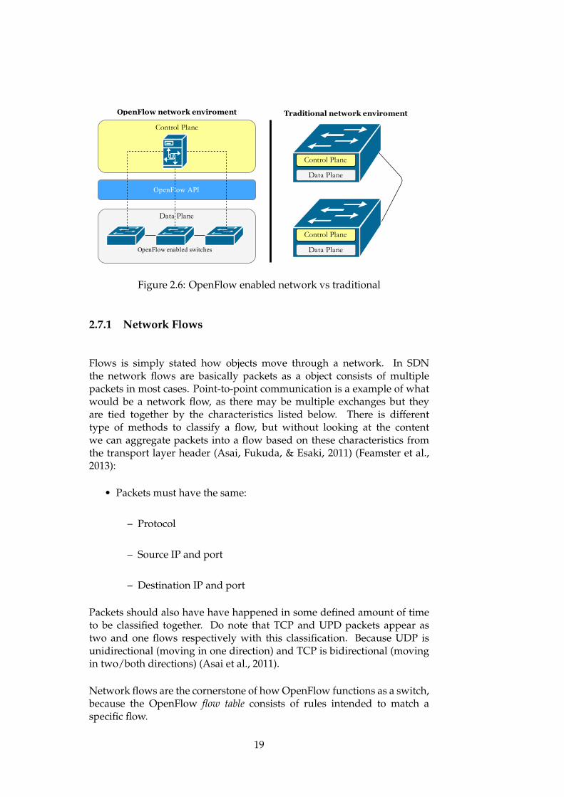
Figure 2.6: OpenFlow enabled network vs traditional

2.7.1 Network Flows

Flows is simply stated how objects move through a network. In SDNthe network flows are basically packets as a object consists of multiplepackets in most cases. Point-to-point communication is a example of whatwould be a network flow, as there may be multiple exchanges but theyare tied together by the characteristics listed below. There is differenttype of methods to classify a flow, but without looking at the contentwe can aggregate packets into a flow based on these characteristics fromthe transport layer header (Asai, Fukuda, & Esaki, 2011) (Feamster et al.,2013):

• Packets must have the same:

– Protocol

– Source IP and port

– Destination IP and port

Packets should also have have happened in some defined amount of timeto be classified together. Do note that TCP and UPD packets appear astwo and one flows respectively with this classification. Because UDP isunidirectional (moving in one direction) and TCP is bidirectional (movingin two/both directions) (Asai et al., 2011).

Network flows are the cornerstone of how OpenFlow functions as a switch,because the OpenFlow flow table consists of rules intended to match aspecific flow.

19

2.7.2 OpenFlow Flow Table

There may be multiple Flow tables in a switch, like firewall, QoS, NATand Forwarding. But this section covers what is in one table. In thefollowing Table 2.2 is an very short example rule set for a Flow table: Donote that this is only a simplified example and that the actual table is morecomplex.

Table 2.2: OpenFlow table example# Header Fields Actions Priorities1 if in_port = 1 output to port 2 1002 if IP = 10.1.2.3 rewrite to 84.4.3.2, output port 6 200

The first rule in Table 2.2 states that if a packet arrives into the switch onport 1 it should be sent out on port 2. But if a packet arrives at port 1 and ithas source IP 10.1.2.3 there is suddenly two rule matches for that particularpacket. To then decide what will happen to the packet the column prioritieswill be used. In this case as the second rule has priority of 200 which isgreater than 100 for the first rule. The switch would then use rule 2 andrewrite the IP to 84.4.3.2 and output it on port 6.

IP Dst IP Protocol

TCP sport

TCP dport

Switch Port

MAC src

MAC dst

Eth type

VLAN ID

IP Src

Supported OpenFlow packet headers filters

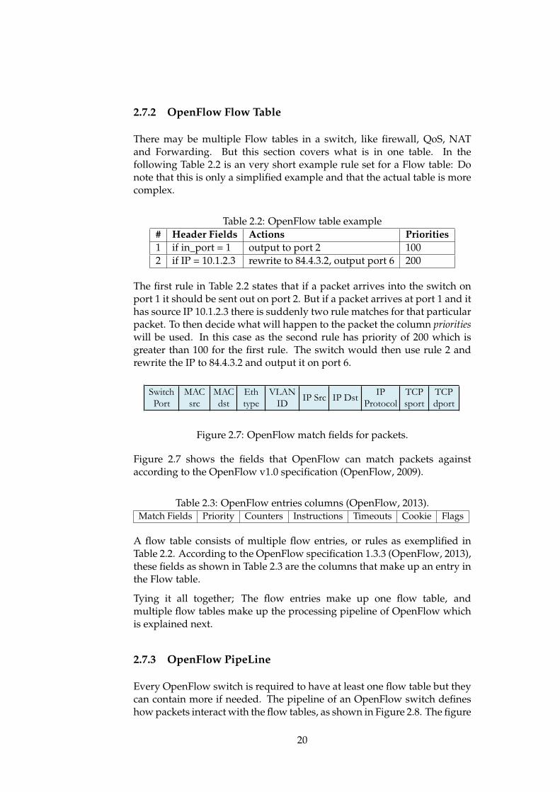
Figure 2.7: OpenFlow match fields for packets.

Figure 2.7 shows the fields that OpenFlow can match packets againstaccording to the OpenFlow v1.0 specification (OpenFlow, 2009).

Table 2.3: OpenFlow entries columns (OpenFlow, 2013).Match Fields Priority Counters Instructions Timeouts Cookie Flags

A flow table consists of multiple flow entries, or rules as exemplified inTable 2.2. According to the OpenFlow specification 1.3.3 (OpenFlow, 2013),these fields as shown in Table 2.3 are the columns that make up an entry inthe Flow table.

Tying it all together; The flow entries make up one flow table, andmultiple flow tables make up the processing pipeline of OpenFlow whichis explained next.

2.7.3 OpenFlow PipeLine

Every OpenFlow switch is required to have at least one flow table but theycan contain more if needed. The pipeline of an OpenFlow switch defineshow packets interact with the flow tables, as shown in Figure 2.8. The figure

20

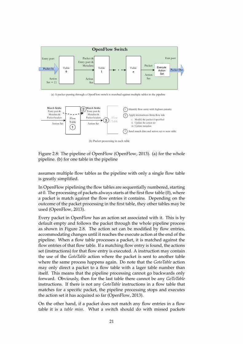
Figure 2.8: The pipeline of OpenFlow (OpenFlow, 2013). (a) for the wholepipeline. (b) for one table in the pipeline

assumes multiple flow tables as the pipeline with only a single flow tableis greatly simplified.

In OpenFlow pipelining the flow tables are sequentially numbered, startingat 0. The processing of packets always starts at the first flow table (0), wherea packet is match against the flow entries it contains. Depending on theoutcome of the packet processing in the first table, they other tables may beused (OpenFlow, 2013).

Every packet in OpenFlow has an action set associated with it. This is bydefault empty and follows the packet through the whole pipeline processas shown in Figure 2.8. The action set can be modified by flow entries,accommodating changes until it reaches the execute action at the end of thepipeline. When a flow table processes a packet, it is matched against theflow entries of that flow table. If a matching flow entry is found, the actionsset (instructions) for that flow entry is executed. A instruction may containthe use of the GotoTable action where the packet is sent to another tablewhere the same process happens again. Do note that the GotoTable actionmay only direct a packet to a flow table with a lager table number thanitself. This means that the pipeline processing cannot go backwards onlyforward. Obviously, then for the last table there cannot be any GoToTableinstructions. If there is not any GotoTable instructions in a flow table thatmatches for a specific packet, the pipeline processing stops and executesthe action set it has acquired so far (OpenFlow, 2013).

On the other hand, if a packet does not match any flow entries in a flowtable it is a table miss. What a switch should do with missed packets

21

depends on the configuration in the form of a table miss flow entry. Theseoptions for the switch are to drop the packet, pass them to another table orsend them to the controller (OpenFlow, 2013).

2.7.4 OpenFlow versions

The first version of OpenFlow was released in 2009. It would then be almosttwo years before version 1.1 came out and added support for Multi-tablepipeline processing, MPLS and QinQ. Followed by the release of version 1.210 months later, it added support for IPv6 and additional extensibility. In2012 version 1.3 was released adding support of QOS alongside with otherfeatures, followed by the release of 1.4 in 2013 (Oliver, 2014). Version 1.4introduced support for decision hierarchy and multiple controllers alongwith other features. At the end of last year, 2014, the specifications for 1.5was released and approved by the open network foundation (ONF) board,but has not yet been approved by all parties and finalized.

Although new releases of OpenFlow come out, there is a lack of vendorsincluding support for the newest versions of OpenFlow in their productsbefore the marked demands it (Oliver, 2014).

2.8 OpenFlow switch

Because a switch that runs the OpenFlow protocol has it’s decision makingtaking away from it, it differs from a normal switch. In a way thissimplifies the switches as they don’t think for them self, but rather havetheir decisions taken by a central controller. (Limoncelli, 2012). EveryOpenFlow switch has to have the support of at least one flow table, whichis changed by the controller via add, delete or update. A flow table containsflows; namely a rule for a specific packet occurrence. These flow rulesspecify what to do with a packet if it matches the criteria of the flowrule.

These flows can be installed in the switch proactively by installing thembefore any packet comes in, or reactively where as when the switch receivesa packet without a matching flow it asks the controller for what to do withthe packet.

Not all switches support this protocol, but it is getting more common thatthe switch vendors are including OpenFlow support in their products. Be-cause including support has often been a simple firmware upgrade.

The biggest constraint with OpenFlow switches has been in the lower-endsection as they come with less TCAM space. TCAM is a special lookupRAM for switches that can take three different inputs: 0, 1 and X (Salisbury,2012). It is used to store flow rules, for fast lookups. But as OpenFlow

22

support very fine grained control, there may be many rules required andrunning out of TCAM space to store the rules is a problem.

2.9 OpenFlow controllers

There is a wide selection of OpenFlow controllers, like NOX, POX, Trema,Beacon, OpenDaylight and Floodlight (Pronschinske, 2013). However inthis thesis the controllers POX and Floodlight has been chosen.

2.9.1 POX

POX is a framework for interacting with OpenFlow switches written inPython (NOXRepo.org, 2015). It is a sibling of the original SDN controllerNOX (written in c++), where their main difference is their scriptinglanguage. Due to POX being written in Python it is the recommendedcontroller to start with according to Murphy McCauley, the maintainer ofNOX/POX (Chua, 2012). This also meas that it can be run under mostplatforms such as Linux/Unix and Windows. A POX installation includesdifferent modules that resembles different type of normal switch behavior,in addition to other routing modules it supports custom modules. Some ofthe POX components provide core functionality, some are for convenientfeatures and some are just examples. In the list below some of thesecomponents are listed (M. McCauley & Al-Shabibi, 2014):

• forwarding.l2_learning: This POX component enables a OpenFlowswitch to become a layer 2 (L2) learning switch. This component triesto make flow rules are exact as possible. I.E, it tries to match on asmany fields as possible. This means that different TCP connectionswill results in different flow rules.

• forwarding.l3_learning: This component should be a router as it islabeled as an L3 device, but it is not quite a router. It is a L3-learning-switchy-thing (M. McCauley & Al-Shabibi, 2014), and used to test ARPrequests and responses.

• forwarding.l2_multi: This component is sort of a learning switch,but is has an additional feature. Normal learning switches learntheir connections on a switch-by switch basis, making decisionsonly about what they are directly connected to. l2_multi uses theopenflow.discovery and learns the topology of the entire network. Thismeans that when one switch learns where a a MAC address is, theyall do and can therefore make decisions based on that.

• openflow.discovery: This component uses the Link Layer DiscoveryProtocol to discover the network topology.

23

• openflow.spanning_tree: This component uses the information fromthe openflow.discovery component to provide a loop free network. Itworks sort of a Spanning Tree protocol, but it is not the exact samething.

• openflow.keepalive: Because some OpenFlow switches assumes thatan idle connection to the controller is the same as loss of connectivityand will disconnect after some time. This component ensures thatthe connection is refreshed by periodically sending ECHO requests,so they switches does not disconnect.

• proto.dhcpd This component acts as a DHCP server, leasing outDHCP addresses to clients.

• misc.gephi_topo: This component provides a visualization ofswitches, links, and detected hosts.

2.9.2 Floodlight

Floodlight is an OpenFlow controller written in Java that requires fewdependencies, enabling it to be run on a variety of platforms. Releasedwith the Apache license, Floodlight can be used for almost any purpose(Floodlight, 2015).

Similar to POX, it is also module based, making its functionality easyto extend. In addition, Floodlight delivers high performance, as it isthe core of a commercial product from Big Switch Networks. It comeswith support for many different virtual and physical OpenFlow enabledswitches. Interactions with the controller are issued using the REST API,which is an API that uses the HTTP protocol for easy interaction with thecontroller. (Floodlight, 2015).

As of version 1.0, support for OpenFlow protocol 1.0 and 1.3 are stably im-plemented, any versions of Floodlight before 1.0 only supports OpenFlow1.0. Other versions of OpenFlow only have experimental support in Flood-light (Floodlight, 2015).

Some Northbound API applications come bundled with Floodligh, theseare OpenStack Quantum, Virtual Switch, ACL (stateless FW) and CircuitPusher. But other applications can be written and loaded as modules.

Because Floodlight uses an HTTP based API it also has a GUI that isaccessible via a web browser as shown in Figure 2.9.

2.10 Testbeds

As OpenFlow enabled devices are not common hardware at the Universityof Oslo, working with SDN networking will require a virtual environment

24

Figure 2.9: Floodlight GUI at start page

for testing purposes.

2.10.1 Mininet

Mininet is a application that can create a network of virtual hosts, switches,controllers, and links on a single machine. Spawned switches supportOpenFlow for Software-Defined networking emulation and the virtualhosts run standard Linux software. As this closely emulates a physicalnetwork, it is ideal for research proposes. It relies on a Linux feature callednetwork namespaces, making kernels above version 2.2.26 a requirementfor Mininet to function. But this also means that it runs real code includingstandard network applications as well as the real Linux kernel and networkstack. As it supports arbitrary custom topologies, any custom network canbe emulated. To be able to setup a custom network, Mininet has a PythonAPI that allows the creation and testing of networks via a python script.(Team, 2015)

Mininet has been mostly used to demonstrate proof of concept’s, instead ofperformance because there is a overhead when emulating data flows. Thisis because packets first need to be exchanged between the virtual switchesto emulate packet flows. Which results in the switch sending a Packet-Into the controller, where a kernel to user space context switch happens andinduces overhead. This slows down the control plane traffic the Mininet

25

testbed can emulate.

The advantages for using Mininet for research purposes as compared to afully deployed virtual network is that is uses less resources, boots up faster,scales better and that it is easy to install. That is why Mininet is going tobe used in this thesis as a testbed for running OpenFlow controller againstOpen vSwitches. vSwitch is referred to ovs in the Mininet cli, and is a opensource, production quality, multilayer virtual switch.

2.11 Benchmarking/assisting tools

2.11.1 Iperf

Iperf is a command line utility to measure bandwidth between hosts. Inorder to use it one of two hosts must be started as a server and the other asa client.Iperf works by setting up a TCP or UDP connection where it pushesas many packets between the client and server as it can, and measuring thebandwidth it achieved between them. (Iperf, 2014) Both software’s partsare bundled in the same repository package, and the mode of operation isselected at boot for either client or server.

2.11.2 Wireshark

Wireshark is a free and open-source application for packet analysis andnetwork troubleshooting. It is a cross-platform application, running onmost Unix like operating systems and Microsoft Windows (Wireshark,2015). It has support for dissecting most networking protocols, but someprotocols requires a dissector plugin for optimal usage. It will capturepackets that are unknown, but to decode specific information about theOpenFlow packets or to filter them correctly the openflow.lua plugin isneeded.

By providing the user with a GUI (Graphical User Interface), Wiresharkallows live view of the network traffic on the network card it is listening to.In this thesis Wireshark will be used to listen at the loopback interface, as allthe Mininet testbed traffic passes through that virtual network card.

2.11.3 Tcpdump

Tcpdump is very similar to Wireshark, as this tool also captures packetspassing an interface. There is, however, no GUI as it is a command linetool. It runs on most Linux systems and will be used on the individualvirtual hosts in Mininet to analyze network behavior.

26

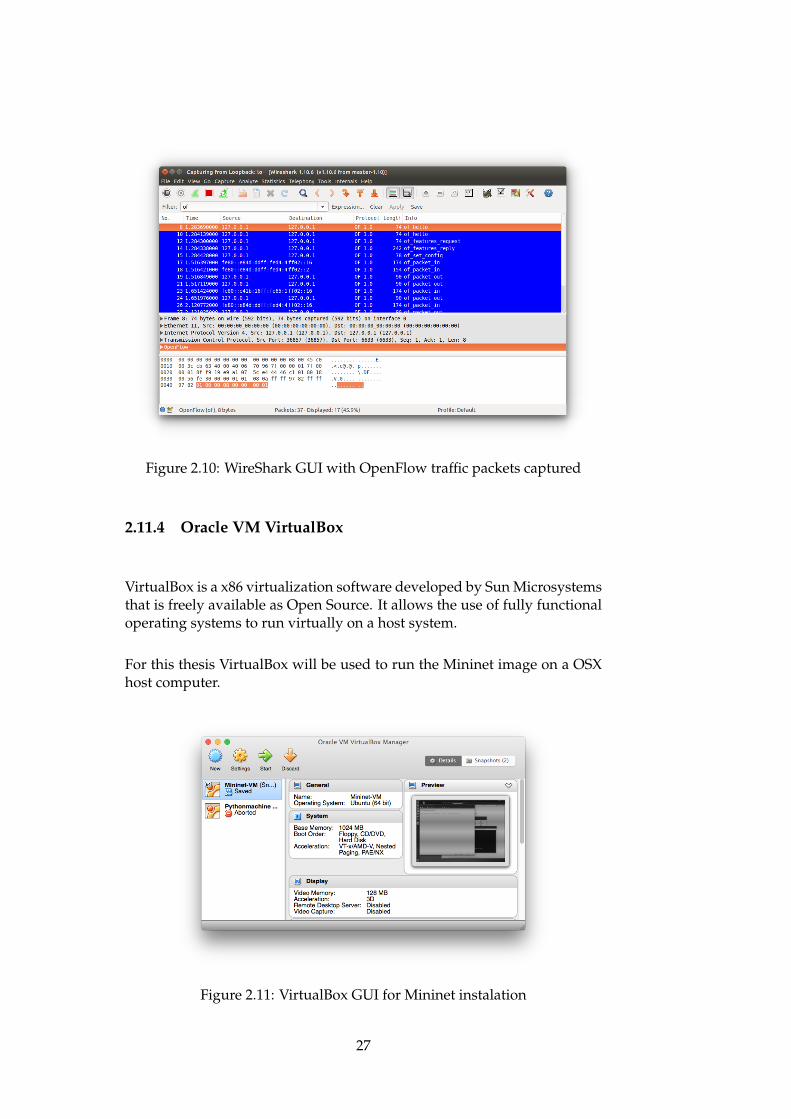
Figure 2.10: WireShark GUI with OpenFlow traffic packets captured

2.11.4 Oracle VM VirtualBox

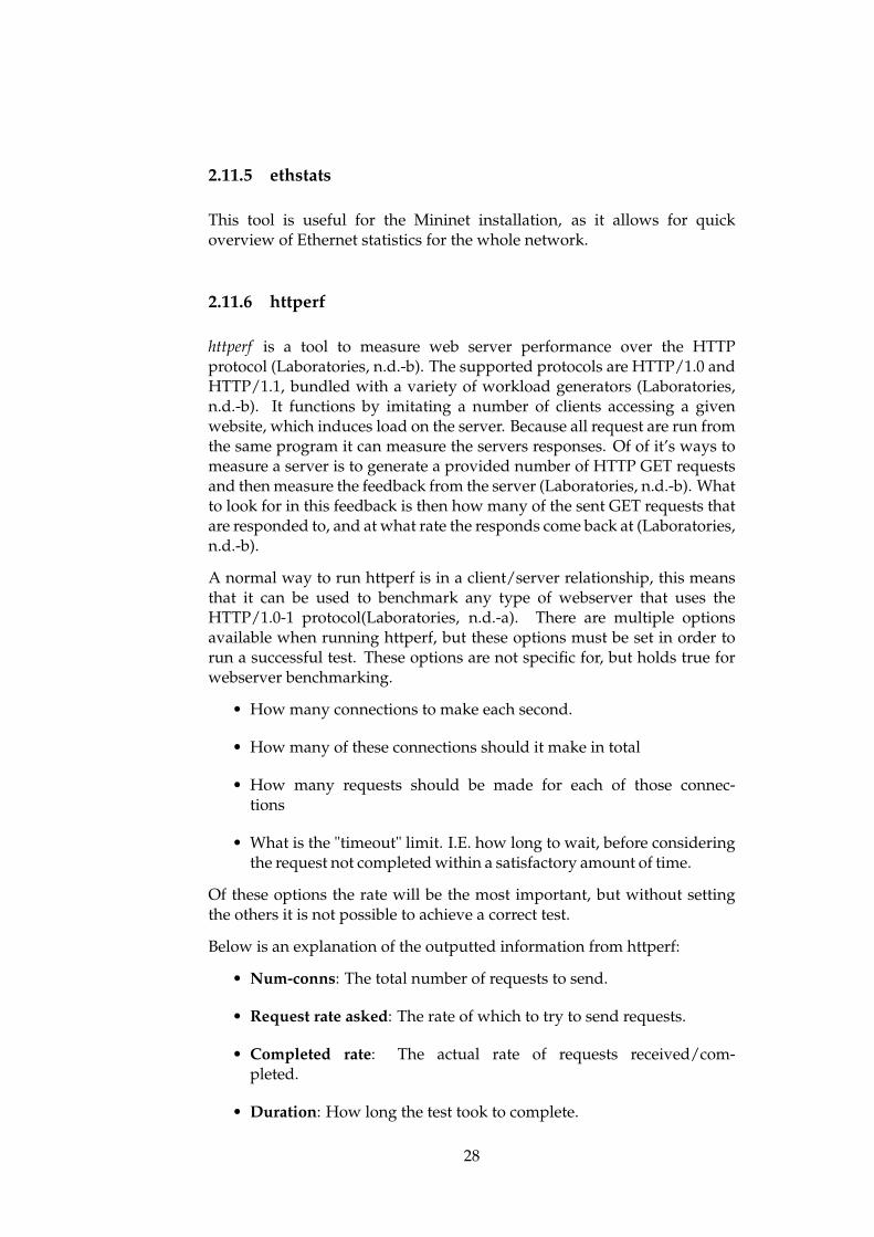
VirtualBox is a x86 virtualization software developed by Sun Microsystemsthat is freely available as Open Source. It allows the use of fully functionaloperating systems to run virtually on a host system.

For this thesis VirtualBox will be used to run the Mininet image on a OSXhost computer.

Figure 2.11: VirtualBox GUI for Mininet instalation

27

2.11.5 ethstats

This tool is useful for the Mininet installation, as it allows for quickoverview of Ethernet statistics for the whole network.

2.11.6 httperf

httperf is a tool to measure web server performance over the HTTPprotocol (Laboratories, n.d.-b). The supported protocols are HTTP/1.0 andHTTP/1.1, bundled with a variety of workload generators (Laboratories,n.d.-b). It functions by imitating a number of clients accessing a givenwebsite, which induces load on the server. Because all request are run fromthe same program it can measure the servers responses. Of of it’s ways tomeasure a server is to generate a provided number of HTTP GET requestsand then measure the feedback from the server (Laboratories, n.d.-b). Whatto look for in this feedback is then how many of the sent GET requests thatare responded to, and at what rate the responds come back at (Laboratories,n.d.-b).

A normal way to run httperf is in a client/server relationship, this meansthat it can be used to benchmark any type of webserver that uses theHTTP/1.0-1 protocol(Laboratories, n.d.-a). There are multiple optionsavailable when running httperf, but these options must be set in order torun a successful test. These options are not specific for, but holds true forwebserver benchmarking.

• How many connections to make each second.

• How many of these connections should it make in total

• How many requests should be made for each of those connec-tions

• What is the "timeout" limit. I.E. how long to wait, before consideringthe request not completed within a satisfactory amount of time.

Of these options the rate will be the most important, but without settingthe others it is not possible to achieve a correct test.

Below is an explanation of the outputted information from httperf:

• Num-conns: The total number of requests to send.

• Request rate asked: The rate of which to try to send requests.

• Completed rate: The actual rate of requests received/com-pleted.

• Duration: How long the test took to complete.

28

2.11.7 ApacheBench (ab) - Apache HTTP server benchmarkingtool

ab is another tool to measure web server performance over the HTTPprotocol.

The ab output and options are explained below:

• RPS: Requests Per Second, how many requests per secondachieved.

• Duration: How long the test took to complete.

• Kbytes/s: The transfer rate achieved in Kbytes/s.

• ms: Mean time per requests (ms), for all concurrent requests(individually)

• -c: How many concurrent requests to send.

• -n: The total number of requests to send.

29

Part II

The project

31

Chapter 3

Planning the project

This chapter is dedicated to the planning of the project, often referred toas the approach. It gives an overview of what to come, by introducingthe environments and methodology. In addition to this, it provides aninsight into how the experiments will be conducted. The main idea ofthis thesis is to evaluate how feasible an SDN-based load balancer is. Inorder to do so, it must be compared to an existing solution. A goodreference point would then be a hardware load balancer, tested against theSDN-based solution in terms of performance. But as there are multipleSDN controllers available, testing two different controller solutions toload balancing is beneficial in determining how viable SDN-based loadbalancing is. However, existing solutions may not bee fast enough, sothat developing the fastest possible scenario should give reference data fordetermining SDN-based load balancing feasibility.

3.1 Testbed design

In order to compare a result there is a need of at least two different inputparameters. In this case the inputs will come from different setups, but asthere is a lack of available OpenFlow enabled switches at the HiOA/UiOcampus for experiments, one of the setups must be virtualized. As for theother setup HiOA provides Jottacloud’s old F5 hardware load balancers,with corresponding server hardware.

The next sections will explore the different designs as we try to matchthe virtual environment to our hardware environment as closely aspossible.

3.1.1 Virtual environment with Mininet

For research purposes regarding SDN, Mininet is the obvious choice whenit comes to performance and ease of use. The provided image of Mininet

33

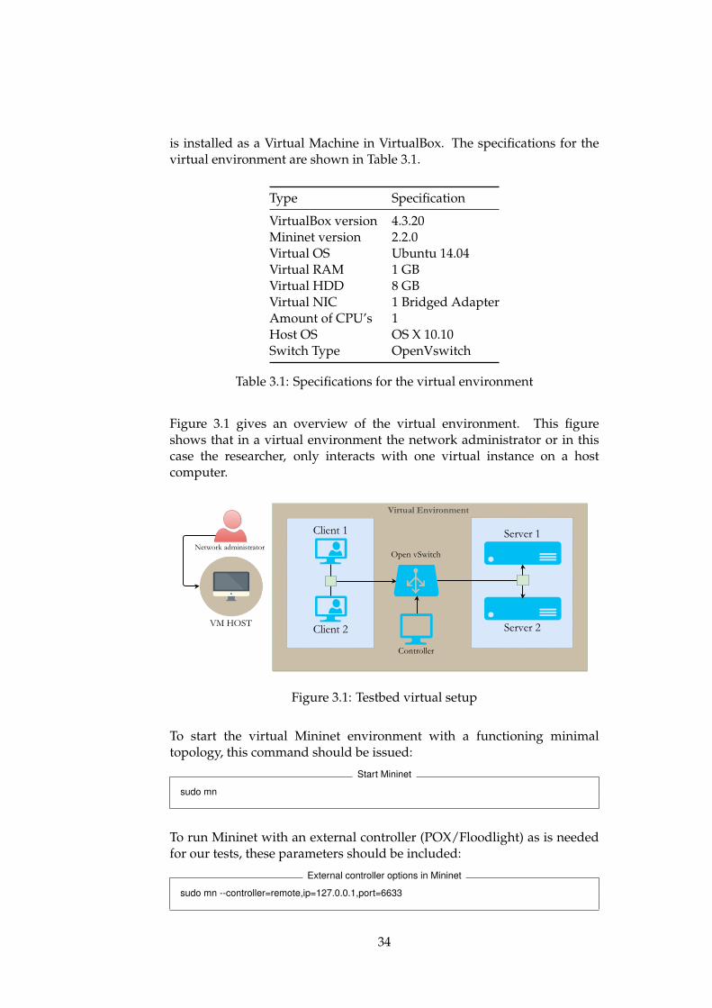
is installed as a Virtual Machine in VirtualBox. The specifications for thevirtual environment are shown in Table 3.1.

Type Specification

VirtualBox version 4.3.20Mininet version 2.2.0Virtual OS Ubuntu 14.04Virtual RAM 1 GBVirtual HDD 8 GBVirtual NIC 1 Bridged AdapterAmount of CPU’s 1Host OS OS X 10.10Switch Type OpenVswitch

Table 3.1: Specifications for the virtual environment

Figure 3.1 gives an overview of the virtual environment. This figureshows that in a virtual environment the network administrator or in thiscase the researcher, only interacts with one virtual instance on a hostcomputer.

Figure 3.1: Testbed virtual setup

To start the virtual Mininet environment with a functioning minimaltopology, this command should be issued:

Start Mininet

sudo mn

To run Mininet with an external controller (POX/Floodlight) as is neededfor our tests, these parameters should be included:

External controller options in Mininet

sudo mn --controller=remote,ip=127.0.0.1,port=6633

34

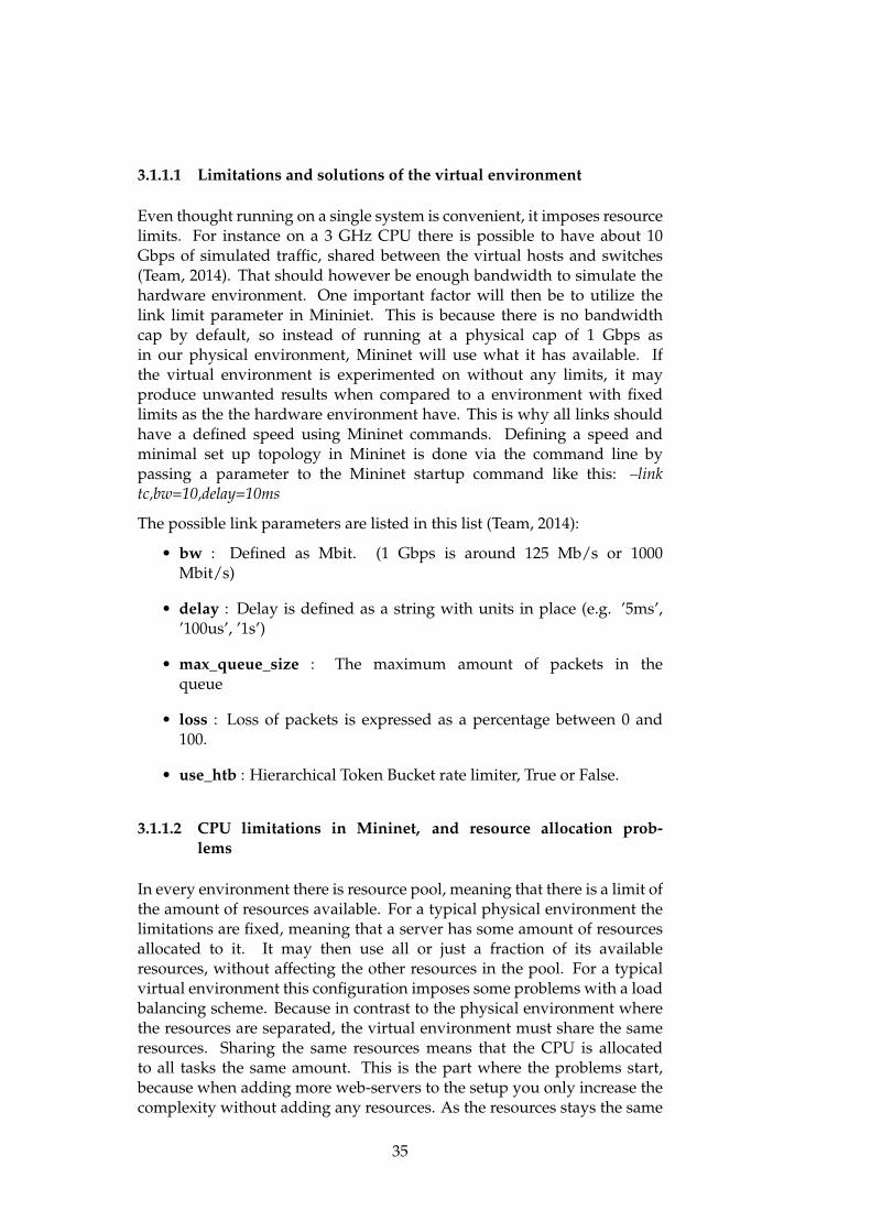
3.1.1.1 Limitations and solutions of the virtual environment

Even thought running on a single system is convenient, it imposes resourcelimits. For instance on a 3 GHz CPU there is possible to have about 10Gbps of simulated traffic, shared between the virtual hosts and switches(Team, 2014). That should however be enough bandwidth to simulate thehardware environment. One important factor will then be to utilize thelink limit parameter in Mininiet. This is because there is no bandwidthcap by default, so instead of running at a physical cap of 1 Gbps asin our physical environment, Mininet will use what it has available. Ifthe virtual environment is experimented on without any limits, it mayproduce unwanted results when compared to a environment with fixedlimits as the the hardware environment have. This is why all links shouldhave a defined speed using Mininet commands. Defining a speed andminimal set up topology in Mininet is done via the command line bypassing a parameter to the Mininet startup command like this: –linktc,bw=10,delay=10ms

The possible link parameters are listed in this list (Team, 2014):

• bw : Defined as Mbit. (1 Gbps is around 125 Mb/s or 1000Mbit/s)

• delay : Delay is defined as a string with units in place (e.g. ’5ms’,’100us’, ’1s’)

• max_queue_size : The maximum amount of packets in thequeue

• loss : Loss of packets is expressed as a percentage between 0 and100.

• use_htb : Hierarchical Token Bucket rate limiter, True or False.

3.1.1.2 CPU limitations in Mininet, and resource allocation prob-lems

In every environment there is resource pool, meaning that there is a limit ofthe amount of resources available. For a typical physical environment thelimitations are fixed, meaning that a server has some amount of resourcesallocated to it. It may then use all or just a fraction of its availableresources, without affecting the other resources in the pool. For a typicalvirtual environment this configuration imposes some problems with a loadbalancing scheme. Because in contrast to the physical environment wherethe resources are separated, the virtual environment must share the sameresources. Sharing the same resources means that the CPU is allocatedto all tasks the same amount. This is the part where the problems start,because when adding more web-servers to the setup you only increase thecomplexity without adding any resources. As the resources stays the same

35

and the complexity is increased, the overall performance is slower as youadd more servers, which is normally not a desired result.

To overcome this problem every virtual hosts in the Mininet environmentmust have a CPU limit parameter. We aim to achieve around 10 % CPUallocation for each host, this means that 1 server can throughput 10 percentof the CPU and 2 servers 20 percent. This means that when adding serversthe resource allocation works like a physical setup.

The suggested parameters for host configuration are finalised in thenetwork boot script, but below are the parameters just for CPU limit:

CPULimitedHost, sched=’cfs’, period_us=10000, cpu=.025

3.1.1.3 Configuring link parameters in Mininet

To closely mimic the physical network in our virtual environment, anetwork test measuring achievable bandwidth from the hardware is goingto be conducted. This test will involve the networking tool iperf forbandwidth throughput tests, and ping for a delay test. With these results,it is possible to set the link parameters so that the virtual network iscomparable to the physical one. The expected bw parameter is to be below,but close to 1000 Mbit/s and the delay less than 1 ms.

3.2 Hardware environment build

Building the hardware environment involved a more complicated setupthan originally planned for because of the inner workings of the F5 loadbalancer. However, this more complicated setup also connected it tothe Internet allowing for remote access and more controlled administra-tion.

3.2.1 Configuration of servers and clients

The final setup as shown in Figure 3.2, shows that some additions hadto be included to accommodate the policy’s of the BIG-IP 1600. Themain addition to the setup is the use of VLAN tagging, where as theservers and clients are on two different VLANs. A VLAN tag is a packetencapsulation mechanism of normal packets according to the IEEE 802.1Qstandard. Its main functionality is to virtually separate hosts in a networkfrom each other, for instance in a scenario where some clients are notallowed interaction with a specific server network. Because encapsulationis normally done in switches and because this setup does not have any,there was a problem with encapsulating the packets from the machinesconnected to F5 bridge. That is why the next section covers the steps on

36

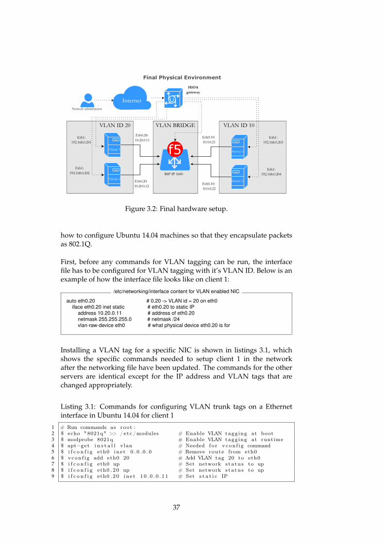
Figure 3.2: Final hardware setup.

how to configure Ubuntu 14.04 machines so that they encapsulate packetsas 802.1Q.

First, before any commands for VLAN tagging can be run, the interfacefile has to be configured for VLAN tagging with it’s VLAN ID. Below is anexample of how the interface file looks like on client 1:

/etc/networking/interface content for VLAN enabled NIC

auto eth0.20 # 0.20 -> VLAN id = 20 on eth0iface eth0.20 inet static # eth0.20 to static IP

address 10.20.0.11 # address of eth0.20netmask 255.255.255.0 # netmask /24vlan-raw-device eth0 # what physical device eth0.20 is for

Installing a VLAN tag for a specific NIC is shown in listings 3.1, whichshows the specific commands needed to setup client 1 in the networkafter the networking file have been updated. The commands for the otherservers are identical except for the IP address and VLAN tags that arechanged appropriately.

Listing 3.1: Commands for configuring VLAN trunk tags on a Ethernetinterface in Ubuntu 14.04 for client 1

1 # Run commands as root :2 $ echo "8021q" >> / etc /modules # Enable VLAN tagg ing at boot3 $ modprobe 8021q # Enable VLAN tagg ing at runtime4 $ apt−get i n s t a l l v lan # Needed f o r vcon f i g command5 $ i f c o n f i g eth0 i n e t 0 . 0 . 0 . 0 # Remove route from eth06 $ vcon f i g add eth0 20 # Add VLAN tag 20 to eth07 $ i f c o n f i g eth0 up # Set network s t a tu s to up8 $ i f c o n f i g eth0 .20 up # Set network s t a tu s to up9 $ i f c o n f i g eth0 .20 i n e t 1 0 . 0 . 0 . 1 1 # Set s t a t i c IP

37

3.2.2 GUI configuration of BIG-IP 1600

This section covers the parameters that were needed to configure the BIG-IP load balancer for load balancing and with proper routing. The BIG-IPhas one management (MGMT) port and four ports, which are numbered1.1, 1.2, 1.3 and 1.4. Where as the MGMT port is separated from the serverports, so that no traffic can cross between them. This means that for thefollowing configuration, some steps are configured after which port themachines is connected to. Which machine that is installed into which portsare as follows:

• 1.1: Client 1

• 1.2: Client 2

• 1.3: Server 1

• 1.4: Server 2

Which clients and servers that are installed on which ports are importantin regards to the VLAN setup of the BIG-IP. This is because they are goingto be on separated VLANs and the VLANs are tagged to specific ports.The two VLANs are public and private, with the private VLAN containingservers, and the public contain the clients.

• Private, VLAN tag = 10, subnet 10.0.0.0. Ports = 1.3, 1.4

• Public, VLAN tag = 20, subnet 10.20.0.0. Ports = 1.1, 1.2

Because VLANs are a separation of networks, they need to be bridged inorder to communicate together. This is done via the "Network ›› VLANs :VLAN Groups" menu where "create" is selected and these options are filledas shown in Figure 3.3

Finally to actually connect the BIG-IP to the network, we assign it a selfIP at 10.0.0.50 connected to the VLAN network bridge, bridge as shown inFigure 3.4. The configuration with how the separation of the VLANs worksand how they are connected are logically virtualized in figure 3.5. With theVLAN configured, everything is ready for the load balancing setup, whichis covered next.

3.2.2.1 BIG-IP Load Balance Setup

There are two parts needed to be setup for load balancing, which both area part of the Local Trafic settings of BIG-IP:

• Virtual IP: An IP clients queries for their requests, but not actuallybound to a server.

• Backend pool: The servers responding to a request sent to the virtualIP.

38

Log outHostname:IP Address:

emilload.master.no192.168.0.200

Date:Time:

Jan 4, 20022:08 AM (CET)

User:Role:

adminAdministrator Partition: Common

Main Help About

Unit: Active

Network ›› VLANs : VLAN Groups ›› bridge

General Properties

Configuration

Update Cancel Delete

Name bridge

Partition Common

VLANs

Members: Available:privatepublic <<

>>

Transparency Mode Translucent

Bridge All Traffic Enabled

Bridge In Standby Enabled

Migration Keepalive

MAC Masquerade

OverviewAccess statistics, performancegraphs, and links to helpful tools.

Templates and WizardsCreate common application trafficand system configurations.

Local TrafficControl the delivery of applicationtraffic for a local area network.

Network

Interfaces

Routes

Self IPs

Packet Filters

Rate Shaping

Spanning Tree

Trunks

Route Domains

VLANs

ARP

Properties Proxy Exclusion List

Figure 3.3: Configuration of networking bridge of the two VLANs in the F5GUI setup



Date:Time:

Jan 4, 20022:21 AM (CET)

User:Role:


Main Help About

Unit: Active

Network ›› Self IPs ›› 10.0.0.50

Configuration

Update Cancel Delete

IP Address 10.0.0.50

Partition Common

Netmask 255.255.255.0

VLAN bridge

Port Lockdown Allow Default



Local TrafficControl the delivery of applicationtraffic for a local area network.

Network

Interfaces

Routes

Self IPs

Packet Filters

Rate Shaping

Spanning Tree

Trunks

Route Domains

VLANs

ARP

Properties

Figure 3.4: Configuration of self IP in the F5 GUI setup

The settings for the Backend Pool is found under the menu "Local Traffic ››Pools : Pool List" which covers the backend (pool) setup. In this example,even though the name of the pool can be generic it is named "Backend-servers". Here there are two parts that completes the pool, the propertiesof the pool and the members it have. The first settings page as shown in

39

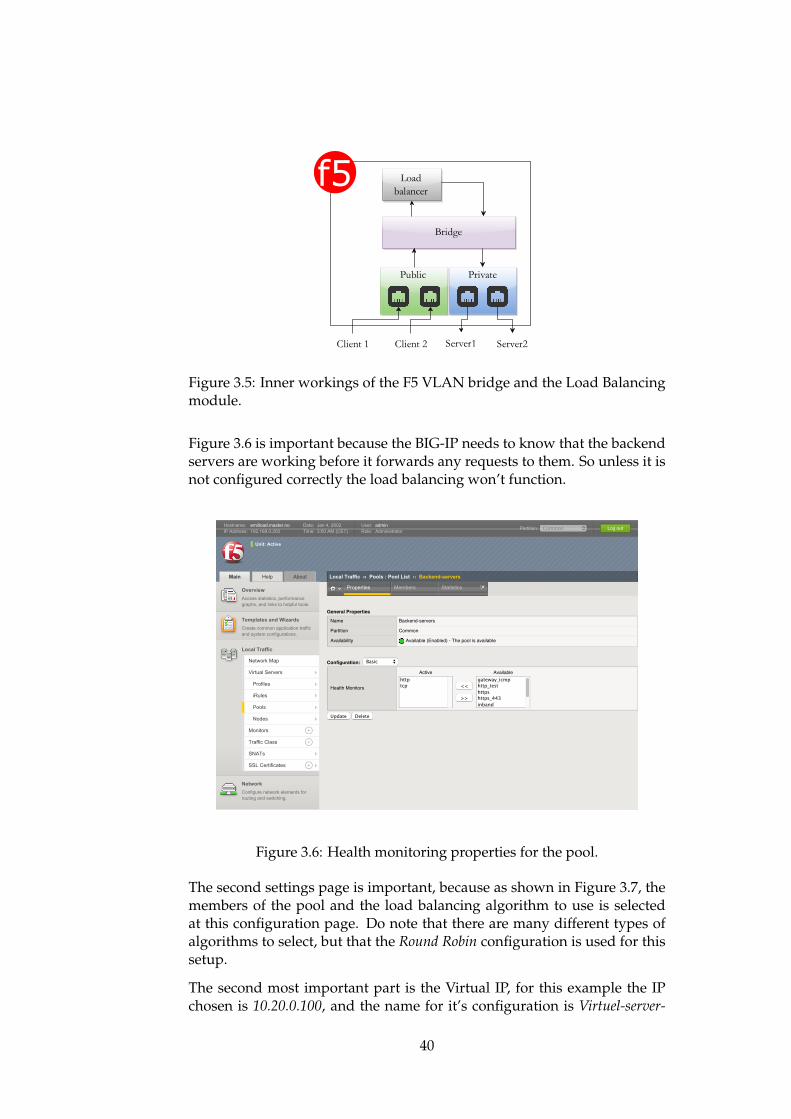
Figure 3.5: Inner workings of the F5 VLAN bridge and the Load Balancingmodule.

Figure 3.6 is important because the BIG-IP needs to know that the backendservers are working before it forwards any requests to them. So unless it isnot configured correctly the load balancing won’t function.



Date:Time:

Jan 4, 20023:00 AM (CET)

User:Role:


Main Help About

Unit: Active

Local Traffic ›› Pools : Pool List ›› Backendservers

General Properties

Configuration: Basic

Update Delete

Name Backend-servers

Partition Common

Availability Available (Enabled) - The pool is available

Health Monitors

Active Availablehttptcp <<

>>

gateway_icmphttp_testhttpshttps_443inbandtcp_half_openudp



Local Traffic

NetworkConfigure network elements forrouting and switching.

Network Map

Virtual Servers

Profiles

iRules

Pools

Nodes

Monitors

Traffic Class

SNATs

SSL Certificates

Properties Members Statistics

Figure 3.6: Health monitoring properties for the pool.

The second settings page is important, because as shown in Figure 3.7, themembers of the pool and the load balancing algorithm to use is selectedat this configuration page. Do note that there are many different types ofalgorithms to select, but that the Round Robin configuration is used for thissetup.

The second most important part is the Virtual IP, for this example the IPchosen is 10.20.0.100, and the name for it’s configuration is Virtuel-server-

40



Date:Time:

Jan 4, 20022:46 AM (CET)

User:Role:


Main Help About

Unit: Active

Local Traffic ›› Pools : Pool List ›› Backendservers

Load Balancing

Update

Current Members Add...

Enable Disable Remove

Load Balancing Method Round Robin

Priority Group Activation Disabled

Status Member Node Name Ratio Priority Group Connection Limit

10.0.0.21:80 server1 1 0 (Active) 0

10.0.0.22:80 server2 1 0 (Active) 0

Overview


Local Traffic

Welcome

Traffic Summary

Performance

Statistics

Dashboard

Network Map

Virtual Servers

Profiles

iRules

Pools

Nodes

Monitors

Traffic Class

SNATs

Properties Members Statistics

Figure 3.7: Pool members and load balancing algorithm.

100. Do note that the IP is part of the public VLAN as that is where theclients are connected, as they are the machines that will be using the VirtualIP. The complete set up for this is shown in Figure 3.8, which is the firstsettings page. Here it is configured for Standard load balancing on port 80,but other ports or protocols can be selected. The second page "resources"is not shown, but on this page the backend "Backend-servers" is selected asthose servers should respond to requests at this virtual IP.

3.3 Load Balancing methodology for SDN

As discussed in the background section, there have been two differentapproaches to SDN-based load balancing because of limitations to thedifferent methods.

Reactive gives more fine grained control, but are limited by the processingpower of the controller and slowing down every request. In contrast toproactive that gives less control, but limits the use of processing power andrequest completion time. Depending on the network, using both modes fordifferent setups/services may be beneficial. As for some services it maybe acceptable with higher strain on the controller if it copes with networkchanges better. Finding out how the two modes behave will be part ofthe process of determining how SDN-based load balancing functions incomparison to a hardware solution.

41

Log outHostname:

IP Address:

emilload.master.no

192.168.0.200

Date:

Time:

May 6, 2015

12:20 AM (CEST)

User:

Role:

admin

AdministratorPartition: Common

Main Help About

Unit: Active

Local Traffic ›› Virtual Servers : Virtual Server List ›› Virtuelserver100

General Properties

Configuration: Basic

Name Virtuel-server-100

Partition Common

DestinationType: Host NetworkAddress: 10.20.0.100

Service Port 80 HTTP

Availability

State Enabled

Type Standard

Protocol TCP

OneConnect Profile None

NTLM Conn Pool None

HTTP Profile None

FTP Profile None

SSL Profile (Client) None

SSL Profile (Server) None

Overview

Access statistics, performance

graphs, and links to helpful tools.

Templates and Wizards

Create common application traffic

and system configurations.

Local Traffic

Network

Configure network elements for

routing and switching.

Network Map

Virtual Servers

Profiles

iRules

Pools

Nodes

Monitors

Traffic Class

SNATs

SSL Certificates

Properties Resources Statistics

Figure 3.8: Virtual IP settings page.

3.4 Comparing SDN controller solutions

The first problem statement bases itself on finding an SDN-based solutionto load balancing, but as there are multiple solutions there is no wayof knowing beforehand which is the most feasible. That is why twocontrollers approaches to SDN load balancing be tested. Sourcing theavailable controllers that come with load balancing capabilities, whileexcluding any commercial controllers, have determined which controllersto test. From here it is clear that because the way a reactive solution works,it introduces some network delay in any SDN solution. Testing more thantwo controllers would therefore not be necessary unless these tests show alarge variation in performance.

3.4.1 POX SDN controller

POX has been chosen over NOX as it is the latest controller for scientificresearch recommended by the developers of both controllers. As POX isPython-based, it officially requires Python 2.7. Newest version is the eelbranch which is available at GitHub, but the carp version that ships withMininet is updated. This means that the latest branch will need to bemanual downloaded and used for tests in this thesis. The default port for aPOX controller is 6633 which therefore should be included in the mn startupcommand. The startup command is described in the 3.1.1 section. POXcan be started as a l2 learning switch SDN controller with the followingterminal command:

42

POX start

./pox.py forwarding.l2_learning

Multiple modules can be specified like this:POX multiple modules

./pox.py samples.pretty_log forwarding.l2_learning

Inputs to the modules are also possible via parameters:POX module input

./pox.py log.level --DEBUG forwarding.l2_learning

To run the POX controller with the load balancer module, the followingcommand should be executed from the pox directory. Do note that –ip isfor the virtual server address and the –servers parameter is for the actualservers. There are no port options as this load balancer works in Networklayer of the OSI model as shown in Figure 2.1.

POX load balancer example

./pox.py misc.ip_loadbalancer --ip=10.1.2.3 --servers=10.0.0.1,10.0.0.2

3.4.2 Floodlight SDN controller

Floodlight has been chosen as the second SDN controller as it also comeswith a reactive load balancing algorithm. It is available at GitHub fordownload and requires JDK, Ant, Python and Eclipse that can be installedby the steps outlined in listings 3.2

Listing 3.2: Install and run Floodlight1 $ sudo apt−get i n s t a l l bui ld−e s s e n t i a l de fau l t−jdk ant python−dev

↪→ e c l i p s e2 $ g i t c l one g i t : // github . com/ f l o o d l i g h t / f l o o d l i g h t . g i t3 $ cd f l o o d l i g h t4 $ g i t checkout s t ab l e5 $ ant ;6 $ sudo mkdir /var / l i b / f l o o d l i g h t7 $ sudo chmod 777 /var / l i b / f l o o d l i g h t8 # Running the c o n t r o l l e r i s done by with the f o l l ow i ng command :9 $ java − j a r t a r g e t / f l o o d l i g h t . j a r

10 # GUI i s at : http :// l o c a l h o s t :8080/ u i / index . html

Default port for Floodlight is port 6653, so running a minimal Mininettopology is done with the command bellow:

Mininet minimal for Floodlight

sudo mn --controller=remote,ip=127.0.0.1,port=6653

When the controller is running, configuring for load balancing is doneusing the REST API which is pushed to the controller using curl (HTTP)commands. The commands should be run via a script as shown in 3.3(Wang, 2012)

43

Listing 3.3: Configure load balancing1 #!/ bin / sh2 cu r l −X POST −d ’{ " id " : "1" , "name" : " vip1 " , " p ro to co l " : " tcp " , " address " : "

↪→ 1 0 . 0 . 0 . 1 0 0 " , " port " : "80" } ’ http :// l o c a l h o s t :8080/quantum/v1 .0/↪→ v ips /

3 cu r l −X POST −d ’{ " id " : "1" , "name" : " pool " , " p ro to co l " : " tcp " , "vip_id" : "1"↪→ } ’ http :// l o c a l h o s t :8080/quantum/v1 .0/ poo l s /

4 cu r l −X POST −d ’{ " id " : "2" , " address " : " 1 0 . 0 . 0 . 3 " , " port " : "80" , "pool_id" :↪→ "1" } ’ http :// l o c a l h o s t :8080/ quantum/v1 .0/members/

5 cu r l −X POST −d ’{ " id " : "3" , " address " : " 1 0 . 0 . 0 . 4 " , " port " : "80" , "pool_id" :↪→ "1" } ’ http :// l o c a l h o s t :8080/ quantum/v1 .0/members/

This script 3.3, will setup a round-robin load balancing algorithm basedon connections for the virtual IP 10.0.0.100 at port 80 with two servers inthe back end pool. As a notation for the default settings for Floodlight,it loads many modules that can be seen in Figure 2.9. Reducing theamount of loaded modules, by removing the unused ones may improvethe performance of this controller.

3.5 Experiments methodology

This sections breaks down the problem statement into tasks that needs tobe completed and in the order they should happen in order to answer theproblems statements.

1. Build and configure the hardware environment, which is alreadycovered in the approach section.

2. Benchmark the hardware environment for baseline results

3. Determine link speed (bandwidth) parameter for virtual environ-ment from hardware tests.

4. Build and configure the virtual environment

5. Benchmark reactive SDN solutions (POX vs Floodlight) using anautomated Mininet high-level CLI approach.

6. Develop a proactive solution with focus on performance

3.6 Experiments Evaluation

The results gathered should be done so after an intent of what parameterswe are searching for. This section covers these results.

3.6.1 Evaluating the performance of the solutions

Evaluation of performance is done in a client/server relationship. It istherefore necessary to run both client and server software. However,

44

there are not many complete solutions in the benchmarking world ofclient/server relationships. The most widespread ones are over the HTTPprotocol, like the benchmarking tools httperf and ab.

Due to the environments not being fully comparable the numbers gatheredcannot be directly compared. This is due to the fact that the systemresources differ between the environments, meaning that doing baselineversus improvement of both systems in is a more sane methodology.

The tests are needed to determine the improvement for the load balancingscheme in comparison to not running one for both environments. Thismeans that we must do performance test of both systems running HTTP-servers. To find out how does not using load-balance compare to usingload-balance. I.E for SDN test using only load balancing algorithm andthen forward algorithm.

For the httperf tests, what defines its rate limit; e.g when is a setupperforming at max capacity, will be when the requested rate is no longerthe same as the response rate. When defining parameters for httperf, itis intended to set the number of connections to a number that matchesaround 60 seconds for the test to complete. This is to ensure that the testsare more reliable than using short burst tests at only a few seconds. Theactual performance parameters we are looking for are summarized in thislist:

• Baseline results: How does Physical, POX and Floodlight handle nor-mal switch behavior? Main parameter is: Requests per Second.

– For virtual only: How does the Open vSwitch handle switch-ing?

• Load Balancing results: How does the three setups handle loadbalancing?

• Is there an impact on the performance if there is small or large filesbeing transferred?

3.6.2 Evaluating the scalability of the solutions

The performance of the systems is only part of what we aim to discoverduring our research, as another important part is the scalability of thesolutions. To fully answer if the solutions are feasible, how they scale withincreased resources is necessary. Like for instance that there is not any hardlimitations associated with the solution. A hard limit is where the systemfails to increase its performance even though it has increased resources. Forexample in a scenario where the application fails at a request rate of 50, itdoes then have some hard limit in it’s programing, and therefore increasingthe resources would not increase the rate above this number.

45

• For the virtual environment these are the questions we want toanswer for the scalability of SDN:

– How is the system resources used in addition to the throughputnumber of HTTP connections? Here we want to answer whatis stealing the most CPU of the virtual environment? As it maybe server software, benchmark software, Open vSwitch or thecontroller application. Finding the culprit could answer how thevirtual environment would scale in a real environment.

3.7 Experiments

This section covers the exact test that are going to be conducted, that are indirect correlation with answering the problem statement. Other tests thatare used to define network parameters are not listed here.

1. Small HTTP page test for all setups: Physical, POX(proactive/reactive),Floodlight(proactive/reactive)

(a) httperf and ab test of baseline (1 server).

(b) httperf and ab test of load balancing (2 servers).

(c) When necessary, e.g results from test 1-2 does not show a result:load balancing (3 server).

2. Large load e.g big file transfer test for all setups: Physical,POX(proactive/reactive), Floodlight(proactive/reactive)

(a) httperf and ab test of baseline (1server)

(b) httperf test of load balancing (2 servers)

(c) When necessary, e.g results from test 1-2 does not show a result:load balancing (3 server).

46

Part III

Conclusion

47

Chapter 4

Results and Analysis

In this chapter the results of the approach is presented. It contains the datacollected from performance tests measured on both environments, as wellas the analysis.

4.1 Results of initial link performance tests

As shown in Figure 3.2 the setup have two networks, one routed througha normal switch and one through the BIG-IP. This test is primarily aboutfinding out what the actual link speed and latency of the physical links are,in order to set equivalent parameters in Mininet. However, as the BIG-IPlacks specialized hardware it is going to affect the performance. How theperformance is affected is only discovered by testing a normal switch inaddition to the BIG-IP unit. That is why routing through a switch will alsobe tested as a comparison.

4.1.0.1 Latency

Latency, measured in ms have been tested using the ping command with-c parameter 100 in Linux and a average score have been calculated andplotted into Figure 4.1 for both routes.

4.1.0.2 Network throughput

Network throughput, measured in Mbit/s have been tested using the iperfcommand. However, because of the network latency delay in the BIG-IPit needs more concurrent connections than what one iperf test generates toreach it’s maximum. This means that multiple iperf tests must be issued atthe same time to find the limit. By running those multiple iperf tests wefound out that the limit for one link is around 700 Mbit/s, but the BIG-IPcan route more than this simultaneously, up to ≈ 1200 Mbit/s. But when all

49

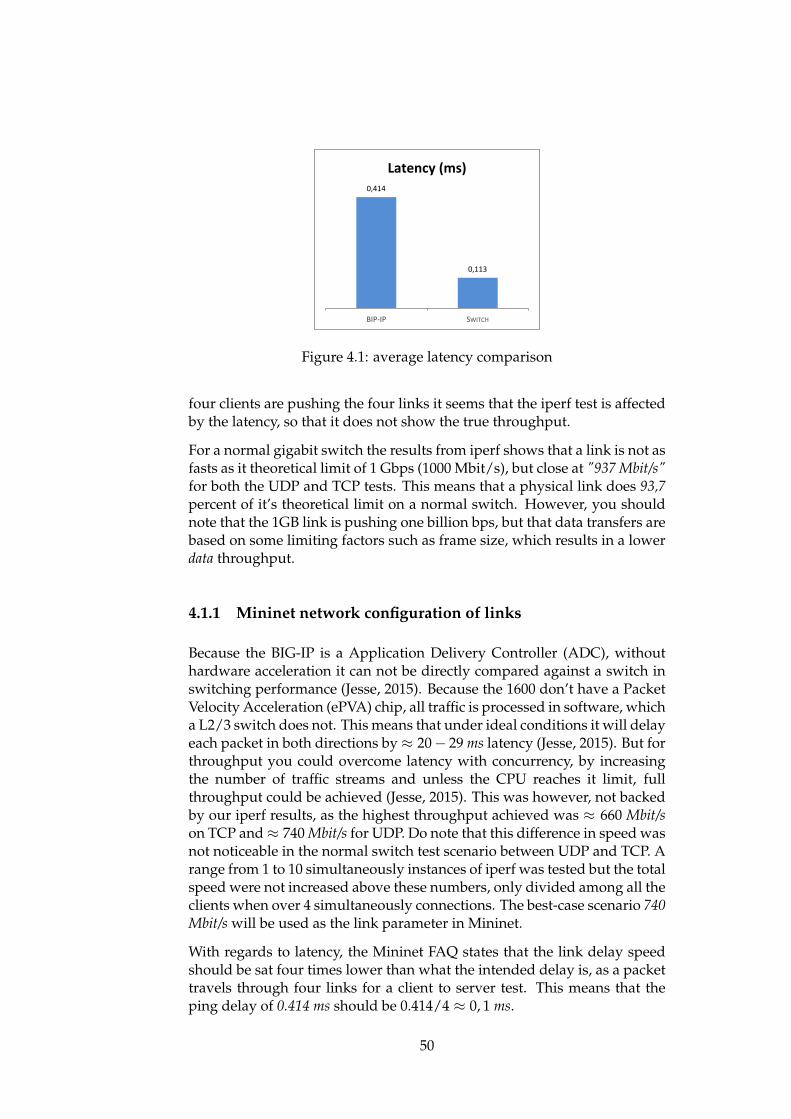
0,414

0,113

BIP-‐IP SWITCH

Latency (ms)

Figure 4.1: average latency comparison

four clients are pushing the four links it seems that the iperf test is affectedby the latency, so that it does not show the true throughput.

For a normal gigabit switch the results from iperf shows that a link is not asfasts as it theoretical limit of 1 Gbps (1000 Mbit/s), but close at "937 Mbit/s"for both the UDP and TCP tests. This means that a physical link does 93,7percent of it’s theoretical limit on a normal switch. However, you shouldnote that the 1GB link is pushing one billion bps, but that data transfers arebased on some limiting factors such as frame size, which results in a lowerdata throughput.

4.1.1 Mininet network configuration of links

Because the BIG-IP is a Application Delivery Controller (ADC), withouthardware acceleration it can not be directly compared against a switch inswitching performance (Jesse, 2015). Because the 1600 don’t have a PacketVelocity Acceleration (ePVA) chip, all traffic is processed in software, whicha L2/3 switch does not. This means that under ideal conditions it will delayeach packet in both directions by≈ 20− 29 ms latency (Jesse, 2015). But forthroughput you could overcome latency with concurrency, by increasingthe number of traffic streams and unless the CPU reaches it limit, fullthroughput could be achieved (Jesse, 2015). This was however, not backedby our iperf results, as the highest throughput achieved was ≈ 660 Mbit/son TCP and≈ 740 Mbit/s for UDP. Do note that this difference in speed wasnot noticeable in the normal switch test scenario between UDP and TCP. Arange from 1 to 10 simultaneously instances of iperf was tested but the totalspeed were not increased above these numbers, only divided among all theclients when over 4 simultaneously connections. The best-case scenario 740Mbit/s will be used as the link parameter in Mininet.

With regards to latency, the Mininet FAQ states that the link delay speedshould be sat four times lower than what the intended delay is, as a packettravels through four links for a client to server test. This means that theping delay of 0.414 ms should be 0.414/4 ≈ 0, 1 ms.

50

4.1.1.1 Parameters tested versus the real parameters

To check that the suggested theoretical parameters from the tests matchup to the correct parameters in Mininet, they where tested and adjustedaccordingly. The test results shows that in order to achieve ≈ 740 Mbit/s inMininet, the link parameter bw should be sat to 820, and for the delay tomatch it must be 0,07 ms.

4.1.2 Mininet CPU limits

In a virtual environment like Mininet the CPU is by default shared equallybetween the hosts, switches and the controller in the network after demand.This is however not valid for a performance test where the amount ofservers increase. The reason behind this is that they share the same amountof resources. So by increasing the amount of servers, we are only increasingthe complexity of the system without increasing the capacity, which is thecomplete opposite of what load balancing aims to achieve. Because thiswas shown in early performance tests, a CPU limit has therefore beenenforced in the run-time scripts as shown in the next section. The goalfor the CPU limits is around 10 % CPU utilization for each host, this meansthat when increasing the amount of servers the resource pool is actuallyincreased.

4.1.3 Mininet configuration file for run-time parameters

To automate the setup of the virtual environment, a Mininet high-levelpython CLI file has been developed. This script when run, initializes thevirtual environment with the correct link parameters, the correct controllermodules, the hosts and the server applications if wanted. This file is shownin Appendix A.1, and is started with the command sudo python poxfile.py forthe POX version.

The other version is for the Floodlight controller, as shown in AppendixA.2. It is basically the same as the POX version expect that it is tailored foranother controller, namely the Floodlight controller. It is started with thesame command, with only the name of the file being different: sudo pythonfloodfile.py.

These scripts may also take other commands as parameters, for instancelike starting a httperf of ab benchmark of the environment. An example ofdoing so is shown in the POX Appendix A.1.

51

4.2 Performance test results for the physical environ-ment

This section covers the results gathered from the performance testsexecuted for the different scenarios as outlined in the approach. The resultsgathered from the physical environment is presented in this section. Thereare five test scenarios:

1. BIG-IP acting as switch from host to one server.

2. BIG-IP acting as a load balancer for one server.

3. BIG-IP acting as a load balancer for two servers.

4. BIG-IP acting as a load balancer for three servers.

5. BIG-IP saturation point.

4.2.1 httperf tests

For the httperf test, it was unable to find the saturation point due to the factthat it exits with error code "*** buffer overflow detected ***: httperf terminated"when running the following command, which generates less traffic than thesystem maximum:

httperf command at overflow parameters

httperf --server 10.20.0.100 --uri ’/index.html’ --num-conn 13680 --num-call 100 --rate 228 --timeout 5

Do note that this was for a custom version of httperf, as the Ubuntupackaged version fails with different error related to maximum number ofopen file descriptors, at even lower loads. The error message the Ubuntuversion outputs, is attached below:

httperf error in version from Ubuntu repository (0.9.0-2)

httperf: warning: open file limit > FD_SETSIZE; limiting max. # of open files to FD_SETSIZE

This means that no valid httperf test could be gathered from the physicalenvironment, as the software has errors in it.

4.2.2 ab tests

This section covers the gathered results from benchmarking the physicalenvironment with the benchmarking tool ab. The BIG-IP can run differentforwarding options for load balancing, but the standard option have beenselected for the tests.

52

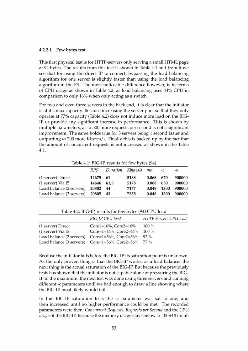
4.2.2.1 Few bytes test

This first physical test is for HTTP-servers only serving a small HTML pageat 94 bytes. The results from this test is shown in Table 4.1 and from it wesee that for using the direct IP to connect, bypassing the load balancingalgorithm for one server is slightly faster than using the load balancingalgorithm in the F5. The most noticeable difference however, is in termsof CPU usage as shown in Table 4.2, as load balancing uses 44% CPU incomparison to only 16% when only acting as a switch.

For two and even three servers in the back end, it is clear that the initiatoris at it’s max capacity. Because increasing the server pool so that they onlyoperate at 77% capacity (Table 4.2) does not induce more load on the BIG-IP or provide any significant increase in performance. This is shown bymultiple parameters, as ≈ 500 more requests per second is not a significantimprovement. The same holds true for 3 servers being 1 second faster andoutputting ≈ 200 more Kbytes/s. Finally this is backed up by the fact thatthe amount of concurrent requests is not increased as shown in the Table4.1.

Table 4.1: BIG-IP, results for few bytes (94)

RPS Duration Kbytes/s ms -c -n

(1 server) Direct 14675 61 5188 0.068 670 900000(1 server) Via f5 14646 61,5 5178 0.068 650 900000Load balance (2 servers) 20302 44 7177 0.049 1300 900000Load balance (3 servers) 20805 43 7355 0.048 1300 900000

Table 4.2: BIG-IP, results for few bytes (94) CPU load

BIG-IP CPU load HTTP Servers CPU load:

(1 server) Direct Core1=16%, Core2=16% 100 %(1 server) Via f5 Core=1=44%, Core2=44% 100 %Load balance (2 servers) Core=1=56%, Core2=56% 92 %Load balance (3 servers) Core=1=56%, Core2=56% 77 %

Because the initiator fails before the BIG-IP its saturation point is unknown.As the only proven thing is that the BIG-IP works, as a load balancer thenext thing is the actual saturation of the BIG-IP. But because the previouslytests has shown that the initiator is not capable alone of pressuring the BIG-IP to the maximum, the next test was done using three servers and runningdifferent -c parameters until we had enough to draw a line showing wherethe BIG-IP most likely would fail.

In this BIG-IP saturation tests the -c parameter was sat to one, andthen increased until no higher performance could be met. The recordedparameters were then: Concurrent Requests, Requests per Second and the CPUusage of the BIG-IP. Because the memory usage stays below≈ 100MB for all

53

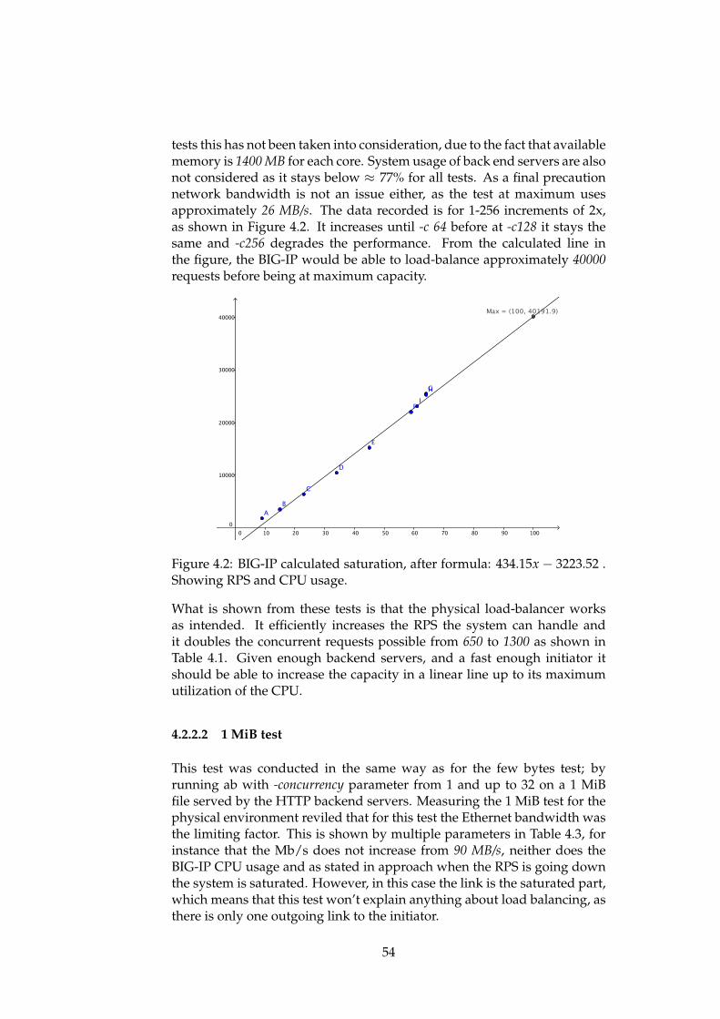
tests this has not been taken into consideration, due to the fact that availablememory is 1400 MB for each core. System usage of back end servers are alsonot considered as it stays below ≈ 77% for all tests. As a final precautionnetwork bandwidth is not an issue either, as the test at maximum usesapproximately 26 MB/s. The data recorded is for 1-256 increments of 2x,as shown in Figure 4.2. It increases until -c 64 before at -c128 it stays thesame and -c256 degrades the performance. From the calculated line inthe figure, the BIG-IP would be able to load-balance approximately 40000requests before being at maximum capacity.

0 10 20 30 40 50 60 70 80 90 1000

10000

20000

30000

40000

a

AB

C

D

E

F

GH

I

Max = (100, 40191.9)

Figure 4.2: BIG-IP calculated saturation, after formula: 434.15x− 3223.52 .Showing RPS and CPU usage.

What is shown from these tests is that the physical load-balancer worksas intended. It efficiently increases the RPS the system can handle andit doubles the concurrent requests possible from 650 to 1300 as shown inTable 4.1. Given enough backend servers, and a fast enough initiator itshould be able to increase the capacity in a linear line up to its maximumutilization of the CPU.

4.2.2.2 1 MiB test

This test was conducted in the same way as for the few bytes test; byrunning ab with -concurrency parameter from 1 and up to 32 on a 1 MiBfile served by the HTTP backend servers. Measuring the 1 MiB test for thephysical environment reviled that for this test the Ethernet bandwidth wasthe limiting factor. This is shown by multiple parameters in Table 4.3, forinstance that the Mb/s does not increase from 90 MB/s, neither does theBIG-IP CPU usage and as stated in approach when the RPS is going downthe system is saturated. However, in this case the link is the saturated part,which means that this test won’t explain anything about load balancing, asthere is only one outgoing link to the initiator.

54

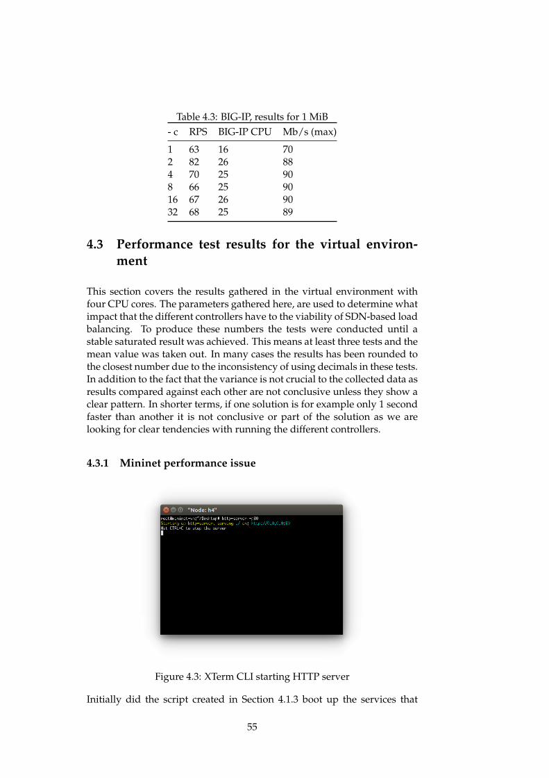
Table 4.3: BIG-IP, results for 1 MiB- c RPS BIG-IP CPU Mb/s (max)

1 63 16 702 82 26 884 70 25 908 66 25 9016 67 26 9032 68 25 89

4.3 Performance test results for the virtual environ-ment

This section covers the results gathered in the virtual environment withfour CPU cores. The parameters gathered here, are used to determine whatimpact that the different controllers have to the viability of SDN-based loadbalancing. To produce these numbers the tests were conducted until astable saturated result was achieved. This means at least three tests and themean value was taken out. In many cases the results has been rounded tothe closest number due to the inconsistency of using decimals in these tests.In addition to the fact that the variance is not crucial to the collected data asresults compared against each other are not conclusive unless they show aclear pattern. In shorter terms, if one solution is for example only 1 secondfaster than another it is not conclusive or part of the solution as we arelooking for clear tendencies with running the different controllers.

4.3.1 Mininet performance issue

Figure 4.3: XTerm CLI starting HTTP server

Initially did the script created in Section 4.1.3 boot up the services that

55

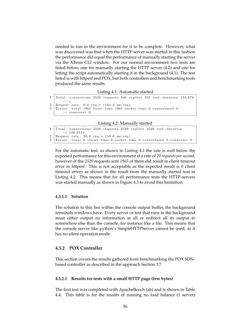
needed to run in the environment for it to be complete. However, whatwas discovered was that when the HTTP server was started in this fashionthe performance did equal the performance of manually starting the servervia the XTerm CLI window. For our normal environment two tests arelisted below, one for manually starting the HTTP server (4.2) and one forletting the script automatically starting it in the background (4.1). The testlisted is with httperf and POX, but both controllers and benchmarking toolsproduced the same results.

Listing 4.1: Automatic started1 Total : connect i ons 2520 r eque s t s 830 r e p l i e s 555 te s t−durat ion 133.878

↪→ s2 Request ra t e : 6 . 2 req / s (161 . 3 ms/ req )3 Errors : t o t a l 1965 l i e n t−timo 1965 socket−timo 0 connre fused 0

↪→ connre se t 0

Listing 4.2: Manually started1 Total : connect i ons 2520 r eque s t s 2520 r e p l i e s 2520 te s t−durat ion

↪→ 126.051 s2 Request ra t e : 20 .0 req / s ( 50 . 0 ms/ req )3 Errors : t o t a l 0 c l i e n t−timo 0 socket−timo 0 connre fused 0 connre se t 0

For the automatic test, as shown in Listing 4.1 the rate is well below theexpected performance for this environment at a rate of 20 requests per second,however of the 2520 requests sent 1965 of them did result in client timeouterror in httperf. This is not acceptable as the expected result is 0 clienttimeout errors as shown in the result from the manually started test inListing 4.2. This means that for all performance tests the HTTP-serverswas started manually as shown in Figure 4.3 to avoid this limitation.

4.3.1.1 Solution

The solution to this lies within the console output buffer, the backgroundterminals windows have. Every server or test that runs in the backgroundmust either output no information at all or redirect all its output tosomewhere else than the console, for instance like a file. This means thatthe console server like python’s SimpleHTTPServer cannot be used, as ithas no silent operation mode.

4.3.2 POX Controller

This section covers the results gathered form benchmarking the POX SDN-based controller as described in the approach Section 3.7.

4.3.2.1 Results for tests with a small HTTP page (few bytes)

The first test was completed with ApacheBench (ab) and is shown in Table4.4. This table is for the results of running no load balance (1 server)

56

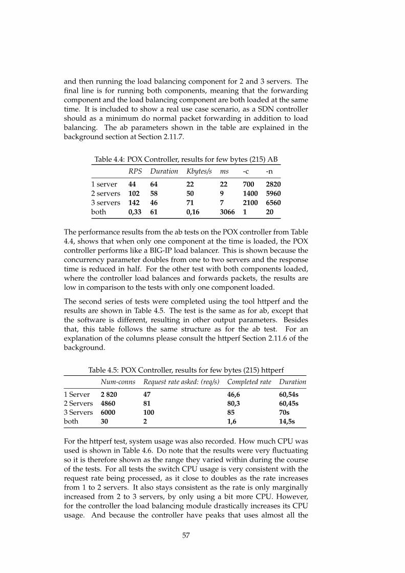
and then running the load balancing component for 2 and 3 servers. Thefinal line is for running both components, meaning that the forwardingcomponent and the load balancing component are both loaded at the sametime. It is included to show a real use case scenario, as a SDN controllershould as a minimum do normal packet forwarding in addition to loadbalancing. The ab parameters shown in the table are explained in thebackground section at Section 2.11.7.

Table 4.4: POX Controller, results for few bytes (215) AB


1 server 44 64 22 22 700 28202 servers 102 58 50 9 1400 59603 servers 142 46 71 7 2100 6560both 0,33 61 0,16 3066 1 20

The performance results from the ab tests on the POX controller from Table4.4, shows that when only one component at the time is loaded, the POXcontroller performs like a BIG-IP load balancer. This is shown because theconcurrency parameter doubles from one to two servers and the responsetime is reduced in half. For the other test with both components loaded,where the controller load balances and forwards packets, the results arelow in comparison to the tests with only one component loaded.

The second series of tests were completed using the tool httperf and theresults are shown in Table 4.5. The test is the same as for ab, except thatthe software is different, resulting in other output parameters. Besidesthat, this table follows the same structure as for the ab test. For anexplanation of the columns please consult the httperf Section 2.11.6 of thebackground.

Table 4.5: POX Controller, results for few bytes (215) httperf

Num-conns Request rate asked: (req/s) Completed rate Duration

1 Server 2 820 47 46,6 60,54s2 Servers 4860 81 80,3 60,45s3 Servers 6000 100 85 70sboth 30 2 1,6 14,5s

For the httperf test, system usage was also recorded. How much CPU wasused is shown in Table 4.6. Do note that the results were very fluctuatingso it is therefore shown as the range they varied within during the courseof the tests. For all tests the switch CPU usage is very consistent with therequest rate being processed, as it close to doubles as the rate increasesfrom 1 to 2 servers. It also stays consistent as the rate is only marginallyincreased from 2 to 3 servers, by only using a bit more CPU. However,for the controller the load balancing module drastically increases its CPUusage. And because the controller have peaks that uses almost all the

57

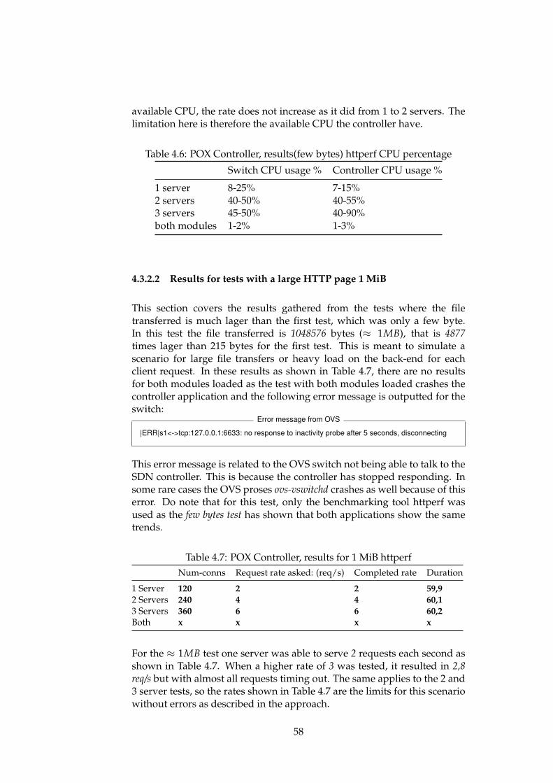
available CPU, the rate does not increase as it did from 1 to 2 servers. Thelimitation here is therefore the available CPU the controller have.

Table 4.6: POX Controller, results(few bytes) httperf CPU percentage

Switch CPU usage % Controller CPU usage %

1 server 8-25% 7-15%2 servers 40-50% 40-55%3 servers 45-50% 40-90%both modules 1-2% 1-3%

4.3.2.2 Results for tests with a large HTTP page 1 MiB

This section covers the results gathered from the tests where the filetransferred is much lager than the first test, which was only a few byte.In this test the file transferred is 1048576 bytes (≈ 1MB), that is 4877times lager than 215 bytes for the first test. This is meant to simulate ascenario for large file transfers or heavy load on the back-end for eachclient request. In these results as shown in Table 4.7, there are no resultsfor both modules loaded as the test with both modules loaded crashes thecontroller application and the following error message is outputted for theswitch:

Error message from OVS

|ERR|s1<->tcp:127.0.0.1:6633: no response to inactivity probe after 5 seconds, disconnecting

This error message is related to the OVS switch not being able to talk to theSDN controller. This is because the controller has stopped responding. Insome rare cases the OVS proses ovs-vswitchd crashes as well because of thiserror. Do note that for this test, only the benchmarking tool httperf wasused as the few bytes test has shown that both applications show the sametrends.

Table 4.7: POX Controller, results for 1 MiB httperfNum-conns Request rate asked: (req/s) Completed rate Duration

1 Server 120 2 2 59,92 Servers 240 4 4 60,13 Servers 360 6 6 60,2Both x x x x

For the ≈ 1MB test one server was able to serve 2 requests each second asshown in Table 4.7. When a higher rate of 3 was tested, it resulted in 2,8req/s but with almost all requests timing out. The same applies to the 2 and3 server tests, so the rates shown in Table 4.7 are the limits for this scenariowithout errors as described in the approach.

58

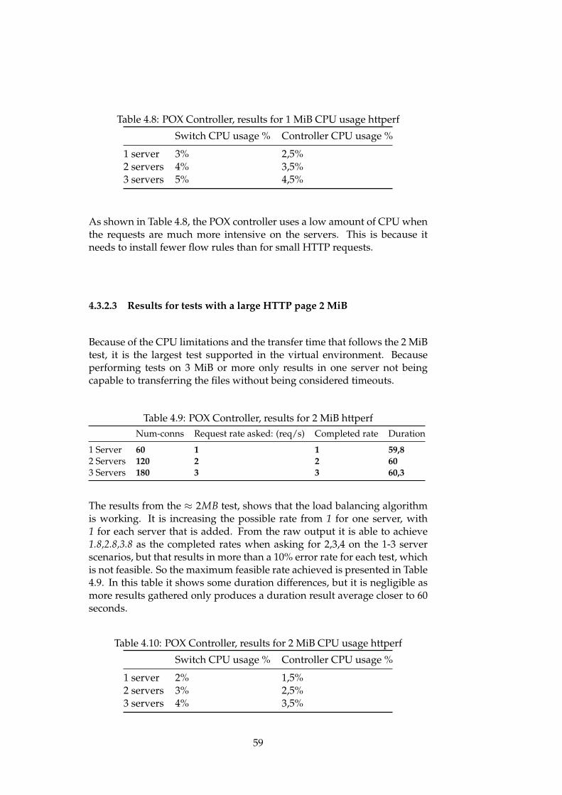
Table 4.8: POX Controller, results for 1 MiB CPU usage httperf


1 server 3% 2,5%2 servers 4% 3,5%3 servers 5% 4,5%

As shown in Table 4.8, the POX controller uses a low amount of CPU whenthe requests are much more intensive on the servers. This is because itneeds to install fewer flow rules than for small HTTP requests.

4.3.2.3 Results for tests with a large HTTP page 2 MiB

Because of the CPU limitations and the transfer time that follows the 2 MiBtest, it is the largest test supported in the virtual environment. Becauseperforming tests on 3 MiB or more only results in one server not beingcapable to transferring the files without being considered timeouts.

Table 4.9: POX Controller, results for 2 MiB httperfNum-conns Request rate asked: (req/s) Completed rate Duration

1 Server 60 1 1 59,82 Servers 120 2 2 603 Servers 180 3 3 60,3

The results from the ≈ 2MB test, shows that the load balancing algorithmis working. It is increasing the possible rate from 1 for one server, with1 for each server that is added. From the raw output it is able to achieve1.8,2.8,3.8 as the completed rates when asking for 2,3,4 on the 1-3 serverscenarios, but that results in more than a 10% error rate for each test, whichis not feasible. So the maximum feasible rate achieved is presented in Table4.9. In this table it shows some duration differences, but it is negligible asmore results gathered only produces a duration result average closer to 60seconds.

Table 4.10: POX Controller, results for 2 MiB CPU usage httperf


1 server 2% 1,5%2 servers 3% 2,5%3 servers 4% 3,5%

59

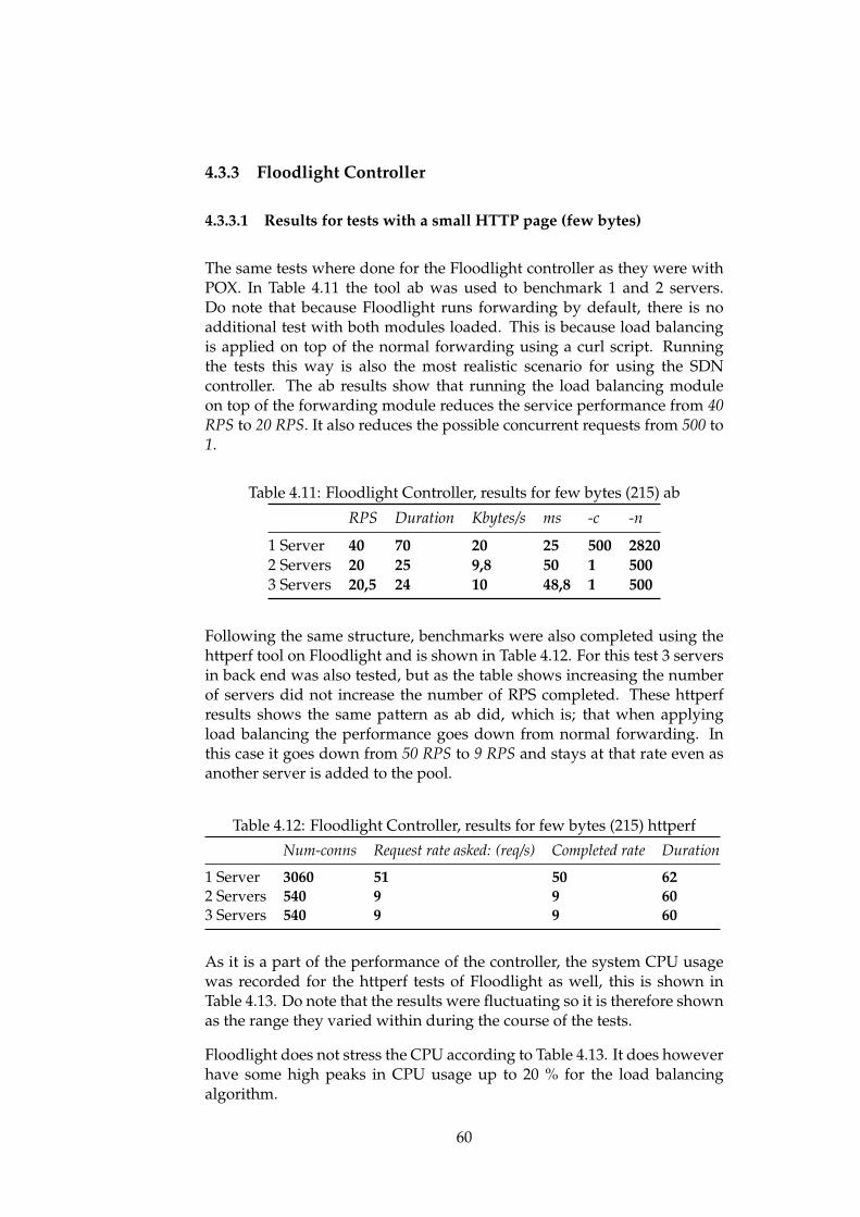
4.3.3 Floodlight Controller

4.3.3.1 Results for tests with a small HTTP page (few bytes)

The same tests where done for the Floodlight controller as they were withPOX. In Table 4.11 the tool ab was used to benchmark 1 and 2 servers.Do note that because Floodlight runs forwarding by default, there is noadditional test with both modules loaded. This is because load balancingis applied on top of the normal forwarding using a curl script. Runningthe tests this way is also the most realistic scenario for using the SDNcontroller. The ab results show that running the load balancing moduleon top of the forwarding module reduces the service performance from 40RPS to 20 RPS. It also reduces the possible concurrent requests from 500 to1.

Table 4.11: Floodlight Controller, results for few bytes (215) ab


1 Server 40 70 20 25 500 28202 Servers 20 25 9,8 50 1 5003 Servers 20,5 24 10 48,8 1 500

Following the same structure, benchmarks were also completed using thehttperf tool on Floodlight and is shown in Table 4.12. For this test 3 serversin back end was also tested, but as the table shows increasing the numberof servers did not increase the number of RPS completed. These httperfresults shows the same pattern as ab did, which is; that when applyingload balancing the performance goes down from normal forwarding. Inthis case it goes down from 50 RPS to 9 RPS and stays at that rate even asanother server is added to the pool.

Table 4.12: Floodlight Controller, results for few bytes (215) httperf

Num-conns Request rate asked: (req/s) Completed rate Duration

1 Server 3060 51 50 622 Servers 540 9 9 603 Servers 540 9 9 60

As it is a part of the performance of the controller, the system CPU usagewas recorded for the httperf tests of Floodlight as well, this is shown inTable 4.13. Do note that the results were fluctuating so it is therefore shownas the range they varied within during the course of the tests.

Floodlight does not stress the CPU according to Table 4.13. It does howeverhave some high peaks in CPU usage up to 20 % for the load balancingalgorithm.

60

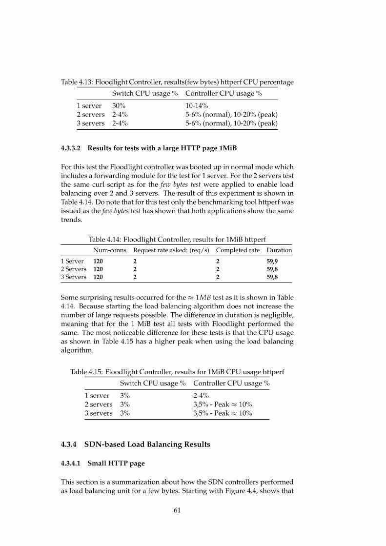
Table 4.13: Floodlight Controller, results(few bytes) httperf CPU percentage


1 server 30% 10-14%2 servers 2-4% 5-6% (normal), 10-20% (peak)3 servers 2-4% 5-6% (normal), 10-20% (peak)

4.3.3.2 Results for tests with a large HTTP page 1MiB

For this test the Floodlight controller was booted up in normal mode whichincludes a forwarding module for the test for 1 server. For the 2 servers testthe same curl script as for the few bytes test were applied to enable loadbalancing over 2 and 3 servers. The result of this experiment is shown inTable 4.14. Do note that for this test only the benchmarking tool httperf wasissued as the few bytes test has shown that both applications show the sametrends.

Table 4.14: Floodlight Controller, results for 1MiB httperfNum-conns Request rate asked: (req/s) Completed rate Duration

1 Server 120 2 2 59,92 Servers 120 2 2 59,83 Servers 120 2 2 59,8

Some surprising results occurred for the ≈ 1MB test as it is shown in Table4.14. Because starting the load balancing algorithm does not increase thenumber of large requests possible. The difference in duration is negligible,meaning that for the 1 MiB test all tests with Floodlight performed thesame. The most noticeable difference for these tests is that the CPU usageas shown in Table 4.15 has a higher peak when using the load balancingalgorithm.

Table 4.15: Floodlight Controller, results for 1MiB CPU usage httperf


1 server 3% 2-4%2 servers 3% 3,5% - Peak ≈ 10%3 servers 3% 3,5% - Peak ≈ 10%

4.3.4 SDN-based Load Balancing Results

4.3.4.1 Small HTTP page

This section is a summarization about how the SDN controllers performedas load balancing unit for a few bytes. Starting with Figure 4.4, shows that

61

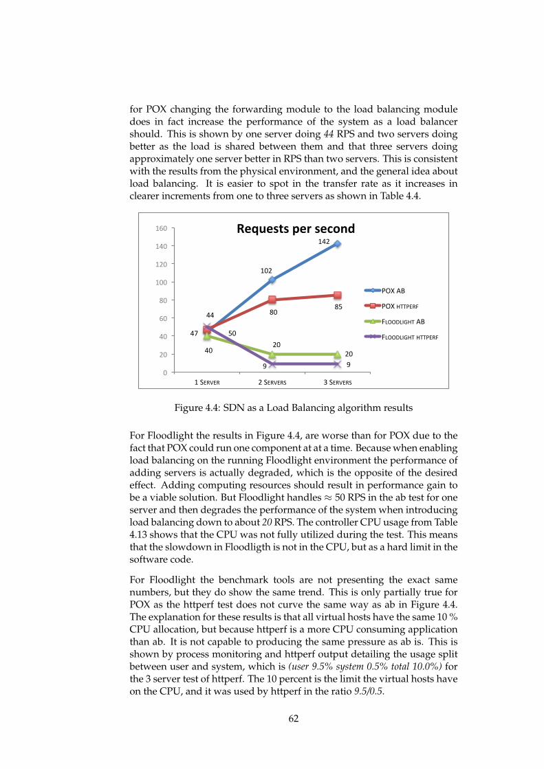
for POX changing the forwarding module to the load balancing moduledoes in fact increase the performance of the system as a load balancershould. This is shown by one server doing 44 RPS and two servers doingbetter as the load is shared between them and that three servers doingapproximately one server better in RPS than two servers. This is consistentwith the results from the physical environment, and the general idea aboutload balancing. It is easier to spot in the transfer rate as it increases inclearer increments from one to three servers as shown in Table 4.4.

44

102

142

47

80 85

40 20

20

50

9 9 0

20

40

60

80

100

120

140

160

1 SERVER 2 SERVERS 3 SERVERS

Requests per second

POX AB

POX HTTPERF

FLOODLIGHT AB

FLOODLIGHT HTTPERF

Figure 4.4: SDN as a Load Balancing algorithm results

For Floodlight the results in Figure 4.4, are worse than for POX due to thefact that POX could run one component at at a time. Because when enablingload balancing on the running Floodlight environment the performance ofadding servers is actually degraded, which is the opposite of the desiredeffect. Adding computing resources should result in performance gain tobe a viable solution. But Floodlight handles ≈ 50 RPS in the ab test for oneserver and then degrades the performance of the system when introducingload balancing down to about 20 RPS. The controller CPU usage from Table4.13 shows that the CPU was not fully utilized during the test. This meansthat the slowdown in Floodligth is not in the CPU, but as a hard limit in thesoftware code.

For Floodlight the benchmark tools are not presenting the exact samenumbers, but they do show the same trend. This is only partially true forPOX as the httperf test does not curve the same way as ab in Figure 4.4.The explanation for these results is that all virtual hosts have the same 10 %CPU allocation, but because httperf is a more CPU consuming applicationthan ab. It is not capable to producing the same pressure as ab is. This isshown by process monitoring and httperf output detailing the usage splitbetween user and system, which is (user 9.5% system 0.5% total 10.0%) forthe 3 server test of httperf. The 10 percent is the limit the virtual hosts haveon the CPU, and it was used by httperf in the ratio 9.5/0.5.

62

4.3.4.2 Large/intensive HTTP requests

This section is a summarization about how the SDN controllers performedas load balancing unit for a lager load of ≈ 1MB. What is clear fromFigure 4.5 is that as the servers increase, so does the performance whileusing the POX controller. This is however not a strictly fair comparisonas Floodlight must run both modules, but there is no way of disablingthe forwarding module in Floodlight as it is a dependency for the loadbalancing module.

0

1

2

3

4

5

6

7

1 Server 2 Servers 3 Servers

Requests per second

POX

Floodlight

Figure 4.5: SDN as a Load Balancing algorithm results for large load

4.3.5 Proactive POX load balancing

As the previous results involved benchmarking of reactive solutions,this section covers the development of a proof-of-concept solution, forproactive POX load balancing for performance benchmarking purposes.As version lower than 1.5 of OpenFlow does not support port matchingon TCP flags (e.g. SYN, FIN, and RST) the proactive solution can’t accountfor the status for a TCP connection (OpenFlow, 2014). This is also the casefor the reactive solutions that have been tested. This makes connectionmigration from one server to another harder, but it is not considered at thisstage.

The solution uses the arp_responder and forwarding.l2_learning componentfrom POX to provide what would be a realistic environment where normalforwarding and load balancing is enabled. The forwarding componentcomes bundled with the latest version of POX, but arp_responder has to bemanually installed from source (J. McCauley, 2013) as it is not included inlatest release of Mininet. This is done by coping the component into theext folder in the pox directory. The component file created is shown in

63

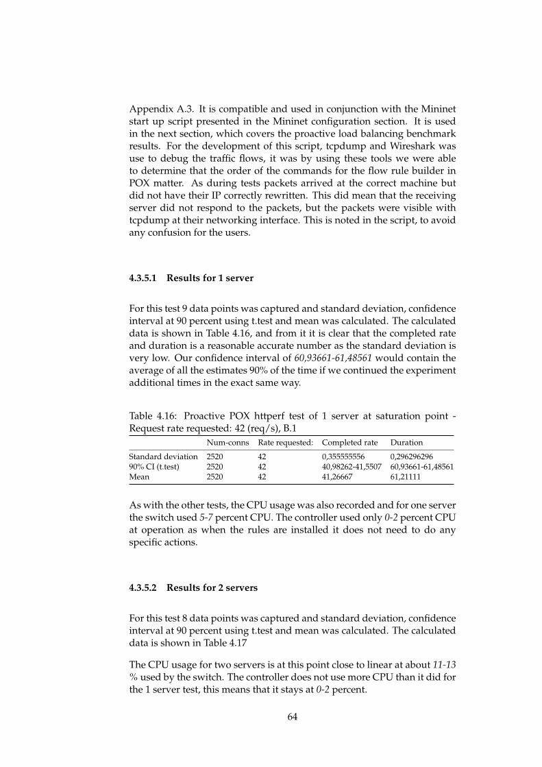
Appendix A.3. It is compatible and used in conjunction with the Mininetstart up script presented in the Mininet configuration section. It is usedin the next section, which covers the proactive load balancing benchmarkresults. For the development of this script, tcpdump and Wireshark wasuse to debug the traffic flows, it was by using these tools we were ableto determine that the order of the commands for the flow rule builder inPOX matter. As during tests packets arrived at the correct machine butdid not have their IP correctly rewritten. This did mean that the receivingserver did not respond to the packets, but the packets were visible withtcpdump at their networking interface. This is noted in the script, to avoidany confusion for the users.

4.3.5.1 Results for 1 server

For this test 9 data points was captured and standard deviation, confidenceinterval at 90 percent using t.test and mean was calculated. The calculateddata is shown in Table 4.16, and from it it is clear that the completed rateand duration is a reasonable accurate number as the standard deviation isvery low. Our confidence interval of 60,93661-61,48561 would contain theaverage of all the estimates 90% of the time if we continued the experimentadditional times in the exact same way.

Table 4.16: Proactive POX httperf test of 1 server at saturation point -Request rate requested: 42 (req/s), B.1

Num-conns Rate requested: Completed rate Duration

Standard deviation 2520 42 0,355555556 0,29629629690% CI (t.test) 2520 42 40,98262-41,5507 60,93661-61,48561Mean 2520 42 41,26667 61,21111

As with the other tests, the CPU usage was also recorded and for one serverthe switch used 5-7 percent CPU. The controller used only 0-2 percent CPUat operation as when the rules are installed it does not need to do anyspecific actions.

4.3.5.2 Results for 2 servers

For this test 8 data points was captured and standard deviation, confidenceinterval at 90 percent using t.test and mean was calculated. The calculateddata is shown in Table 4.17

The CPU usage for two servers is at this point close to linear at about 11-13% used by the switch. The controller does not use more CPU than it did forthe 1 server test, this means that it stays at 0-2 percent.

64

Table 4.17: Proactive POX httperf test of 2 servers at saturation point -Request rate requested: 84 (42x2) (req/s), B.2


Standard deviation 5040(2520x2) 84 (42x2) 0,34375 0,08062222290% CI interval,(t.test) 5040(2520x2) 84 (42x2) 82,99482-83,75518 60,23185-60,31815Mean 5040(2520x2) 84 (42x2) 83,375 61,21111

4.3.5.3 Results for 1 and 2 servers (1 MiB)

The test with 1 MiB is presented in Table 4.18. Here the controller has a lowCPU usage at about 0-2 percent. As for the switch it uses ≈ 2% for 1 serverand ≈ 4% for 2 servers. This means that the switch CPU usage scales withthe RPS completed.

Table 4.18: Proactive POX httperf test of servers at saturation point for 1MiB


1 Server 120 2 2 60,032 Servers 240(120x2) 4(2x2) 4 59,98

4.3.5.4 Proactive solution

The proactive solution where rules are installed into the switch before apacket arrives gives a linear curve for this test scenario as shown in Figure4.6. Because this solution does load balancing based on source IP for onevirtual IP (VIP), there must be on client for each server. This also meansas long as the CPU usage of the system is not at maximum, it is possible tocontinue to add new servers and clients to get more RPS total. One notationis that the CPU usage of the controller stays at 1% as it does not need toactively interact with the switches.

As for the test with bigger load, it behaves in the same fashion as for thesmall HTTP requests, because increasing servers does linearly increase theRPS possible.

4.4 Solutions comparison

As we know that the proactive solution scales linearly, the 3 server resultsfor proactive can be calculated, and all httperf results can be insertedinto a graph. This has been done in Figure 4.7 and it shows how theperformance of the proactive and reactive solutions. What is clear is thatnone of these setups are without their drawbacks. For instance does theproactive solution provide best performance. However, it will require

65

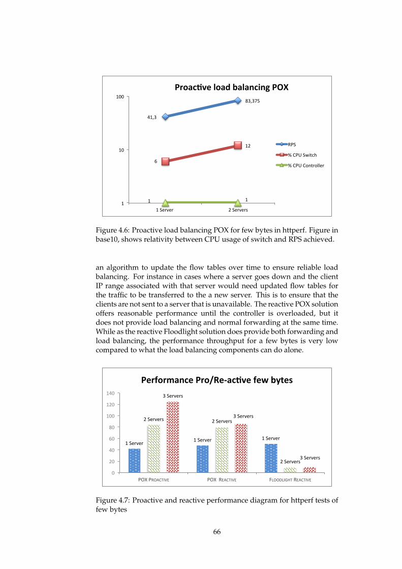
41,3

83,375

6

12

1 1 1

10

100

1 Server 2 Servers

Proac&ve load balancing POX

RPS

% CPU Switch

% CPU Controller

Figure 4.6: Proactive load balancing POX for few bytes in httperf. Figure inbase10, shows relativity between CPU usage of switch and RPS achieved.

an algorithm to update the flow tables over time to ensure reliable loadbalancing. For instance in cases where a server goes down and the clientIP range associated with that server would need updated flow tables forthe traffic to be transferred to the a new server. This is to ensure that theclients are not sent to a server that is unavailable. The reactive POX solutionoffers reasonable performance until the controller is overloaded, but itdoes not provide load balancing and normal forwarding at the same time.While as the reactive Floodlight solution does provide both forwarding andload balancing, the performance throughput for a few bytes is very lowcompared to what the load balancing components can do alone.

1 Server 1 Server 1 Server

2 Servers 2 Servers

2 Servers

3 Servers

3 Servers

3 Servers

0

20

40

60

80

100

120

140

POX PROACTIVE POX REACTIVE FLOODLIGHT REACTIVE

Performance Pro/Re-‐ac.ve few bytes

Figure 4.7: Proactive and reactive performance diagram for httperf tests offew bytes

66

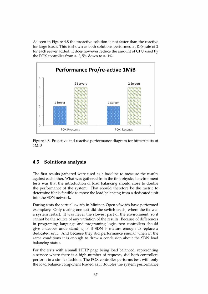
As seen in Figure 4.8 the proactive solution is not faster than the reactivefor large loads. This is shown as both solutions performed at RPS rate of 2for each server added. It does however reduce the amount of CPU used bythe POX controller from ≈ 3, 5% down to ≈ 1%.

1 Server 1 Server

2 Servers 2 Servers

0

1

2

3

4

5

POX PROACTIVE POX REACTIVE

Performance Pro/re-‐ac-ve 1MiB

Figure 4.8: Proactive and reactive performance diagram for httperf tests of1MiB

4.5 Solutions analysis

The first results gathered were used as a baseline to measure the resultsagainst each other. What was gathered from the first physical environmenttests was that the introduction of load balancing should close to doublethe performance of the system. That should therefore be the metric todetermine if it is feasible to move the load balancing from a dedicated unitinto the SDN network.

During tests the virtual switch in Mininet, Open vSwitch have performedexemplary. Only during one test did the switch crash, where the fix wasa system restart. It was never the slowest part of the environment, so itcannot be the source of any variation of the results. Because of differencesin programing language and programing logic, two controllers shouldgive a deeper understanding of if SDN is mature enough to replace adedicated unit. And because they did performance similar when in thesame conditions it is enough to draw a conclusion about the SDN loadbalancing status.

For the tests with a small HTTP page being load balanced, representinga service where there is a high number of requests, did both controllersperform in a similar fashion. The POX controller performs best with onlythe load balance component loaded as it doubles the system performance

67

from 1 to 2 servers as load balancer should. What is disappointing howeveris that when POX is started in a realistic scenario with both forwarding andload balancing it can not sustain a feasible RPS or kbytes/s throughput forboth the httperf and ab test. What is the most surprising about this, is that itis not a system resource limitation as it only uses a few percent of the CPU,so the limit here lies within the programing itself. This means that it won’tbe a viable solution in a full-scale environment as adding more resourceswould not solve this limitation of the setup. The odds are further stackedagainst SDN load balancing as the Floodlight setup encounters the samelimit with both components loaded as POX did. That unfortunately meansthat the slight performance advantage it has is negligible as that is just forthe baseline results without load balancing.

The results for the scenario with large file transfers are where the controllersshow their clear differences. Both components are loaded on bothcontrollers for this scenario and in these results POX is actually functioningas a load balancer where as Floodlight is not. Because POX has a linearexpansion curve as shown in Figure 4.5, however for Floodlight in thisfigure the line is flat. The line is flat because Floodlight does not manage toincrease the RPS for the large file transfers scenario.

This means that, if choosing between POX and Floodlight that POX is theobvious choice for large file transfer load balancing. It however also provesthat none of the tested SDN controllers should be used as a replacementfor a dedicated hardware load balancer for small file transfers/requests.With that in mind it, from Figure 4.7 it seems feasible to run a proactiveload balancer using the POX controller. Because doing so, the only reallimitation is in the switches themselves and not in the controller. Itwould however mean that for it to be used in a production environment,that it were more advanced so it could handle a larger variation ofincoming clients and automatically distributing the source IP ranges overthe available back-end servers based on availability.

If the traffic that needs to be load balanced is for large file transfers orcomputing heavy requests, so that the amount of concurrent requests arelower than for instance a typical web page with a high number of users itseems reasonable to run SDN load balancing but only as long as there is noforwarding needed. If the network needs a forwarding controller as well,as a typical production network does, using SDN load balancing for largerequests is not feasible. As in terms of scalability of the solutions, doesthe controllers use the most CPU. This is because the clients and serversare limited, but the controller application could use as much CPU as thevirtual environment had available. This means that for a full-scale solutionif the controller needs to work in a reactive mode, the network throughputis solely dependent on the speed of the controller.

68

Chapter 5

Discussion and Future Work

5.1 Discussion and Conclusion

The HTTP tests used for benchmarking have produced valid and intendeddata. The results are valid because they show clear patterns of thetested solutions and from the results themselves there were no surprises.Although, in what the results told when analysed was surprising withregards to the controllers using multiple components. Some comparabledata is hard to find, as the BIG-IP does not have a HTTP load balancingrate listed in its hardware specification sheet. This is also true for thevirtual environment, as the load balancing algorithms have not been testedin this type of setup. To reproduce the same results for another researcherwould be trivial for the virtual environment, as it only uses free to use tools.However, for the physical environment a BIG-IP LTM device would be anexpensive hardware to acquire for the same test.

5.1.1 Network topology

All the papers explored in the related work section, that had some successwith SDN-based balancing tested unstructured network topologies, wherethere is no clear source of client requests. There were, however no papersthat tested a scenario as if SDN could replace a dedicated hardware loadbalancer in a structured or random network. However, this thesis onlylooks into a structured network, because that is the main configuration fora dedicated load balancing unit.

5.1.2 Feasibility cases for SDN

This thesis provides predictions for the feasibility of replacing a LTM unitas the BIG-IP with an SDN-based solution. There are three cases that it ispossible to make predictions about:

69

1. Small requests

(a) Requests that have short processing time or small packets beingsent with a high amount of users.

2. Big requests

(a) Requests that uses a lot of bandwidth, like a large file trans-fer.

3. CPU intensive requests

(a) Requests that are computationally heavy, e.g that the back-endservers use a long time for processing so that the amount ofusers are lower than for small packets with a high amount ofusers.

The two last cases, 2 and 3 are possible to merge as they are similar in theway that the controller only needs installed a few flow rules. What wasshown in the analysis Section 4.5 with regards to these cases is that SDN-based load balancing is probably not in the near future going to replacea dedicated unit for case 1. Because both tested solutions did not handlea high RPS satisfactorily, and would clearly have some limitations withrespect to system resources. This limitation is based on the fact that thededicated unit has a higher CPU to RPS ratio even just for forwarding,which was what the controllers supported for best performance.

With regards to case 2 and 3 they are much more promising as Section4.5 outlined. This is because the CPU usage is much lower, and whenonly running a load balancing algorithm their speed is linearly increasingas long as there is available CPU. However, though the SDN controllershave a hard limit, the programing limitations are their biggest obstacle forbecoming feasible. This hard limit in software was a big surprise as someincompatibility or high CPU usage was to be expected, but not such asbreakdown as the controllers did with both modules loaded.

5.1.3 Load Balancing algorithms

For the most promising controller POX, the load balancing algorithmsupplied picks servers in a random fashion. This cause more unpredictableresults as it may easier overload one of the backend servers. This resultedin that a lot of the tests had to be remeasured to ensure that the result wasstable. In contrast to the BIG-IP that does not have a random algorithm,it did prove to give more stable results as the algorithm round robindivides the load better. The other controller Floodlight, also providesload balancing after the round robin principle. However, as the controllerstruggles with a software limitation it does not impact the measured resultsin a positive way.

70

5.1.4 Mininet bug, implications on recorded data

A high level Mininet CLI script was developed to automate the benchmark-ing process. Unfortunately, an undocumented python/bash bug stop theservers after a given amount of console output. However, when servers arestarted with h3.cmd(’http-server -p 80 &’) instead of manually typed into theXTerm console the performance suffers. Starting the servers like that re-sulted in them stopping because of the output buffer being filled up. Thatis why all servers were initiated manually by typing http-server -p 80 intothe XTerm CLI. This is however a much more tedious and slower processas the environment is reset between each test for a clean test each time. Thebiggest impact of this bug for this thesis is that originally it was intended touse the Mininet high-level API function for this automated sequence.

1: Boot network. 2: Start services. 3: Do performance test. 4: Logdata.

However as the solution to this limitation were discovered three daysbefore the delivery date by consulting the Mininet development team,the script was not used to conduct the tests. But most of the script isalready developed and included in this thesis, some reconfiguration wouldhowever be needed for complete automation as it was not completedbecause of this error. If the functionality had worked, collecting more data-points (30+) for all tests would have been feasible. It does not howeverhave a big impact in the value of the data as all collected data showclear tendencies. As for further tests, the variance in data is dependenton the host operating system. However, by using the provided Mininetscripts all data recorded on other systems will show the same graphs andpercentage differences, with the baseline results varies with the maximumprocessing power of the host operating system. Using this script is strictlyrecommended, as it was a mistake not to consult the development teamearlier to overcome this limitation.

5.1.5 MiB instead of MB

When the 1 and 2 MiB test files where created, it was the intention to create1 MB files for the simple denomination. However the inputted multiplierwas 1024 instead of 1000 for the dd command, resulting in 1 and 2 Mebibyte(MiB) size files. This error was not uncovered until multiple experimentshad been conducted, and was therefore not corrected. The only implicationof this however, is the denominator for the tests as the byte difference doesnot make any impact on the test as both controllers were tested using thesame MiB files.

71

5.1.6 Problem statement

The main idea of the problem statement of this thesis was to find out ifSDN-based load balancing could in some way replace a dedicated LTMunit. For this it also needed to configure an LTM device to have somethingto compare the SDN solutions to. This did however require time whichif not needed could have been spent on benchmarking additional SDNcontrollers’ load balancing algorithms.

5.1.6.1 Was the problem statement answered?

1. How to setup a load balancing algorithm in SDN in order to achieveperformance comparable to a physical load balancer.

(a) Setting up load balancing for SDN was covered in approachsections 3.4.1 and 3.4.2, they were then tested in Chapter 4, asthere was no way of knowing beforehand how the differentcontrollers performed. Different approaches were tested butclear limitations were discovered in the analysis in Section 4.5.In this section, software limitations were discovered that didnot allow for a setup that could compare with the performanceand switching capabilities of the BIG-IP 1600 series LTM. Theresults also show that the controllers’ real limitation is theirsystem CPU. So if the controller resources can scale up to an LTMdevice in processing power, solving the software limitationswould lead to a comparable SDN-based load balancing solution.Unfortunately, writing a better reactive algorithm than whatthe developers of POX and Floodlight have produced seemedunachievable in the allocated time-frame.

2. Study, setup and run a physical load balancer (BIG-IP-1600 series).

(a) The provided load balancer from Jottacloud came pre-configuredwith unknown system passwords. Studying of service manualsand reconfiguring the device to interact with the Linux serversrevealed that the device would only interact with VLAN taggedpackets in the approach Section 3.2.1. As regard to the ap-proach in retrospect, evaluating more controllers performancemeasured against each other instead of using a lot of time on con-figuring the physical environment would have been more bene-ficial for the SDN research field. This is because the results gath-ered from the physical environment don’t have a physical coun-terpart SDN-based device to be compared too. The results how-ever and the process of obtaining them are useful as the methodscould be applied to the understanding and benchmarking of thevirtual systems.

72

3. Compare an SDN load balancer to a hardware load balancer in terms ofscalability and performance.

(a) Performance:

i. In Section 4.3 a performance graph for the physical envi-ronment was produced as a result of multiple performancetests. This shows a linear curve for using load balancing andthat the CPU is the limiting factor. The same tests wheretherefore conducted on the virtual environment with theproperties of the physical environment as a reference point.Analyses of these results in Section 4.5n shows that in somecases the SDN controllers may also achieve a linear perfor-mance curve similar to the physical unit.

(b) Scalability:

i. In terms of scalability, the 4.5 section shows that scaling ofSDN load balancing is dependent on the controller. Thismeans that the SDN-based solutions would scale as long asthe controller could get more CPU power. This howeverseems more likely for the POX controller, as the modulesare independent. Meaning that it is possible to turn offorwarding in POX, but if forwarding is turned off inFloodlight, the load balancing module does not work.

5.2 Recommendations for Future Work

This thesis ended up with good data for the physical environment andfor two SDN-controllers in an automated Mininet environment. This alsoresulted in some predictions about the feasibility of an SDN-based loadbalancing, but as the SDN topic is wast and fast growing, covering allcases were not possible. However, based on the collated information someinsight into good opportunities for further work in terms of another thesis,research papers or small projects is presented below:

As of now the tested controllers POX and Floodlight does not provide thesame ease of operation as the BIG-IP delivers. Although the tests showthat they can deliver similar performance in some scenarios. We cannotconclusively say that SDN can replace HTTP load balancing for smallrequests. Using a proactive setup the approach is possible and promisingbut it is probably not a wanted scenario for most users. For future worktesting commercial controllers in the same scenarios could yield results,but are most likely prone to the same limits as the tested controllers. Forconclusive results however, rerunning the tests on a physical OpenFlowenabled switch in a full-scale environment should be conducted in order todetermine if the controller CPU load actually does impact the performance

73

as heavily as in the virtual environment.

From the results gathered, it is clear that processing power is the mainlimitation of an SDN-based load balancing. This means that expandingthe work into more powerful controller applications would be a goodresearch field. An example of this is an SDN controller that can run in acluster for more processing power. This could be made possible with theHelium OpenDaylight SDN cluster and a OpenFlow switch that supportsthe OpenFlow 1.3.2 specification OFPCR_ROLE_EQUAL, which can setmultiple controllers to control one switch. Another possibility is dividingthe OpenFlow switch into different slices for different network traffic, likeone slice for TCP (HTTP) and the other for IP switching with the FlowVisorsoftware. This may possibly open up opportunities to either divide theroles of the controllers so that only one controller handles load balancing orincrease the total throughput for the controller’s load balancing algorithm.Either solution is an interesting topic for future research, as they both maymake SDN load balancing viable.

There are many SDN controllers to chose from that supports loadbalancing, and while some are commercial grade like Vyatta, not all are.For instance is the OpenDaylight controller not commercial, and it comesbundled with a load balancing service. This means that it is possible to testeven more controllers to help determining if some controllers can replace adedicated unit. However, does Mininet not provide a direct comparisonbetween a physical unit as it a virtualization. So to fully compare theSDN controllers to a physical unit; using an OpenFlow enables switchwould enable that comparison. Unfortunately it was not an option duringthis thesis but it could be for other future projects. This means that bothapproaches are good future projects and if exploring additional controllersin Mininet, the high-level CLI script that has been developed in this thesis,is a good tool for benchmarking as only small changes would be requiredto support other controllers.

74

Bibliography

Armor, C. (n.d.). F5-big-ltm-1600. Retrieved February 3, 2015, from http ://www.corporatearmor.com/

Asai, H., Fukuda, K., & Esaki, H. (2011). Traffic causality graphs: profilingnetwork applications through temporal and spatial causality of flows.In Proceedings of the 23rd international teletraffic congress (pp. 95–102).ITC ’11. San Francisco, California: International Teletraffic Congress.Retrieved from http://dl.acm.org/citation.cfm?id=2043468.2043484

Azodolmolky, S. (2013). Software defined networking with openflow. PACKT.Chua, R. (2012). Nox pox and controllers galore murphy mccauley

interview. Retrieved January 29, 2015, from https://www.sdxcentral.com/articles/interview/noxpox- controllers- murphy- mccauley/2012/09/

CISCO. (2015). What is a network switch vs. a router? Retrieved January26, 2015, from http : / / www. cisco . com / cisco / web / solutions /small_business/resource_center/articles/connect_employees_and_offices/what_is_a_network_switch/index.html

Cole, A. (2013). The end of the road for the vlan? not quite. RetrievedFebruary 2, 2015, from http : / / www. enterprisenetworkingplanet .com/datacenter/datacenter- blog/end- of- the- road- for- the- vlan.html

Contemporary Control Systems, I. (2002). Hubs versus switches—understandthe tradeoffs. theEXTENSION, 3. Retrieved February 10, 2015, fromhttp://www.ccontrols.com/pdf/Extv3n3.pdf

Edelman, J. (2013). Are there alternatives to the openflow protocol?Retrieved January 30, 2015, from http://searchsdn.techtarget.com/answer/Are-there-alternatives-to-the-OpenFlow-protocol

F5. (n.d.). Platform guide: 1600. Retrieved February 3, 2015, from https :/ / support . f5 . com / content / kb / en - us / products / big - ip _ ltm /manuals/product/pg_1600/_jcr_content/pdfAttach/download/file.res/Platform_Guide__1600.pdf

F5. (2015). Load balancer. Retrieved February 3, 2015, from https : / / f5 .com/glossary/load-balancer

Feamster, N., Rexford, J., & Zegura, E. (2013, December). The road to sdn.Queue, 11(12), 20:20–20:40. doi:10.1145/2559899.2560327

Floodlight, P. (2015). Floodlight is an open sdn controller. RetrievedFebruary 21, 2015, from http : / / www . projectfloodlight . org /floodlight/

75

http://www.corporatearmor.com/

http://www.corporatearmor.com/

http://dl.acm.org/citation.cfm?id=2043468.2043484

https://www.sdxcentral.com/articles/interview/nox-pox-controllers-murphy-mccauley/2012/09/



http://www.cisco.com/cisco/web/solutions/small_business/resource_center/articles/connect_employees_and_offices/what_is_a_network_switch/index.html



http://www.enterprisenetworkingplanet.com/datacenter/datacenter-blog/end-of-the-road-for-the-vlan.html



http://www.ccontrols.com/pdf/Extv3n3.pdf

http://searchsdn.techtarget.com/answer/Are-there-alternatives-to-the-OpenFlow-protocol

http://searchsdn.techtarget.com/answer/Are-there-alternatives-to-the-OpenFlow-protocol

https://support.f5.com/content/kb/en-us/products/big-ip_ltm/manuals/product/pg_1600/_jcr_content/pdfAttach/download/file.res/Platform_Guide__1600.pdf




https://f5.com/glossary/load-balancer

https://f5.com/glossary/load-balancer

http://dx.doi.org/10.1145/2559899.2560327

http://www.projectfloodlight.org/floodlight/

http://www.projectfloodlight.org/floodlight/

Ghaffarinejad, A. & Syrotiuk, V. (2014, March). Load balancing in acampus network using software defined networking. In Researchand educational experiment workshop (gree), 2014 third geni (pp. 75–76).doi:10.1109/GREE.2014.9

Handigol, N., Seetharaman, S., Flajslik, M., Johari, R., & McKeown, N.(2010, November). Aster*x: load-balancing as a network primitive.9th GENI Engineering Conference (Plenary).

Handigol, N., Seetharaman, S., Flajslik, M., McKeown, N., & Johari,R. (2009). Plug-n-serve: load-balancing web traffic using openflow.Sigcomm Demonstration.

Iperf. (2014). What is iperf? Retrieved January 28, 2015, from https://iperf.fr/

Jesse. (2015). Bip-ip 1600 vlan bridge performance degradation. RetrievedMarch 8, 2015, from https://devcentral.f5.com/questions/bip- ip-1600-vlan-bridge-performance-degradation

Johnson, S. (2012). A primer on northbound apis: their role in a software-defined network. Retrieved January 30, 2015, from http://searchsdn.techtarget.com/feature/A-primer-on-northbound-APIs-Their-role-in-a-software-defined-network

Laboratories, H.-P. R. (n.d.-a). 2 an example of using httperf. Retrieved fromhttp://www.hpl.hp.com/research/linux/httperf/wisp98/html/doc003.html

Laboratories, H.-P. R. (n.d.-b). Httperf(1) - linux man page. Retrieved fromhttp://linux.die.net/man/1/httperf

Limoncelli, T. A. (2012, June). Openflow: a radical new idea in networking.Queue, 10(6), 40:40–40:46. doi:10.1145/2246036.2305856

McCauley, J. (2013). Arp responder.py. Retrieved May 4, 2015, from https://github.com/CPqD/RouteFlow/blob/master/pox/pox/misc/arp_responder.py

McCauley, M. & Al-Shabibi, A. (2014). Pox wiki. Retrieved February 7, 2015,from https://openflow.stanford.edu/display/ONL/POX+Wiki

McKeown, N. (2011). How sdn will shape networking. Retrieved February9, 2015, from https://www.youtube.com/watch?v=c9-K5O_qYgA

Morin, J. (2014). Conflicting trends part 2: sdn and converged in-frastructure. Retrieved January 26, 2015, from http : / / www .extremenetworks . com / conflicting - trends - part - 2 - sdn - and -converged-infrastructure

NOXRepo.org. (2015). About pox. Retrieved January 29, 2015, from http://www.noxrepo.org/pox/about-pox/

Oliver, B. (2014). Pica8: first to adopt openflow 1.4; why isn’t anyone else?Retrieved February 7, 2015, from http : / / www. tomsitpro . com /articles/pica8-openflow-1.4-sdn-switches,1-1927.html

open networking foundation. (2015). Software-defined networking (sdn)definition. Retrieved January 30, 2015, from https : / / www .opennetworking.org/sdn-resources/sdn-definition

OpenFlow. (2009). Openflow switch specification. Retrieved February 4,2015, from http : / / archive . openflow. org / documents / openflow -spec-v1.0.0.pdf

76

http://dx.doi.org/10.1109/GREE.2014.9

https://iperf.fr/

https://iperf.fr/

https://devcentral.f5.com/questions/bip-ip-1600-vlan-bridge-performance-degradation

https://devcentral.f5.com/questions/bip-ip-1600-vlan-bridge-performance-degradation

http://searchsdn.techtarget.com/feature/A-primer-on-northbound-APIs-Their-role-in-a-software-defined-network



http://www.hpl.hp.com/research/linux/httperf/wisp98/html/doc003.html

http://www.hpl.hp.com/research/linux/httperf/wisp98/html/doc003.html

http://linux.die.net/man/1/httperf

http://dx.doi.org/10.1145/2246036.2305856

https://github.com/CPqD/RouteFlow/blob/master/pox/pox/misc/arp_responder.py



https://openflow.stanford.edu/display/ONL/POX+Wiki

https://www.youtube.com/watch?v=c9-K5O_qYgA

http://www.extremenetworks.com/conflicting-trends-part-2-sdn-and-converged-infrastructure



http://www.noxrepo.org/pox/about-pox/

http://www.noxrepo.org/pox/about-pox/

http://www.tomsitpro.com/articles/pica8-openflow-1.4-sdn-switches,1-1927.html

http://www.tomsitpro.com/articles/pica8-openflow-1.4-sdn-switches,1-1927.html

https://www.opennetworking.org/sdn-resources/sdn-definition

https://www.opennetworking.org/sdn-resources/sdn-definition

http://archive.openflow.org/documents/openflow-spec-v1.0.0.pdf

http://archive.openflow.org/documents/openflow-spec-v1.0.0.pdf

OpenFlow. (2013). Openflow switch specification 1.3.3. Retrieved February4, 2015, from https://www.opennetworking.org/images/stories/downloads/sdn-resources/onf-specifications/openflow/openflow-spec-v1.3.3.pdf

OpenFlow. (2014). Openflow switch specification 1.5. Retrieved February4, 2015, from https://www.opennetworking.org/images/stories/downloads/sdn-resources/onf-specifications/openflow/openflow-switch-v1.5.0.noipr.pdf

Pacchiano, R. (2006). The difference between hubs, switches and routers.Retrieved January 27, 2015, from http : / / www. webopedia . com /DidYouKnow/Hardware_Software/router_switch_hub.asp

Phaal, P. (2013). Sdn and large flows. Retrieved February 3, 2015, from http://blog.sflow.com/2013/02/sdn-and-large-flows.html

Pronschinske, M. (2013). Controllers q&a: nox/pox , trema , beacon ,floodlight , routeflow. Retrieved January 26, 2015, from http : / /architects.dzone.com/articles/controllers-qa-noxpox-trema

Richard Wang, J. R., Dana Butnariu. (2011). Openflow-based server loadbalancing gone wild. Princeton University.

Rouse, M. (2007). Hardware load-balancing device (hld). Retrieved Febru-ary 3, 2015, from http : / / searchnetworking . techtarget . com /definition/hardware-load-balancing-device

Salisbury, B. (2012). Tcams and openflow – what every sdn practitionermust know. Retrieved February 7, 2015, from https : / / www .sdxcentral . com / articles / contributed / sdn - openflow - tcam - need -to-know/2012/07/

Team, M. (2014). Introduction to mininet. Retrieved February 23, 2015, fromhttps : / / github . com / mininet / mininet / wiki / Introduction - to -Mininet

Team, M. (2015). Mininet overview. Retrieved January 28, 2015, from http://mininet.org/overview/

Uppal, H. & Brandon, D. (n.d.). Openflow based load balancing. Universityof Washington - Project Report CSE561: Networking. RetrievedFebruary 11, 2015, from http://courses.cs.washington.edu/courses/cse561/10sp/project_files/cse561_openflow_project_report.pdf

Wang, K.-C. (2012). Load balancer. Retrieved February 22, 2015, from http:/ / www. openflowhub . org / display / floodlightcontroller / Load +Balancer

Wireshark. (2015). About. Retrieved January 28, 2015, from https://www.wireshark.org/about.html

Zito, P. (2013). What is the osi model. Retrieved January 27, 2015, from http://blog.buildingautomationmonthly.com/what-is-the-osi-model/

77

https://www.opennetworking.org/images/stories/downloads/sdn-resources/onf-specifications/openflow/openflow-spec-v1.3.3.pdf



https://www.opennetworking.org/images/stories/downloads/sdn-resources/onf-specifications/openflow/openflow-switch-v1.5.0.noipr.pdf



http://www.webopedia.com/DidYouKnow/Hardware_Software/router_switch_hub.asp

http://www.webopedia.com/DidYouKnow/Hardware_Software/router_switch_hub.asp

http://blog.sflow.com/2013/02/sdn-and-large-flows.html

http://blog.sflow.com/2013/02/sdn-and-large-flows.html

http://architects.dzone.com/articles/controllers-qa-noxpox-trema

http://architects.dzone.com/articles/controllers-qa-noxpox-trema

http://searchnetworking.techtarget.com/definition/hardware-load-balancing-device

http://searchnetworking.techtarget.com/definition/hardware-load-balancing-device

https://www.sdxcentral.com/articles/contributed/sdn-openflow-tcam-need-to-know/2012/07/



https://github.com/mininet/mininet/wiki/Introduction-to-Mininet

https://github.com/mininet/mininet/wiki/Introduction-to-Mininet

http://mininet.org/overview/

http://mininet.org/overview/

http://courses.cs.washington.edu/courses/cse561/10sp/project_files/cse561_openflow_project_report.pdf

http://courses.cs.washington.edu/courses/cse561/10sp/project_files/cse561_openflow_project_report.pdf

http://www.openflowhub.org/display/floodlightcontroller/Load+Balancer



https://www.wireshark.org/about.html

https://www.wireshark.org/about.html

http://blog.buildingautomationmonthly.com/what-is-the-osi-model/

http://blog.buildingautomationmonthly.com/what-is-the-osi-model/

Appendices

79

Appendix A

Mininet scripts

81

Listing A.1: POX Mininet

1 #!/ usr /bin /python23 from mininet . topo import Topo4 from mininet . net import Mininet5 from mininet . l i n k import TCLink6 from mininet . c l i import CLI7 from mininet . node import Con t r o l l e r89 from mininet . l i n k import TCIntf

10 from mininet . u t i l import custom , quietRun11 from mininet . node import CPULimitedHost12 from mininet . l og import setLogLevel , i n f o13141516 from fun c t o o l s import p a r t i a l17 import os1819 c l a s s SingleSwitchTopo (Topo) :20 " S ing l e ␣ switch ␣ connected ␣ to ␣n␣ hos t s . "21 de f bu i ld ( s e l f , n=2) :22 switch = s e l f . addSwitch ( ’ s1 ’ )23 f o r h in range (n) :24 host = s e l f . addHost ( ’ h%s ’ % (h + 1) )25 # Def ine network parameters l i k e de lay and

↪→ speed :26 s e l f . addLink ( host , switch , bw=820 , de lay = ’0.07

↪→ ms ’ , l o s s =0, use_htb=True )272829 c l a s s POXload ( Con t r o l l e r ) :30 " Cont r o l l e r ␣ c l a s s ␣ to ␣ s t a r t ␣ the ␣ c o n t r o l l e r "31 de f s t a r t ( s e l f ) :32 " Star t ␣POX␣component␣ o f ␣your␣ cho i s e : "33 s e l f . pox = ’%s/pox/pox . py ’ % os . env i ron [ ’HOME’ ]34 # Forwarding :35 #s e l f . cmd( s e l f . pox , ’ forward ing . l 2_learn ing &’ )36 # React ive Load balance :37 #s e l f . cmd( s e l f . pox , ’ misc . ip_loadbalancer −−ip

↪→ =10 .1 .2 . 3 −−s e r v e r s =1 0 . 0 . 0 . 2 , 1 0 . 0 . 0 . 3 , 1 0 . 0 . 0 . 4↪→ &’ )

38 # Proact ive Load balance :39 s e l f . cmd( s e l f . pox , ’ load arp_responder

↪→ − −10 .0 .0 .10=00 :00 :00 :00 :10 : f e forward ing .↪→ l 2_lea rn ing &’ )

40 de f stop ( s e l f ) :41 "Stop␣POX"42 s e l f . cmd( ’ k i l l %’ + s e l f . pox )4344 c o n t r o l l e r s = { ’ poxload ’ : POXload }4546 de f s t a r t s t u f f ( ) :47 # Def ine topology ( I .E number o f hos t s ) :48 topo = SingleSwitchTopo (n=4)49 # Def ine CPU l im i t s f o r hos t s :50 host = custom ( CPULimitedHost , sched=’ c f s ’ , period_us=10000 ,

↪→ cpu=.025 )51 # Def ine network :52 # autoSetMacs=True i s equ iva l en t to −−mac parameter53 net = Mininet ( topo=topo , l i n k=TCLink , c o n t r o l l e r=POXload( ’ c0

↪→ ’ , ip = ’127 . 0 . 0 . 1 ’ , port=6633 ) , host=host , autoSetMacs=↪→ True )

54 # Star t network :55 net . s t a r t ( )56 # Star t t e rmina l s57 #net . startTerms ( )

82

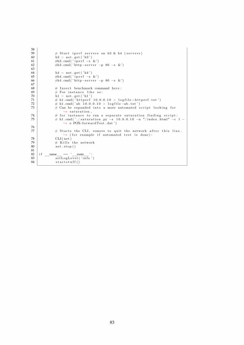
5859 # Star t i p e r f s e r v e r s on h3 & h4 ( s e r v e r s )60 h3 = net . get ( ’ h3 ’ )61 #h3 . cmd( ’ i p e r f −s & ’)62 #h3 . cmd( ’ http−s e r v e r −p 80 −s & ’)6364 h4 = net . get ( ’ h4 ’ )65 #h4 . cmd( ’ i p e r f −s & ’)66 #h4 . cmd( ’ http−s e r v e r −p 80 −s & ’)6768 # In s e r t benchmark command here :69 # For in s t anc e l i k e so :70 h1 = net . get ( ’ h1 ’ )71 # h1 . cmd( ’ h t t p e r f 1 0 . 0 . 0 . 1 0 > l o g f i l e −h t tp e r f . txt ’ )72 # h1 . cmd( ’ ab 1 0 . 0 . 0 . 1 0 > l o g f i l e −ab . txt ’ )73 # Can be expanded in to a more automated s c r i p t l ook ing f o r

↪→ sa tura t i on ,74 # fo r in s t ance to run a separa t e s a tu ra t i on f i nd i n g s c r i p t :75 # h1 . cmd ( ’ . / s a tu ra t i on . py −s 1 0 . 0 . 0 . 1 0 −u "/ index . html" −c 1 −

↪→ o POX−forwardTest . dat ’ )7677 # Sta r t s the CLI , remove to qu i t the network a f t e r t h i s l i n e .

↪→ ( f o r example i f automated t e s t i s done ) :78 CLI( net )79 # K i l l s the network80 net . stop ( )8182 i f __name__ == ’__main__’ :83 setLogLeve l ( ’ in fo ’ )84 s t a r t s t u f f ( )

83

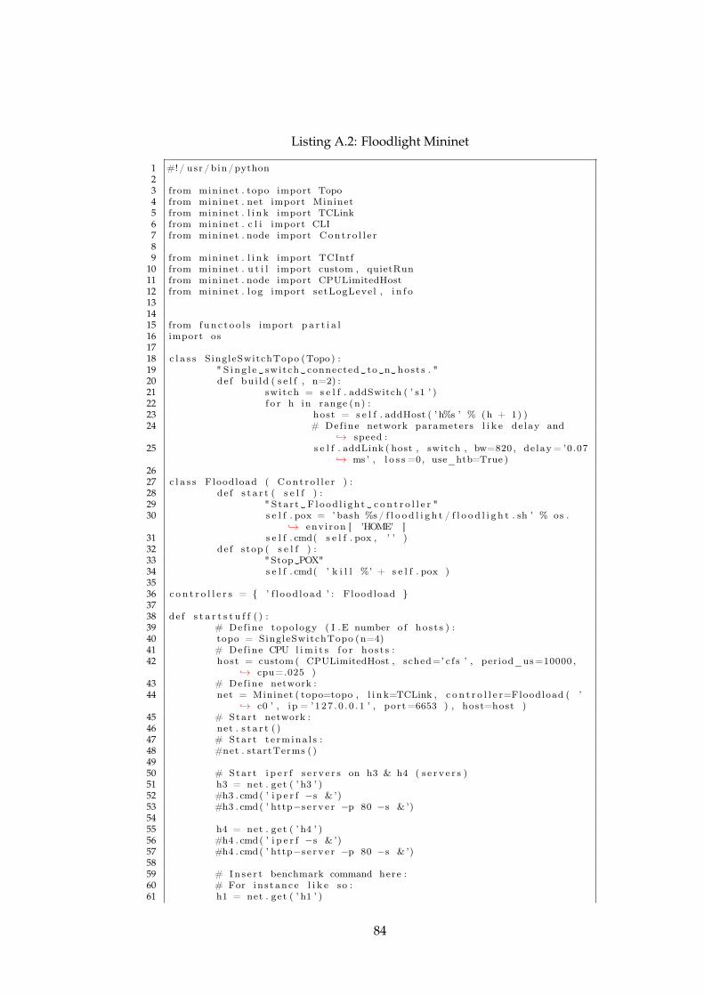
Listing A.2: Floodlight Mininet

1 #!/ usr /bin /python23 from mininet . topo import Topo4 from mininet . net import Mininet5 from mininet . l i n k import TCLink6 from mininet . c l i import CLI7 from mininet . node import Con t r o l l e r89 from mininet . l i n k import TCIntf

10 from mininet . u t i l import custom , quietRun11 from mininet . node import CPULimitedHost12 from mininet . l og import setLogLevel , i n f o131415 from fun c t o o l s import p a r t i a l16 import os1718 c l a s s SingleSwitchTopo (Topo) :19 " S ing l e ␣ switch ␣ connected ␣ to ␣n␣ hos t s . "20 de f bu i ld ( s e l f , n=2) :21 switch = s e l f . addSwitch ( ’ s1 ’ )22 f o r h in range (n) :23 host = s e l f . addHost ( ’ h%s ’ % (h + 1) )24 # Def ine network parameters l i k e de lay and

↪→ speed :25 s e l f . addLink ( host , switch , bw=820 , de lay = ’0.07

↪→ ms ’ , l o s s =0, use_htb=True )2627 c l a s s Floodload ( Con t r o l l e r ) :28 de f s t a r t ( s e l f ) :29 " Star t ␣ F l ood l i gh t ␣ c o n t r o l l e r "30 s e l f . pox = ’ bash %s/ f l o o d l i g h t / f l o o d l i g h t . sh ’ % os .

↪→ envi ron [ ’HOME’ ]31 s e l f . cmd( s e l f . pox , ’ ’ )32 de f stop ( s e l f ) :33 "Stop␣POX"34 s e l f . cmd( ’ k i l l %’ + s e l f . pox )3536 c o n t r o l l e r s = { ’ f l ood load ’ : Floodload }3738 de f s t a r t s t u f f ( ) :39 # Def ine topology ( I .E number o f hos t s ) :40 topo = SingleSwitchTopo (n=4)41 # Def ine CPU l im i t s f o r hos t s :42 host = custom ( CPULimitedHost , sched=’ c f s ’ , period_us=10000 ,

↪→ cpu=.025 )43 # Def ine network :44 net = Mininet ( topo=topo , l i n k=TCLink , c o n t r o l l e r=Floodload ( ’

↪→ c0 ’ , ip = ’127 . 0 . 0 . 1 ’ , port=6653 ) , host=host )45 # Star t network :46 net . s t a r t ( )47 # Star t t e rmina l s :48 #net . startTerms ( )4950 # Star t i p e r f s e r v e r s on h3 & h4 ( s e r v e r s )51 h3 = net . get ( ’ h3 ’ )52 #h3 . cmd( ’ i p e r f −s & ’)53 #h3 . cmd( ’ http−s e r v e r −p 80 −s & ’)5455 h4 = net . get ( ’ h4 ’ )56 #h4 . cmd( ’ i p e r f −s & ’)57 #h4 . cmd( ’ http−s e r v e r −p 80 −s & ’)5859 # In s e r t benchmark command here :60 # For in s t anc e l i k e so :61 h1 = net . get ( ’ h1 ’ )

84

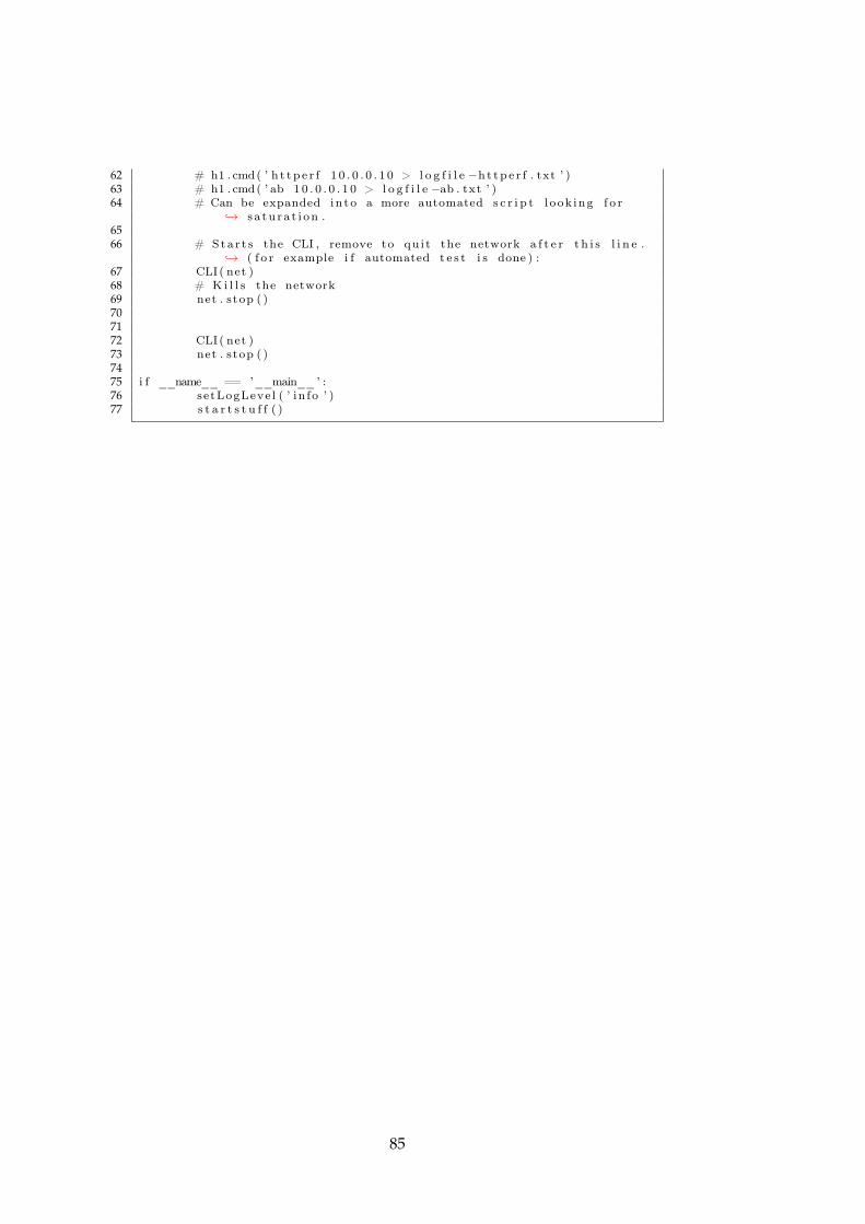
62 # h1 . cmd( ’ h t t p e r f 1 0 . 0 . 0 . 1 0 > l o g f i l e −h t tp e r f . txt ’ )63 # h1 . cmd( ’ ab 1 0 . 0 . 0 . 1 0 > l o g f i l e −ab . txt ’ )64 # Can be expanded in to a more automated s c r i p t l ook ing f o r

↪→ s a tu ra t i on .6566 # Sta r t s the CLI , remove to qu i t the network a f t e r t h i s l i n e .

↪→ ( f o r example i f automated t e s t i s done ) :67 CLI( net )68 # K i l l s the network69 net . stop ( )707172 CLI( net )73 net . stop ( )7475 i f __name__ == ’__main__’ :76 setLogLeve l ( ’ in fo ’ )77 s t a r t s t u f f ( )

85

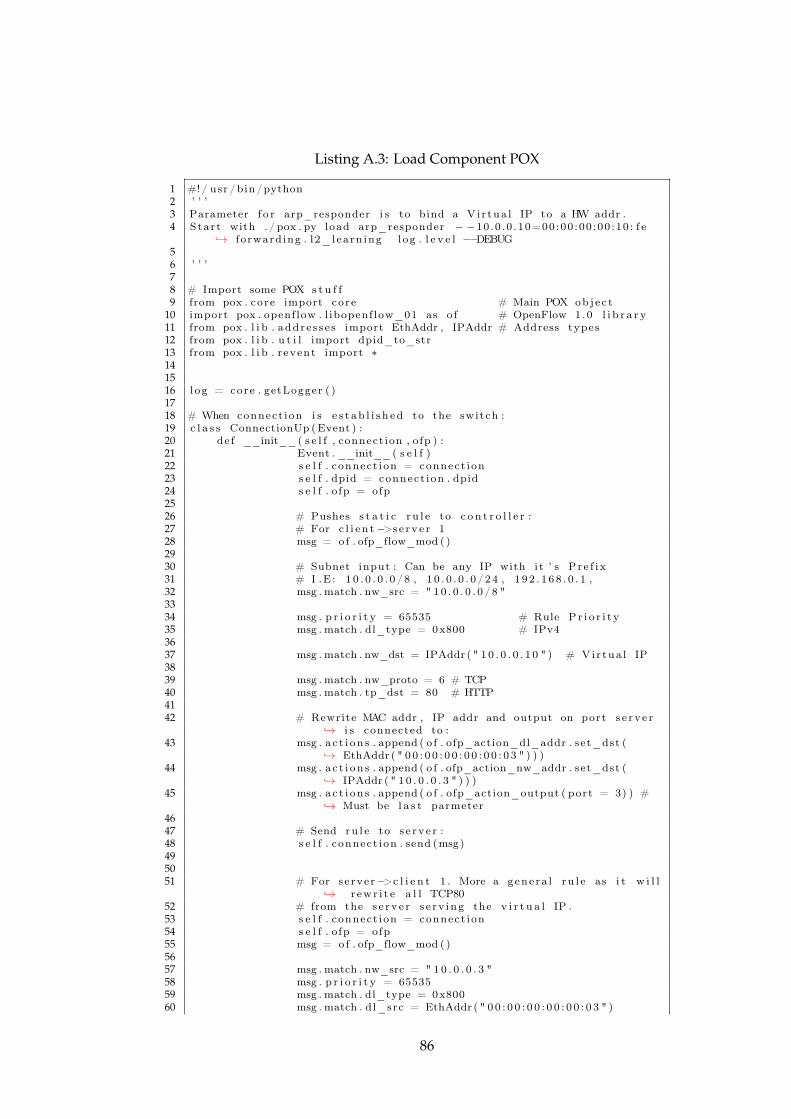
Listing A.3: Load Component POX

1 #!/ usr /bin /python2 ’ ’ ’3 Parameter f o r arp_responder i s to bind a Vi r tua l IP to a HW addr .4 Star t with . / pox . py load arp_responder − −10 .0 .0 .10=00 :00 :00 :00 :10 : f e

↪→ forward ing . l 2_learn ing log . l e v e l −−DEBUG56 ’ ’ ’78 # Import some POX s t u f f9 from pox . core import core # Main POX ob j e c t

10 import pox . openf low . l ibopenf low_01 as o f # OpenFlow 1 .0 l i b r a r y11 from pox . l i b . addre s s e s import EthAddr , IPAddr # Address types12 from pox . l i b . u t i l import dpid_to_str13 from pox . l i b . revent import ∗141516 l og = core . getLogger ( )1718 # When connect ion i s e s t a b l i s h e d to the switch :19 c l a s s ConnectionUp (Event ) :20 de f __init__( s e l f , connect ion , ofp ) :21 Event . __init__( s e l f )22 s e l f . connect ion = connect ion23 s e l f . dpid = connect ion . dpid24 s e l f . o fp = ofp2526 # Pushes s t a t i c r u l e to c o n t r o l l e r :27 # For c l i e n t−>se rv e r 128 msg = of . ofp_flow_mod ( )2930 # Subnet input : Can be any IP with i t ’ s P r e f i x31 # I .E: 1 0 . 0 . 0 . 0 / 8 , 1 0 . 0 . 0 . 0 / 2 4 , 1 9 2 . 1 6 8 . 0 . 1 ,32 msg . match . nw_src = " 10 . 0 . 0 . 0 / 8 "3334 msg . p r i o r i t y = 65535 # Rule P r i o r i t y35 msg . match . dl_type = 0x800 # IPv43637 msg . match . nw_dst = IPAddr ( " 1 0 . 0 . 0 . 1 0 " ) # Vi r tua l IP3839 msg . match . nw_proto = 6 # TCP40 msg . match . tp_dst = 80 # HTTP4142 # Rewrite MAC addr , IP addr and output on port s e r v e r

↪→ i s connected to :43 msg . a c t i on s . append ( o f . ofp_action_dl_addr . set_dst (

↪→ EthAddr ( " 0 0 : 0 0 : 0 0 : 0 0 : 0 0 : 0 3 " ) ) )44 msg . a c t i on s . append ( o f . ofp_action_nw_addr . set_dst (

↪→ IPAddr ( " 1 0 . 0 . 0 . 3 " ) ) )45 msg . a c t i on s . append ( o f . ofp_action_output ( port = 3) ) #

↪→ Must be l a s t parmeter4647 # Send ru l e to s e r v e r :48 s e l f . connect ion . send (msg)495051 # For se rver−>c l i e n t 1 . More a gene ra l r u l e as i t w i l l

↪→ r ewr i t e a l l TCP8052 # from the s e r v e r s e rv i ng the v i r t u a l IP .53 s e l f . connect ion = connect ion54 s e l f . o fp = ofp55 msg = of . ofp_flow_mod ( )5657 msg . match . nw_src = " 1 0 . 0 . 0 . 3 "58 msg . p r i o r i t y = 6553559 msg . match . dl_type = 0x80060 msg . match . dl_src = EthAddr ( " 0 0 : 0 0 : 0 0 : 0 0 : 0 0 : 0 3 " )

86

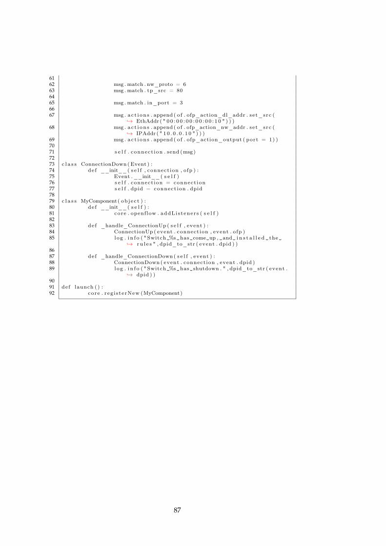
6162 msg . match . nw_proto = 663 msg . match . tp_src = 806465 msg . match . in_port = 36667 msg . a c t i on s . append ( o f . ofp_action_dl_addr . se t_src (

↪→ EthAddr ( " 0 0 : 0 0 : 0 0 : 0 0 : 0 0 : 1 0 " ) ) )68 msg . a c t i on s . append ( o f . ofp_action_nw_addr . se t_src (

↪→ IPAddr ( " 1 0 . 0 . 0 . 1 0 " ) ) )69 msg . a c t i on s . append ( o f . ofp_action_output ( port = 1) )7071 s e l f . connect ion . send (msg)7273 c l a s s ConnectionDown (Event ) :74 de f __init__( s e l f , connect ion , ofp ) :75 Event . __init__( s e l f )76 s e l f . connect ion = connect ion77 s e l f . dpid = connect ion . dpid7879 c l a s s MyComponent( ob j e c t ) :80 de f __init__( s e l f ) :81 core . openf low . addL i s t ene r s ( s e l f )8283 de f _handle_ConnectionUp ( s e l f , event ) :84 ConnectionUp ( event . connect ion , event . ofp )85 l og . i n f o ( "Switch␣%s␣has␣come␣up , ␣and␣ i n s t a l l e d ␣ the ␣

↪→ r u l e s " , dpid_to_str ( event . dpid ) )8687 de f _handle_ConnectionDown ( s e l f , event ) :88 ConnectionDown ( event . connect ion , event . dpid )89 l og . i n f o ( "Switch␣%s␣has␣shutdown . " , dpid_to_str ( event .

↪→ dpid ) )9091 de f launch ( ) :92 core . reg i s te rNew (MyComponent)

87

Appendix B

Raw data

For some tests where the data was collected out of normal 3 test averagescenario, their result is presented here:

89

Table B.1: Proactive POX httperf test of 1 server-rawHttperf: (60*R=Num-conns) Request rate asked: (req/s) Compleded rate Duration

1 2520 42 41,1 61,32 2520 42 40,9 61,63 2520 42 41 61,44 2520 42 42,2 61,25 2520 42 40,8 61,76 2520 42 41,4 60,97 2520 42 41,1 61,38 2520 42 41,8 60,29 2520 42 41,1 61,3Standard deviation 0,355555556 0,29629629690% CI interval (t.test) 40,98262-41,5507 60,93661-61,48561Mean 41,26667 61,21111

90

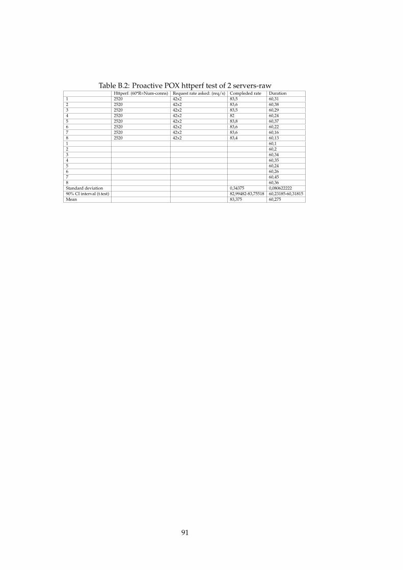
Table B.2: Proactive POX httperf test of 2 servers-rawHttperf: (60*R=Num-conns) Request rate asked: (req/s) Compleded rate Duration

1 2520 42x2 83,5 60,312 2520 42x2 83,6 60,383 2520 42x2 83,5 60,294 2520 42x2 82 60,245 2520 42x2 83,8 60,376 2520 42x2 83,6 60,227 2520 42x2 83,6 60,168 2520 42x2 83,4 60,131 60,12 60,23 60,344 60,355 60,246 60,267 60,458 60,36Standard deviation 0,34375 0,08062222290% CI interval (t.test) 82,99482-83,75518 60,23185-60,31815Mean 83,375 60,275

91

A Software Deﬁned Networking evaluation approach to ...

Documents

Transcript of A Software Deﬁned Networking evaluation approach to ...