A Smooth Contact-State Transition in a Dynamic Model ofRolling-Element Bearings

Matej Razpotnika, Gregor Cepona,∗, Miha Boltezara

aUniversity of Ljubljana, Faculty of Mechanical Engineering

Abstract

We present a new formulation to calculate the response of a system containing rolling-element bearingsoperating under a radial clearance and a dominant radial load. The nonlinear bearing force- and stiffness-displacement characteristics in combination with the bearing clearance necessitate an advanced numericalanalysis. The response of a shaft-bearing-housing assembly can be unstable in the transient regions, e.g.,at the start of a system run-up or when passing the critical speed of a system. This can lead to longcomputational times or even to non-converged solutions. In this paper, a new analytical bearing-stiffnessmodel is presented that is capable of overcoming these problems by smoothing the nonlinear bearing force-and stiffness-displacement characteristics in the discontinuous regions. The smoothing is implemented on thedeformation scale. The proposed model is modular, allowing us to define a specific value of the smoothing toeach rolling element that comes into contact. A simple case study that involves two bearings of different types(ball and cylindrical roller) is presented. They support an unbalanced rotor, subjected to a constant angularacceleration. We show that a small smoothing value can significantly enhance the numerical calculation ofthe chosen system in terms of speed and stability.

Keywords: Dynamic bearing model, Smooth contact-state transition, Rolling-element bearing stiffnessmatrix, Unbalanced rotor

Nomenclature

A0 Unloaded distance between the inner and outer raceway grooves’ curvature centres [mm]Aj Loaded distance between the inner and outer raceway grooves’ curvature centres [mm]D Bearing outer diameter [mm]d Bearing inner diameter [mm]Fi Mean bearing force in the i = x, y, z directions [N]fb Mean bearing load vector, composed by the mean bearing forces Fi and the mean bearing moments

Mi (i = x, y, z).Kn Rolling-element load-deflection stiffness constant [N/mmn]Kb Comprehensive bearing-stiffness matrix of dimension sixkij Bearing stiffness coefficient, i, j = x, y, z, βx, βy, βz [N/mm]k0j Partial derivative of resultant elastic deformation δB′j with respect to the radial displacement δx′ at

δBx′0j in a rotating coordinate system

kj Partial derivative of resultant elastic deformation δB′j with respect to the radial displacement δx′ atλj in a rotating coordinate system

leff Effective roller length [mm]

∗Corresponding authorEmail address: gregor.cepon@fs.uni-lj.si (Gregor Cepon)

Preprint submitted to Journal of Sound and Vibration June 6, 2018

Mi Mean bearing moment about i = x, y, z directions [N mm]m Bearing smoothing vector, composed by the user-defined values of deformation µ0j , below which

smoothing is applied (j = 1, 2, . . . z)n Rolling-element load-deflection exponentqb Mean bearing displacement vector, composed by the mean bearing translational displacements δi

and the mean bearing rotational displacements βi (i = x, y, z)R Rotational transformation matrix from fixed to rotating Cartesian coordinate systemrb Radius of rolling element in ball bearings [mm]rj Pitch radius (roller) or radii of inner raceway groove’s curvature centres (ball) [mm]rc Bearing radial clearance [mm]z Total number of rolling elements in a bearingα0 Unloaded bearing contact angle [rad]αj Loaded jth rolling element contact angle [rad]βi Mean bearing rotational displacement about the i = x, y, z axis [rad]δBj

Resultant elastic deformation of the jth ball element [mm]δBx′0j Displacement of the jth ball in a radial direction (x′) needed to overcome the clearance [mm]

δRjResultant elastic deformation of the jth roller element [mm]

δRx′0j Displacement of the jth roller in a radial direction (x′) needed to overcome clearance [mm]

δT ′j Smoothed resultant elastic deformation of the jth rolling element in a region of contact-state tran-sition [mm]

δi Mean bearing translational displacement in the i = x, y, z direction [mm]δrj Effective jth rolling element displacement in the radial direction [mm]δzj Effective jth rolling element displacement in the axial direction [mm]λj Radial displacement at which a deformation of the jth rolling element is equal to µj [mm]µ0j User-defined value of deformation of the jth rolling element below which smoothing is applied [mm]µj Exact value of deformation of the jth rolling element below which a smoothing is applied [mm]ϕ Angle between rotational and fixed coordinate system [rad]ψj Angular distance of the jth rolling element from the x-axis [rad](...)′ Arbitrary previously defined symbol in rotating coordinate system (x′, y′, z′)

1. Introduction

The dynamic characterization of rolling bearings has been investigated for many decades; however,due to its complexity it remains an important matter in ongoing research. Despite a great increase incomputer power in recent years and consequently computer-aided engineering (CAE), the modelling ofbearing dynamics continues at the analytical level. These analytically derived dynamic bearing models areafterwards inserted into a numerical model of the system in the sense of a shaft-bearing-housing assembly.Due to the nonlinear nature of the contact formulation in rolling bearings, the prediction of the system’sresponse remains a tedious task.

A first general theory for elastically constrained ball and roller bearings was developed by Jones [1]and later on further derived by Harris [2]. This theory was in fact very general and it was not able toproperly determine the cross-coupling stiffness between the radial, axial and the tilting deflections. Sim-plified bearing models were instead introduced by other researchers, where the bearings were modelled asideal boundary conditions for the shaft, as presented by Rao [3]. Meanwhile, the idea of interpreting thebearings with a simple one- or two-degrees-of-freedom (DOFs) model with linear springs was introducedby While [4] and Gargiulo [5]. Later, more precise bearing models were derived. A major improvementin predicting the vibration transmission through rolling-element bearings was made by Lim and Singh [6],who derived a model that provides a comprehensive bearing-stiffness matrix. The model is capable of prop-erly describing the nonlinear relation between the load and the deflection, taking into account all 6 DOFsand their interplay. The model of Lim and Singh was the basis for many subsequent investigations. Thesame authors described the effect of a distributed contact load on a roller bearing’s stiffness matrix [7].Later, Royston and Basdogan [8] introduced a model for predicting the vibration transmission through

2

self-aligning (spherical) rolling-element bearings. Liew and Lim [9] extended the model of Lim and Singhto analyse the time-varying rolling element bearing characteristics that occur due to the pass of the rollingelement. A bearing-stiffness matrix formulation for double raw angular contact ball bearings was derivedby Gunduz and Singh [10]. Lee and Choi [11] presented an analysis approach where they investigated thespeed-dependent ball-bearing stiffness in a flexible rotor with a nonlinear bearing characteristic based onJones’ model. Sheng et al. [12] studied and derived the bearing speed-varying stiffness model. With thedevelopment of the finite-element-method (FEM) models, new techniques for calculating the proper bearingdynamics have appeared. Guo and Parker [13] proposed a stiffness matrix calculation for a rolling-elementbearing using a finite-element/contact-mechanics model. The authors precisely modelled each integral partof the bearing and implemented a special contact model derived by Vijayakar [14] between the rolling ele-ments and both raceways. Recently, Zhang et al. [15] presented a general model for preload calculation andstiffness analysis for combined angular contact ball bearings.

Many authors have studied the bearing dynamics by analysing a rotor-bearing-housing assembly. Limand Singh investigated a geared-rotor system [16, 17] and performed a statistical energy analysis [18]. Baiet al. [19] went step further and analysed the acoustic response. They evaluated the radiation noise of thebearing applied to the ceramic motorized spindle based on the sub-source decomposition method. Cermeljand Boltezar [20] presented an indirect approach to investigate the dynamics of a structure with ball bearings.Lately, Razpotnik et al. [21] investigated the vibration transmission in a statically indeterminate system thatis supported by bearings. The dynamic behaviour of a system containing bearings where the time responsewas calculated was presented by Xu and Li [22, 23] for a planar multibody system with multiple deep grooveball-bearing joints. Fonseca et al. [24] studied the influence of unbalance levels on nonlinear dynamics ofa rotor-backup rolling bearing system. Wang et.al. [25] conducted dynamic modelling of moment wheelassemblies with nonlinear rolling bearing supports. They performed dynamic tests to verify the nonlineardynamic model. The effect of bearing preload on the modal characteristics of a shaft-bearing assemblywas investigated by Gunduz et al. [26]. Similarly, the effect of the axial preload of the ball bearings onthe nonlinear dynamic characteristics of a rotor-bearing system was investigated by Bai et al. [27]. It wasshown that the bifurcation margins of an unbalanced rotor-bearing system enhance markedly when the axialpreload increases and relates to the system’s resonance speed.

Predicting the response of a system with rolling bearings often encounters numerical difficulties whena time integration is performed. The problem originates in a sudden contact-state transition, which isgoverned by the bearing clearance and the nonlinear force- and stiffness-displacement characteristics. Severalattempts have been made to increase the stability of the calculation. Fleming and Poplawski [28] showedthat a moderate amount of damping eliminated the bistable region in their response, but this damping is notinherent in the ball bearings and introduces additional artificial forces. Another approach was presented byXia et al. [29] for the rotor-bearing system with journal bearings. They presented two calculation methods(the Ritz model and a one-dimensional FEM) to overcome the numerical shortcomings of the extremelytime-consuming Reynolds equations.

In this paper a new formulation for the contact-state transition is presented for rolling-element bearingswith a radial clearance to ensure a stable numerical calculation. The original non-smooth contact-dynamicsformulation implies numerical issues in a time-integration process. In order to avoid these problems theproposed formulation introduces smooth bearing deformation-displacement characteristics in the region ofthe impact contacts. The idea is somehow similar to the modelling of a non-smooth friction force usingan approximate single-valued friction law [30]. The bearing model from Lim and Singh [6] represents thebasis for our study. Since the formulation proposes the smoothing of deformations, the whole existingbearing model has to be reformulated and new equations have to be derived to obtain a comprehensivebearing-stiffness matrix. The modularity of the proposed bearing model allows the implementation of anarbitrary smoothing value for each individual rolling element. The applicability of the newly developedbearing model is demonstrated on a simple unbalanced rotor that is supported by two bearings. It is shownthat already a small value of the smoothing parameter significantly improves the numerical simulation interms of speed and stability. The aim of the presented work is not to change the bearing design, but tofacilitate the calculation process. Many engineering applications related to the rotating machinery mightfind the presented contribution valuable.

3

2. Assumptions

Besides the assumptions given in [6] the following also have to be taken into account:

1. The radial load is dominant.

2. It is applicable to bearings that operate under a radial clearance. Therefore, ball and cylindrical rollerbearings are of primary interest.

3. The new, rotating coordinate system is used, which follows the direction of the radial load. Radialx-axis points directly to one rolling element (as assumed already in [6]). Consequently, any fluctuationdue to a rolling-element pass is neglected.

3. The existing analytical bearing model

3.1. Presentation of the 6-DOFs bearing model

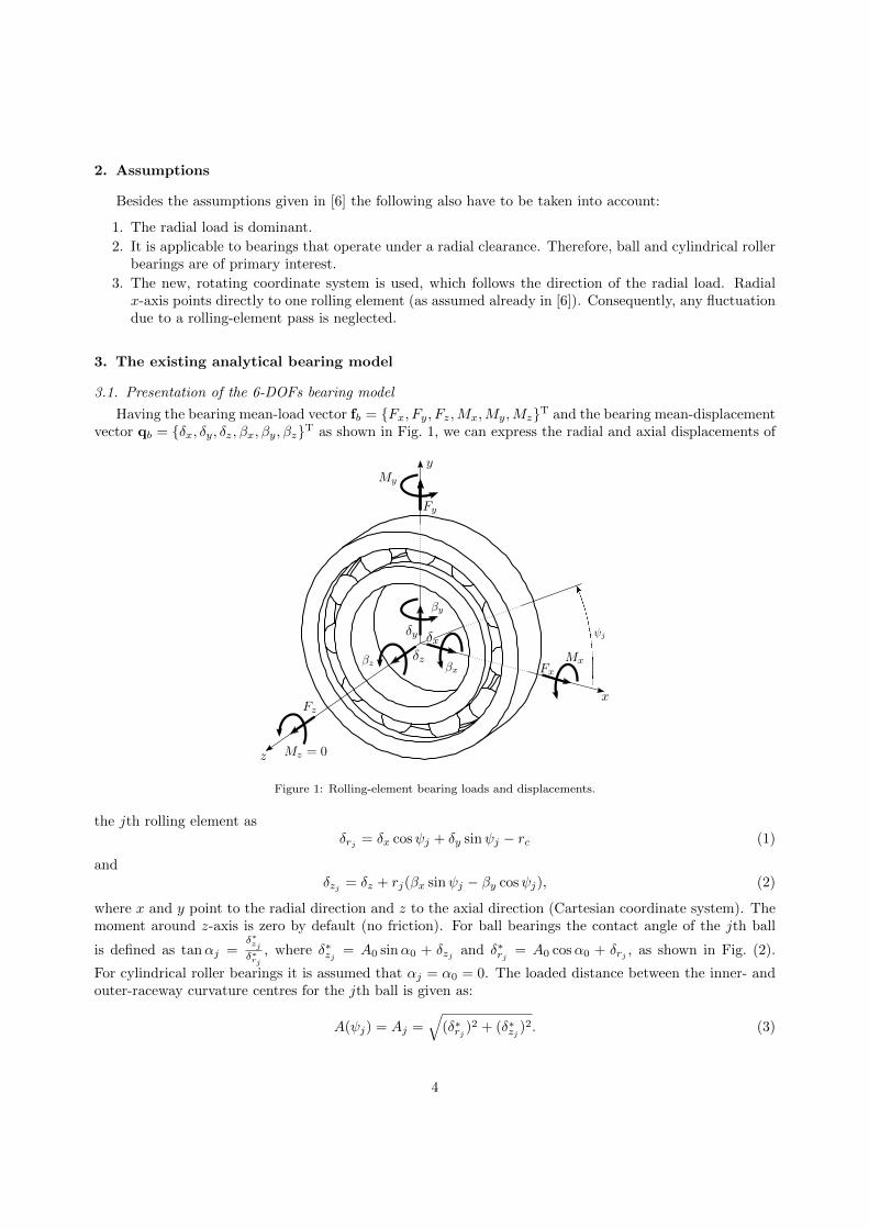
Having the bearing mean-load vector fb = {Fx, Fy, Fz,Mx,My,Mz}T and the bearing mean-displacementvector qb = {δx, δy, δz, βx, βy, βz}T as shown in Fig. 1, we can express the radial and axial displacements of

Figure 1: Rolling-element bearing loads and displacements.

the jth rolling element asδrj = δx cosψj + δy sinψj − rc (1)

andδzj = δz + rj(βx sinψj − βy cosψj), (2)

where x and y point to the radial direction and z to the axial direction (Cartesian coordinate system). Themoment around z-axis is zero by default (no friction). For ball bearings the contact angle of the jth ball

is defined as tanαj =δ∗zjδ∗rj

, where δ∗zj = A0 sinα0 + δzj and δ∗rj = A0 cosα0 + δrj , as shown in Fig. (2).

For cylindrical roller bearings it is assumed that αj = α0 = 0. The loaded distance between the inner- andouter-raceway curvature centres for the jth ball is given as:

A(ψj) = Aj =√

(δ∗rj )2 + (δ∗zj )2. (3)

4

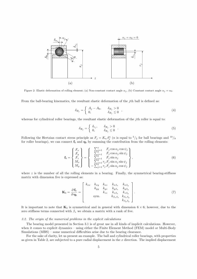
Figure 2: Elastic deformation of rolling element; (a) Non-constant contact angle αj , (b) Constant contact angle αj = α0.

From the ball-bearing kinematics, the resultant elastic deformation of the jth ball is defined as:

δBj=

{Aj −A0, δBj

> 00, δBj

≤ 0, (4)

whereas for cylindrical roller bearings, the resultant elastic deformation of the jth roller is equal to:

δRj =

{δrj , δRj

> 00, δRj

≤ 0. (5)

Following the Hertzian contact stress principle as Fj = Kn δnj (n is equal to 3/2 for ball bearings and 10/9

for roller bearings), we can connect fb and qb by summing the contribution from the rolling elements:

fb =

FxFyFzMx

My

=

∑zj=1 Fj cosαj cosψj∑zj=1 Fj cosαj sinψj∑zj=1 Fj sinαj∑zj=1 rj Fj sinαj sinψj

−∑zj=1 rj Fj sinαj cosψj

, (6)

where z is the number of all the rolling elements in a bearing. Finally, the symmetrical bearing-stiffnessmatrix with dimension five is expressed as:

Kb =∂ fb∂ qb

=

kxx kxy kxz kxβx

kxβy

kyy kyz kyβxkyβy

kzz kzβxkzβy

sym. kβxβx kβxβy

kβyβy

. (7)

It is important to note that Kb is symmetrical and in general with dimension 6 × 6; however, due to thezero stiffness terms connected with βz we obtain a matrix with a rank of five.

3.2. The origin of the numerical problems in the explicit calculations

The bearing model presented in Section 3.1 is of great use in all kinds of implicit calculations. However,when it comes to explicit dynamics – using either the Finite Element Method (FEM) model or Multi-BodySimulations (MBS) – some numerical difficulties arise due to the bearing clearance.

For the sake of clarity, let us present an example. The ball and cylindrical roller bearings, with propertiesas given in Table 2, are subjected to a pure radial displacement in the x direction. The implied displacement

5

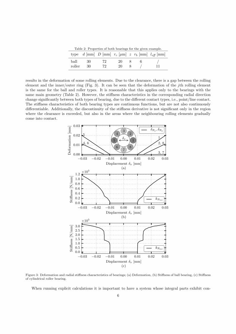
Table 2: Properties of both bearings for the given example.

type d [mm] D [mm] rc [µm] z rb [mm] leff [mm]

ball 30 72 20 8 6 /roller 30 72 20 8 / 11

results in the deformation of some rolling elements. Due to the clearance, there is a gap between the rollingelement and the inner/outer ring (Fig. 3). It can be seen that the deformation of the jth rolling elementis the same for the ball and roller types. It is reasonable that this applies only to the bearings with thesame main geometry (Table 2). However, the stiffness characteristics in the corresponding radial directionchange significantly between both types of bearing, due to the different contact types, i.e., point/line contact.The stiffness characteristics of both bearing types are continuous functions, but are not also continuouslydifferentiable. Additionally, the discontinuity of the stiffness derivative is not significant only in the regionwhere the clearance is exceeded, but also in the areas where the neighbouring rolling elements graduallycome into contact.

−0.03 −0.02 −0.01 0.00 0.01 0.02 0.03

Displacement δx [mm](a)

0.00

0.01

0.02

0.03

Def

orm

ati

on

[mm

]

1

23

4

5

67

8

1

2, 8

3, 7

4, 6

5δx

δBj , δRj

−0.03 −0.02 −0.01 0.00 0.01 0.02 0.03

Displacement δx [mm](b)

0.0

0.2

0.4

0.6

0.8

1.0

1.2

Sti

ffnes

s[N/m

m]

×105

kBxx

−0.03 −0.02 −0.01 0.00 0.01 0.02 0.03

Displacement δx [mm](c)

0.00.51.01.52.02.53.0

Sti

ffnes

s[N/m

m]

×105

kRxx

Figure 3: Deformation and radial stiffness characteristics of bearings; (a) Deformation, (b) Stiffness of ball bearing, (c) Stiffnessof cylindrical roller bearing.

When running explicit calculations it is important to have a system whose integral parts exhibit con-

6

tinuously differentiable stiffness-displacement characteristics. Otherwise, a time step during the integrationprocess decreases significantly, which results in a longer computational time or even leads to non-convergedsolutions. A similar problem is well known in contact mechanics when modelling a friction phenomenon.

4. Smoothing the contact-state transition

A contact change from open to closed represents a transient phenomenon. When the transition is very fastin terms of time, we can talk about impacts. They change the dynamic properties of a system significantlyin a very short time. In the case of bearings, this happens when the rolling elements eliminate the clearanceand suddenly hit the raceways. This sudden change of the bearing load vector and the corresponding bearingstiffness represents the root cause of many problems in a time-integration procedure.

An efficient way to improve the calculation of a system with a sudden contact-state transition is to derivethe smoothed force and the corresponding stiffness characteristics in the area of the transition. A suddenhit, which appears every time each single rolling element eliminates the clearance and hits between bothraceways can be effectively smoothed. The transition is especially problematic for the first rolling elementcoming into a contact (Fig. 3). The smooth contact transition introduces “simplification”, which helpsthe integration process to pass that region flawlessly. Smoothing a function implies an approximate finalsolution in the region where the smoothing is applied. Obviously, there is a trade-off between the exactsolution with numerical difficulties and the approximate one with numerical ease.

4.1. Theoretical background

A sudden transition of the force- and stiffness-displacement characteristics originates in piecewise-definedball- and roller-bearing kinematics as given in Eq. (4) and (5). Thus, it is reasonable to smooth thefunction regulation in the region between both pieces. Furthermore, this change is to be conducted on thedeformation level so that the derived expressions for the force- and stiffness-displacement characteristics areto be smoothed as well. From Eq. (4) and (5) it follows that

Aj −A0 = 0 and δrj = 0 (8)

represent the points between both function intervals of the jth rolling element for a ball and cylindricalroller bearing, respectively. Since radial load is dominant and most sensitive to the impacts, we have tofind the roots of Eq. (8) in radial (x′) direction. The roots represent the radial displacement of each jthrolling element (as a function of all other DOFs), needed to overcome a clearance. First, we define a newrotating Cartesian coordinate system as shown in Fig. 4. The axes z′ and z are aligned, whereas the axes x′

and y′ rotate around z′. Such a coordinate system enables the definition of a radial displacement entirelyin the x′z′ plane, having a displacement in the y′ direction always equal to zero. The new mean-load andmean-displacement vectors are defined as:

fb′ = {Fx′ , Fy′ = 0, Fz′ , Mx′ , My′Mz′ = 0}T,qb′ = {δx′ , δy′ = 0, δz′ , βx′ , βy′ βz′}T.

(9)

The transformation from the fixed to the rotating coordinate system is equal to

qb′ = Rqb, (10)

where R is a rotational transformation matrix. Hereinafter, all the parameters and properties that refer tothe rotating coordinate system are denoted as (...)′.

7

Figure 4: Fixed and rotating coordinate systems.

4.1.1. Ball bearings

By transforming Eq. (8) to the rotating coordinate system we can express the roots of Eq. (8) in x′

direction as a function of all other displacements and rotations:

Aj′ −A0 = 0(A0 cosα0 + δx′ cosψ′j − rc

)2=(A2

0 − (δ∗z′j ))2

δx′B0j=

1

cosψ′j

(rc −A0 cosα0 +

√A2

0 − (δ∗z′j)2)

(11)

Having an arbitrary qb′ , Eq. (11) gives the exact radial displacement δx′B0jat which every jth ball is coming

into contact. Going back to Eq. (4) with all the radial roots δx′B0jknown, we have to make the transition

smooth. In order to achieve that, the value of the deformation δB′j below which the smoothing is to beapplied has to be defined. This value is initially given by the user and we denote it as µ0j . If δB′j is a

linear function (valid only when all the other than radial displacement are equal to zero), we calculate thecorresponding radial displacement as:

λj = δx′B0j+µ0j

k0j, (12)

where k0j is the slope of δB′j at δx′B0j. However, in general δB′j is not linear (Eq. (3)) and the slope in the

radial direction is a function of qb′ , which can be expressed as:

kj = kj(qb′) =∂ δB′j∂ x′

=δ∗r′jA′j

cosψ′j . (13)

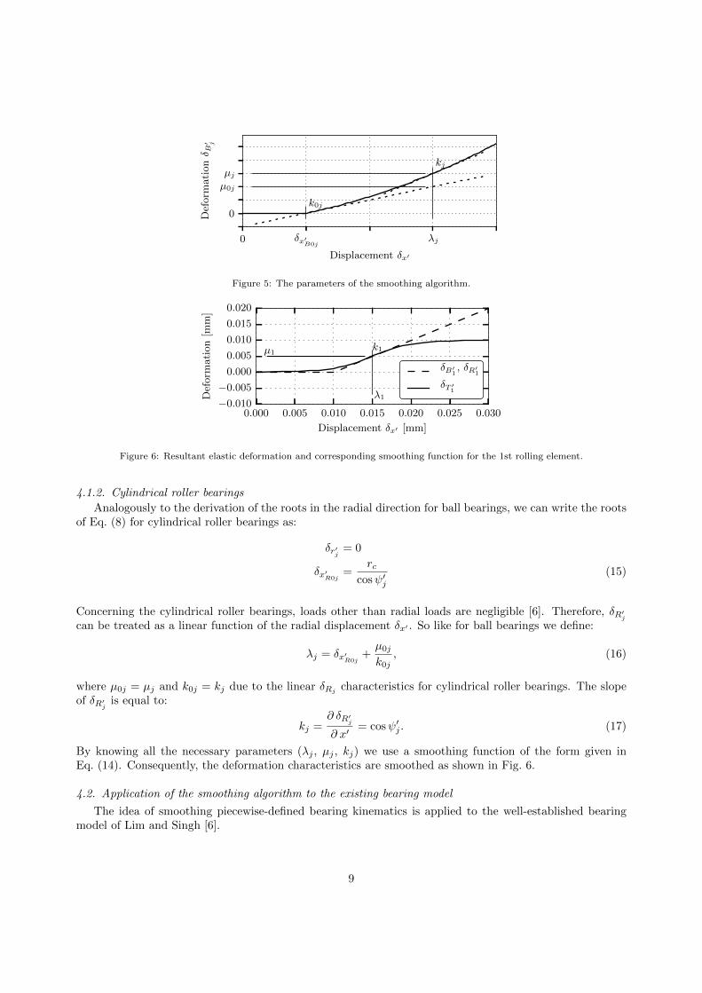
Thus, an exact deformation µj , which is equal to δB′j (λj) differs slightly from µ0j , as demonstrated inFig. 5. Based on the initial µ0j we can calculate the parameters λj , µj and kj , which are crucial to define asmoothing function. For the latter we use a hyperbolic tangent function of the form:

δT ′j = µj

(tanh

(kjµj

(δx′ − λj))

+ 1

). (14)

Fig. 6 shows δB′1 and δT ′1 as a function of the radial displacement δx′ (other displacements and rotationsare here equal to zero). It is clear that a combination of the functions δB′j and δT ′j results in a continuouslydifferentiable function, since their values and derivatives at λj are exactly the same.

8

0 δx′B0jλj

Displacement δx′

0

µ0j

µj

Def

orm

ati

onδ B′ j

k0j

kj

Figure 5: The parameters of the smoothing algorithm.

0.000 0.005 0.010 0.015 0.020 0.025 0.030

Displacement δx′ [mm]

−0.010

−0.005

0.000

0.005

0.010

0.015

0.020

Def

orm

ati

on

[mm

]

µ1

λ1

k1

δB′1 , δR′1δT ′1

Figure 6: Resultant elastic deformation and corresponding smoothing function for the 1st rolling element.

4.1.2. Cylindrical roller bearings

Analogously to the derivation of the roots in the radial direction for ball bearings, we can write the rootsof Eq. (8) for cylindrical roller bearings as:

δr′j = 0

δx′R0j=

rccosψ′j

(15)

Concerning the cylindrical roller bearings, loads other than radial loads are negligible [6]. Therefore, δR′jcan be treated as a linear function of the radial displacement δx′ . So like for ball bearings we define:

λj = δx′R0j+µ0j

k0j, (16)

where µ0j = µj and k0j = kj due to the linear δRjcharacteristics for cylindrical roller bearings. The slope

of δR′j is equal to:

kj =∂ δR′j∂ x′

= cosψ′j . (17)

By knowing all the necessary parameters (λj , µj , kj) we use a smoothing function of the form given inEq. (14). Consequently, the deformation characteristics are smoothed as shown in Fig. 6.

4.2. Application of the smoothing algorithm to the existing bearing model

The idea of smoothing piecewise-defined bearing kinematics is applied to the well-established bearingmodel of Lim and Singh [6].

9

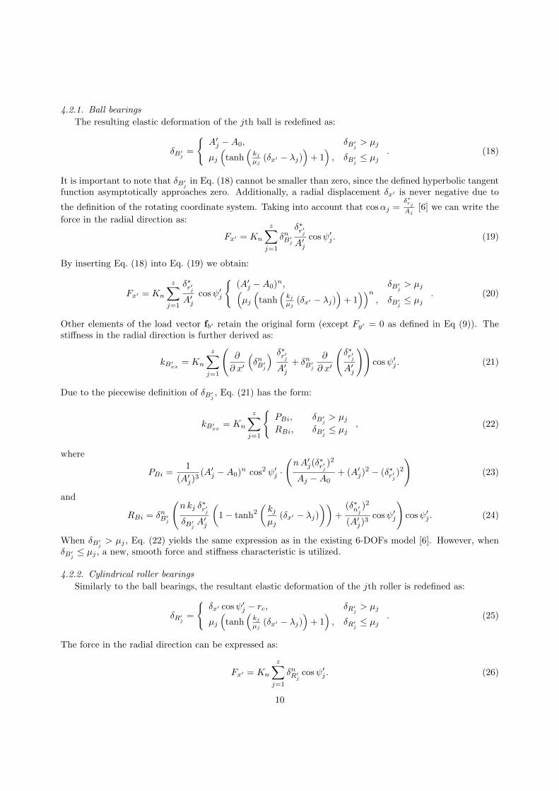
4.2.1. Ball bearings

The resulting elastic deformation of the jth ball is redefined as:

δB′j =

{A′j −A0, δB′j > µj

µj

(tanh

(kjµj

(δx′ − λj))

+ 1), δB′j ≤ µj

. (18)

It is important to note that δB′j in Eq. (18) cannot be smaller than zero, since the defined hyperbolic tangentfunction asymptotically approaches zero. Additionally, a radial displacement δx′ is never negative due to

the definition of the rotating coordinate system. Taking into account that cosαj =δ∗rjAj

[6] we can write the

force in the radial direction as:

Fx′ = Kn

z∑j=1

δnB′j

δ∗r′jA′j

cosψ′j . (19)

By inserting Eq. (18) into Eq. (19) we obtain:

Fx′ = Kn

z∑j=1

δ∗r′jA′j

cosψ′j

{(A′j −A0)n, δB′j > µj(µj

(tanh

(kjµj

(δx′ − λj))

+ 1))n

, δB′j ≤ µj. (20)

Other elements of the load vector fb′ retain the original form (except Fy′ = 0 as defined in Eq (9)). Thestiffness in the radial direction is further derived as:

kB′xx= Kn

z∑j=1

(∂

∂ x′

(δnB′j

) δ∗r′jA′j

+ δnB′j∂

∂ x′

(δ∗r′jA′j

))cosψ′j . (21)

Due to the piecewise definition of δB′j , Eq. (21) has the form:

kB′xx= Kn

z∑j=1

{PBi, δB′j > µjRBi, δB′j ≤ µj

, (22)

where

PBi =1

(A′j)3

(A′j −A0)n cos2 ψ′j ·(nA′j(δ

∗r′j

)2

Aj −A0+ (A′j)

2 − (δ∗r′j )2

)(23)

and

RBi = δnB′j

(nkj δ

∗r′j

δB′j A′j

(1− tanh2

(kjµj

(δx′ − λj)))

+(δ∗n′j

)2

(A′j)3

cosψ′j

)cosψ′j . (24)

When δB′j > µj , Eq. (22) yields the same expression as in the existing 6-DOFs model [6]. However, whenδB′j ≤ µj , a new, smooth force and stiffness characteristic is utilized.

4.2.2. Cylindrical roller bearings

Similarly to the ball bearings, the resultant elastic deformation of the jth roller is redefined as:

δR′j =

{δx′ cosψ′j − rc, δR′j > µj

µj

(tanh

(kjµj

(δx′ − λj))

+ 1), δR′j ≤ µj

. (25)

The force in the radial direction can be expressed as:

Fx′ = Kn

z∑j=1

δnR′j cosψ′j . (26)

10

After considering Eq. (25) we obtain:

Fx′ = Kn

z∑j=1

cosψ′j ·{ (

δx′ cosψ′j − rc)n, δR′j > µj(

µj

(tanh

(kjµj

(δx′ − λj))

+ 1))n

, δR′j ≤ µj. (27)

So like in the ball-bearing formulation, the other elements of the load vector fb′ retain their original form.The radial stiffness term transforms to:

kR′xx= Kn

z∑j=1

(∂

∂ x′

(δnR′j

)cosψ′j

). (28)

By inserting Eq. (25) into Eq. (28) we obtain the following expression:

kR′xx= Kn

z∑j=1

{PRi, δR′j > µjRRi, δR′j ≤ µj

, (29)

wherePRi = n δn−1R′j

cos2 ψ′j (30)

and

RRi = kj δn−1R′j

(1− tanh2

(kjµj

(δx′ − λj)))

cosψ′j (31)

Again, when δR′j > µj , Eq. (29) yields the same expression as in the existing 6-DOFs model for the cylindrical

roller bearings [6]. Additionally, when δR′j ≤ µj , a smooth stiffness characteristic is obtained.The proposed model introduces a smooth transition between the open- and the closed-contact states in

the radial direction. Initially, it is necessary to specify the level of deformation µ0j (for every jth rollingelement), below which the smoothing is applied. All the µ0j are joined together in a bearing-smoothingvector as:

m = {µ01, µ02 . . . µ0z}T . (32)

It is important to note that the first element in m represents the first rolling element coming into contact. Ifthe smoothing vector m contains zeros only, no smoothing is applied and the theory yields the formulationof the existing 6-DOFs model.

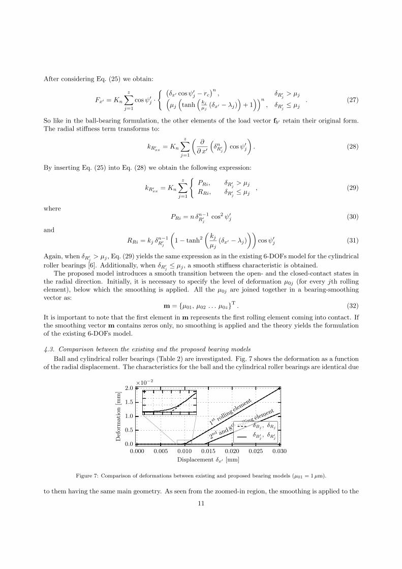
4.3. Comparison between the existing and the proposed bearing models

Ball and cylindrical roller bearings (Table 2) are investigated. Fig. 7 shows the deformation as a functionof the radial displacement. The characteristics for the ball and the cylindrical roller bearings are identical due

0.000 0.005 0.010 0.015 0.020 0.025 0.030

Displacement δx′ [mm]

0.0

0.5

1.0

1.5

2.0

Def

orm

ati

on

[mm

]

×10−2

1st rollin

g elemen

t

2nd and 8

th rolling elem

ent

δBj , δRj

δB′j , δR′j

Figure 7: Comparison of deformations between existing and proposed bearing models (µ01 = 1µm).

to them having the same main geometry. As seen from the zoomed-in region, the smoothing is applied to the

11

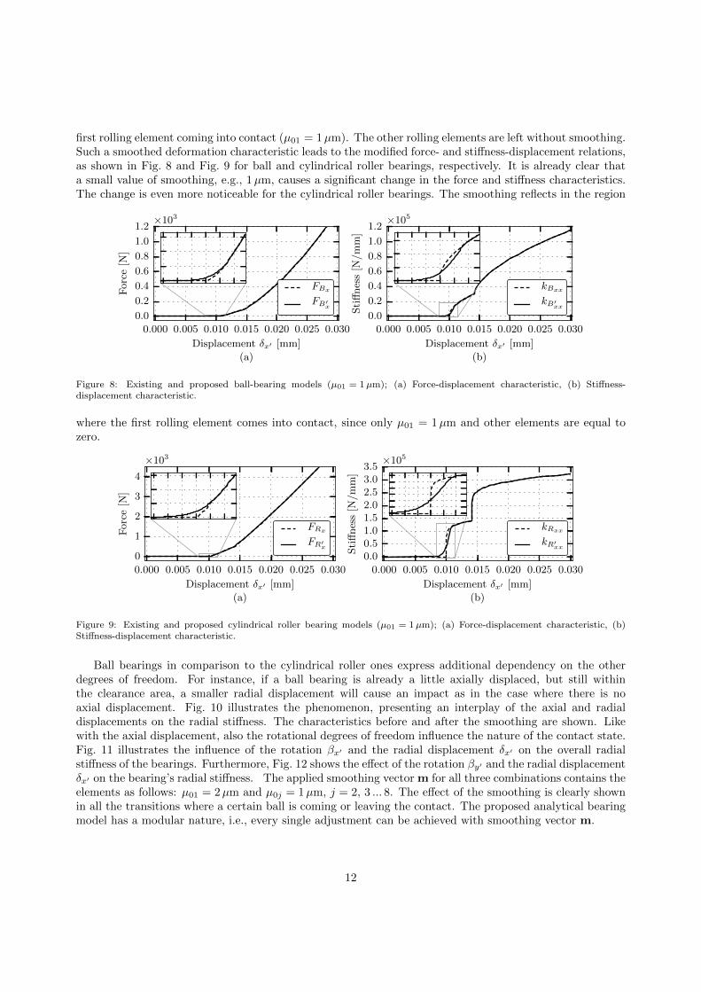
first rolling element coming into contact (µ01 = 1µm). The other rolling elements are left without smoothing.Such a smoothed deformation characteristic leads to the modified force- and stiffness-displacement relations,as shown in Fig. 8 and Fig. 9 for ball and cylindrical roller bearings, respectively. It is already clear thata small value of smoothing, e.g., 1µm, causes a significant change in the force and stiffness characteristics.The change is even more noticeable for the cylindrical roller bearings. The smoothing reflects in the region

0.000 0.005 0.010 0.015 0.020 0.025 0.030

Displacement δx′ [mm]

(a)

0.0

0.2

0.4

0.6

0.8

1.0

1.2

Forc

e[N

]

×103

FBxFB′x

0.000 0.005 0.010 0.015 0.020 0.025 0.030

Displacement δx′ [mm]

(b)

0.0

0.2

0.4

0.6

0.8

1.0

1.2

Sti

ffnes

s[N/m

m]

×105

kBxxkB′xx

Figure 8: Existing and proposed ball-bearing models (µ01 = 1µm); (a) Force-displacement characteristic, (b) Stiffness-displacement characteristic.

where the first rolling element comes into contact, since only µ01 = 1µm and other elements are equal tozero.

0.000 0.005 0.010 0.015 0.020 0.025 0.030

Displacement δx′ [mm]

(a)

0

1

2

3

4

Forc

e[N

]

×103

FRxFR′x

0.000 0.005 0.010 0.015 0.020 0.025 0.030

Displacement δx′ [mm]

(b)

0.00.51.01.52.02.53.03.5

Sti

ffnes

s[N/m

m]

×105

kRxxkR′xx

Figure 9: Existing and proposed cylindrical roller bearing models (µ01 = 1µm); (a) Force-displacement characteristic, (b)Stiffness-displacement characteristic.

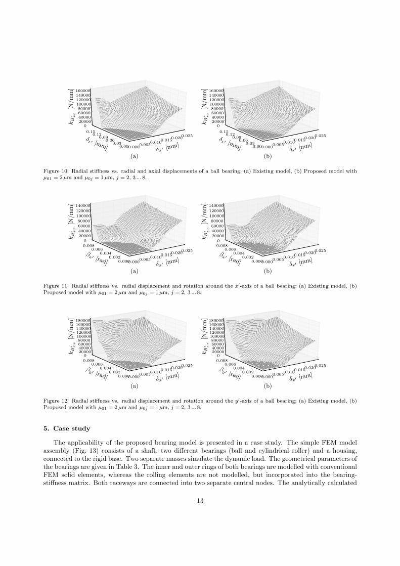
Ball bearings in comparison to the cylindrical roller ones express additional dependency on the otherdegrees of freedom. For instance, if a ball bearing is already a little axially displaced, but still withinthe clearance area, a smaller radial displacement will cause an impact as in the case where there is noaxial displacement. Fig. 10 illustrates the phenomenon, presenting an interplay of the axial and radialdisplacements on the radial stiffness. The characteristics before and after the smoothing are shown. Likewith the axial displacement, also the rotational degrees of freedom influence the nature of the contact state.Fig. 11 illustrates the influence of the rotation βx′ and the radial displacement δx′ on the overall radialstiffness of the bearings. Furthermore, Fig. 12 shows the effect of the rotation βy′ and the radial displacementδx′ on the bearing’s radial stiffness. The applied smoothing vector m for all three combinations contains theelements as follows: µ01 = 2µm and µ0j = 1µm, j = 2, 3 ... 8. The effect of the smoothing is clearly shownin all the transitions where a certain ball is coming or leaving the contact. The proposed analytical bearingmodel has a modular nature, i.e., every single adjustment can be achieved with smoothing vector m.

12

δx′ [mm]0.0000.005

0.0100.015

0.0200.025

δz ′ [mm] 0.000.03

0.060.09

0.120.15

kB′ xx

[N/m

m]

020000400006000080000

100000120000140000160000

δx′ [mm]0.0000.005

0.0100.015

0.0200.025

δz ′ [mm] 0.000.03

0.060.09

0.120.15

kB′ xx

[N/m

m]

020000400006000080000

100000120000140000160000

(a) (b)

Figure 10: Radial stiffness vs. radial and axial displacements of a ball bearing; (a) Existing model, (b) Proposed model withµ01 = 2µm and µ0j = 1µm, j = 2, 3 ... 8.

δx′ [mm]0.0000.005

0.0100.015

0.0200.025

βx ′ [rad] 0.000

0.0020.004

0.0060.008

kB′ xx

[N/m

m]

020000400006000080000

100000

120000

140000

δx′ [mm]0.0000.005

0.0100.015

0.0200.025

βx ′ [rad] 0.000

0.0020.004

0.0060.008

kB′ xx

[N/m

m]

020000400006000080000

100000

120000

140000

(a) (b)

Figure 11: Radial stiffness vs. radial displacement and rotation around the x′-axis of a ball bearing; (a) Existing model, (b)Proposed model with µ01 = 2µm and µ0j = 1µm, j = 2, 3 ... 8.

δx′ [mm]0.0000.005

0.0100.015

0.0200.025

βy ′ [rad] 0.000

0.0020.004

0.0060.008

kB′ xx

[N/m

m]

020000400006000080000

100000120000140000160000180000

δx′ [mm]0.0000.005

0.0100.015

0.0200.025

βy ′ [rad] 0.000

0.0020.004

0.0060.008

kB′ xx

[N/m

m]

020000400006000080000

100000120000140000160000180000

(a) (b)

Figure 12: Radial stiffness vs. radial displacement and rotation around the y′-axis of a ball bearing; (a) Existing model, (b)Proposed model with µ01 = 2µm and µ0j = 1µm, j = 2, 3 ... 8.

5. Case study

The applicability of the proposed bearing model is presented in a case study. The simple FEM modelassembly (Fig. 13) consists of a shaft, two different bearings (ball and cylindrical roller) and a housing,connected to the rigid base. Two separate masses simulate the dynamic load. The geometrical parameters ofthe bearings are given in Table 3. The inner and outer rings of both bearings are modelled with conventionalFEM solid elements, whereas the rolling elements are not modelled, but incorporated into the bearing-stiffness matrix. Both raceways are connected into two separate central nodes. The analytically calculated

13

Figure 13: Schematically presented FEM model assembly used for the case study.

Table 3: Properties of the ball and cylindrical roller bearings for the presented case study.

type code d [mm] D [mm] rc [µm] z rb [mm] leff [mm]

ball 6306 30 72 20 8 6 /roler N306 30 72 45 12 / 11

nonlinear bearing-stiffness matrix is prescribed between both central nodes, as demonstrated in Fig. 14. The

Figure 14: A bearing in the FEM model (black – outer ring, grey – inner ring); (a) Spider elements connecting both raceways,(b) Bearing-stiffness matrix prescribed between the central nodes.

geometrical and material properties of the assembly are given in Table 4. Furthermore the mass momentsof inertia are given in Table 5.

Table 4: Geometrical and material properties for the FEM model.

ms [kg] mh [kg] m1 [kg] m2 [kg] r1 [mm] r2 [mm] Lb [mm] Lm [mm] k [N/mm]

18.0 34.4 0.1 0.05 241 241 100 356 9

Table 5: Mass moments of inertia for the FEM model.

Ixx [kg mm2] Iyy [kg mm2] Izz [kg mm2] Ixy [kg mm2] Iyz [kg mm2] Izx [kg mm2]

shaft 703867 703840 891556 0 -3085 0housing 3305360 1426527 3076361 346075 952903 136095

The aim of our case study is to present the time response during the system’s run-up. The shaft(and eccentric masses), together with both bearing’s inner rings and associated spider elements rotate by

14

prescribed movement. In every time step the displacements and rotations between both central nodes ofeach bearing are calculated (displacement vector qb). Based on qb the bearing stiffness is provided. Theoriginal and the proposed bearing models are utilized. For the latter we prescribe µ01 = 2µm, whereas theother elements of the smoothing vector are equal to zero. It is important to note that µ01 has, in general,the greatest influence on the performance of the calculation. The shaft is governed by a constant angularacceleration ω = 0.8 rev/s

2, starting with ω = 0. The damping ratio used in the FEM model is equal to

0.1 and the numerical method employed for the time integration is Runge-Kutta-Fehlberg. Two differentregions will be presented, i.e., the initial stage of run-up and the region near the system’s resonance.

5.1. Initial stage of run-up

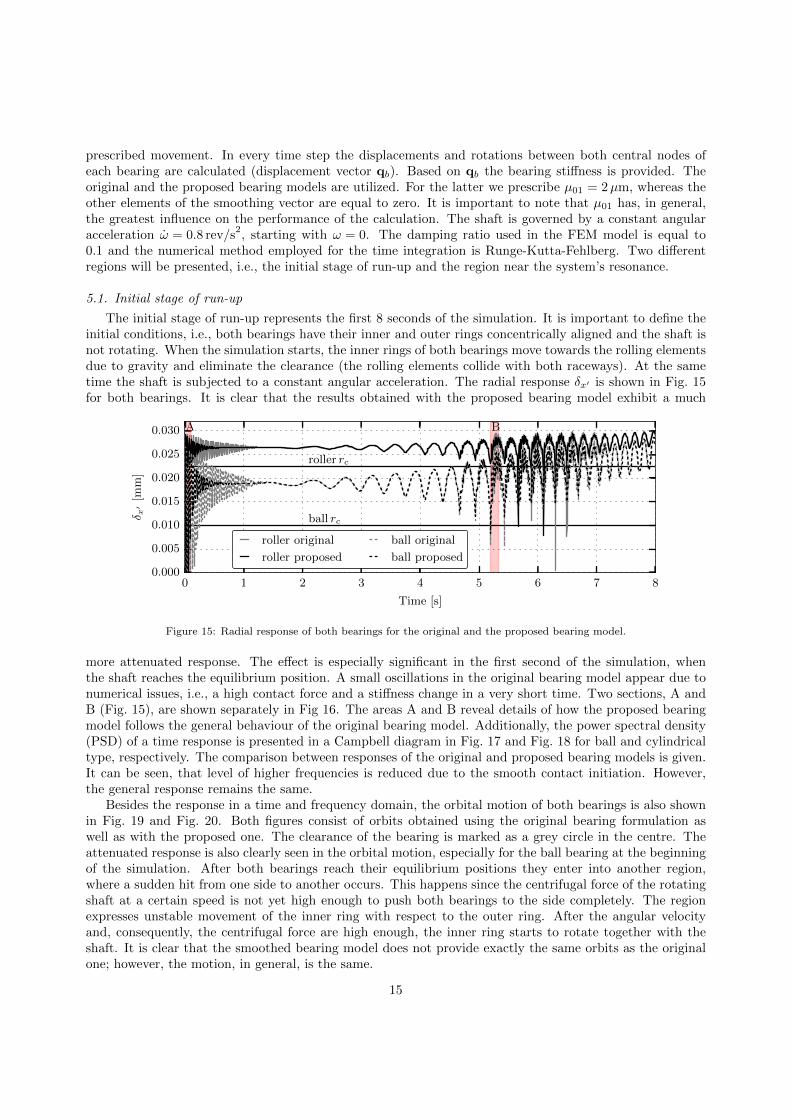
The initial stage of run-up represents the first 8 seconds of the simulation. It is important to define theinitial conditions, i.e., both bearings have their inner and outer rings concentrically aligned and the shaft isnot rotating. When the simulation starts, the inner rings of both bearings move towards the rolling elementsdue to gravity and eliminate the clearance (the rolling elements collide with both raceways). At the sametime the shaft is subjected to a constant angular acceleration. The radial response δx′ is shown in Fig. 15for both bearings. It is clear that the results obtained with the proposed bearing model exhibit a much

0 1 2 3 4 5 6 7 8

Time [s]

0.000

0.005

0.010

0.015

0.020

0.025

0.030

δ x′

[mm

]

A B

ball rc

roller rc

roller original

roller proposed

ball original

ball proposed

Figure 15: Radial response of both bearings for the original and the proposed bearing model.

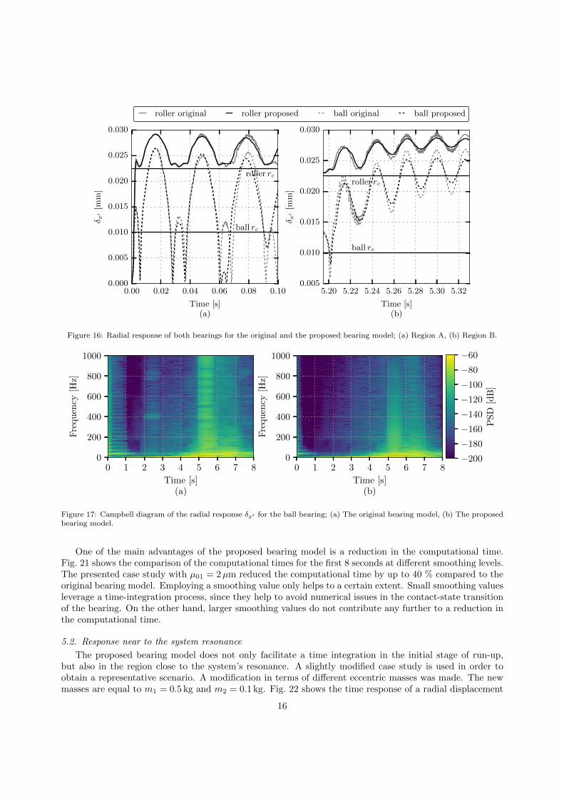
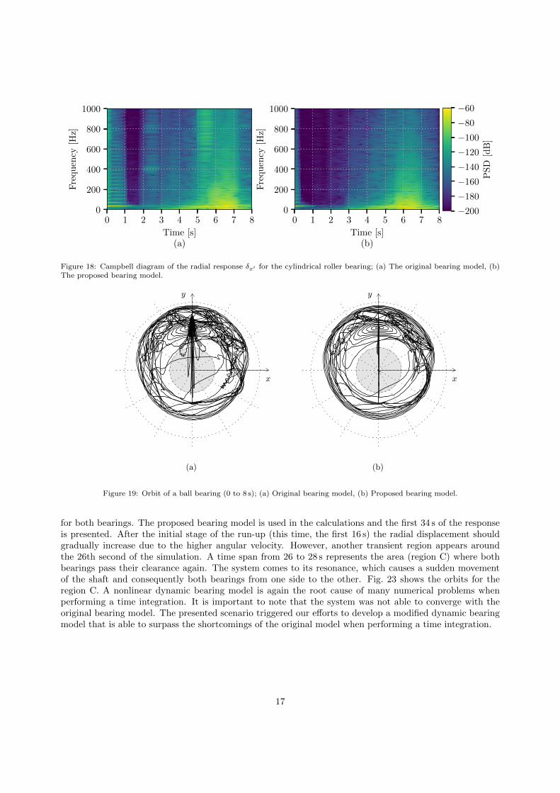
more attenuated response. The effect is especially significant in the first second of the simulation, whenthe shaft reaches the equilibrium position. A small oscillations in the original bearing model appear due tonumerical issues, i.e., a high contact force and a stiffness change in a very short time. Two sections, A andB (Fig. 15), are shown separately in Fig 16. The areas A and B reveal details of how the proposed bearingmodel follows the general behaviour of the original bearing model. Additionally, the power spectral density(PSD) of a time response is presented in a Campbell diagram in Fig. 17 and Fig. 18 for ball and cylindricaltype, respectively. The comparison between responses of the original and proposed bearing models is given.It can be seen, that level of higher frequencies is reduced due to the smooth contact initiation. However,the general response remains the same.

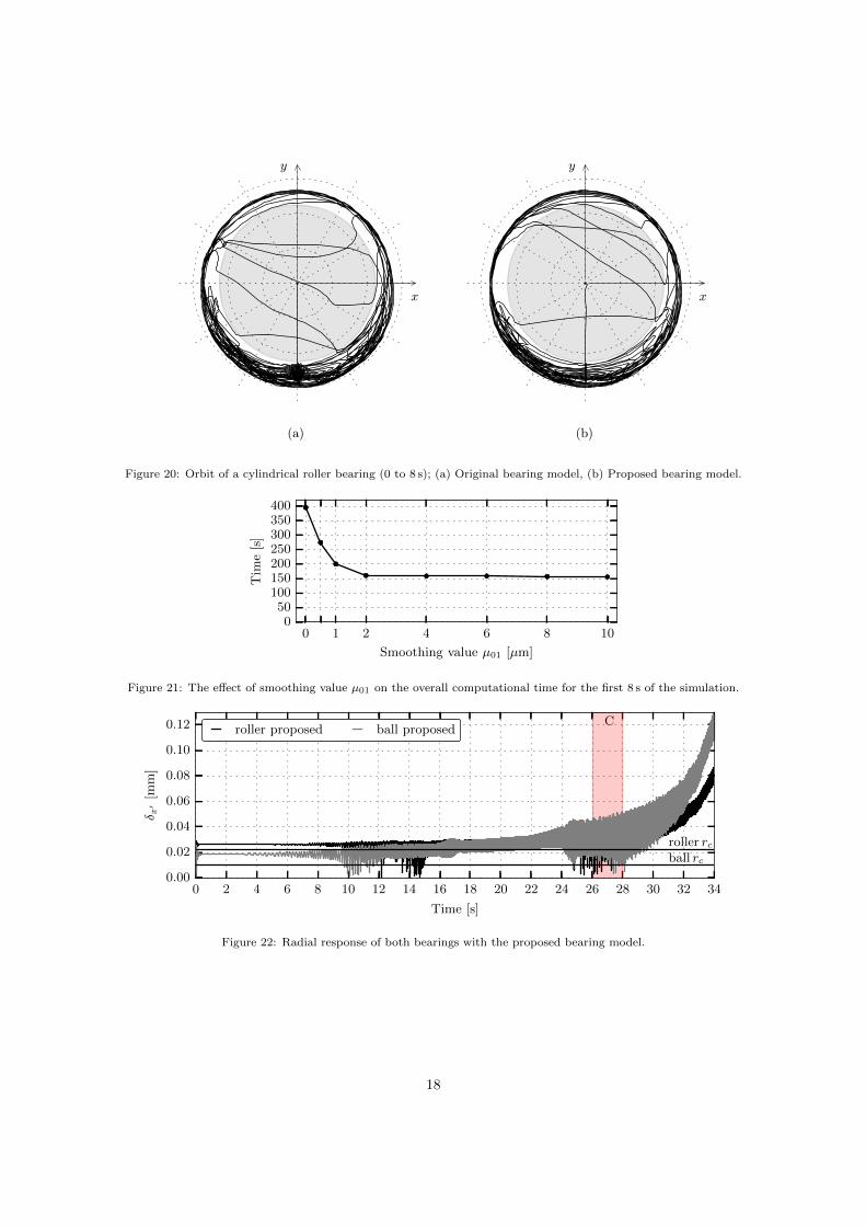
Besides the response in a time and frequency domain, the orbital motion of both bearings is also shownin Fig. 19 and Fig. 20. Both figures consist of orbits obtained using the original bearing formulation aswell as with the proposed one. The clearance of the bearing is marked as a grey circle in the centre. Theattenuated response is also clearly seen in the orbital motion, especially for the ball bearing at the beginningof the simulation. After both bearings reach their equilibrium positions they enter into another region,where a sudden hit from one side to another occurs. This happens since the centrifugal force of the rotatingshaft at a certain speed is not yet high enough to push both bearings to the side completely. The regionexpresses unstable movement of the inner ring with respect to the outer ring. After the angular velocityand, consequently, the centrifugal force are high enough, the inner ring starts to rotate together with theshaft. It is clear that the smoothed bearing model does not provide exactly the same orbits as the originalone; however, the motion, in general, is the same.

15

0.00 0.02 0.04 0.06 0.08 0.10

Time [s](a)

0.000

0.005

0.010

0.015

0.020

0.025

0.030

δ x′

[mm

]

ball rc

roller rc

5.20 5.22 5.24 5.26 5.28 5.30 5.32

Time [s](b)

0.005

0.010

0.015

0.020

0.025

0.030

δ x′

[mm

]

ball rc

roller rc

roller original roller proposed ball original ball proposed

Figure 16: Radial response of both bearings for the original and the proposed bearing model; (a) Region A, (b) Region B.

0 1 2 3 4 5 6 7 8

Time [s](a)

0

200

400

600

800

1000

Fre

qu

ency

[Hz]

0 1 2 3 4 5 6 7 8

Time [s](b)

0

200

400

600

800

1000

Fre

qu

ency

[Hz]

−200

−180

−160

−140

−120

−100

−80

−60

PS

D[d

B]

Figure 17: Campbell diagram of the radial response δx′ for the ball bearing; (a) The original bearing model, (b) The proposedbearing model.

One of the main advantages of the proposed bearing model is a reduction in the computational time.Fig. 21 shows the comparison of the computational times for the first 8 seconds at different smoothing levels.The presented case study with µ01 = 2µm reduced the computational time by up to 40 % compared to theoriginal bearing model. Employing a smoothing value only helps to a certain extent. Small smoothing valuesleverage a time-integration process, since they help to avoid numerical issues in the contact-state transitionof the bearing. On the other hand, larger smoothing values do not contribute any further to a reduction inthe computational time.

5.2. Response near to the system resonance

The proposed bearing model does not only facilitate a time integration in the initial stage of run-up,but also in the region close to the system’s resonance. A slightly modified case study is used in order toobtain a representative scenario. A modification in terms of different eccentric masses was made. The newmasses are equal to m1 = 0.5 kg and m2 = 0.1 kg. Fig. 22 shows the time response of a radial displacement

16

0 1 2 3 4 5 6 7 8

Time [s](a)

0

200

400

600

800

1000

Fre

qu

ency

[Hz]

0 1 2 3 4 5 6 7 8

Time [s](b)

0

200

400

600

800

1000

Fre

qu

ency

[Hz]

−200

−180

−160

−140

−120

−100

−80

−60

PS

D[d

B]

Figure 18: Campbell diagram of the radial response δx′ for the cylindrical roller bearing; (a) The original bearing model, (b)The proposed bearing model.

x

y

x

y

(a) (b)

Figure 19: Orbit of a ball bearing (0 to 8 s); (a) Original bearing model, (b) Proposed bearing model.

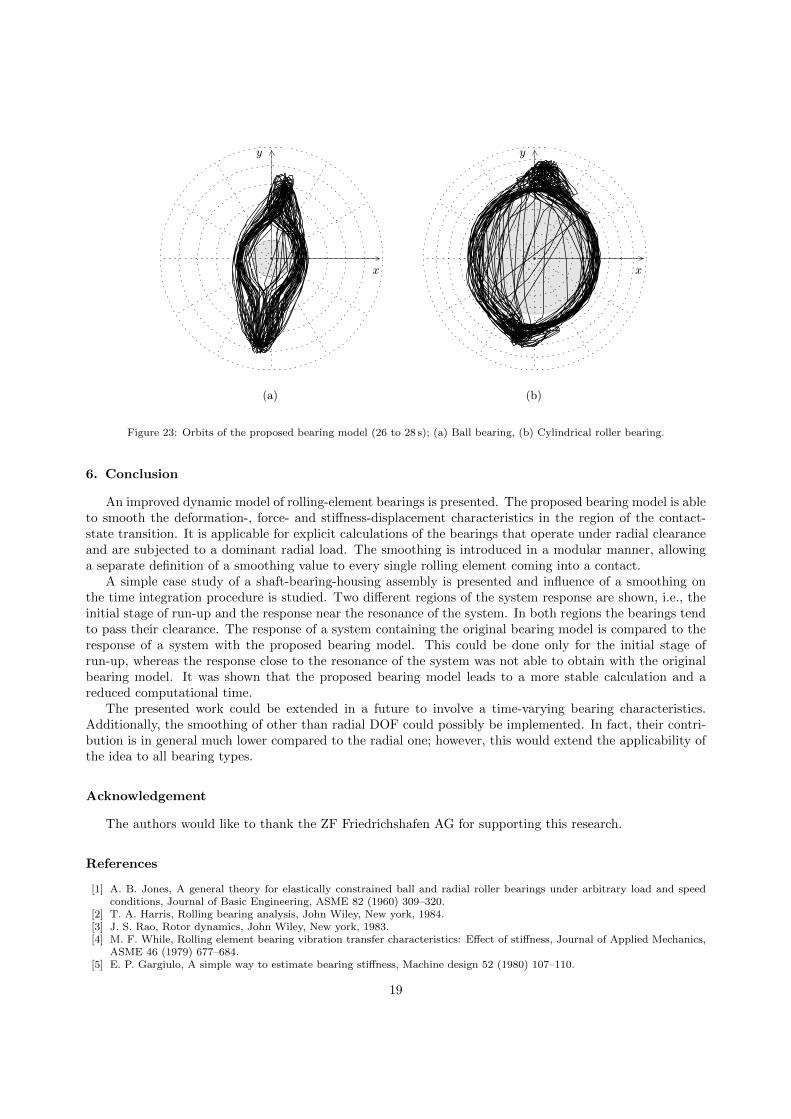
for both bearings. The proposed bearing model is used in the calculations and the first 34 s of the responseis presented. After the initial stage of the run-up (this time, the first 16 s) the radial displacement shouldgradually increase due to the higher angular velocity. However, another transient region appears aroundthe 26th second of the simulation. A time span from 26 to 28 s represents the area (region C) where bothbearings pass their clearance again. The system comes to its resonance, which causes a sudden movementof the shaft and consequently both bearings from one side to the other. Fig. 23 shows the orbits for theregion C. A nonlinear dynamic bearing model is again the root cause of many numerical problems whenperforming a time integration. It is important to note that the system was not able to converge with theoriginal bearing model. The presented scenario triggered our efforts to develop a modified dynamic bearingmodel that is able to surpass the shortcomings of the original model when performing a time integration.

17

x

y

x

y

(a) (b)

Figure 20: Orbit of a cylindrical roller bearing (0 to 8 s); (a) Original bearing model, (b) Proposed bearing model.

0 1 2 4 6 8 10

Smoothing value µ01 [µm]

050

100150200250300350400

Tim

e[s

]

Figure 21: The effect of smoothing value µ01 on the overall computational time for the first 8 s of the simulation.

0 2 4 6 8 10 12 14 16 18 20 22 24 26 28 30 32 34

Time [s]

0.00

0.02

0.04

0.06

0.08

0.10

0.12

δ x′

[mm

]

C

ball rc

roller rc

roller proposed ball proposed

Figure 22: Radial response of both bearings with the proposed bearing model.

18

x

y

x

y

(a) (b)

Figure 23: Orbits of the proposed bearing model (26 to 28 s); (a) Ball bearing, (b) Cylindrical roller bearing.

6. Conclusion

An improved dynamic model of rolling-element bearings is presented. The proposed bearing model is ableto smooth the deformation-, force- and stiffness-displacement characteristics in the region of the contact-state transition. It is applicable for explicit calculations of the bearings that operate under radial clearanceand are subjected to a dominant radial load. The smoothing is introduced in a modular manner, allowinga separate definition of a smoothing value to every single rolling element coming into a contact.

A simple case study of a shaft-bearing-housing assembly is presented and influence of a smoothing onthe time integration procedure is studied. Two different regions of the system response are shown, i.e., theinitial stage of run-up and the response near the resonance of the system. In both regions the bearings tendto pass their clearance. The response of a system containing the original bearing model is compared to theresponse of a system with the proposed bearing model. This could be done only for the initial stage ofrun-up, whereas the response close to the resonance of the system was not able to obtain with the originalbearing model. It was shown that the proposed bearing model leads to a more stable calculation and areduced computational time.

The presented work could be extended in a future to involve a time-varying bearing characteristics.Additionally, the smoothing of other than radial DOF could possibly be implemented. In fact, their contri-bution is in general much lower compared to the radial one; however, this would extend the applicability ofthe idea to all bearing types.

Acknowledgement

The authors would like to thank the ZF Friedrichshafen AG for supporting this research.

References

[1] A. B. Jones, A general theory for elastically constrained ball and radial roller bearings under arbitrary load and speedconditions, Journal of Basic Engineering, ASME 82 (1960) 309–320.

[2] T. A. Harris, Rolling bearing analysis, John Wiley, New york, 1984.[3] J. S. Rao, Rotor dynamics, John Wiley, New york, 1983.[4] M. F. While, Rolling element bearing vibration transfer characteristics: Effect of stiffness, Journal of Applied Mechanics,

ASME 46 (1979) 677–684.[5] E. P. Gargiulo, A simple way to estimate bearing stiffness, Machine design 52 (1980) 107–110.

19

[6] T. C. Lim, R. Singh, Vibration transmission through rolling element bearings, part 1: bearing stiffness formulation,Journal of Sound and Vibration 139 (2) (1990) 179–199.

[7] T. C. Lim, R. Singh, Vibration transmission through rolling element bearings, part 5: Effect of distributed contact loadon roller bearing stiffness matrix, Journal of Sound and Vibration 169 (4) (1994) 547 – 553.

[8] T. J. Royston, I. Basdogan, Vibration transmission through self-aligning (spherical) rolling element bearings: Theory andexperiment, Journal of Sound and Vibration 215 (5) (1998) 997–1014.

[9] H. V. Liew, T. C. Lim, Analysis of time-varying rolling element bearing characteristics, Journal of Sound and Vibration283 (2005) 1163–1179.

[10] A. Gunduz, R. Singh, Stiffness matrix formulation for double row angular contact ball bearings: Analytical developmentand validation, Journal of Sound and Vibration 332 (22) (2013) 5898–5916.

[11] D. S. Lee, D. H. Choi, A dynamic analysis of a flexible rotor in ball bearings with nonlinear stiffness characteristics,International Journal of Rotating Machinery 3 (1997) 73–80.

[12] X. Sheng, B. Li, Z. Wu, H. Li, Calculation of ball bearing speed-varying stiffness, Mechanisms and Machine Theory 81(2014) 166–180.

[13] Y. Guo, R. G. Parker, Stiffness matrix calculation of rolling element bearings using a finite element/contact mechanicsmodel, Mechanism and Machine Theory 51 (2012) 32–45.

[14] S. M. Vijayakar, A combined surface integral and finite element solution for a three-dimensional contact problem, Inter-national Journal for Numerical Methods in Engineering 31 (1991) 524–546.

[15] J. Zhang, B. Fang, J. Hong, S. Wan, Y. Zhu, A general model for preload calculation and stiffness analysis for combinedangular contact ball bearings, Journal of Sound and Vibration 411 (Supplement C) (2017) 435 – 449.

[16] T. C. Lim, R. Singh, Vibration transmission through rolling element bearings, part 2: system studies, Journal of Soundand Vibration 139 (2) (1990) 201–225.

[17] T. C. Lim, R. Singh, Vibration transmission through rolling element bearings, part 3: geared rotor system studies, Journalof Sound and Vibration 152 (1) (1991) 31–54.

[18] T. C. Lim, R. Singh, Vibration transmission through rolling element bearings, part 4: statistical energy analysis, Journalof Sound and Vibration 153 (1) (1992) 37–50.

[19] X. Bai, Y. Wu, K. Zhang, C. Chen, H. Yan, Radiation noise of the bearing applied to the ceramic motorized spindle basedon the sub-source decomposition method, Journal of Sound and Vibration 410 (2017) 35 – 48.

[20] P. Cermelj, M. Boltezar, An indirect approach to investigating the dynamics of a structure containing ball bearings,Journal of Sound and Vibration 276 (2004) 401–417.

[21] M. Razpotnik, T. Bischof, M. Boltezar, The influence of bearing stiffness on the vibration properties of statically overde-termined gearboxes, Journal of Sound and Vibration 351 (2015) 221–235.

[22] L.-X. Xu, Y.-G. Li, An approach for calculating the dynamic load of deep groove ball bearing joints in planar multibodysystems, Nonlinear Dynamics 70 (3) (2012) 2145–2161.

[23] L.-X. Xu, A general method for impact dynamic analysis of a planar multi-body system with a rolling ball bearing joint,Nonlinear Dynamics 78 (2) (2014) 857–879.

[24] C. A. Fonseca, I. F. Santos, H. I. Weber, Influence of unbalance levels on nonlinear dynamics of a rotor-backup rollingbearing system, Journal of Sound and Vibration 394 (Supplement C) (2017) 482 – 496.

[25] H. Wang, Q. Han, R. Luo, T. Qing, Dynamic modeling of moment wheel assemblies with nonlinear rolling bearing supports,Journal of Sound and Vibration 406 (Supplement C) (2017) 124 – 145.

[26] A. Gunduz, J. T. Dreyer, R. Singh, Effect of bearing preloads on the modal characteristics of a shat-bearing assembly:Experiments on double row angular contact ball bearings, Mechanical Systems and Signal Processing 31 (2012) 176–195.

[27] C. Bai, H. Zhang, Q. Xu, Effects of axial preload of ball bearing on the nonlinear dynamic characteristics of a rotor-bearingsystem, Nonlinear Dynamics 53 (3) (2008) 173–190.

[28] D. P. Fleming, J. V. Poplawski, Unbalance response prediction for rotors on ball bearings using speed-and load-dependentnonlinear bearing stiffness, International Journal of Rotating Machinery 2005 (1) (2005) 53–59.

[29] Z. Xia, G. Qiao, T. Zheng, W. Zhang, Nonlinear modeling and dynamic analysis of the rotor-bearing system, NonlinearDynamics 57 (4) (2009) 559–577.

[30] R. I. Leine, N. v. d. Wouw, Stability and convergence of mechanical systems with unilateral constraints, Lecture Notes inApplied and Computational Mechanics, Springer, Dordrecht, 2008.

20