A Smiling Bear in the Equity Options Market and the Cross ... · A Smiling Bear in the Equity...

A Smiling Bear in the Equity Options Market

and the Cross-section of Stock Returns

Hye Hyun Park∗, Baeho Kim†, and Hyeongsop Shim‡

(This verstion: September 20, 2016)§

ABSTRACT

We propose a measure for the convexity of an option-implied volatility curve,

IV convexity, as a forward-looking measure of risk-neutral tail-risk contribution to

the perceived variance of underlying equity returns. Using equity options data for

individual U.S.-listed stocks during 2000-2013, we find that the average realized

return differential between the lowest and highest IV convexity quintile portfolios

exceeds 1% per month, which is both economically and statistically significant on

a risk-adjusted basis. Our empirical findings indicate the contribution of informed

options trading to price discovery in terms of the realization of tail-risk aversion in

the stock market.

Keywords: Implied volatility; Convexity; Equity options; Stock returns; Predictability

JEL Classification: G12; G13; G14

∗Korea University Business School, Anam-dong, Sungbuk-Gu, Seoul 136-701, Republic of Korea, E-mail: [email protected].†Corresponding Author. Korea University Business School, Anam-dong, Sungbuk-Gu, Seoul 136-701,

Republic of Korea, Phone: +82-2-3290-2626, Fax: +82-2-922-7220, E-mail: [email protected].‡Ulsan National Institute of Science and Technology, UNIST-gil 50, Technology Management Building

701-9, Ulsan, 689-798 Republic of Korea. E-mail: [email protected].§This research was supported by the National Research Foundation of Korea Grant funded by

the Korean Government (2015S1A5A8014515), for which the authors are indebted. The authors aregrateful for helpful discussions and insightful comments to Kyounghun Bae, Ki Beom Binh, BartFrijns, Paul Geertsema, Daejin Kim, Dongcheol Kim, James A. Park, Bumjean Sohn, Sun-Joong Yoon,and participants of the 28th Australasian Finance and Banking Conference, 2015 Derivative MarketsConference, the 11th conference of Asia-Pacific Association of Derivatives. All errors are the authors’responsibility.

1. Introduction

The non-normality of stock returns has been well-documented in literature as a natural

extension of the traditional mean-variance approach to portfolio optimization.1 In general,

a rational investor’s utility is also a function of higher moments, as the investor tends to

have an aversion to negative skewness and high excess kurtosis of her asset return; see

Scott & Horvath (1980), Dittmar (2002), Guidolin & Timmermann (2008), and Kimball

(1990).2 While considerable research has subsequently examined whether the higher-

moment preference is indeed priced in the realized stock returns (e.g., Chung, Johnson &

Schill (2006); Dittmar (2002); Doan, Lin & Zurbruegg (2010); Harvey & Siddique (2000);

Kraus & Litzenberger (1976); and Smith (2007)), the higher-moment pricing effect is

embedded in equity option prices in a forward-looking manner. Specifically, the shape of

an option-implied volatility curve reveals the ex-ante higher-moment implications beyond

the standard mean-variance framework, as the curve expresses the degree of abnormality

in the option-implied distribution of the underlying stock return by inverting the standard

Black & Scholes (1973) option-pricing model.3

Although empirical research abounds in examining the risk-neutral skewness of

stock returns implied by equity option prices, the option-implied excess kurtosis has

received less attention.4 Our study attempts to fill this gap. Exploiting the fact that the

shape of an option-implied volatility curve contains information about ex-ante

higher-moment asset pricing implication, we propose a method to decompose the shape

of option-implied volatility curves into the slope and convexity components. Motivated

by stochastic volatility (SV) model and stochastic-volatility jump-diffusion (SVJ) model

specifications, we conjecture that slope and convexity of the option-implied volatility

curve contain distinct information about future stock return and convey the information

about risk-neutral skewness and the excess kurtosis of the underlying return

distributions, respectively. We confirm that the slope and convexity components (IV

slope and IV convexity hereafter) carry different information from extensive numerical

1The mean-variance approach is consistent with the maximization of expected utility if either (i)the investors’ utility functions are quadratic, or (ii) the assets’ returns are jointly normally distributed.However, a quadratic utility function may be unrealistic for practical purposes, as it exhibits increasingabsolute risk aversion, consistent with investors who reduce the dollar amount invested in risky assets astheir initial wealth increases; see Arrow (1971).

2Decreasing absolute prudence implies the kurtosis aversion according to Kimball (1990).3To better explain the positively-skewed and platokurtic preference of rational investors, prior studies

have attempted to relax the unrealistic normality assumption to capture the negatively-skewed and fat-tailed distribution of option-implied stock returns by extending the standard Black & Scholes (1973)model to stochastic volatility models and jump-diffusion models.

4There are some notable exceptions from this trend; refer to Bali, Hu & Murray (2015) and Chang,Christoffersen & Jacobs (2013) for example.

1

analyses and investigate whether the risk-neutral kurtosis, proxied by IV convexity,

predicts the cross-section of future stock returns, even after the option-implied skewness

effect is controlled.

Using equity options data for both individual U.S. listed stocks and the Standard

& Poor’s 500 (S&P500) index during 2000-2013, we study the ability of IV convexity

to predict the cross-section of future equity returns across quintile portfolios ranked by

the curvature of the option-implied volatility curve. We find a significantly negative

relationship between IV convexity and subsequent stock returns. The average return

differential between the lowest and highest IV convexity quintile portfolios exceeds 1%

per month, both economically and statistically significant on a risk-adjusted basis. The

results are robust across various definitions of the IV convexity measure. Both time series

and cross-sectional tests show that other well-known risk factors and firm characteristics

do not subsume the additional return on the zero-cost portfolio. Moreover, the predictive

power of our proposed IV convexity measure is significant for both the systematic and

idiosyncratic components of IV convexity, and the results are robust even after controlling

for the slope of the option-implied volatility curve and other known predictors based on

stock characteristics.

Where does the predictive power of IV convexity come from? Our finding is

consistent with earlier studies demonstrating the informational leading role of the

options market to the stock market. Extensive research demonstrates that equity option

markets provide informed traders with opportunities to capitalize on their information

advantage thanks to several advantages of option trading relative to stock trading.

Examples include (i) reduced trading costs (Cox & Rubinstein (1985)), (ii) the lack of

restrictions on short selling (Diamond & Verrecchia (1987)) and (iii) greater leverage

effect and built-in downside protection (Manaster & Rendleman (1982)). In this

context, Chakravarty, Gulen & Mayhew (2004) document that the option market’s

contribution to price discovery is approximately 17% on average.5 Although one may

think of the private information as being directional, information on uncertainty can

also motivate informed options trading; see Ni, Pan & Poteshman (2008) for instance.

Then, why is the relationship negative between IV convexity and the realized return of

underlying equity return in the subsequent month? We highlight that the shape of option-

implied volatility curves reveals the implication of risk-neutral higher order moments of

underlying return distributions. Given that excessive tail-risk is certainly unfavorable

to rational equity investors, the fat-tailed risk-neutral distribution incorporates ex-ante

5See also An, Ang, Bali & Cakici (2014), Chowdhry & Nanda (1991), Easley, O’Hara & Srinivas(1998), Bali & Hovakimian (2009), and Cremers & Weinbaum (2010) among others.

2

estimates of market risk premia regarding future rare events. In other words, a heavier tail

in the risk-neutral distribution is associated with a higher required return (or, equivalently,

a larger discount rate), and the informed option trading related to IV convexity predicts

a negative short-term return on the underlying stock returns as a result of price discovery

driven by an asymmetric information transmission from options traders to stock investors.

Simply put, our empirical findings indicate the contribution of informed options trading

to price discovery in terms of the realization of tail-risk aversion in the stock market. We

confirm that the predictive power of IV convexity becomes more pronounced for the firms

with stronger information asymmetry and more severe short-sale constraints, especially

during economic contraction period, and the cross-sectional predictability of IV convexity

disappears as the forecasting horizon increases.

Our study extends recent literature showing an increased interest in inter-market

inefficiency, leading to a proliferation of studies into the potential lead-lag relationship

between options and stock prices. For example, An et al. (2014) find stocks with large

innovations in at-the-money (ATM) call (put) implied volatility positively (negatively)

predict future stock returns. Xing, Zhang & Zhao (2010) propose an option-implied

volatility skew (henceforth IV smirk) measure showing its significant predictability for

the cross-section of future equity returns. Jin, Livnat & Zhang (2012) find that options

traders have superior abilities to process less anticipated information relative to equity

traders by analyzing the slope of option-implied volatility curves. Yan (2011) reports a

negative predictive relationship between the slope of the option implied volatility curve (as

a proxy of the average size of the jump in the stock price dynamics) and the future stock

return by taking the spread between the ATM call and put option-implied volatilities

(henceforth IV spread) as a measure of the slope of the implied volatility curve. Cremers

& Weinbaum (2010) argue that future stock returns can be predicted by the deviation

from the put-call parity in the equity option market, as stocks with relatively expensive

calls compared to otherwise identical puts earn approximately 50 basis points per week

more in profit than the stocks with relatively expensive puts.

This paper offers several contributions to the existing literature. First, this study

examines whether IV convexity exhibits significant predictive power for future stock

returns even after controlling for the effect of IV slope and other firm-specific

characteristics. Although recent evidence shows that the skewness component of the

risk-neutral distribution of underlying stock returns, our research is, to the best of our

knowledge, the first study that makes a sharp distinction between the 3rd and 4th

moments of equity returns implied by option prices. Specifically, we decompose the

information extracted from the shape of option-implied volatiltiy curve into separate IV

3

slope and IV convexity measures, and empirically verify that IV convexity significantly

predicts the cross section of future stock returns even after controlling for the IV slope

effect. Furthermore, IV spread measure proposed by Yan (2011) simply captures the

effect of the average jump size but not the effect of jump-size volatility in the SVJ

model framework. We extend those findings by examining how IV convexity explains

the cross-section of future stock returns to address the jump-size volatility effect.

Furthermore, this paper overcomes the potential caveat of ex-post information from past

realized returns in the previous studies on the effect of skewness (e.g., Kraus &

Litzenberger (1976); Lim (1989); Harvey & Siddique (2000)) by estimating an ex-ante

measures of skewness (IV slope) and excess kurtosis (IV convexity) from the

forward-looking option price data.6

This paper sheds new light on the relationship between the higher-moment

information from individual equity option prices and the cross-section of future stock

returns. Chang et al. (2013) investigate how market-implied skewness and kurtosis affect

the cross-section of stock returns by looking at the risk-neutral skewness and kurtosis

implied by index option prices based on the model framework proposed by Bakshi,

Kapadia & Madan (2003). However, their approach ignores the idiosyncratic

components of option-implied higher moments in stock returns.7 Our paper extends the

findings of Chang et al. (2013) by employing firm-level equity option price data, and

further decomposing IV convexity into systematic and idiosyncratic components to fully

identify the lead-lag relationship between IV convexity and the cross-section of future

stock returns.

2. Motivation

In this section, we demonstrate the asset pricing implications of our proposed IV

convexity measure. As known, an option-implied risk-neutral distribution of the

underlying stock return exhibits heavier tails than the normal distribution with the same

mean and standard deviation, in the presence of higher moments such as skewness and

excess kurtosis.8 Accordingly, information about these higher moments embedded in the

various shapes of implied volatility curves can be examined from various perspectives.

6The ex-post higher moments estimated from the realized stock returns can be biased unless the returndistribution is stationary and time-invariant; refer to Bali et al. (2015) and Chang et al. (2013).

7Yan (2011) finds that both the systematic and idiosyncratic components of IV spread are priced andthat the latter dominates the former in capturing the cross-sectional variation of future stock returns.

8Hereafter, we use kurtosis and excess kurtosis interchangeably, despite their conceptual differences.

4

Figure 1: Shape of the Implied Volatility Curves

This figure illustrates the effect of different values of skewness and excess kurtosis of underlying

asset returns on the shape of the implied volatility curve. The base parameter set is taken as (r,

σ, skewness, excess kurtosis)=(0.05, 0.3,−0.5, 1.0) where r is the risk-free rate and σ is standard

deviation, and (S0, T ) = (100, 0.5) as an illustrative example.

0.8 0.85 0.9 0.95 1 1.05 1.1 1.15 1.20.2

0.22

0.24

0.26

0.28

0.3

0.32

0.34

0.36

Moneyness (K/S)

Impl

ied

Vol

atili

ty

Skewness = −1.0Skewness = −0.75Skewness = −0.5Skewness = −0.25Skewness = 0.0

0.8 0.85 0.9 0.95 1 1.05 1.1 1.15 1.20.23

0.24

0.25

0.26

0.27

0.28

0.29

0.3

0.31

0.32

0.33

Moneyness (K/S)

Impl

ied

Vol

atili

ty

Kurtosis = 0.0Kurtosis = 0.5Kurtosis = 1.0Kurtosis = 1.5Kurtosis = 2.0

2.1. Risk-neutral Higher-order Moments

To explore the effects of risk-neutral skewness and excess kurtosis on option pricing, we

consider a geometric Levy process to model the risk-neutral dynamics of the underlying

stock price given by

St = S0eXt , (1)

where X is the return process whose increments are stationary and independent. In this

context, a natural characterization of a probability distribution is specifying its cumulants,

as we can readily expand the probability distribution function via the Gram-Charlier

expansion, a method to express a density probability distribution in terms of another

(typically Gaussian) probability distribution function using cumulant expansions.9 This

feature aids in understanding how the skewness and kurtosis of the underlying asset return

affect the shape of the option-implied volatility curves.10

Figure 1 illustrates the effect of different values of skewness and excess kurtosis on the

shape of an implied volatility curve. We can observe that a negatively skewed distribution,

ceteris paribus, leads to a steeper volatility smirk, whereas an increase in the excess

9The nth cumulant is defined as the nth coefficient of the Taylor expansion of the cumulant generatingfunction, the logarithm of the moment generating function. Intuitively, the first cumulant is the expectedvalue, and the nth cumulant corresponds to the nth central moment for n = 2 or n = 3. For n ≥ 4, thenth cumulant is the nth degree polynomial in the first n central moments.

10See Tanaka, Yamada & Watanabe (2010) for details of the application of Gram-Charlier expansionfor option pricing.

5

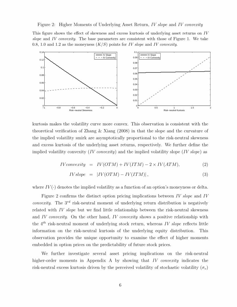
Figure 2: Higher Moments of Underlying Asset Return, IV slope and IV convexity

This figure shows the effect of skewness and excess kurtosis of underlying asset returns on IV

slope and IV convexity. The base parameters are consistent with those of Figure 1. We take

0.8, 1.0 and 1.2 as the moneyness (K/S) points for IV slope and IV convexity.

−1 −0.8 −0.6 −0.4 −0.2 00

0.02

0.04

0.06

0.08

0.1

0.12

0.14

Risk−neutral Skewness

IV SlopeIV Convexity

0 0.5 1 1.5 20

0.01

0.02

0.03

0.04

0.05

0.06

0.07

0.08

0.09

0.1

Risk−neutral Kurtosis


kurtosis makes the volatility curve more convex. This observation is consistent with the

theoretical verification of Zhang & Xiang (2008) in that the slope and the curvature of

the implied volatility smirk are asymptotically proportional to the risk-neutral skewness

and excess kurtosis of the underlying asset returns, respectively. We further define the

implied volatility convexity (IV convexity) and the implied volatility slope (IV slope) as

IV convexity = IV (OTM) + IV (ITM)− 2× IV (ATM), (2)

IV slope = |IV (OTM)− IV (ITM)| , (3)

where IV (·) denotes the implied volatility as a function of an option’s moneyness or delta.

Figure 2 confirms the distinct option pricing implications between IV slope and IV

convexity. The 3rd risk-neutral moment of underlying return distribution is negatively

related with IV slope but we find little relationship between the risk-neutral skewness

and IV convexity. On the other hand, IV convexity shows a positive relationship with

the 4th risk-neutral moment of underlying stock return, whereas IV slope reflects little

information on the risk-neutral kurtosis of the underlying equity distribution. This

observation provides the unique opportunity to examine the effect of higher moments

embedded in option prices on the predictability of future stock prices.

We further investigate several asset pricing implications on the risk-neutral

higher-order moments in Appendix A by showing that IV convexity indicates the

risk-neutral excess kurtosis driven by the perceived volatility of stochastic volatility (σv)

6

and jump volatility (σJ) of underlying asset returns. The results confirm that IV

convexity is a forward-looking measure of excess tail-risk contribution to the perceived

variance of underlying equity returns under the risk-neutral measure.

2.2. Hypothesis Development

Having observed that the convexity of an option-implied volatility curve is a

forward-looking measure of the perceived likelihood of extreme movements in the

underlying equity price, we develop our empirical research question by examining how

IV convexity is related to the cross-section of future underlying stock returns. Notice

that the aforementioned theoretical analyses are based on the perfect information flow

between options and stock markets, where expected returns are irrelevant for option

pricing and equity investors express their tail-risk aversion simultaneously when equity

option investors generate leptokurtic implied distributions of future stock returns.

In reality, however, numerous empirical studies have identified that options market

would be an ideal venue for informed trading and options market could lead stock market

in the price discovery process, as informed traders have incentives to trade in options

markets to benefit from their informational advantage. Specifically, higher risk-neutral

excess kurtosis in the options market, ceteris paribus, can be an early warning signal of

the realized tail-risk aversion in the equity market, and vice versa. As such, we expect

that a persistent predictive capability of IV convexity for future stock returns with a

negative relationship would appear to link the risk-neutral excess kurtosis of the option-

implied stock returns to tail-risk aversion of stock investors with a significant time lag.

We summarize our research questions in the following testable main hypothesis:

• Main hypothesis: A slow and one-way information transmission from options to

stock markets enables informed options traders to capitalize on their private

information on the forthcoming of ex-post tail-risk perception in the stock market.

As a result, IV convexity would appear to link the excess kurtosis of the

risk-neutral stock returns to the realization of equity investors’ tail-risk aversion

associated with a higher tail-risk premium (or, equivalently, a larger discount rate)

with a significant time lag. This delayed price discovery mechanism will show a

persistent predictive capability of IV convexity for future stock returns with a

negative relationship.

The overall goal of our empirical analysis is to examine if the IV convexity measure

can show a significant cross-sectional predictive power for future equity returns. If we

7

observe negative relationship between IV convexity and future stock return with statistical

significance, it would empirically support the existing literature demonstrating the lead-

lag relationship between the options and stock markets in terms of the realization of

delayed tail-risk premium in the stock market.

3. Empirical Analysis

This section introduces our data set and methodology to estimate option-implied

convexity in a cross-sectional manner. We test whether IV convexity has strong

predictive power for future stock returns with statistical significance. Then, we compare

the impact of IV convexity with that of option-implied volatility slope on the future

underlying stock returns in the presence of various control variables.

3.1. Data and Sample

We obtain the U.S. equity and index option data from OptionMetrics on a daily basis

from January 2000 through December 2013. As the raw data include individual equity

options in the American style, OptionMetrics applies the binomial tree model of Cox,

Ross & Rubinstein (1979) to estimate the options-implied volatility curve to account for

the possibility of an early exercise with discrete dividend payments. Employing a kernel

smoothing technique, OptionMetrics offers an option-implied volatility surface across

different option deltas and time-to-maturities. Specifically, we obtain the fitted implied

volatilities on a grid of fixed time-to-maturities, (30 days, 60 days, 90 days, 180 days,

and 360 days) and option deltas (0.2, 0.25, . . . , 0.8 for call options and -0.8, -0.75, . . . ,

-0.2 for put options), respectively. Following An et al. (2014) and Yan (2011), we then

select the options with 30-day time-to-maturity at the end of each month to examine the

predictability of IV convexity for future stock returns.

[Table 1 about here.]

Table 1 shows the summary statistics of the fitted implied volatility and fixed deltas

of the individual equity options with one month (30 days) time-to-maturity chosen at the

end of each month. We can observe a positive convexity in the option-implied volatility

curve as a function of the option’s delta in that the implied volatilities from in-the-money

(ITM) options (calls for delta of 0.55 ∼ 0.80, puts for delta of −0.80 ∼ −0.55) options

and OTM (calls for delta of 0.20 ∼ 0.45, puts for delta of −0.45 ∼ −0.20) are greater on

8

average than those near the ATM options (calls for delta of 0.50, puts for delta of −0.50).

Panel B of Table1 reports the unique number of firms by industry each year. Each firm is

assigned into one of the Fama-French 12 industries (FF1-12) classification based on its SIC

code. There are 2,900 unique firms in 2000, rising to 4,159 in 2013. We obtain daily and

monthly individual common stock (shrcd in 10 or 11) returns from the Center for Research

in Security Prices (CRSP) for stocks traded on the NYSE (exchcd=1), Amex (exchcd=2),

and NASDAQ (exchcd=3). Stocks with a price less than three dollars per share are

excluded to weed out very small or illiquid stocks and the potential extreme skewness

effect (Loughran & Ritter (1996)). Accounting data is obtained from Compustat. We

obtain both daily and monthly data for each factor from Kenneth R. French’s website.11

3.2. Variables and portfolio formation

We adopt IV convexity as a risk-neutral proxy for the option-implied tail-risk perception

on the underlying stock returns over the life of option. Throughout this paper, we propose

our main measure of IV convexity defined as

IV convexity = IVput(−0.2) + IVput(−0.8)− 2× IVcall(0.5), (4)

where IVput(∆) and IVcall(∆) refer to the fitted put and call option-implied volatilities

with one month (30 days) to expiration, and ∆ is each options’ delta.12 Note that the

violation of put-call parity is commonly observed in practice, as the parity does not

account for potential market frictions and there is an early exercise possibility for deep

in-the-money American put options; e.g., Yan (2011) and Cremers & Weinbaum (2010)

find that the spread between put- and call-implied volatilities can predict the cross-section

of unerlying stock returns.

As shown in (4), IV convexity is defined as the sum of OTM and ITM put implied

volatilities less double the ATM call implied volatility.13 The rationale is that those who

have private information on the (forthcoming) widespread tail-risk aversion would buy a

cheap deep-OTM put option as a protection against the potential decrease in the stock

return for hedging purposes or buy a deep-ITM put option for taking its early exercise

premium as a leverage to grab a quick profit for speculative purposes to capitalize on

11http://mba.tuck.dartmouth.edu/pages/faculty/ken.french/data_library.html.12Delta is commonly used as the industry practice of measuring moneyness, as an option’s delta is

sensitive to the option’s intrinsic value and time-value at the same time. Our results are robust acrossdifferent measures of moneyness, as we consider short-term maturity options in our analysis.

13See Section 3.4 for alternative measures of IV convexity.

9

http://mba.tuck.dartmouth.edu/pages/faculty/ken.french/data_library.html

private information.14 For the same reasoning, an informed investor who anticipate

heavier tail-risk aversion prevailing in the stock market would sell call options. We

subtract double the implied volatility of the ATM call option, which is generally the

most frequently traded option best reflecting market participants’ sentiment regarding

the firm’s future condition.

We also consider other measures related to the shape of option-implied volatility

curve. Specifically, option-implied volatility level and slope, denoted by IV level and IV

slope respectively, are defined as

IV level = 0.5× [IVput(−0.5) + IVcall(0.5)] , (5)

IV slope = IVput(−0.2)− IVput(−0.8), (6)

respectively. This decomposition enables us to investigate whether the IV slope and

IV convexity actually have distinct impacts on a cross-section of future stock returns,

thereby to check whether IV convexity carries extra predictability of future stock returns

controlling for return predictability of IV slope. Furthermore, we define IV spread as

IV spread = IVput(−0.5)− IVcall(0.5), (7)

which is proposed by Yan (2011), who argues that the IV spread mainly reflects the

contribution of 3rd moments of return distributions driven by the mean jump size in the

price dynamics. Next, motivated by Xing et al. (2010), we define IV smirk as the difference

between the implied volatility of the OTM put options and the ATM call options on the

same stock. If there are more than one record of OTM put or ATM call options for a

certain stock on the same day, we take the OTM put option with the moneyness (= K/S)

closest to 0.95 and the ATM call option with its moneyness (= K/S) closest to 1.15

14Although an ITM put option is costly, its demand can increase under strong short-sale constraints ofunderlying stocks with pessimistic tail-risk perception, as a severe short-selling constraint would make itmore expensive to capitalize on their negative private information in the equity market, where ITM putoptions would be rational alternatives. Recall that the delta of a deep-ITM American put option is closeto -1 owing to the possibility of early exercise.

15Xing et al. (2010) estimate IV smirk from the implied volatilities of options data, for which we applythe following filters to minimize the impact of recording errors. Following their methodology, we eliminatethe prices that violate no-arbitrage condition by using call data only when the call option prices fall insideof the interval (St −Dt,T −Ke−rt,T , S) and use put data only when the put option prices remain insideof the interval (Ke−rt,T − (St −Dt,T ), S), where S is the price of underlying stock, K is the strike priceof options, r is risk-free rate and D is the dollar dividend and T is the expiration time. We remove theoptions from the sample if their average of best bid price and best ask price is higher than $0.125, thebid price is equal to zero, or the ask price is lower than the bid price. We include the option contractwith positive open interest and non-missing volume data. The time-to-maturity of the options must bebetween 10-60 days and the implied volatility of the option should be between 3% and 200%.

10

Taking advantage of both equity options and index options data, we can disentangle

IV convexity into systematic and the idiosyncratic components. For this purpose, we run

the time series regression each month using the S&P500 index options with 30-day time-to

maturity as a benchmark for the market along with individual equity options at the end

of each month given by

IV convexityi,k = αi + βi × IV convexityS&P500,k + εi,k, (8)

where t − 30 ≤ k ≤ t − 1 on a daily basis. We define the fitted values and residual

terms as the systematic component of IV convexity (convexitysys) and the idiosyncratic

component of IV convexity (convexityidio), respectively.


At the end of each month, we compute the cross-sectional IV level, IV slope, IV

convexity, IV smirk, and IV spread measures from 30-day time-to-maturity options. Panel

A of Table 2 shows the descriptive statistics for each implied volatility measure computed

at the end of each month using 30-day time-to-maturity options. As for the average values

for each of variable, IV level has 0.4739, IV slope for 0.0423, IV spread for 0.0090, IV

smirk for 0.0687, and IV convexity for 0.0952, respectively. The standard deviation of

IV convexity is 0.2774, and 0.1703 for convexitysys, 0.2235 for convexityidio, respectively.

Panel B of Table 2 reports the descriptive statistics of firm characteristics and asset pricing

factors.16

3.3. Predictive power of IV convexity

We now report our empirical results regarding the predictive power of IV convexity for

the cross-section of future underlying stock returns. When constructing a single sorted IV

convexity portfolio, we sort all stocks at the end of each month based on the IV convexity

and match with the subsequent monthly stock returns. The IV convexity portfolios are

rebalanced every month.


Panel A of Table 3 reports the means and standard deviations of the five IV convexity

quintile portfolios and average monthly portfolio returns of both equal-weighted (EW) and

16See Appendix B for our variable definitions of firm characteristics (Size, BTM) and asset pricingfactors (Market β, MOM, REV, ILLIQ and Coskew).

11

value-weighted (VW) portfolios over the entire sample period. To examine the relationship

between IV convexity and future stock returns, we form five portfolios according to the

IV convexity value at the end of each month. Quintile 1 is composed of stocks with the

lowest IV convexity, while Quintile 5 is composed of stocks with the highest IV convexity.

These portfolios are rebalanced every month, and assumed to be held for the subsequent

one-month period. As shown, the average EW portfolio return monotonically decreases

from 0.0208 for the lowest quintile portfolio Q1 to 0.0074 for the highest quintile portfolio

Q5. The average monthly return of the arbitrage portfolio buying the lowest IV convexity

portfolio Q1 and selling highest IV convexity portfolio Q5 is significantly positive (0.0134

with t-statistics of 7.87). The average VW portfolio returns exhibit a similar decreasing

pattern from Q1 (0.0136) to Q5 (0.0023), and the return of zero-investment portfolio

(Q1-Q5) is significantly positive (0.0113 with t-statistics of 5.08).

Panel B and C of Table 3 show the average monthly returns of quintile portfolios

sorted by IV spread and IV smirk, respectively. The EW portfolios sorted by IV spread

show that their EW portfolio returns decrease monotonically from 0.0145 for quintile

portfolio Q1 to 0.0013 for quintile portfolio Q5, where the average return difference

between Q1 and Q5 amounts to 0.0131 with t-statistics of 7.31 and similar patterns are

observed with VW portfolios sorted by IV spread. These results certainly confirm the

empirical finding of Yan (2011) in that low IV spread stocks outperform high IV spread

stocks. In a similar vein, we find from Panel C that the average returns of quintile

portfolios sorted by IV smirk are decreasing in IV smirk, and the returns of

zero-investment portfolios (Q1-Q5) are all positive and statistically significant for both

the EW and VW portfolios, consistent with Xing, Zhang and Zhao (2010) in that there

exists a negative predictive relationship between IV smirk and future stock return.

Left panel of Figure 3 shows the monthly average IV convexity value for each quintile

portfolio, while Right panel plots the monthly average return of the arbitrage portfolio

formed by taking long position in the lowest quintile and short position in the highest

quintile portfolios (Q1-Q5). The time-varying average monthly returns of the long-short

portfolio are mostly positive, confirming the results reported in Table 3.

3.4. Alternative IV convexity measures

We next consider alternative measures of options-implied volatility convexity than ours

given by (4). We first explore various IV convexity measures by varying ITM and OTM

points of put options. Panel A of Table 4 reports descriptive statistics for average portfolio

returns based on the main IV convexity measure given by (4) estimated with various delta

12

Figure 3: Average IV convexity and Quintile Portfolio Returns

This figure shows the time-series behavior of the average IV convexity of the quintile portfolios

(Left panel) and the monthly average returns of the long-short portfolios Q1-Q5 (Right panel)

from Jan 2000 to Dec 2013 on a monthly basis.

Jan-00 01-Sep 03-May 05-Jan 06-Sep 08-May 10-Jan 11-Sep 13-May-0.5

0

0.5

1

1.5

Q1Q2Q3Q4Q5

Feb-00 01-Oct 03-Jun 05-Feb 06-Oct 08-Jun 10-Feb 11-Oct 13-Jun-0.05

0

0.05

0.1

0.15

Q1-Q5

points. The decreasing patterns in portfolio returns are still observed across different delta

points and arbitrage portfolio (Q1-Q5) returns are significantly positive for both the

equal-weighted and value-weighted portfolio returns. This result confirms the negative

relationship between IV convexity and future stock returns whatever delta points of put

options we use to compute convexity.


Next, we construct various alternative measures of IV convexity, denoted by

IV convexity(·), between calls and puts given by

IV convexity(II) = IVput(−0.2) + IVput(−0.8)− 2× IVput(−0.5), (9)

IV convexity(III) = IVcall(0.2) + IVcall(0.8)− 2× IVcall(0.5), (10)

IV convexity(IV ) =IV convexity(II) + IV convexity(III)

2, (11)

IV convexity(V ) = IVput(−0.2) + IVcall(0.2)− 2× IVput(−0.5), (12)

IV convexity(V I) = IVput(−0.2) + IVcall(0.2)− 2× IVcall(0.5). (13)

As a benchmark, we first construct a put-based convexity measure, IV convexity(II), and

a call-based measure, IV convexity(III). Then, we define IV convexity(IV ) as the average

of IV convexity(II) and IV convexity(III) to incorporate comprehensive implied volatility

information from call and put options. Further, IV convexity(V ) and IV convexity(V I) are

13

constructed by the sum of OTM option-implied volatilities less the ATM option-implied

volatility. The rationale behind them is the fact that OTM put (call) options are generally

more liquid than the ITM call (put) options at the same strike prices.

We then construct a set of single-sorted quintile portfolios (from Q1 to Q5) by

sorting all stocks at the end of each month based on each of the alternative IV convexity

measures and match with the subsequent monthly stock returns. Quintile 1 is composed

of stocks with the lowest IV convexity(·) while Quintile 5 is composed of stocks with the

highest IV convexity(·). That is, at the end of each month, all firms are assigned to one

of five portfolio groups based on alternative options implied convexity. These portfolios

are equally weighted, rebalanced every month, and assumed to be held for the

subsequent one-month period. This process is repeated in every month. Panel B of

Table 4 reports the descriptive statistics of the average portfolio returns sorted by

alternative measures of IV convexity given by (4)-(13). Our empirical results show that

the alternative IV convexity measures generally produce a monotone decreasing pattern

of the average quintile portfolio returns, and the realized returns of the arbitrage

portfolio (Q1-Q5) across different definitions of IV convexity remain positive with

statistical significance.17 This result confirms our main hypotheses in that the negative

relationship between IV convexity and future stock returns are robust and consistent

across different definitions of IV convexity.

3.5. Controlling Firm-specific Factors

We investigate whether the positive arbitrage portfolio returns (Q1-Q5) are still significant

even after controlling for firm-specific equity risk factors. Accordingly, we test whether a

set of representative firm characteristics crowd out the negative relationship between IV

convexity and stock returns. To examine whether the relationship between IV convexity

and stock returns disappear after controlling for the firm characteristics, we double-sort

all stocks following Fama & French (1992). Specifically, all stocks are sorted into five

quintiles by ranking on standard equity risk factors and then sorting within each quintile

into five quintiles according to IV convexity.


We first adopt the suggestion of Fama & French (1993) in that firm size,

book-to-market ratio, and Market β are regarded as the three main firm characteristic

17The mean arbitrage portfolio returns are significantly positive at 5% confidence level across differentmeasures of IV convexity except for the case of IV convexity(II) at 10% level of confidence.

14

factors of stock returns. Table 5 reports the average monthly returns of the 25 (5 × 5)

portfolios sorted first by firm characteristic risks (firm size, book-to-market ratio, and

Market β) and then by IV convexity and average monthly returns of the long-short

arbitrage portfolios (Q1-Q5). We can observe that the average monthly portfolio returns

generally decline as the average firm-size increases. As shown in the results from

double-sorting using firm-size and IV convexity, we find that the returns of the IV

convexity quintile portfolios are still decreasing in IV convexity in most size quintiles,

and the return of all zero-investment portfolios (Q1-Q5) in size quintiles are all positive

and statistically significant. In particular, the positive difference in the smallest quintile

is the largest (0.0187) compared to the other size quintile portfolios.

The two-way cuts on book-to-market and IV convexity show that the higher book-

to-market portfolio gets more returns compared to the lower book-to-market portfolios

in each IV convexity quintile. The decreasing patterns in IV convexity portfolio returns

remain even after controlling the systematic compensation drawn from the book-to-market

factor. Note that the overall zero-cost portfolios formed by long Q1 and short Q5 are also

positive and statistically significant: 0.0097 (t-statistic of 4.82) for B1 (BTM quintile 1),

0.0121 (t-statistic of 5.76) for B2, 0.0108 (t-statistic of 5.42) for B3, 0.0134 (t-statistic of

5.67) for B4, and 0.0177 (t-statistic of 5.19) for B5.

When sorting the 25 portfolios first by Market β and then by IV convexity, the

negative relationship between IV convexity and stock return persists, implying that this

decreasing pattern cannot be explained by Market β. Note that the average monthly

portfolio returns generally increase as the average Market β rises.

We also consider the other four pricing factors of (i) the momentum effect documented

by Jegadeesh & Titman (1993), (ii) the short-term reversal suggested by Jegadeesh (1990)

and Lehmann (1990), (iii) the illiquidity proposed by Amihud (2002) and (iv) co-skewness

suggested by Harvey & Siddique (2000) to examine whether the decreasing pattern of

portfolio returns in IV convexity disappears when controlling these systematic risk factors.

Stocks are first sorted into five groups based on their momentum (or reversal, illiquidity,

co-skewness) measures and then sorted by IV convexity forming 25 (5 × 5) portfolios.


Table 6 presents the returns of 25 portfolios sorted by each of four equity pricing

factors (momentum, reversal, illiquidity, co-skewness) and IV convexity. When we look

at the momentum patterns in the momentum-IV convexity portfolios, winner portfolios

consistently achieve more abnormal returns than loser portfolios except for the lowest

15

momentum-lowest IV convexity quintiles, which could be caused by using a different

sample datasets compared to that in Jegadeesh & Titman (1993). While Jegadeesh &

Titman (1993) use only stocks traded on the NYSE (exchcd=1) and Amex (exchcd=2),

we add stocks traded on the NASDAQ (exchcd=3). For the holding period strategies,

Jagadeesh and Titman (1993) adopt 3-, 6-, 9-, and 12-month holding periods, while this

study assumes that portfolios are held for one month.

Even after controlling momentum as a systematic risk, we observe that the portfolio

return differential between the lowest and highest IV convexity in each momentum

quintile remains significantly positive, indicating that IV convexity contains

economically meaningful information that cannot be explained by the momentum factor.

For the reversal-IV convexity double sorted portfolio case, there is a clear reversal

patterns in most cases when using a reversal strategy (i.e., the past winner earns higher

returns in the next month compared to past loser), though there are some distortions

in the lowest reversal-highest IV convexity quintiles. The Q1-Q5 strategy of buying and

selling stocks based on IV convexity in each reversal portfolio and holding them for one

month still earns significantly positive returns. This implies that the same results still

hold even after controlling for reversal effects.

We further incorporate the Amihud (2002) measure of illiquidity to address the role

of the liquidity premium in asset pricing. Amihud (2002) finds that the expected market

illiquidity has positive and highly significant effect on the expected stock returns, as

investors in the equity market require additional compensation for taking liquidity risk.

We examine whether the market illiquidity measure (ILLIQ) explains the higher return

on the lowest IV convexity stock portfolio (Q1) relative to the highest IV convexity

stock portfolio (Q5). The double-sorted quintile portfolios by ILLIQ andIV convexity

exhibit analogous patterns in that their average returns tend to decrease in IV

convexity. The zero-investment portfolios (Q1-Q5) based on the ILLIQ quintiles

demonstrate their significantly positive average returns across different ILLIQ quintiles.

This finding implies that a significantly negative IV convexity premium remains even

after we control for the illiquidity premium effect.

Next, we consider conditional skewness, as Harvey & Siddique (2000) find that

conditional skewness (Coskew) can explain the cross-sectional variation of expected

returns even after controlling factors based on size and book-to-market value. To

examine whether this Coskew factor captures the higher returns of the lowest IV

convexity stocks relative to the highest IV convexity stocks, we constructed 25 portfolios

sorted first by Coskew and then by IV convexity. For the Coskew-IV convexity double

16

sorted portfolios, there is a clear decreasing pattern in IV convexity within each Coskew

sorted quintile portfolio. The returns of zero-cost IV convexity portfolios (Q1-Q5)

within each Coskew quintile portfolio are all positive and statistically significant: 0.0130

(t-statistic of 4.60) for C1 (Coskew quintile 1), 0.0090 (t-statistic of 3.83) for C2, 0.0040

(t-statistic of 2.39) for C3, 0.0076 (t-statistic of 4.18) for C4, and 0.0127 (t-statistic of

5.07) for C5, respectively. A negative IV convexity premium remains significantly even

after we control for the Coskew premium effect. After all, we conclude that the negative

relationship between IV convexity and stock return consistently persists even after

controlling for various kinds of firm-specific risks identified in prior researches.

3.6. Correcting for implied-volatility skew

It is empirically important to figure out whether the implication of IV convexity is really

significant even after we correct for the skew of the implied-volatility curves. To answer

this question, we examine if the negative relationship between IV convexity and stock

returns persists after controlling for the effect of the option-implied volatility slope on

stock returns suggested by other researchers. For this purpose, we consider the following

three measures for the slope of the option-implied volatility curve: (i) IV slope, (ii) IV

spread, and (iii) IV smirk, where the last two measures are defined and estimated as in

Yan (2011) and Xing et al. (2010), respectively.


Table 7 presents the average monthly returns of 25 portfolios sorted first by IV

slope, IV spread, andIV smirk and then sorted by IV convexity within each of IV slope,

IV spread, and IV smirk sorted quintile portfolios, respectively. The first five columns

show the results of our IV slope-IV convexity double sorted portfolio returns. We can

observe a decreasing pattern with respect to IV convexity in each IV slope quintile, and

the Q1-Q5 strategy based on IV convexity in each IV slope portfolio and holding them

for one month returns significantly positive profits across the different specifications. As

for IV spread, the IV convexity strategy that buys the lowest quintile portfolio and sells

the highest quintile portfolio within each IV spread portfolio yields significantly positive

returns in all cases, suggesting that IV spread does not capture the IV convexity effect.

It is also noteworthy that IV convexity arbitrage portfolios (Q1-Q5) from S1 to S5 IV

smirk portfolios produce significantly positive returns. This observation reveals that IV

smirk cannot fully capture the negative relationship between IV convexity and future

stock returns across different IV smirk quintile portfolios.

17

It might be the case that the predictive power of IV convexity is partially driven by

IV smirk and vice versa. To disentagle the problem, we decompose IV convexity into the

IV smirk part and the orthogonalized IV convexity part by regressing daily IV convexity

against IV smirk. Specifically, the orthogonalized implied volatility convexity, denoted by

orthogonalized IV convexity, is defined as the residual terms of the regression specification

given by

IV convexityi,k = αi + βi × IV smirki,k + εconvexityi,k , (14)

where t− 30 ≤ k ≤ t− 1 on a daily basis. In a similar vein, we define the orthogonalized

IV smirk as the residual terms of the regression specification given by

IV smirki,k = αi + βi × IV convexityi,k + εsmirki,k . (15)

We then sort all stocks at the end of each month based on the orthogonalized IV

convexity (εconvexity) and orthogonalized IV smirk (εsmirk), and match with the subsequent

monthly stock returns by rebalancing the 5 quintile (from the lowest Q1 to the highest Q5)

portfolios every month. As a result, we observe that the average portfolio return decreases

from Q1 (0.0090) to Q5 (0.0064), and the monthly return differential between Q1 and Q5

is 0.0025 with t-statistics of 2.74. This result indicates that the return predictability of IV

convexity cannot be fully explained by that of IV smirk. On the other hand, it is shown

that the predictive power of orthogonalized IV smirk is statistically insignificant, as the

difference between average return of Q1 (0.0085) and that of Q5 (0.0084) is less than

0.0001 with t-statistics of 0.030. That is, the return predictability of IV smirk disappears

if we correct for the effect of IV convexity.

All in all, these findings support the proposition that the negative relationship of

IV convexity to future stock returns still holds after considering the impact of IV slope,

IV spread, and IV smirk on stock returns. Our observation implies that the impact of

IV convexity on the distribution of stock returns does not fully come from IV slope, IV

spread, and IV smirk and that IV convexity is an important factor in determining the

fat-tailed distribution characteristics of future stock returns.

3.7. Systematic and Idiosyncratic Components of IV convexity

Total risk of stock returns can be decomposed into systematic and idiosyncratic

components. In theory, the systematic risk factor (Market β) should be priced in

equilibrium, while the idiosyncratic risk factor cannot capture the cross-sectional

18

variation of stock returns. However, the real-world investors cannot perfectly diversify

away the idiosyncratic risks, thereby it is often observed that idiosyncratic risk can also

play an important role in the cross-sectional variation of stock returns. In this context,

we decompose IV convexity into systematic and idiosyncratic components to further

investigate the source of negative relationship between IV convexity and the

cross-section of future stock returns. As our data set includes both equity options and

index options, we can effectively decompose IV convexity into the systematic and

idiosyncratic components by performing a simple regression analysis given by (8).


Panel A of Table 8 provides the descriptive statistics for the average portfolio

returns sorted by systematic components and idiosyncratic components of IV convexity.

It shows that the average portfolio return monotonically decreases from Q1 to Q5 and

that the return differential between Q1 and Q5 is significantly positive. It is worth

noting that the negative pattern is robust even if we decompose IV convexity into the

systematic and idiosyncratic components. That is, convexitysys and convexityidio reveal

decreasing patterns in the portfolio returns as the IV convexity portfolio increases. The

difference between the lowest and the highest quintile portfolios sorted by convexitysys

and convexityidio are significantly positive with t-statistics of 6.56 and 5.72, respectively.

This implies that both components have predictive power for future portfolio returns

and are significantly priced.

Panel B of Table 8 reports the average monthly portfolio returns of the 25 quintile

portfolios formed by sorting stocks based on (convexitysys, convexityidio) first, and then

sub-sorted by IV convexity in each of convexitysys or convexityidio quintile. This will

allow us to figure out how the systematic or idiosyncratic components contribute to IV

convexity. In other words, if the decreasing patterns of returns in IV convexity portfolio

become less clearly observed under the control of (convexitysys, convexityidio), this can

be interpreted as a component of convexitysys or convexityidio and can mostly explain the

cross-sectional variation of return on IV convexity compared to the other component of

convexitysys or convexityidio .

As for the results from the sample sorted first by convexitysys and then by IV

convexity, the decreasing patterns generally persist for the convexitysys quintiles, though

there are some distortions in the 1st and 3rd convexitysys quintiles for the highest IV

convexity quintiles. Note that the arbitrage portfolio’s returns (Q1-Q5) in each

convexitysys quintile portfolio still remain large and statistically significant. As for the

19

convexityidio-IV convexity double sorted portfolios shown in the right-hand side of Table

8, the negative relationship between IV convexity and average portfolio return exists,

though the order of portfolio returns are not perfectly preserved in the 3rd and 5th

convexityidio quintiles. In addition, the long-short IV convexity portfolio returns in the

convexityidio quintile portfolio (Q1-Q5) are significantly positive with a t-statistic larger

than two. Thus, these results provide evidence that neither component can fully capture

and explain all cross-section variations of returns on IV convexity, but both components

(convexitysys and convexityidio) have decreasing patterns of portfolio returns, and are

needed to capture the cross-sectional variations of returns.

3.8. Short-selling Constraints and Information Asymmetry

We next look at the negative relationship between IV convexity and future stock returns

with respect to firm-level information asymmetry and short-selling constraints. We first

hypothesize that the decreasing pattern of the IV convexity portfolio returns becomes

more pronounced for the firms with more restrictive short-selling constraints. Secondly,

we infer that informed traders have more opportunities to get higher profit from the stocks

with more severe disparity of information possessed by informed traders. Subsequently,

the decreasing pattern of the IV convexity portfolio returns will become more pronounced

for the stocks with stronger information asymmetry.

In this context, we employ the measures of analyst coverage and analyst forecast

dispersion as proxies for information asymmetry along with the share of institutional

ownership as a proxy for the short-selling constraints. According to Diether, Malloy &

Scherbina (2002), analyst forecast dispersion is measured by the scaled standard

deviation of I/B/E/S analysts’ fiscal quarterly earnings per share forecasts. Stronger

information asymmetry is implied by less numbered analyst coverage and greater

analyst forecast dispersion. As the measure of short-sale constraint, following Campbell,

Hilscher & Szilagyi (2008) and Nagel (2005), we calculate the share of institutional

ownership by summing the stock holdings of all reporting institutions for each stock on

a quarterly basis. Nagel (2005) refers that short-sale constraints are most likely to bind

among the stocks with high individual (i.e., low institutional) ownership, so the stocks

with less institutional ownership suffer from more binding short-sale constraints.


Table 9 reports the average monthly returns of double-sorted portfolios, first sorted

by the previous quarterly percentage of shares outstanding held by institutions obtained

20

from the Thomson Financial Institutional Holdings (13F) database, previous quarter’s

analyst coverage obtained from I/B/E/S, previous quarter’s analyst forecast dispersion

obtained from I/B/E/S, respectively and then sub-sorted according to IV convexity within

each quintile portfolio on a monthly basis. We observe that the decreasing pattern in the

average monthly portfolio returns appears to be more pronounced for the stocks with

institutional investors owning a small fraction of the firm’s share. Furthermore, we find

that the IV convexity zero-cost portfolio within lowest institutional ownership portfolio

earns greater positive return than that within the highest institutional ownership portfolio.

The IV convexity effect appears to be stronger when less sophisticated investors (i.e.,

more individual investors) own a large fraction of a firm’s shares. This result confirms

the hypothesis that the decreasing patterns of the IV convexity portfolio returns become

more pronounced for the stocks with stronger short-selling constraints.

The next five columns show how the degree of information asymmetry affects the

predictability of IV convexity. We find that the decreasing pattern of the IV convexity

quintile portfolio returns becomes stronger for in lower analyst coverage quintiles, albeit

some distortion in AC4 and AC5 quintiles. The last pair of columns show the results based

on the analyst forecast dispersion as a proxy for information asymmetry measure. We find

that the IV convexity effect becomes stronger for high analyst forecast dispersion firms,

and the returns of zero-investment IV convexity portfolios (Q1-Q5) within the lowest AD

quintile portfolio return is 0.0081, while that of the highest AD quintile portfolio return

amounts to 0.0162 on a monthly basis. These results imply that the stocks with strong

information asymmetry and with severe short-sale constraints induce the informed traders

mainly trade in the options market rather than in the stock market. This finding confirms

our Hypothesis in the sense that there is a slow one-way information transmission from

the options market to the stock market owing to the cross-market information asymmetry.

4. Robustness Checks

This section addresses additional aspects of IV convexity for robustness. We first explore

time-series analysis along with different forecasting horizons, and then conduct a Fama-

MacBeth regression analysis with various control variables. Subsequently, we perform a

sub-period analysis as a robustness check.

21

4.1. Time-series Analysis

To test whether the existing risk factor models can absorb the observed negative

relationship between IV convexity and future stock returns, we conduct a time-series

test based on CAPM and the Fama & French (1993) three factor model (FF3). The

Fama & French (1993) model has three factors: (i) Rm − Rf (the excess return on the

market), (ii) SMB (the difference in returns between small stocks and big stocks) and

(iii) HML (the difference in returns between high book-to-market stocks and low

book-to-market stocks). Along with the FF3 model, we also use an extended four-factor

model (FF4) of Carhart (1997) by including a momentum factor (UMD) suggested by

Jegadeesh & Titman (1993).


Table 10 reports the coefficient estimates of CAPM, FF3, and FF4 time-series

regressions for monthly excess returns on five portfolios sorted by IV convexity and its

systematic and idiosyncratic components. The left-most six columns are the results

using a portfolio sorted by IV convexity. When running regressions using CAPM, FF3,

and FF4, we generally observe strictly positive intercepts, which are statistically

significant and the quintile portfolio returns show negative patterns when they are

formed by IV convexity. In addition, the differences in the intercept between the lowest

and highest IV convexity are 0.0132 (t-statistic of 7.72) for CAPM, 0.0134 (t-statistic of

7.75) for FF3, and 0.0136 (t-statistic of 7.61) for FF4. Adopting Gibbons, Ross &

Shanken (1989), we test the null hypothesis that all estimated intercepts are

simultaneously zero. We find that the null hypothesis is rejected with a p-value less than

0.001 in the CAPM, FF3, and FF4 model specifications. These results imply that the

widely-accepted existing factors (Rm −Rf , SMB, HML, UMD) cannot fully capture and

explain the negative portfolio return patterns sorted by IV convexity. Thus, we confirm

that IV convexity can capture the cross-sectional variations in equity returns not

explained by existing models such as CAPM, FF3, and FF4.

When we conduct time-series test using the portfolios sorted by decomposed

components of IV convexity into convexitysys and convexityidio, most of the estimated

intercepts are significantly positive in general. The joint test to examine whether the

model explains the average portfolio returns sorted by each component of IV convexity

show that the null hypothesis of zero intercepts from Q1 to Q5 is strongly rejected with

a p-value less than 0.001 in the CAPM, FF3, and FF4 for both systematic and

idiosyncratic components of IV convexlty. Therefore, regardless of whether IV convexity

22

Figure 4: Monthly returns formed by IV convexity with different forecasting horizons

This figure shows the monthly average returns and risk-adjusted returns (implied by Fama-

French 3 and 4 factor models) of the long-short IV convexity portfolios for various forecasting

horizons. “Q1-Q5” plots the average monthly returns of the long short IV convexity portfolio

during Jan 2000 to Dec 2013, whereas αFF3 and αFF4 plot the risk-adjusted (implied by Fama-

French 3 and 4 factor models) monthly returns of the long-short IV convexity portfolios for the

same period. The 95% and 99% confidence intervals are reported in each panel.

2 4 6 8 10 12−0.4

−0.2

0

0.2

0.4

0.6

0.8

1

1.2

1.4

1.6Q1−Q5

Mon

thly

Por

tfolio

Ret

urn

(in p

erce

nt)

2 4 6 8 10 12−0.4

−0.2

0

0.2

0.4

0.6

0.8

1

1.2

1.4

1.6

αFF3

Forecasting Horizon (in months)

2 4 6 8 10 12−0.4

−0.2

0

0.2

0.4

0.6

0.8

1

1.2

1.4

1.6

αFF4

99% Confidence Interval95% Confidence Interval

is invoked by the market (systematic) or by idiosyncratic risk, none of the components

can be explained by existing standard equity risk factors. These results provide strong

evidence supporting our Hypothesis.

We next examine how long IV convexity effect persists and whether this IV convexity

effect caused by slow information transmission between options market and stock market

disappears as the forecasting horizon increases by investigating the long-short arbitrage

strategy based on IV convexity portfolios. Figure 4 plots the average monthly returns and

the risk-adjusted returns implied by Fama-French 3 and 4 factor models of the long-short

IV convexity portfolios for various forecasting horizons along with their 95% and 99%

confidence intervals. We observe that the average monthly returns of Q1-Q5 portfolio

and the risk-adjusted returns implied by Fama-French 3 and 4 factor models (αFF3 and

αFF4) dramatically decrease (from 1.134 to 0.0031 for Q1-Q5, 0.018 to 0.0025 for αFF3, and

0.012 to 0.0026 for αFF4) during the first two months after the portfolio formation time.

Thereafter, the trading strategy based on IV convexity does not generate economically

meaningful profits. The wide confidence intervals indicate that there is quite little chance

to get positive profits based on the IV convexity information in a long run. Our finding

implies that the arbitrage profits based on the IV convexity information can be realized

in the first few months only, because the arbitrage opportunity from the inter-market

information asymmetry disappears as the forecasting horizon increases.

23

4.2. Fama-MacBeth Regression

The time-series test results indicate that the existing factor models may not be able to

perfectly capture the return predictability of IV convexity. To test if IV convexity can

predict stock returns, we conduct Fama & MacBeth (1973) cross-sectional regressions at

the firm level to investigate whether IV convexity has sufficient explanatory power beyond

others suggested in previous literature. Specifically, we consider Market β estimated by

Fama & French (1992), size (ln mv), book-to-market (btm), momentum (MOM), reversal

(REV), illiquidity (ILLIQ), option-implied volatility skew (IV slope), idiosyncratic risk

(idio risk), implied volatility level (IV level), systematic volatility (v2sys), and idiosyncratic

implied variance (v2idio) as common measures of risks that explain stock returns.18 We run

the monthly cross-sectional regression of individual stock returns of the subsequent month

on IV convexity and other control variables as above.


Table 11 reports the averages of the monthly Fama & MacBeth (1973) cross-sectional

regression coefficient estimates for individual stock returns with Market β and other widely

accepted risk factors as a control variable along with the Newey & West (1987) adjusted t-

statistics for the time-series average of coefficients with a lag of 3. The column of Model 1

shows the results with Market β and other stock fundamentals including firm-size (ln mv)

and book-to-market ratio (btm) as control variables. We observe that the coefficient on

IV convexity is significantly negative, and this result confirms our previous finding in the

portfolio formation approach. When we include both IV convexity and IV slope, as shown

in Model 2, the coefficient on IV convexity is still significantly negative, indicating that

IV convexity has a strong explanatory power for stock returns that IV slope cannot fully

capture. The significantly negative coefficients on log(MV) confirm the existence of size

effects shown in earlier studies, whereas the coefficients on btm are significantly positive,

supporting the existence of a value premium.

Models 3 and 4 represent the result using Market β, ln mv, btm, MOM, REV,

ILLIQ, and idiosyncratic risk. These variables are widely accepted stock characteristics

that can capture the cross-sectional variation in stock returns. However, the result is

surprising in that the coefficients on Market β are insignificant, while ln mv and btm

18We do not include the co-skewness factor in the specification of Fama & MacBeth (1973) regression.Harvey & Siddique (2000) argue that co-skewness is related to the momentum effect, as the low momentumportfolio returns tend to have higher skewness than high momentum portfolio returns. Thus, we excludeco-skewness from the Fama-MacBeth regression specification to avoid the multi-collinearity problem withthe momentum factor.

24

have significantly negative and positive coefficients, respectively. The estimated

coefficients on MOM and ILLIQ lose their statistical significance, whereas REV has

significantly negative coefficients. Moreover, the estimated coefficients on idiosyncratic

risk (idio risk) suggested by Ang, Hodrick, Xing & Zhang (2006) are significantly

negative. In an ideal asset pricing model that fully captures the cross-sectional variation

in stock return, idiosyncratic risk should not be significantly priced. Fu (2009) finds a

significantly positive relationship between idiosyncratic risk and stock returns, and Bali

& Cakici (2008) show no significant negative relationship, but insignificant positive

relationships when they form equal-weighted portfolios. However, the statistical

significance of the estimated coefficients on the idiosyncratic risk in Model 3 to Model 4

imply that idiosyncratic risk is negatively priced in the presence of other control

variables. Note that IV convexity has a significantly negative coefficient in the presence

of other control variables including idiosyncratic risk in Model 3. We conjecture that IV

convexity explains the cross-sectional variation in returns that cannot be fully explained

by Market β, ln mv, btm, MOM, REV, ILLIQ or idiosyncratic risk. The statistical

significance of IV convexity remains, even after including IV slope in Model 4.

When alternative ex-ante volatility measures such as IV level, systematic volatility

(v2sys), and idiosyncratic implied variance (v2

idio), are included, as in Models 5-8, the sign

and significance for the IV convexity coefficients remain unchanged. This observation

confirms the negative relationship between IV convexity and future stock returns. All

in all, it can be inferred that there is no evidence that existing risk factors and firm

characteristics suggested by prior research can explain the negative return patterns in

IV convexity, and IV convexity captures the cross-sectional variations in the future stock

returns not explained by existing models.

4.3. Sub-period Analysis

We further examine whether the predictive power of IV convexity depends on the state of

the economic condition. For this purpose, we classify states of the economy based on the

Chicago FED National Activity Index (CFNAI) and the National Bureau of Economic

Research (NBER) recession dummy variable.


Table 12 shows the average monthly returns of the Q1-Q5 portfolios sorted by IV

convexity based on the CFIAN and the NBER recession dummy, respectively. In the left

25

panel, we divide the entire sample period into the expansion and contraction periods by

taking the median value of the CFNAI as the threshold level. As shown, the decreasing

patterns of the portfolio returns sorted by IV convexity are consistently observed in

both periods. Furthermore, we find that the Q1-Q5 zero-cost portfolio formed on IV

convexity earns significantly positive return in each sub-period. Interestingly, the values

of average portfolio returns of each quintile in the contraction period are higher than

those in the expansion period. The return of zero-investment IV convexity portfolios

(Q1-Q5) is 0.0074 with the t-statistics of 4.92 for the expansion period, whereas the

return becomes 0.0194 with the t-statistics of 6.65 for the contraction period. Overall,

the trading strategy based on IV convexity seemingly earns more pay-off in the

contraction period than in expansion period, as investors tend to overreact to bad news

and the inter-market information asymmetry exacerbates in the recession state.

In the right panel, we take the NBER business cycle dummy variable to classify

the entire period into the expansion and contraction periods. Specifically, the NBER

recession dummy variable takes the value of one if the U.S. economy is in recession as

determined by the NBER, and vice versa. It is notable that similar results are observed,

as both sub-periods show the decreasing patterns in IV convexity portfolios along with

strictly positive returns in zero-cost portfolios with statistical significance. The decreasing

patterns in the IV convexity portfolios are more pronounced in the contraction period than

those in expansion periods, and the magnitude of the zero-investment (Q1-Q5) portfolio

return in the contraction period is larger than that in the expansion period.

5. Conclusion

This study finds empirical evidence that IV convexity, our proposed measure for the

convexity of an option-implied volatility curve, has a negative predictive relationship

with the cross-section of future stock returns, even after controlling for the slope of an

option-implied volatility curve discussed in recent literature. We demonstrate that the

IV convexity measure, as a proxy of both the volatility of stochastic volatility and the

volatility of stock jump size, reflects informed options traders’ anticipation of the excess

tail-risk contribution to the perceived variance of the underlying equity returns.

Consistent with earlier studies, our empirical findings indicate that options traders

have an information advantage over stock traders in that informed traders anticipating

heavier tail risk proactively choose the options market to capitalize on their private

information. The average portfolio returns sorted by IV convexity monotonically

26

decrease from the lowest (Q1) to highest (Q5) IV convexity quintile portfolios on a

monthly basis, implying that the average monthly return on the arbitrage portfolio

buying Q1 and selling Q5 is significantly positive. This pattern persists after

decomposing IV convexity into systematic and idiosyncratic components. In addition,

the negative relationship between IV convexity and future stock returns is robust after

controlling for various firm-specific risk factors suggested in earlier studies and the

impact of the slope of option-implied volatility curve and other well-documented implied

volatility skew measures. This consistency implies that IV convexity is an important

measure to capture the fat-tailed characteristics of stock return distributions in a

forward-looking manner, leading to the leptokurtic implied distributions of underlying

stock returns before equity investors show their tail-risk aversion.

References

Amihud, Y. (2002), ‘Illiquidity and stock returns: Cross-section and time-series effects’,

Journal of Financial Markets 5, 31–56.

An, B.-J., A. Ang, T. G. Bali & N. Cakici (2014), ‘The joint cross section of stocks and

options’, Journal of Finance 69, 2279–2337.

Ang, A., R. Hodrick, Y. Xing & X. Zhang (2006), ‘The cross-section of volatility and

expected returns’, Journal of Finance 61, 259–299.

Arrow, K. J. (1971), Essays in the Theory of Risk-Bearing, Markham Economics Series,

Amsterdam: North-Holland.

Bakshi, G., C. Cao & Z. Chen (1997), ‘Empirical performance of alternative option pricing

models’, Journal of Finance 52, 2003–2049.

Bakshi, G., N. Kapadia & D. Madan (2003), ‘Stock return characteristics, skew laws,

and differential pricing of individual equity options’, Review of Financial Studies

16, 101–143.

Bali, T. G. & A. Hovakimian (2009), ‘Volatility spreads and expected stock returns’,

Management Science 55, 1797–1812.

Bali, T. G., J. Hu & S. Murray (2015), Option implied volatility, skewness, and kurtosis

and the cross-section of expected stock returns. Working Paper.

27

Bali, T. G. & N. Cakici (2008), ‘Idiosyncratic volatility and the cross-section of expected

returns’, Journal of Financial and Quantitative Analysis 43, 29–58.

Bates, D. S. (1996), ‘Jumps and stochastic volatility: Exchange rate processes implicit in

deutsche mark options’, Review of Financial Studies 9, 69–107.

Black, F. & M. Scholes (1973), ‘The pricing of options and corporate liabilities’, Journal

of Political Economy 81, 637–654.

Bollerslev, T., G. Tauchen & H. Zhou (2009), ‘Expected stock returns and variance risk

premia’, Review of Financial Studies 22, 4463–4492.

Campbell, J., J. Hilscher & J. Szilagyi (2008), ‘In search of distress risk’, Journal of

Finance 63, 2899–2939.

Carhart, M. M. (1997), ‘On persistence in mutual fund performance’, Journal of Finance

52, 57–82.

Carr, P. & L. Wu (2009), ‘Variance risk premiums’, Review of Financial Studies 22, 1311–

1341.

Chakravarty, Sugato, Huseyin Gulen & Stewart Mayhew (2004), ‘Informed trading in

stock and option markets’, Journal of Finance 59(3), 1235–1257.

Chang, B. Y., P. Christoffersen & K. Jacobs (2013), ‘Market skewness risk and the cross-

section of stock returns’, Journal of Financial Economics 107, 46–68.

Chowdhry, B. & V. Nanda (1991), ‘Multimarket trading and market liquidity’, Review of

Financial Studies 4, 483–511.

Chung, Y. P., H. Johnson & M. J. Schill (2006), ‘Asset pricing when returns are non-

normal: Fama-french factors vs. higher-order systematic co-moments’, Journal of

Business 79, 923–940.

Cox, J. C. & M. Rubinstein (1985), Options Markets, NJ: Prentice-Hall.

Cox, J. C., S. A. Ross & M. Rubinstein (1979), ‘Option pricing: A simplified approach’,

Journal of Financial Economics 7, 229–263.

Cremers, M. & D. Weinbaum (2010), ‘Deviations from put-call parity and stock return

predictability’, Journal of Financial and Quantitative Analysis 45, 335–367.

28

Dennis, P., S. Mayhew & C. Stivers (2006), ‘Stock returns, implied volatility innovations,

and the asymmetric volatility phenomenon’, Journal of Financial and Quantitative

Analysis 41, 381–406.

Diamond, D. W. & R. E. Verrecchia (1987), ‘Constraints on short-selling and asset price

adjustment to private information’, Journal of Financial Economics 18, 277–311.

Diether, K. B., C. J. Malloy & A. Scherbina (2002), ‘Differences of opinion and the cross

section of stock returns’, Journal of Finance 57, 2113–2141.

Dittmar, R. F. (2002), ‘Nonlinear pricing kernels, kurtosis preference, and evidence from

the cross section of equity returns’, Journal of Finance 57, 369–403.

Doan, P., C.-T. Lin & R. Zurbruegg (2010), ‘Pricing assets with higher moments: evidence

from the australian and us stock markets’, Journal of International Financial

Markets Institutions and Money 20, 51–67.

Drechsler, I. & A. Yaron (2011), ‘Whats vol got to do with it’, Review of Financial Studies

24, 1–45.

Duan, J.-C. & J. Wei (2009), ‘Systematic risk and the price structure of individual equity

options’, Review of Financial Studies 22, 1981–2006.

Duffie, D., J. Pan & K. Singleton (2000), ‘Transform analysis and asset pricing for affine

jump-diffusions’, Econometrica 68, 1343–1376.

Easley, D., M. O’Hara & P. J. Srinivas (1998), ‘Option volume and stock prices: Evidence

on where informed traders trade’, Journal of Finance 53, 431–465.

Fama, E. F. & J. D. MacBeth (1973), ‘Risk, return, and equilibrium: Empirical tests’,

Journal of Political Economy 81, 607–636.

Fama, E. F. & K. R. French (1992), ‘The cross section of expected stock returns’, Journal

of Finance 47, 427–465.

Fama, E. F. & K. R. French (1993), ‘Common risk factors in the returns on stocks and

bonds’, Journal of Financial Economics 33, 3–56.

Fu, F. (2009), ‘Idiosyncratic risk and the cross-section of expected stock returns’, Journal

of Financial Economics 91, 24–37.

Gibbons, M., S. Ross & J. Shanken (1989), ‘A test of efficiency of a given portfolio’,

Econometrica 57, 1121–1152.

29

Guidolin, M. & A. Timmermann (2008), ‘International asset allocation under regime

switching, skew, and kurtosis references’, Review of Financial Studies 21, 889–935.

Harvey, C. R. & A. Siddique (2000), ‘Conditional skewness in asset pricing tests’, Journal

of Finance 55, 1263–1295.

Hasbrouck, J. (2009), ‘Trading costs and returns for u.s. equities: Estimating effective

costs from daily data’, Journal of Finance 64, 1445–1477.

Heston, S. L. (1993), ‘Closed-form solution for options with stochastic volatility with

applications to bonds and currency options’, Review of Financial Studies 6, 327–

343.

Jegadeesh, N. (1990), ‘Evidence of predictable behavior of security returns’, Journal of

Finance 45, 881–898.

Jegadeesh, N. & S. Titman (1993), ‘Returns to buying winners and selling losers:

Implications for stock market efficiency’, Journal of Finance 48, 65–91.

Jin, W., J. Livnat & Y. Zhang (2012), ‘Option prices leading equity prices: Do option

traders have an information advantage?’, Journal of Accounting Research 50, 401–

432.

Kimball, M. S. (1990), ‘Precautionary saving in the small and in the large’, Econometrica

58, 53–73.

Kraus, A. & R. H. Litzenberger (1976), ‘Skewness preference and the valuation of risk

assets’, Journal of Finance 31, 1085–1100.

Lehmann, B. N. (1990), ‘Fads, martingales, and market efficiency’, Journal of Finance

105, 1–28.

Lim, K.-G. (1989), ‘A new test of the three-moment capital asset pricing model’, Journal

of Financial and Quantitative Analysis 24, 205–216.

Loughran, T. & J. Ritter (1996), ‘Long-term market overreaction: The effect of low-priced

stocks’, Journal of Finance 51, 1959–1970.

Manaster, S. & R. J. Rendleman (1982), ‘Option prices as predictors of equilibrium stock

prices’, Journal of Finance 37, 1043–1058.

Nagel, S. (2005), ‘Short sales, institutional investors and the cross-section of stock returns’,

Journal of Financial Economics 78, 277–309.

30

Newey, Whitney K. & Kenneth D. West (1987), ‘A simple, positive semi-definite,

heteroskedasticity and autocorrelation consistent covariance matrix’, Econometrica

55(3), 703–708.

Ni, S.X., J. Pan & A.M. Poteshman (2008), ‘Volatility information trading in the option

market’, Journal of Finance 63, 1059–1091.

Scott, R. C. & P. A. Horvath (1980), ‘On the direction of preference for moments of higher

order than the variance’, Journal of Finance 35, 915–919.

Smith, D. R. (2007), ‘Conditional co-skewness and asset pricing’, Journal of Empirical

Finance 19, 91–119.

Tanaka, K., T. Yamada & T. Watanabe (2010), ‘Application of gram-charlier expansion

and bond moments for pricing of interest rates and credit risk’, Quantitative Finance

10, 645–662.

Xing, Y., X. Zhang & R. Zhao (2010), ‘What does the individual option volatility smirk

tell us about future equity returns?’, Journal of Financial and Quantitative Analysis

45, 641–662.

Yan, S. (2011), ‘Jump risk, stock returns, and slope of implied volatility smile’, Journal

of Financial Economics 99, 216–233.

Zhang, J. E. & Y. Xiang (2008), ‘The implied volatility smirk’, Quantitative Finance

8(3), 263–284.

31

A. Asset Pricing Implications of the Risk-netural

Higher-order Moments

For a more in-depth exploration of the relationship between option pricing and the option-

implied volatility curve, we first investigate the stochastic volatility (SV) model proposed

by Heston (1993). Specifically, we assume that the risk-neutral dynamics of the stock

price follows a system of stochastic differential equations given by

dSt = (r − q)Stdt+√vtStdW

(1)t , (16)

dvt = κ(θ − vt)dt+ σv√vtdW

(2)t , (17)

where E[dW

(1)t dW

(2)t

]= ρdt. Here, St denotes the stock price at time t, r is the

annualized risk-free rate under the continuous compounding rule, q is the annualized

continuous dividend yield, vt is the time-varying variance process whose evolution

follows the square-root process with a long-run variance of θ, a speed of mean reversion

κ, and a volatility of the variance process σv. In addition, W(1)t and W

(2)t are two

independent Brownian motions under the risk-neutral measure, and ρ represents the

instantaneous correlation between the two Brownian motions.

Based on our numerical experiments with base parameter set taken from Heston

(1993), Figure 5 demonstrates that IV slope reflects the leverage effect measured by the

correlation coefficient (ρ), while IV convexity represents the degree of a large contribution

of extreme events to the variance, i.e., tail risk, driven by the volatility of variance risk

(σv). Put simply, IV convexity contains the information about the volatility of stochastic

volatility (σv) and can be interpreted as a simple measure of the perceived kurtosis that

addresses the option-implied tail risk in the distribution of underlying stock returns.19

We next consider the impact of jumps in the dynamics of the underlying asset price.

For example, Bakshi, Cao & Chen (1997) show that jump components are necessary to

explain the observed shapes of implied volatility curves in practice. In the presence of

jump risk, the option-implied risk-neutral distribution of a stock return is a function of the

average jump size and jump volatility. To illustrate the implications of jump components

on the shape of the implied volatility curve, we consider the following stochastic-volatility

19On another note, IV convexity can be viewed as a component of variance risk premium (VRP),documented by Bakshi et al. (2003), Carr & Wu (2009), Bollerslev, Tauchen & Zhou (2009), Drechsler& Yaron (2011). According to Carr & Wu (2009), VRP consists of two components: (i) the correlationbetween the variance and the stock return and (ii) the volatility of the variance.

32

Figure 5: Impact of ρ and σv on IV slope and IV convexity in the SV Model

This figure shows the effect of ρ and σv on IV slope and IV convexity implied by

the SV model given by (16)-(17). The base parameter set (S, v0, κ, θ, σv, ρ, T, r, q) =

(100, 0.01, 2.0, 0.01, 0.1, 0.0, 0.5, 0.0, 0.0) is taken from Heston (1993). We take 0.8, 1.0 and 1.2

as the moneyness (K/S) points for IV slope and IV convexity.

−0.9 −0.8 −0.7 −0.6 −0.5 −0.4 −0.3 −0.2 −0.1 0−0.01

0

0.01

0.02

0.03

0.04

0.05

0.06

ρ

IV slopeIV Convexity

0 0.2 0.4 0.6 0.8 10

0.02

0.04

0.06

0.08

0.1

0.12

0.14

0.16

0.18

0.2

σV


jump-diffusion (SVJ) model under the risk-neutral pricing measure given by20

dSt = (r − q − λµJ)Stdt+√vtStdW

(1)t + JStdNt, (18)

dvt = κ(θ − vt)dt+ σv√vtdW

(2)t , (19)

where E[dW

(1)t dW

(2)t

]= ρdt, Nt is an independent Poisson process with intensity λ > 0,

and J is the relative jump size with log(1 + J) ∼ N (log(1 + µJ)− 0.5σ2J , σ

2J). The SVJ

model can be taken as an extension of the SV model with the addition of log-normal

jumps in the underlying asset price dynamics.

As we can see from Figure 6 with base parameter set taken from Duffie et al. (2000),

our numerical analysis illustrates that IV slope is mainly driven by the average jump size

(µJ), whereas the jump size volatility (σJ) contributes mainly to IV convexity. From

this perspective, Yan (2011) argues that the implied-volatility spread between ATM call

and put options contain information about the perceived jump risk by investigating the

relationship between the implied-volatility spread and the cross-section of stock returns.

Strictly speaking, in the SVJ model framework, implied-volatility spread measure of Yan

(2011) simply captures the effect of µJ but ignores the information from σJ .

20The SVJ model given by (18)-(19) can be interpreted as a variation of the Bates (1996) model.

33

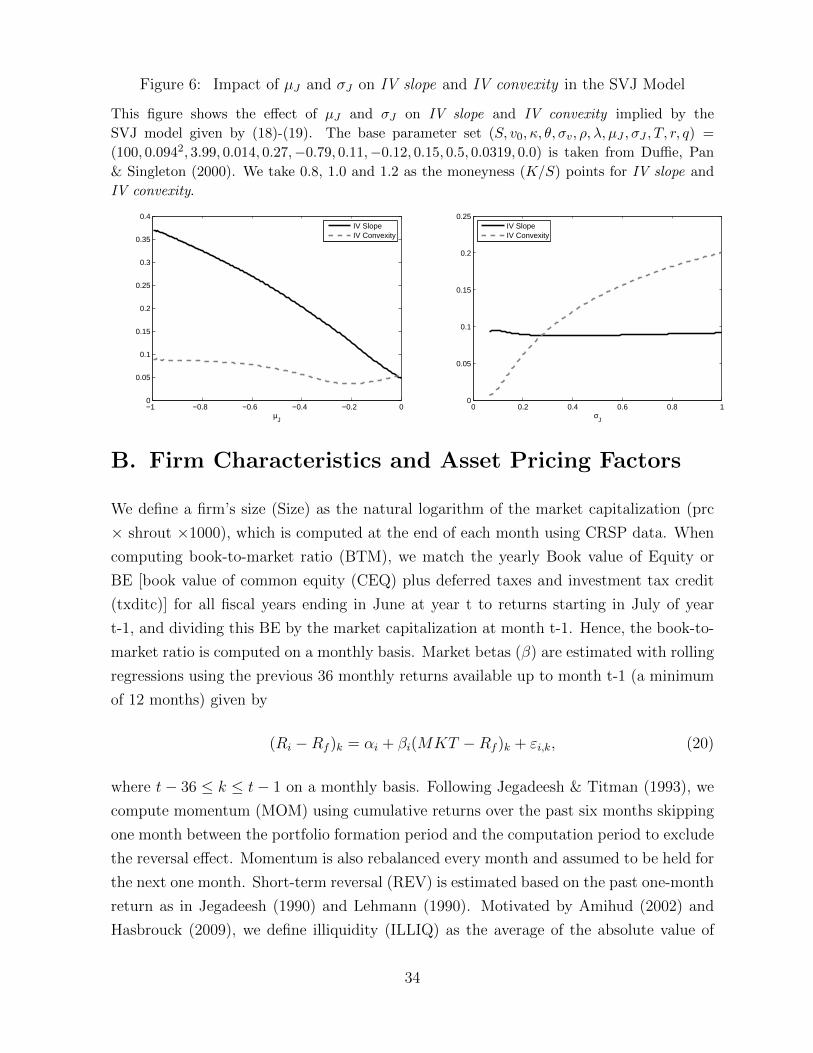
Figure 6: Impact of µJ and σJ on IV slope and IV convexity in the SVJ Model

This figure shows the effect of µJ and σJ on IV slope and IV convexity implied by the

SVJ model given by (18)-(19). The base parameter set (S, v0, κ, θ, σv, ρ, λ, µJ , σJ , T, r, q) =

(100, 0.0942, 3.99, 0.014, 0.27,−0.79, 0.11,−0.12, 0.15, 0.5, 0.0319, 0.0) is taken from Duffie, Pan

& Singleton (2000). We take 0.8, 1.0 and 1.2 as the moneyness (K/S) points for IV slope and

IV convexity.

−1 −0.8 −0.6 −0.4 −0.2 00

0.05

0.1

0.15

0.2

0.25

0.3

0.35

0.4

µJ


0 0.2 0.4 0.6 0.8 10

0.05

0.1

0.15

0.2

0.25

σJ


B. Firm Characteristics and Asset Pricing Factors

We define a firm’s size (Size) as the natural logarithm of the market capitalization (prc

× shrout ×1000), which is computed at the end of each month using CRSP data. When

computing book-to-market ratio (BTM), we match the yearly Book value of Equity or

BE [book value of common equity (CEQ) plus deferred taxes and investment tax credit

(txditc)] for all fiscal years ending in June at year t to returns starting in July of year

t-1, and dividing this BE by the market capitalization at month t-1. Hence, the book-to-

market ratio is computed on a monthly basis. Market betas (β) are estimated with rolling

regressions using the previous 36 monthly returns available up to month t-1 (a minimum

of 12 months) given by

(Ri −Rf )k = αi + βi(MKT −Rf )k + εi,k, (20)

where t− 36 ≤ k ≤ t− 1 on a monthly basis. Following Jegadeesh & Titman (1993), we

compute momentum (MOM) using cumulative returns over the past six months skipping

one month between the portfolio formation period and the computation period to exclude

the reversal effect. Momentum is also rebalanced every month and assumed to be held for

the next one month. Short-term reversal (REV) is estimated based on the past one-month

return as in Jegadeesh (1990) and Lehmann (1990). Motivated by Amihud (2002) and

Hasbrouck (2009), we define illiquidity (ILLIQ) as the average of the absolute value of

34

the stock return divided by the trading volume of the stock in thousand USD using the

past one-year’s daily data up to month t.

Following Harvey & Siddique (2000), we regress daily excess returns of individual

stocks on the daily market excess return and the daily squared market excess return using

a moving-window approach with an one-year window size. Specifically, we re-estimate the

regression model at each month-end, where the regression specification is given by

(Ri −Rf )k = αi + β1,i(MKT −Rf )k + β2,i(MKT −Rf )2k + εi,k, (21)

where t − 365 ≤ k ≤ t − 1 on a daily basis. Subsequently, the co-skewness (Coskew) is

defined as the coefficient of the squared market excess return. We require at least 225

trading days in a year to reduce the impact of infrequent trading.

We compute idiosyncratic volatility of stock returns according to Ang et al. (2006).

The daily excess returns of individual stocks over the last 30 days are regressed on daily

Fama-French three factors and momentum factors at the end of each month, where the

regression specification is given by

(Ri −Rf )k = αi + β1i(MKT −Rf )k + β2iSMBk + β3iHMLk + β4iWMLk + εk, (22)

where t − 30 ≤ k ≤ t − 1 on a daily basis. Idiosyncratic volatility is computed as the

standard deviation of the regression residuals. To reduce the impact of infrequent trading

on idiosyncratic volatility estimates, a minimum of 15 trading days in a month for which

CRSP reports both a daily return and non-zero trading volume is required.

We estimate systematic volatility using the method suggested by Duan & Wei (2009)

as v2sys = β2v2

M/v2 at the end of each month. Motivated by Dennis, Mayhew & Stivers

(2006), we compute idiosyncratic implied variance as v2idio = v2 − β2v2

M on a monthly

basis, where vM is the implied volatility of the S&P500 index option.

35

Tab

le1:

Des

crip

tive

Sta

tist

ics:

Opti

on-i

mplied

Vol

atilit

ies

Pan

elA

rep

orts

the

sum

mar

yst

atis

tics

ofth

efi

tted

imp

lied

vola

tili

ties

an

dfi

xed

del

tas

of

the

ind

ivid

ual

equ

ity

op

tion

sw

ith

on

em

onth

(30

day

s)to

exp

irat

ion

atth

een

dof

mon

thob

tain

edfr

om

Op

tion

Met

rics

.D

Sm

easu

res

the

deg

ree

of

acc

ura

cyin

the

fitt

ing

pro

cess

at

each

poin

t

and

com

pu

ted

by

the

wei

ghte

dav

erag

est

and

ard

dev

iati

on

s.P

an

elB

rep

ort

sth

esa

mp

led

istr

ibu

tion

of

un

iqu

efi

rms

by

year

an

din

du

stry

.E

ach

firm

isas

sign

edin

toon

eof

the

Fam

a-F

ren

ch12

ind

ust

ries

(FF

1-1

2)

class

ifica

tion

base

don

its

SIC

cod

e.T

he

sam

ple

per

iod

cove

rsJan

2000

toD

ec2013.

Pan

elA

.S

um

mar

yst

ati

stic

sof

the

fitt

edim

pli

edvo

lati

liti

esC

all

Op

tion

s∆

2025

3035

40

45

50

55

60

65

70

75

80

Mea

n0.

4942

0.48

170.

4739

0.4

696

0.4

677

0.4

676

0.4

694

0.4

730

0.4

779

0.4

841

0.4

917

0.5

019

0.5

157

std

ev0.

2774

0.27

640.

2755

0.2

746

0.2

735

0.2

724

0.2

722

0.2

732

0.2

744

0.2

763

0.2

783

0.2

808

0.2

840

DS

0.05

020.

0397

0.03

060.0

244

0.0

208

0.0

190

0.0

182

0.0

181

0.0

190

0.0

213

0.0

258

0.0

334

0.0

436

Pu

tO

pti

on

s∆

-80

-75

-70

-65

-60

-55

-50

-45

-40

-35

-30

-25

-20

Mea

n0.

4958

0.48

550.

4788

0.4

755

0.4

745

0.4

755

0.4

784

0.4

831

0.4

893

0.4

970

0.5

067

0.5

199

0.5

381

std

ev0.

2976

0.29

190.

2876

0.2

846

0.2

821

0.2

803

0.2

796

0.2

797

0.2

803

0.2

813

0.2

823

0.2

836

0.2

844

DS

0.04

520.

0369

0.02

890.0

231

0.0

197

0.0

181

0.0

178

0.0

183

0.0

198

0.0

228

0.0

285

0.0

382

0.0

514

Pan

elB

.S

am

ple

dis

trib

uti

on

by

year

and

ind

ust

ryY

ear

FF

1F

F2

FF

3F

F4

FF

5F

F6

FF

7F

F8

FF

9F

F10

FF

11

FF

12

Tota

l20

0012

159

214

94

56

700

165

81

263

229

332

586

2900

2001

8649

167

90

50

641

145

71

219

233

290

518

2559

2002

9145

170

88

58

539

94

73

235

246

333

493

2465

2003

9047

165

82

55

476

77

73

235

233

349

479

2361

2004

8949

178

100

53

515

94

79

248

271

372

522

2570

2005

9350

200

122

56

521

95

82

258

281

466

558

2782

2006

102

5423

1138

68

529

97

87

279

298

597

620

3100

2007

104

6324

8156

74

545

105

96

287

303

734

704

3419

2008

113

6324

6157

75

517

101

105

276

278

823

703

3457

2009

110

5623

2154

70

460

87

110

283

269

794

705

3330

2010

120

5623

7168

70

479

88

113

285

282

823

795

3516

2011

126

5825

4190

76

521

90

115

294

293

903

913

3833

2012

123

5625

1198

73

493

84

116

297

292

934

978

3895

2013

131

6325

2203

75

493

91

115

295

287

1069

1085

4159

36

Table 2: Descriptive Statistics: Shape of Implied Volatility Curves and FirmCharacteristics

This table reports the descriptive statistics of other variables used in the analysis. Panel A reports the descriptive statistics

of option-implied volatility, slope and convexity of implied volatility curves with one month (30 days) to expiration at the

end of each month. IVput(∆) and IVcall(∆) refer to the fitted put and call option-implied volatilities with one month

(30 days) to expiration, where ∆ is the options’ delta. IV level is defined as IV level = 0.5 × [IVput(−0.5) + IVcall(0.5)].

IV slope is computed by IV slope = IVput(−0.2) − IVput(−0.8). We adopt the definitions of IV spread and IV smirk

proposed by Yan (2011) and Xing et al. (2010), respectively. The convexity of option-implied volatility curve is calculated

by IV convexity = IVput(−0.2) + IVput(−0.8) − 2 × IVcall(0.5). Using daily options implied convexity of equity options

and S&P500 index option, we conduct time-series regressions per month to decompose option-implied convexity into

the systematic and idiosyncratic components given by IV convexityi,k = αi + βi × IV convexityS&P500,k + εi,k, where

t − 30 ≤ k ≤ t − 1 on a daily basis. The fitted values and residual terms are the systematic components (Convexitysys)

of options implied convexity and the idiosyncratic components (Convexityidio) of options implied convexity, respectively.

We select the observations at the end of each month. Panel B shows the descriptive statistics for each firm characteristics

(Size, BTM, Beta, MOM, REV, ILLIQ, Coskew). Size (ln mv) is computed at the end of each month and we define size

as natural logarithm of the market capitalization. When computing book-to-market ratio(BTM), we match the yearly BE

(book value of common equity (CEQ) plus deferred taxes and investment tax credit (txditc)) for all fiscal years ending

at year t-1 to returns starting in July of year t and this BE is divided by market capitalization at month t-1. Beta () is

estimated from time-series regressions of raw stock excess returns on the Rm-Rf by month-by-month rolling over past

three year (36 months) returns (a minimum of 12 months). Momentum (MOM) is computed based on past cumulative

returns over the past six months skipping one month between the portfolio formation period and the computation period to

exclude the reversal effect following Jegadeesh and Titman (1993). Reversal (REV) is computed based on past one-month

return following Jegadeesh (1990) and Lehmann (1990). Illiquidity (ILLIQ) is the average of the absolute value of stock

return divided by the trading volume of the stock in thousand USD calculated using the past one-year’s daily data up to

month t following Amihud (2002) and Hasbrouck(2009). Following Harvey and Siddique (2000), daily excess returns of

individual stocks are regressed on the daily market excess return and the daily squared market excess return using the

last one year data month by month given by (Ri − Rf )k = αi + β1,i(MKT − Rf )k + β2,i(MKT − Rf )2k + εi,k, where

t− 365 ≤ k ≤ t− 1 on a daily basis. The co-skewness of a stock is the coefficient of the squared market excess return. To

reduce the impact of infrequent trading on co-skewness estimates, we require a minimum of 255 trading days per month.

Panel A. The shape of option-implied volatility curveImplied Volatility Slope of Implied Volatility Curve Convexity of Implied Volatiltiy Curve

IV level IV slope IV spread IV smirk IV convexity IV convexitysys IV convexity idio

Mean 0.4739 0.0423 0.0090 0.0687 0.0952 0.0933 0.0019Stdev 0.2689 0.1614 0.1235 0.1413 0.2774 0.1703 0.2235

Median 0.4088 0.0422 0.0045 0.0516 0.0590 0.0655 -0.0053Observation 471112 471112 471112 471112 471112 471112 471112

Panel B. Variables of firm characteristicsSize BTM beta (β) MOM REV ILLIQ (×106) Coskew

Mean 19.4607 0.9186 1.1720 0.0966 0.0187 0.7808 -1.3516Median 19.3757 0.5472 0.9808 0.0461 0.0080 0.0183 -0.5745Stdev 2.1054 2.3613 1.1860 0.4515 0.1701 5.2832 15.2483

37

Table 3: Average returns sorted by option-implied volatility variables

This table reports the descriptive statistics of the average quintile portfolio returns (per month) sorted

by alternative measures of IV convexity. At the end of each month, all firms are assigned to one of five

portfolio groups based on alternative options implied convexity assuming that stocks are held for the next

one-month-period. This process is repeated in every month. Monthly stock returns are obtained from

the Center for Research in Security Prices (CRSP) with stocks traded on the NYSE (exchcd=1), Amex

(exchcd=2), and NASDAQ (exchcd=3). We use only common shares (shrcd in 10, 11). Stocks with a

price less than three dollars are excluded from the sample. “Q1-Q5” denotes an arbitrage portfolio that

buys a low option-implied convexity portfolio (Q1) and sells a high option-implied convexity portfolio

(Q5). The sample period covers Jan 2000 to Dec 2013. Value-weighted portfolio returns are weighted by

the lag of market capitalization of the underlying stocks. Numbers in parentheses indicate t-statistics.

Panel A. Equal-weighted and Value-weighted portfolio returns sorted by IV convexity

Quintile Avg # of firms Mean Stdev EW Return VW Return

Q1 (Low IV convexity) 432 -0.1364 0.2822 0.0208 0.0136Q2 423 0.0156 0.0317 0.0124 0.0061Q3 415 0.0637 0.0394 0.0098 0.0051Q4 404 0.1333 0.0672 0.009 0.0025

Q5 (High IV convexity) 389 0.398 0.3539 0.0074 0.0023

Q1-Q50.0134 0.0113(7.87) (5.08)

Panel B. Equal-weighted and Value-weighted portfolio returns sorted by IV spread


Q1 (Low IV spread) 425 -0.0834 0.1491 0.0145 0.0109Q2 434 -0.0094 0.0131 0.0102 0.0067Q3 425 0.004 0.0109 0.0081 0.0044Q4 396 0.0189 0.0173 0.0066 0.004

Q5 (High IV spread) 384 0.1096 0.1844 0.0013 -0.0004

Q1-Q50.0131 0.0113(7.31) (3.91)

Panel C. Equal-weighted and Value-weighted portfolio returns sorted by IV smirk


Q1 (Low IV smirk) 418 -0.0519 0.1462 0.0136 0.0112Q2 422 0.0292 0.0176 0.0099 0.0066Q3 417 0.0527 0.0202 0.0073 0.0035Q4 410 0.0845 0.0286 0.0066 0.0033

Q5 (High IV smirk) 396 0.2182 0.1863 0.0034 0.0019

Q1-Q50.0102 0.0094(5.05) (3.64)

38

Tab

le4:

Alt

ernat

ive

Mea

sure

sof

IVco

nve

xity

Th

ista

ble

rep

ort

sth

ed

escr

ipti

ve

stati

stic

sof

the

aver

age

qu

inti

lep

ort

folio

retu

rns

(per

month

)so

rted

by

alt

ern

ati

ve

mea

sure

sofIV

convexity

.IVput(∆

)an

dIVcall

(∆)

refe

rto

the

fitt

edp

ut

an

dca

llop

tion

-im

plied

vola

tiliti

esw

ith

on

em

onth

(30

days)

toex

pir

ati

on

,w

her

e∆

isth

eop

tion

s’del

ta.

At

the

end

of

each

month

,all

firm

sare

ass

ign

edto

on

e

of

five

port

folio

gro

up

sb

ase

don

alt

ern

ati

ve

op

tion

sim

plied

convex

ity

ass

um

ing

that

stock

sare

hel

dfo

rth

en

ext

on

e-m

onth

-per

iod

.T

his

pro

cess

isre

pea

ted

inev

ery

month

.

Month

lyst

ock

retu

rns

are

ob

tain

edfr

om

the

Cen

ter

for

Res

earc

hin

Sec

uri

tyP

rice

s(C

RS

P)

wit

hst

ock

str

ad

edon

the

NY

SE

(exch

cd=

1),

Am

ex(e

xch

cd=

2),

an

dN

AS

DA

Q

(exch

cd=

3).

We

use

on

lyco

mm

on

share

s(s

hrc

din

10,

11).

Sto

cks

wit

ha

pri

cele

ssth

an

thre

ed

ollars

are

excl

ud

edfr

om

the

sam

ple

.“Q

1-Q

5”

den

ote

san

arb

itra

ge

port

folio

that

bu

ys

alo

wop

tion

-im

plied

convex

ity

port

folio

(Q1)

an

dse

lls

ah

igh

op

tion

-im

plied

convex

ity

port

folio

(Q5).

Th

esa

mp

lep

erio

dco

ver

sJan

2000

toD

ec2013.

Pan

elA

rep

ort

s

des

crip

tive

stati

stic

sof

the

equal-

wei

ghte

dan

dvalu

e-w

eighte

daver

age

port

folio

retu

rns

(per

month

)so

rted

by

alt

ern

ati

veIV

convexity

mea

sure

sby

vary

ing

ITM

an

dO

TM

poin

ts,

defi

ned

as

p∆

1-c

50-p

∆2=IVput

(−∆

1)+IVput

(−∆

1)-

2×IVcall

(0.5

),w

her

e0.2

≤∆

1≤

0.4

5an

d0.5

5≤

∆2≤

0.8

.V

alu

e-w

eighte

dp

ort

folio

retu

rns

are

wei

ghte

dby

the

lag

of

mark

etca

pit

aliza

tion

of

the

un

der

lyin

gst

ock

s.In

Pan

elB

,th

ed

efin

itio

ns

ofIVconvexity(I

I)-IVconvexity(V

I)

are

giv

enby

(9)-

(13).

Nu

mb

ers

inp

are

nth

eses

ind

icate

t-st

ati

stic

s.

Pan

elA

.A

lter

nat

ive

mea

sure

sof

IVconvexity

by

vary

ing

ITM

and

OT

Mp

oints

p25

-c50

-p75

p30

-c50

-p70

p35

-c50

-p65

p40-c

50-p

60

p45-c

50-p

55

Quin

tile

Mea

nE

WR

etV

WR

etM

ean

EW

Ret

VW

Ret

Mea

nE

WR

etV

WR

etM

ean

EW

Ret

VW

Ret

Mea

nE

WR

etV

WR

etQ

1(L

ow)

-0.1

304

0.02

020.

0136

-0.1

364

0.0

199

0.01

06-0

.138

50.

0199

0.01

09-0

.1388

0.0

198

0.0

106

-0.1

395

0.0

204

0.0

116

Q2

0.00

100.

0120

0.00

58-0

.007

90.0

123

0.00

64-0

.013

00.

0124

0.00

61-0

.0155

0.0

124

0.0

063

-0.0

163

0.0

122

0.0

069

Q3

0.04

210.

0095

0.00

520.

0292

0.0

096

0.00

490.

0206

0.00

950.

0056

0.01

470.0

096

0.0

057

0.0

110

0.0

090

0.0

052

Q4

0.09

770.

0093

0.00

230.

0755

0.0

089

0.00

310.

0604

0.00

850.

0034

0.04

980.0

090

0.0

032

0.0

428

0.0

088

0.0

034

Q5

(Hig

h)

0.31

200.

0080

0.00

290.

2644

0.0

084

0.00

350.

2313

0.00

880.

0019

0.20

920.0

083

0.0

008

0.1

967

0.0

086

0.0

012

Q1-

Q5

0.01

220.

0106

0.0

115

0.00

710.

0111

0.00

900.0

115

0.0

098

0.0

118

0.0

104

(7.7

4)(4

.85)

(7.3

2)(3

.36)

(7.1

1)(3

.89)

(7.0

3)

(4.0

7)

(6.7

9)

(3.8

7)

Pan

elB

.A

lter

nat

ive

mea

sure

sof

IVconvexity

bet

wee

nca

lls

and

puts

IVconvexity(I

I)

IVconvexity(I

II)

IVconvexity(I

V)

IVconvexity(V

)IVconvexity(V

I)

Quin

tile

Mea

nStd

evA

vg

Ret

Mea

nStd

evA

vg

Ret

Mea

nStd

evA

vg

Ret

Mea

nStd

evA

vg

Ret

Mea

nStd

evA

vg

Ret

Q1

(Low

)-0

.056

00.

1615

0.00

95-0

.056

20.1

588

0.01

54-0

.040

70.

1191

0.01

90-0

.0571

0.1

627

0.0

177

-0.0

714

0.2

098

0.0

203

Q2

0.01

620.

0131

0.00

920.

0139

0.0

138

0.01

250.

0227

0.01

340.

0110

0.01

660.0

130

0.0

140

0.0

240

0.0

158

0.0

104

Q3

0.04

710.

0214

0.00

820.

0434

0.0

229

0.00

930.

0501

0.02

000.

0098

0.04

700.0

213

0.0

095

0.0

570

0.0

217

0.0

095

Q4

0.09

570.

0414

0.00

810.

0904

0.0

416

0.00

970.

0923

0.03

500.

0096

0.09

550.0

413

0.0

099

0.1

139

0.0

439

0.0

090

Q5

(Hig

h)

0.27

500.

2040

0.00

570.

2533

0.1

893

0.01

280.

2350

0.15

660.

0103

0.27

470.2

034

0.0

086

0.3

376

0.2

663

0.0

103

Q1-

Q5

0.00

380.0

026

0.008

70.0

091

0.0

100

(2.4

9)(1

.76)

(5.1

0)

(6.0

9)

(5.1

4)

39

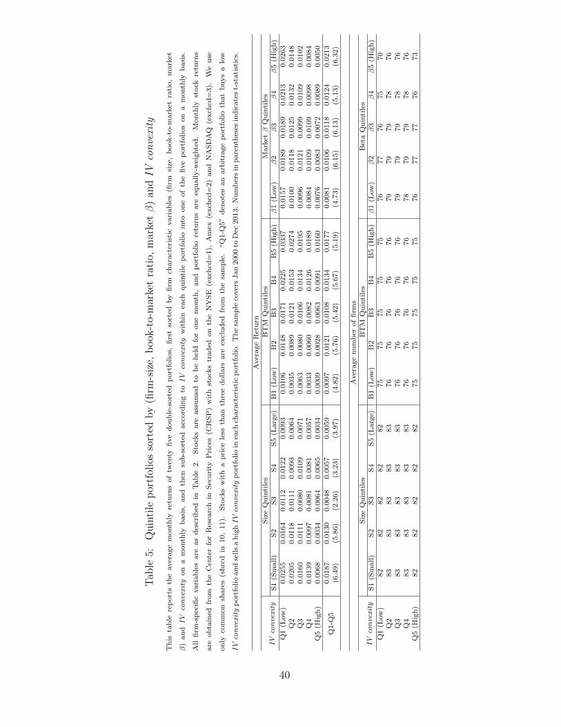
Tab

le5:

Quin

tile

por

tfol

ios

sort

edby

(firm

-siz

e,b

ook

-to-

mar

ket

rati

o,m

arke

tβ

)an

dIV

con

vexi

ty

Th

ista

ble

rep

ort

sth

eaver

age

month

lyre

turn

sof

twen

tyfi

ve

dou

ble

-sort

edp

ort

folios,

firs

tso

rted

by

firm

chara

cter

isti

cvari

ab

les

(firm

size

,b

ook-t

o-m

ark

etra

tio,

mark

et

β)

an

dIV

convexity

on

am

onth

lyb

asi

s,an

dth

ensu

b-s

ort

edacc

ord

ing

toIV

convexity

wit

hin

each

qu

inti

lep

ort

folio

into

on

eof

the

five

port

foli

os

on

am

onth

lyb

asi

s.

All

firm

-sp

ecifi

cvari

ab

les

are

as

des

crib

edin

Tab

le2.

Sto

cks

are

ass

um

edto

be

hel

dfo

ron

em

onth

,an

dp

ort

folio

retu

rns

are

equ

ally-w

eighte

d.

Month

lyst

ock

retu

rns

are

ob

tain

edfr

om

the

Cen

ter

for

Res

earc

hin

Sec

uri

tyP

rice

s(C

RS

P)

wit

hst

ock

str

ad

edon

the

NY

SE

(exch

cd=

1),

Am

ex(e

xch

cd=

2)

an

dN

AS

DA

Q(e

xch

cd=

3).

We

use

on

lyco

mm

on

share

s(s

hrc

din

10,

11).

Sto

cks

wit

ha

pri

cele

ssth

an

thre

ed

ollars

are

excl

ud

edfr

om

the

sam

ple

.“Q

1-Q

5”

den

ote

san

arb

itra

ge

port

folio

that

bu

ys

alo

w

IVconvexity

port

folio

an

dse

lls

ah

ighIV

convexity

port

folio

inea

chch

ara

cter

isti

cp

ort

folio.

Th

esa

mp

leco

ver

sJan

2000

toD

ec2013.

Nu

mb

ers

inp

are

nth

eses

ind

icate

st-

stati

stic

s.

Aver

age

Ret

urn

IVconvexity

Siz

eQ

uin

tile

sB

TM

Qu

inti

les

Mark

etβ

Qu

inti

les

S1

(Sm

all)

S2

S3

S4

S5

(Larg

e)B

1(L

ow

)B

2B

3B

4B

5(H

igh

)β

1(L

ow

)β

2β

3β

4β

5(H

igh

)Q

1(L

ow

)0.0

255

0.0

164

0.0

112

0.0

122

0.0

093

0.0

106

0.0

148

0.0

171

0.0

225

0.0

337

0.0

157

0.0

189

0.0

189

0.0

213

0.0

263

Q2

0.0

205

0.0

118

0.0

111

0.0

093

0.0

064

0.0

035

0.0

089

0.0

121

0.0

153

0.0

274

0.0

100

0.0

118

0.0

125

0.0

132

0.0

148

Q3

0.0

160

0.0

111

0.0

080

0.0

109

0.0

071

0.0

063

0.0

080

0.0

106

0.0

134

0.0

195

0.0

096

0.0

121

0.0

099

0.0

109

0.0

102

Q4

0.0

139

0.0

097

0.0

081

0.0

081

0.0

057

0.0

033

0.0

060

0.0

082

0.0

126

0.0

189

0.0

084

0.0

109

0.0

109

0.0

098

0.0

084

Q5

(Hig

h)

0.0

068

0.0

034

0.0

064

0.0

065

0.0

034

0.0

009

0.0

028

0.0

063

0.0

091

0.0

160

0.0

076

0.0

083

0.0

072

0.0

089

0.0

050

Q1-Q

50.0

187

0.0

130

0.0

048

0.0

057

0.0

059

0.0

097

0.0

121

0.0

108

0.0

134

0.0

177

0.0

081

0.0

106

0.0

118

0.0

124

0.0

213

(6.4

9)

(5.8

6)

(2.2

6)

(3.2

3)

(3.9

7)

(4.8

2)

(5.7

6)

(5.4

2)

(5.6

7)

(5.1

9)

(4.7

3)

(6.1

5)

(6.1

3)

(5.1

3)

(6.3

2)

Aver

age

nu

mb

erof

firm

s

IVconvexity

Siz

eQ

uin

tile

sB

TM

Qu

inti

les

Bet

aQ

uin

tile

sS

1(S

mall)

S2

S3

S4

S5

(Larg

e)B

1(L

ow

)B

2B

3B

4B

5(H

igh

)β

1(L

ow

)β

2β

3β

4β

5(H

igh

)Q

1(L

ow

)82

82

82

82

82

75

75

75

75

75

76

77

76

75

70

Q2

83

83

83

83

83

76

76

76

76

76

79

79

79

78

76

Q3

83

83

83

83

83

76

76

76

76

76

79

79

79

78

76

Q4

83

83

83

83

83

76

76

76

76

76

78

79

79

78

76

Q5

(Hig

h)

82

82

82

82

82

75

75

75

75

75

76

77

77

76

73

40

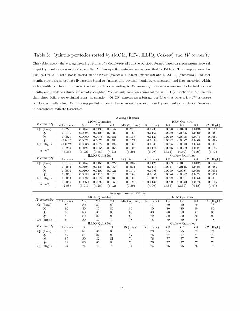
Table 6: Quintile portfolios sorted by (MOM, REV, ILLIQ, Coskew) and IV convexity

This table reports the average monthly returns of a double-sorted quintile portfolio formed based on (momentum, reversal,

illiquidity, co-skewness) and IV convexity. All firm-specific variables are as described in Table 2. The sample covers Jan

2000 to Dec 2013 with stocks traded on the NYSE (exchcd=1), Amex (exchcd=2) and NASDAQ (exchcd=3). For each

month, stocks are sorted into five groups based on (momentum, reversal, liquidity, co-skewness) and then subsorted within

each quintile portfolio into one of the five portfolios according to IV convexity. Stocks are assumed to be held for one

month, and portfolio returns are equally-weighted. We use only common shares (shrcd in 10, 11). Stocks with a price less

than three dollars are excluded from the sample. “Q1-Q5” denotes an arbitrage portfolio that buys a low IV convexity

portfolio and sells a high IV convexity portfolio in each of momentum, reversal, illiquidity, and coskew portfolios. Numbers

in parentheses indicate t-statistics.

Average Return

IV convexityMOM Quintiles REV Quintiles

M1 (Loser) M2 M3 M4 M5 (Winner) R1 (Low) R2 R3 R4 R5 (High)Q1 (Low) 0.0225 0.0157 0.0130 0.0147 0.0273 0.0237 0.0170 0.0160 0.0136 0.0134

Q2 0.0107 0.0094 0.0103 0.0100 0.0185 0.0160 0.0132 0.0096 0.0092 0.0083Q3 0.0025 0.0060 0.0078 0.0087 0.0183 0.0123 0.0119 0.0098 0.0075 0.0065Q4 -0.0012 0.0071 0.0070 0.0086 0.0177 0.0084 0.0092 0.0087 0.0066 0.0068

Q5 (High) -0.0029 0.0036 0.0072 0.0082 0.0166 0.0061 0.0095 0.0070 0.0055 0.0013

Q1-Q50.0254 0.0121 0.0058 0.0066 0.0108 0.0176 0.0076 0.0089 0.0081 0.0122(8.36) (5.92) (3.76) (4.51) (5.39) (6.99) (3.64) (4.69) (4.49) (5.73)

IV convexityILLIQ Quintiles Coskew Quintiles

I1 (Low) I2 I3 I4 I5 (High) C1 (Low) C2 C3 C4 C5 (High)Q1 (Low) 0.0108 0.0157 0.0165 0.0222 0.0302 0.0128 0.0169 0.0131 0.0132 0.0140

Q2 0.0081 0.0104 0.0135 0.0158 0.0231 0.0115 0.0111 0.0116 0.0085 0.0082Q3 0.0064 0.0100 0.0101 0.0127 0.0174 0.0098 0.0099 0.0087 0.0098 0.0057Q4 0.0053 0.0083 0.0110 0.0116 0.0162 0.0056 0.0086 0.0092 0.0074 0.0037

Q5 (High) 0.0051 0.0097 0.0072 0.0069 0.0109 -0.0003 0.0079 0.0091 0.0056 0.0013

Q1-Q50.0057 0.0060 0.0093 0.0153 0.0193 0.0130 0.0090 0.0040 0.0076 0.0127(2.88) (3.01) (4.28) (6.12) (6.39) (4.60) (3.83) (2.39) (4.18) (5.07)

Average number of firms

IV convexityMOM Quintiles REV Quintiles

M1 (Loser) M2 M3 M4 M5 (Winner) R1 (Low) R2 R3 R4 R5 (High)Q1 (Low) 80 80 80 80 79 77 79 79 79 78

Q2 80 80 80 80 80 80 80 80 80 80Q3 80 80 80 80 80 80 80 80 81 80Q4 80 80 80 80 80 79 80 80 80 80

Q5 (High) 80 80 80 79 78 78 79 79 79 78

IV convexityILLIQ Quintiles Coskew Quintiles

I1 (Low) I2 I3 I4 I5 (High) C1 (Low) C2 C3 C4 C5 (High)Q1 (Low) 83 81 83 83 78 73 75 75 75 74

Q2 87 81 82 83 77 76 77 77 77 76Q3 85 80 82 81 74 76 77 77 77 76Q4 82 80 80 80 73 76 77 77 77 76

Q5 (High) 74 74 75 75 74 74 76 76 76 75

41

Tab

le7:

Quin

tile

por

tfol

ios

sort

edby

(IV

slop

e,IV

spre

ad,

IVsm

irk

)an

dIV

con

vexi

ty

Th

ista

ble

rep

ort

sth

eaver

age

month

lyre

turn

sof

ad

ou

ble

-sort

edqu

inti

lep

ort

folio

form

edb

ase

don

(IV

slope

,IV

spread,IV

smirk

)an

dIV

convexity

.P

ort

folios

are

sort

edin

five

gro

up

sat

the

end

of

each

month

base

don

(IV

slope

,IV

spread,IV

smirk

)fi

rst

an

dth

ensu

b-s

ort

edin

tofi

ve

gro

up

sb

ase

donIV

convexity

.O

pti

on

svola

tility

slop

esare

com

pu

ted

byIVslope

=IVput(−

0.2

)−IVput(−

0.8

),IVspread

=IVput(−

0.5

)−IVcall

(0.5

),an

dIV

smirk

isco

mp

ute

db

ase

don

the

met

hod

sugges

ted

by

Xin

get

al.

(2010),

resp

ecti

vel

y.S

tock

sare

hel

dfo

ron

em

onth

,an

dp

ort

folio

retu

rns

are

equ

al-

wei

ghte

d.

Month

lyst

ock

retu

rns

are

ob

tain

edfr

om

the

Cen

ter

for

Res

earc

hin

Sec

uri

tyP

rice

s

(CR

SP

)w

ith

stock

str

ad

edon

the

NY

SE

(exch

cd=

1),

Am

ex(e

xch

cd=

2)

an

dN

AS

DA

Q(e

xc

hcd

=3).

We

use

on

lyco

mm

on

share

s(s

hrc

din

10,

11).

Sto

cks

wit

ha

pri

cele

ss

than

thre

ed

ollars

are

excl

ud

edfr

om

the

sam

ple

.“Q

1-Q

5”

den

ote

san

arb

itra

ge

port

folio

that

bu

ys

alo

wIV

convexity

port

folio

an

dse

lls

ah

igh

IVconvexity

port

folio

in

each

(IV

slope

,IV

spread,IV

smirk

)p

ort

folio.

Th

esa

mp

lep

erio

dco

ver

sJan

2000

toD

ec2013.

Nu

mb

ers

inpare

nth

eses

ind

icate

t-st

ati

stic

s.

Aver

age

Ret

urn

IVconvexity

IVslope

Qu

inti

les

IVspread

Qu

inti

les

IVsm

irk

Qu

inti

les

S1(L

ow

)S

2S

3S

4S

5(H

igh

)S

1(L

ow

)S

2S

3S

4S

5(H

igh

)S

1(L

ow

)S

2S

3S

4S

5(H

igh

)Q

1(L

ow

)0.0

267

0.0

270

0.0

178

0.0

160

0.0

151

0.0

320

0.0

163

0.0

123

0.0

138

0.0

130

0.0

116

0.0

098

0.0

110

0.0

110

0.0

113

Q2

0.0

165

0.0

164

0.0

115

0.0

111

0.0

136

0.0

228

0.0

132

0.0

092

0.0

085

0.0

122

0.0

112

0.0

073

0.0

048

0.0

097

0.0

077

Q3

0.0

126

0.0

101

0.0

079

0.0

089

0.0

123

0.0

189

0.0

102

0.0

073

0.0

067

0.0

091

0.0

090

0.0

063

0.0

054

0.0

063

0.0

074

Q4

0.0

079

0.0

070

0.0

081

0.0

070

0.0

089

0.0

150

0.0

111

0.0

091

0.0

074

0.0

059

0.0

101

0.0

060

0.0

068

0.0

054

0.0

028

Q5

(Hig

h)

0.0

039

0.0

085

0.0

066

0.0

113

0.0

087

0.0

167

0.0

104

0.0

078

0.0

076

0.0

028

0.0

042

0.0

048

0.0

061

0.0

052

-0.0

004

Q1-Q

50.0

227

0.0

185

0.0

112

0.0

047

0.0

064

0.0

153

0.0

059

0.0

045

0.0

063

0.0

102

0.0

074

0.0

049

0.0

049

0.0

058

0.0

116

(6.8

4)

(6.3

0)

(4.5

9)

(2.1

4)

(2.5

2)

(5.2

1)

(3.2

2)

(2.6

1)

(3.1

7)

(3.7

7)

(3.2

7)

(2.1

8)

(2.2

1)

(1.9

3)

(3.9

7)

Aver

age

nu

mb

erof

firm

s

IVconvexity

IVsl

op

eQ

uin

tile

sIV

spre

ad

Qu

inti

les

IVsm

irk

Qu

inti

les

S1(L

ow

)S

2S

3S

4S

5(H

igh

)S

1(L

ow

)S

2S

3S

4S

5(H

igh

)S

1(L

ow

)S

2S

3S

4S

5(H

igh

)Q

1(L

ow

)82

85

86

88

86

85

88

85

82

80

46

47

48

49

48

Q2

80

82

86

87

86

87

85

83

77

75

47

47

47

47

46

Q3

79

83

86

86

84

85

87

85

78

76

46

47

46

46

43

Q4

77

81

83

84

80

86

89

87

79

76

45

45

44

44

42

Q5

(Hig

h)

77

79

80

80

77

82

86

85

79

77

42

43

41

41

38

42

Tab

le8:

Ave

rage

por

tfol

iore

turn

sso

rted

by

syst

emat

ican

did

iosy

ncr

atic

com

pon

ents

ofIV

con

vexi

ty

Pan

elA

rep

ort

the

des

crip

tive

stati

stic

sof

the

aver

age

port

foli

ore

turn

sso

rted

by

syst

emati

cco

mp

on

ents

(convexitysys)

an

did

iosy

ncr

ati

cco

mp

on

ents

(convexityid

io)

ofIV

convexity

.A

llfi

rm-s

pec

ific

vari

ab

les

are

as

des

crib

edin

Tab

le2.

At

the

end

of

each

month

,all

firm

sare

ass

ign

edin

toon

eof

five

port

folio

gro

up

sbase

don

IVconvexity

,

(convexitysys,convexityid

io)

an

dw

eass

um

est

ock

sare

hel

dfo

rth

en

ext

on

e-m

onth

-per

iod

.T

his

pro

cess

isre

pea

ted

inev

ery

month

.P

an

elB

rep

ort

sth

eaver

age

month

lyre

turn

s

of

ad

ou

ble

-sort

edqu

inti

lep

ort

folio

usi

ng

syst

emati

cco

mp

on

ents

ofIV

convexity

(convexitysys)

an

did

iosy

ncr

ati

cco

mp

on

ents

ofIV

convexity

(convexityid

io).

Port

folios

are

sort

edin

tofi

ve

gro

up

sat

the

end

of

each

month

base

don

(convexitysys,convexityid

io)

firs

t,an

dth

ensu

b-s

ort

edin

tofi

ve

gro

up

sb

ase

donIV

convexity

.S

tock

sare

hel

dfo

ron

e

month

,an

dp

ort

folio

retu

rns

are

equ

al-

wei

ghte

d.

Sto

cks

are

ass

um

edto

be

hel

dfo

ron

em

onth

,and

port

folio

retu

rns

are

equ

ally-w

eighte

d.

Month

lyst

ock

retu

rns

are

ob

tain

ed

from

the

Cen

ter

for

Res

earc

hin

Sec

uri

tyP

rice

s(C

RS

P)

wit

hst

ock

str

ad

edon

the

NY

SE

(exch

cd=

1),

Am

ex(e

xch

cd=

2)

an

dN

AS

DA

Q(e

xch

cd=

3).

We

use

on

lyco

mm

on

share

s(s

hrc

din

10,

11)

of

wh

ich

stock

pri

ceex

ceed

sth

ree

dollars

are

excl

ud

edfr

om

the

sam

ple

.“Q

1-Q

5”

den

ote

san

arb

itra

ge

port

folio

that

bu

ys

alo

wIV

convexity

port

folio

an

dse

lls

ah

ighIV

convexity

port

folio

inea

ch(convexitysys,convexityid

io)

port

folio.

Th

esa

mp

lep

erio

dco

ver

sJan

2000

toD

ec2013.

Nu

mb

ers

inp

are

nth

eses

ind

icate

t-st

ati

stic

s.

Pan

elA

.S

yst

emat

ican

did

iosy

ncr

atic

com

pon

ents

ofIV

convexity

and

aver

age

por

tfol

iore

turn

IVconvexity

convexitysys

convexityid

io

Avg

#of

firm

sM

ean

Std

evA

vg

Ret

Avg

#of

firm

sM

ean

Std

evA

vg

Ret

Q1

(Low

)423

-0.0

434

0.1

517

0.0

199

420

-0.2

113

0.2

402

0.0

174

Q2

426

0.0

373

0.0

199

0.0

111

419

-0.0

518

0.0

383

0.0

117

Q3

420

0.0

682

0.0

260

0.0

100

413

-0.0

039

0.0

330

0.0

116

Q4

410

0.1

145

0.0

425

0.0

094

408

0.0

470

0.0

483

0.0

101

Q5

(Hig

h)

385

0.2

773

0.2

113

0.0

089

403

0.2

379

0.2

781

0.0

087

Q1-Q

50.0

110

0.0

086

(6.5

6)

(5.7

2)

Pan

elB

.D

ou

ble

sort

edqu

inti

lep

ortf

olio

byconvexity sys

andconvexity idio

IVconvexity

Aver

age

Ret

urn

c sys1

c sys2

c sys3

c sys4

c sys5

c idio

1c i

dio

2c i

dio

3c i

dio

4c i

dio

5Q

1(L

ow

)0.0

319

0.0

158

0.0

156

0.0

143

0.0

155

0.0

152

0.0

145

0.0

130

0.0

111

0.0

049

Q2

0.0

224

0.0

122

0.0

091

0.0

091

0.0

095

0.0

129

0.0

107

0.0

105

0.0

081

0.0

044

Q3

0.0

188

0.0

090

0.0

079

0.0

101

0.0

094

0.0

115

0.0

093

0.0

079

0.0

075

0.0

059

Q4

0.0

131

0.0

102

0.0

088

0.0

077

0.0

070

0.0

101

0.0

064

0.0

095

0.0

068

0.0

007

Q5

(Hig

h)

0.0

140

0.0

086

0.0

090

0.0

059

0.0

029

0.0

049

0.0

065

0.0

079

0.0

057

-0.0

033

Q1-Q

50.0

179

0.0

072

0.0

066

0.0

084

0.0

126

0.0

102

0.0

080

0.0

051

0.0

053

0.0

082

(5.9

3)

(3.4

9)

(3.2

4)

(4.0

7)

(5.4

5)

(3.1

6)

(3.6

6)

(2.6

3)

(2.7

1)

(3.3

0)

IVconvexity

Aver

age

nu

mb

erof

firm

sc s

ys1

c sys2

c sys3

c sys4

c sys5

c idio

1c i

dio

2c i

dio

3c i

dio

4c i

dio

5Q

1(L

ow

)553

775

776

762

665

631

767

713

741

737

Q2

691

676

736

741

644

783

753

659

732

790

Q3

677

646

713

713

604

801

753

696

755

754

Q4

702

696

726

709

561

755

754

730

745

709

Q5

(Hig

h)

686

766

767

721

478

605

672

686

663

590

43

Tab

le9:

Shor

t-se

llin

gco

nst

rain

tsan

din

form

atio

nas

ym

met

ry

Th

ista

ble

rep

ort

sth

eaver

age

month

lyre

turn

sof

twen

tyfi

ve

dou

ble

-sort

edp

ort

folios,

firs

tso

rted

by

the

pre

vio

us

qu

art

erly

per

centa

ge

of

share

sou

tsta

nd

ing

hel

dby

inst

itu

tion

s

(fro

mth

eT

hom

son

Fin

an

cial

Inst

itu

tion

al

Hold

ings

(13F

)d

ata

base

),p

revio

us

qu

art

er’s

an

aly

stco

ver

age

(fro

mI/

B/E

/S

),p

revio

us

qu

art

er’s

an

aly

stfo

reca

std

isp

ersi

on

(fro

m

I/B

/E

/S

)an

dth

ensu

b-s

ort

edacc

ord

ing

toIV

convexity

wit

hin

each

qu

inti

lep

ort

folio

into

on

eof

the

five

port

folios

on

am

onth

lyb

asi

s.F

ollow

ing

Cam

pb

ell

etal.

(2008)

an

d

Nagel

(2005),

we

calc

ula

teth

esh

are

of

inst

itu

tion

al

ow

ner

ship

by

sum

min

gth

est

ock

hold

ings

of

all

rep

ort

ing

inst

itu

tion

sfo

rea

chst

ock

inea

chqu

art

er.

An

aly

stfo

reca

st

dis

per

sion

ism

easu

red

as

the

scale

dst

an

dard

dev

iati

on

of

I/B

/E

/S

an

aly

sts’

curr

ent

fisc

al

yea

rea

rnin

gs

per

share

fore

cast

sby

the

met

hod

inD

ieth

eret

al.

(2002).

Sto

cks

are

ass

um

edto

be

hel

dfo

ron

em

onth

,an

dp

ort

foli

ore

turn

sare

equ

ally-w

eighte

d.

Month

lyst

ock

retu

rns

are

ob

tain

edfr

om

the

Cen

ter

for

Res

earc

hin

Sec

uri

tyP

rice

s(C

RS

P)

wit

h

stock

str

ad

edon

the

NY

SE

(exch

cd=

1),

Am

ex(e

xch

cd=

2)

an

dN

AS

DA

Q(e

xch

cd=

3).

We

use

on

lyco

mm

on

share

s(s

hrc

din

10,

11)

of

wh

ich

pri

ceex

ceed

s.th

ree

dollars

.

Q1-Q

5d

enote

san

arb

itra

ge

port

folio

that

bu

ys

alo

wIV

convexity

port

folio

an

dse

lls

ah

ighIV

convexity

port

folio

inea

chch

ara

cter

isti

cp

ort

folio.

Th

esa

mp

leco

ver

sJan

2000

toD

ec2013.

Nu

mb

ers

inp

are

nth

eses

ind

icate

st-

stati

stic

s.

Aver

ave

Ret

urn

IVconvexity

F-1

3fi

lin

gs(

Inst

itu

tion

al

Hold

ings)

An

aly

stC

over

age

An

aly

stF

ore

cast

Dis

per

sion

F1(L

ow

)F

2F

3F

4F

5(H

igh

)A

C1(L

ow

)A

C2

AC

3A

C4

AC

5(H

igh

)A

D1(L

ow

)A

D2

AD

3A

D4

AD

5(H

igh

)Q

1(L

ow

)0.0

228

0.0

215

0.0

210

0.0

195

0.0

150

0.0

230

0.0

228

0.0

195

0.0

169

0.0

177

0.0

225

0.0

207

0.0

215

0.0

190

0.0

151

Q2

0.0

150

0.0

141

0.0

132

0.0

117

0.0

084

0.0

156

0.0

151

0.0

122

0.0

107

0.0

094

0.0

161

0.0

139

0.0

118

0.0

115

0.0

089

Q3

0.0

103

0.0

083

0.0

103

0.0

112

0.0

075

0.0

129

0.0

115

0.0

102

0.0

098

0.0

084

0.0

140

0.0

108

0.0

087

0.0

091

0.0

014

Q4

0.0

088

0.0

124

0.0

117

0.0

101

0.0

066

0.0

118

0.0

122

0.0

098

0.0

087

0.0

081

0.0

144

0.0

126

0.0

095

0.0

088

0.0

035

Q5

(Hig

h)

0.0

064

0.0

096

0.0

086

0.0

124

0.0

085

0.0

086

0.0

087

0.0

086

0.0

078

0.0

063

0.0

145

0.0

121

0.0

099

0.0

061

-0.0

011

Q1-Q

50.0

164

0.0

120

0.0

124

0.0

071

0.0

065

0.0

145

0.0

141

0.0

109

0.0

091

0.0

114

0.0

081

0.0

086

0.0

116

0.0

129

0.0

162

(5.1

8)

(4.4

4)

(5.7

8)

(3.3

8)

(3.3

4)

(4.9

3)

(5.0

2)

(4.3

6)

(4.6

0)

(5.2

1)

(3.7

6)

(4.4

6)

(4.8

7)

(5.3

4)

(5.4

6)

Aver

age

nu

mb

erof

firm

s

IVconvexity

F-1

3fi

lin

gs

(In

stit

uti

on

al

Hold

ings)

An

aly

stC

over

age

An

aly

stF

ore

cast

Dis

per

sion

F1(L

ow

)F

2F

3F

4F

5(H

igh

)A

C1(L

ow

)A

C2

AC

3A

C4

AC

5(H

igh

)A

D1(L

ow

)A

D2

AD

3A

D4

AD

5(H

igh

)Q

1(L

ow

)49

51

52

51

51

60

70

74

73

76

71

71

70

67

61

Q2

49

54

54

53

55

58

71

76

75

78

75

74

73

71

64

Q3

49

54

54

53

54

59

71

75

74

78

75

74

73

70

64

Q4

48

53

53

52

54

57

69

74

74

78

73

73

71

68

61

Q5

(Hig

h)

46

51

51

49

51

56

66

70

71

75

70

69

67

63

55

44

Tab

le10

:T

ime-

seri

esan

alysi

sof

CA

PM

and

Fam

a-F

rench

thre

ean

dfo

ur

fact

orm

odel

s

Th

ista

ble

pre

sents

the

coeffi

cien

tes

tim

ates

of

CA

PM

an

dF

am

a-F

ren

chth

ree

an

dfo

ur

fact

or

mod

els

for

month

lyex

cess

retu

rns

onIV

convexity

qu

inti

les

por

tfol

ios.

Fam

a-F

ren

chfa

ctor

s[R

M−R

f,

small

mark

etca

pit

ali

zati

on

min

us

big

(SM

B),

an

dh

igh

book-t

o-m

ark

etra

tio

min

us

low

(HM

L),

and

mom

entu

mfa

ctor

(UM

D)]

are

obta

ined

from

Ken

net

hF

ren

ch’s

web

site

.T

he

sam

ple

per

iod

cove

rsJan

2000

toD

ec2013

wit

hst

ock

str

ad

edon

the

NY

SE

(exch

cd=

1),

Am

ex(e

xch

cd=

2)an

dN

AS

DA

Q(e

xch

cd=

3).

Sto

cks

wit

ha

pri

cele

ssth

an

thre

ed

oll

ars

are

excl

ud

edfr

om

the

sam

ple

,an

d

New

ey&

Wes

t(1

987)

adju

sted

t-st

atis

tics

are

rep

ort

edin

squ

are

bra

cket

s.

Model

Facto

rsIV

convexity

convexitysys

convexityidio

Q1

Q2

Q3

Q4

Q5

Q1-Q

5Q1

Q2

Q3

Q4

Q5

Q1-Q

5Q1

Q2

Q3

Q4

Q5

Q1-Q

5

CAPM

Alp

ha

0.0146

0.0069

0.0042

0.0032

0.0014

0.0132

0.0138

0.0056

0.0043

0.0035

0.0031

0.0107

0.0113

0.0061

0.0061

0.0044

0.0026

0.0087

(5.60)

(4.75)

(2.88)

(2.04)

(0.66)

(7.72)

(5.51)

(3.96)

(2.83)

(2.05)

(1.53)

(6.39)

(4.70)

(3.92)

(4.41)

(2.88)

(1.20)

(5.62)

MKTRF

1.4472

1.2075

1.2505

1.3057

1.3830

0.0642

1.4207

1.2283

1.2811

1.3393

1.3338

0.0870

1.4086

1.2623

1.2307

1.2831

1.4110

-0.0024

(23.11)

(31.82)

(36.13)

(34.53)

(27.20)

(1.38)

(25.71)

(33.44)

(35.29)

(30.46)

(27.65)

(2.06)

(25.73)

(30.01)

(33.77)

(35.37)

(29.21)

(-0.06)

Adj.R

20.7920

0.8968

0.9065

0.9007

0.8500

0.0126

0.0126

0.9057

0.9003

0.8858

0.8494

0.0295

0.0295

0.8932

0.9128

0.9017

0.8442

¡0.0001

FF3

Alp

ha

0.0124

0.0048

0.0023

0.0011

-0.0010

0.0134

0.0118

0.0039

0.0024

0.0011

0.0004

0.0114

0.0087

0.0038

0.0042

0.0025

0.0005

0.0082

(5.87)

(4.52)

(2.34)

(1.03)

(-0.64)

(7.75)

(6.00)

(3.69)

(2.47)

(0.90)

(0.26)

(7.48)

(4.60)

(3.62)

(4.12)

(2.49)

(0.31)

(5.36)

MKTRF

1.3027

1.1149

1.1512

1.2026

1.2650

0.0377

1.2767

1.1361

1.1724

1.2278

1.2313

0.0454

1.2713

1.1624

1.1475

1.1776

1.2796

-0.0083

(23.58)

(37.48)

(44.49)

(40.90)

(28.50)

(0.85)

(28.30)

(38.33)

(46.30)

(34.29)

(29.01)

(1.38)

(25.92)

(36.13)

(38.38)

(43.02)

(29.43)

(-0.20)

SM

B0.6328

0.4493

0.4557

0.4824

0.5520

0.0808

0.6199

0.4238

0.4955

0.5324

0.5111

0.1088

0.6300

0.4786

0.4016

0.4772

0.5825

0.0475

(5.33)

(8.39)

(9.74)

(8.46)

(5.76)

(1.44)

(5.55)

(8.44)

(11.93)

(7.58)

(5.01)

(2.41)

(5.85)

(8.64)

(7.18)

(9.60)

(5.91)

(0.91)

HM

L0.0211

0.1346

0.0717

0.1006

0.1138

-0.0927

-0.0094

0.0685

0.0690

0.1377

0.1863

-0.1957

0.0995

0.1277

0.1146

0.0573

0.0386

0.0609

(0.23)

(2.71)

(1.70)

(2.44)

(1.67)

(-1.27)

(-0.12)

(1.42)

(1.73)

(2.51)

(2.70)

(-3.48)

(1.19)

(2.39)

(2.65)

(1.31)

(0.61)

(0.84)

Adj.R

20.8685

0.9541

0.9642

0.9585

0.9133

0.0491

0.0491

0.9572

0.9654

0.9508

0.9063

0.1781

0.1781

0.9527

0.9576

0.9625

0.9159

¡0.0001

FF4

Alp

ha

0.0132

0.0050

0.0024

0.0014

-0.0003

0.0136

0.0126

0.0040

0.0026

0.0015

0.0011

0.0115

0.0094

0.0042

0.0044

0.0028

0.0011

0.0083

(7.33)

(5.10)

(2.48)

(1.54)

(-0.29)

(7.61)

(7.55)

(3.94)

(2.90)

(1.48)

(0.90)

(7.32)

(5.85)

(4.63)

(4.58)

(2.93)

(0.88)

(5.32)

MKTRF

1.1125

1.0580

1.1264

1.1304

1.1112

0.0013

1.1050

1.1005

1.1200

1.1355

1.0804

0.0246

1.1044

1.0793

1.0974

1.1272

1.1380

-0.0336

(18.13)

(34.90)

(37.00)

(38.48)

(27.91)

(0.02)

(19.37)

(34.59)

(42.41)

(34.70)

(29.53)

(0.54)

(20.55)

(40.32)

(35.53)

(36.75)

(25.76)

(-0.69)

SM

B0.7588

0.4870

0.4722

0.5302

0.6539

0.1049

0.7336

0.4474

0.5302

0.5935

0.6110

0.1226

0.7406

0.5336

0.4348

0.5106

0.6763

0.0643

(7.28)

(11.09)

(9.97)

(11.01)

(8.59)

(1.51)

(7.50)

(9.27)

(13.78)

(10.08)

(7.54)

(2.09)

(7.64)

(12.92)

(8.60)

(11.41)

(8.01)

(1.04)

HM

L-0

.0143

0.1240

0.0671

0.0871

0.0852

-0.0995

-0.0413

0.0619

0.0592

0.1206

0.1582

-0.1995

0.0684

0.1122

0.1053

0.0480

0.0123

0.0561

(-0.22)

(3.02)

(1.64)

(2.52)

(1.86)

(-1.36)

(-0.68)

(1.35)

(1.78)

(3.06)

(3.89)

(-3.30)

(1.20)

(3.10)

(2.89)

(1.22)

(0.23)

(0.80)

UM

D-0

.3321

-0.0994

-0.0433

-0.1261

-0.2686

-0.0635

-0.2999

-0.0622

-0.0915

-0.1612

-0.2635

-0.0364

-0.2916

-0.1452

-0.0875

-0.0880

-0.2474

-0.0441

(-4.35)

(-4.37)

(-1.77)

(-7.22)

(-11.29)

(-0.97)

(-3.96)

(-2.40)

(-4.13)

(-7.41)

(-9.08)

(-0.61)

(-4.59)

(-5.23)

(-3.86)

(-4.63)

(-6.43)

(-0.84)

Adj.R

20.9232

0.9619

0.9654

0.9694

0.9553

0.0675

0.0675

0.9600

0.9713

0.9675

0.9497

0.1813

0.9324

0.9681

0.9635

0.9679

0.9499

0.0025

45

Table 11: Fama-MacBeth regressions

This table reports the averages of month-bymonth Fama & MacBeth (1973) cross-sectional regression coefficient estimates

for individual stock returns on IV convexity and control variables. The cross-section of expected stock returns is regressed

on control variables. Control variables include market β estimated by Fama & French (1992), size (ln mv), book-to-market

(btm), momentum (MOM), reversal (REV), illiquidity (ILLIQ), IV slope, idiosyncratic risk (idio risk), implied volatility

level (IV level), systematic volatility (v2sys), idiosyncratic implied variance (v2idio). All firm-specific variables are as

described in Table 2. Following Ang et al. (2006), we regress daily excess returns of individual stocks on the Fama-French

four factors daily in every month as (Ri − Rf )k = αi + β1i(MKT − Rf )k + β2iSMBk + β3iHMLk + β4iWMLk + εk,

where t − 30 ≤ k ≤ t − 1 on a daily basis. The idiosyncratic volatility of a stock (idio risk) is computed as the standard

deviation of the regression residuals. Systematic volatility is estimated by the method suggested by Duan & Wei (2009)

as v2sys = β2v2m/v2. Idiosyncratic implied variance is computed as v2idio = v2 − β2v2M , where vm is the implied volatility

of S&P500 index option, as suggested by Dennis et al. (2006). The daily factor data are downloaded from Kenneth R.

French’s website. To reduce the impact of infrequent trading on idiosyncratic volatility estimates, we require a minimum of

15 trading days in a month for which CRSP reports both a daily return and non-zero trading volume. The sample period

covers Jan 2000 to Dec 2013 with stocks traded on the NYSE (exchcd=1), Amex (exchcd=2) and NASDAQ (exchcd=3)

and stocks with a price less than three dollars are excluded from the sample. The adjusted t-statistics based on Newey

& West (1987) using lag of 3 are reported for the time-series average of coefficients. An intercept is included in each

specification but not reported in the table. Numbers in parentheses indicate t-statistics.

Variable MODEL 1 MODEL 2 MODEL 3 MODEL 4 MODEL 5 MODEL 6 MODEL 7 MODEL 8IV -0.015*** -0.017*** -0.015*** -0.016*** -0.015*** -0.017*** -0.015*** -0.017***

convexity (-6.60) (-6.19) (-6.70) (-6.38) (-6.61) (-6.17) (-6.59) (-6.17)IV -0.004 -0.004 -0.005 -0.005slope (-0.98) (-1.26) (-1.41) (-1.30)

Beta 0.001 0.001 0.000 0.000 0.000 0.000 0.001 0.001(0.33) (0.34) (0.20) (0.22) (0.25) (0.27) (0.41) (0.45)

Log(MV)-0.002** -0.002** -0.002*** -0.002*** -0.002*** -0.002*** -0.002*** -0.002***(-2.39) (-2.30) (-2.86) (-2.75) (-3.26) (-3.11) (-2.85) (-2.71)

Btm 0.004** 0.004** 0.004** 0.004** 0.003** 0.003** 0.004** 0.004**(2.14) (2.15) (2.24) (2.27) (2.15) (2.18) (2.18) (2.22)

MOM 0.001 0.001 0.001 0.001 0.001 0.001(0.15) (0.18) (0.28) (0.31) (0.21) (0.24)

REV-0.017*** -0.017*** -0.017*** -0.017*** -0.017*** -0.017***

(-3.47) (-3.45) (-3.48) (-3.46) (-3.43) (-3.42)

ILLIQ -0.007 -0.007 0.002 0.001 0.001 0.000(-0.37) (-0.36) (0.09) (0.07) (0.04) (0.02)

idio risk -0.110** -0.104*(-2.00) (-1.90)

IV -0.007 -0.007level (-1.05) (-1.01)

v2sys-0.002 -0.002(-1.52) (-1.58)

v2idio-0.008* -0.008*(-1.82) (-1.81)

Adj.R2 0.050 0.051 0.064 0.065 0.068 0.068 0.067 0.068

46

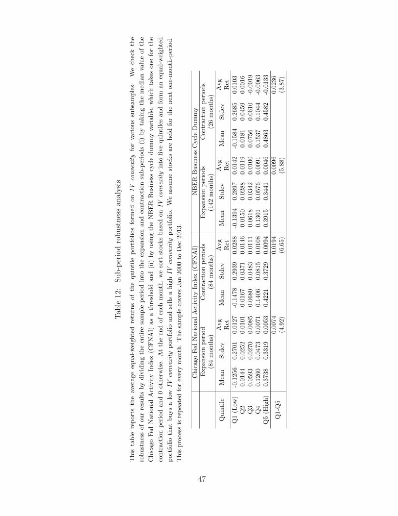
Tab

le12

:Sub-p

erio

dro

bust

nes

san

alysi

s

Th

ista

ble

rep

orts

the

aver

age

equ

al-w

eigh

ted

retu

rns

of

the

qu

inti

lep

ort

foli

os

form

edon

IVconvexity

for

vari

ou

ssu

bsa

mp

les.

We

chec

kth

e

rob

ust

nes

sof

our

resu

lts

by

div

idin

gth

een

tire

sam

ple

per

iod

into

the

exp

an

sion

an

dco

ntr

act

ion

sub

-per

iod

s(i

)by

takin

gth

em

edia

nva

lue

of

the

Ch

icag

oF

edN

atio

nal

Act

ivit

yIn

dex

(CF

NA

I)as

ath

resh

old

an

d(i

i)by

usi

ng

the

NB

ER

Bu

sin

ess

cycl

ed

um

my

vari

ab

le,

wh

ich

takes

on

efo

rth

e

contr

acti

onp

erio

dan

d0

oth

erw

ise.

At

the

end

of

each

month

,w

eso

rtst

ock

sbase

donIV

convexity

into

five

qu

inti

les

an

dfo

rman

equ

al-

wei

ghte

d

por

tfol

ioth

atb

uys

alo

wIV

convexity

por

tfol

ioan

dse

lls

ah

ighIV

convexity

port

foli

o.

We

ass

um

est

ock

sare

hel

dfo

rth

en

ext

on

e-m

onth

-per

iod

.

Th

isp

roce

ssis

rep

eate

dfo

rev

ery

mon

th.

The

sam

ple

cove

rsJan

2000

toD

ec2013.

Ch

icag

oF

edN

atio

nal

Act

ivit

yIn

dex

(CF

NA

I)N

BE

RB

usi

nes

sC

ycl

eD

um

my

Exp

ansi

onp

erio

dC

ontr

act

ion

per

iod

sE

xp

an

sion

per

iod

sC

ontr

act

ion

per

iods

(84

mon

ths)

(84

month

s)(1

42

month

s)(2

6m

onth

s)

Qu

inti

leM

ean

Std

evA

vg

Mea

nS

tdev

Avg

Mea

nS

tdev

Avg

Mea

nS

tdev

Avg

Ret

Ret

Ret

Ret

Q1

(Low

)-0

.125

60.

2701

0.0127

-0.1

478

0.2

939

0.0

288

-0.1

394

0.2

897

0.0

142

-0.1

584

0.2

685

0.0

103

Q2

0.01

440.

0252

0.0

101

0.0

167

0.0

371

0.0

146

0.0

150

0.0

288

0.0

119

0.0

181

0.0

459

0.0

016

Q3

0.05

930.

0270

0.0

085

0.0

680

0.0

483

0.0

111

0.0

618

0.0

342

0.0

100

0.0

756

0.0

610

-0.0

019

Q4

0.12

600.

0473

0.0

071

0.1

406

0.0

815

0.0

108

0.1

301

0.0

576

0.0

091

0.1

537

0.1

044

-0.0

063

Q5

(Hig

h)

0.37

380.

3319

0.0

053

0.4

221

0.3

729

0.0

094

0.3

915

0.3

441

0.0

046

0.4

863

0.4

582

-0.0

133

Q1-

Q5

0.0074

0.0

194

0.0

096

0.0

236

(4.9

2)

(6.6

5)

(5.8

8)

(3.8

7)

47

A Smiling Bear in the Equity Options Market and the Cross ... · A Smiling Bear in the Equity...

Documents

Transcript of A Smiling Bear in the Equity Options Market and the Cross ... · A Smiling Bear in the Equity...