A small macro econometric model of the US economy - SSB

Statistisk sentralbyråStatistics Norway

B Returadresse:Statistisk sentralbyråNO-2225 Kongsvinger

Documents

Documents

Statistics Norway

Oslo:PO Box 8131 DeptNO-0033 OsloTel.: + 47 21 09 00 00Fax: + 47 21 09 00 40

Kongsvinger:NO-2225 KongsvingerTel.: + 47 62 88 50 00Fax: + 47 62 88 50 30

E-mail: [email protected]: www.ssb.no

ISSN 0805-9411

Andreas Benedictow

A small macro econometric modelof the US economy

2008/12

Statistics Norway/Research Department

1

Abstract

A small macro econometric model of the US economy is developed to work with FRISBEE, a model of

the international oil market. Macro models for other countries are developed or under development.

The aim is to facilitate simulation of interaction between the international oil market and the

surrounding macro environment. The purpose of this report is to document the US model. A

simulation where the oil price is kept at the 1998 level of 12.7 per barrel throughout 2006, illustrates

central model properties. Interaction with other macro models and FRISBEE is left for later research.

2

1. Introduction1

The macro econometric model of the US economy described in this report is part of a project in

Statistics Norway, developing macro economic models of the major countries and regions in

FRISBEE, a model of the international oil market (Aune et al 2005). The aim of the project is to

facilitate simulation of interaction between the oil market and the international economy, both for

forecasting purposes and to enable comparison of historical (counterfactual) as well as future

scenarios. Macro models of the euro area (Korvald 2006), China (Glomsrød 2007) and Saudi Arabia

(Johansen and Magnussen 1996) are developed or under development and available for the same

purpose. There are also plans for development of a model of the Russian economy, starting in 2008.

The oil market is of importance for macro economic developments and vice versa, and a unified model

framework should therefore be a useful contribution to understand relationships between the different

markets and regions.

The US economy is heavily dependent on imported oil, as most OECD countries, and the oil price is

of importance for the economic development. To analyse effects of the oil price on the US economy, a

macro econometric model of the US economy is developed, containing 9 estimated equations –

covering major national account variables, prices and the labour market – and a number of identities.

The development of the model is done with an eye to the FRISBEE model. FRISBEE is a recursively

dynamic partial equilibrium model of the global oil market. The world is divided into 13 regions. Oil

companies produce oil in each region and sell it on the global market. There are three different end

users in each region consuming oil products, bought at regional prices linked to the international

market. It is assumed that the global oil market clears in all periods, implying an oil price that equals

total supply and total demand in all regions (Aune et al 2005).

There exists a variety of macro econometric models for the global economy and individual countries.

See Granger (2007) for an overview and evaluation of several global models. The justification of the

model of the US economy presented in the following is first and foremost that it should be compatible

with FRISBEE. The present report is limited to a presentation of the US model. Interaction with

FRISBEE and the other macro models is left for later work.

The outline of the report is as follows: There is a brief description of some vital aspects of the oil

market and its importance to the US economy in section 2. In section 3 there is a general introduction

to the model, followed by a discussion of the econometric equations and central identities in section 4

1 Thanks to Torbjørn Eika, Håvard Hungnes and Roger Hammersland for comments and suggestions.

3

and 5 respectively. Section 4 also presents data sources, explains estimation procedures and presents

results of the empirical investigations. In section 6 there is an evaluation of overall model

performance, while section 7 reports the effects of a change in the oil price. Section 8 contains a

discussion of possible extensions and modifications of the model. The final section sums up and

concludes.

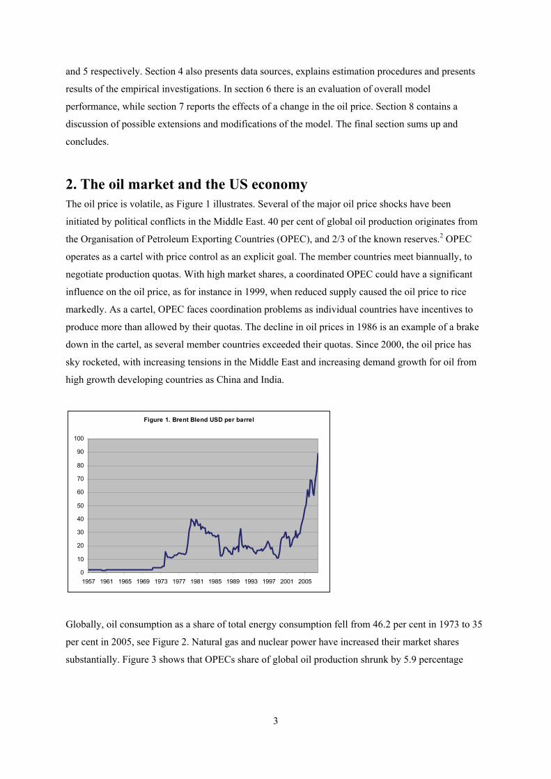
2. The oil market and the US economy The oil price is volatile, as Figure 1 illustrates. Several of the major oil price shocks have been

initiated by political conflicts in the Middle East. 40 per cent of global oil production originates from

the Organisation of Petroleum Exporting Countries (OPEC), and 2/3 of the known reserves.2 OPEC

operates as a cartel with price control as an explicit goal. The member countries meet biannually, to

negotiate production quotas. With high market shares, a coordinated OPEC could have a significant

influence on the oil price, as for instance in 1999, when reduced supply caused the oil price to rice

markedly. As a cartel, OPEC faces coordination problems as individual countries have incentives to

produce more than allowed by their quotas. The decline in oil prices in 1986 is an example of a brake

down in the cartel, as several member countries exceeded their quotas. Since 2000, the oil price has

sky rocketed, with increasing tensions in the Middle East and increasing demand growth for oil from

high growth developing countries as China and India.

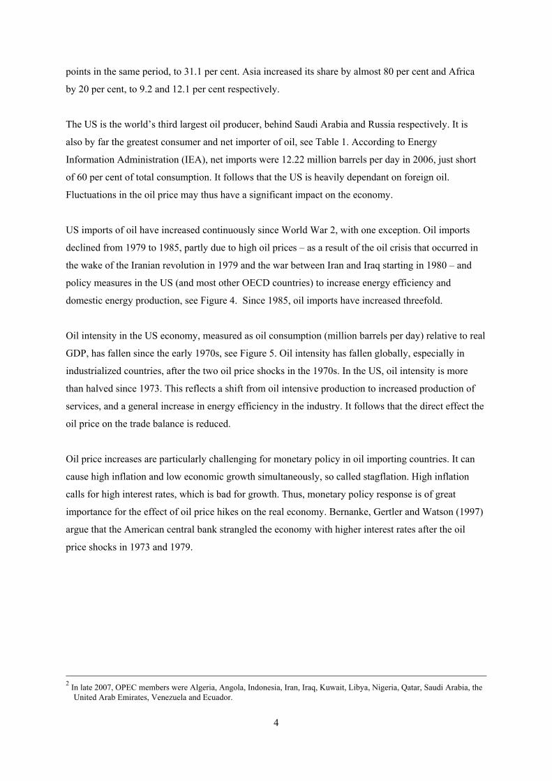
Globally, oil consumption as a share of total energy consumption fell from 46.2 per cent in 1973 to 35

per cent in 2005, see Figure 2. Natural gas and nuclear power have increased their market shares

substantially. Figure 3 shows that OPECs share of global oil production shrunk by 5.9 percentage

Figure 1. Brent Blend USD per barrel

0

10

20

30

40

50

60

70

80

90

100

1957 1961 1965 1969 1973 1977 1981 1985 1989 1993 1997 2001 2005

4

points in the same period, to 31.1 per cent. Asia increased its share by almost 80 per cent and Africa

by 20 per cent, to 9.2 and 12.1 per cent respectively.

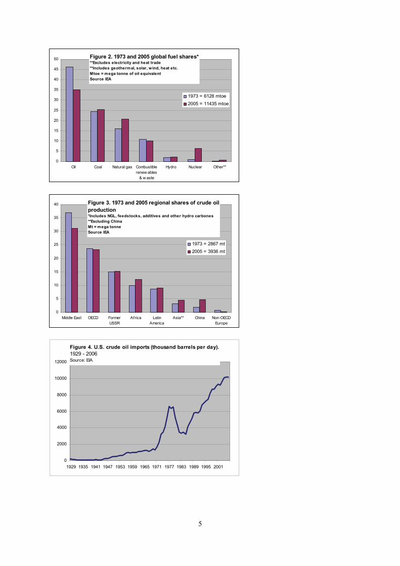
The US is the world’s third largest oil producer, behind Saudi Arabia and Russia respectively. It is

also by far the greatest consumer and net importer of oil, see Table 1. According to Energy

Information Administration (IEA), net imports were 12.22 million barrels per day in 2006, just short

of 60 per cent of total consumption. It follows that the US is heavily dependant on foreign oil.

Fluctuations in the oil price may thus have a significant impact on the economy.

US imports of oil have increased continuously since World War 2, with one exception. Oil imports

declined from 1979 to 1985, partly due to high oil prices – as a result of the oil crisis that occurred in

the wake of the Iranian revolution in 1979 and the war between Iran and Iraq starting in 1980 – and

policy measures in the US (and most other OECD countries) to increase energy efficiency and

domestic energy production, see Figure 4. Since 1985, oil imports have increased threefold.

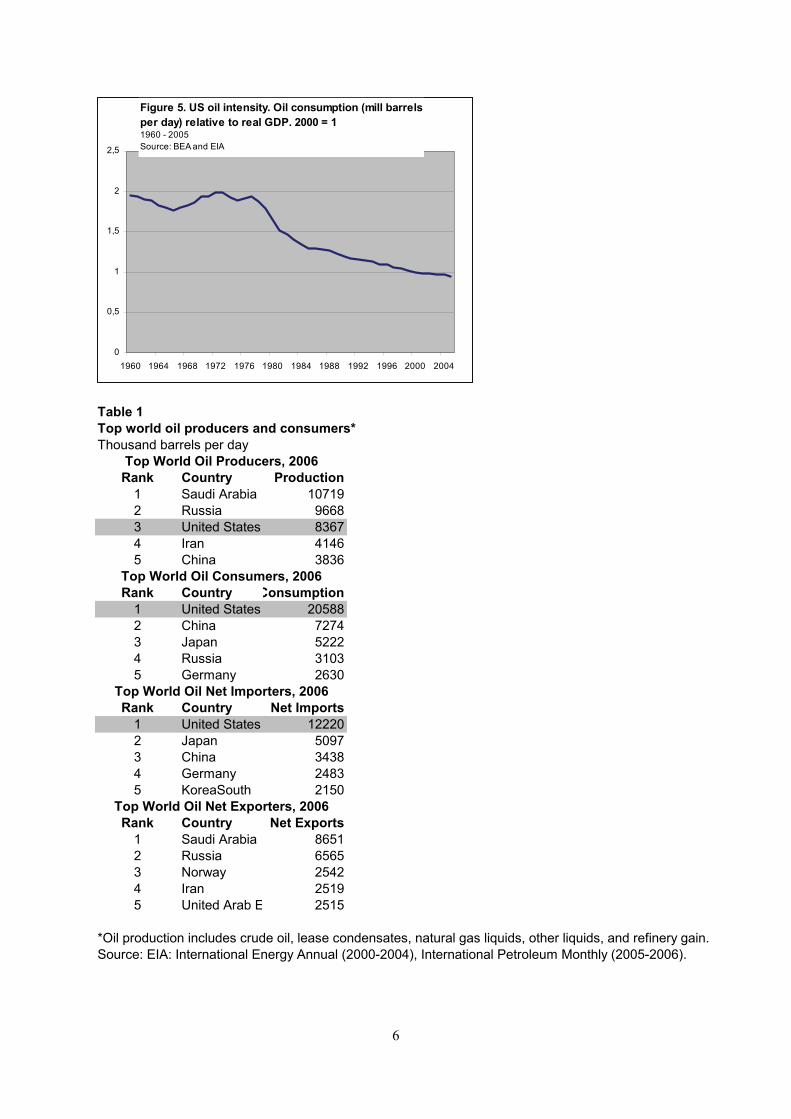
Oil intensity in the US economy, measured as oil consumption (million barrels per day) relative to real

GDP, has fallen since the early 1970s, see Figure 5. Oil intensity has fallen globally, especially in

industrialized countries, after the two oil price shocks in the 1970s. In the US, oil intensity is more

than halved since 1973. This reflects a shift from oil intensive production to increased production of

services, and a general increase in energy efficiency in the industry. It follows that the direct effect the

oil price on the trade balance is reduced.

Oil price increases are particularly challenging for monetary policy in oil importing countries. It can

cause high inflation and low economic growth simultaneously, so called stagflation. High inflation

calls for high interest rates, which is bad for growth. Thus, monetary policy response is of great

importance for the effect of oil price hikes on the real economy. Bernanke, Gertler and Watson (1997)

argue that the American central bank strangled the economy with higher interest rates after the oil

price shocks in 1973 and 1979.

2 In late 2007, OPEC members were Algeria, Angola, Indonesia, Iran, Iraq, Kuwait, Libya, Nigeria, Qatar, Saudi Arabia, the

United Arab Emirates, Venezuela and Ecuador.

5

Figure 4. U.S. crude oil imports (thousand barrels per day).1929 - 2006Source: EIA

0

2000

4000

6000

8000

10000

12000

1929 1935 1941 1947 1953 1959 1965 1971 1977 1983 1989 1995 2001

Figure 3. 1973 and 2005 regional shares of crude oil production*Includes NGL, feedstocks, additives and other hydro carbones**Excluding ChinaMt = mega tonneSource IEA

0

5

10

15

20

25

30

35

40

Middle East OECD FormerUSSR

Africa LatinAmerica

Asia** China Non-OECDEurope

1973 = 2867 mt2005 = 3936 mt

Figure 2. 1973 and 2005 global fuel shares***Excludes electricity and heat trade**Includes geothermal, solar, w ind, heat etc.Mtoe = mega tonne of oil equivalentSource IEA

0

5

10

15

20

25

30

35

40

45

50

Oil Coal Natural gas Combustiblerenew ables

& w aste

Hydro Nuclear Other**

1973 = 6128 mtoe2005 = 11435 mtoe

6

Table 1Top world oil producers and consumers*Thousand barrels per day

Rank Country Production1 Saudi Arabia 107192 Russia 96683 United States 83674 Iran 41465 China 3836

Rank Country Consumption1 United States 205882 China 72743 Japan 52224 Russia 31035 Germany 2630

Rank Country Net Imports1 United States 122202 Japan 50973 China 34384 Germany 24835 KoreaSouth 2150

Rank Country Net Exports1 Saudi Arabia 86512 Russia 65653 Norway 25424 Iran 25195 United Arab E 2515

*Oil production includes crude oil, lease condensates, natural gas liquids, other liquids, and refinery gain. Source: EIA: International Energy Annual (2000-2004), International Petroleum Monthly (2005-2006).

Top World Oil Producers, 2006

Top World Oil Consumers, 2006

Top World Oil Net Exporters, 2006

Top World Oil Net Importers, 2006

Figure 5. US oil intensity. Oil consumption (mill barrels per day) relative to real GDP. 2000 = 11960 - 2005Source: BEA and EIA

0

0,5

1

1,5

2

2,5

1960 1964 1968 1972 1976 1980 1984 1988 1992 1996 2000 2004

7

3. Model description

The model of the US economy, hereby referred to as the US model, is a macro econometric model.

The model is simple compared to large scale macro econometric models like for instance National

Institute of Economic and Social Research’s NIGEM model (Barrel et al 2001)3, Ray C. Fair’s US

model (Fair 2004) and Statistics Norway’s MODAG (Baug et al 2004), and more in line with the small

scale country models in Fair’s global model (Fair 2004) and the Norwegian Aggregate Model (NAM)

(cf. Nymoen 2008).

The US model contains 9 estimated equations, and a number of identities. Household consumption,

private domestic investment, exports and imports are modelled econometrically. Government

expenditure is determined outside the model. Real GDP follows as the sum of domestic demand and

net exports. Furthermore, there are estimated equations for consumer prices and the GDP deflator, and

three equations describing the labour market. The model facilitates analyses of, among other things,

effects on the economy of changes in interest rates, government expenditure, international demand and

prices – including the oil price.

4. Data and estimation The model is estimated on annual data, to serve FRISBEE. National accounts data are from Bureau of

economic Analyses. Labour market data and data for interest rates, household wealth and household

income are from the Fair model data base. The oil price and data for the G7 countries are from OECD

Economic Outlook and OECD Main Economic Indicators. Se Appendix A for details.

The software EViews6 is used for all estimation and simulation procedures. The estimation periods

were chosen based on data availability. The shortest time series (the GDP deflator for the G7

countries) begins in 1970. Because of dynamics, simulation of the full model can start in 1973.

The modeling strategy is the general to specific approach (cf. Davidson et al (1978)), using ordinary

least squares to estimate equilibrium correction models. Restrictions based on economic theory are

applied when statistical support is found. Other parameter restrictions are implemented if contributing

to simplify the model without reducing the fit. It is also emphasized that the final estimated equations

should pass standard statistical tests for serial correlation, heteroscedasticity and normality in the

residuals. Parameter stability is tested through recursive estimation. Statistical outliers are removed by

impulse dummies if explainable and/or if substantial improvement in residual properties are achieved.

3 See also http://www.niesr.ac.uk/research/research.php#1

8

D is a difference operator when appearing in front of a variable name (DXt = Xt-Xt-1). Dyyt represents

an impulse dummy variable for year yy. Ui is the error term in Equation i = 1,2,…,9.

In all estimated equations the coefficient relating to the equilibrium correction term is significant with

the right sign, indicating a cointegrating relationship between the variables in the long run.

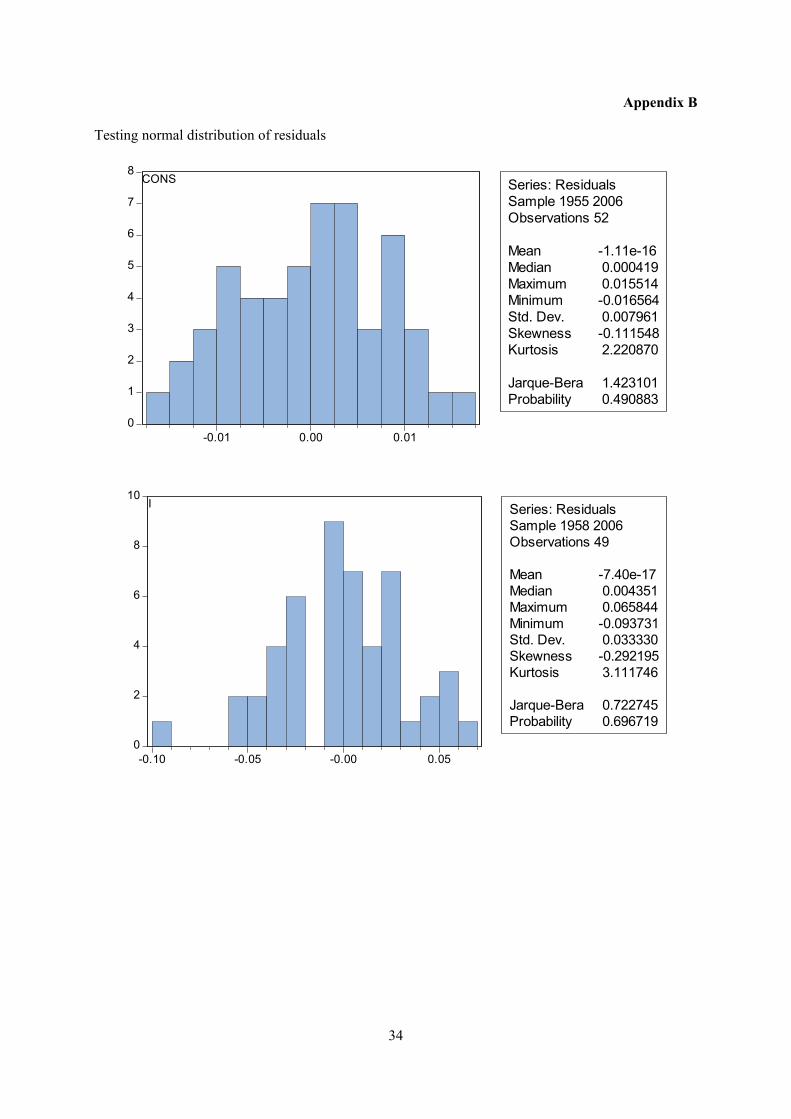
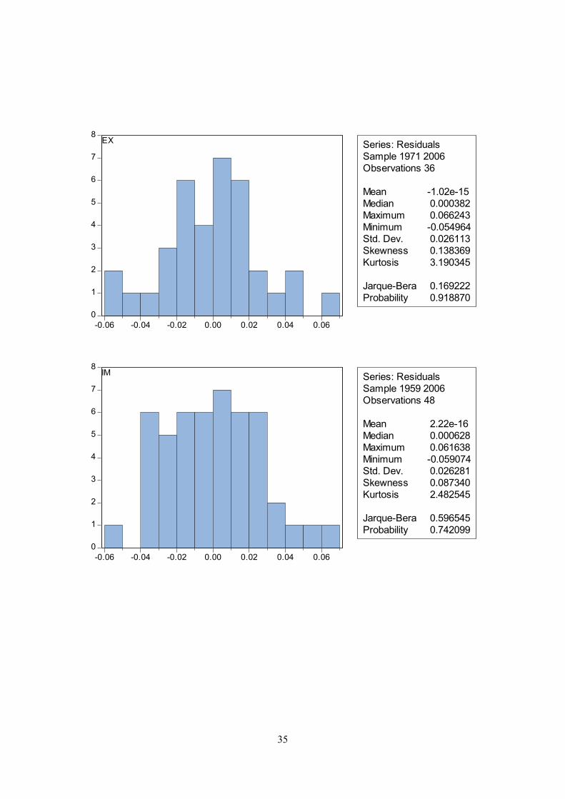
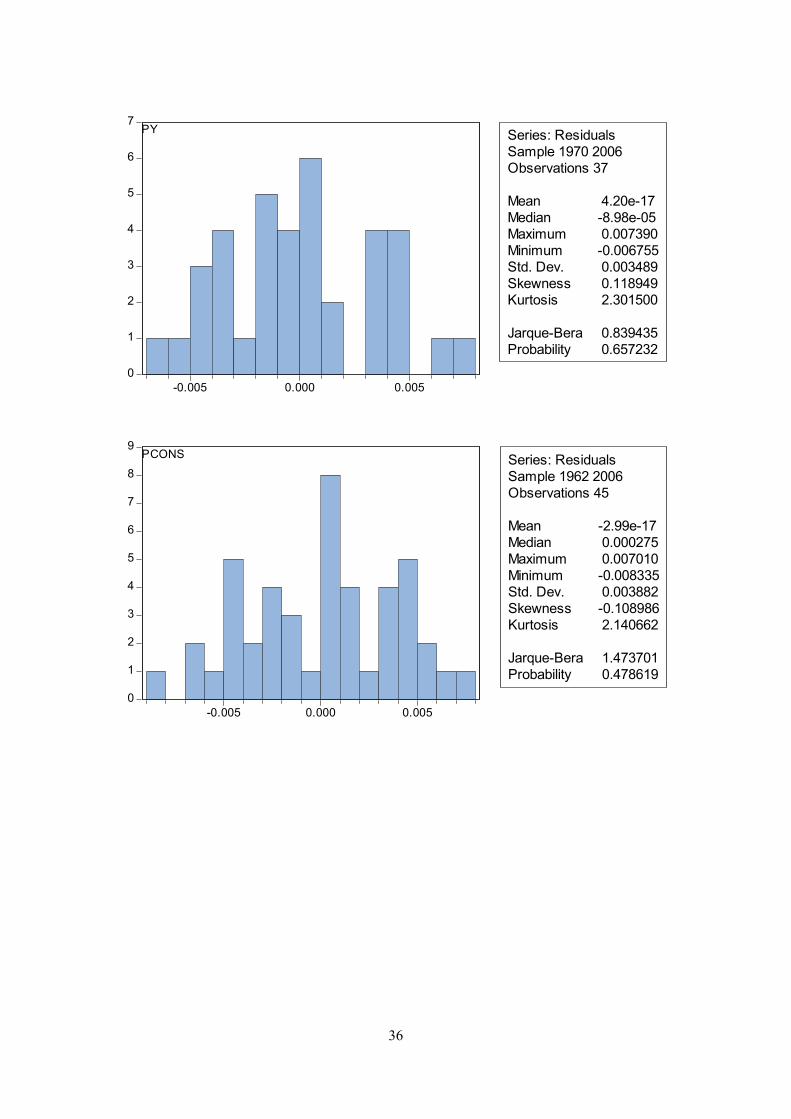
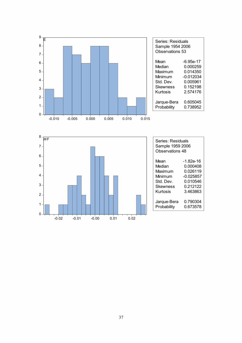
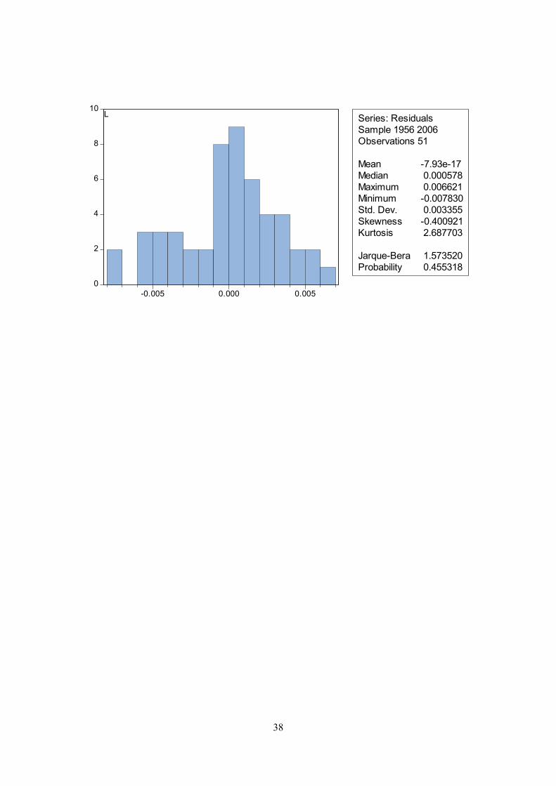
The assumption of normal distribution of the residuals is tested. The null hypothesis of normal

distribution is not rejected for any of the equations at the five per cent level. A histogram and the

Jarque-Bera statistic are reported in appendix B.

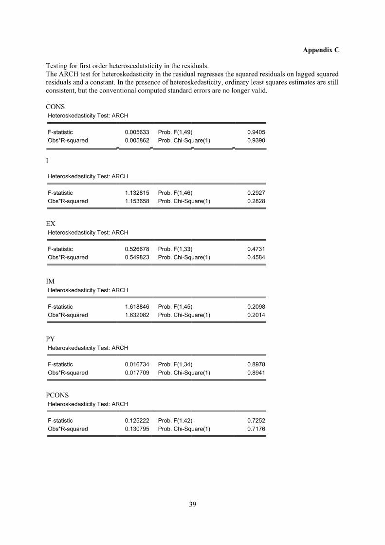
The ARCH test for heteroskedasticity in the residual regresses the squared residuals on lagged squared

residuals and a constant. In the presence of heteroskedasticity, ordinary least squares estimates are still

consistent, but the conventional computed standard errors are no longer valid. Heteroscedasticity does

not appear to pose a problem in any of the equations, with the possible exception of the equation for

employment (E), where the null hypothesis of no heteroskedasticity is rejected on the five per cent

level, but not on the 1 per cent level, see appendix C.

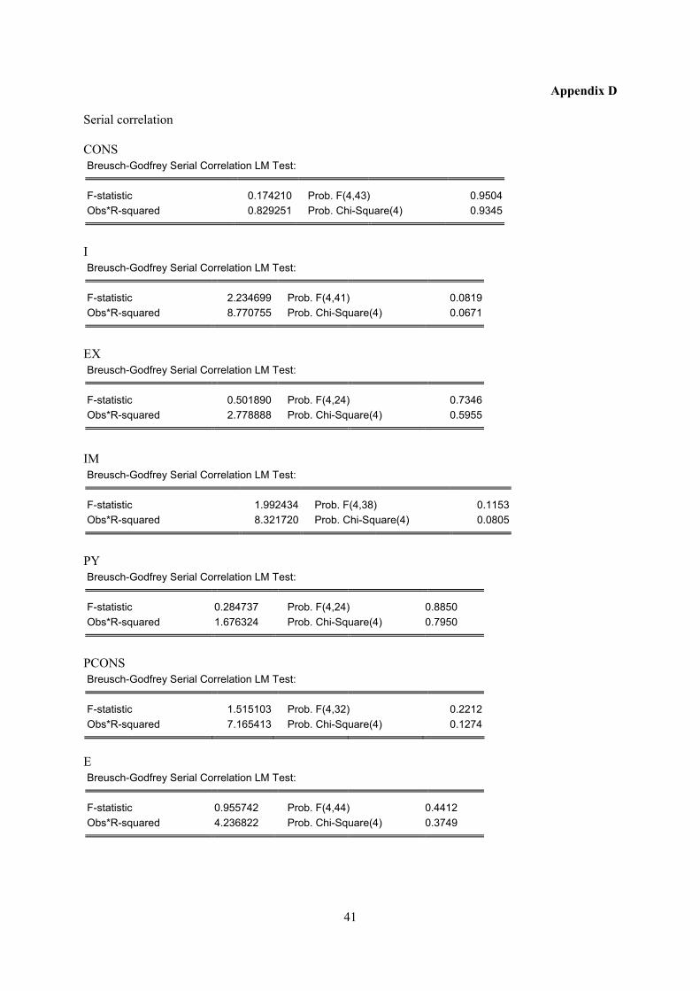
If the error term is serially correlated, the estimated OLS standard errors are invalid and the estimated

coefficients will be biased and inconsistent due to the presence of a lagged dependent variable on the

right-hand side. The Durbin-Watson statistic is not appropriate as a test for serial correlation when

there is a lagged dependent variable on the right-hand side of the equation. The Breusch-Godfrey LM-

test does not reject the null hypothesis of no serial correlation up to order four for any of the equations

at the five per cent level, see appendix D.

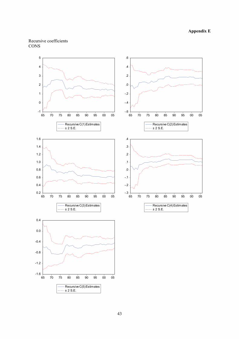
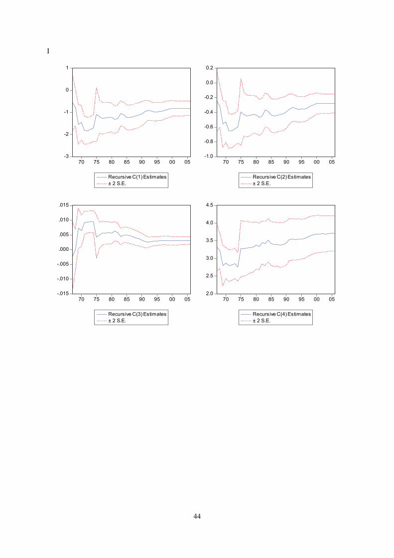
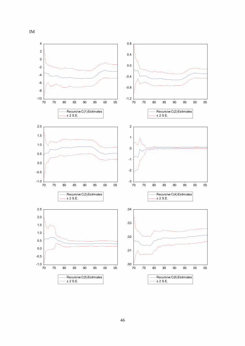
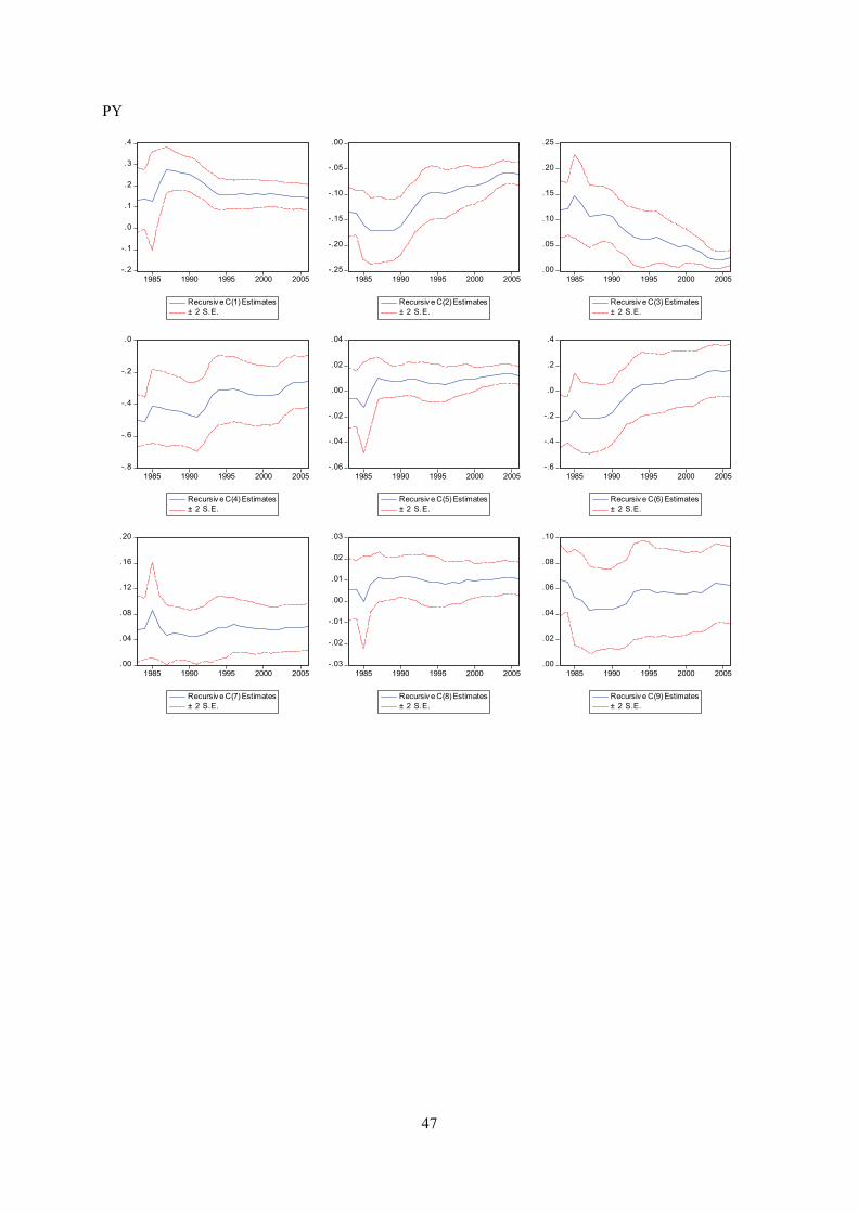
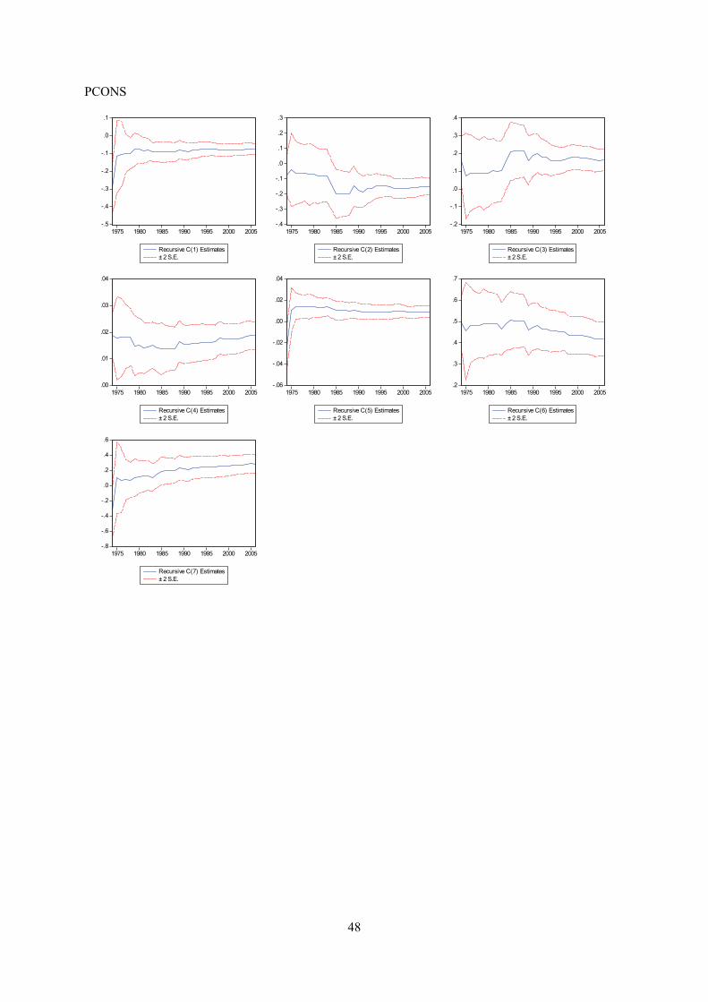
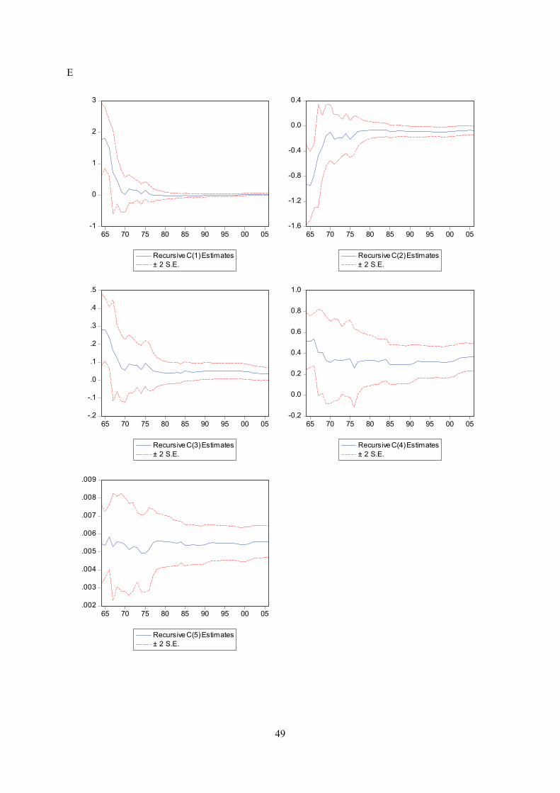
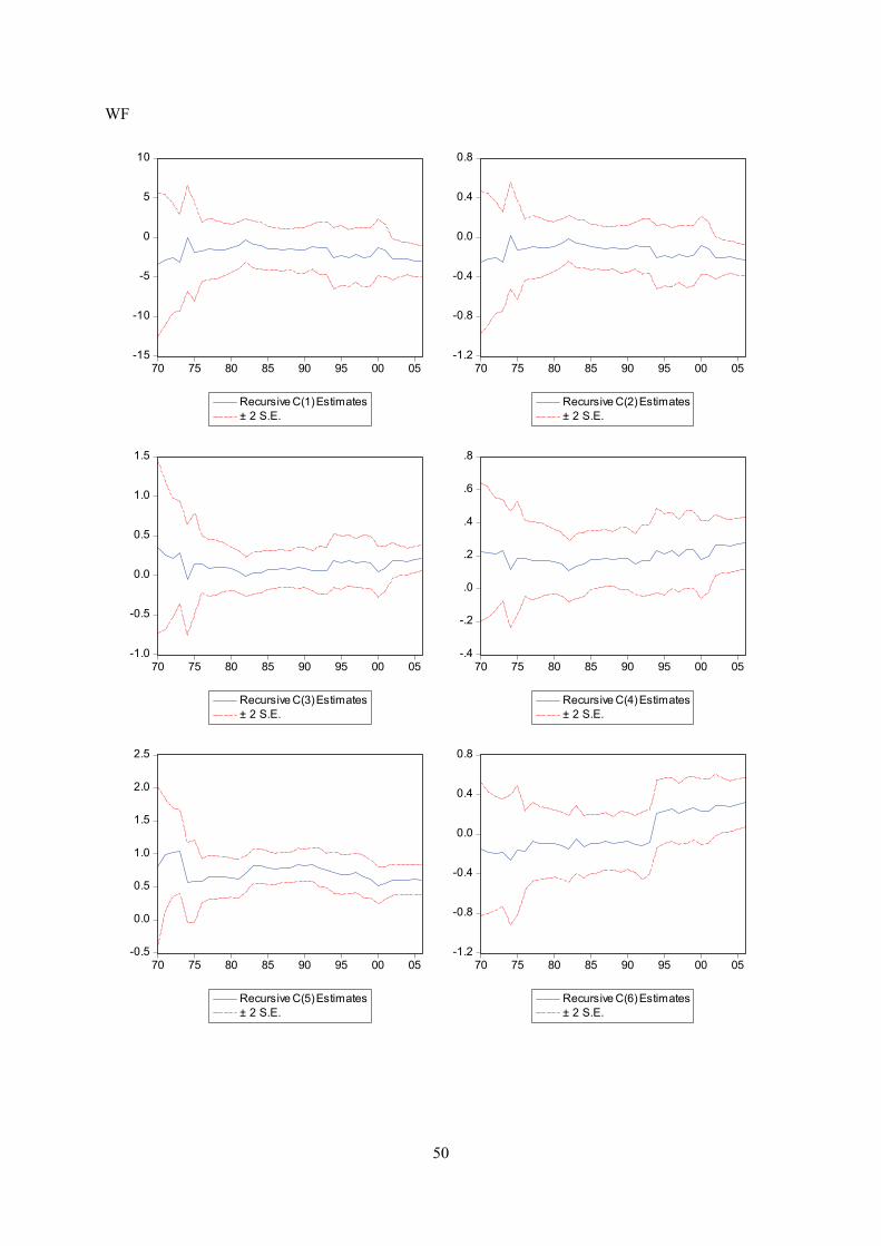
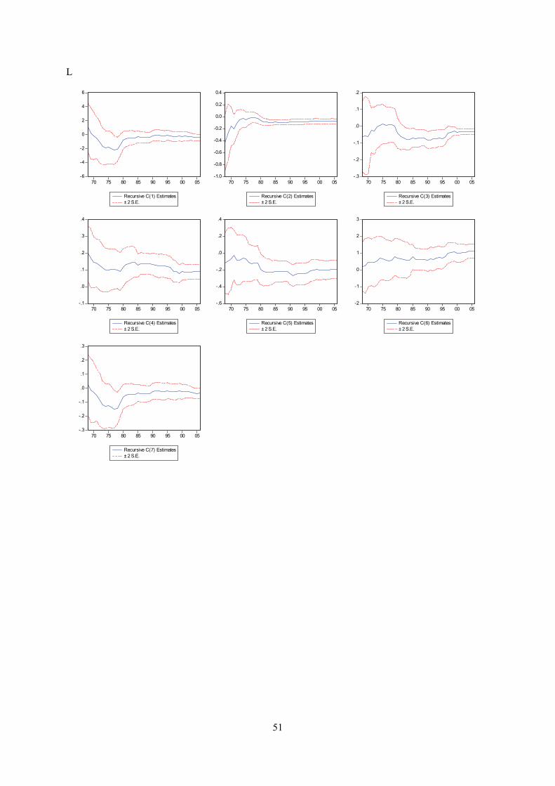
Appendix E displays recursive coeffisient estimates. They enable you to trace the evolution of

estimates for a coefficient as an increasing number of observations are used in the estimation. Two

standard error bands around the estimated coefficients are also shown. If the coefficient displays

significant variation as more data is added, it is a strong indication of instability. In both trade

equations there are indications of a structural break in the second half of the 1990’s. Impulse- and step

dummy variables did not do the trick on either occasion, although an impulse dummy in the export

equation reduced the problem. However, recursive estimation of the residuals does not indicate

instability (see below). As for the other equations, recursive coefficient estimates reveal no major

cause for concern.

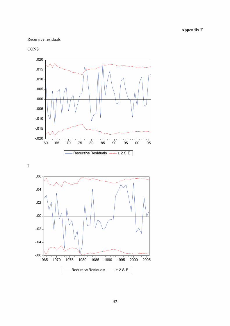
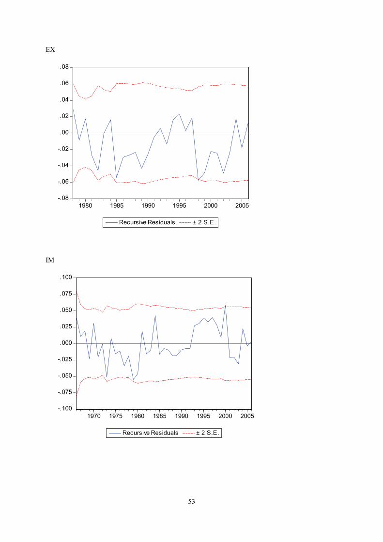
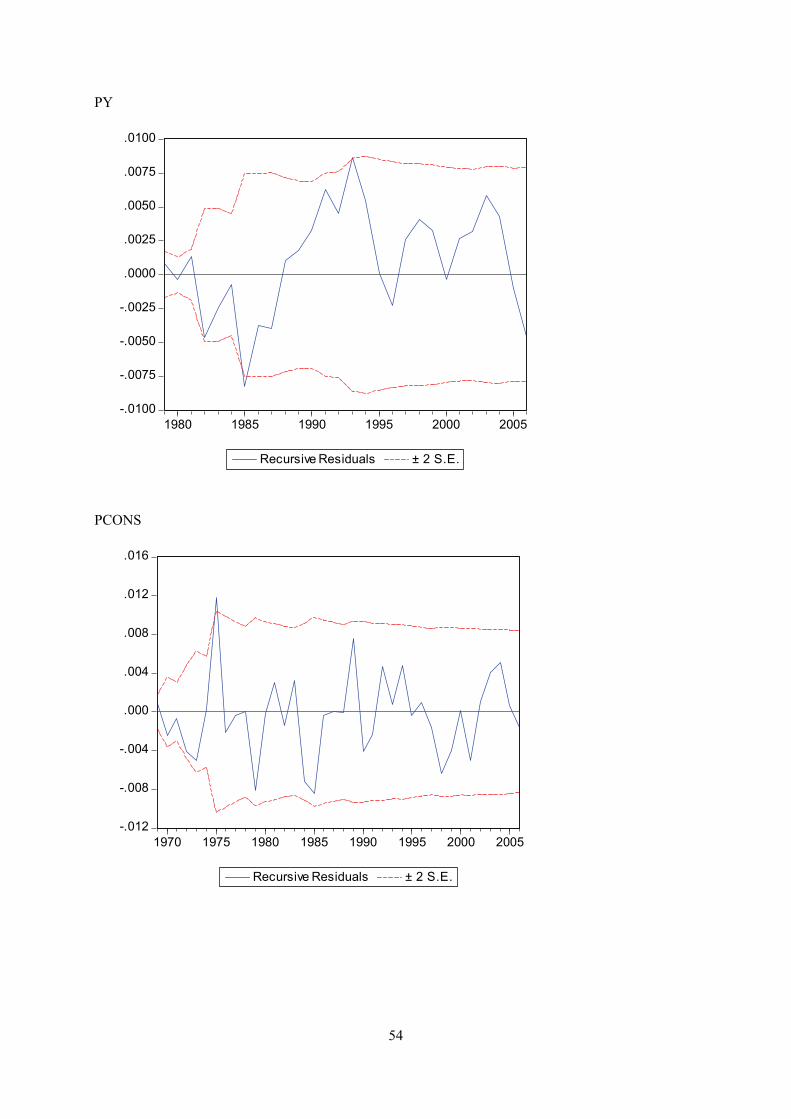
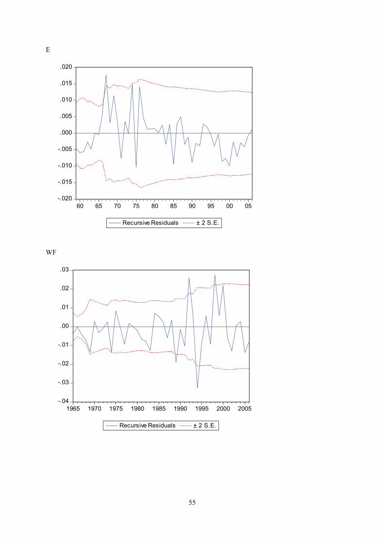
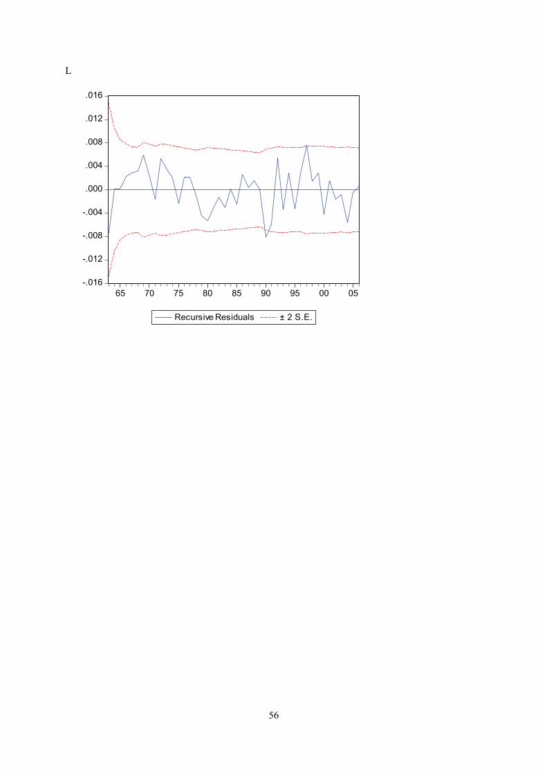
Appendix F displays plots of recursive residuals for each equation. Plus/minus two standard errors are

shown at each point. Residuals outside the standard error bands would suggest instability in the

9

equation parameters. At the 5 per cent level, 5 observations out of 100 outside the error band are

acceptable. This test does not give strong indications of instability for any of the equations.

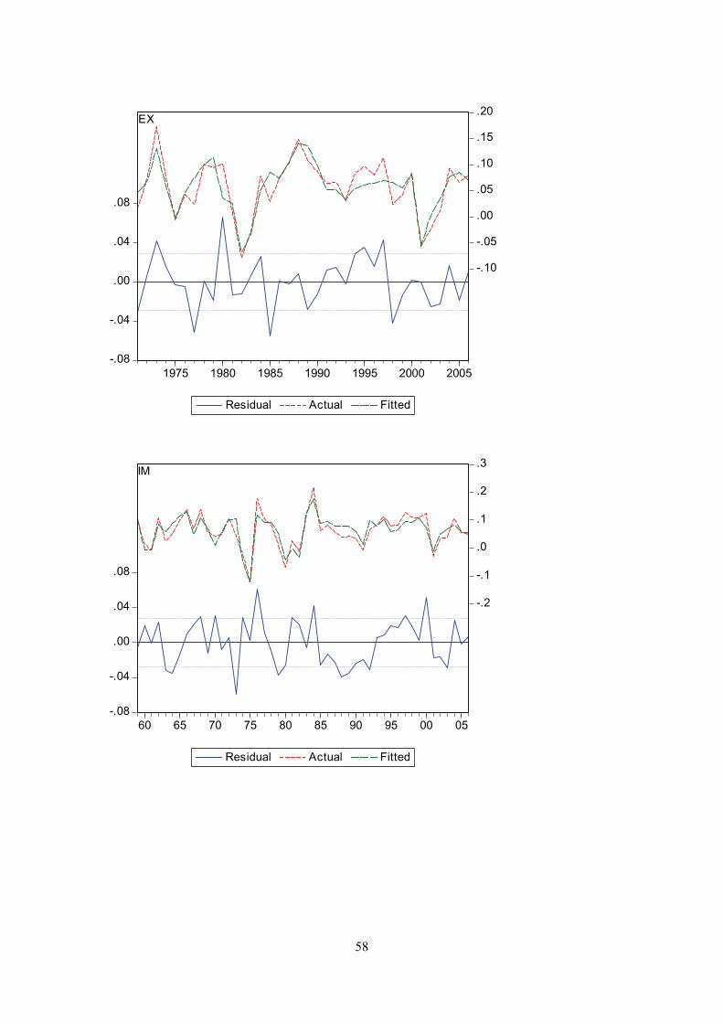
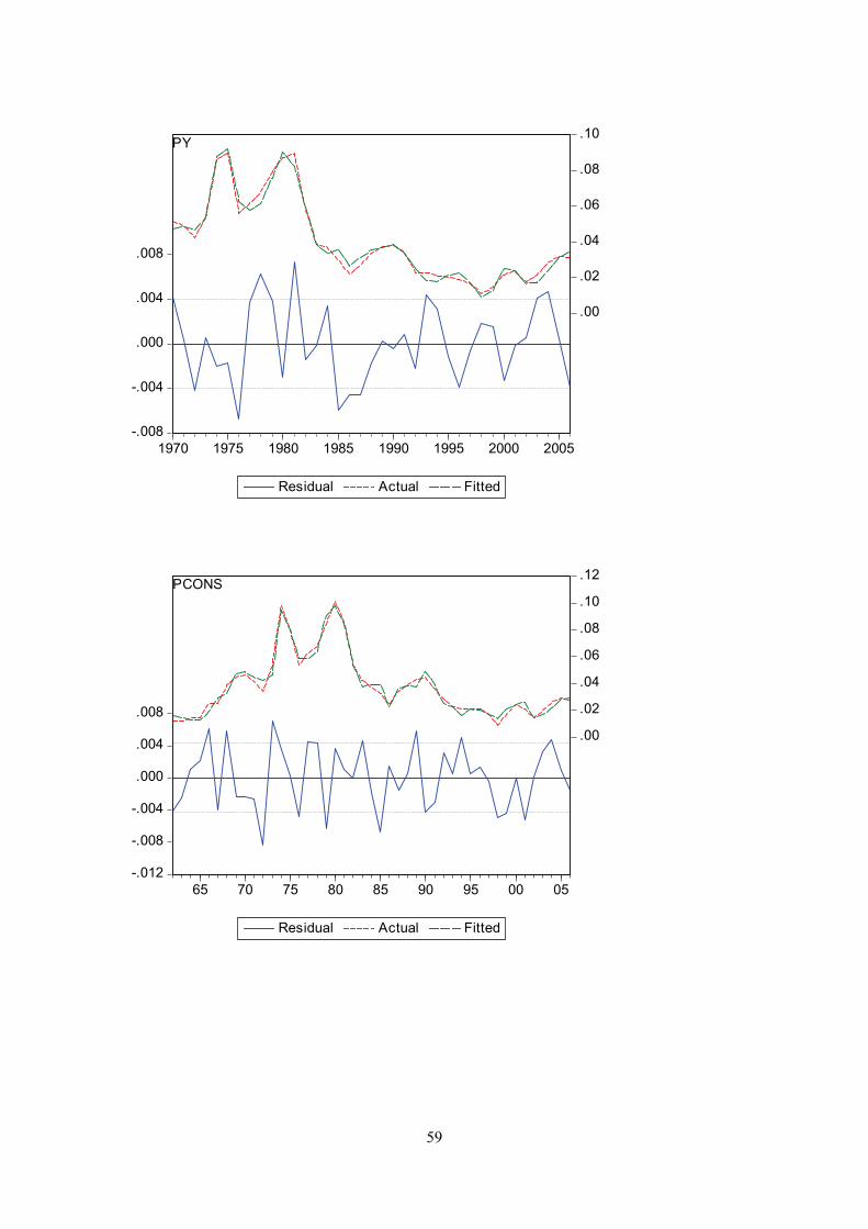
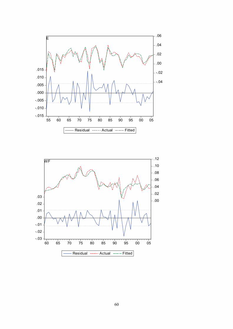
Estimation results for the nine equations are discussed below. Regression output and test statistics

reported with each equation are briefly explained in Box 1. Appendix G displays actual and fitted

values of the dependent variable and the residuals from the regression for each equation.

Box1. Regression output and test statistics The R-squared (R2) statistic measures the success of the regression in predicting the values of the dependent variable within the sample. The statistic will equal one if the regression fits perfectly, and zero if it fits no better than the simple mean of the dependent variable. The adjusted R2 penalizes the R2 for the addition of regressors which do not contribute to the explanatory power of the model. The standard error (S.E.) of the regression is a summary measure based on the estimated variance of the residuals. The Durbin-Watson (DW) is a test for first order serial correlation in the residuals. As a rule of thumb, if the DW is less than 2, there is evidence of positive serial correlation. if there are lagged dependent variables on the right-hand side of the regression, the DW test is no longer valid. Additional testing of serial correlation is reported in appendix D. The Akaike-, Schwarz- and Hannan-Quinn information criteria provide measures of information that strikes a balance goodness of fit and parsimonious specification of the model, and are used as a guides in model selection. The F-statistic reported in the regression output is from a test of the hypothesis that all of the slope coefficients (excluding the constant, or intercept) in a regression are zero. The Prob(F-statistic) shows the probability of drawing a t-statistic (or a z-statistic) as extreme as the one actually observed, under the assumption that the errors are normally distributed, or that the estimated coefficients are asymptotically normally distributed. The Table also shows the mean and the standard deviation of the endogenous (dependent) variable.

10

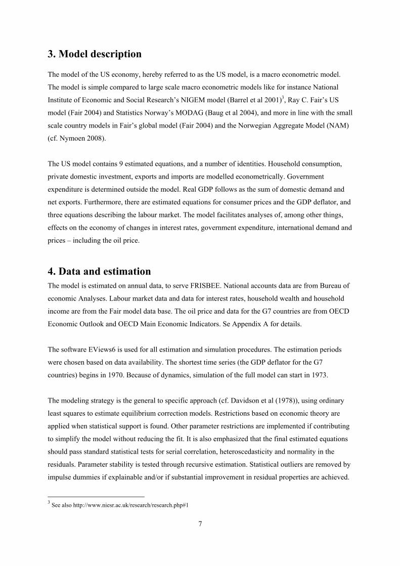
Equation 1, CONS = household consumption expenditure Dependent Variable: D(LOG(CONS)) Method: Least Squares Sample: 1955 2006 Included observations: 52

Coefficient Std. Error t-Statistic Prob.

C 1.299773 0.302629 4.294932 0.0001 D(LOG(CONS(-1))) 0.144095 0.077106 1.868788 0.0679

D(LOG(YD)-LOG(PCONS)) 0.623112 0.079766 7.811766 0.0000 D(LOG(AA))-D(LOG(AA(-2))) 0.101161 0.021837 4.632584 0.0000

CIC(-1)* -0.426326 0.099820 -4.270940 0.0001

R-squared 0.771139 Mean dependent var 0.035177 Adjusted R-squared 0.751661 S.D. dependent var 0.016641 S.E. of regression 0.008293 Akaike info criterion -6.655631 Sum squared resid 0.003232 Schwarz criterion -6.468011 Log likelihood 178.0464 Hannan-Quinn criter. -6.583702 F-statistic 39.59114 Durbin-Watson stat 1.942561 Prob(F-statistic) 0.000000

*CIC = LOG(CONS) -0.247226 * LOG(AA) +0.00129085 * RSS -0.752774 * (LOG(YD)-LOG(PCONS)) -0.00128515 * TREND

Household consumption expenditure (CONS) is modelled in Equation 1. In the long run, a one per

cent increase in real disposable income (YD/PCONS) and wealth (AA) will, all else equal, lead to a 1

per cent increase in household consumption of 1 per cent – consumption is homogenous of degree one

in real disposable income and wealth. There is also a negative long run effect of the real interest rate

(RSS) on consumption. Thus, monetary policy has a direct effect on consumption through the interest

rate. There are positive short run effects of real disposable income and (accelerating) wealth.4

4 Equation 1 was derived using the multivariate cointegration procedure proposed by Johansen (1988), and estimated in Pc

Give (cf. Hendry and Doornik 2001).

11

Equation 2, I = gross domestic investment

Dependent Variable: D(LOG(I)) Method: Least Squares Sample: 1958 - 2006 Included observations: 49


C -0.815245 0.160187 -5.089320 0.0000LOG(I(-1))-LOG(Y(-1)) -0.278930 0.063972 -4.360166 0.0001

T 0.003122 0.000654 4.772923 0.0000D(LOG(Y)) 3.710622 0.246474 15.05481 0.0000

R-squared 0.861312 Mean dependent var 0.042288Adjusted R-squared 0.852066 S.D. dependent var 0.089499S.E. of regression 0.034423 Akaike info criterion -3.822057Sum squared resid 0.053323 Schwarz criterion -3.667622Log likelihood 97.64039 Hannan-Quinn criter. -3.763464F-statistic 93.15623 Durbin-Watson stat 1.778381Prob(F-statistic) 0.000000

Gross domestic investments (I) depend positively on output (Y) in the long run. Increasing output

leads to increasing demand for production capacity, as well as increased depreciation of capital, both

inducing higher investments. A one per cent increase in output leads to a one per cent increase in

investment per restriction. This homogeneity restriction is tested and not rejected. The statistical

validity of the restriction depends on the inclusion of a deterministic trend (T), taking account of the

fact that investments has grown more rapidly than GDP over time.

12

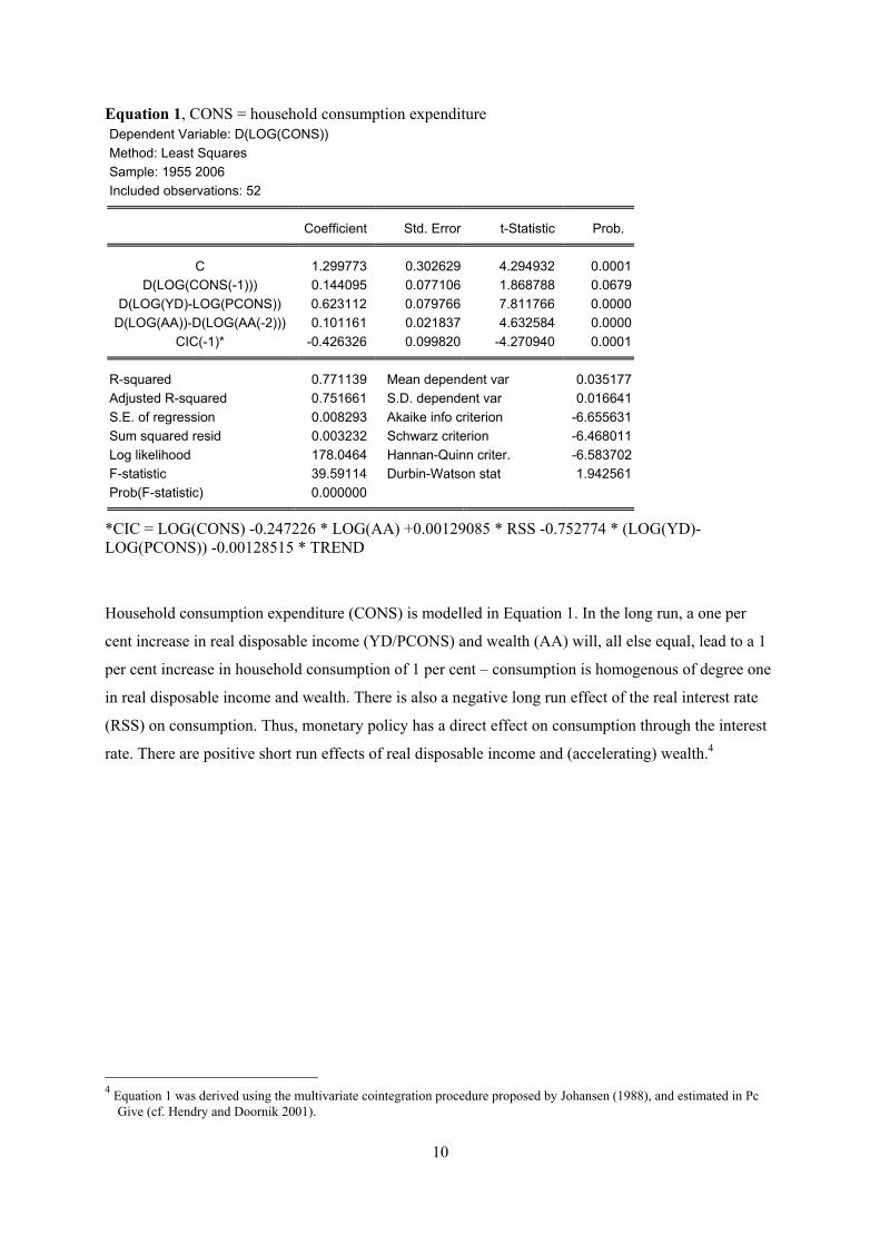
Equation 3, EX = exports Dependent Variable: D(LOG(EX)) Method: Least Squares Sample (adjusted): 1971 2006 Included observations: 36 after adjustments


C -1.121487 0.294684 -3.805732 0.0007LOG(EX(-1)) -0.208785 0.069645 -2.997846 0.0056LOG(PY(-1)) -0.923946 0.418017 -2.210308 0.0354

LOG(PYG7(-1)) 0.620219 0.314695 1.970862 0.0587LOG(YG7(-1)) 0.862354 0.244082 3.533048 0.0014

D(LOG(EX(-1))) 0.392370 0.102559 3.825794 0.0007D(LOG(YG7)) 2.168593 0.381260 5.687957 0.0000

D01 -0.100649 0.031249 -3.220834 0.0032


Equation 3 explains exports (EX). International demand (Y7) and international prices (PY7) are

proxied by GDP and the GDP deflator for the G7 countries respectively. The GDP deflator (PY)

replaces the export price, which was not significant. In the long run exports depend positively on

international demand an international prices and negatively on domestic prices. This is in line with the

standard export model proposed by Armington (1969). Price homogeneity is not rejected by the

standard errors. However, if this restriction is imposed explicitly, the cointegrating relationship

between the variables breaks down. There are positive short run effects of international demand.

13

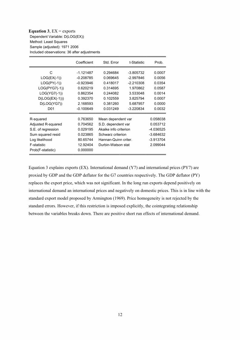
Equation 4, IM = imports Dependent Variable: D(LOG(IM)) Method: Least Squares Sample: 1959 - 2006 Included observations: 48


C -2.980034 0.869934 -3.425584 0.0014 LOG(IM(-1)) -0.279478 0.081846 -3.414663 0.0014

LOG((CONS(-1)+G(-1)+I(-1))) 0.548627 0.158117 3.469763 0.0012 LOG(PY(-1)/PIM(-1)) 0.098175 0.036744 2.671909 0.0107

D(LOG(PY(-1)/PIM(-1))) 0.324715 0.079323 4.093551 0.0002 D(YGAP) 0.021409 0.002380 8.994420 0.0000

R-squared 0.810428 Mean dependent var 0.063323 Adjusted R-squared 0.787860 S.D. dependent var 0.060360 S.E. of regression 0.027801 Akaike info criterion -4.211022 Sum squared resid 0.032462 Schwarz criterion -3.977122 Log likelihood 107.0645 Hannan-Quinn criter. -4.122631 F-statistic 35.91036 Durbin-Watson stat 1.724719 Prob(F-statistic) 0.000000

Equation 4 explains imports (IM) as a function of domestic demand and relative prices. Increased

domestic demand leads to increased imports. If domestic prices increase relative to prices on imported

goods and services - all else being equal - imports will increase. Domestic demand is represented by

the sum of household consumption (CONS), government consumption and investment (G) and private

investment (I), implying identical marginal import elasticity for all variables. This restriction is tested

and not rejected. PIM is the import price. A domestic price deflator was calculated by weighing

together the deflators for household consumption, private investment and government consumption

and investment, but the GDP-deflator proved a better alternative due to superior statistical

performance. There are also positive short run effects of relative prices and domestic economic

activity. Price homogeneity was tested and not rejected, both in the long and the short run.

14

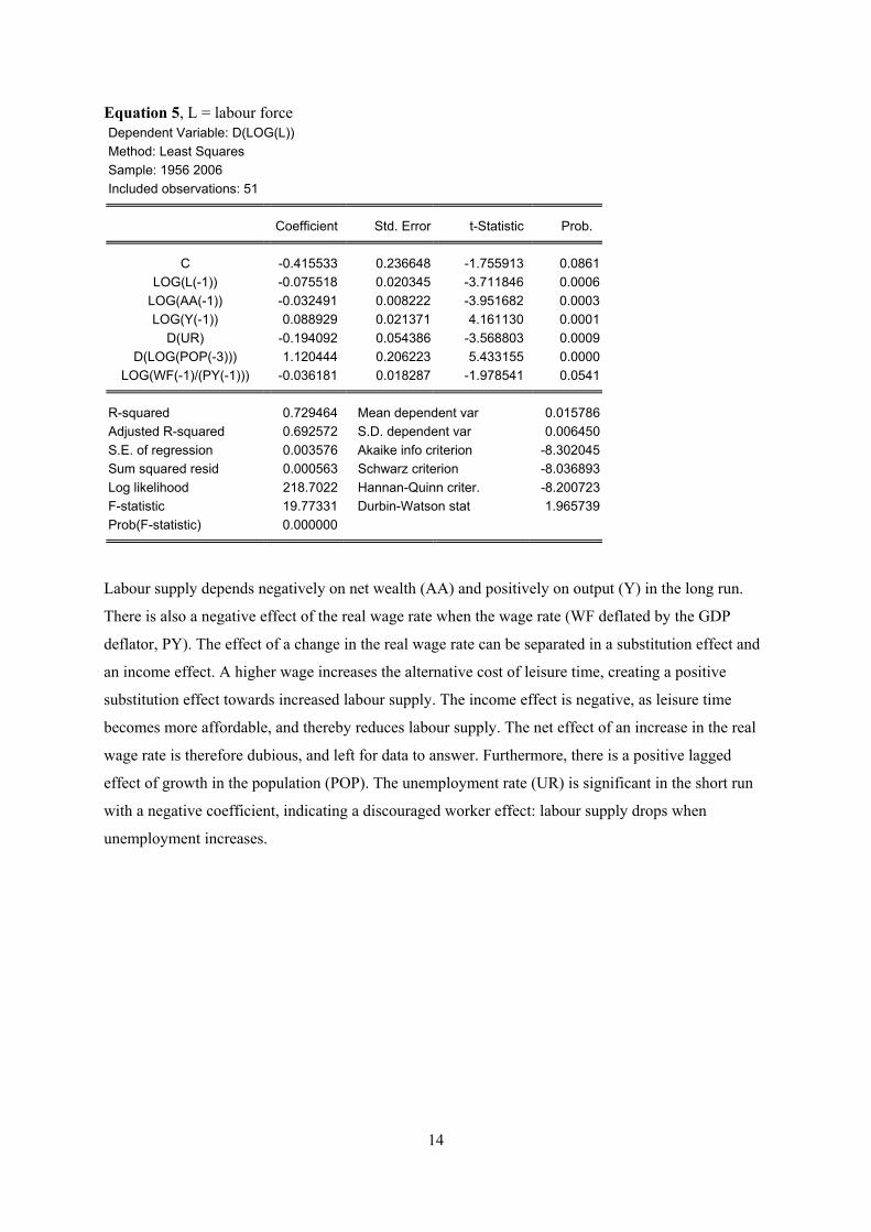
Equation 5, L = labour force Dependent Variable: D(LOG(L)) Method: Least Squares Sample: 1956 2006 Included observations: 51


C -0.415533 0.236648 -1.755913 0.0861LOG(L(-1)) -0.075518 0.020345 -3.711846 0.0006

LOG(AA(-1)) -0.032491 0.008222 -3.951682 0.0003LOG(Y(-1)) 0.088929 0.021371 4.161130 0.0001

D(UR) -0.194092 0.054386 -3.568803 0.0009D(LOG(POP(-3))) 1.120444 0.206223 5.433155 0.0000

LOG(WF(-1)/(PY(-1))) -0.036181 0.018287 -1.978541 0.0541


Labour supply depends negatively on net wealth (AA) and positively on output (Y) in the long run.

There is also a negative effect of the real wage rate when the wage rate (WF deflated by the GDP

deflator, PY). The effect of a change in the real wage rate can be separated in a substitution effect and

an income effect. A higher wage increases the alternative cost of leisure time, creating a positive

substitution effect towards increased labour supply. The income effect is negative, as leisure time

becomes more affordable, and thereby reduces labour supply. The net effect of an increase in the real

wage rate is therefore dubious, and left for data to answer. Furthermore, there is a positive lagged

effect of growth in the population (POP). The unemployment rate (UR) is significant in the short run

with a negative coefficient, indicating a discouraged worker effect: labour supply drops when

unemployment increases.

15

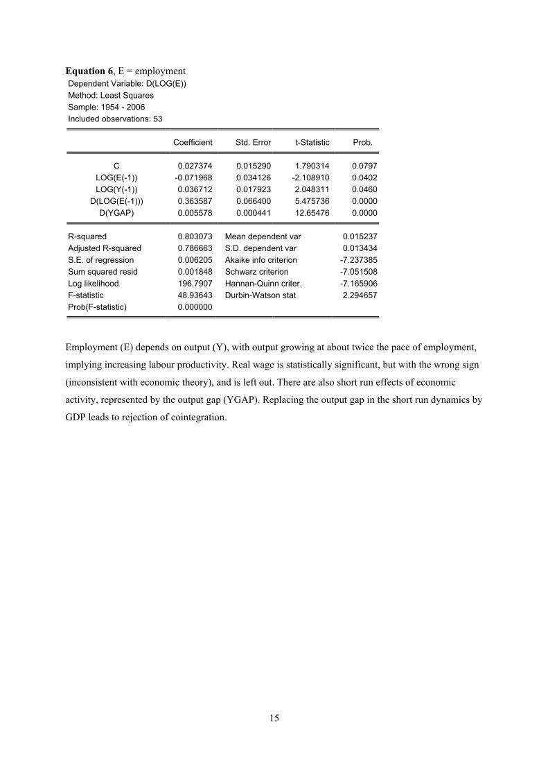
Equation 6, E = employment Dependent Variable: D(LOG(E)) Method: Least Squares Sample: 1954 - 2006 Included observations: 53


C 0.027374 0.015290 1.790314 0.0797LOG(E(-1)) -0.071968 0.034126 -2.108910 0.0402LOG(Y(-1)) 0.036712 0.017923 2.048311 0.0460

D(LOG(E(-1))) 0.363587 0.066400 5.475736 0.0000D(YGAP) 0.005578 0.000441 12.65476 0.0000


Employment (E) depends on output (Y), with output growing at about twice the pace of employment,

implying increasing labour productivity. Real wage is statistically significant, but with the wrong sign

(inconsistent with economic theory), and is left out. There are also short run effects of economic

activity, represented by the output gap (YGAP). Replacing the output gap in the short run dynamics by

GDP leads to rejection of cointegration.

16

Equation 7, WF = average wage per hour Dependent Variable: D(LOG(WF)) Method: Least Squares Sample: 1959 - 2006 Included observations: 48


C -3.033607 1.010480 -3.002145 0.0046LOG(WF(-1)) -0.230776 0.079572 -2.900210 0.0060LOG(PY(-1)) 0.215937 0.082322 2.623080 0.0122

LOG(Y(-1)/E(-1)) 0.274614 0.079911 3.436485 0.0014D(LOG(PY)) 0.607988 0.118001 5.152402 0.0000

D(LOG(WF(-1))) 0.324156 0.131698 2.461355 0.0181D93 -0.037425 0.012071 -3.100528 0.0035


In the long run, average wage per hour (WF) is determined by the GDP-deflator (PY) and

productivity. Productivity is measured by production per employed (Y/E). There are also short run

effects of the GDP deflator and wage. An impulse dummy for 1993 (D93) is included in the equation,

without which homoscedasticity of the residual is rejected.

17

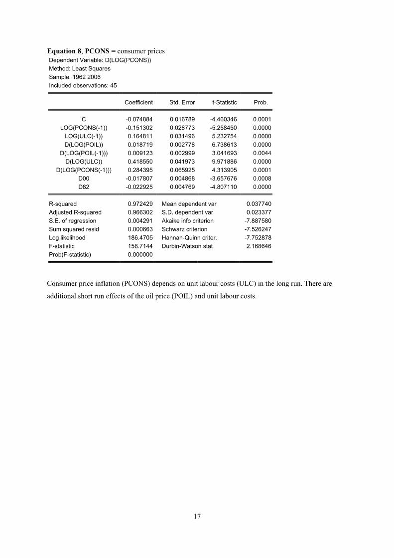
Equation 8, PCONS = consumer prices Dependent Variable: D(LOG(PCONS)) Method: Least Squares Sample: 1962 2006 Included observations: 45


C -0.074884 0.016789 -4.460346 0.0001LOG(PCONS(-1)) -0.151302 0.028773 -5.258450 0.0000

LOG(ULC(-1)) 0.164811 0.031496 5.232754 0.0000D(LOG(POIL)) 0.018719 0.002778 6.738613 0.0000

D(LOG(POIL(-1))) 0.009123 0.002999 3.041693 0.0044D(LOG(ULC)) 0.418550 0.041973 9.971886 0.0000

D(LOG(PCONS(-1))) 0.284395 0.065925 4.313905 0.0001D00 -0.017807 0.004868 -3.657676 0.0008D82 -0.022925 0.004769 -4.807110 0.0000


Consumer price inflation (PCONS) depends on unit labour costs (ULC) in the long run. There are

additional short run effects of the oil price (POIL) and unit labour costs.

18

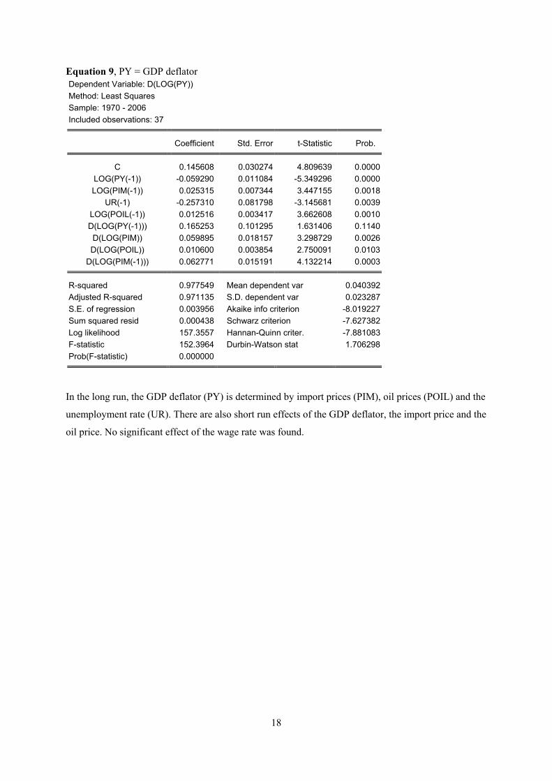
Equation 9, PY = GDP deflator Dependent Variable: D(LOG(PY)) Method: Least Squares Sample: 1970 - 2006 Included observations: 37


C 0.145608 0.030274 4.809639 0.0000LOG(PY(-1)) -0.059290 0.011084 -5.349296 0.0000LOG(PIM(-1)) 0.025315 0.007344 3.447155 0.0018

UR(-1) -0.257310 0.081798 -3.145681 0.0039LOG(POIL(-1)) 0.012516 0.003417 3.662608 0.0010D(LOG(PY(-1))) 0.165253 0.101295 1.631406 0.1140D(LOG(PIM)) 0.059895 0.018157 3.298729 0.0026D(LOG(POIL)) 0.010600 0.003854 2.750091 0.0103

D(LOG(PIM(-1))) 0.062771 0.015191 4.132214 0.0003


In the long run, the GDP deflator (PY) is determined by import prices (PIM), oil prices (POIL) and the

unemployment rate (UR). There are also short run effects of the GDP deflator, the import price and the

oil price. No significant effect of the wage rate was found.

19

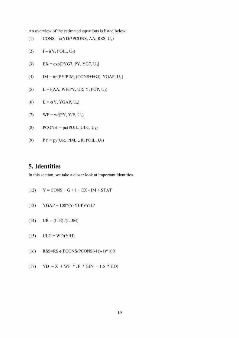
An overview of the estimated equations is listed below:

(1) CONS = c(YD/*PCONS, AA, RSS, U1)

(2) I = i(Y, POIL, U2)

(3) EX = exp[PYG7, PY, YG7, U3]

(4) IM = im[PY/PIM, (CONS+I+G), YGAP, U4]

(5) L = l(AA, WF/PY, UR, Y, POP, U5)

(6) E = e(Y, YGAP, U6)

(7) WF = wf(PY, Y/E, U7)

(8) PCONS = pc(POIL, ULC, U8)

(9) PY = py(UR, PIM, UR, POIL, U9)

5. Identities In this section, we take a closer look at important identities.

(12) Y = CONS + G + I + EX - IM + STAT

(13) YGAP = 100*(Y-YHP)/YHP

(14) UR = (L-E) /(L-JM)

(15) ULC = WF/(Y/H)

(16) RSS=RS-((PCONS/PCONS(-1))-1)*100

(17) YD = X + WF * JF * (HN + 1.5 * HO)

20

As shown in Equation 12, GDP (Y) equals the sum of household consumption, public consumption

and investments, private sector investments, net exports and a term covering statistical discrepancies

(STAT).

The GDP/output gap follows from Equation 13. The GDP trend (YHP) is calculated by a Hodrick

Prescott filter (Hodrick and Prescott (1997). Lambda is set to 100, widely believed to produce a

credible description of the cyclical developments of the US economy, cf. Kydland and Prescott (1990)

and Ravn and Uhlig (2001).

The civilian unemployment rate is determined in Equation 14. JM is the number of military jobs -

included in the definitions of employment and labour supply, E and L respectively - and is therefore

subtracted in the denominator to derive the civilian unemployment rate. There are certain problems

associated with determining the unemployment rate as a fraction. A fraction close to zero will be

sensitive to small changes in the numerator and denominator, and may therefore be volatile. These

problems can be addressed by modelling the unemployment rate directly, as a function of the

explanatory variables in the labour supply and demand equations (5 and 6 respectively). Such efforts

did not provide convincing however. The practical implications of the preferred approach are

elaborated further in section 6.

Unit labour costs are calculated in Equation 15 by dividing average wage per hour (WF) by

productivity, represented by real output (Y) per hour (H). Thus, increases in productivity lower unit

labour costs while increases in hourly compensation raise them. If both series move equally, unit

labour costs will remain unchanged.

Equation 16 defines the short real interest rate (RSS) as the difference between the three month money

market rate (RS) and consumer price (PCONS) inflation.

Equation 17 endogenizes household disposable income (YD). YD is defined as the sum of wage

income in the private sector (WF * JF * (HN + 1.5 * HO)) and other household income (X), where

X follows residually.

21

6. Fit Model evaluation is often based on forecasting properties and ability to reproduce history. When

comparing predicted future values of endogenous variables with actual outcome, prediction errors are

not only caused by the model, but also by exogenous variables. Furthermore, one has to wait for the

future to become history, making data available, to enable comparison of predicted and realized values

of endogenous variables. These problems can be avoided by making forecasts for a historical period.

Then the “correct” exogenous variables are available, and only the model is to blame for forecast

errors, not erroneous assumptions about the future paths of exogenous variables. A stringent

evaluation is to test the model “out of sample”. In this case the model is tested for a historical period,

but after the estimation period. If the test is performed “in sample” the estimated coefficients reflects

information from the forecast period and the test is not valid. However, testing the model out of

sample another problem occurs: the model can not be estimated using the full sample. Giving up the

last observations in the data set for evaluation purposes implies a loss to estimation. As the present

model is estimated on yearly data, the number of observations is small. All available information is

therefore utilized in estimation of the US model, and we are left with an in sample evaluation as the

best alternative available in practice. When simulated data is compared to historical data within the

estimation period, it is rather a description of how the model tracks/fits historical data than a test of

forecasting properties. However, it is hard to imagine a model having good forecasting properties if it

is not able to reproduce history in a realistic manner.

To assess the model, we start out by examining the ability of the model to provide one period ahead

forecasts of the endogenous variables. Model predictions are compared with historical data, using

actual values for both the exogenous and lagged endogenous variables of the model. Stochastic Monte

Carlo simulation is used to provide a measure of uncertainty in the results, by adding error bounds of

plus/minus two standard deviations to the predictions.

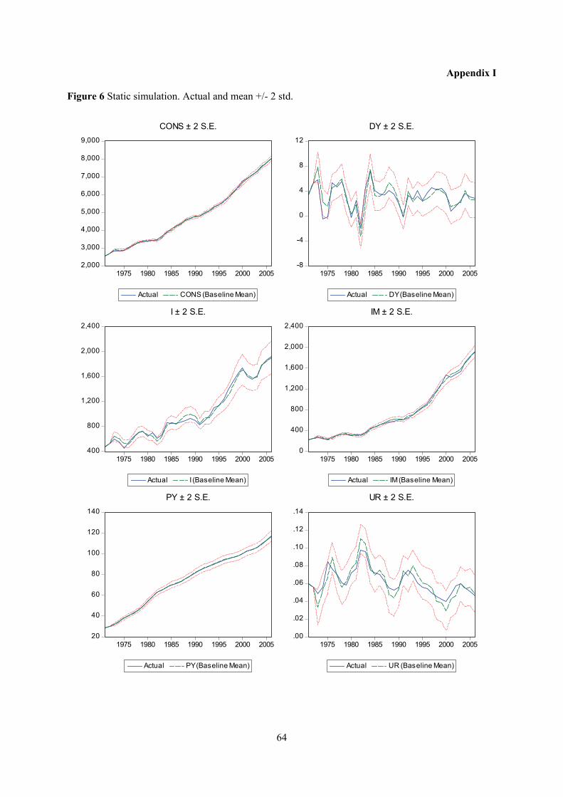
Figures 6 a-l in appendix I show that as a one-step ahead predictor, the model performs quite well for

all variables, although the ability of the model to predict investment and the unemployment rate seems

to be somewhat poorer than for the other variables. Error bounds around the predicted values of

investment and unemployment are relatively wide, reflecting greater uncertainty. Remember that Y is

not modeled directly, but is determined as the sum of four endogenous variables (CONS, EX, IM and

I) and two exogenous variables (G and STAT), and seems to fit history quite well.

An alternative way of evaluating the model is to examine how the model performs when used to

forecast many periods into “the future”. In this case, forecasts from previous periods - and not actual

historical data – are used when assigning values to the lagged endogenous terms in the model. The

22

results now illustrate model performance if we in 1970 had used the model to forecast the next 36

years, assuming we had known the correct paths for the exogenous variables. Not surprisingly, the

results displayed in Figures 7 a-l in appendix J now show more substantial deviations from actual

outcomes and error bounds are wider. Fit still seems good for most variables.

The model performs well for household consumption (CONS). Investment (I) and imports (IM) seem

to lose track somewhat in the late 1980s and early 1990s, and both are outside error bounds for a short

period, but are back on track the last ten years of the estimation period. For exports (EX) however, fit

to deteriorate from the late 1990s. The deflators for GDP and consumption shows relatively good fit,

although PY is slightly underestimated for most of the 1980s and 1990s. Modelling of the labour

market provides relatively good fit for labour supply (L). Fit for wage (WF) and particularly

employment (E) is less good. Error bounds for the unemployment rate (UR) are wide and include 0

towards the end of the period, implying a possibility greater than zero for the nonsense outcome of a

negative unemployment rate.

7. Changing the oil price An efficient way to describe important properties of the model is by simulating the model with

different assumptions for exogenous variables. This section illustrates the isolated effect of a change in

the oil price (POIL) on the US economy. Isolated, because we keep all other exogenous variables – as

interest rates, international demand and world prices – unchanged, some of which normally could have

been expected to respond to a change in the oil price.

When the model is simulated using historical residuals, it reproduces the actual historical development

of the data. Thus, when the residuals are set to their historical values in the alternative scenario with a

higher oil price, it ensures that the difference between the actual and the alternative scenario reflects

only the effect of the change in the oil price, and not model errors.

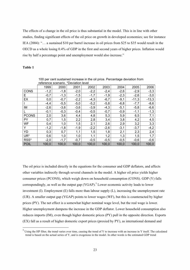
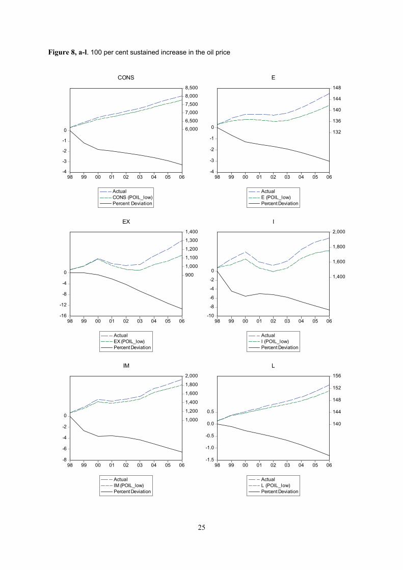
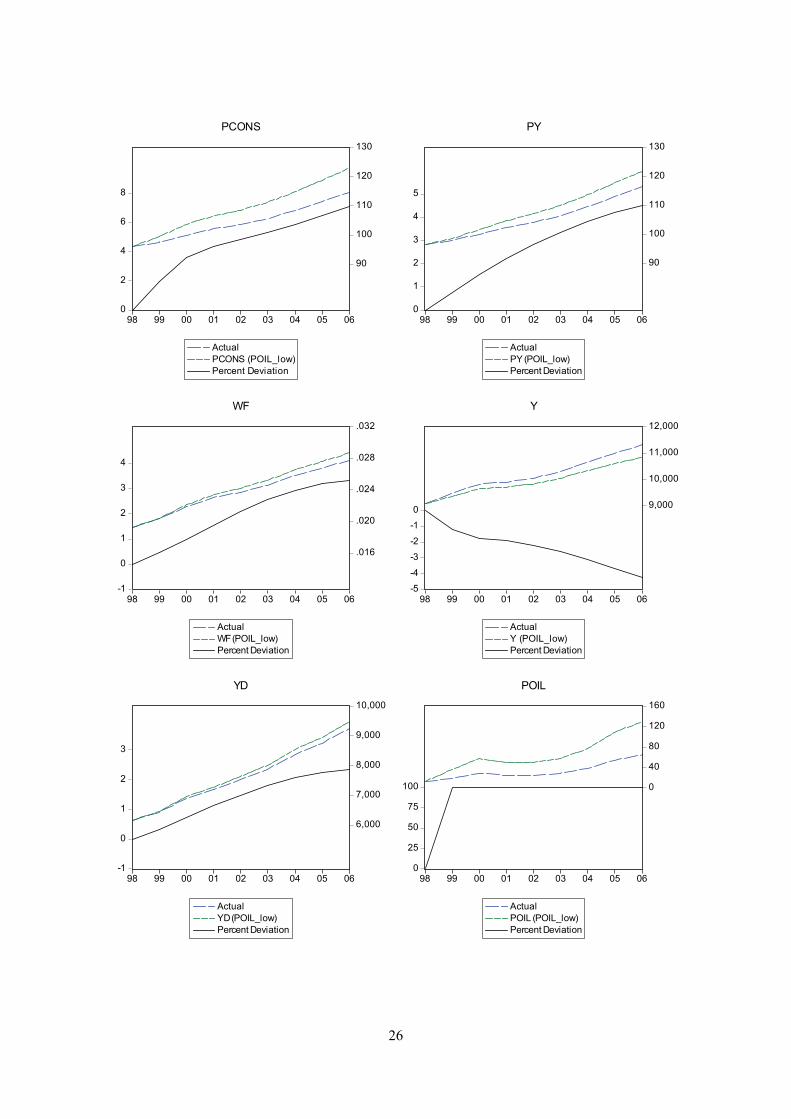
A 100 per cent sustained increase in the nominal oil price is simulated in the model; see Table 2 below

and Figures 8 a-n. Inflation picks up immediately, and after eight years consumer prices are 7.1 per

cent higher and the GDP deflator 4.5 per cent higher than in the reference scenario. Household

consumption is down by 3.3 per cent and GDP is 4.2 percentage points lower. Exports and imports fall

significantly more: this follows from high income elasticities, which is in line with what is commonly

found in studies of trade elasticities (see for instance Marquez 2002). Employment is reduced by 3.0

per cent, while the labour force only falls by 1.3 percent. The unemployment rate thus increases, by

1.7 percentage points.

23

The effects of a change in the oil price is thus substantial in the model. This is in line with other

studies, finding significant effects of the oil price on growth in developed economies; see for instance

IEA (2004): “… a sustained $10 per barrel increase in oil prices from $25 to $35 would result in the

OECD as a whole losing 0.4% of GDP in the first and second years of higher prices. Inflation would

rise by half a percentage point and unemployment would also increase.”

Table 1

100 per cent sustained increase in the oil price. Percentage deviation from reference scenario. *Deviation level

1999 2000 2001 2002 2003 2004 2005 2006 CONS -1,2 -1,8 -2,0 -2,2 -2,4 -2,6 -2,9 -3,3 E -0,7 -1,3 -1,5 -1,7 -1,9 -2,3 -2,6 -3,0 EX 0,0 -0,7 -2,2 -4,3 -6,7 -9,1 -11,3 -13,3 I -4,4 -5,5 -5,0 -5,2 -5,8 -6,8 -7,7 -8,6 IM -2,6 -3,6 -3,6 -3,9 -4,3 -5,1 -5,8 -6,6 L -0,1 -0,3 -0,4 -0,5 -0,7 -0,9 -1,1 -1,3 PCONS 2,0 3,6 4,4 4,8 5,3 5,9 6,5 7,1 PY 0,7 1,5 2,2 2,8 3,4 3,8 4,2 4,5 WF 0,4 1,0 1,5 2,1 2,6 2,9 3,2 3,3 Y -1,2 -1,8 -1,9 -2,2 -2,6 -3,1 -3,7 -4,2 YD 0,3 0,7 1,1 1,5 1,8 2,1 2,3 2,4 UR* 0,6 1,0 1,0 1,1 1,2 1,3 1,5 1,7 RSS* -2,0 -1,7 -0,7 -0,5 -0,5 -0,5 -0,6 -0,6 POIL 100,0 100,0 100,0 100,0 100,0 100,0 100,0 100,0

The oil price is included directly in the equations for the consumer and GDP deflators, and affects

other variables indirectly through several channels in the model. A higher oil price yields higher

consumer prices (PCONS), which weigh down on household consumption (CONS). GDP (Y) falls

correspondingly, as well as the output gap (YGAP).5 Lower economic activity leads to lower

investment (I). Employment (E) falls more than labour supply (L), increasing the unemployment rate

(UR). A smaller output gap (YGAP) points to lower wages (WF), but this is counteracted by higher

prices (PY). The net effect is a somewhat higher nominal wage level, but the real wage is lower.

Higher unemployment dampens the increase in the GDP deflator. Lower household consumption also

reduces imports (IM), even though higher domestic prices (PY) pull in the opposite direction. Exports

(EX) fall as a result of higher domestic export prices (proxied by PY), as international demand and

5 Using the HP filter, the trend varies over time, causing the trend of Y to increase with an increase in Y itself. The calculated

trend is based on the actual series of Y, and is exogenous in the model. In other words is the estimated GDP trend

24

international prices keep their historical values in the alternative scenario. Exports falls more than

imports and the trade balance deficit is 7.5 per cent higher after eight years. Outside the model, a

higher oil price could be expected to produce lower international prices and lower international

demand. These effects pull in opposite directions on US exports, leaving the net effect for empirical

investigation. Furthermore, higher international prices could also be expected to reduce imports. See

appendix H for other alternative scenarios, including exogenous shifts in the interest rate (RS), public

spending and investment (G), foreign demand (YG7) and foreign prices (PG7).

unaffected by the new GDP trajectory in the alternative scenario, and lower GDP thereby produces a smaller output gap (YGAP).

25

Figure 8, a-l. 100 per cent sustained increase in the oil price

-4

-3

-2

-1

0 6,000

6,500

7,000

7,500

8,000

8,500

98 99 00 01 02 03 04 05 06

ActualCONS (POIL_low)Percent Deviation

CONS

-4

-3

-2

-1

0132

136

140

144

148

98 99 00 01 02 03 04 05 06

ActualE (POIL_low)Percent Deviation

E

-16

-12

-8

-4

0 900

1,000

1,100

1,200

1,300

1,400

98 99 00 01 02 03 04 05 06

ActualEX (POIL_low)Percent Deviation

EX

-10

-8

-6

-4

-2

01,400

1,600

1,800

2,000

98 99 00 01 02 03 04 05 06

ActualI (POIL_low)Percent Deviation

I

-8

-6

-4

-2

01,000

1,200

1,400

1,600

1,800

2,000

98 99 00 01 02 03 04 05 06

ActualIM (POIL_low)Percent Deviation

IM

-1.5

-1.0

-0.5

0.0

0.5

140

144

148

152

156

98 99 00 01 02 03 04 05 06

ActualL (POIL_low)Percent Deviation

L

26

0

2

4

6

8

90

100

110

120

130

98 99 00 01 02 03 04 05 06

ActualPCONS (POIL_low)Percent Deviation

PCONS

0

1

2

3

4

5

90

100

110

120

130

98 99 00 01 02 03 04 05 06

ActualPY (POIL_low)Percent Deviation

PY

-1

0

1

2

3

4

.016

.020

.024

.028

.032

98 99 00 01 02 03 04 05 06

ActualWF (POIL_low)Percent Deviation

WF

-5

-4

-3

-2

-1

0 9,000

10,000

11,000

12,000

98 99 00 01 02 03 04 05 06

ActualY (POIL_low)Percent Deviation

Y

-1

0

1

2

3

6,000

7,000

8,000

9,000

10,000

98 99 00 01 02 03 04 05 06

ActualYD (POIL_low)Percent Deviation

YD

0

25

50

75

100 0

40

80

120

160

98 99 00 01 02 03 04 05 06

ActualPOIL (POIL_low)Percent Deviation

POIL

27

-.005

.000

.005

.010

.015

.020

.03

.04

.05

.06

.07

.08

98 99 00 01 02 03 04 05 06

ActualUR (POIL_low)Deviation

UR

-2.5

-2.0

-1.5

-1.0

-0.5

0.0-2

0

2

4

98 99 00 01 02 03 04 05 06

real interest ratereal interest rate (POIL_low)Deviation

real interest rate

28

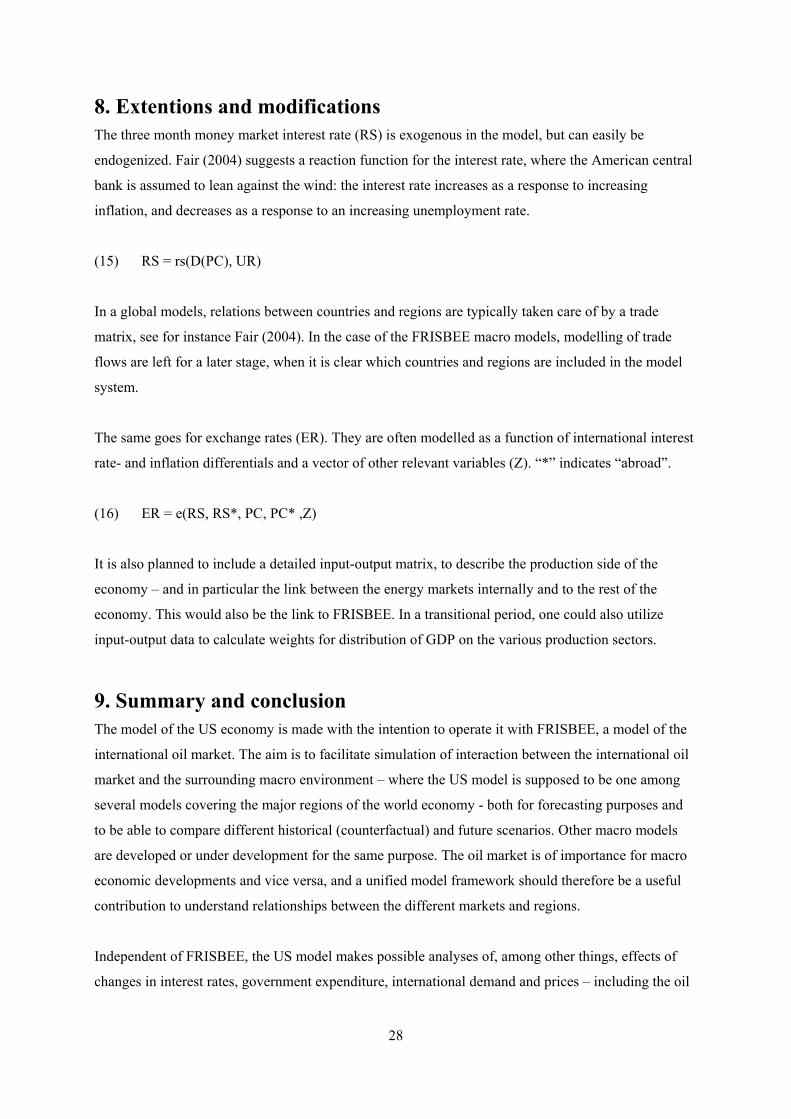
8. Extentions and modifications The three month money market interest rate (RS) is exogenous in the model, but can easily be

endogenized. Fair (2004) suggests a reaction function for the interest rate, where the American central

bank is assumed to lean against the wind: the interest rate increases as a response to increasing

inflation, and decreases as a response to an increasing unemployment rate.

(15) RS = rs(D(PC), UR)

In a global models, relations between countries and regions are typically taken care of by a trade

matrix, see for instance Fair (2004). In the case of the FRISBEE macro models, modelling of trade

flows are left for a later stage, when it is clear which countries and regions are included in the model

system.

The same goes for exchange rates (ER). They are often modelled as a function of international interest

rate- and inflation differentials and a vector of other relevant variables (Z). “*” indicates “abroad”.

(16) ER = e(RS, RS*, PC, PC* ,Z)

It is also planned to include a detailed input-output matrix, to describe the production side of the

economy – and in particular the link between the energy markets internally and to the rest of the

economy. This would also be the link to FRISBEE. In a transitional period, one could also utilize

input-output data to calculate weights for distribution of GDP on the various production sectors.

9. Summary and conclusion The model of the US economy is made with the intention to operate it with FRISBEE, a model of the

international oil market. The aim is to facilitate simulation of interaction between the international oil

market and the surrounding macro environment – where the US model is supposed to be one among

several models covering the major regions of the world economy - both for forecasting purposes and

to be able to compare different historical (counterfactual) and future scenarios. Other macro models

are developed or under development for the same purpose. The oil market is of importance for macro

economic developments and vice versa, and a unified model framework should therefore be a useful

contribution to understand relationships between the different markets and regions.

Independent of FRISBEE, the US model makes possible analyses of, among other things, effects of

changes in interest rates, government expenditure, international demand and prices – including the oil

29

price – on the US economy. The model can also be used for forecasting purposes. The estimated

equations satisfy standard statistical tests of residual properties and parameter stability. The model is

evaluated by simulating the model and comparing with historical data. Most variables are explained

fairly well by the model. However, exports and the unemployment rate fit historical data relatively

poorly, and therefore cause some concern.

An alternative scenario shows that a change in the oil price has significant effects in the model. The oil

price is increased by 10 per cent on a permanent basis. This leads to markedly higher inflation, lower

household consumption and GDP, and higher unemployment.

30

Refrences Armington, P. S. (1969): “A theory of demand for products distinguished by place of production”,

IMF Staff papers 16, No. 1, 159-176

Aune, F. R., S Glomsrød, L. Lindholt and K. E. Rosendal (2005): “Are high oil prices profitable for

OPEC in the long run?” Discussion Papers 416, Statistics Norway

Barrell, R., K. Dury and D. Holland (2001): “Macro-models and the medium term -

The NIESR experience with NiGEM”, National Institute of Economic and Social Research,

Preliminary, http://ecomod.net/conferences/ecomod2001/papers_web/Barrell_Bruss4.PDF

Bernanke, B. S., M. Gertler and M. Watson (1997): „Systematic monetary policy and the effect of oil

price shocks”. Brooking papers on economic activity 1:91:157

Boug, P., Y. Dyvi, P. R. Johansen and B. E. Naug (2002): ”MODAG – En makroøkonomisk model for

norsk økonomi (MODAG – A macro economic modell for the Norwegian economy)”, Social and

Economic Studies 108, Statistics Norway

Davidson, J. E. H.,D. F. Hendry, F. Srba and Yeo (1978): ” Econommetric modellingo f the aggregate

time series relationships between consumers’ expenditure and income inthe United Kingdom”,

Econonomic Journal 88, 661-692

Fair, R. C. (2004): “Estimating how the macro economy works”, Harvard University Press

Glomsrød, S. (2007): “A model of the Chinese economy”, Unpublished memo

Granger, C. W. J. and Y. Jeon (2007): “Evaluation of global models”, Economic Modelling

24, 980-989.

Hendry, D.F. and J.A. Doornik (2001): Modelling Dynamic Systems using PcGive Volume II,

Timberlake Consultants LTD, London.

31

Hodrick, R.J. and E.C. Prescott (1997) “Postwar U.S. Business Cycles: An Empirical Investigation”,

Journal of Money, Credit, and Banking, Vol 29, 1–16. Previously published as a working paper, but

with varying references in the literature (Working Paper or Discussion Paper nr. 451 from Carnegie-

Mellon University or Northwestern University, published in 1980 or 1981).

IEA (2004): “Analysis of high oil prices on the global economy”,

http://www.iea.org/textbase/papers/2004/high_oil_prices.pdf.

Johansen, P. R. and K. A. Magnussen(1996): “The implementation model: a macroeconomic model

for Saudi Arabia”, Documents, Statistics Norway.

Johansen, S. (1988): Statistical Analysis of Cointegration Vectors, Journal of Economic Dynamics and

Control 12, 231-254.

Korvald, H. M. (2006): “Økonomiske konsekvenser av økt oljepris for euroområdet: En empirisk

undersøkelse”, Department of Economics, University of Oslo.

Kydland, F. E. og E. C. Prescott (1990): “Business Cycles: real facts and a monetary myth”, Federal

Reserve Bank of Minneapolis, Quarterly Review (Spring).

Nymoen (2008): “Forecasts for the Norwegian economy 2008q1-2011q4”,

http://folk.uio.no/rnymoen/namforecast_mar08.pdf (see also

http://folk.uio.no/rnymoen/NAM/index.html).

Marquez, J. (2002): “Estimating Trade Elasticities”, Kluwer Academic Publishers.

Ravn, M. O. and H. Uhlig (2001): “On Adjusting the HP-filter for the Frequency of Observations”,

C.E.P.R. Discussion Papers 2858.

32

Appendix A

Data definitions and sources

National accounts data are from Bureau of economic Analyses (BEA).6 Labour market data and data

for interest rates, household wealth and household income are from Bureau of Labor Statistics (BLS)

and the Fair model data base (Fair).7 The oil price and data for the G7 countries are from OECD

Economic Outlook and OECD Main Economic Indicators.8

Variable Explanation Source

AA Total net wealth of the household sector, real Fair

CONS Household consumption expenditure BEA

Dt Impulse dummy variable for year t

E Employment, non farm total (ew:usa09216) BLS

EX Exports BEA

G Government consumption expenditures and gross investment BEA

H Hours of labour input Fair

I Gross private domestic investment BEA

IM Imports BEA

JF Number of jobs, f, millions Fair

JM Number of military jobs, millions. BLS

L Labour force BLS

PCONS Consumer prices BEA

PEX Export prices BEA

PIM Import prices BEA

POIL Oil price OECD Economic Outlook

POP Non institutional population 16 and over, millions (ew:usa50025) BLS

PY GDP deflator BEA

PYG7 GDP deflator G7 OECD Economic Outlook

RB Bond Rate Fair

RS Short interest rate Fair

STAT Statistical discrepancy BEA

T Trend

6 http://www.bea.gov/national/nipaweb/SelectTable.asp?Popular=Y , table 1.1.6 7 http://fairmodel.econ.yale.edu/usdown.htm . Download “The US model in EViews”, the database is included. Labour

market data can also be downloaded directly from the primary source, Bureau of Labor Statistics: http://www.bls.gov 8 G7GDP (MEI) = G7M.CMPGDP.VIXOBSA.A G7GDP-deflator (Economic Outlook)=Y.BIG7.PGDP

33

ULC Unit labour cost BLS

UR Unemployment rate BLS

WF Average wage per hour excluding overtime, private sector BLS

X Household disposable income less private sector wage income Equation 17

Y Real GDP BEA

YD Disposable income of the household sector, nominal Fair

YG7 Real GDP G7 OECD MEI

YGAP Output gap Benedictow

YHP GDP trend (HP, Lambda 100)9 Benedictow

9 For the purpose of HP- filtering, the GDP series was extended with forecasts to 2009 from

http://fairmodel.econ.yale.edu/usdown.htm

34

Appendix B

Testing normal distribution of residuals

0

1

2

3

4

5

6

7

8

-0.01 0.00 0.01

Series: ResidualsSample 1955 2006Observations 52

Mean -1.11e-16Median 0.000419Maximum 0.015514Minimum -0.016564Std. Dev. 0.007961Skewness -0.111548Kurtosis 2.220870

Jarque-Bera 1.423101Probability 0.490883

CONS

0

2

4

6

8

10

-0.10 -0.05 -0.00 0.05




I

35

0

1

2

3

4

5

6

7

8

-0.06 -0.04 -0.02 0.00 0.02 0.04 0.06


Mean -1.02e-15Median 0.000382Maximum 0.066243Minimum -0.054964Std. Dev. 0.026113Skewness 0.138369Kurtosis 3.190345


EX

0

1

2

3

4

5

6

7

8

-0.06 -0.04 -0.02 0.00 0.02 0.04 0.06


Mean 2.22e-16Median 0.000628Maximum 0.061638Minimum -0.059074Std. Dev. 0.026281Skewness 0.087340Kurtosis 2.482545


IM

36

0

1

2

3

4

5

6

7

-0.005 0.000 0.005


Mean 4.20e-17Median -8.98e-05Maximum 0.007390Minimum -0.006755Std. Dev. 0.003489Skewness 0.118949Kurtosis 2.301500


PY

0

1

2

3

4

5

6

7

8

9

-0.005 0.000 0.005




PCONS

37

0

1

2

3

4

5

6

7

8

9

-0.010 -0.005 0.000 0.005 0.010 0.015




E

0

1

2

3

4

5

6

7

8

-0.02 -0.01 -0.00 0.01 0.02




WF

38

0

2

4

6

8

10

-0.005 0.000 0.005




L

39

Appendix C

Testing for first order heteroscedatsticity in the residuals. The ARCH test for heteroskedasticity in the residual regresses the squared residuals on lagged squared residuals and a constant. In the presence of heteroskedasticity, ordinary least squares estimates are still consistent, but the conventional computed standard errors are no longer valid. CONS Heteroskedasticity Test: ARCH

F-statistic 0.005633 Prob. F(1,49) 0.9405Obs*R-squared 0.005862 Prob. Chi-Square(1) 0.9390

I Heteroskedasticity Test: ARCH


EX Heteroskedasticity Test: ARCH


IM Heteroskedasticity Test: ARCH


PY Heteroskedasticity Test: ARCH


PCONS Heteroskedasticity Test: ARCH


40

E Heteroskedasticity Test: ARCH


WF Heteroskedasticity Test: ARCH


L Heteroskedasticity Test: ARCH


41

Appendix D

Serial correlation CONS Breusch-Godfrey Serial Correlation LM Test:

F-statistic 0.174210 Prob. F(4,43) 0.9504 Obs*R-squared 0.829251 Prob. Chi-Square(4) 0.9345

I Breusch-Godfrey Serial Correlation LM Test:


EX Breusch-Godfrey Serial Correlation LM Test:


IM Breusch-Godfrey Serial Correlation LM Test:


PY Breusch-Godfrey Serial Correlation LM Test:


PCONS Breusch-Godfrey Serial Correlation LM Test:


E Breusch-Godfrey Serial Correlation LM Test:


42

WF Breusch-Godfrey Serial Correlation LM Test:


L Breusch-Godfrey Serial Correlation LM Test:


43

Appendix E

Recursive coefficients CONS

-1

0

1

2

3

4

5

65 70 75 80 85 90 95 00 05

Recursive C(1) Estimates± 2 S.E.

-.6

-.4

-.2

.0

.2

.4

.6

65 70 75 80 85 90 95 00 05


0.2

0.4

0.6

0.8

1.0

1.2

1.4

1.6

65 70 75 80 85 90 95 00 05


-.3

-.2

-.1

.0

.1

.2

.3

.4

65 70 75 80 85 90 95 00 05


-1.6

-1.2

-0.8

-0.4

0.0

0.4

65 70 75 80 85 90 95 00 05


44

I

-3

-2

-1

0

1

70 75 80 85 90 95 00 05


-1.0

-0.8

-0.6

-0.4

-0.2

0.0

0.2

70 75 80 85 90 95 00 05


-.015

-.010

-.005

.000

.005

.010

.015

70 75 80 85 90 95 00 05


2.0

2.5

3.0

3.5

4.0

4.5

70 75 80 85 90 95 00 05


45

EX

-10

-8

-6

-4

-2

0

1985 1990 1995 2000 2005


-1.2

-0.8

-0.4

0.0

0.4

0.8

1985 1990 1995 2000 2005


-3

-2

-1

0

1

2

1985 1990 1995 2000 2005


-3

-2

-1

0

1

2

1985 1990 1995 2000 2005


0

1

2

3

4

1985 1990 1995 2000 2005


-.8

-.4

.0

.4

.8

1985 1990 1995 2000 2005


0

1

2

3

4

5

1985 1990 1995 2000 2005


46

IM

-10

-8

-6

-4

-2

0

2

4

70 75 80 85 90 95 00 05


-1.2

-0.8

-0.4

0.0

0.4

0.8

70 75 80 85 90 95 00 05


-1.0

-0.5

0.0

0.5

1.0

1.5

2.0

70 75 80 85 90 95 00 05


-3

-2

-1

0

1

2

70 75 80 85 90 95 00 05


-1.0

-0.5

0.0

0.5

1.0

1.5

2.0

2.5

70 75 80 85 90 95 00 05


.00

.01

.02

.03

.04

70 75 80 85 90 95 00 05


47

PY

-.2

-.1

.0

.1

.2

.3

.4

1985 1990 1995 2000 2005

Recursiv e C(1) Estimates± 2 S.E.

-.25

-.20

-.15

-.10

-.05

.00

1985 1990 1995 2000 2005


.00

.05

.10

.15

.20

.25

1985 1990 1995 2000 2005


-.8

-.6

-.4

-.2

.0

1985 1990 1995 2000 2005


-.06

-.04

-.02

.00

.02

.04

1985 1990 1995 2000 2005


-.6

-.4

-.2

.0

.2

.4

1985 1990 1995 2000 2005


.00

.04

.08

.12

.16

.20

1985 1990 1995 2000 2005


-.03

-.02

-.01

.00

.01

.02

.03

1985 1990 1995 2000 2005


.00

.02

.04

.06

.08

.10

1985 1990 1995 2000 2005


48

PCONS

-.5

-.4

-.3

-.2

-.1

.0

.1

1975 1980 1985 1990 1995 2000 2005


-.4

-.3

-.2

-.1

.0

.1

.2

.3

1975 1980 1985 1990 1995 2000 2005


-.2

-.1

.0

.1

.2

.3

.4

1975 1980 1985 1990 1995 2000 2005


.00

.01

.02

.03

.04

1975 1980 1985 1990 1995 2000 2005


-.06

-.04

-.02

.00

.02

.04

1975 1980 1985 1990 1995 2000 2005


.2

.3

.4

.5

.6

.7

1975 1980 1985 1990 1995 2000 2005


-.8

-.6

-.4

-.2

.0

.2

.4

.6

1975 1980 1985 1990 1995 2000 2005


49

E

-1

0

1

2

3

65 70 75 80 85 90 95 00 05


-1.6

-1.2

-0.8

-0.4

0.0

0.4

65 70 75 80 85 90 95 00 05


-.2

-.1

.0

.1

.2

.3

.4

.5

65 70 75 80 85 90 95 00 05


-0.2

0.0

0.2

0.4

0.6

0.8

1.0

65 70 75 80 85 90 95 00 05


.002

.003

.004

.005

.006

.007

.008

.009

65 70 75 80 85 90 95 00 05


50

WF

-15

-10

-5

0

5

10

70 75 80 85 90 95 00 05


-1.2

-0.8

-0.4

0.0

0.4

0.8

70 75 80 85 90 95 00 05


-1.0

-0.5

0.0

0.5

1.0

1.5

70 75 80 85 90 95 00 05


-.4

-.2

.0

.2

.4

.6

.8

70 75 80 85 90 95 00 05


-0.5

0.0

0.5

1.0

1.5

2.0

2.5

70 75 80 85 90 95 00 05


-1.2

-0.8

-0.4

0.0

0.4

0.8

70 75 80 85 90 95 00 05


51

L

-6

-4

-2

0

2

4

6

70 75 80 85 90 95 00 05


-1.0

-0.8

-0.6

-0.4

-0.2

0.0

0.2

0.4

70 75 80 85 90 95 00 05


-.3

-.2

-.1

.0

.1

.2

70 75 80 85 90 95 00 05


-.1

.0

.1

.2

.3

.4

70 75 80 85 90 95 00 05


-.6

-.4

-.2

.0

.2

.4

70 75 80 85 90 95 00 05


-2

-1

0

1

2

3

70 75 80 85 90 95 00 05


-.3

-.2

-.1

.0

.1

.2

.3

70 75 80 85 90 95 00 05


52

Appendix F

Recursive residuals CONS

-.020

-.015

-.010

-.005

.000

.005

.010

.015

.020

60 65 70 75 80 85 90 95 00 05

Recursive Residuals ± 2 S.E.

I

-.06

-.04

-.02

.00

.02

.04

.06

1965 1970 1975 1980 1985 1990 1995 2000 2005


53

EX

-.08

-.06

-.04

-.02

.00

.02

.04

.06

.08

1980 1985 1990 1995 2000 2005


IM

-.100

-.075

-.050

-.025

.000

.025

.050

.075

.100

1970 1975 1980 1985 1990 1995 2000 2005


54

PY

-.0100

-.0075

-.0050

-.0025

.0000

.0025

.0050

.0075

.0100

1980 1985 1990 1995 2000 2005


PCONS

-.012

-.008

-.004

.000

.004

.008

.012

.016

1970 1975 1980 1985 1990 1995 2000 2005


55

E

-.020

-.015

-.010

-.005

.000

.005

.010

.015

.020

60 65 70 75 80 85 90 95 00 05


WF

-.04

-.03

-.02

-.01

.00

.01

.02

.03

1965 1970 1975 1980 1985 1990 1995 2000 2005


56

L

-.016

-.012

-.008

-.004

.000

.004

.008

.012

.016

65 70 75 80 85 90 95 00 05


57

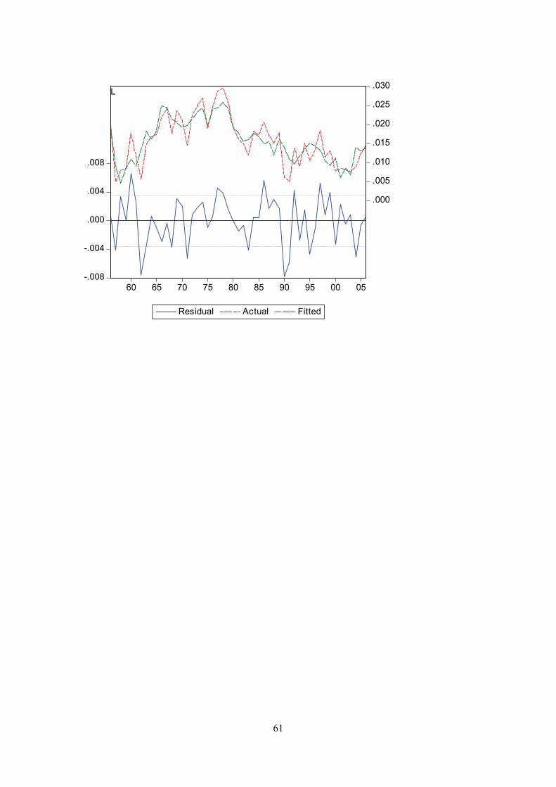
Appendix G

Actual and fitted values of the dependent variable and the residuals from the regression. I.e. the first graph displays actual and fitted d(log(cons/pop)), and the equation residual.

-.02

-.01

.00

.01

.02

-.02

.00

.02

.04

.06

.08

55 60 65 70 75 80 85 90 95 00 05

Residual Actual Fitted

CONS

-.12

-.08

-.04

.00

.04

.08 -.2

-.1

.0

.1

.2

.3

60 65 70 75 80 85 90 95 00 05


I

58

-.08

-.04

.00

.04

.08

-.10

-.05

.00

.05

.10

.15

.20

1975 1980 1985 1990 1995 2000 2005


EX

-.08

-.04

.00

.04

.08

-.2

-.1

.0

.1

.2

.3

60 65 70 75 80 85 90 95 00 05


IM

59

-.008

-.004

.000

.004

.008

.00

.02

.04

.06

.08

.10

1970 1975 1980 1985 1990 1995 2000 2005


PY

-.012

-.008

-.004

.000

.004

.008

.00

.02

.04

.06

.08

.10

.12

65 70 75 80 85 90 95 00 05


PCONS

60

-.015

-.010

-.005

.000

.005

.010

.015

-.04

-.02

.00

.02

.04

.06

55 60 65 70 75 80 85 90 95 00 05


E

-.03

-.02

-.01

.00

.01

.02

.03.00

.02

.04

.06

.08

.10

.12

60 65 70 75 80 85 90 95 00 05


WF

61

-.008

-.004

.000

.004

.008

.000

.005

.010

.015

.020

.025

.030

60 65 70 75 80 85 90 95 00 05


L

62

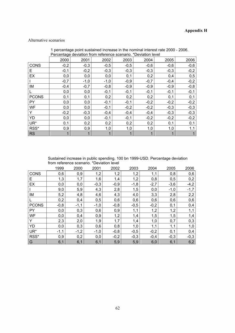
Appendix H

Alternative scenarios

1 percentage point sustained increase in the nominal interest rate 2000 - 2006. Percentage deviation from reference scenario. *Deviation level

2000 2001 2002 2003 2004 2005 2006CONS -0,2 -0,3 -0,5 -0,5 -0,6 -0,6 -0,6E -0,1 -0,2 -0,3 -0,3 -0,3 -0,3 -0,2EX 0,0 0,0 0,0 0,1 0,2 0,4 0,5I -0,7 -1,0 -1,0 -0,9 -0,7 -0,4 -0,2IM -0,4 -0,7 -0,8 -0,9 -0,9 -0,9 -0,8L 0,0 0,0 -0,1 -0,1 -0,1 -0,1 -0,1PCONS 0,1 0,1 0,2 0,2 0,2 0,1 0,1PY 0,0 0,0 -0,1 -0,1 -0,2 -0,2 -0,2WF 0,0 0,0 -0,1 -0,2 -0,2 -0,3 -0,3Y -0,2 -0,3 -0,4 -0,4 -0,4 -0,3 -0,3YD 0,0 0,0 -0,1 -0,1 -0,2 -0,2 -0,2UR* 0,1 0,2 0,2 0,2 0,2 0,1 0,1RSS* 0,9 0,9 1,0 1,0 1,0 1,0 1,1RS 1 1 1 1 1 1 1

Sustained increase in public spending, 100 bn 1999-USD. Percentage deviation from reference scenario. *Deviation level

1999 2000 2001 2002 2003 2004 2005 2006 CONS 0,6 0,9 1,2 1,2 1,2 1,1 0,8 0,6 E 1,3 1,7 1,6 1,4 1,2 0,8 0,5 0,2 EX 0,0 0,0 -0,3 -0,9 -1,8 -2,7 -3,6 -4,2 I 9,0 5,9 4,3 2,8 1,5 0,0 -1,0 -1,7 IM 5,2 4,8 4,6 4,3 4,0 3,3 2,8 2,2 L 0,2 0,4 0,5 0,6 0,6 0,6 0,6 0,6 PCONS -0,8 -1,1 -1,0 -0,8 -0,5 -0,2 0,1 0,4 PY 0,0 0,3 0,6 0,9 1,1 1,2 1,2 1,1 WF 0,0 0,4 0,9 1,2 1,4 1,5 1,5 1,4 Y 2,3 2,0 1,9 1,7 1,4 1,0 0,7 0,3 YD 0,0 0,3 0,6 0,8 1,0 1,1 1,1 1,0 UR* -1,1 -1,2 -1,0 -0,8 -0,5 -0,2 0,1 0,4 RSS* 0,9 0,2 0,0 -0,2 -0,3 -0,4 -0,3 -0,3 G 6,1 6,1 6,1 5,9 5,9 6,0 6,1 6,2

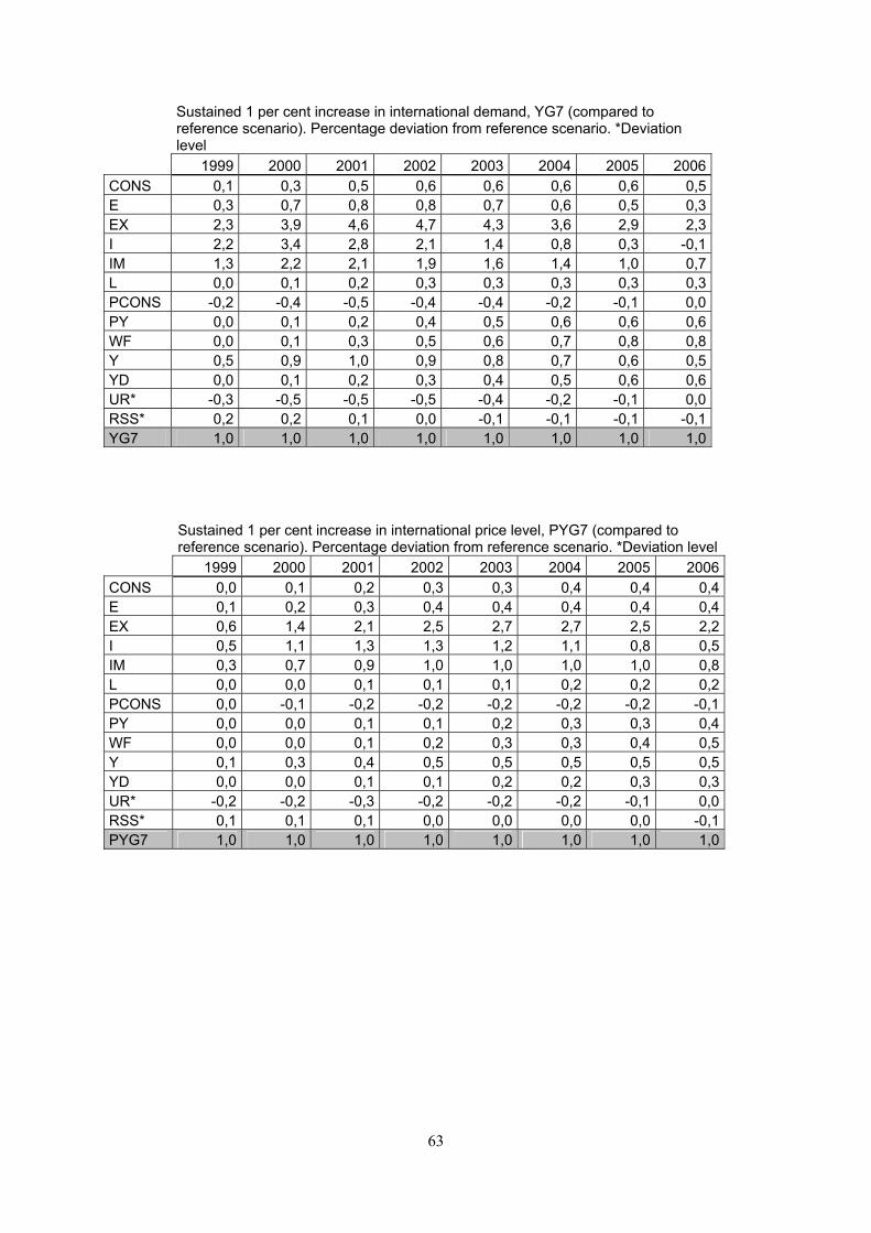
63

Sustained 1 per cent increase in international demand, YG7 (compared to reference scenario). Percentage deviation from reference scenario. *Deviation level

1999 2000 2001 2002 2003 2004 2005 2006 CONS 0,1 0,3 0,5 0,6 0,6 0,6 0,6 0,5 E 0,3 0,7 0,8 0,8 0,7 0,6 0,5 0,3 EX 2,3 3,9 4,6 4,7 4,3 3,6 2,9 2,3 I 2,2 3,4 2,8 2,1 1,4 0,8 0,3 -0,1 IM 1,3 2,2 2,1 1,9 1,6 1,4 1,0 0,7 L 0,0 0,1 0,2 0,3 0,3 0,3 0,3 0,3 PCONS -0,2 -0,4 -0,5 -0,4 -0,4 -0,2 -0,1 0,0 PY 0,0 0,1 0,2 0,4 0,5 0,6 0,6 0,6 WF 0,0 0,1 0,3 0,5 0,6 0,7 0,8 0,8 Y 0,5 0,9 1,0 0,9 0,8 0,7 0,6 0,5 YD 0,0 0,1 0,2 0,3 0,4 0,5 0,6 0,6 UR* -0,3 -0,5 -0,5 -0,5 -0,4 -0,2 -0,1 0,0 RSS* 0,2 0,2 0,1 0,0 -0,1 -0,1 -0,1 -0,1 YG7 1,0 1,0 1,0 1,0 1,0 1,0 1,0 1,0

Sustained 1 per cent increase in international price level, PYG7 (compared to reference scenario). Percentage deviation from reference scenario. *Deviation level

1999 2000 2001 2002 2003 2004 2005 2006 CONS 0,0 0,1 0,2 0,3 0,3 0,4 0,4 0,4 E 0,1 0,2 0,3 0,4 0,4 0,4 0,4 0,4 EX 0,6 1,4 2,1 2,5 2,7 2,7 2,5 2,2 I 0,5 1,1 1,3 1,3 1,2 1,1 0,8 0,5 IM 0,3 0,7 0,9 1,0 1,0 1,0 1,0 0,8 L 0,0 0,0 0,1 0,1 0,1 0,2 0,2 0,2 PCONS 0,0 -0,1 -0,2 -0,2 -0,2 -0,2 -0,2 -0,1 PY 0,0 0,0 0,1 0,1 0,2 0,3 0,3 0,4 WF 0,0 0,0 0,1 0,2 0,3 0,3 0,4 0,5 Y 0,1 0,3 0,4 0,5 0,5 0,5 0,5 0,5 YD 0,0 0,0 0,1 0,1 0,2 0,2 0,3 0,3 UR* -0,2 -0,2 -0,3 -0,2 -0,2 -0,2 -0,1 0,0 RSS* 0,1 0,1 0,1 0,0 0,0 0,0 0,0 -0,1 PYG7 1,0 1,0 1,0 1,0 1,0 1,0 1,0 1,0

64

Appendix I

Figure 6 Static simulation. Actual and mean +/- 2 std.

2,000

3,000

4,000

5,000

6,000

7,000

8,000

9,000

1975 1980 1985 1990 1995 2000 2005

Actual CONS (Baseline Mean)

CONS ± 2 S.E.

-8

-4

0

4

8

12

1975 1980 1985 1990 1995 2000 2005

Actual DY (Baseline Mean)

DY ± 2 S.E.

400

800

1,200

1,600

2,000

2,400

1975 1980 1985 1990 1995 2000 2005

Actual I (Baseline Mean)

I ± 2 S.E.

0

400

800

1,200

1,600

2,000

2,400

1975 1980 1985 1990 1995 2000 2005

Actual IM (Baseline Mean)

IM ± 2 S.E.

20

40

60

80

100

120

140

1975 1980 1985 1990 1995 2000 2005

Actual PY (Baseline Mean)

PY ± 2 S.E.

.00

.02

.04

.06

.08

.10

.12

.14

1975 1980 1985 1990 1995 2000 2005

Actual UR (Baseline Mean)

UR ± 2 S.E.

65

80

90

100

110

120

130

140

150

1975 1980 1985 1990 1995 2000 2005

Actual E (Baseline Mean)

E ± 2 S.E.

0

200

400

600

800

1,000

1,200

1,400

1975 1980 1985 1990 1995 2000 2005

Actual EX (Baseline Mean)

EX ± 2 S.E.

80

100

120

140

160

1975 1980 1985 1990 1995 2000 2005

Actual L (Baseline Mean)

L ± 2 S.E.

20

40

60

80

100

120

1975 1980 1985 1990 1995 2000 2005

Actual PCONS (Baseline Mean)

PCONS ± 2 S.E.

.000

.005

.010

.015

.020

.025

.030

1975 1980 1985 1990 1995 2000 2005

Actual WF (Baseline Mean)

WF ± 2 S.E.

2,000

4,000

6,000

8,000

10,000

12,000

1975 1980 1985 1990 1995 2000 2005

Actual Y (Baseline Mean)

Y ± 2 S.E.

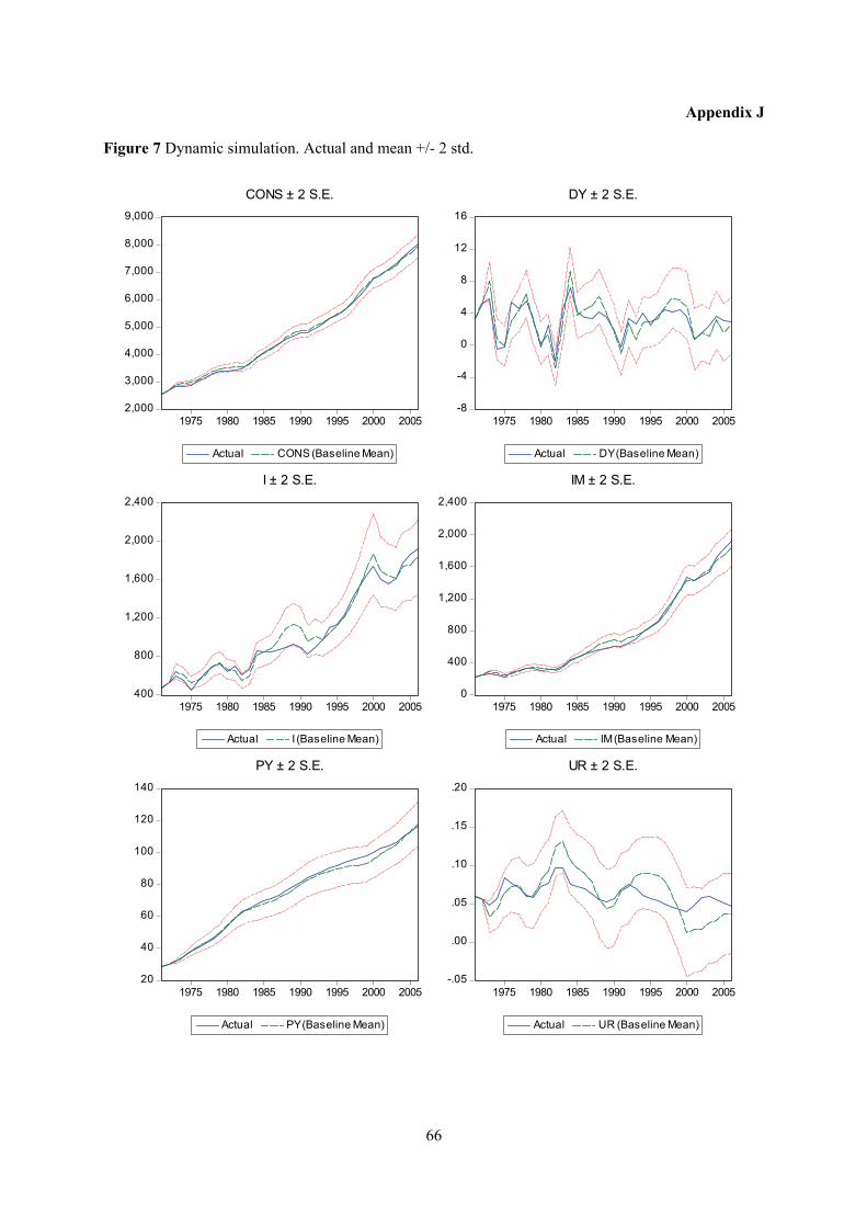
66

Appendix J

Figure 7 Dynamic simulation. Actual and mean +/- 2 std.

2,000

3,000

4,000

5,000

6,000

7,000

8,000

9,000

1975 1980 1985 1990 1995 2000 2005

Actual CONS (Baseline Mean)

CONS ± 2 S.E.

-8

-4

0

4

8

12

16

1975 1980 1985 1990 1995 2000 2005

Actual DY (Baseline Mean)

DY ± 2 S.E.

400

800

1,200

1,600

2,000

2,400

1975 1980 1985 1990 1995 2000 2005

Actual I (Baseline Mean)

I ± 2 S.E.

0

400

800

1,200

1,600

2,000

2,400

1975 1980 1985 1990 1995 2000 2005

Actual IM (Baseline Mean)

IM ± 2 S.E.

20

40

60

80

100

120

140

1975 1980 1985 1990 1995 2000 2005

Actual PY (Baseline Mean)

PY ± 2 S.E.

-.05

.00

.05

.10

.15

.20

1975 1980 1985 1990 1995 2000 2005

Actual UR (Baseline Mean)

UR ± 2 S.E.

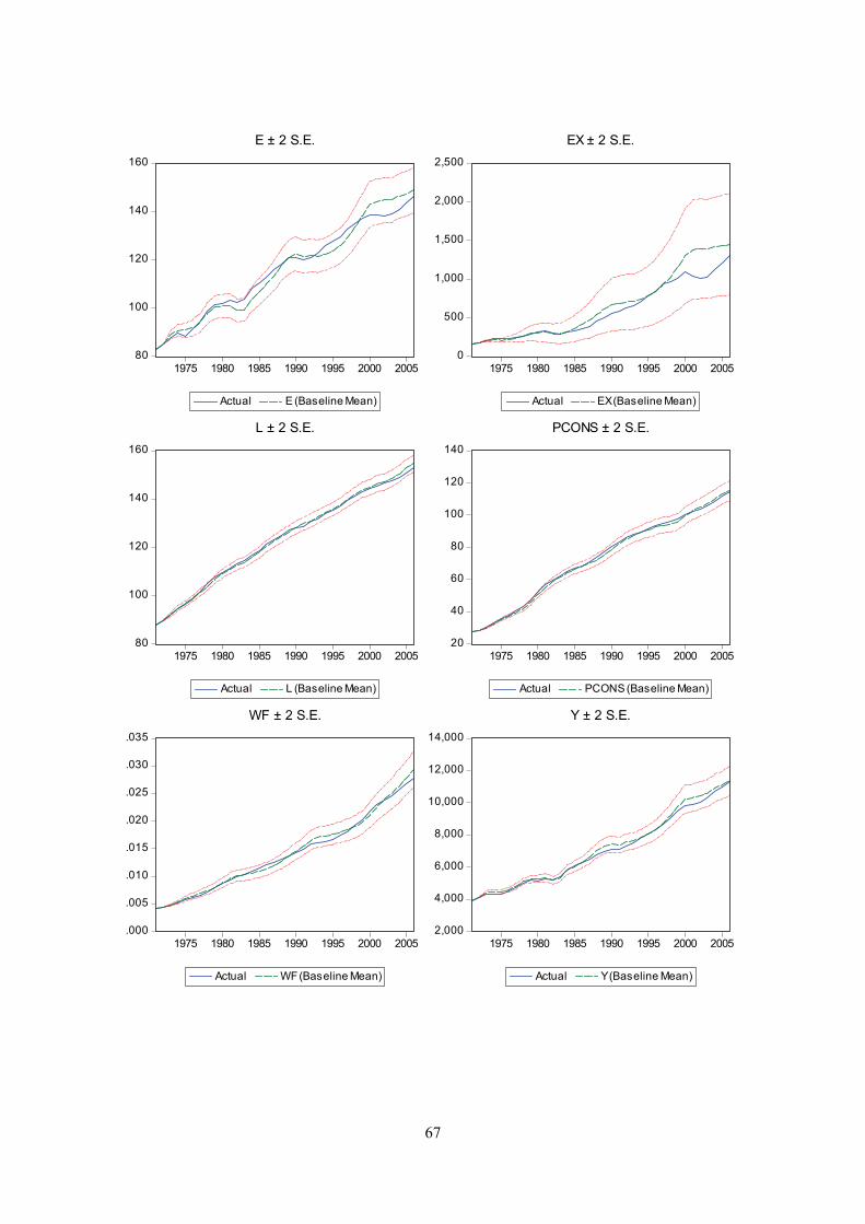
67

80

100

120

140

160

1975 1980 1985 1990 1995 2000 2005

Actual E (Baseline Mean)

E ± 2 S.E.

0

500

1,000

1,500

2,000

2,500

1975 1980 1985 1990 1995 2000 2005

Actual EX (Baseline Mean)

EX ± 2 S.E.

80

100

120

140

160

1975 1980 1985 1990 1995 2000 2005

Actual L (Baseline Mean)

L ± 2 S.E.

20

40

60

80

100

120

140

1975 1980 1985 1990 1995 2000 2005

Actual PCONS (Baseline Mean)

PCONS ± 2 S.E.

.000

.005

.010

.015

.020

.025

.030

.035

1975 1980 1985 1990 1995 2000 2005

Actual WF (Baseline Mean)

WF ± 2 S.E.

2,000

4,000

6,000

8,000

10,000

12,000

14,000

1975 1980 1985 1990 1995 2000 2005

Actual Y (Baseline Mean)

Y ± 2 S.E.

A small macro econometric model of the US economy - SSB

Documents

Transcript of A small macro econometric model of the US economy - SSB