A single-manufacturer multi-retailer integrated inventory ...
33
RAIRO-Oper. Res. 55 (2021) 3459–3491 RAIRO Operations Research https://doi.org/10.1051/ro/2021156 www.rairo-ro.org A SINGLE-MANUFACTURER MULTI-RETAILER INTEGRATED INVENTORY MODEL FOR ITEMS WITH IMPERFECT QUALITY, PRICE SENSITIVE DEMAND AND PLANNED BACK ORDERS Dipak Barman and Gour Chandra Mahata * Abstract. In this paper, we develop an integrated two-echelon supply chain inventory model with a single-manufacturer and multi-retailers in which each retailer’s demand is dependent on selling price of the product. The manufacturer produces a single product and dispatched the order quantities of the retailers in some equal batches. The production process is imperfect and produces imperfect quality of products with a defective percentage which is random in nature and follows binomial distribution. Inspection process is performed by the retailers to classify the defective items in each lot delivered from the manufacturer. The defective items that were found by the retailer will be returned to the manufacturer at the next delivery. Lead time is random and it follows an exponential distribution. We also assume that shortages are allowed and are completely backlogged at each retailer’s end. A closed form solution to maximize the expected average profit for both the centralized and the decentralized scenarios are obtained. The developed models are illustrated with the help of some numerical examples using stochastic search genetic algorithm (GA). It is found that integration of the supply chain players results an impressive increment in the profit of the whole supply chain. Sensitivity analysis is also performed to explore the impacts of key-model parameters on the expected average profit of the supply chain. Mathematics Subject Classification. 90B05. Received June 24, 2021. Accepted October 11, 2021. 1. Introduction With the growing fixate on supply chain management over the last two decenniums, firms endeavors to accomplish more preponderant collaborative advantages with their supply chain partners. Subsequently, there is a tremendous growing interest in jointly optimizing the engenderment and inventory quandaries for the supply chain partners. Integrated inventory management has recently received a great deal of attention. Nowadays, due to the globalization of the rialto and expeditiously incrementing competition between sundry opposition organizations, companies are facing sundry obstacles to compete exclusively. So, collaboration between different business units leads to a consequential way to obtain spirited advantage. For better efficiency, the supply chain players are exhibiting great interest in making their decisions jointly. Since 1976 Goyal [15] was the first author Keywords. Two-echelon supply chain, Single-manufacturer, Multi-retailers, Imperfect quality items, Price dependent demand, Stochastic lead time, Genetic algorithm. 1 Department of Mathematics, Sidho-Kanho-Birsha University, Purulia 723104, India * Corresponding author: [email protected] c ○ The authors. Published by EDP Sciences, ROADEF, SMAI 2021 This is an Open Access article distributed under the terms of the Creative Commons Attribution License (https://creativecommons.org/licenses/by/4.0), which permits unrestricted use, distribution, and reproduction in any medium, provided the original work is properly cited.
Transcript of A single-manufacturer multi-retailer integrated inventory ...

RAIRO-Oper. Res. 55 (2021) 3459–3491 RAIRO Operations Researchhttps://doi.org/10.1051/ro/2021156 www.rairo-ro.org
A SINGLE-MANUFACTURER MULTI-RETAILER INTEGRATED INVENTORYMODEL FOR ITEMS WITH IMPERFECT QUALITY, PRICE SENSITIVE
DEMAND AND PLANNED BACK ORDERS
Dipak Barman and Gour Chandra Mahata*
Abstract. In this paper, we develop an integrated two-echelon supply chain inventory model with asingle-manufacturer and multi-retailers in which each retailer’s demand is dependent on selling priceof the product. The manufacturer produces a single product and dispatched the order quantities of theretailers in some equal batches. The production process is imperfect and produces imperfect qualityof products with a defective percentage which is random in nature and follows binomial distribution.Inspection process is performed by the retailers to classify the defective items in each lot deliveredfrom the manufacturer. The defective items that were found by the retailer will be returned to themanufacturer at the next delivery. Lead time is random and it follows an exponential distribution. Wealso assume that shortages are allowed and are completely backlogged at each retailer’s end. A closedform solution to maximize the expected average profit for both the centralized and the decentralizedscenarios are obtained. The developed models are illustrated with the help of some numerical examplesusing stochastic search genetic algorithm (GA). It is found that integration of the supply chain playersresults an impressive increment in the profit of the whole supply chain. Sensitivity analysis is alsoperformed to explore the impacts of key-model parameters on the expected average profit of the supplychain.
Mathematics Subject Classification. 90B05.
Received June 24, 2021. Accepted October 11, 2021.
1. Introduction
With the growing fixate on supply chain management over the last two decenniums, firms endeavors toaccomplish more preponderant collaborative advantages with their supply chain partners. Subsequently, there isa tremendous growing interest in jointly optimizing the engenderment and inventory quandaries for the supplychain partners. Integrated inventory management has recently received a great deal of attention. Nowadays,due to the globalization of the rialto and expeditiously incrementing competition between sundry oppositionorganizations, companies are facing sundry obstacles to compete exclusively. So, collaboration between differentbusiness units leads to a consequential way to obtain spirited advantage. For better efficiency, the supply chainplayers are exhibiting great interest in making their decisions jointly. Since 1976 Goyal [15] was the first author
Keywords. Two-echelon supply chain, Single-manufacturer, Multi-retailers, Imperfect quality items, Price dependent demand,Stochastic lead time, Genetic algorithm.
1 Department of Mathematics, Sidho-Kanho-Birsha University, Purulia 723104, India*Corresponding author: [email protected]
c○ The authors. Published by EDP Sciences, ROADEF, SMAI 2021
This is an Open Access article distributed under the terms of the Creative Commons Attribution License (https://creativecommons.org/licenses/by/4.0),which permits unrestricted use, distribution, and reproduction in any medium, provided the original work is properly cited.
3460 D. BARMAN ET AL.
who introduced integration between supply chain members in inventory model with finite production rate. Later,many researchers (Banerjee [2], Ben-Daya and Hariga [7], Dey et al. [10], Jindala and Solanki [21]) presentedvarious integrated inventory models.
The supply chain management involves with the activities for coordinating the raw materials, information,production and financial flow to consummate the customer demand with the aim of maximizing customervalue and gaining competitive advantage in the market. In a supply chain, raw materials are distributed to themanufacturer from the supplier, then engendered items are transferred from the manufacturer to the retailerand conclusively distributed to the terminus customers to meet their injunctive authorization. In the presentcompetitive market, the selling price of a product is one of the most consequential factors to the retailers.Generally, higher selling price of a product abbreviates the ordinate dictation, and plausible and low sellingprice increases the authoritative ordinance of the product. Therefore, price-dependent stochastic demand isvery much a practical case in supply chain management. The most paramount factor that affects the consumerdemand is the retail price of the product. The customer demand falls with the incrimination in retail prices.So, many companies are now fixating on achieving the best pricing strategy to increment the sales volume.Many researchers like Yang et al. [50], Barman and Das [3], Ray and Jewkes [37], Kocabiyikoglu and Popescu[24], Bhowmick and Samanta [8], Mahato et al. [28], Pervin et al. [34] developed their models considering pricesensitive demand. In the classical inventory and supply chain models, the market demand is surmised to beconstant. However, in authenticity, there are many items whose demands are merely not constant but dependon the retail price. If the price is low, then the market demand is more; on the other hand, if the price is highthen the market demand of the product is less. So, the selling price plays a consequential role in determining theinventory or supply chain strategies. In this paper, we will fixate on an integrated retailer-manufacturer modelfor imperfect quality of items having price-dependent market demand. Shortages in the retailer’s inventoryare sanctioned to occur and are planned backlogged. The objective of this study is to determine the optimaldecisions which maximize the joint total profit of the whole supply chain.
In today’s business world, manufacturer uses several retailers to sell their products rather than rely on asingle retailer. The multi-buyer situation is very common in real life. A manufacturer may supply his/herproduct to different retailers to fulfil their requirements. For example, in health care industries, the manufacturersupplies instruments to different hospitals according to their requirements. They often give much accentuationon controlling distribution lead time in order to efficiently handle a supply chain. Lead time refers to the timeinterval between order placement and receiving the distribution of items. It may be desultory in nature. Itaffects the injunctive sanction forecasting and makes the customer probing for alternatives. So, for an efficientmanagement of supply chain and facilitate economic prosperity, it is essential to concentrate on such a sensiblefactor. Yang and Geunes [51] provided a nice discussion about inventory and lead time planning with lead timesensitive demand. The literary review reflects that numerous research works have been carried out focusing onlead time (Ouyang et al. [31], Gholami and Mirzazadeh [11]). In two-level supply chain system, a fascinatingstrategic quandary arises at the retailer’s end in determining optimal authoritatively mandating quantity andthe number of shipments decided by the manufacturer to transfer the injunctively sanctioned quantity of theretailer. Keeping in mind the consequentiality of lead time and fixating on multi-retailer scenarios, in ourmodel we develop a single-manufacturer multi-retailer inventory supply chain model postulating lead time as astochastically arbitrary variable following mundane distribution and the customer demand is influenced by itsselling price.
In the classical inventory model, it is often surmised that the production process is impeccable. However,in genuine-life situation, it is not possible that a production process is to be consummately error-free. Due tothe imperfect production process of the manufacturer, damage in transit or other unforeseeable circumstances,goods received by the retailer may contain some percentage of defective items. These defective items will affectthe inventory level, customer accommodation level and the frequency of orders in the inventory system. Ergo,it is worth studying the effect of defective items on inventory decisions. To resolve the issue, defective itemsmay be repudiated, rehabilitated, reworked or restituted, if those have reached to the retailer. Consequently,for the supply chain system with an imperfect production process, the manufacturer may invest capital on

INTEGRATED RETAILER-MANUFACTURER MODEL FOR IMPERFECT QUALITY OF ITEMS 3461
quality amendment, so as to truncate the defective rate of production process. Porteus [36] was the pioneer,who explicitly elaborated the significant relationship between quality imperfection and lot size. Rosenblatt andLee [39] considered the imperfect production process and controlled the quality of product by inspections. Sincethe pioneering work by Porteus [36] and Rosenblatt and Lee [39], in order to surmount the common unrealisticassumption of good quality, many researchers have attempted to develop various imperfect-quality inventorymodels in this important issue.
Salameh and Jaber [40] considered an integrated manufacturer-retailer cooperative inventory model for itemswith imperfect quality under equal shipment policy, and assumed that the number of defective items followsa given probability density function, and that the manufacturer treats defective items as a single batch at theend of the retailer’s 100% screening process at a rate of 𝛿 units per unit time with 𝛿 > 𝐷 (the annual demand).The defective items were sold at a discounted price at the end of the 100% screening process. Khanna et al. [23]established inventory and pricing decisions for imperfect quality items with inspection errors. Here, we assumethat an arriving order lot to the retailer may contain some imperfect quality of items, and that the number ofdefective items is a binomial random number. On the arrival of an order, the retailer performs a non-destructiveand error-free screening process gradually at a fixed screening rate on receiving a lot before selling, rather thaninspecting through a rapid action; and all defective items in each lot are assumed to be discovered. Based onthe survey above, we develop a single-manufacturer multi-retailer inventory supply chain model assuming leadtime as stochastic and the customer demand is influenced by its selling price.
Virtually, customer demand may be stochastic and thereby sanctioning shortages. When the ordinate dicta-tion is stochastic, lead time becomes a paramount issue. The time that elapses between the placement of anorder and the receipt of the order into inventory is called lead time. When shortages are allowable, it can be backauthoritatively mandated. Cardenas-Barron [9] developed an economic production quantity (EPQ) inventorymodel with orchestrated back orders for determining the economic production quantity and the size of backorders for a single product, which was made in a single-stage manufacturing process that engendered imper-fect quality products and required that all defective products be reworked in the same cycle. He additionallyestablished the range of genuine values of the proportion of defective products for which there is an optimalsolution, and the closed form for the total cost of the inventory system. Just like demand is satisfied duringthe opening time of the firm, shortages are built and eliminated during its non-idle time only. Shortages aresometimes beneficial for the retailer especially when they can be planned backlogged. Thus, the present modelis applicable to a variety of retail industries that target ease for their resources, customer satisfaction, and highstandards of quality.
The classical economical order quantity (EOQ) model defines isolated inventory problems for retailer andmanufacturer in order to minimize their individual costs or maximize their individual profits. This kind of onesided optimal strategy does not provide congruous solution in today’s ecumenical market due to ascending cost,shrinking resources, short product life cycle, incrementing competition, etc. Ergo, in recent years, researchers paymore attention on integrated vendor-buyer quandaries. Collaboration of the vendor and the buyer is one of thekey factors for prosperous management of the supply chain. In two-echelon supply chain system, an intriguingstrategic problem arises at the retailer’s end in determining optimal authoritatively mandating quantity and thenumber of shipments decided by the manufacturer to transfer the injunctive authorized quantity of the retailer.Keeping in mind the paramount of multi-retailer in two-echelon supply chain and fixating on lead time andimperfect quality items, in our model we develop a single-manufacturer multi-retailer two-echelon supply chaininventory model postulating lead time as a stochastic desultory variable following exponential distribution andthe customer demand is influenced by its selling price.
2. Literature review
The cooperation among the upstream and downstream gammers offers a miles extra gain than a non-collaborative courting. Latest manufacturing era leaps, boom in supply-to-demand ratio, and enterprise com-petitiveness intensification have brought new challenges to supply chains. A markets got quite aggressive and

3462 D. BARMAN ET AL.
commercial enterprise surroundings skilled a recession, stock control structures have been a number of the orga-nizational sub-structures that have been affected the most. The time period deliver chain refers to a unifiedgadget of providers, manufacturers, distributors, wholesalers, and outlets who are dedicated to cooperate todeliver the proper quantity of the right product to satisfy right call for at most beneficial overall performancemeasures like value, reliability and so on.
Tenaciousness of best pricing strategy and inventory decisions that influence the customer demand has beenfocused by many researchers and practitioners. In this stream, a seminal research work is done by Whitin [49]in 1955. Several researchers have their great research works assuming demand as constant at the retailer’s end,but in many cases it is impossible to forecast demand by an exact value. Also, price of the commodity is a veryimportant factor in deciding end customer demand. In this aspect, during several years, many researchers, like,Sohrabi et al. [42] investigated a supplier selection problem in the vendor managed inventory (VMI) scenariounder price dependent customer demand. Alfares and Ghaithan [1] developed an inventory model thinking aboutstorage time-dependent conserving cost, quantity cut price and cost-structured call for. Giri and Masanta [13]applied a profit sharing agreement between the store and the producer underneath price touchy market demandin stochastic surroundings. Taghizadeh-Yazdi et al. [43] derived greatest retail rate and top-rated time c languagefor multi-echelon supply chains version considering rate touchy purchaser demand. Paul et al. [32] formulate andsolve an EOQ model with default risk. They also investigate retailer’s optimal replenishment time and creditperiod for deteriorating items under selling price-dependent demand. Previn et al. [33] formulate and solvea deteriorating EPQ inventory model with preservation technology under price- and stock-sensitive demand.Barman et al. [6] developed a crisp EPQ model by considering linearly time-dependent demand. Barman andDas [4] discussed about integrated inventory model with variable lead time and ramp-type demand. Mandal andGiri [30] devolved an included stock version and derived surest selections that allows us to optimize the machineincome ability for defecting item. Sarkar et al. [41] proposed a price bargaining policy where the manufactureroffers a cost bargaining depending on the customer’s ordered size in a rate touchy market.
In today’s business world, manufacturers use several retailers to sell their products rather than rely on asingle retailer. They often give much emphasis on controlling delivery lead time in order to efficiently handle asupply chain. In true sense, lead time is composed of several components and these components can be reducedby adding additional crashing costs. Lead time reduction sometimes appears very advantageous in competitivesituation because it can lower safety stock level, reduce stock-out loss and improve the customer service level.Li et al. [25] coordinated a two-echelon supply chain by price discount mechanism considering controllable leadtime and service-level constraint. Later, Hoque [17] extended this model via considering combined identicaland unequal batch shipments and confirmed that the version with regular distribution is extra profitable thanthe model with exponential distribution for lead time. Lin [27] derived manufacturing strategy and investmentcoverage for reducing the lead time variability for the stochastic lead time. Ritha and Poongodisathya [38]discussed lead time dependent more than one-client and single manufacturer non-stop review stock modelwith ordering cost discount. Dey et al. [10] developed an integrated inventory version, where they confirmedsetup cost is decreased with variable protection thing, where demand is promoting fee structured. There arenumerous thrilling and relevant papers in stock manage gadget with incorporated dealer-retailer stock modelwith controllable lead time which includes Giri and Masanta [12] developed a closed-loop deliver chain versionconsidering getting to know effect in the manufacturing in a stochastic lead time scenario underneath fee andfine based call for.
In modern day aggressive business global, it’s far difficult to discover that one producer sells a productto a single store. So, it’s miles extra practical to awareness at the situations wherein the producer resourcesthe product to numerous stores. Researchers are also currently showing a fantastic hobby in developing suchmulti-retailer fashions. Taleizadeh et al. [46] compared the results of the PSO (Particle Swarm Optimization)approach and GA (Genetic Algorithm) method in a multi-product inventory model comprised of a single man-ufacturer and multiple retailers where the lead time varies with the lot size. Jha and Shanker [20] considered asingle-manufacturer multi-retailer supply chain model under controllable lead time and proposed a Lagrangianmultiplier technique to evaluate optimal results under service level constraints. Poorbagheri and Niaki [35]

INTEGRATED RETAILER-MANUFACTURER MODEL FOR IMPERFECT QUALITY OF ITEMS 3463
studied a VMI model composed of a single manufacturer and multiple retailers under stochastic demand. Bar-man et al. [5] conceptualized a multi-cycle manufacturer-retailer supply chain production inventory model wherethey focused on reducing a green-house gas (CO2) emission to the environment during the production periodand shipment of quantity. Uthayakumar and Kumar [47] studied a single-manufacturer multi-retailer integratedmodel with stochastic demand and controllable lead time.
In conventional supply chain control many researchers have involved that each one the procured gadgets donow not have any disorder, that is unrealistic. consequently, a variety of research has been carried out in previousfew a long time doing away with the unrealistic assumption of best items production in classical EOQ modelby way of Harris [16] in 1913. The presence of defective items inside the supply chain has the capacity to makethe product flow unreliable. consequently, screening of items earlier than selling receives essential, particularlyfor non-production companies. A number of the preliminary research addressing the production of imperfectquality of items consists of Rosenblatt and Lee citersl. later it is persevered with the aid of a few researcherslike Salameh and Jaber [40], etc. Later, Lin [26] presented an inventory model considering defective as randomvariables, where the demand is distribution-free and lead-time is controllable. Further, Wangsa and Wee [48]advanced a manufacturer-retailer stock version in which they take into account a screening manner to look intofaulty items in plenty. These days, Kazemi et al. [22] investigated an imperfect supply technique to investigatethe impact of carbon emission on most beneficial replenishment regulations.
Relating to a supply chain with imperfect objects, there may be a sizeable probability that shortages mayoccur. In this regard, Hsu and Hsu [18] gave an included version in which the production manner is faulty andback-orders are planned. Jaggi et al. [19] advanced a replenishment guidelines for imperfect stock gadget beneathherbal idle time. Where they assumes fully backlogged shortages and is solved beneath a profit maximizingframework. Latter, Taleizadeh et al. [45] inspected an ordering version wherein shortages are in part again-ordered, incorporating reparation of imperfect products. Then, Taleizadeh [44] studied a limited incorporatedimperfect gadget under the assumptions of preventive preservation and partial back-ordering. Barman et al. [6]developed an EPQ model for deteriorating items with time-dependent demand and shortages including partiallyback-ordered under a cloudy fuzzy environment.
“Genetic Algorithm” is an exhaustive search algorithm on the basis of genesis (crossover, mutation, etc.)and the mechanics of natural selection (cf. Goldberg [14], Maiti and Maiti [29], Barman and Das [4]). It hasbeen successfully applied to many optimization problems because of its generality and several advantages overconventional optimization method.
The comparison of the existing literature with this paper is summarized below in Table 1.From the above literature overview, we discovered that a single-manufacturer multi-retailer two echelon
supply chain inventory model has now not been studied incorporating charge touchy consumer’s call for andstochastic lead time, wherein shortages are allowed and are completely back ordered and the manufacturer’smanufacturing system is imperfect and produces a certain range of defective products with a known opportunitydensity feature. We assume that the 100% screening process of the lot is conducted at the retailer’s place uponreceiving of the lot from the manufacturer. Due to imperfect quality of items, shortages may occur sometimes.In practice, if there are any shortages are allowed then it is often used fully backlogged; for example, companiesuse planned shortages when the cost of stocking an item exceeds the profit that would come from selling it.Furniture showrooms, for example, do not stock enough furniture to cover all demand, and customers are oftenasked to wait for their orders to be delivered from suppliers or regional distribution centers. This paper is thefirst one to incorporate price sensitive customer’s demand and stochastic lead time with shortages and imperfectquality items in a two-echelon supply chain inventory model with a single-manufacturer and multi-retailers. Theproposed models are developed for both the centralized and the decentralized scenarios. A closed form solutionto maximize the expected average profit for both the centralized and the decentralized scenarios are obtained.The developed models are illustrated by numerical examples using stochastic search genetic algorithm (GA). Itis found that integration of the supply chain players gives an impressive increment in the profit of the wholesupply chain. Sensitivity analysis is also performed to explore the impacts of key-model parameters on theexpected average profit of the supply chain.

3464 D. BARMAN ET AL.
Table 1. Research gap with existing literature.
Author(s) Model type Demand type Imperfect quality Types of lead time Allow for shortages
Barman et al. [5] Single-manufacturer
Single-retailer
Constant No Stochastic Yes
Gholami and
Mirzazadeh [11]
Single period EOQ Normally distributed No Controllable No
Giri and Masanta [12] Single-manufacturer
Single-retailer
Deterministic No Stochastic No
Hoque [17] Single-manufacturer
Single-retailer
Deterministic No Stochastic Yes
Hsu and Hsu [18] Single-manufacturer
Single-retailer
Constant Yes No Yes (Planned
Back-ordered)
Jaggi et al. [19] Single period EOQ Constant Yes No Yes (Planned
back-ordered)
Jha and Shanker [20] Single-manufacturer
Single-retailer
Constant No Controllable Yes
Kazemi et al. [22] Single period EOQ Constant Yes No No
Khanna et al. [23] Single period EOQ Price dependent Yes No Yes (Partial
Back-ordered)
Lin [26] Single-manufacturer
Single-retailer
Constant Yes Stochastic Yes (Back-ordered)
Mandal and Giri [30] Single-manufacturer
Multi-retailer
Deterministic Yes Controllable No
Ritha and
Poongodisathiya [38]
Single-manufacturer
Multi-retailer
Constant No Stochastic No
Sohrabi et al. [42] Multi Manufacturer
Distributer Multi
retailer
Constant No No No
Taleizadeh et al. [45] Single-manufacturer
Multi-retailer
Stochastic No Stochastic Yes (Back-ordered)
Wangsa and Wee [48] Single-manufacturer
Single-retailer
Constant Yes Stochastic Yes
This Paper Single-manufacturer
Multi-retailer
Price Dependent Yes Stochastic Yes (Planned
Back-ordered)
3. Notations
The notations used in this paper are as follows:𝑅 Production rate𝑆𝑣 Setup cost for manufacturer/set up𝐴𝑖 Ordering cost for 𝑖th retailer/order𝑇𝑝 Transportation cost per batch shipment𝑁 Number of retailers𝐷 Total market demand [=
∑𝑁𝑖=1 𝐷𝑖]
𝐷𝑖 Demand rate on the 𝑖th retailer [𝑅 >∑𝑁
𝑖=1 𝐷𝑖]𝛼𝑖 Basic market demand𝑤ℎ Unit wholesale price𝛽𝑖 Consumer sensitivity coefficient to retail price𝑟𝑖 Reorder point on the 𝑖th retailer𝐿 Lead time, a stochastic random variable𝑙𝑖 Lead time variable𝑇𝑖 Cycle time𝑧 The screening rate, 𝑧 > 𝐷𝑧𝑖 The screening rate on the 𝑖th retailer, 𝑧𝑖 > 𝐷𝑖
𝛿 The defective percentage in 𝑄.𝛿𝑖 The defective percentage in 𝑄𝑖 on the 𝑖th retailer𝑓(𝛿) The probability density function of 𝛿.ℎ𝑣 Holding cost for manufacturer/item/unit time (ℎ𝑣 > ℎ𝑖)
INTEGRATED RETAILER-MANUFACTURER MODEL FOR IMPERFECT QUALITY OF ITEMS 3465
ℎ𝑖 Holding cost for retailer/item/unit time𝑑𝑖 Screening cost per unit on the 𝑖th retailer𝜈 The manufacturer’s unit warranty cost per defective item for the retailer𝑏𝑖 The back ordering cost per unit per time at the retailer𝑐𝑖 The shortage cost per unit per time at the retailer𝑓𝐿(.) Probability density function of the lead time𝜆𝑖 Rate parameter of exponential distribution𝐸[.] Mathematical expectation* The superscript representing optimal valueDecision variables𝑛 Number of batches delivered to each retailer𝑄 Total order quantity [=
∑𝑁𝑖=1 𝑄𝑖]
𝑄𝑖 Ordering quantity for 𝑖th retailer𝑔𝑖 Batch size𝑝𝑖 Unit retail price
4. Assumptions
The following basic assumptions are used to mathematically formulate the proposed models:
(i) This is a single-manufacturer multi-retailer integrated inventory model in finite time horizon 𝑇 . Here themanufacturer produces a single product and meets the demand of multiple retailers.
(ii) The 𝑖th retailer places his order quantity 𝑄𝑖. The manufacturer produces the total order quantity∑𝑁
𝑖=1 𝑄𝑖
of all retailers in one set up at a constant production rate 𝑅, and then transfers the ordered quantities tothe 𝑖th retailer, in 𝑛 equal batches of size 𝑔𝑖. If the total order quantity of 𝑁 retailers is 𝑄, then we have𝑛𝑔𝑖 = 𝑄𝑖 and 𝑄 =
∑𝑁𝑖=1 𝑄𝑖, such that 𝑄𝑖
𝐷𝑖= 𝑄
𝐷 for all 𝑖 = 1, 2, ..., 𝑁 .(iii) Retailer uses a continuous review inventory policy and the order is placed whenever inventory level falls
to the reorder point, namely 𝑟𝑖 for the 𝑖th retailer.(iv) An arriving lot may contain some defective items. We assume that the number of defective items, 𝛿𝑖, in
an arriving order of size 𝑔𝑖 is a random variable which follows a binomial distribution with parameters𝑔𝑖 and 𝛾𝑖, where 0 < 𝛾𝑖 ≤ 1). Upon the arrival of the order, all the items in the lot are inspected withthe screening rate 𝑧𝑖 by the retailers, and defective items in each lot are discovered and returned to themanufacturer at the time of delivery of the next lot.
(v) To ensure that the manufacturer has enough production capacity to produce the retailer’s demand, itis assumed that 𝛿 < 1 − 𝐷
𝑅 . Moreover, to avoid shortages during the screening period, 𝛿 is restricted to𝛿 < 1− 𝐷
𝑧𝑖.
(vi) A 100% screening process of the lot is conducted at the retailer’s place upon receipt of the lot. Thescreening process and demand proceed simultaneously, but the screening rate is greater than the demandrate, 𝑧𝑖 > 𝐷𝑖. All defective items are returned to the manufacturer at the end of the 100% screeningprocess. A defective item incurs a warranty cost of 𝜈 for the manufacturer. The manufacturer will sell thedefective items at a reduced price to other retailers.
(vii) The consumer’s demand rate depends linearly on the selling price of the product, i.e., the consumerdemand rate at the 𝑖th retailer is 𝐷𝑖(𝑝𝑖) = 𝛼𝑖 − 𝛽𝑖𝑝𝑖, where 𝛼𝑖 represents the basic consumer demandand 𝛽𝑖 is a positive number such that 𝛼𝑖 > 𝛽𝑖𝑝𝑖 for all 𝑖 = 1, 2, ..., 𝑁 .
(viii) The production rate is constant and higher than the collective demand rates of all the retailers, i.e.,𝑅 >
∑𝑁𝑖=1 𝐷𝑖.
(ix) Shortages are allowed and assumed to be completely backlogged at each retailer’s end.(x) The 𝑖th retailer places his next order when their inventory stock level reaches a certain reorder point 𝑟𝑖.
(xi) The lead time is stochastic in nature and follows an exponential distribution and the lead time for allshipments are independent of each other.
3466 D. BARMAN ET AL.
5. Mathematical formulation of the model
Under the posits, we establish a single-manufacturer multi-retailers included inventory version cognate toshortages, inspections of defective items all through the production run, as expeditiously because the first 𝑄units were engendered, the manufacturer will distribute them to the retailer. The manufacturer will make adelivery to the 𝑖th retailer, on an average, every 𝐸[(𝑔𝑖 − 𝛿𝑖)/𝐷𝑖] units of time until the inventory level fallsto zero, where we have assumed that each lot contains a random number of defective, 𝛿𝑖. Upon the arrivalof order quantity, the retailer inspects all the items at a fixed screening rate, 𝑧𝑖, and all defective items ineach lot are discovered and returned to the manufacturer at the time of delivery of the next lot. In order toreduce the production cost, the manufacturer produces 𝑄 units at one setup with a finite production rate 𝑅when the retailer orders quantity is 𝑄[=
∑𝑁𝑖=1 𝑄𝑖], and each batch is dispatched to the retailer in 𝑛 equal
lots of size 𝑔𝑖, where 𝑄𝑖 = 𝑛𝑔𝑖. Therefore, the expected length of each ordering cycle for the 𝑖th retaileris 𝐸[𝑇𝑖] = 𝐸[𝑛(𝑔𝑖 − 𝛿𝑖)/𝐷𝑖] = 𝐸[(𝑄𝑖 − 𝑛𝛿𝑖)/𝐷𝑖], and the expected length of each production cycle for themanufacturer is 𝐸[𝑇 ] = 𝐸[(𝑄− 𝛿)/𝐷], where 𝐸[(𝑄− 𝛿)/𝐷] =
∑𝑁𝑖=1 𝐸[(𝑄𝑖 − 𝑛𝛿𝑖)/𝐷𝑖].
Let the number of defective items in a lot 𝑔𝑖 be a binomial random variable with parameters 𝑔𝑖 and 𝛾𝑖, where𝛾𝑖 (0 ≤ 𝛾𝑖 ≤ 1) represents the defective rate in a order lot, i.e.,
𝑃𝑟(𝛿𝑖) =
⎛⎝ 𝑔𝑖
𝛿𝑖
⎞⎠ 𝛾𝑖𝛿𝑖(1− 𝛾𝑖)𝑔𝑖−𝛿𝑖 , for 𝛿𝑖 = 0, 1, 2, ..., 𝑔𝑖. (5.1)
In this case,
𝐸[𝛿𝑖] = 𝑔𝑖𝛾𝑖 and 𝐸[𝛿𝑖2] = 𝑔2
𝑖 𝛾𝑖2 + 𝑔𝑖𝛾𝑖(1− 𝛾𝑖). (5.2)
The expected length of cycle time and the expected cycle cost under the lot of size 𝑄𝑖 are
𝐸[𝑇𝑖] = 𝐸
[𝑛𝑔𝑖 − 𝑛𝛿𝑖
𝐷𝑖
]=
𝑛𝑔𝑖(1− 𝛾𝑖)𝐷𝑖
. (5.3)
5.1. Mathematical model formulation for retailer
If the producer and the retailer do no longer collaborate in a cooperative manner toward maximizing theirmutual benefits, and the retailer makes his personal decisions independently of the manufacturer, then themanufacturer will produce and ship the goods to the retailer on lot-for-lot substratum.
Here, we have developed a stochastic inventory system with shortages under continuous review policies, wherethe inventory position is continuously monitored. We surmise that the manufacturer transfers the order quantity𝑄𝑖 to the 𝑖th retailer in 𝑛 equal batches of size 𝑔𝑖, where the total order quantity of 𝑁 retailers is 𝑄. Thus wehave 𝑄 =
∑𝑁𝑖=1 𝑄𝑖 and 𝑄𝑖 = 𝑛𝑔𝑖. As soon as retailer’s inventory position, based on the number of non-defective
items, drops to the reorder point 𝑟𝑖 and an order is placed. The reorder level is determined so as to arrive theshipment to the retailer’s end at or before the time of selling the 𝑟𝑖 quantity at a demand rate 𝐷𝑖. The meanlead time is 𝑟𝑖
𝐷𝑖. Due to various reasons, the batches may reach the retailer’s end early or late. So, depending
on the duration of lead time three cases may arise.
5.1.1. When 𝑔𝑖 reaches to the retailer earlier i.e. 0 < 𝑙𝑖 < 𝑟𝑖
𝐷𝑖
Here batch reaches the retailer’s end early. Shortages are not occurred. Upon the arrival of order, the retailerinspects all the items at the fixed screening rate 𝑧𝑖 and all defective items in each lot are discovered and returnedto the manufacturer at the time of delivery of the next lot. Figure 1 illustrates the behavior of the inventorylevel over time for the retailer. Here, batch 𝑔𝑖 is received at time 𝑙𝑖. Again 𝑡, where 𝑡 = 𝑔𝑖
𝑧𝑖, is the completion time
of the 100% screening process, 𝑡1 is the period of time at which demand will be filled from inventory. Amongthe 𝑔𝑖 units, 𝛿𝑔𝑖 units are defective and will be removed from inventory at time 𝑡.
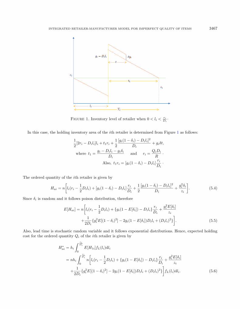
INTEGRATED RETAILER-MANUFACTURER MODEL FOR IMPERFECT QUALITY OF ITEMS 3467
Figure 1. Inventory level of retailer when 0 < 𝑙𝑖 < 𝑟𝑖
𝐷𝑖·
In this case, the holding inventory area of the 𝑖th retailer is determined from Figure 1 as follows:
12
[2𝑟𝑖 −𝐷𝑖𝑙𝑖]𝑙𝑖 + 𝑡1𝑟𝑖 +12
[𝑔𝑖(1− 𝛿𝑖)−𝐷𝑖𝑙𝑖]2
𝐷𝑖+ 𝑔𝑖𝛿𝑡,
where 𝑡1 =𝑔𝑖 −𝐷𝑖𝑙𝑖 − 𝑔𝑖𝛿𝑖
𝐷𝑖and 𝑟𝑖 =
𝑄𝑖𝐷𝑖
𝑅·
Also, 𝑡1𝑟𝑖 = [𝑔𝑖(1− 𝛿𝑖)−𝐷𝑖𝑙𝑖]𝑟𝑖
𝐷𝑖·
The ordered quantity of the 𝑖th retailer is given by
𝐻𝑎𝑖 = 𝑛
[𝑙𝑖(𝑟𝑖 −
12𝐷𝑖𝑙𝑖) + [𝑔𝑖(1− 𝛿𝑖)−𝐷𝑖𝑙𝑖]
𝑟𝑖
𝐷𝑖+
12
[𝑔𝑖(1− 𝛿𝑖)−𝐷𝑖𝑙𝑖]2
𝐷𝑖+
𝑔2𝑖 𝛿𝑖
𝑧𝑖
]. (5.4)
Since 𝛿𝑖 is random and it follows poison distribution, therefore
𝐸[𝐻𝑎𝑖] = 𝑛
[𝑙𝑖(𝑟𝑖 −
12𝐷𝑖𝑙𝑖) + {𝑔𝑖(1− 𝐸[𝛿𝑖])−𝐷𝑖𝑙𝑖}
𝑟𝑖
𝐷𝑖+
𝑔2𝑖 𝐸[𝛿𝑖]
𝑧𝑖
+1
2𝐷𝑖{𝑔2
𝑖 𝐸[(1− 𝛿𝑖)2]− 2𝑔𝑖(1− 𝐸[𝛿𝑖])𝐷𝑖𝑙𝑖 + (𝐷𝑖𝑙𝑖)2}]. (5.5)
Also, lead time is stochastic random variable and it follows exponential distributions. Hence, expected holdingcost for the ordered quantity 𝑄𝑖 of the 𝑖th retailer is given by
𝐻*𝑎𝑖 = ℎ𝑖
∫ 𝑟𝑖𝐷𝑖
0
𝐸[𝐻1𝑖]𝑓𝐿(𝑙𝑖)d𝑙𝑖
= 𝑛ℎ𝑖
∫ 𝑟𝑖𝐷𝑖
0
𝑛
[𝑙𝑖(𝑟𝑖 −
12𝐷𝑖𝑙𝑖) + {𝑔𝑖(1− 𝐸[𝛿𝑖])−𝐷𝑖𝑙𝑖}
𝑟𝑖
𝐷𝑖+
𝑔2𝑖 𝐸[𝛿𝑖]
𝑧𝑖
+1
2𝐷𝑖{𝑔2
𝑖 𝐸[(1− 𝛿𝑖)2]− 2𝑔𝑖(1− 𝐸[𝛿𝑖])𝐷𝑖𝑙𝑖 + (𝐷𝑖𝑙𝑖)2}]𝑓𝐿(𝑙𝑖)d𝑙𝑖. (5.6)

3468 D. BARMAN ET AL.
Figure 2. Inventory level of retailer when 𝑟𝑖
𝐷𝑖≤ 𝑙𝑖 ≤ (𝑟𝑖+𝑔𝑖)
𝐷𝑖·
5.1.2. When 𝑔𝑖 reaches late to the 𝑖th retailer and the lead time 𝑙𝑖 lies in the range 𝑟𝑖
𝐷𝑖≤ 𝑙𝑖 ≤ (𝑟𝑖+𝑔𝑖)
𝐷𝑖
Here order quantity reaches late to the 𝑖th retailer’s end. Shortages are occurred and they are used to satisfyback orders. Upon the arrival of order quantity, the retailer inspects all the items at a fixed screening rate 𝑧𝑖
and all defective items in each lot are discovered and returned to the manufacturer at the time of delivery ofthe next lot. Figure 2 illustrates the behavior of the inventory level over time for the retailer. Here batch 𝑔𝑖
is received at time 𝑙𝑖. Again, 𝑡, where 𝑡 = 𝑔𝑖
𝑧𝑖, is the completion time of the 100% screening process, 𝑡1 is the
period of time in which demand will be filled from inventory, and 𝑡2 is the period of time in which demand willbe back ordered. Among the 𝑔𝑖 units, 𝛿𝑔𝑖 units are defective and will be removed from inventory at time 𝑡.
In this case, the holding inventory area of the 𝑖th retailer is determined from Figure 2 and is described asfollows: As shortages occur, the amount of shortages will be (𝐷𝑖𝑙𝑖− 𝑟𝑖). Hence, (𝐷𝑖𝑙𝑖− 𝑟𝑖) units of items intendto satisfy the back orders in the cycle will be filled at rate of [𝑧𝑖(1− 𝛿𝑖)−𝐷𝑖]. We have
𝑡3 =𝐷𝑖𝑙𝑖 − 𝑟𝑖
𝑧𝑖(1− 𝛿𝑖)−𝐷𝑖,
and 𝑡2 =𝐷𝑖𝑙𝑖 − 𝑟𝑖
𝐷𝑖.
Hence back ordering area for 𝑖th cycle is given as follows:
12
(𝐷𝑖𝑙𝑖 − 𝑟𝑖)(𝑡2 + 𝑡3) =12
(𝐷𝑖𝑙𝑖 − 𝑟𝑖)𝐷𝑖𝑙𝑖 − 𝑟𝑖
𝐷𝑖+
12
(𝐷𝑖𝑙𝑖 − 𝑟𝑖)𝐷𝑖𝑙𝑖 − 𝑟𝑖
𝑧𝑖(1− 𝛿𝑖)−𝐷𝑖
=12
(𝐷𝑖𝑙𝑖 − 𝑟𝑖)2{
1𝐷𝑖
+1
𝑧𝑖(1− 𝛿𝑖 − 𝐷𝑖
𝑧𝑖)
}.
Thus, back ordered quantity of the 𝑖th retailer is given by
𝐵 = 𝑛
[12
(𝐷𝑖𝑙𝑖 − 𝑟𝑖)2{
1𝐷𝑖
+1
𝑧𝑖(1− 𝛿𝑖 − 𝐷𝑖
𝑧𝑖)
}]. (5.7)

INTEGRATED RETAILER-MANUFACTURER MODEL FOR IMPERFECT QUALITY OF ITEMS 3469
Now, 𝛿𝑖 is a random variable. Hence,
𝐸[𝐵] = 𝑛
[12
(𝐷𝑖𝑙𝑖 − 𝑟𝑖)2{
1𝐷𝑖
+1𝑧𝑖
𝐸
[1
(1− 𝛿𝑖 − 𝐷𝑖
𝑧𝑖)
]}].
Also, lead time is a stochastic random variable and it follows exponential distribution. Hence, expected backordering cost for the ordered quantity 𝑄𝑖 of the 𝑖th retailer is
𝐵*𝑖 = 𝑏𝑖
∫ (𝑟𝑖+𝑔𝑖)𝐷𝑖
𝑟𝑖𝐷𝑖
𝐸[𝐵]𝑓𝐿(𝑙𝑖)d𝑙𝑖
=𝑛𝑏𝑖
2
∫ (𝑟𝑖+𝑔𝑖)𝐷𝑖
𝑟𝑖𝐷𝑖
{1𝐷𝑖
+1𝑧𝑖
𝐸
[1
(1− 𝛿𝑖 − 𝐷𝑖
𝑧𝑖)
]}(𝐷𝑖𝑙𝑖 − 𝑟𝑖)2𝑓𝐿(𝑙𝑖)d𝑙𝑖.
After time 𝑡3, the time to fill (𝐷𝑖𝑙𝑖 − 𝑟𝑖), the maximum shortage level for 𝑖th cycle, the inventory level willbe reduced by (𝐷𝑖𝑙𝑖 − 𝑟𝑖) + 𝑡3𝐷𝑖 = 𝑧𝑖(1−𝛿𝑖)(𝐷𝑖𝑙𝑖−𝑟𝑖)
𝑧𝑖(1−𝛿𝑖)−𝐷𝑖· At time 𝑡 (which is 𝑔𝑖
𝑧𝑖), 𝛿𝑔𝑖 defective units will be removed
from the inventory. Thus, the holding area for 𝑖th cycle is as follows
𝑡1 =𝑔𝑖(1− 𝛿𝑖)− (𝐷𝑖𝑙𝑖 − 𝑟𝑖)
𝐷𝑖·
Total holding inventory area is determined from Figure 2, which is
𝑟2𝑖
2𝐷𝑖+ 𝑡1𝑟𝑖 +
{𝑔𝑖(1− 𝛿𝑖)−
12
𝑧𝑖(1− 𝛿𝑖)(𝐷𝑖𝑙𝑖 − 𝑟𝑖)𝑧𝑖(1− 𝛿𝑖)−𝐷𝑖
}𝐷𝑖𝑙𝑖 − 𝑟𝑖
𝑧𝑖(1− 𝛿𝑖)−𝐷𝑖+
𝑔2𝑖 𝛿𝑖
𝑧𝑖
+12
{𝑔𝑖(1− 𝛿𝑖)−
𝑧𝑖(1− 𝛿𝑖)(𝐷𝑖𝑙𝑖 − 𝑟𝑖)𝑧𝑖(1− 𝛿𝑖)−𝐷𝑖
}{𝑔𝑖(1− 𝛿𝑖)− (𝐷𝑖𝑙𝑖 − 𝑟𝑖)
𝐷𝑖− 𝐷𝑖𝑙𝑖 − 𝑟𝑖
𝑧𝑖(1− 𝛿𝑖)−𝐷𝑖
}.
The ordered quantity of the 𝑖th retailer 𝑄𝑖 is given by
𝐻𝑏𝑖 = 𝑛
[𝑟2𝑖
2𝐷𝑖+
𝑔2𝑖 𝛿𝑖
𝑧𝑖+
𝑟𝑖
𝐷𝑖{𝑔𝑖(1− 𝛿𝑖)− (𝐷𝑖𝑙𝑖 − 𝑟𝑖)}+
12
𝑔𝑖(𝐷𝑖𝑙𝑖 − 𝑟𝑖)(1− 𝛿𝑖)𝑧𝑖(1− 𝛿𝑖 − 𝐷𝑖
𝑧𝑖)
+12
{𝑔2
𝑖 (1− 𝛿𝑖)2
𝐷𝑖− 𝑔𝑖(1− 𝛿𝑖)2(𝐷𝑖𝑙𝑖 − 𝑟𝑖)
𝐷𝑖(1− 𝛿𝑖 − 𝐷𝑖
𝑧𝑖)
− 𝑔𝑖(1− 𝛿𝑖)(𝐷𝑖𝑙𝑖 − 𝑟𝑖)𝐷𝑖
+(𝐷𝑖𝑙𝑖 − 𝑟𝑖)2(1− 𝛿𝑖)
𝐷𝑖(1− 𝛿𝑖 − 𝐷𝑖
𝑧𝑖)
}].
(5.8)
Now, 𝛿𝑖 is random and it follows poison distribution. Hence
𝐸[𝐻𝑏𝑖] = 𝑛
[𝑟2𝑖
2𝐷𝑖+
𝑔2𝑖 𝐸[𝛿𝑖]
𝑧𝑖+
𝑟𝑖
𝐷𝑖{𝑔𝑖(1− 𝐸[𝛿𝑖])− (𝐷𝑖𝑙𝑖 − 𝑟𝑖)}+
𝑔𝑖(𝐷𝑖𝑙𝑖 − 𝑟𝑖)2𝑧𝑖
𝐸
[(1− 𝛿𝑖)
(1− 𝛿𝑖 − 𝐷𝑖
𝑧𝑖)
]+
12
{𝑔2
𝑖 𝐸[(1− 𝛿𝑖)2]𝐷𝑖
− 𝑔𝑖(𝐷𝑖𝑙𝑖 − 𝑟𝑖)𝐷𝑖
𝐸
[(1− 𝛿𝑖)2
(1− 𝛿𝑖 − 𝐷𝑖
𝑧𝑖)
]− 𝑔𝑖𝐸[(1− 𝛿𝑖)](𝐷𝑖𝑙𝑖 − 𝑟𝑖)
𝐷𝑖
+(𝐷𝑖𝑙𝑖 − 𝑟𝑖)2
𝐷𝑖𝐸
[(1− 𝛿𝑖)
(1− 𝛿𝑖 − 𝐷𝑖
𝑧𝑖)
]}]. (5.9)

3470 D. BARMAN ET AL.
Figure 3. Inventory level of retailer when (𝑟𝑖+𝑔𝑖)𝐷𝑖
≤ 𝑙𝑖 ≤ ∞·
Also, lead time is stochastic random variable and it follows exponential distributions. Hence, expected holdingcost for the ordered quantity 𝑄𝑖 of the 𝑖th retailer is as follows:
𝐻*𝑏𝑖 = ℎ𝑖
∫ (𝑟𝑖+𝑔𝑖)𝐷𝑖
𝑟𝑖𝐷𝑖
𝐸[𝐻2𝑖]𝑓𝐿(𝑙𝑖)d𝑙𝑖
= 𝑛ℎ𝑖
∫ (𝑟𝑖+𝑔𝑖)𝐷𝑖
𝑟𝑖𝐷𝑖
[𝑟2𝑖
2𝐷𝑖+
𝑔2𝑖 𝐸[𝛿𝑖]
𝑧𝑖+
𝑟𝑖
𝐷𝑖{𝑔𝑖(1− 𝐸[𝛿𝑖])− (𝐷𝑖𝑙𝑖 − 𝑟𝑖)}+
𝑔𝑖(𝐷𝑖𝑙𝑖 − 𝑟𝑖)2𝑧𝑖
𝐸
[(1− 𝛿𝑖)
(1− 𝛿𝑖 − 𝐷𝑖
𝑧𝑖)
]+
12
{𝑔2
𝑖 𝐸[(1− 𝛿𝑖)2]𝐷𝑖
− 𝑔𝑖(𝐷𝑖𝑙𝑖 − 𝑟𝑖)𝐷𝑖
𝐸
[(1− 𝛿𝑖)2
(1− 𝛿𝑖 − 𝐷𝑖
𝑧𝑖)
]− 𝑔𝑖𝐸[(1− 𝛿𝑖)](𝐷𝑖𝑙𝑖 − 𝑟𝑖)
𝐷𝑖
+(𝐷𝑖𝑙𝑖 − 𝑟𝑖)2
𝐷𝑖𝐸
[(1− 𝛿𝑖)
(1− 𝛿𝑖 − 𝐷𝑖
𝑧𝑖)
]}]𝑓𝐿(𝑙𝑖)d𝑙𝑖. (5.10)
It is assumed that during this delay period, the batches remain in the manufacturer’s stock house. So it causesan extra holding cost to the manufacturer. The extra inventory for this delayed delivery is
∑𝑁𝑖=1
𝑔𝑖(1−𝛿𝑖)(𝐷𝑖𝑙𝑖−𝑟𝑖)𝐷𝑖
:
𝑀𝑐 =𝑁∑
𝑖=1
𝑔𝑖(1− 𝛿𝑖)(𝐷𝑖𝑙𝑖 − 𝑟𝑖)𝐷𝑖
,
𝐸[𝑀𝑐] =𝑁∑
𝑖=1
𝑔𝑖𝐸[(1− 𝛿𝑖)](𝐷𝑖𝑙𝑖 − 𝑟𝑖)𝐷𝑖
·
Therefore, in this scenario, the extra holding cost paid by manufacturer is given by
ℎ𝑣
𝑁∑𝑖=1
∫ (𝑟𝑖+𝑔𝑖)𝐷𝑖
𝑟𝑖𝐷𝑖
𝑛𝑔𝑖𝐸[(1− 𝛿𝑖)](𝐷𝑖𝑙𝑖 − 𝑟𝑖)𝐷𝑖
𝑓𝐿(𝑙𝑖)d𝑙𝑖. (5.11)
INTEGRATED RETAILER-MANUFACTURER MODEL FOR IMPERFECT QUALITY OF ITEMS 3471
5.1.3. When 𝑔𝑖 reaches late to the 𝑖th retailer and the lead time 𝑙𝑖 lies in the range (𝑟𝑖+𝑔𝑖)𝐷𝑖
≤ 𝑙𝑖 ≤ ∞In this case, only shortages occur at the retailer’s end. From Figure 3, shortage area of the 𝑖th retailer is
obtained as follows:
𝐻𝑐𝑖 = 𝑛
[𝑔2
𝑖
2𝐷𝑖+ 𝑔𝑖
{(𝐷𝑖𝑙𝑖 − 𝑔𝑖 − 𝑟𝑖)
𝐷𝑖
}]= 𝑛
{𝑔𝑖
𝐷𝑖(𝐷𝑖𝑙𝑖 − 𝑟𝑖)−
𝑔2𝑖
2𝐷𝑖
}. (5.12)
Also, lead time is stochastic random variable and it follows exponential distributions. Hence, expected shortagecost for the ordered quantity 𝑄𝑖 of the 𝑖th retailer is given by
𝐻*𝑐𝑖 = ℎ𝑖
∫ ∞
(𝑟𝑖+𝑔𝑖)𝐷𝑖
𝐸[𝐻3𝑖]𝑓𝐿(𝑙𝑖)d𝑙𝑖 = 𝑛𝑐𝑖
∫ ∞
(𝑟𝑖+𝑔𝑖)𝐷𝑖
{𝑔𝑖
𝐷𝑖(𝐷𝑖𝑙𝑖 − 𝑟𝑖)−
𝑔2𝑖
2𝐷𝑖
}𝑓𝐿(𝑙𝑖)d𝑙𝑖. (5.13)
It is assumed that during this delay period, the batches remain in the manufacturer’s stock house. So it causesan extra holding cost to the manufacturer. The extra inventory for this delayed delivery is
∑𝑁𝑖=1
𝑔𝑖(1−𝛿𝑖)(𝐷𝑖𝑙𝑖−𝑟𝑖)𝐷𝑖
:
𝑀𝑐 =𝑁∑
𝑖=1
𝑔𝑖(1− 𝛿𝑖)(𝐷𝑖𝑙𝑖 − 𝑟𝑖)𝐷𝑖
,
𝐸[𝑀𝑐] =𝑁∑
𝑖=1
𝑔𝑖𝐸[(1− 𝛿𝑖)](𝐷𝑖𝑙𝑖 − 𝑟𝑖)𝐷𝑖
.
Therefore, in this scenario, the extra holding cost paid by manufacturer is
ℎ𝑣
𝑁∑𝑖=1
∫ ∞
(𝑟𝑖+𝑔𝑖)𝐷𝑖
𝑛𝑔𝑖𝐸[(1− 𝛿𝑖)](𝐷𝑖𝑙𝑖 − 𝑟𝑖)𝐷𝑖
𝑓𝐿(𝑙𝑖)d𝑙𝑖. (5.14)
5.2. Mathematical model formulation for manufacturer
Once retailers order is placed, the manufacturer start to begin production and produces the total orderquantity
∑𝑁𝑖=1 𝑄𝑖 of all retailers in 𝑛 lots at one set up at a production rate 𝑅, and a finite number of units
are added to the inventory until the production run has been completed. The manufacturer produces the itemsin a lot size of 𝑄, where 𝑄 =
∑𝑁𝑖=1 𝑄𝑖 and 𝑄𝑖 = 𝑛𝑔𝑖 in each production of cycle length 𝑄
𝑅 and the retailerswill receive the supply in each of size 𝑔𝑖 for 𝑖th retailer. The first lot of size
∑𝑁𝑖=1 𝑔𝑖 is ready for shipment after
time∑𝑁
𝑖=1 𝑔𝑖
𝑅 just after starting of the production run, and the manufacturer continues making the delivery onaverage every 𝐸[𝑇 ] = 𝐸[(𝑄 − 𝛿)/𝐷], where 𝐸[(𝑄 − 𝛿)/𝐷] =
∑𝑁𝑖=1 𝐸[(𝑄𝑖 − 𝑛𝛿𝑖)/𝐷𝑖], units of time until the
inventory level falls to zero.Here, the production rate of manufacturer’s non-defective items is greater than the retailer’s demand rate,
so manufacturer’s inventory level will increase gradually. When the total required amount 𝑄 is fulfilled, themanufacturer stops producing items immediately.
Therefore, the manufacturer’s inventory per production cycle can be obtained by subtracting the accumulatedretailer inventory level from the accumulated manufacturer inventory level as follows.Therefore, the total extra holding cost for the manufacturer, from both case (ii) and case (iii), is as follows:
ℎ𝑣
𝑁∑𝑖=1
∫ ∞
𝑟𝑖𝐷𝑖
𝑛𝑔𝑖𝐸[(1− 𝛿𝑖)](𝐷𝑖𝑙𝑖 − 𝑟𝑖)𝐷𝑖
𝑓𝐿(𝑙𝑖)d𝑙𝑖. (5.15)
In Figure 4, trapezium ABCD represents the joint inventory of the manufacturer-retailer system. The averageinventory of the system is obtained as follows:
12
[∑𝑁𝑖=1 𝑔𝑖
𝑅+
{𝑄− 𝛿
𝐷+
∑𝑁𝑖=1 𝑔𝑖
𝑅− 𝑄
𝑅
}]𝑄
𝐷
𝑄− 𝛿=
𝐷𝑄
(𝑄− 𝛿)
∑𝑁𝑖=1 𝑔𝑖
𝑅+
𝑄
2
(1− 𝐷
𝑅
𝑄
(𝑄− 𝛿)
).
(5.16)

3472 D. BARMAN ET AL.
Figure 4. Inventory level of retailer when 𝑟𝑖
𝐷𝑖≤ 𝑙𝑖 ≤ (𝑟𝑖+𝑄𝑖)
𝐷𝑖·
Average holding area of 𝑁 retailers is
𝑁∑𝑖=1
𝑔2𝑖
2𝐷𝑖
𝐷𝑖
𝑛(𝑔𝑖 − 𝛿𝑖)=
𝑁∑𝑖=1
𝑔2𝑖
2𝑛(𝑔𝑖 − 𝛿𝑖)· (5.17)
So, average holding area of manufacturer is
𝐻𝑣 =𝐷𝑄
(𝑄− 𝛿)
∑𝑁𝑖=1 𝑔𝑖
𝑅+
𝑄
2
(1− 𝐷
𝑅
𝑄
(𝑄− 𝛿)
)−
𝑁∑𝑖=1
𝑔2𝑖
2𝑛(𝑔𝑖 − 𝛿𝑖)· (5.18)
Hence,
𝐸[𝐻𝑣] = 𝐸
[𝐷𝑄
(𝑄− 𝛿)
]∑𝑁𝑖=1 𝑔𝑖
𝑅+
𝑄
2
{1− 𝐷
𝑅𝐸
[𝑄
(𝑄− 𝛿)
]}− 𝐸
[ 𝑁∑𝑖=1
𝑔2𝑖
2𝑛(𝑔𝑖 − 𝛿𝑖)
]
= 𝐸
[ 𝑁∑𝑖=1
𝑄𝑖𝐷𝑖
𝑄𝑖 − 𝑛𝛿𝑖
] 𝑁∑𝑖=1
𝑔𝑖
𝑅+
𝑄
2
{1− 𝐷
𝑅𝐸
[ 𝑁∑𝑖=1
𝑄𝑖
𝑄𝑖 − 𝑛𝛿𝑖
]}− 𝐸
[ 𝑁∑𝑖=1
𝑔2𝑖
2𝑛(𝑔𝑖 − 𝛿𝑖)
]
=𝑁∑
𝑖=1
𝑄𝑖𝐷𝑖
𝑛𝑔𝑖(1− 𝛾𝑖)
𝑁∑𝑖=1
𝑔𝑖
𝑅+
𝑄
2
{1− 𝐷
𝑅
𝑁∑𝑖=1
𝑄𝑖
𝑛𝑔𝑖(1− 𝛾𝑖)
}−
𝑁∑𝑖=1
𝑔2𝑖
2𝑛𝑔𝑖(1− 𝛾𝑖)
=𝑁∑
𝑖=1
𝑔𝑖
𝑅
𝑁∑𝑖=1
𝐷𝑖
(1− 𝛾𝑖)+
𝑄
2
{1− 𝐷
𝑅
𝑁∑𝑖=1
1(1− 𝛾𝑖)
}−
𝑁∑𝑖=1
𝑔𝑖
2𝑛(1− 𝛾𝑖)· (5.19)
5.3. Decentralized model
Within the decentralized version situation, the manufacturer and the retailers make their decisions indepen-dently with the intention to enhance their own profits. Here we incorporate a Stackelberg gaming structurewherein the retailers act as the leader and the manufacturer as the follower. The manufacturer sets the wide
INTEGRATED RETAILER-MANUFACTURER MODEL FOR IMPERFECT QUALITY OF ITEMS 3473
variety of shipments and greening development stage of the product. Then, taking those reaction functions intoconsideration, the retailers determine optimal retail expenses of the product and batch sizes.
5.3.1. Retailer’s profit function
The expected total cost of 𝑖th retailer includes ordering cost, screening cost, transportation cost, holdingcost, back order cost, shortage cost. Thus Expected total profit for the 𝑖th retailer is
EAC𝑇𝑖 (𝑔𝑖, 𝑝𝑖) = 𝑝𝑖𝑄𝑖 − 𝑤ℎ𝑄𝑖 −𝐴𝑖 − 𝑑𝑖𝑄𝑖 − 𝑛𝑇𝑝 −𝐻*
𝑎𝑖 −𝐻*𝑏𝑖 −𝐵*𝑖 −𝐻*
𝑐𝑖
= 𝑝𝑖𝑄𝑖 − 𝑤ℎ𝑄𝑖 −𝐴𝑖 − 𝑑𝑄𝑖 − 𝑛𝑇𝑝 − 𝑛ℎ𝑖
∫ 𝑟𝑖𝐷𝑖
0
[𝑙𝑖
(𝑟𝑖 −
12𝐷𝑖𝑙𝑖
)+ {𝑔𝑖(1− 𝐸[𝛿𝑖])−𝐷𝑖𝑙𝑖}
𝑟𝑖
𝐷𝑖
+𝑔2
𝑖 𝐸[𝛿𝑖]𝑧𝑖
+1
2𝐷𝑖{𝑔2
𝑖 𝐸[(1− 𝛿𝑖)2]− 2𝑔𝑖(1− 𝐸[𝛿𝑖])𝐷𝑖𝑙𝑖 + (𝐷𝑖𝑙𝑖)2}]𝑓𝐿(𝑙𝑖)d𝑙𝑖
−𝑛ℎ𝑖
∫ (𝑟𝑖+𝑔𝑖)𝐷𝑖
𝑟𝑖𝐷𝑖
[𝑟2𝑖
2𝐷𝑖+
𝑔2𝑖 𝐸[𝛿𝑖]
𝑧𝑖+
𝑟𝑖
𝐷𝑖{𝑔𝑖(1− 𝐸[𝛿𝑖])− (𝐷𝑖𝑙𝑖 − 𝑟𝑖)}+
𝑔𝑖(𝐷𝑖𝑙𝑖 − 𝑟𝑖)2𝑧𝑖
𝐸
[(1− 𝛿𝑖)
(1− 𝛿𝑖 − 𝐷𝑖
𝑧𝑖)
]+
12
{𝑔2
𝑖 𝐸[(1− 𝛿𝑖)2]𝐷𝑖
− 𝑔𝑖(𝐷𝑖𝑙𝑖 − 𝑟𝑖)𝐷𝑖
𝐸
[(1− 𝛿𝑖)2
(1− 𝛿𝑖 − 𝐷𝑖
𝑧𝑖)
]−𝑔𝑖𝐸[(1− 𝛿𝑖)](𝐷𝑖𝑙𝑖 − 𝑟𝑖)
𝐷𝑖+
(𝐷𝑖𝑙𝑖 − 𝑟𝑖)2
𝐷𝑖𝐸
[(1− 𝛿𝑖)
(1− 𝛿𝑖 − 𝐷𝑖
𝑧𝑖)
]}]𝑓𝐿(𝑙𝑖)d𝑙𝑖
−𝑛𝑏𝑖
2
∫ (𝑟𝑖+𝑔𝑖)𝐷𝑖
𝑟𝑖𝐷𝑖
{1𝐷𝑖
+1𝑧𝑖
𝐸
[1
(1− 𝛿𝑖 − 𝐷𝑖
𝑧𝑖)
]}(𝐷𝑖𝑙𝑖 − 𝑟𝑖)2𝑓𝐿(𝑙𝑖)d𝑙𝑖
−𝑛𝑐𝑖
∫ ∞
(𝑟𝑖+𝑔𝑖)𝐷𝑖
{𝑔𝑖
𝐷𝑖(𝐷𝑖𝑙𝑖 − 𝑟𝑖)−
𝑔2𝑖
2𝐷𝑖
}𝑓𝐿(𝑙𝑖)d𝑙𝑖.
Thus average expected profit of the 𝑖th retailer is
EAC𝑖(𝑔𝑖, 𝑝𝑖) =𝐷𝑖
(1− 𝛾𝑖)(𝑝𝑖 − 𝑤ℎ − 𝑑𝑖)−
𝐷𝑖
𝑛𝑔𝑖(1− 𝛾𝑖)(𝐴𝑖 + 𝑛𝑇𝑝)
− ℎ𝑖
1− 𝛾𝑖
∫ 𝑟𝑖𝐷𝑖
0
[𝑟𝑖(1− 𝐸[𝛿𝑖])−
𝐷𝑖𝑙𝑖2𝑔𝑖
+𝐷𝑖𝑔𝑖𝐸[𝛿𝑖]
𝑧𝑖+
12{𝑔𝑖𝐸[(1− 𝛿𝑖)2]− 2(1− 𝐸[𝛿𝑖])𝐷𝑖𝑙𝑖
+(𝐷𝑖𝑙𝑖)2
𝑔𝑖}]𝑓𝐿(𝑙𝑖)d𝑙𝑖 −
ℎ𝑖
1− 𝛾𝑖
∫ (𝑟𝑖+𝑔𝑖)𝐷𝑖
𝑟𝑖𝐷𝑖
[𝑟2𝑖
2𝑔𝑖+
𝐷𝑖𝑔𝑖𝐸[𝛿𝑖]𝑧𝑖
+ 𝑟𝑖{(1− 𝐸[𝛿𝑖])−(𝐷𝑖𝑙𝑖 − 𝑟𝑖)
𝑔𝑖}
+𝐷𝑖(𝐷𝑖𝑙𝑖 − 𝑟𝑖)
2𝑧𝑖𝐸
[(1− 𝛿𝑖)
(1− 𝛿𝑖 − 𝐷𝑖
𝑧𝑖)
]+
12
{𝑔𝑖𝐸[(1− 𝛿𝑖)2]− (𝐷𝑖𝑙𝑖 − 𝑟𝑖)𝐸
[(1− 𝛿𝑖)2
(1− 𝛿𝑖 − 𝐷𝑖
𝑧𝑖)
]−𝐸[(1− 𝛿𝑖)](𝐷𝑖𝑙𝑖 − 𝑟𝑖) +
(𝐷𝑖𝑙𝑖 − 𝑟𝑖)2
𝑔𝑖𝐸
[(1− 𝛿𝑖)
(1− 𝛿𝑖 − 𝐷𝑖
𝑧𝑖)
]}]𝑓𝐿(𝑙𝑖)d𝑙𝑖
− 𝑏𝑖
2𝑔𝑖(1− 𝛾𝑖)
∫ (𝑟𝑖+𝑔𝑖)𝐷𝑖
𝑟𝑖𝐷𝑖
{1 +
𝐷𝑖
𝑧𝑖𝐸
[1
(1− 𝛿𝑖 − 𝐷𝑖
𝑧𝑖)
]}(𝐷𝑖𝑙𝑖 − 𝑟𝑖)2𝑓𝐿(𝑙𝑖)d𝑙𝑖
− 𝑐𝑖
1− 𝛾𝑖
∫ ∞
(𝑟𝑖+𝑔𝑖)𝐷𝑖
{(𝐷𝑖𝑙𝑖 − 𝑟𝑖)−
𝑔2𝑖
2
}𝑓𝐿(𝑙𝑖)d𝑙𝑖
=𝐷𝑖
(1− 𝛾𝑖)(𝑝𝑖 − 𝑤ℎ − 𝑑𝑖)−
𝐷𝑖
𝑛𝑔𝑖(1− 𝛾𝑖)(𝐴𝑖 + 𝑛𝑇𝑝)

3474 D. BARMAN ET AL.
− ℎ𝑖
1− 𝛾𝑖
∫ 𝑟𝑖𝐷𝑖
0
[𝑟𝑖(1− 𝐸[𝛿𝑖])−
𝐷𝑖𝑙𝑖2𝑔𝑖
+𝐷𝑖𝑔𝑖𝐸[𝛿𝑖]
𝑧𝑖+
12
{𝑔𝑖𝐸[(1− 𝛿𝑖)2]− 2(1− 𝐸[𝛿𝑖])𝐷𝑖𝑙𝑖
+(𝐷𝑖𝑙𝑖)2
𝑔𝑖
}]𝑓𝐿(𝑙𝑖)d𝑙𝑖 −
ℎ𝑖
1− 𝛾𝑖
∫ (𝑟𝑖+𝑔𝑖)𝐷𝑖
𝑟𝑖𝐷𝑖
[𝑟2𝑖
2𝑔𝑖+
𝐷𝑖𝑔𝑖𝐸[𝛿𝑖]𝑧𝑖
+ 𝑟𝑖{(1− 𝐸[𝛿𝑖])−(𝐷𝑖𝑙𝑖 − 𝑟𝑖)
𝑔𝑖}
+𝐷𝑖(𝐷𝑖𝑙𝑖 − 𝑟𝑖)
2𝑧𝑖𝐴1𝑖 +
12
{𝑔𝑖𝐸[(1− 𝛿𝑖)2]− (𝐷𝑖𝑙𝑖 − 𝑟𝑖)𝐴2𝑖 − 𝐸[(1− 𝛿𝑖)](𝐷𝑖𝑙𝑖 − 𝑟𝑖)
+(𝐷𝑖𝑙𝑖 − 𝑟𝑖)2
𝑔𝑖𝐴1𝑖
}]𝑓𝐿(𝑙𝑖)d𝑙𝑖 −
𝑏𝑖
2𝑔𝑖(1− 𝛾𝑖)
∫ (𝑟𝑖+𝑔𝑖)𝐷𝑖
𝑟𝑖𝐷𝑖
{1 +
𝐷𝑖
𝑧𝑖𝐴3𝑖
}(𝐷𝑖𝑙𝑖 − 𝑟𝑖)2𝑓𝐿(𝑙𝑖)d𝑙𝑖
− 𝑐𝑖
1− 𝛾𝑖
∫ ∞
(𝑟𝑖+𝑔𝑖)𝐷𝑖
{(𝐷𝑖𝑙𝑖 − 𝑟𝑖)−
𝑔2𝑖
2
}𝑓𝐿(𝑙𝑖)d𝑙𝑖, (5.20)
where
𝐴1𝑖 = 𝐸
[(1− 𝛿𝑖)
(1− 𝛿𝑖 − 𝐷𝑖
𝑧𝑖)
], 𝐴2𝑖 = 𝐸
[(1− 𝛿𝑖)2
(1− 𝛿𝑖 − 𝐷𝑖
𝑧𝑖)
], and 𝐴3𝑖 = 𝐸
[1
(1− 𝛿𝑖 − 𝐷𝑖
𝑧𝑖)
].
Proposition 5.1. If 𝐸[𝛿𝑖] < 1− 𝐷𝑖
𝑧𝑖, then the average expected profit of the 𝑖th retailer will be concave in 𝑔𝑖 for
given 𝑝𝑖, if2𝐷𝑖(𝐴𝑖+𝑛𝑇𝑝)
𝑛(1−𝛾𝑖)+ ℎ𝑖
1−𝛾𝑖
∫ 𝑟𝑖𝐷𝑖
0
[(𝐷𝑖𝑙𝑖)2−𝐷𝑖𝑙𝑖
]𝑓𝐿(𝑙𝑖)d𝑙𝑖 + ℎ𝑖
1−𝛾𝑖
∫ (𝑟𝑖+𝑔𝑖)𝐷𝑖
𝑟𝑖𝐷𝑖
[2(𝑑𝑖𝑙𝑖−𝑟𝑖)2𝐴1𝑖−2𝑟𝑖(𝑑𝑖𝑙𝑖−𝑟𝑖)2 +𝑟2
𝑖
]𝑓𝐿(𝑙𝑖)d𝑙𝑖 +
𝑏𝑖
1−𝛾𝑖
∫ (𝑟𝑖+𝑔𝑖)𝐷𝑖
𝑟𝑖𝐷𝑖
𝐴3𝑖
(1 + 𝐷𝑖
𝑧𝑖
)(𝐷𝑖𝑙𝑖 − 𝑟𝑖)2𝑓𝐿(𝑙𝑖)d𝑙𝑖 > 0.
Proof. Differentiating profit function with respect to 𝑔𝑖, we obtain
𝜕EAC𝑖(𝑔𝑖, 𝑝𝑖)𝜕𝑔𝑖
=𝐷𝑖(𝐴𝑖 + 𝑛𝑇𝑝)𝑛𝑔2
𝑖 (1− 𝛾𝑖)− ℎ𝑖
1− 𝛾𝑖
∫ 𝑟𝑖𝐷𝑖
0
[𝐷𝑖𝑙𝑖2𝑔2
𝑖
+𝐷𝑖𝐸[𝛿𝑖]
𝑧𝑖+
12𝐸[(1− 𝛿𝑖)2]− (𝐷𝑖𝑙𝑖)2
2𝑔2𝑖
]𝑓𝐿(𝑙𝑖)d𝑙𝑖
− ℎ𝑖
1− 𝛾𝑖
∫ 𝑟𝑖+𝑔𝑖𝐷𝑖
𝑟𝑖𝐷𝑖
[− 𝑟𝑖
2𝑔2𝑖
+𝐷𝑖𝐸[𝛿𝑖]
𝑧𝑖+
𝑟𝑖(𝐷𝑖𝑙𝑖 − 𝑟𝑖)𝑔2
𝑖
+12
(1− 𝐸[𝛿𝑖])2
− (𝐷𝑖𝑙𝑖 − 𝑟𝑖)2
2𝑔2𝑖
𝐴1𝑖
]𝑓𝐿(𝑙𝑖)d𝑙𝑖 +
𝑏𝑖
2𝑔2𝑖 (1− 𝛾𝑖)
∫ 𝑟𝑖+𝑔𝑖𝐷𝑖
𝑟𝑖𝐷𝑖
(1 +
𝐷𝑖
𝑧𝑖𝐴3𝑖
)(𝐷𝑖𝑙𝑖 − 𝑟𝑖)2𝑓𝐿(𝑙𝑖)d𝑙𝑖,
𝜕2EAC𝑖(𝑔𝑖, 𝑝𝑖)𝜕𝑔2
𝑖
= − 2𝐷𝑖
𝑛𝑔3𝑖 (1− 𝛾𝑖)
(𝐴𝑖 + 𝑛𝑇𝑝)− ℎ𝑖
𝑔3𝑖 (1− 𝛾𝑖
∫ 𝑟𝑖𝐷𝑖
0
[(𝐷𝑖𝑙𝑖)2 −𝐷𝑖𝑙𝑖
]𝑓𝐿(𝑙𝑖)d𝑙𝑖
− ℎ𝑖
𝑔3𝑖 (1− 𝛾𝑖
∫ (𝑟𝑖+𝑔𝑖𝐷𝑖
𝑟𝑖𝐷𝑖
[2(𝑑𝑖𝑙𝑖 − 𝑟𝑖)2𝐴1𝑖 − 2𝑟𝑖(𝑑𝑖𝑙𝑖 − 𝑟𝑖)2 + 𝑟2
𝑖
]𝑓𝐿(𝑙𝑖)d𝑙𝑖
− 𝑏𝑖
𝑔3𝑖 (1− 𝛾𝑖)
∫ (𝑟𝑖+𝑔𝑖𝐷𝑖
𝑟𝑖𝐷𝑖
𝐴3𝑖
(1 +
𝐷𝑖
𝑧𝑖
)(𝐷𝑖𝑙𝑖 − 𝑟𝑖)2𝑓𝐿(𝑙𝑖)d𝑙𝑖.
Thus, if 𝐸[𝛿𝑖] < 1− 𝐷𝑖
𝑧𝑖, then the average expected profit function of the 𝑖th retailer is concave in 𝑔𝑖 for given 𝑝𝑖,
if 𝜕2EAC𝑖(𝑔𝑖,𝑝𝑖)𝜕𝑔2
𝑖is negative. This implies 2𝐷𝑖(𝐴𝑖+𝑛𝑇𝑝)
𝑛(1−𝛾𝑖)+ ℎ𝑖
1−𝛾𝑖
∫ 𝑟𝑖𝐷𝑖
0
[(𝐷𝑖𝑙𝑖)2−𝐷𝑖𝑙𝑖
]𝑓𝐿(𝑙𝑖)d𝑙𝑖 + ℎ𝑖
1−𝛾𝑖
∫ (𝑟𝑖+𝑔𝑖)𝐷𝑖
𝑟𝑖𝐷𝑖
[2(𝑑𝑖𝑙𝑖−
𝑟𝑖)2𝐴1𝑖 − 2𝑟𝑖(𝑑𝑖𝑙𝑖 − 𝑟𝑖)2 + 𝑟2𝑖
]𝑓𝐿(𝑙𝑖)d𝑙𝑖 + 𝑏𝑖
1−𝛾𝑖
∫ (𝑟𝑖+𝑔𝑖)𝐷𝑖
𝑟𝑖𝐷𝑖
𝐴3𝑖
(1 + 𝐷𝑖
𝑧𝑖
)(𝐷𝑖𝑙𝑖 − 𝑟𝑖)
2𝑓𝐿(𝑙𝑖)d𝑙𝑖 > 0. ⊓⊔
INTEGRATED RETAILER-MANUFACTURER MODEL FOR IMPERFECT QUALITY OF ITEMS 3475
Proposition 5.2. If 𝐸[𝛿𝑖] < 1 − 𝐷𝑖
𝑧𝑖and 𝐷𝑖𝑙𝑖 > 𝑟𝑖, then the average expected profit of the 𝑖th retailer will
be concave in 𝑝𝑖 for given 𝑔𝑖 if 𝛽𝑖
1−𝛾𝑖+ 𝛽2
𝑖 ℎ𝑖
1−𝛾𝑖
[ ∫ 𝑟𝑖𝐷𝑖
0𝑙2𝑖𝑔𝑖
𝑓𝐿(𝑙𝑖)d𝑙𝑖 +∫ (𝑟𝑖+𝑔𝑖)
𝐷𝑖𝑟𝑖𝐷𝑖
𝐴1𝑖𝑙𝑖( 𝑖2𝑧𝑖
+ 1𝑔𝑖
)𝑓𝐿(𝑙𝑖)d𝑙𝑖
]+ 𝑏𝑖𝛽𝑖
2𝑔𝑖(1−𝛾𝑖)𝐽11 > 0.
Proof. Differentiating profit function with respect to 𝑔𝑖, we obtain
𝜕EAC𝑖(𝑔𝑖, 𝑝𝑖)𝜕𝑝𝑖
= − 𝛽𝑖
1− 𝛾𝑖(𝑝𝑖 − 𝑤ℎ − 𝑑𝑖) +
𝛽𝑖(𝐴𝑖 + 𝑛𝑇𝑝)𝑛𝑔𝑖(1− 𝛾𝑖)
− ℎ𝑖
1− 𝛾𝑖
∫ 𝑟𝑖𝐷𝑖
0
[𝛽𝑖
𝑙𝑖2𝑔𝑖 −
𝛽𝑖𝑔𝑖𝐸[𝛿𝑖]𝑧𝑖
−2𝛽𝑖𝑙𝑖(1− 𝐸[𝛿𝑖])−2𝛽𝑖𝐷𝑖𝑙
2𝑖
𝑔𝑖
]𝑓𝐿(𝑙𝑖)d𝑙𝑖 −
ℎ𝑖
1− 𝛾𝑖
∫ 𝑟𝑖+𝑔𝑖𝐷𝑖
𝑟𝑖𝐷𝑖
[− 𝛽𝑖𝑔𝑖𝐸[𝛿𝑖]
𝑧𝑖+
𝛽𝑖𝑟𝑖𝑙𝑖𝑔𝑖
+𝛽𝑖(𝐷𝑖𝑙𝑖 − 𝑟𝑖)𝐴1𝑖(1
2𝑧𝑖+
1𝑔𝑖
) +𝛽𝑖𝑙𝑖2
𝐴2𝑖 + 𝛽𝑖𝑙𝑖𝐸[1− 𝛿𝑖]]𝑓𝐿(𝑙𝑖)d𝑙𝑖
− 𝑏𝑖
2𝑔𝑖(1− 𝛾𝑖)
∫ 𝑟𝑖+𝑔𝑖𝐷𝑖
𝑟𝑖𝐷𝑖
[− 𝛽𝑖(𝐷𝑖𝑙𝑖 − 𝑟𝑖)−
𝛽𝑖
𝑧𝑖𝐴3𝑖(𝐷𝑖𝑙𝑖 − 𝑟𝑖)2
]𝑓𝐿(𝑙𝑖)d𝑙𝑖,
𝜕2EAC𝑖(𝑔𝑖, 𝑝𝑖)𝜕𝑝2
𝑖
= − 𝛽𝑖
1− 𝛾𝑖− 𝛽2
𝑖 ℎ𝑖
1− 𝛾𝑖
[ ∫ 𝑟𝑖𝐷𝑖
0
𝑙2𝑖𝑔𝑖
𝑓𝐿(𝑙𝑖)d𝑙𝑖 +∫ (𝑟𝑖+𝑔𝑖)
𝐷𝑖
𝑟𝑖𝐷𝑖
𝐴1𝑖𝑙𝑖
(𝑖
2𝑧𝑖+
1𝑔𝑖
)𝑓𝐿(𝑙𝑖)d𝑙𝑖
]− 𝑏𝑖𝛽
2𝑖
2𝑔𝑖(1− 𝛾𝑖)𝐽11.
Now 𝐷𝑖𝑙𝑖 > 𝑟𝑖, thus 𝐽11 =∫ (𝑟𝑖+𝑔𝑖
𝐷𝑖𝑟𝑖𝐷𝑖
{𝑙𝑖 + 𝐴3𝑖
𝑧𝑖(𝐷𝑖𝑙𝑖−𝑟𝑖)}𝑓𝐿(𝑙𝑖)d𝑙𝑖 > 0 as 𝐴3𝑖 > 0. Thus, if 𝐸[𝛿𝑖] < 1− 𝐷𝑖
𝑧𝑖, then, the
average expected profit of the 𝑖th retailer is concave in 𝑝𝑖 for given 𝑔𝑖, if 𝜕2EAC𝑖(𝑔𝑖,𝑝𝑖)𝜕𝑔2
𝑖is negative. This implies
that𝛽𝑖
1−𝛾𝑖+ 𝛽2
𝑖 ℎ𝑖
1−𝛾𝑖
[ ∫ 𝑟𝑖𝐷𝑖
0𝑙2𝑖𝑔𝑖
𝑓𝐿(𝑙𝑖)d𝑙𝑖 +∫ (𝑟𝑖+𝑔𝑖)
𝐷𝑖𝑟𝑖𝐷𝑖
𝐴1𝑖𝑙𝑖( 𝑖2𝑧𝑖
+ 1𝑔𝑖
)𝑓𝐿(𝑙𝑖)d𝑙𝑖
]+ 𝑏𝑖𝛽𝑖
2𝑔𝑖(1−𝛾𝑖)𝐽11 > 0. ⊓⊔
5.3.2. Manufacturer’s profit function
The expected average cost of the manufacturer includes setup cost, warranty cost for defective items, holdingcost along with extra holding cost for manufacturer. Thus Expected average profit for the manufacturer is
EAC𝑣(𝑛) = 𝑤ℎ
𝑁∑𝑖=1
𝐷𝑖
(1− 𝛾𝑖)− 𝑆𝑣
𝑁∑𝑖=1
𝐷𝑖
𝑛𝑔𝑖(1− 𝛾𝑖)− 𝜈
𝑁∑𝑖=1
𝛾𝑖𝐷𝑖
(1− 𝛾𝑖)− ℎ𝑣
[ 𝑁∑𝑖=1
𝑔𝑖
𝑅
𝑁∑𝑖=1
𝐷𝑖
(1− 𝛾𝑖)+
𝑄
2
{1− 𝐷
𝑅
𝑁∑𝑖=1
1(1− 𝛾𝑖)
}−
𝑁∑𝑖=1
𝑔𝑖
2𝑛(1− 𝛾𝑖)
]− ℎ𝑣
𝑁∑𝑖=1
∫ ∞
𝑟𝑖𝐷𝑖
(1− 𝐸[𝛿𝑖])(𝐷𝑖𝑙𝑖 − 𝑟𝑖)(1− 𝛾𝑖)
𝑓𝐿(𝑙𝑖)d𝑙𝑖.
Thus,
EAC𝑣(𝑛) = 𝑤ℎ
𝑁∑𝑖=1
𝐷𝑖
(1− 𝛾𝑖)− 𝑆𝑣
𝑁∑𝑖=1
𝐷𝑖
𝑛𝑔𝑖(1− 𝛾𝑖)− 𝜈
𝑁∑𝑖=1
𝛾𝑖𝐷𝑖
(1− 𝛾𝑖)− ℎ𝑣
[ 𝑁∑𝑖=1
𝑔𝑖
𝑅
𝑁∑𝑖=1
𝐷𝑖
(1− 𝛾𝑖)+
𝑁∑𝑖=1
𝑛𝑔𝑖
2
{1− 1
𝑅
𝑁∑𝑖=1
𝐷𝑖
𝑁∑𝑖=1
1(1− 𝛾𝑖)
}−
𝑁∑𝑖=1
𝑔𝑖
2𝑛(1− 𝛾𝑖)
]
−ℎ𝑣
𝑁∑𝑖=1
∫ ∞
𝑟𝑖𝐷𝑖
(1− 𝐸[𝛿𝑖])(𝐷𝑖𝑙𝑖 − 𝑟𝑖)(1− 𝛾𝑖)
𝑓𝐿(𝑙𝑖)d𝑙𝑖. (5.21)
Proposition 5.3. The average expected profit function of the manufacturer is found to be concave in 𝑛 if2𝑆𝑣
∑𝑁𝑖=1
𝐷𝑖
𝑔𝑖(1−𝛾𝑖)> ℎ𝑣
∑𝑁𝑖=1
𝑔𝑖
(1−𝛾𝑖)and the optimal number of the batch shipments is obtained as
3476 D. BARMAN ET AL.
𝑛* =
⎯⎸⎸⎸⎷𝑆𝑣∑𝑁
𝑖=1𝐷𝑖
𝑔𝑖(1−𝛾𝑖)−ℎ𝑣
2
∑𝑁𝑖=1
𝑔𝑖(1−𝛾𝑖)
ℎ𝑣∑𝑁
𝑖=1𝑔𝑖2
(1−𝐷
𝑅
∑𝑁𝑖=1
1(1−𝛾𝑖)
) ·
Proof. Differentiating Equation (5.21) with respect to 𝑛, we get
𝜕EAC𝑣(𝑛)𝜕𝑛
=𝑆𝑣
𝑛2
𝑁∑𝑖=1
𝐷𝑖
𝑔𝑖(1− 𝛾𝑖)− ℎ𝑣
[(1− 1
𝑅
𝑁∑𝑖=1
𝐷𝑖
𝑁∑𝑖=1
1(1− 𝛾𝑖)
) 𝑁∑𝑖=1
𝑔𝑖
2+
12𝑛2
𝑁∑𝑖=1
𝑔𝑖
1− 𝛾𝑖
],
𝜕2EAC𝑖(𝑛)𝜕2𝑛
= − 1𝑛3
[2𝑆𝑣
𝑁∑𝑖=1
𝐷𝑖
𝑔𝑖(1− 𝛾𝑖)− ℎ𝑣
𝑁∑𝑖=1
𝑔𝑖
(1− 𝛾𝑖)
].
So, the manufacturer’s average expected profit function EAC𝑣(𝑛) will be concave in 𝑛 if 𝜕2EAC𝑖(𝑛)𝜕2𝑛 < 0. This
implies that 2𝑆𝑣
∑𝑁𝑖=1
𝐷𝑖
𝑔𝑖(1−𝛾𝑖)> ℎ𝑣
∑𝑁𝑖=1
𝑔𝑖
(1−𝛾𝑖)·
If the above condition holds, then by using the first order necessary optimality condition, i.e., solving𝜕EAC𝑣(𝑛)
𝜕𝑛 = 0 for 𝑛, we get the optimal solution
𝑛* =
⎯⎸⎸⎸⎷𝑆𝑣∑𝑁
𝑖=1𝐷𝑖
𝑔𝑖(1−𝛾𝑖)−2ℎ𝑣
∑𝑁𝑖=1
𝑔𝑖(1−𝛾𝑖)
ℎ𝑣∑𝑁
𝑖=1𝑔𝑖2
(1−𝐷
𝑅
∑𝑁𝑖=1
11−𝛾𝑖
) · ⊓⊔
5.4. Centralized model
In the centralized structure, the manufacturer and all the retailers act as a single decision maker. They jointlydecide the optimal selling prices, number of batch shipments and batch sizes which lead to maximum averageexpected profit of the entire supply chain. The average expected profit of the supply chain is
EAP(𝑛, 𝑔𝑖, 𝑝𝑖) =𝑁∑
𝑖=1
𝐷𝑖(𝑝𝑖 − 𝑑𝑖)(1− 𝛾𝑖)
− 𝑆𝑣
𝑁∑𝑖=1
𝐷𝑖
𝑛𝑔𝑖(1− 𝛾𝑖)− 𝜈
𝑁∑𝑖=1
𝛾𝑖𝐷𝑖
(1− 𝛾𝑖)− ℎ𝑣
[ 𝑁∑𝑖=1
𝑔𝑖
𝑅
𝑁∑𝑖=1
𝐷𝑖
(1− 𝛾𝑖)+
𝑄
2
{1− 𝐷
𝑅
𝑁∑𝑖=1
1(1− 𝛾𝑖)
}−
𝑁∑𝑖=1
𝑔𝑖
2𝑛(1− 𝛾𝑖)
]− ℎ𝑣
𝑁∑𝑖=1
∫ ∞
𝑟𝑖𝐷𝑖
(1− 𝐸[𝛿𝑖])(𝐷𝑖𝑙𝑖 − 𝑟𝑖)(1− 𝛾𝑖)
𝑓𝐿(𝑙𝑖)d𝑙𝑖
−𝑁∑
𝑖=1
[𝐷𝑖
𝑛𝑔𝑖(1− 𝛾𝑖)(𝐴𝑖 + 𝑛𝑇𝑝) +
ℎ𝑖
1− 𝛾𝑖
∫ 𝑟𝑖𝐷𝑖
0
[𝑟𝑖(1− 𝐸[𝛿𝑖])−
𝐷𝑖𝑙𝑖2𝑔𝑖
+𝐷𝑖𝑔𝑖𝐸[𝛿𝑖]
𝑧𝑖
+12
{𝑔𝑖𝐸[(1− 𝛿𝑖)2]− 2(1− 𝐸[𝛿𝑖])𝐷𝑖𝑙𝑖 +
(𝐷𝑖𝑙𝑖)2
𝑔𝑖
} ]𝑓𝐿(𝑙𝑖)d𝑙𝑖 +
ℎ𝑖
1− 𝛾𝑖
∫ (𝑟𝑖+𝑔𝑖)𝐷𝑖
𝑟𝑖𝐷𝑖
[𝑟2𝑖
2𝑔𝑖
+𝐷𝑖𝑔𝑖𝐸[𝛿𝑖]
𝑧𝑖+ 𝑟𝑖
{(1− 𝐸[𝛿𝑖])−
(𝐷𝑖𝑙𝑖 − 𝑟𝑖)𝑔𝑖
}+
𝐷𝑖(𝐷𝑖𝑙𝑖 − 𝑟𝑖)2𝑧𝑖
𝐴1𝑖 +12
{𝑔𝑖𝐸[(1− 𝛿𝑖)2]
−(𝐷𝑖𝑙𝑖 − 𝑟𝑖)𝐴2𝑖 − 𝐸[(1− 𝛿𝑖)](𝐷𝑖𝑙𝑖 − 𝑟𝑖) +(𝐷𝑖𝑙𝑖 − 𝑟𝑖)2
𝑔𝑖𝐴1𝑖
}]𝑓𝐿(𝑙𝑖)d𝑙𝑖
+𝑏𝑖
2𝑔𝑖(1− 𝛾𝑖)
∫ (𝑟𝑖+𝑔𝑖)𝐷𝑖
𝑟𝑖𝐷𝑖
{1 +
𝐷𝑖
𝑧𝑖𝐴3𝑖
}(𝐷𝑖𝑙𝑖 − 𝑟𝑖)2𝑓𝐿(𝑙𝑖)d𝑙𝑖
+𝑐𝑖
1− 𝛾𝑖
∫ ∞
(𝑟𝑖+𝑔𝑖)𝐷𝑖
{(𝐷𝑖𝑙𝑖 − 𝑟𝑖)−
𝑔2𝑖
2
}𝑓𝐿(𝑙𝑖)d𝑙𝑖
]. (5.22)
INTEGRATED RETAILER-MANUFACTURER MODEL FOR IMPERFECT QUALITY OF ITEMS 3477
Proposition 5.4. If 𝐸[𝛿𝑖] < 1 − 𝐷𝑖
𝑧𝑖, then the average expected system profit of the 𝑖th retailer-manufacturer
will be concave in 𝑔𝑖 for given 𝑝𝑖 and 𝑛 if∑𝑁𝑖=𝑖
1𝑔3
𝑖
[2𝐷𝑖(𝑆𝑣+𝐴𝑖+𝑛𝑇𝑝)
𝑛(1−𝛾𝑖)+ ℎ𝑖
1−𝛾𝑖
∫ 𝑟𝑖𝐷𝑖
0 {(𝐷𝑖𝑙𝑖)2 −𝐷𝑖𝑙𝑖}𝑓𝐿(𝑙𝑖)d𝑙𝑖 + ℎ𝑖
1−𝛾𝑖
∫ (𝑟𝑖+𝑔𝑖)𝐷𝑖
𝑟𝑖𝐷𝑖
{2(𝑑𝑖𝑙𝑖 − 𝑟𝑖)2𝐴1𝑖 − 2𝑟𝑖(𝑑𝑖𝑙𝑖 − 𝑟𝑖)2 +
𝑟2𝑖 }𝑓𝐿(𝑙𝑖)d𝑙𝑖 + 𝑏𝑖
1−𝛾𝑖
∫ (𝑟𝑖+𝑔𝑖)𝐷𝑖
𝑟𝑖𝐷𝑖
𝐴3𝑖
(1 + 𝐷𝑖
𝑧𝑖
)(𝐷𝑖𝑙𝑖 − 𝑟𝑖)2𝑓𝐿(𝑙𝑖)d𝑙𝑖
]> 0.
Proof. Differentiating the profit function (5.22) with respect to 𝑔𝑖, we obtain
𝜕EAP(𝑛, 𝑔𝑖, 𝑝𝑖)𝜕𝑔𝑖
=𝑁∑
𝑖=𝑖
𝐷𝑖𝑆𝑣
𝑛𝑔2𝑖 (1− 𝛾𝑖)
− ℎ𝑣
[(𝐷
𝑅− 1
2𝑛
) 𝑁∑𝑖=𝑖
1(1− 𝛾𝑖)
+𝑛
2
(1− 𝐷
𝑅
𝑁∑𝑖=𝑖
1(1− 𝛾𝑖)
)]
+𝑁∑
𝑖=𝑖
[𝐷𝑖
𝑛𝑔2𝑖 (1− 𝛾𝑖)
(𝐴𝑖 + 𝑛𝑇𝑝) +ℎ𝑣𝛾𝑖
(1− 𝛾𝑖)
− ℎ𝑖
1− 𝛾𝑖
∫ 𝑟𝑖𝐷𝑖
0
{𝐷𝑖𝑙𝑖2𝑔2
𝑖
+𝐷𝑖𝐸[𝛿𝑖]
𝑧𝑖+
12𝐸[(1− 𝛿𝑖)2]− (𝐷𝑖𝑙𝑖)2
2𝑔2𝑖
}𝑓𝐿(𝑙𝑖)d𝑙𝑖
− ℎ𝑖
1− 𝛾𝑖
∫ 𝑟𝑖+𝑔𝑖𝐷𝑖
𝑟𝑖𝐷𝑖
{− 𝑟𝑖
2𝑔2𝑖
+𝐷𝑖𝐸[𝛿𝑖]
𝑧𝑖+
𝑟𝑖(𝐷𝑖𝑙𝑖 − 𝑟𝑖)𝑔2
𝑖
+12
(1− 𝐸[𝛿𝑖])2
− (𝐷𝑖𝑙𝑖 − 𝑟𝑖)2
2𝑔2𝑖
𝐴1𝑖
}𝑓𝐿(𝑙𝑖)d𝑙𝑖 +
𝑏𝑖
2𝑔2𝑖 (1− 𝛾𝑖)
∫ 𝑟𝑖+𝑔𝑖𝐷𝑖
𝑟𝑖𝐷𝑖
(1 +𝐷𝑖
𝑧𝑖𝐴3𝑖)(𝐷𝑖𝑙𝑖 − 𝑟𝑖)2𝑓𝐿(𝑙𝑖)d𝑙𝑖
].
Thus,
𝜕2EAP(𝑛, 𝑔𝑖, 𝑝𝑖)𝜕𝑔2
𝑖
=𝑁∑
𝑖=𝑖
− 2𝐷𝑖𝑆𝑣
𝑛𝑔3𝑖 (1− 𝛾𝑖)
+𝑁∑
𝑖=𝑖
[− 2𝐷𝑖
𝑛𝑔3𝑖 (1− 𝛾𝑖)
(𝐴𝑖 + 𝑛𝑇𝑝)
− ℎ𝑖
𝑔3𝑖 (1− 𝛾𝑖)
∫ 𝑟𝑖𝐷𝑖
0
{(𝐷𝑖𝑙𝑖)2 −𝐷𝑖𝑙𝑖
}𝑓𝐿(𝑙𝑖)d𝑙𝑖
− ℎ𝑖
𝑔3𝑖 (1− 𝛾𝑖)
∫ (𝑟𝑖+𝑔𝑖)𝐷𝑖
𝑟𝑖𝐷𝑖
{2(𝑑𝑖𝑙𝑖 − 𝑟𝑖)2𝐴1𝑖 − 2𝑟𝑖(𝑑𝑖𝑙𝑖 − 𝑟𝑖)2 + 𝑟2
𝑖
}𝑓𝐿(𝑙𝑖)d𝑙𝑖
− 𝑏𝑖
𝑔3𝑖 (1− 𝛾𝑖)
∫ (𝑟𝑖+𝑔𝑖)𝐷𝑖
𝑟𝑖𝐷𝑖
𝐴3𝑖(1 +𝐷𝑖
𝑧𝑖)(𝐷𝑖𝑙𝑖 − 𝑟𝑖)2𝑓𝐿(𝑙𝑖)d𝑙𝑖
].
Hence, if 𝐸[𝛿𝑖] < 1− 𝐷𝑖
𝑧𝑖, the average expected profit of the 𝑖th retailer-manufacturer is concave in 𝑔𝑖 for given
𝑝𝑖 if 𝜕2EAC𝑖(𝑔𝑖,𝑝𝑖)𝜕𝑔2
𝑖is negative. This implies that
∑𝑁𝑖=𝑖
1𝑔3
𝑖
[2𝐷𝑖(𝑆𝑣+𝐴𝑖+𝑛𝑇𝑝)
𝑛(1−𝛾𝑖)+ ℎ𝑖
1−𝛾𝑖
∫ 𝑟𝑖𝐷𝑖
0 {(𝐷𝑖𝑙𝑖)2 −𝐷𝑖𝑙𝑖}𝑓𝐿(𝑙𝑖)d𝑙𝑖 +
ℎ𝑖
1−𝛾𝑖
∫ (𝑟𝑖+𝑔𝑖)𝐷𝑖
𝑟𝑖𝐷𝑖
{2(𝑑𝑖𝑙𝑖−𝑟𝑖)2𝐴1𝑖−2𝑟𝑖(𝑑𝑖𝑙𝑖−𝑟𝑖)2+𝑟2𝑖 }𝑓𝐿(𝑙𝑖)d𝑙𝑖+ 𝑏𝑖
1−𝛾𝑖
∫ (𝑟𝑖+𝑔𝑖)𝐷𝑖
𝑟𝑖𝐷𝑖
𝐴3𝑖(1+ 𝐷𝑖
𝑧𝑖)(𝐷𝑖𝑙𝑖−𝑟𝑖)2𝑓𝐿(𝑙𝑖)d𝑙𝑖
]> 0. �
Proposition 5.5. If 𝐸[𝛿𝑖] < 1 − 𝐷𝑖
𝑧𝑖and 𝐷𝑖𝑙𝑖 > 𝑟𝑖, then the average expected profit of the 𝑖th retailer-
manufacturer will be concave in 𝑝𝑖 for given 𝑔𝑖 if𝛽𝑖
1−𝛾𝑖+ 𝛽2
𝑖 ℎ𝑖
1−𝛾𝑖
[ ∫ 𝑟𝑖𝐷𝑖
0𝑙2𝑖𝑔𝑖
𝑓𝐿(𝑙𝑖)d𝑙𝑖 +∫ (𝑟𝑖+𝑔𝑖)
𝐷𝑖𝑟𝑖𝐷𝑖
𝐴1𝑖𝑙𝑖( 𝑖2𝑧𝑖
+ 1𝑔𝑖
)𝑓𝐿(𝑙𝑖)d𝑙𝑖
]+ 𝑏𝑖𝛽𝑖
2𝑔𝑖(1−𝛾𝑖)𝐽11 > 0.
3478 D. BARMAN ET AL.
Proof. Differentiating profit function given in Equation (5.22) with respect to 𝑔𝑖, we obtain
𝜕EAC𝑖(𝑔𝑖, 𝑝𝑖, 𝑛)𝜕𝑝𝑖
=𝑁∑
𝑖=1
−𝛽𝑖(𝑝𝑖 − 𝑑𝑖)(1− 𝛾𝑖)
− 𝑆𝑣
𝑁∑𝑖=1
−𝛽𝑖
𝑛𝑔𝑖(1− 𝛾𝑖)− 𝜈
𝑁∑𝑖=1
−𝛾𝑖𝛽𝑖
(1− 𝛾𝑖)− ℎ𝑣
{ 𝑁∑𝑖=1
𝑔𝑖
𝑅
𝑁∑𝑖=1
−𝛽𝑖
(1− 𝛾𝑖)+
−𝑄
2
𝑁∑𝑖=1
−𝛽𝑖
𝑅
𝑁∑𝑖=1
1(1− 𝛾𝑖)
}− ℎ𝑣
𝑁∑𝑖=1
∫ ∞
𝑟𝑖𝐷𝑖
−(1− 𝐸[𝛿𝑖])𝛽𝑖
(1− 𝛾𝑖)𝑓𝐿(𝑙𝑖)d𝑙𝑖
−𝑁∑
𝑖=1
[− 𝛽𝑖(𝐴𝑖 + 𝑛𝑇𝑝)
𝑛𝑔𝑖(1− 𝛾𝑖)+
ℎ𝑖
1− 𝛾𝑖
∫ 𝑟𝑖𝐷𝑖
0
[𝛽𝑖
𝑙𝑖2𝑔𝑖 −
𝛽𝑖𝑔𝑖𝐸[𝛿𝑖]𝑧𝑖
−2𝛽𝑖𝑙𝑖(1− 𝐸[𝛿𝑖])−2𝛽𝑖𝐷𝑖𝑙
2𝑖
𝑔𝑖
]𝑓𝐿(𝑙𝑖)d𝑙𝑖 +
ℎ𝑖
1− 𝛾𝑖
∫ 𝑟𝑖+𝑔𝑖𝐷𝑖
𝑟𝑖𝐷𝑖
[− 𝛽𝑖𝑔𝑖𝐸[𝛿𝑖]
𝑧𝑖+
𝛽𝑖𝑟𝑖𝑙𝑖𝑔𝑖
+𝛽𝑖(𝐷𝑖𝑙𝑖 − 𝑟𝑖)𝐴1𝑖(1
2𝑧𝑖+
1𝑔𝑖
) +𝛽𝑖𝑙𝑖2
𝐴2𝑖 + 𝛽𝑖𝑙𝑖𝐸[1− 𝛿𝑖]]𝑓𝐿(𝑙𝑖)d𝑙𝑖
+𝑏𝑖
2𝑔𝑖(1− 𝛾𝑖)
∫ 𝑟𝑖+𝑔𝑖𝐷𝑖
𝑟𝑖𝐷𝑖
[− 𝛽𝑖(𝐷𝑖𝑙𝑖 − 𝑟𝑖)−
𝛽𝑖
𝑧𝑖𝐴3𝑖(𝐷𝑖𝑙𝑖 − 𝑟𝑖)2
]𝑓𝐿(𝑙𝑖)d𝑙𝑖
],
𝜕2EAC𝑖(𝑔𝑖, 𝑝𝑖, 𝑛)𝜕𝑝2
𝑖
= −𝑁∑
𝑖=1
[𝛽𝑖
1− 𝛾𝑖+
𝛽2𝑖 ℎ𝑖
1− 𝛾𝑖
{ ∫ 𝑟𝑖𝐷𝑖
0
𝑙2𝑖𝑔𝑖
𝑓𝐿(𝑙𝑖)d𝑙𝑖 +∫ (𝑟𝑖+𝑔𝑖)
𝐷𝑖
𝑟𝑖𝐷𝑖
𝐴1𝑖𝑙𝑖
(𝑖
2𝑧𝑖+
1𝑔𝑖
)𝑓𝐿(𝑙𝑖)d𝑙𝑖
}+
𝑏𝑖𝛽2𝑖
2𝑔𝑖(1− 𝛾𝑖)𝐽11
].
Now, 𝐷𝑖𝑙𝑖 > 𝑟𝑖 implies that 𝐽11 =∫ (𝑟𝑖+𝑔𝑖
𝐷𝑖𝑟𝑖𝐷𝑖
{𝑙𝑖 + 𝐴3𝑖
𝑧𝑖(𝐷𝑖𝑙𝑖− 𝑟𝑖)}𝑓𝐿(𝑙𝑖)d𝑙𝑖 > 0, as 𝐴3𝑖 > 0. Thus, if 𝐸[𝛿𝑖] < 1− 𝐷𝑖
𝑧𝑖,
then the average expected profit of the 𝑖th retailer-manufacturer is concave in 𝑝𝑖 for given 𝑔𝑖 if 𝜕2EAC𝑖(𝑔𝑖,𝑝𝑖)𝜕𝑔2
𝑖is
negative. Which implies
𝛽𝑖
1−𝛾𝑖+ 𝛽2
𝑖 ℎ𝑖
1−𝛾𝑖
[ ∫ 𝑟𝑖𝐷𝑖
0𝑙2𝑖𝑔𝑖
𝑓𝐿(𝑙𝑖)d𝑙𝑖+∫ (𝑟𝑖+𝑔𝑖)
𝐷𝑖𝑟𝑖𝐷𝑖
𝐴1𝑖𝑙𝑖( 𝑖2𝑧𝑖
+ 1𝑔𝑖
)𝑓𝐿(𝑙𝑖)d𝑙𝑖
]+ 𝑏𝑖𝛽𝑖
2𝑔𝑖(1−𝛾𝑖)𝐽11 > 0. ⊓⊔
Proposition 5.6. The average expected system profit function is found to be concave in 𝑛 if
2(
𝑆𝑣
∑𝑁𝑖=1
𝐷𝑖
𝑔𝑖(1−𝛾𝑖)+
∑𝑁𝑖=1
𝐷𝑖𝐴𝑖
𝑔𝑖(1−𝛾𝑖)
)> ℎ𝑣
∑𝑁𝑖=1
𝑔𝑖
(1−𝛾𝑖)and the optimal number of the batch shipments is
obtained as
𝑛* =
⎯⎸⎸⎸⎷𝑆𝑣
∑𝑁𝑖=1
𝐷𝑖𝑔𝑖(1−𝛾𝑖)
+∑𝑁
𝑖=1𝐷𝑖𝐴𝑖
𝑔𝑖(1−𝛾𝑖)−ℎ𝑣
2
∑𝑁𝑖=1
𝑔𝑖(1−𝛾𝑖)
ℎ𝑣∑𝑁
𝑖=1𝑔𝑖2
(1−𝐷
𝑅
∑𝑁𝑖=1
1(1−𝛾𝑖)
) .
Proof. Differentiating Equation (5.22) with respect to 𝑛, we get
𝜕EAP(𝑛, 𝑔𝑖, 𝑝𝑖)𝜕𝑛
=𝑆𝑣
𝑛2
𝑁∑𝑖=1
𝐷𝑖
𝑔𝑖(1− 𝛾𝑖)− ℎ𝑣
[(1− 𝐷
𝑅
𝑁∑𝑖=1
1(1− 𝛾𝑖)
) 𝑁∑𝑖=1
𝑔𝑖
2+
12𝑛2
𝑁∑𝑖=1
𝑔𝑖
1− 𝛾𝑖
]

INTEGRATED RETAILER-MANUFACTURER MODEL FOR IMPERFECT QUALITY OF ITEMS 3479
+1𝑛2
𝑁∑𝑖=1
𝐷𝑖𝐴𝑖
𝑔𝑖(1− 𝛾𝑖),
𝜕2EAP(𝑛, 𝑔𝑖, 𝑝𝑖)𝜕2𝑛
= − 1𝑛3
[2𝑆𝑣
𝑁∑𝑖=1
𝐷𝑖
𝑔𝑖(1− 𝛾𝑖)+
𝑁∑𝑖=1
𝐷𝑖𝐴𝑖
𝑔𝑖(1− 𝛾𝑖)− ℎ𝑣
𝑁∑𝑖=1
𝑔𝑖
(1− 𝛾𝑖)
].
So, the average expected profit function EAP(𝑛, 𝑔𝑖, 𝑝𝑖) will be concave in 𝑛 if 𝜕2EAC𝑖(𝑛)𝜕2𝑛 < 0. Which implies
2(
𝑆𝑣
∑𝑁𝑖=1
𝐷𝑖
𝑔𝑖(1−𝛾𝑖)+ +
∑𝑁𝑖=1
𝐷𝑖𝐴𝑖
𝑔𝑖(1−𝛾𝑖)
)> ℎ𝑣
∑𝑁𝑖=1
𝑔𝑖
(1−𝛾𝑖)·
If the above condition holds, then by using the first order optimality condition, i.e., solving 𝜕EAC𝑣(𝑛)𝜕𝑛 = 0, for
𝑛 we get the optimal solution
𝑛* =
⎯⎸⎸⎸⎷𝑆𝑣∑𝑁
𝑖=1𝐷𝑖
𝑔𝑖(1−𝛾𝑖)+∑𝑁
𝑖=1𝐷𝑖𝐴𝑖
𝑔𝑖(1−𝛾𝑖)−ℎ𝑣
2
∑𝑁𝑖=1
𝑔𝑖(1−𝛾𝑖)
ℎ𝑣∑𝑁
𝑖=1𝑔𝑖2
(1−𝐷
𝑅
∑𝑁𝑖=1
11−𝛾𝑖
) . ⊓⊔
6. Solution using Genetic Algorithm
It is generally accepted that GA can be habituated to solve decision making problems, which derives itsdemeanor from an inventory biological metaphor. In simple GA, Goldberg [14] desultorily engendered solutionstrings, are composed into a population. Strings are decoded and then evaluated according to a fitness/objectivefunction. Following this, individuals are culled to undergo reproduction to engender progeny (individuals forthe next generation). The process of engendering progeny consists of two operations. Firstly, culled solutionstrings are recombined utilizing a recombination operator, i.e., crossover, where two or more parent solutionstrings provide elements of their string to engender an incipient solution. Secondly, mutation is applied to theprogeny following the generation of a consummate population of scion solution strings. The progeny populationsupersedes the parent population. Each iteration of the process is called a generation. The GA is customarily runfor a fine-tuned number of generations or until no amelioration in solution fitness for a number of generations.The Genetic Algorithm procedure is as given below (the details description of the process is presented inAppendix A).Genetic Algorithm (GA) is a computerized, population predicated, probabilistic search ecumenical optimizationtechnique. GAs are designed to simulate the process of evolution predicated on the Darwin’s natural cullprinciple “Survival of the fittest”. It commences with an initial population of individuals representing thepossible solutions of a quandary and then endeavors to solve the quandary. Every individual has a concretecharacteristic that makes them more or less fittest member of the population. Since in ecosystem, competitionamong living individuals for environmental issues such as air, water and soil are frequently occurs, the fittestindividuals dominates the more impuissant ones. So, the fittest members have more opportunity to composea mating pool and engendering progenies have desirable characteristics got from the parents than the unfitmembers. This method is efficient for finding the optimal or near optimal solution of an involute system becauseit does not impose many inhibitions required by the traditional methods. The concept of GA was first introducedby John Holland and his students and colleagues in the years of 1960–1975. Then it has been extensively usedand modified to solve intricate systems in different fields of science and technology. In this model, a GeneticAlgorithm with Variable Population (GAVP) in fuzzy age based criteria is used to reproduce a new chromosomeat crossover level (cf. Maiti [29]). The pseudo codes of GAVP is given in Algorithm 1.
6.1. Convergency of the GA
Following, Goldberg [14] the convergency of GA is predicted to the optimal population 𝑃 (𝑡) at the numberof generations 𝑡 with population mean at generation 𝑡 is given by 𝑓(𝑡) = 𝑛𝑃 (𝑡) and the variance 𝜎2(𝑡) =

3480 D. BARMAN ET AL.
Algorithm 1Step-1 : StartStep-2 : Set iteration counter 𝑡 = 0, 𝑀𝑎𝑥𝑠𝑖𝑧𝑒 = 200, 𝜀 = 0 and 𝑝𝑚(0) = 0.9.Step-3 : Randomly generate Initial population 𝑃 (𝑡).Step-4 : Evaluate initial population 𝑃 (𝑡).Step-5 : Set Maxfit = Maximum fitness in P(t) and Avgfit = Average fitness of P(t).Step-6 : While (𝑀𝑎𝑥𝑓𝑖𝑡−𝐴𝑣𝑔𝑓𝑖𝑡 ≤ 𝜀) doStep-7 : 𝑡 = 𝑡 + 1Step-8 : Increase age of each chromosome.Step-9 : For each pair of parents doStep-10 : Determine probability of crossover 𝑝𝑐 for the selected pair of parents.Step-11 : Perform crossover with probability 𝑝𝑐.Step-12 : End forStep-13 : For each offspring perform mutation with probability 𝑝𝑚 doStep-14 : Store offsprings into offspring set.Step-15 : End forStep-16 : Evaluate P(t).Step-17 : Remove from P(t) all individuals with age greater than their lifetime.Step-18 : Select a percent of better offsprings from the set and insert into P(t),
: such that maximum size of the population is less than Maxsize.Step-19 : Remove all offsprings from the offspring set.Step-20 : Reduce the value of the probability of mutation 𝑝𝑚.Step-21 : End WhileStep-22 : Output: Best chromosome of P(t).Step-23 : End algorithm.
𝑛𝑃 (𝑡)(1− 𝑃 (𝑡)), here 𝑛 = 𝑝𝑜𝑝 𝑠𝑖𝑧𝑒.The increment in population mean fitness can be computed as follows:
𝑓(𝑡 + 1)− 𝑓(𝑡) =𝜎2(𝑡)𝑓(𝑡)·
The increase of the proportion of the population becomes
𝑛(𝑃 (𝑡 + 1)− 𝑃 (𝑡)) =𝑛𝑃 (𝑡)(1− 𝑃 (𝑡))
𝑛𝑃 (𝑡)·
Approximating the difference equation with the corresponding differential equation we obtain a simple con-vergence model expressing the proportion 𝑝(𝑡) in function of the number of generations 𝑡
d𝑃 (𝑡)d𝑡
=1− 𝑃 (𝑡)
𝑛·
The above differential equation leads to a convergent solution
𝑃 (𝑡) = 1− (1− 𝑃 (0))𝑒−𝑡/𝑛.
To calculate the convergency speed, we compute the number of population 𝑛 it takes to let the proportion 𝑝(𝑡)come arbitrarily close to 1 or 1− 𝜖.
We may also compute the generation at which the global optimum is expected to be found with a givenprobability. The probability that at least one of the strings in the population consists of all ones is given byProb(optimality) = 1− [1− 𝑃 𝑙(𝑡)]𝑛 , where 𝑙 = no of generations. For instance, in our example, Maximum noof generations 𝑙 = 500 and pop size 𝑛 = 100 Prob(optimality) = 99%.
The convergency rate of the proportion 𝑃 (𝑡) for different no generation 𝑡 yields the following graph for threedifferent pop size (cf. Fig. 5).

INTEGRATED RETAILER-MANUFACTURER MODEL FOR IMPERFECT QUALITY OF ITEMS 3481
Figure 5. Proportion vs No. of generation.
Figure 6. The single manufacturer multi retailer supply chain system.
7. Numerical example
To illustrate the proposed model, let us consider an inventory system with the following data:Example 7.1. Manufacturer set up a production center with set-up cost 𝑆𝑣 = $300/set up, where goodsare produces at a production rate 𝑅 = 2500 units/year. The holding cost for manufacturer is (ℎ𝑣) = $3 perunit/year. The manufacturer’s unit warranty cost per defective item for the retailer is 𝜈 = $3.5/unit, wheretransportation cost per batch shipment is 𝑇𝑝 = $15.The input costs of the retailer are used as shown in Table 2.
The problem is to find the optimal batch size (𝑔𝑖), retail prices (𝑝𝑖) and number batches delivered to eachretailers, which maximizes the average integrated total profit. The results are shown in Table 3.The p.d.f. of the lead time of 𝑖th retailer is assumed as 𝑓𝐿(𝑙𝑖) = 𝜆𝑖𝑒
−𝜆𝑖𝑙𝑖 .Here we have studied a system consisting of a single manufacturer and two retailers. Concavity of the profitfunction of the whole supply chain system with respect to its decision variables is observed for the chosenparameter-values. The nature of the profit functions of both the retailers has been found to be concave fordifferent values of 𝑛, 𝑔1, 𝑔2, 𝑝1, 𝑝2 in all situations.
Utilizing the prescribed solution algorithm, we find the optimal batch sizes as well as the authoritativelymandating quantity of the retailers, selling price of the product and the number of batch shipments in thedecentralized model. Tables 3 and 4 show the optimal results for both the decentralized and centralized models.It can be descried that from Tables 3 and 4 that the average profit in the decentralized model is less than

3482 D. BARMAN ET AL.
Table 2. Input cost parameters for retailers.
Ordering cost 𝐴1 = $150/order 𝐴2 = $150/orderUnit wholesale price 𝑤ℎ1 = $70/unit 𝑤ℎ2 = $80/unitHolding cost for retailer/item/unit time ℎ1 = $8 ℎ2 = $7Screening cost per unit time 𝑑1 = $11 𝑑2 = $9Back ordering cost per unit time 𝑏1 = $4 𝑏2 = $3Shortage cost per unit time 𝑐1 = $3 𝑐2 = $2Basic market demand 𝛼1 = 850 units 𝛼2 = 900 unitsConsumer sensitivity 𝛽1 = 1.5 𝛽2 = 1.2The screening rate 𝑧1 = 20105 𝑧2 = 205241The defective rate, a binomial random variable with 𝛾1 = 0.01 𝛾2 = 0.012Rate parameter of exponential distribution 𝜆1 = 0.8 𝜆2 = 0.7
Table 3. Optimal result for decentralize model.
Model 𝑛* 𝑔*1 𝑝*1 𝐵*1 EAC*
1 EAC𝑣 EAP
15.94 146.83 0.21 12 048.25Decentralized 8 𝑔*2 𝑝*2 𝐵*
2 EAC*2 51 427.69 74 003.23
17.64 156.16 0.13 10 527.29
Table 4. Optimal result for centralize model.
Model 𝑛* 𝑔*1 𝑔*2 𝑝*1 𝑝*2 𝐵* EAP
Centralized 5 12.25 14.73 85.26 100.97 0.22 83834.24
that of centralized model. For the centralized decision making scenario, the manufacturer and all the retailersact as a single business manager and jointly make their optimal decisions in order to achieve highest wholesystem profit. So, the retailers can provide the product to the customers at a more frugal price than that ofthe decentralized case. That’s why lower priced product increases the consumer demand significantly. Then theretailers order more quantity from the manufacturer. As a result, integration between the manufacturer and theretailers increases the total system profit significantly. We optically canvass that the retail prices of the productdecrease for both the retailers. This results in an increase of profit for the entire supply chain and the wholesystem profit increased by $83834.24− $74003.23 = $9831.01.
8. Sensitivity analysis
In this section, the impacts of several important parameters on the expected average profit of the wholesupply chain system are analyzed. We change one parameter value at a time keeping other parameter valuesfixed. The numerical results are presented in Table 5–7. Results of Tables 3 and 4 indicate the followingobservations:
Effects of demand rate on optimal solution:The impacts of the rudimental market demands 𝛼1 and 𝛼2 on the average expected profit of the system can
be realized from the optimal results given in Table 5. Whenever the customer demand increases, the retailersplaces order for more items from the manufacturer. Additionally, with the increment of the rudimentary market

INTEGRATED RETAILER-MANUFACTURER MODEL FOR IMPERFECT QUALITY OF ITEMS 3483
Table 5. Optimal results for different values of 𝛼1, 𝛼2, 𝛽1 and 𝛽2.
Parameter Value 𝑛 𝑔1 𝑔2 𝑝1 𝑝2 𝐵* EAP
750 5 11.27 14.24 83.39 99.27 0.16 80 565.75𝛼1 850 5 12.15 14.73 85.26 100.97 0.22 83 834.24
950 5 12.67 15.53 87.12 105.21 0.25 89 686.24
800 5 11.62 13.54 82.46 98.42 0.14 76 469.53𝛼2 900 5 12.15 14.73 85.26 100.97 0.22 83 834.24
1000 5 12.51 15.53 87.12 101.21 0.23 90 291.211.3 5 11.62 14.33 87.12 102.66 0.18 89 157.35
𝛽1 1.5 5 12.15 14.73 85.26 100.97 0.22 83 834.241.7 5 12.59 15.13 82.46 99.27 0.24 77 929.35
1.0 5 11.97 13.54 87.12 102.67 0.17 90 493.19𝛽2 1.2 5 12.15 14.73 85.26 100.97 0.22 83 834.24
1.4 5 12.67 15.43 83.39 100.12 0.23 76 386.18
Table 6. Optimal results for different values of defective percentage 𝛾1 and 𝛾2.
Defective percentage Value 𝑛 𝑔1 𝑔2 𝑝1 𝑝2 𝐵* EAP
0.01 5 12.15 14.73 85.26 100.97 0.22 83 834.24𝛾1 0.02 5 13.81 15.94 87.12 102.66 0.26 76 511.63
0.03 5 16.27 17.14 88.98 104.36 0.29 57 222.08
0.012 5 12.15 14.73 85.26 100.97 0.22 83 834.24𝛾2 0.024 5 14.62 16.54 88.05 103.51 0.29 48 411.94
0.036 5 16.27 17.74 89.91 105.21 0.31 25 308.01
demand, the retailers get the opportunity to raise the retail prices and earn more revenue. This leads thesupply chain system to a better profit level.
Effects of consumer sensitivity on optimal solution:
The expected average profit of the entire supply chain is highly sensitive with deference to the parameters𝛽1 and 𝛽2. It can be descried that, both the retailers truncate their selling prices of the product when thevalues of 𝛽1 and 𝛽2 increase. As higher values of 𝛽1 and 𝛽2 designate that the customers prefer to purchasemore frugal products, so in order to keep the consumer demand intact, the retailers abbreviate their sellingprices. Additionally, the inductively authorized quantities of both the retailers decrease as 𝛽1 and 𝛽2 increase.Consequently, the average expected profit of all individual supply chain players as well as the entire supplychain decrease gradually as 𝛽1 and 𝛽2 increase.
Effects on defective percentage:
Table 6 shows the sensitivity analysis on the defective percentage of 𝛿𝑖 (we assume that 𝛿𝑖 are random innature and 𝐸[𝛿1] = 𝛾1 and 𝐸[𝛿2] = 𝛾2 consequently). It is interesting to note that when 𝛾1 and 𝛾2 increases, themaximum back ordering quantity as well as batch sizes and retail prices increase. The larger the 𝛾1, 𝛾2 values,the smaller the profit of the integrated model.
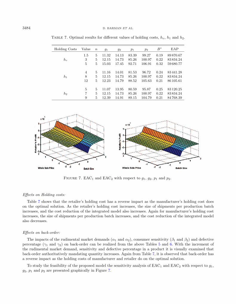
3484 D. BARMAN ET AL.
Table 7. Optimal results for different values of holding costs, ℎ𝑣, ℎ1 and ℎ2.
Holding Costs Value 𝑛 𝑔1 𝑔2 𝑝1 𝑝2 𝐵* EAP
1.5 5 11.32 14.13 83.39 99.27 0.19 89 870.67ℎ𝑣 3 5 12.15 14.73 85.26 100.97 0.22 83 834.24
5 5 15.03 17.45 92.71 106.91 0.32 59 680.77
4 5 11.16 14.01 81.53 96.72 0.24 83 441.28ℎ1 8 5 12.15 14.73 85.26 100.97 0.22 83 834.24
12 5 12.23 14.79 88.52 105.63 0.21 86 105.61
5 5 11.07 13.95 80.59 95.87 0.25 83 120.25ℎ2 7 5 12.15 14.73 85.26 100.97 0.22 83 834.24
9 5 12.39 14.91 89.15 104.79 0.21 84 768.39
Figure 7. EAC1 and EAC2 with respect to 𝑔1, 𝑔2, 𝑝1 and 𝑝2.
Effects on Holding costs:
Table 7 shows that the retailer’s holding cost has a reverse impact as the manufacturer’s holding cost doeson the optimal solution. As the retailer’s holding cost increases, the size of shipments per production batchincreases, and the cost reduction of the integrated model also increases. Again for manufacturer’s holding costincreases, the size of shipments per production batch increases, and the cost reduction of the integrated modelalso decreases.
Effects on back-order:
The impacts of the rudimental market demands (𝛼1 and 𝛼2), consumer sensitivity (𝛽1 and 𝛽2) and defectivepercentage (𝛾1 and 𝛾2) on back-order can be realized from the above Tables 5 and 6. With the increment ofthe rudimental market demand, sensitivity and defective percentage in a product it is visually examined thatback-order authoritatively mandating quantity increases. Again from Table 7, it is observed that back-order hasa reverse impact as the holding costs of manufacturer and retailer do on the optimal solution.
To study the feasibility of the proposed model the sensitivity analysis of EAC1 and EAC2 with respect to 𝑔1,𝑔2, 𝑝1 and 𝑝2 are presented graphically in Figure 7.

INTEGRATED RETAILER-MANUFACTURER MODEL FOR IMPERFECT QUALITY OF ITEMS 3485
9. Discussion
It can be observed from Tables 3 and 4 that the centralized model results more profit level than the decen-tralized model. In our proposed model, we assume that, the customer demand is linearly dependent on its retailprice. In the centralized decision making scenario, the manufacturer and all the retailers acts as a single businessmanager and jointly make their optimal decisions in order to achieve highest system profit. So, the retailers canprovide the product to the customers at a cheaper price than that of the decentralized case. That’s why lowerpriced product increases the consumer demand significantly. Then the retailers order more quantity from themanufacturer. As a result, integration between the manufacturer and all the retailers increase the total systemprofit significantly. Moreover, the retail prices of the product also decrease for both the retailers. This resultsin an increase of profit for the entire supply chain system.
10. Practical implementation and future research
This model single manufacturer multi retailer inventory model with imperfect quality of items is useful inreal life scenarios in the private, public as well as government sectors. A manufacturer may supply his/herproduct to different retailers to fulfil their requirements. For example, in health care industries, the vendorsupplies instruments to different hospitals according to their requirements. Let a health care industry namedCipla decide to distribute health care instruments like medicine, syringe, etc. among unwell people admitted indifferent hospitals and nursing home in various cities like Tamluk, Contai, Haldia, Minapore, Kharagpur, etc.in both East and West Midnapore, West Bengal. So Cipla, a private agency settle different retailers in abovesaid cities to distribute medical commodities in different hospitals and nursing homes of those cities namelyTamluk, Contai, Haldia, Midnapore, Kharagpur, etc. of both East and West Midnapore District, West Bengal.Mr. Susmit Saha a retailer in Contai has fair price shopes in different locations at Contai, Ramnagar, Digha.He can distribute medical equipment to different hospitals and nursing homes of those places through variouspaths. Like S. Saha, other retailers from different cities place the total order quantity 𝑄. Then the manufacturerproduces the total order quantity
∑𝑁𝑖=1 𝑄𝑖 of all retailers in one set up at a constant production rate 𝑅, and then
transfers the ordered quantities to the 𝑖th retailer, in 𝑛 equal batches of size 𝑔𝑖. An arriving lot may contain somedefective items. We assume that the number of defective items, 𝛿𝑖, in an arriving order of size 𝑔𝑖. Upon the arrivalof the order, A 100% screening process of the lot is conducted at the retailer’s place. Hence defective items ineach lot are discovered and returned to the manufacturer at the time of delivery of the next lot. Here, we see thatit is a very helpful easier and scientific way that, medical commodities are distributed among right people in theright way. Hence admitted people in the various nursing home and hospitals get essential services and treatedwell. Here demand is price sensitive. If the price is low, then the market demand is more; on the other hand, if theprice is high then the market demand of the product is less. Shortages are allowed and assumed to be completelybacklogged at each retailer’s end. Thus, the present investigation will be helpful to implement the above real-lifephenomena.
In our proposed model, we have considered that one manufacturer is trading with multiple retailers for a singleproduct. Our model can be further extended considering multiple items. One can also implement any suitablecoordination scheme between the manufacturer and all the retailers to improve their profits in the decentralizedscenario. Furthermore, our proposed model can be enriched by considering more realistic assumptions, suchas combined equal and unequal sized batch shipments, quality dependent demand and multiple manufacturerstrading with multiple retailers. Also, The formulate models have great opportunity to extend with breakableitems, imperfect production and for another type stochastic distributions. The model can be formulated withfuzzy, fuzzy-rough and fuzzy-random coefficients. Moreover, the model can be solved by using other type ofoptimisation techniques.

3486 D. BARMAN ET AL.
11. Conclusion with managerial implications and insight
In this paper, we have considered a two-level supply chain model consisting of a single manufacturer andmultiple retailers under price sensitive customer demand and stochastic lead time. The manufacturer producesa single product at a constant production rate and transfers it to the retailers in some equal batch shipments.An arriving lot may contain some defective items (Which is random in nature) 𝛿𝑖, in an order of size 𝑔𝑖. Onthe arrival of order, A 100% screening process of the lot is conducted at the retailer’s place. Hence defectiveitems which incur a warranty cost of 𝜈 for the manufacturer in each lot are discovered and returned to themanufacturer. The manufacturer will sell the defective items at a reduced price to other retailer or recycle itfor delivery of the next lot. Due to the stochastic nature of lead time the batches may reach early or late to theretailers. Depending on the length of lead time duration, all three possible cases are taken into considerationat the retailers end. Decentralized and centralized models are formulated. A solution algorithm is derived tofind the optimal solutions in the decentralized model with a Stackelberg gaming structure. It is found thatcooperation between the manufacturer and the retailers becomes more profitable for the entire supply chainwhenever the consumer demand is price dependent and lead time of delivering the ordered quantity follows anormal distribution. By collaborating with each other, the supply chain players can sell the product at a cheaperprice to the end customers and enhance market demand. This leads to a significant increment of the profitabilityof the whole supply chain.
Supply chain management is an integral part in most of the business system and essential company successthrough boosting of customer services, reducing of operating costs, improving of financial position. It alsoensures sustain of human life, protection of climate extremes, improve the economic growth as well as benefitof customers. In developing countries, like India, Bangladesh, Nepal, China, etc., due to several reasons, manyparameters like demand, lead time, quality assurance, etc. seemed uncertain in nature. In recent time vastgrowth of population compel companies to makes huge production to fulfil population demand. So, the sellingprice plays an important role in determining the inventory or supply chain strategies. For these reasons, if wecollect the previous data from any management system belong to these countries and followed by statisticalregularity criteria, its probability distribution can be obtained for future correspondence In this paper a focuson the study an integrated single manufacturer multi retailer model for imperfect quality of items having price-dependent market demand determines the optimal decisions which maximize the joint total profit of the wholesupply chain.
Appendix A.
Implementing GAA typical Genetic Algorithm requires the following stages.
(i) ParametersFirstly, we set the values of different parameters on which this GA depends, like number of generations(MAXGEN), population size (POPSIZE), probability of crossover (PXOVER), and probability of mutation(PMU).(ii) Chromosome representationAn important issue of a GA is to design appropriate chromosomes for the representation of solutions of theproblem together with genetic operators. Since the proposed problem is highly non-linear, to overcome thisdifficulty the chromosomes are repeated by real-numbers. In this representation, each chromosome 𝑋𝑝 is astring of genes 𝐺𝑝, where genes 𝐺𝑝 denote the decision variables 𝑚 and 𝑇1 of the model. Since real-numberrepresentation is used here, the value of each chromosome is the actual value of the decision variable.(iii) Initial population productionWe first determine the independent and dependent variables and then their boundaries. All genes correspondingto all the independent variables are generated randomly between its boundaries and dependent variables are
INTEGRATED RETAILER-MANUFACTURER MODEL FOR IMPERFECT QUALITY OF ITEMS 3487
generated by using different conditions.(iv) EvaluationThe evaluation of function plays the same role in the GA as that which the environment plays in naturalevolution. For this problem, the evaluation function is EVAL(𝐺𝑝) = value of objective function 𝐴𝐶(𝑇1, 𝑚).(v) SelectionThe selection scheme of GA determines which chromosomes in the current population are to be selected fornext generation. There are several approaches to select chromosomes from the initial population for theirmating pool. All these approaches have some merits and demerits over the others. Among these approachesRoulette wheel selection process is very popular. In this study, Roulette wheel selection process is used withthe following steps
(a) Find total fitness of the population
𝐹 =POPSIZE∑
𝑝=1
𝑍(𝐺𝑝)
(b) Calculate the probability of selection 𝑃sel of each solution 𝐺𝑝 by the formula
𝑃sel(𝐺𝑝) =𝑍(𝐺𝑝)
𝐹
(c) Calculate the cumulative probability 𝑃 ′sel(𝐺𝑝) for each solution 𝐺𝑝 by the formula
𝑃 ′sel(𝐺𝑝) =𝑝∑
𝑘=1
𝑃sel(𝐺𝑘)
(d) Generate a random number 𝑟 from the range [0, 1].(e) If 𝑟 < 𝑃 ′sel(1) then select 𝐺1 otherwise select 𝐺𝑝(2 ≤ 𝑝 ≤ POPSIZE) if 𝑃 ′sel(𝐺𝑝−1) ≤ 𝑟 < 𝑃 ′sel(𝐺𝑝).(f) Repeat steps (iv) and (v) POPSIZE times to select the chromosomes for mating pool. These chromosomes
are denoted by 𝐺𝑁𝑗 , 𝑗 = 1, 2, ....., POPSIZE. Clearly one chromosome may be selected more than once andso some members of this set may be identical.
(g) Selected chromosomes set is denoted by 𝑇 = 𝐺𝑁1, 𝐺𝑁2, ...., 𝐺𝑁POPSIZE in the proposed GA algorithm.
(vi) CrossoverCrossover is a key operator in the GA and is used to exchange the main characteristics of parent individualsand pass them to the children. it consists of two steps:
(a) Selection for crossover: For each solution of 𝑃 1(𝑇 ) generate a random number 𝑟 from the range [0, 1]. If𝑟 < 𝑝𝑐 then the solution is taken for the crossover. Where 𝑝𝑐 is the probability of the crossover.
(b) Crossover process: Crossover taken place on the selected solutions. for pair coupled solution 𝑀1, 𝑀2 arandom number 𝑐 is generated from the range [0, 1] and 𝑀1, 𝑀2 are replaced by their offsprings 𝐺1, 𝐺2
respectively. where 𝐺1 = 𝑐1𝑀1+(1−𝑐)𝑀2,𝐺2 = (1−𝑐)𝑀1+𝑐1𝑀2, provided 𝐺1, 𝐺2 satisfied the constraintsof the problem.
(vii) MutationAs in the conventional GA scheme, a parameter 𝑃𝑚 of the genetic system is defined as the probability ofmutation. The mutation operation is performed on a bit-by-bit basis, where for a random number 𝑟 ∈ [0, 1], achromosome is selected for mutation provided that 𝑟 < 𝑃𝑚.(viii) ImplementationWith the above function and values the algorithm is implemented using C-programming language.(ix) TerminationIf number of iterations is less than to MAXGEN then the process continues, otherwise it terminates. Therefore,

3488 D. BARMAN ET AL.
in this study at the end of last generation, each individual in the last generation is studied to check there isany local optimal in their neighborhoods. To do this, all the neighbor solutions to each individual are searchedand evaluated successfully.
Appendix B.
The profit function can be computed as:
EAP(𝑛, 𝑔𝑖, 𝑝𝑖) =𝑁∑
𝑖=1
𝐷𝑖(𝑝𝑖 − 𝑑𝑖)(1− 𝛾𝑖)
− 𝑆𝑣
𝑁∑𝑖=1
𝐷𝑖
𝑛𝑔𝑖(1− 𝛾𝑖)− 𝜈
𝑁∑𝑖=1
𝛾𝑖𝐷𝑖
(1− 𝛾𝑖)− ℎ𝑣
[ 𝑁∑𝑖=1
𝑔𝑖
𝑅
𝑁∑𝑖=1
𝐷𝑖
(1− 𝛾𝑖)
+𝑄
2
{1− 𝐷
𝑅
𝑁∑𝑖=1
1(1− 𝛾𝑖)
}−
𝑁∑𝑖=1
𝑔𝑖
2𝑛(1− 𝛾𝑖)
]− ℎ𝑣
𝑁∑𝑖=1
1− 𝑔𝑖𝛾𝑖
1− 𝛾𝑖
{𝐷𝑖𝐼6
−𝑟𝑖(1− 𝐹 (𝑟𝑖
𝐷𝑖))
}−
𝑁∑𝑖=1
[𝐷𝑖
𝑛𝑔𝑖(1− 𝛾𝑖)(𝐴𝑖 + 𝑛𝑇𝑝) +
ℎ𝑖
1− 𝛾𝑖
{𝑟𝑖(1− 𝑔𝑖𝛾𝑖)
+𝐷𝑖𝑔
2𝑖 𝛾𝑖
𝑧𝑖+
𝑔𝑖
2(1− 𝑔𝑖𝛾𝑖 − 𝑔𝑖𝛾
2𝑖 + 𝑔2
𝑖 𝛾2𝑖 )
}𝐹 (
𝑟𝑖
𝐷𝑖)− ℎ𝑖
1− 𝛾𝑖
{𝐷𝑖
2𝑔𝑖+ (1− 𝑔𝑖𝛾𝑖)𝐷𝑖
}𝐼1
+ℎ𝑖
1− 𝛾𝑖
𝐷2𝑖
2𝑔𝑖𝐼2 +
ℎ𝑖
1− 𝛾𝑖
{𝑟2𝑖
3𝑔𝑖+
𝐷𝑖𝑔2𝑖 𝛾𝑖
𝑧𝑖+ 𝑟𝑖(1− 𝑔𝑖𝛾𝑖)−
𝐷𝑖𝑟𝑖
2𝑧𝑖𝐴1𝑖
+12
(𝑔𝑖(1− 𝑔𝑖𝛾𝑖 − 𝑔𝑖𝛾2𝑖 + 𝑔2
𝑖 𝛾2𝑖 ) + 𝑟𝑖𝐴2𝑖) + 𝑟𝑖(1− 𝑔𝑖𝛾𝑖) +
𝑟2𝑖
𝑔𝑖𝐴1𝑖
}𝐼3 −
ℎ𝑖
1− 𝛾𝑖
{𝐷𝑖
𝑔𝑖
−𝐷2𝑖
2𝑧𝑖𝐴1𝑖 + 𝐷𝑖𝐴2𝑖 + 𝐷𝑖(1− 𝑔𝑖𝛾𝑖) +
2𝐷𝑖𝑟𝑖
𝑔𝑖𝐴1𝑖
}𝐼4 +
ℎ𝑖𝐷𝑖
𝑔𝑖(1− 𝛾𝑖)𝐼5
+𝑏𝑖
2𝑔𝑖(1− 𝛾𝑖)
{1 +
𝐷𝑖
𝑧𝑖𝐴3𝑖
}(𝐷2
𝑖 𝐼5 − 2𝐷𝑖𝑟𝑖𝐼4 + 𝑟2𝑖 𝐼3
)+
𝑐𝑖
1− 𝛾𝑖{𝐷𝑖𝐼7 − (𝑟𝑖 +
𝑔2𝑖
2)(1− 𝐹 (
(𝑟𝑖 + 𝑔𝑖)𝐷𝑖
))}],
where
𝐴1𝑖 = 𝐸
[(1− 𝛿𝑖)
(1− 𝛿𝑖 − 𝐷𝑖
𝑧𝑖)
]=
(1− 𝑔𝑖𝛾𝑖)(1− 𝑔𝑖𝛾𝑖 − 𝐷𝑖
𝑧𝑖),
𝐴2𝑖 = 𝐸
[(1− 𝛿2
𝑖 )(1− 𝛿𝑖 − 𝐷𝑖
𝑧𝑖)
]=
(1− 𝑔𝑖𝛾𝑖 − 𝑔𝑖𝛾2𝑖 + 𝑔2
𝑖 𝛾2𝑖 )
(1− 𝑔𝑖𝛾𝑖 − 𝐷𝑖
𝑧𝑖)
,
𝐴3𝑖 = 𝐸
[1
(1− 𝛿𝑖 − 𝐷𝑖
𝑧𝑖)
]=
1(1− 𝑔𝑖𝛾𝑖 − 𝐷𝑖
𝑧𝑖).
Appendix C.
When 𝑙𝑖 is exponentially distributed with 𝑝.𝑑.𝑓. 𝑓(𝑙𝑖) = 𝜆𝑖𝑒−𝜆𝑖𝑙𝑖 , the expression of 𝐹 ( 𝑟𝑖
𝐷𝑖) as well as 1−𝐹 ( 𝑟𝑖
𝐷𝑖),
𝐹 ( 𝑟𝑖+𝑔𝑖
𝐷𝑖), 1− 𝐹 ( 𝑟𝑖+𝑔𝑖
𝐷𝑖) 𝐼1, 𝐼2, 𝐼3, 𝐼4, 𝐼5, 𝐼6, 𝐼7 are the following:
𝐹 (𝑟𝑖
𝐷𝑖) =
∫ 𝑟𝑖𝐷𝑖
0
𝑓(𝑙𝑖)d𝑙𝑖 =∫ 𝑟𝑖
𝐷𝑖
0
𝜆𝑖𝑒−𝜆𝑖𝑙𝑖d𝑙𝑖 = 1− 𝑒
−𝜆𝑖𝑟𝑖𝐷𝑖 ,

INTEGRATED RETAILER-MANUFACTURER MODEL FOR IMPERFECT QUALITY OF ITEMS 3489
and 𝐹 (𝑟𝑖 + 𝑔𝑖
𝐷𝑖) =
∫ 𝑟𝑖+𝑔𝑖𝐷𝑖
0
𝑓(𝑙𝑖)d𝑙𝑖 =∫ 𝑟𝑖+𝑔𝑖
𝐷𝑖
0
𝜆𝑖𝑒−𝜆𝑖𝑙𝑖d𝑙𝑖 = 1− 𝑒
−𝜆𝑖(𝑟𝑖+𝑔𝑖)𝐷𝑖 .
Hence, 1− 𝐹 (𝑟𝑖
𝐷𝑖) = 𝑒
−𝜆𝑖𝑟𝑖𝐷𝑖 ,
1− 𝐹 (𝑟𝑖 + 𝑔𝑖
𝐷𝑖) = 𝑒
−𝜆𝑖(𝑟𝑖+𝑔𝑖)𝐷𝑖 .
Similarly,
𝐼1 =∫ 𝑟𝑖
𝐷𝑖
0
𝑙𝑖𝑓(𝑙𝑖)d𝑙𝑖 =∫ 𝑟𝑖
𝐷𝑖
0
𝑙𝑖𝜆𝑖𝑒−𝜆𝑖𝑙𝑖d𝑙𝑖 =
1𝜆𝑖− (
1𝜆𝑖
+𝑟𝑖
𝐷𝑖)𝑒−𝜆𝑖𝑟𝑖
𝐷𝑖 ,
𝐼2 =∫ 𝑟𝑖
𝐷𝑖
0
𝑙2𝑖 𝑓(𝑙𝑖)d𝑙𝑖 =∫ 𝑟𝑖
𝐷𝑖
0
𝑙2𝑖 𝜆𝑖𝑒−𝜆𝑖𝑙𝑖d𝑙𝑖 =
2𝜆2
𝑖
− { 1𝜆2
𝑖
+ (1𝜆𝑖
+𝑟𝑖
𝐷𝑖)2}𝑒
−𝜆𝑖𝑟𝑖𝐷𝑖 ,
𝐼3 =∫ 𝑟𝑖+𝑔𝑖
𝐷𝑖
𝑟𝑖𝐷𝑖
𝑓(𝑙𝑖)d𝑙𝑖 =∫ 𝑟𝑖+𝑔𝑖
𝐷𝑖
𝑟𝑖𝐷𝑖
𝜆𝑖𝑒−𝜆𝑖𝑙𝑖d𝑙𝑖 = 𝑒
−𝜆𝑖𝑟𝑖𝐷𝑖 − 𝑒
−𝜆𝑖(𝑟𝑖+𝑔𝑖)𝐷𝑖 ,
𝐼4 =∫ 𝑟𝑖+𝑔𝑖
𝐷𝑖
𝑟𝑖𝐷𝑖
𝑙𝑖𝑓(𝑙𝑖)d𝑙𝑖 =∫ 𝑟𝑖+𝑔𝑖
𝐷𝑖
𝑟𝑖𝐷𝑖
𝑙𝑖𝜆𝑖𝑒−𝜆𝑖𝑙𝑖d𝑙𝑖 = (
1𝜆𝑖
+𝑟𝑖
𝐷𝑖)𝑒−𝜆𝑖𝑟𝑖
𝐷𝑖 − (1𝜆𝑖
+(𝑟𝑖 + 𝑔𝑖)
𝐷𝑖)𝑒−𝜆𝑖(𝑟𝑖+𝑔𝑖)
𝐷𝑖 ,
𝐼5 =∫ 𝑟𝑖+𝑔𝑖
𝐷𝑖
𝑟𝑖𝐷𝑖
𝑙2𝑖 𝑓(𝑙𝑖)d𝑙𝑖 =∫ 𝑟𝑖+𝑔𝑖
𝐷𝑖
𝑟𝑖𝐷𝑖
𝑙2𝑖 𝜆𝑖𝑒−𝜆𝑖𝑙𝑖d𝑙𝑖
=1𝜆2
𝑖
{1 +1
𝐷2𝑖
(𝐷𝑖 + 𝜆𝑖𝑟𝑖)2}𝑒−𝜆𝑖𝑟𝑖
𝐷𝑖 − 1𝜆2
𝑖
[1 +1
𝐷2𝑖
{𝐷𝑖 + 𝜆𝑖(𝑟𝑖 + 𝑔𝑖)}2]𝑒−𝜆𝑖(𝑟𝑖+𝑔𝑖)
𝐷𝑖 ,
𝐼6 =∫ ∞
𝑟𝑖𝐷𝑖
𝑙𝑖𝑓(𝑙𝑖)d𝑙𝑖 =∫ ∞
𝑟𝑖𝐷𝑖
𝑙𝑖𝜆𝑖𝑒−𝜆𝑖𝑙𝑖d𝑙𝑖 = (
1𝜆𝑖
+𝑟𝑖
𝐷𝑖)𝑒−𝜆𝑖𝑟𝑖
𝐷𝑖 ,
𝐼7 =∫ ∞
(𝑟𝑖+𝑔𝑖)𝐷𝑖
𝑙𝑖𝑓(𝑙𝑖)d𝑙𝑖 =∫ ∞
(𝑟𝑖+𝑔𝑖)𝐷𝑖
𝑙𝑖𝜆𝑖𝑒−𝜆𝑖𝑙𝑖d𝑙𝑖 = { 1
𝜆𝑖+
(𝑟𝑖 + 𝑔𝑖)𝐷𝑖
}𝑒−𝜆𝑖𝑟𝑖
𝐷𝑖 .
Acknowledgements. The authors are grateful to the associate editor and anonymous reviewers for their valuable commentsand suggestions to improve the quality of this article.
References
[1] H.K. Alfares and A.M. Ghaithan, Inventory and pricing model with price-dependent demand, time-varying holding cost, andquantity discounts. Comput. Ind. Eng. 94 (2016) 170–177.
[2] A. Banarjee, A joint economic-lot-size model for purchaser and vendor. Decision Sci. 17 (1986) 292–311.
[3] D. Barman and B. Das, An imprecise-inventory model with PEND and SEND policy. Int. J. Math. Oper. Res. 13 (2018)243–268.
[4] D. Barman and B. Das, Two-echelon supply chain inventory model with variable lead time and ramp-type demand for deteri-oration item under bi-level credit period. IJIR 6 (2021) 14–46.
[5] D. Barman, G.C. Mahata and B. Das, Advance payment based vendor-buyer production inventory model with stochastic leadtime and continuous review policy. Opsearch 58 (2021) 1217–1237.
[6] H. Barman, M. Pervin, S.K. Roy and G.W. Weber, Back-ordered inventory model with inflation in a Cloudy-Fuzzy environment.J. Ind. Manag. Optim. 17 (2021) 1913–1941.
[7] M. Ben-Daya and M. Hariga, Integrated single vendor single buyer model with stochastic demand and variable lead time. Int.J. Prod. Econ. 92 (2004) 75–80.
[8] J. Bhowmick and G.P. Samanta, Optimal inventory policies for imperfect inventor with price dependent stochastic demandand partially backlogged shortages. Yugosl. J. Oper. Res. 22 (2012) 199–223.
[9] L.E. Cardenas-Barron, Economic production quantity with rework process at a single-stage manufacturing system with plannedback-orders. Comput. Ind. Eng. 57 (2009) 1105–1113.

3490 D. BARMAN ET AL.
[10] B.K. Dey, B. Sarkar, M. Sarkar and S. Pareek, An integrated inventory model involving discrete setup cost reduction, variablesafety factor, selling price dependent demand, and investment. RAIRO-Oper. Res. 53 (2019) 39–57.
[11] A. Gholami and A. Mirzazadeh, An inventory model with controllable lead time and ordering cost, log-normal-distributeddemand, and gamma-distributed available capacity. Cogent Bus. Manag. 5 (2018) 1469182.
[12] B.C. Giri and M. Masanta, Optimal production policy for a closed-loop supply chain with stochastic lead time and learningin production. Scientia Iranica 26 (2019) 2936–2951.
[13] B.C. Giri and M. Masanta, Developing a closed-loop supply chain model with price and quality dependent demand and learningin production in a stochastic environment. Int. J. Syst. Sci. Oper. Logist. 7 (2020) 147–163.
[14] D. Goldberg, Genetic algorithms in search, optimization, and machine learning. Addison-Wesley, Reading, MA (1989).
[15] S.K. Goyal, An integrated inventory model for a single supplier-single customer problem. Int. J. Prod. Res. 15 (1976) 107–111.
[16] F.W. Harris, How many parts to make at once. Mag. Manage. 10(2) (1913) 135–136, 152. [Reprinted in Oper. Res. 38 (1990)947–950.
[17] M.A. Hoque, A manufacturer-buyer integrated inventory model with stochastic lead times for delivering equal-and/or unequal-sized batches of a lot. Comput. Oper. Res. 40 (2013) 2740–2751.
[18] J.T. Hsu and L.F. Hsu, An integrated vendor-buyer inventory model with imperfect items and planned back orders. Int. J.Adv. Manuf. Technol. 68 (2013) 2121–2132.
[19] C.K. Jaggi, Rini and A. Kishore, Replenishment policies for imperfect inventory system under natural idle time and shortages.Yugosl. J. Oper. Res. 30 (2020) 251–270.
[20] J.K. Jha and K. Shanker, Single-vendor multi-buyer integrated production-inventory model with controllable lead time andservice level constraints. Appl. Math. Model. 37 (2013) 1753–1767.
[21] P. Jindala and A. Solanki, Integrated vendor-buyer inventory models with inflation and time value of money in controllablelead time. Decision Sci. Lett. 5 (2016) 81–94.
[22] N. Kazemi, S.H. Abdul-Rashid, R.A. Ghazilla, E. Shekarian and S. Zanoni, Economic order quantity models for items withimperfect quality and emission considerations. Int. J. Syst. Sci. Oper. Logist. 5 (2018) 99–115.
[23] A. Khanna, A. Kishore, B. Sarkar and C.K. Jaggi, Inventory and pricing decisions for imperfect quality items with inspectionerrors, sales returns, and partial back-orders under inflation. RAIRO-Oper. Res. 54 (2020) 287–306.
[24] A. Kocabiyikoglu and I. Popescu, An elasticity approach to the news vendor with price-sensitive demand. Oper. Res. 59 (2011)301–312.
[25] Y. Li, X. Xu and F. Ye, Supply chain coordination model with controllable lead time and service level constraint. Comput.Indus. Eng. 61 (2011) 858–864.
[26] H.J. Lin, An integrated supply chain inventory model with imperfect-quality items, controllable lead time and distribution freedemand. Yugosl. J. Oper. Res. 23 (2013) 87–109.
[27] H.J. Lin, Investing in lead-time variability reduction in a collaborative vendor-buyer supply chain model with stochastic leadtime. Comput. Oper. Res. 72 (2016) 43–49.
[28] C. Mahato, S.K. De and G.C. Mahata, Joint pricing and inventory management for growing items in a supply chain undertrade credit. Soft. Comput. 25 (2021) 7271–7295.
[29] M.K. Maiti, A fuzzy genetic algorithm with varying population size to solve an inventory model with credit-linked promotionaldemand in an imprecise planning horizon. Eur. J. Oper. Res. 213 (2011) 96–106.
[30] P. Mandal and B.C. Giri, A single-vendor multi-buyer integrated model with controllable lead time and quality improvementthrough reduction in defective items. Int. J. Syst. Sci. Oper. Logist. 2 (2015) 1–14.
[31] L.Y. Ouyang, K.S. Wu and C.H. Ho, Integrated vendor-buyer cooperative models with stochastic demand in controllable leadtime. Int. J. Prod. Econ. 92 (2004) 255–266.
[32] A. Paul, M. Pervin, S.K. Roy, G.W. Weber and A. Mirzazadeh, Effect of price-sensitive demand and default risk on optimalcredit period and cycle time for a deteriorating inventory model. RAIRO-Oper. Res. 55 (2021) S2575–S2592.
[33] M. Pervin, S.K. Roy and G.W. Weber, Deteriorating inventory with preservation technology under price- and stock-sensitivedemand. J. Indus. Manage. Optim. 16 (2020) 1585–1612.
[34] M. Pervin, S.K. Roy and G.W. Weber, An integrated vendor-buyer model with quadratic demand under inspection policy andpreservation technology. Hacettepe J. Math. Stat. 49 (2020) 1168–1189.
[35] T. Poorbagheri and S.T.A. Niaki, Vendor Managed inventory of a single-vendor multiple-retailer single-warehouse SupplyChain under stochastic Demands. Int. J. Supply Oper. Manage. 1 (2014) 297–313.
[36] E.L. Porteus, Optimal lot sizing, process quality improvement and setup cost reduction. Oper. Res. 34 (1986) 37–144.
[37] S. Ray and E.M. Jewkes, Customer lead time management when both demand and price are lead time sensitive. Eur. J. Oper.Res. 153 (2004) 769–781.
[38] W. Ritha and S. Poongodisathiya, Multiple-buyer single-vendor in a continuous review inventory model with ordering costreduction dependent on lead time. Int. J. Recent Innov. Trends Comput. Communi. 6 (2018) 154–160.
[39] M.J. Rosenblatt and H.L. Lee, Economic production cycles with imperfect production processes. IIE Trans. 18 (1986) 48–55.
[40] M.K. Salameh and M.Y. Jaber, Economic production quantity model for items with imperfect quality. Int. J. Prod. Econ. 64(2000) 59–64.
[41] S. Sarkar, S. Tiwari, H.M. Wee and B.C. Giri, Channel coordination with price discount mechanism under price-sensitivemarket demand. Int. Trans. Oper. Res. 27 (2019) 1–25.
[42] M.S. Sohrabi, P. Fattahi, A.S. Kheirkhah and G. Esmaeilian, Supplier selection in three echelon supply chain and vendormanaged inventory model under price dependent demand condition. Int. J. Supply Oper. Manage. 2 (2016) 1079–1101.
INTEGRATED RETAILER-MANUFACTURER MODEL FOR IMPERFECT QUALITY OF ITEMS 3491
[43] M. Taghizadeh-Yazdi, Z. Farrokhi and A. Mohammadi-Balani, An integrated inventory model for multi-echelon supply chainswith deteriorating items: a price-dependent demand approach. J. Indus. Prod. Eng. 37 (2020) 87–96.
[44] A.A. Taleizadeh, A constrained integrated imperfect manufacturing-inventory system with preventive maintenance and partialbackordering. Ann. Oper. Res. 261 (2018) 303–337.
[45] A.A. Taleizadeh, M.P.S. Khanbaglo and L.E. Cardenas-Barron, An EOQ inventory model with partial backordering andreparation of imperfect products. Int. J. Prod. Econ. 182 (2016) 418–434.
[46] A.A. Taleizadeh, S.T.A. Niaki and A.Makui, Multiproduct multiple-buyer single-vendor supply chain problem with stochasticdemand, variable lead-time, and multi-chance constraint. Expert Syst. Appl. 39 (2012) 5338–5348.
[47] R. Uthayakumar and M.G. Kumar. Single-vendor multi-buyer integrated inventory system for multi-item. Int. J. Math. Oper.Res 14 (2019) 359–376.
[48] I.D. Wangsa and H.M. Wee, A vendor-buyer inventory model for defective items with errors in inspections, stochastic leadtime and freight cost. INFOR 57 (2019) 597–622.
[49] T.M. Whitin, Inventory control and price theory. Manage. Sci. 2 (1955) 61–68.
[50] P.C. Yang, S.L. Chung, H.M. Wee, E. Zahara and C.Y. Peng, Collaboration for a closed-loop deteriorating inventory supplychain with multi-retailer and price-sensitive demand. Int. J. Prod. Econ. 143 (2013) 557–566.
[51] B. Yang and J. Geunes, Inventory and lead time planning with lead-time sensitive demand. IIE Trans. 39 (2007) 439–452.
This journal is currently published in open access under a Subscribe-to-Open model (S2O). S2O is a transformativemodel that aims to move subscription journals to open access. Open access is the free, immediate, online availability ofresearch articles combined with the rights to use these articles fully in the digital environment. We are thankful to oursubscribers and sponsors for making it possible to publish this journal in open access, free of charge for authors.
Please help to maintain this journal in open access!
Check that your library subscribes to the journal, or make a personal donation to the S2O programme, by [email protected]
More information, including a list of sponsors and a financial transparency report, available at: https://www.edpsciences.org/en/maths-s2o-programme