A Simulation Testbed for Airborne Merging and Spacing · spacing = duration of time-based spacing...

A Simulation Testbed forAirborne Merging and Spacing

Michel Santos*, Vikram Manikonda†, Art Feinberg‡

Intelligent Automation, Inc.Rockville, Maryland, USA

Gary Lohr§

National Aeronautics and Space Administration Langley Research CenterHampton, Virginia, USA

The key innovation in this effort is the development of a simulation testbed for airborne merging and spacing (AM&S). We focus on concepts related to airports with Super Dense Operations where new airport runway configurations (e.g. parallel runways), sequencing, merging, and spacing are some of the concepts considered. We focus on modeling and simulating a complementary airborne and ground system for AM&S to increase efficiency and capacity of these high density terminal areas. From a ground systems perspective, a scheduling decision support tool generates arrival sequences and spacing requirements that are fed to the AM&S system operating on the flight deck. We enhanced NASA's Airspace Concept Evaluation Systems (ACES) software to model and simulate AM&S concepts and algorithms.

NomenclatureACES = Airspace Concept Evaluation System

AM&S = airborne merging and spacing

ft. = feet

IAS = indicated airspeed

n.mi. = nautical mile

NAS = national airspace system

STA = scheduled time of arrival

t spacing = duration of time-based spacing between aircraft

I. IntroductionAir traffic demand over the next few years is expected to increase significantly with demand in 2025 reaching

almost three times current demand1. Traffic management flow efficiency, airport and terminal throughput and controller workload remain some of the foremost limitations of the air traffic system. To address this issue the Joint Planning and Development Office (JPDO) is currently working to define the Next Generation Air Transportation System (NGATS) with the objective of determining what changes are necessary to meet future demand. NASA’s NGATS ATM-Airportal project currently supports this vision by focusing research efforts to develop, demonstrate, and validate operational concepts, proof-of-concept systems, algorithms, technologies, tools, and operational procedures for use in maximizing capacity and throughput in the Airportal environment.

*Research Scientist, Intelligent Automation, 15400 Calhoun Drive, Suite 400, Rockville, MD 20855, AIAA Member†Vice President, Intelligent Automation, 15400 Calhoun Drive, Suite 400, Rockville, MD 20855, AIAA Member‡Program Manager, Intelligent Automation, 15400 Calhoun Drive, Suite 400, Rockville, MD 20855§Aerospace Technologist, NASA Langley Research Center, M/S 156A, Hampton, VA 23681

1American Institute of Aeronautics and Astronautics

https://ntrs.nasa.gov/search.jsp?R=20080034651 2020-05-28T10:09:25+00:00Z

This research effort directly supports the objectives of the NASA Airportal Project. AM&S is envisioned as one of the key concepts that will result in achieving increased efficiency in the Airportal environment. This effort has resulted in the development of an operational concept, modeling and simulation capability that will enable the evaluation of technologies related to AM&S. As discussed in the Federal Aviation Administration (FAA)/JPDO Industry Day Briefing on Surveillance and Broadcast Services¶, with the equipage of all aircraft with Automatic Dependent Surveillance Broadcast (ADS-B), it is anticipated that significant capacity and safety gains will be realized by the delegation of responsibilities related to self-separation, merging, and spacing to the flight deck. Some examples of expected operational improvements include:

• Reduced arrival spacing (with altitude offset) for very closely spaced parallel runways at Operational Evaluation Plan (OEP) airports (Super Dense Airports Concepts) • High density en route corridors (tubes) characterized by parallel tracks and delegation of separation responsibility to the flight deck via CDTI and ADS-B• Self-spacing with CDTI/ADS-B coupled with sequencing automation use at non-towered airports

Airborne separation and assurance systems (ASAS) are being researched under the guiding principle that “Air Traffic Services can be enhanced through greater involvement of flight crews and aircraft systems in cooperation with controllers and the Air Traffic Management system.”2 Section II briefly surveys the research on ASAS which includes research on AM&S. Section III identifies the AM&S concepts used for this paper. Section IV reviews how the AM&S concepts are implemented within ACES3. Section V presents the results from some AM&S simulation studies within ACES.

II. Literature Survey of Airborne Separation Assurance SystemsAirborne separation and assurance systems have been categorized into four applications2: airborne traffic

situational awareness, airborne spacing applications, airborne separation applications, and airborne self-separation. Airborne traffic situational awareness is aimed at enhancing the flight crews' knowledge of the surrounding traffic situation both in the air and on the airport surface. In airborne spacing applications, the controller instructs flight crews to achieve and maintain a given spacing with designated aircraft. In airborne separation applications, the controller instructs flight crews to maintain separation from designated aircraft. In airborne self-separation applications, flight crews bear the responsibility of separating their own aircraft from all surrounding traffic.

Research on airborne traffic situational awareness has partly focused on presenting additional air traffic information to flight crews. Some information, such as the position and velocity of surrounding aircraft, can be obtained either through Automatic Dependent Surveillance - Broadcast (ADS-B)4, which is broadcast by the surrounding aircraft themselves, or through Traffic Information Service - Broadcast (TIS-B)5, which can be broadcast by radar-equipped ground stations on behalf of transponder-equipped aircraft that are incapable of broadcasting ADS-B data. Once obtained, this information can be displayed on cockpit displays of traffic information (CDTI)6. Several human factor studies related to CDTI have been undertaken by NASA7,8,9.

Airborne spacing applications have been researched from multiple perspectives. Some work has investigated in-trail spacing by using automated control laws without humans-in-the-loop. This is done partly to isolate the dynamics between spaced aircraft10,11,12 and partly to identify critical characteristics of the data link from the aircraft being followed13,14. The use of human flight crews in spacing applications has studied pilot effectiveness, workload, and trust15,16,17. Similar studies have also been undertaken from the controller perspective18,19,20. Interestingly, the controllers studied in Ref. 19 preferred issuing maneuvering instructions to flight crews rather than delegating the spacing responsibility to them.

Airborne separation has been investigated to determine whether it can increase controller availability and enhance flight crew situational. Some research has focused on the communications procedures to be used to enact controller-designated separation21,22. Controller-designated separation instructions sometimes consist of two instructions: an explicit maneuvering instruction that redirects the aircraft around another aircraft, and an instruction to resume course afterwards22,23. In another case, the separation instruction includes the aircraft to avoid yet leaves the maneuver selection to the flight deck21.

Airborne self-separation applications have previously been studied under the names of “free flight”24,25 and “distributed air/ground traffic separation and management (DAG-TM)”26,27. The issues identified have ranged from: making aircraft situationally aware through data links28; identifying conflicts based on trajectory predictions29 and/or intent information30; and resolving trajectory conflicts by independent maneuvering of individual aircraft31,32, maneuvering of pairs of aircraft through trajectory negotiations33, maneuvering of pairs of aircraft by standard maneuvers33,34, and maneuvering as instructed by controllers who exercise positive control33.

¶FAA Industry Day Briefing on Surveillance and Broadcast Service, June 19, 20062

American Institute of Aeronautics and Astronautics

This work is covered under airborne situational awareness and airborne spacing applications.

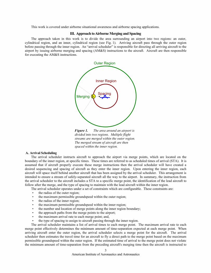
III. Approach to Airborne Merging and SpacingThe approach taken in this work is to divide the area surrounding an airport into two regions: an outer,

cylindrical region, and an inner, cylindrical region (see Fig. 1). Arriving aircraft pass through the outer region before passing through the inner region. An “arrival scheduler” is responsible for directing all arriving aircraft to the airport by issuing airborne merging and spacing (AM&S) instructions to the aircraft. Aircraft are then responsible for executing the AM&S instructions.

Outer Region

Inner Region

MergingSpacing

Figure 1. The area around an airport is divided into two regions. Multiple flight streams are merged within the outer region. The merged stream of aircraft are then spaced within the inner region.

A. Arrival SchedulingThe arrival scheduler instructs aircraft to approach the airport via merge points, which are located on the

boundary of the inner region, at specific times. These times are referred to as scheduled times of arrival (STA). It is assumed that if aircraft properly execute these merge instructions then the arrival scheduler will have created a desired sequencing and spacing of aircraft as they enter the inner region. Upon entering the inner region, each aircraft will space itself behind another aircraft that has been assigned by the arrival scheduler. This arrangement is intended to ensure a stream of safely-separated aircraft all the way to the airport. In summary, the instruction from the arrival scheduler to the aircraft includes a STA to a specific merge point, the identification of the lead aircraft to follow after the merge, and the type of spacing to maintain with the lead aircraft within the inner region.

The arrival scheduler operates under a set of constraints which are configurable. These constraints are:• the radius of the outer region;• the maximum permissible groundspeed within the outer region;• the radius of the inner region;• the maximum permissible groundspeed within the inner region;• the number and location of merge points along the inner region boundary;• the approach paths from the merge points to the airport;• the maximum arrival rate to each merge point; and,• the type of spacing to assign to aircraft passing through the inner region.

The arrival scheduler maintains a list of arrival times to each merge point. The maximum arrival rate to each merge point effectively determines the minimum amount of time-separation expected at each merge point. When arriving aircraft enter the outer region, the arrival scheduler selects a merge point for the aircraft. The arrival scheduler then estimates the travel time for an aircraft to fly a direct path to the merge point based on the maximum permissible groundspeed within the outer region. If the estimated time of arrival to the merge point does not violate the minimum amount of time-separation from the preceding aircraft's merging time then the aircraft is instructed to


arrive at the merge point at the estimated time. Otherwise, the aircraft is instructed to arrive at the preceding aircraft's arrival time plus the minimum time-separation duration. These instructions, if properly executed by the aircraft, ensure aircraft sequencing and a maximum arrival rate at the inner region boundary. After merging, aircraft initiate spacing behind whichever lead aircraft was assigned by the arrival scheduler.

B. SpacingThe simulated aircraft execute spacing instructions by employing a speed-control law similar to those described

in Refs. 10, 11, 12, and 13. This control-law alters the aircraft speed in order to properly space itself behind the designated lead aircraft. This control-law is a function of the difference between the aircraft's current, longitudinal position and velocity versus the lead aircraft's longitudinal position and velocity as it was a fixed amount of time in the past, t spacing . The difference in longitudinal position, y t , at time t is calculated by

y t=ylead t− tspacing−ytrail t (1)

where ytrail t is the position of the trailing aircraft at time t , and ylead t−t spacing is the position of the lead aircraft at time t−t spacing . The difference in longitudinal speed, V t , at time t is calculated by

V t =Vlead t−t spacing−Vtrail t (2)

where Vtrail t is the velocity of the trailing aircraft at time t , and Vlead t−t spacing is the position of the lead aircraft at time t−t spacing . (Note that the positions and velocities are measured relative to a one-dimensional, inertial reference frame centered on the trailing aircraft. Within the three-dimensional world of ACES, positions and speeds must be transformed into this frame in order to be able to use this formulation.)

The commanded speed, V CMD , that the trailing aircraft should follow in order to space itself t spacing behind the lead aircraft is defined by

VCMD t=Vtrail t Vrelmax when y t≥ythreshold (3a)

VCMD t=Vtrail ty tV t when y threshold∣y t∣≥0 n.mi. (3b)

VCMD t=max {Vtrail t−Vrelmax, Vmin} when y t≤−ythreshold (3c)

where

=Vrelmax

ythreshold;

ythreshold is a threshold value used to switch between the two speed-control laws and distinguishes when an aircraft is “close to” versus when it “far from” the lead aircraft; Vrelmax

is the prescribed maximum longitudinal relative speed; Vmin is the prescribed minimum groundspeed for the aircraft type; and, is a dimensionless parameter. In this work: the value of ythreshold is set to 5 n.mi.; the value for Vrelmax

is set to 100 knots; the value for Vmin is set to 150 knots IAS for jet aircraft; and, the value of is set to 1. As a result of being set to 1, the trailing aircraft's commanded speed, VCMD , is effectively set to match the lead aircraft's speed with a speed correction proportional to the difference in longitudinal position, y t .

Figure 2. For time-based airborne spacing, following aircraft track the historical position of the lead aircraft.


10:00 10:03 10:04 10:0510:01 10:02

10:02 10:05 10:06 10:0710:03 10:04

Flight A

Flight B2 minutes

behind

C. Aircraft situational awarenessIn order for an aircraft to execute this speed-control law, it must have knowledge about the lead aircraft's

position for some time, t spacing , in the past. The position of surrounding aircraft can be periodically updated when those aircraft broadcast their state information via ADS-B4, or when ground stations transmit this information via TIS-B5. Storing this information for a duration exceeding t spacing will then assure that the trailing aircraft has sufficient data to create a historical trajectory of the lead aircraft and to execute the speed-control law described in Section III.B.

Figure 3. Situational awareness achieved through simulated broadcasts of Automatic Dependent Surveillance Broadcast (ADS-B) messages. Surrounding aircraft receive the ADS-B messages and only process and/or retain those messages from flights of interest.

D. MergingUpon receipt of a merge instruction, each aircraft estimates the average groundspeed that would be required to

directly fly to the merge point. This groundspeed is then calculated as an indicated airspeed (IAS) appropriate for the aircraft's current altitude35. (In this work, merging is defined to a vertical line at a particular longitude and latitude.) If the average IAS is greater than a prescribed minimum IAS then the aircraft plans a direct route from the current location to the merge point. If, on the other hand, the average IAS is less than the prescribed minimum speed then a delaying maneuver, in the form of a right-hand holding pattern, is prefixed to the direct route to the merge point such that the average IAS along the combined, longer route equals the prescribed minimum IAS.

Periodically selected waypoints along the planned route are then time-shifted and stored in the same state queue that is used to store a lead aircraft's trajectory. The result is that the merging is accomplished by having the aircraft space itself behind a virtual lead aircraft that is executing its own nominal trajectory some time, t spacing , in the past.

Figure 4. For airborne merging, an aircraft plots a route to the merge point. The planned route is used to generate a virtual lead aircraft to follow.

IV. Implementation of Airborne Merging and Spacing in ACESACES v.4.63 was modified to implement the AM&S activities described above. ACES is a non-real-time,

computer simulation of local, regional, and nationwide factors covering aircraft operations from gate departure to gate arrival. The overarching objective of ACES is to provide a flexible simulation and modeling environment for the national airspace system (NAS) that can assess the impact of new tools, concepts, and architectures, including those that represent a significant departure from the existing NAS operational paradigm. To meet this objective, ACES utilizes a distributed architecture and agent-based modeling to create the large scale, distributed simulation framework necessary to support NAS-wide simulations. The foundational core of ACES models the physics and


10:00 10:03 10:04 10:0510:01 10:02Flight A

10:00 10:03 10:04 10:0510:01 10:02

10:02 10:05 10:06 10:0710:03 10:04

VirtualFlight A

Flight B2 minutes

behindVirtual Flight A

structure of the NAS. This includes models of 1) flight physics, 2) airspace configuration such as airways and various air traffic control regions, 3) airport configurations such as arrival/departure rates, runway configurations and surface configurations, 4) weather and environmental factors such as winds, and the impact of weather on en-route and airport capacities, 5) flight demand and schedules. In addition to this core functionality, ACES is also intended to model command and control entities in the NAS and how they communicate and interact with the physical and structural model of the NAS and with other command and control entities. For this capability, ACES explicitly models communications and information flow, thereby allowing ACES to be used to study the dynamic interactions between agents in the NAS and to assess how local disruptions may propagate system-wide. This capability of ACES can also be used to evaluate alternative roles and activities for command and control agents in the NAS. An important feature of ACES is the ability to represent the forecasting ability that command and control agents use to make decisions.

ACES is built on IAI's CybelePro, which is an an agent-based modeling and simulation infrastructure. At the lowest level of the ACES architecture is CybelePro, which provides a set of services related to communication, event management, time management, and data distribution required to handle aspects related to distributed simulation. CybelePro also provides the modeling framework and a software layer between the models and the underlying distributed simulation framework. The applications layer of the architecture consists of applications built on this common core infrastructure. This includes simulation containers as well as utilities such as simulation control, visualization, local data collection, centralized logging, and the profile analysis tools. Simulation configuration and set-up is through the Multiple Run user interface. The Multiple Run system is a support tool for ACES that provides the capability to perform multiple simulation executions without user intervention. A user can specify a single or series of runs to be executed on a set of machines. The MultipleRun system has a graphical user interface (GUI) that allows the user to configure and schedule ACES simulation runs.

ACES development has been ongoing for several years, with the first version of ACES, Build 1, being released in March 2003. The most recent version of ACES, Build 5, was released in October 2007. In an ongoing effort the architecture of ACES is currently being modified to support development of Next Generation Air Transportation System (NGATS) related concepts.

A. Limitations of ACES 4.6 in Implementing Airborne Merging and SpacingACES 4.6 has a couple of limitations that conflict with airborne Merging and Spacing near the terminal area.

The first limitation is a result of ACES 4.6 terminating the flight simulation once the aircraft reaches an arrival fix that is situated 40 n.mi. away from the arrival airport at 10,000 feet. The remainder of the of the flight is coarsely represented by some amount of time spent descending within the terminal area, and some amount of time moving on the airport's surface. This limitation is problematic since we are interested in modifying aircraft spacing within 40 n.mi. of the airport and down to the airport surface.

The second limitation pertains to how ACES 4.6 constrains aircraft descents from the cruising altitude to the arrival fix situated at 10,000 feet. First, aircraft descents are performed as idle thrust descents from cruise altitude to the arrival fix altitude. Second, aircraft speeds are constrained to less than 250 knots once an aircraft descends below 10,000 feet (which is consistent with U.S. Federal Aviation Regulations 91.117 regarding aircraft speed). These limitations may be problematic since some portion of the flight will likely need to be powered and speed-varied to accommodate timed spacings and timed arrivals along waypoints within the terminal area.

B. Changes to ACES 4.6 to Accommodate Airborne Merging and SpacingSeveral changes and additions were made to ACES in order to accommodate these new merging and spacing

activities.


Figure 5. ACES simulation lab at Intelligent Automation Inc.

1. Arrival schedulingA special agent was created around every airport executing AM&S operations. This agent effectively created a

unique airspace and ATC around the airport that was responsible for executing the duties described for the “arrival scheduler” in Section III.A. This agent sends a single merging and spacing instruction to each arriving aircraft. Due to certain settings in ACES, rerouting instructions are delayed between one to two minutes after an aircraft crosses into the outer region. This delay effectively reduces that amount of distance available to an aircraft to reroute itself.

2. Navigation planningAn airborne “navigational planner” was added to each aircraft to receive and process the AM&S instruction

from the arrival scheduler. The planner would then prepare a route to the merge point using the logic described in Section III.D. Two assumptions/constraints were made during these calculations: (a) merging would be performed at each aircraft's cruise altitude; and, (b) a minimum permissible IAS would be specified sufficiently high so as to avoid an aircraft stall. This minimum permissible IAS is an important value since it is the threshold speed below which a delaying maneuver is inserted into the route planning to ensure timely arrival at the merge point.

The planner was also responsible for maintaining situation awareness by broadcasting and receiving and ADS-B messages, as described in Section III.C.

3. Speed controlFinally, a new “speed controller” has been added to each aircraft in order to calculate the commanded

groundspeed as described in Section III.B. The speed controller also has a safety mechanism that prohibits commanded speeds that will reduce the IAS below the aircraft's stall speed.

V. Simulation Studies

A. Spacing of a Single Arrival Stream

1. Scenario DescriptionThe sample scenario, which is simulated in ACES 4.6, has four flights departing New York City area airports

(i.e. LaGuardia, JFK, and Newark) and arriving in Atlanta (see Fig. 6). The flights are of different aircraft types (e.g. Boeing 737, Airbus 319, Airbus 320), all departing a few minutes apart, and flying at different altitudes (e.g. 29,000 to 39,000 feet). The flights' trajectories are checked at a point situated 12 n.mi. northeast of Atlanta at 12,000 feet (Point A). Figure 7 shows the location of these flights as they approach Point A. No winds were simulated in this scenario.

To test time-based spacing, the previously described speed-control law was applied to the same set of flights. When using the speed-control law described above, the aircraft speeds are adjusted such that the aircraft acquire and maintain two-minute spacings, t spacing , throughout the entire flight. To test this speed control-law, Flight B is instructed to follow Flight A; Flight C is instructed to follow Flight B; Flight D is instructed to follow Flight C; and Flight A is simply instructed to follow its flight plan.

2. Scenario ResultsFigure 8 shows the location of the speed-controlled flights as they approach Point A. The arrival times at

Point A, both with and without time-based spacing, are shown in the Table 1. Figure 9 shows the spacing of the Flights B, C, and D (trailing flights) relative to Flight A during the last hour of the flights. At the beginning of the hour, the trailing flights have just begun acquiring the two-minute spacings. By 22:09, the spacings have been acquired. Shortly after 22:09, Flight A begins its descent from cruise altitude to the arrival fix altitude. In this scenario, Flight A was not given a speed limit during its descent, so its speed was allowed to increase significantly. As a result, the spacings of the flights behind it initially increase like a wave that first affects Flight B then Flight C and, finally, Flight D. Despite this initial increase in spacing, the other aircraft eventually speed up to re-acquire two-minute spacings just as they arrive at Point A.


Table 1: Arrival times of the four flights at Point A

Flight Without Time-Based Spacing

With Time-Based Spacing

A 22:43:41 22:43:41

B 22:45:03 22:45:42

C 22:47:41 22:47:44

D 22:45:14 22:49:46

Atlanta

New York City

Figure 6. Overview of flight routes from New York City area to Atlanta.

A

CB,D

Figure 7. Aircraft locations arriving at Atlanta without sequencing or spacing. Although this image is showing four flights, only three are apparent. This is because two of the flights, Flights B and D, are situated nearly at the same longitude and latitude at this moment in time.

A

CD

B

Figure 8. Aircraft locations arriving at Atlanta with sequencing and time-based spacing.

Figure 9. Spacing of Flights B, C, and D relative to Flight A during one-hour of flight.


B. Merging and Spacing of Two Arrival Streams

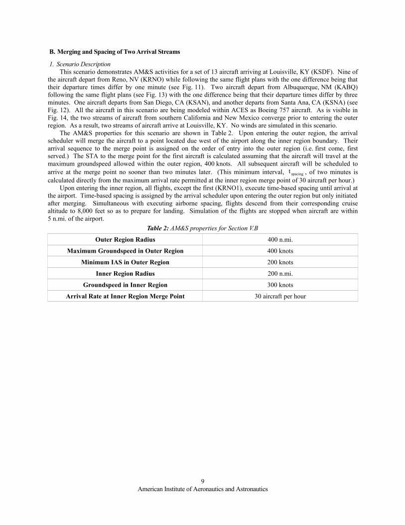
1. Scenario DescriptionThis scenario demonstrates AM&S activities for a set of 13 aircraft arriving at Louisville, KY (KSDF). Nine of

the aircraft depart from Reno, NV (KRNO) while following the same flight plans with the one difference being that their departure times differ by one minute (see Fig. 11). Two aircraft depart from Albuquerque, NM (KABQ) following the same flight plans (see Fig. 13) with the one difference being that their departure times differ by three minutes. One aircraft departs from San Diego, CA (KSAN), and another departs from Santa Ana, CA (KSNA) (see Fig. 12). All the aircraft in this scenario are being modeled within ACES as Boeing 757 aircraft. As is visible in Fig. 14, the two streams of aircraft from southern California and New Mexico converge prior to entering the outer region. As a result, two streams of aircraft arrive at Louisville, KY. No winds are simulated in this scenario.

The AM&S properties for this scenario are shown in Table 2. Upon entering the outer region, the arrival scheduler will merge the aircraft to a point located due west of the airport along the inner region boundary. Their arrival sequence to the merge point is assigned on the order of entry into the outer region (i.e. first come, first served.) The STA to the merge point for the first aircraft is calculated assuming that the aircraft will travel at the maximum groundspeed allowed within the outer region, 400 knots. All subsequent aircraft will be scheduled to arrive at the merge point no sooner than two minutes later. (This minimum interval, t spacing , of two minutes is calculated directly from the maximum arrival rate permitted at the inner region merge point of 30 aircraft per hour.)

Upon entering the inner region, all flights, except the first (KRNO1), execute time-based spacing until arrival at the airport. Time-based spacing is assigned by the arrival scheduler upon entering the outer region but only initiated after merging. Simultaneous with executing airborne spacing, flights descend from their corresponding cruise altitude to 8,000 feet so as to prepare for landing. Simulation of the flights are stopped when aircraft are within 5 n.mi. of the airport.

Table 2: AM&S properties for Section V.B

Outer Region Radius 400 n.mi.

Maximum Groundspeed in Outer Region 400 knots

Minimum IAS in Outer Region 200 knots

Inner Region Radius 200 n.mi.

Groundspeed in Inner Region 300 knots

Arrival Rate at Inner Region Merge Point 30 aircraft per hour


Louisville

Albuquerque

Reno

San Diego

Santa Ana

Figure 10. Overview of flight routes from Reno, NV, San Diego, CA, Santa Ana, CA, and Albuquerque, NM to Louisville, KY.

KRNO1KRNO2

KRNO3KRNO4

KRNO5KRNO6

KRNO7KRNO8

KRNO9

Reno

Figure 11. Aircraft locations departing from Reno, NV.

Santa Ana

San Diego

KSNA1

KSAN1

Figure 12. Aircraft locations departing from San Diego, CA and Santa Ana, CA.

Albuquerque

KABQ1KABQ2

KSNA1KSAN1

Figure 13. Aircraft locations departing from Albuquerque, NM.


KRNO1KRNO2

KRNO3KRNO4

KRNO5KRNO6

KRNO7KRNO8

KRNO9

KSNA1KSAN1 KABQ1

KABQ2

Figure 14. Aircraft routes before entering the outer region. Note that the routes for the four southern flights converge to a common route before entering the outer region.

2. Scenario ResultsTable 3 shows various times for the simulated flights. These times include the time of takeoff; the time of

entering the outer region; the STA to the inner merge point as issued by the arrival scheduler; the actual time of arrival to the inner merge point as executed by the aircraft, and whether a delaying maneuvering was inserted by the aircraft in order to achieve that arrival time. Note that some of the flights inserted a delaying maneuver upon receiving a STA from the arrival scheduler. These delaying maneuvers took the form of a holding pattern on the right-side of the original route (see Fig. 15).

Figure 15 shows the aircraft locations prior to the first flight (KRNO1) arriving at the merge point. The figure clearly shows how the stream of nine flights from Reno, NV create gaps along their route that will be filled in by the four other flights at the merge point.

Figure 16 shows the aircraft locations after all the flights have merged to a single stream within the inner region. Note how the aircraft are equally spaced. Figure 18 shows the time-based spacing of each flight relative to the first flight (KRNO1) while passing through the inner region. Note how the aircraft are spaced two-minutes apart.

Figure 17 shows the groundspeed of each aircraft upon entering the outer region. There are two speed transitions for each flight. The first speed transition occurs when the flight enters the outer region as it alters its speed such that it arrives at its STA to the merge point. The second speed transition occurs when the flight enters the inner region (after merging) and executes time-based spacing relative to the lead aircraft assigned by the arrival scheduler. Note the second speed transitions are marked by spikes in the speeds when airborne spacing is initially engaged. These speeds spikes are a result of the initial relative speeds of the lead aircraft, which is coming from one direction, relative to the trailing aircraft, which is coming from another direction. This behavior is not exhibited by the first aircraft to the merge point, KRNO1, since it has no lead aircraft to follow. Neither is it exhibited by the second aircraft to the merge point, KABQ1, because its original flight direction to the east is largely maintained as it moves in behind KRNO1. This speed spike behavior begins when the third aircraft to the merge point, KRNO2, moves behind KABQ1. This is a result of the ability of KRNO1 to maintain its easterly flight while KRNO2 must turn from the southeast to the east. During this turn, KABQ1 is relatively speeding away. Since the speed control is partly a function of the relative speed, a higher speed is commanded. The aircraft surges to the east, then overshoots its location behind KABQ1, and finally settles in behind it. This behavior repeats for all subsequent flights from the northwest (i.e. all those from KRNO). The remaining flights from the west (i.e.KABQ1, KSNA1, and KSAN1) exhibit the opposite behavior in that they initially get too close to their lead aircraft. Again, those lead aircraft,


which are coming from the northwest, are initially moving too slowly to the east because they are still turning left towards the east.

Table 3: Data for Section V.B. Flights are sorted by arrival times to the merge point.

Flight Takeoff Time Outer Region Entry Time

Scheduled Time of Arrival to Inner Region Merge Point

Delay Maneuver Inserted by

Flight

Actual Time of Arrival to Inner Region Merge

Point

KRNO1 01:21:00 EDT 03:54:00 EDT 04:28:12 EDT No 04:28:20 EDT

KABQ1 02:28:00 EDT 03:55:00 EDT 04:30:12 EDT Yes 04:30:15 EDT



KABQ2 02:31:00 EDT 03:58:00 EDT 04:36:12 EDT Yes 04:36:15 EDT




KSNA1 01:28:00 EDT 04:03:00 EDT 04:44:12 EDT Yes 04:44:10 EDT

KRNO5 01:28:49 EDT 04:04:00 EDT 04:46:12 EDT Yes 04:46:10 EDT


KSAN1 01:34:00 EDT 04:05:00 EDT 04:50:12 EDT Yes 04:50:10 EDT


KRNO1

KRNO2KRNO3

KRNO4KRNO5

KRNO6

KRNO7KRNO8

KRNO9

KABQ1KABQ2KSNA1KSAN1

Figure 15. Aircraft locations prior to the first aircraft (KRNO1) arriving at the merge point.

KRNO1

KRNO2KRNO3

KRNO4

KRNO5KRNO6

KRNO7KRNO8

KRNO9

KABQ1

KABQ2

KSNA1

KSAN1

Figure 16. Aircraft locations prior to the first aircraft (KRNO1) arriving at the merge point.


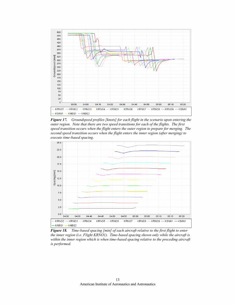
Figure 17. Groundspeed profiles [knots] for each flight in the scenario upon entering the outer region. Note that there are two speed transitions for each of the flights. The first speed transition occurs when the flight enters the outer region to prepare for merging. The second speed transition occurs when the flight enters the inner region (after merging) to execute time-based spacing.

Figure 18. Time-based spacing [min] of each aircraft relative to the first flight to enter the inner region (i.e. Flight KRNO1). Time-based spacing shown only while the aircraft is within the inner region which is when time-based spacing relative to the preceding aircraft is performed.


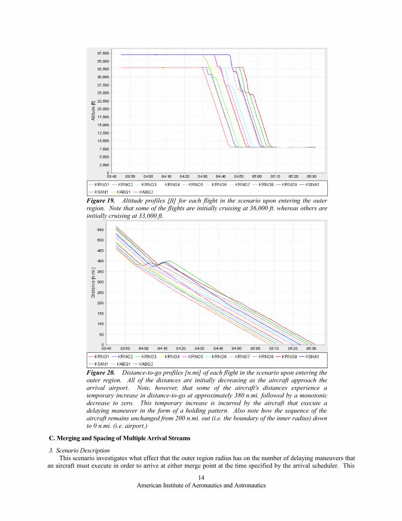
Figure 19. Altitude profiles [ft] for each flight in the scenario upon entering the outer region. Note that some of the flights are initially cruising at 36,000 ft. whereas others are initially cruising at 33,000 ft.

Figure 20. Distance-to-go profiles [n.mi] of each flight in the scenario upon entering the outer region. All of the distances are initially decreasing as the aircraft approach the arrival airport. Note, however, that some of the aircraft's distances experience a temporary increase in distance-to-go at approximately 380 n.mi. followed by a monotonic decrease to zero. This temporary increase is incurred by the aircraft that execute a delaying maneuver in the form of a holding pattern. Also note how the sequence of the aircraft remains unchanged from 200 n.mi. out (i.e. the boundary of the inner radius) down to 0 n.mi. (i.e. airport.)

C. Merging and Spacing of Multiple Arrival Streams

3. Scenario DescriptionThis scenario investigates what effect that the outer region radius has on the number of delaying maneuvers that

an aircraft must execute in order to arrive at either merge point at the time specified by the arrival scheduler. This


will be investigated by simulating a set of 61 aircraft arriving at Louisville International Airport (KSDF) and departing from airports across the U.S. The flight routes used were the actual routes and cruise altitudes flown on May 17, 2002 to Louisville, KY although shifted in time in order to increase traffic density during a few hours of the day. All the aircraft in this scenario are being modeled within ACES as Boeing 727 Stage 3 aircraft. Finally, no winds are simulated in this scenario.

The AM&S properties used for this scenario are shown in Table 2. Note that the outer region radius is being used as a parameter for each run of the simulation. The number of flights that implement a delaying maneuver is then reported for each outer region radius that is simulated.

Upon entering the outer region, the arrival scheduler instructs all aircraft to merge to either of two points along the inner region boundary: due west of the airport, or due east of the airport. Flights arriving from the east are assigned to the eastern merge point, and flights arriving from the west are assigned to the western merge point. In effect, there are two outer regions: an eastern half and a western half. Their arrival sequence to each merge point is assigned on the order of entry into either the eastern or western outer region (i.e. first-come, first-served.)

Table 4: AM&S properties for Section V.C

Outer Region Radius See Table 5

Maximum Groundspeed in Outer Region 400 knots

Minimum IAS in Outer Region 200 knots

Inner Region Radius 60 n.mi.

Groundspeed in Inner Region 300 knots

Arrival Rate at Inner Region Merge Point 30 aircraft per hour

Figure 21. Aircraft routes around Louisville International Airport with a 20 n.mi. inner region radius and a 40 n.mi. outer region radius. Note the holding patterns that must be performed by some flights in order to arrive at the eastern merge point at the time issued by the arrival scheduler.


Routes

HoldingPatterns

Louisville

EasternMerge Point

Outer RegionBoundary

Inner RegionBoundary

4. Scenario ResultsTable 5 displays the number of flights that implement a delaying maneuver as a function of the outer region

radius. As the outer region radius increases, the number of delaying maneuvers is observed to decrease. This was expected because the larger outer radius results in longer distances between all points along the outer region boundary and the merge point located on the inner region. Longer distances require linearly more time to traverse if speed remains constant. Despite the longer distances, the delaying maneuvers did not decrease to zero as the outer region radius increased to 200 n.mi.

Table 5: Number of Delaying Maneuvers as a Function of the Outer Region Radius

Outer Region Radius [n.mi.] Number of Delaying Maneuvers

80 15

100 11

120 10

140 7

160 5

180 4

200 4An explanation for the persistence of delaying maneuvers can be found by inspecting the scenario when the

outer radius was set to 80 n.mi. A summary of the data for flights assigned to the western merge point can be found in Table 7. All aircraft entered the outer region along different points of the outer region. Consequently, the distance to the merge point was different for each aircraft. The arrival scheduler scheduled times-of-arrivals such that all flights were separated in time at the merge point by at least 2 minutes. (This minimum interval of two minutes was calculated directly from the maximum arrival rate permitted at the inner region merge point of 30 aircraft per hour.) The difference between the STA and the rerouting time is the scheduled travel duration allotted to the aircraft. The quotient of the distance to the merge point with the scheduled travel duration is the average scheduled groundspeed for a direct route between the aircraft's current location to the merge point.

In order to determine whether a delaying maneuver is required, the scheduled groundspeed must be compared with the minimum permissible IAS of 200 knots. However, for proper comparison, these speeds must be expressed in a common speed frame. The common speed frame used in Table 7 is that of groundspeed. The conversion of indicated airspeed to groundspeed takes into account four factors: (a) calibration errors of the speed sensor aboard the aircraft; (b) variations of air density with temperature; (c) variations of air density with pressure; and, (d) winds. In this work, the following assumptions were made: (a) aircraft have perfectly calibrated speed sensors; (b) aircraft fly within a standard atmosphere; and (c) there are no winds. Therefore, the indicated airspeed was influenced solely by the variation of air density with respect to temperature and pressure as a function of altitude. This variation is well defined by the International Standard Atmosphere. With these assumptions, Table 6 displays the the equivalent groundspeed of 200 knots IAS at different altitudes above mean sea level.

Table 6: Groundspeed as a function of altitude for aircraft traveling at 200 knots IAS

0 [feet] 10,000 [feet] 20,000 [feet] 30,000 [feet] 40,000 [feet]

200 knots 232 knots 271 knots 319 knots 385 knotsThe data in Table 7 indicates that the aircraft requiring delaying maneuvers had scheduled groundspeeds less

than the minimum permissible groundspeed for the aircraft's cruise altitude. (This is to be expected because, as defined in Section III.D, this was the trigger for requiring a delaying maneuver.) Similarly, the aircraft that did not require delaying maneuvers had scheduled groundspeeds greater than the minimum permissible groundspeed. These observations held for all of the flights in all of the scenarios. The reader is reminded that the fastest aircraft within the outer region will have an average groundspeed of 400 knots. All other aircraft that need to delay must travel slower than this speed. In this scheme of merging and spacing, an aircraft traveling at 40,000 feet can only slow down by 15 knots (see Table 6) in order to avoid a delaying maneuver.


Table 7: Data for flights directed to the western merge point for Section V.C

Flight Outer Region Entry Time

Flight to Follow within Inner

Region

Scheduled Time of

Arrival to Inner Region Merge Point

Scheduled Travel

Duration to Merge Point

[s]

Distance to Merge Point

[n.mi.]

Scheduled Groundspeed [knots]

Cruise Altitude

[feet]

Minimum Permissible Groundspeed at Cruise

Altitude [knots](Converted from 200 knots IAS)

Delay Maneuver Inserted by Flight

35 23:35:00 23:36:33 93 10.35 400 29,000 314 No36 0:24:00 0:30:20 380 42.22 400 29,000 314 No42 0:54:00 1:00:12 372 41.34 400 23,000 284 No37 0:56:00 1:08:46 766 85.15 400 33,000 336 No50 1:31:00 1:37:21 381 42.38 400 29,000 314 No44 1:42:00 1:43:20 80 8.92 400 33,000 336 No49 2:00:00 2:14:02 842 93.61 400 14,000 246 No75 2:12:00 49 2:16:02 242 12.08 179 25,000 293 Yes47 2:16:00 75 2:18:02 122 8.77 258 33,000 336 Yes73 2:19:00 2:26:51 471 52.34 400 25,000 293 No39 2:29:00 2:30:50 110 12.28 400 37,000 361 No54 2:34:00 2:35:13 73 8.16 400 33,000 336 No87 2:49:00 2:50:55 115 12.78 400 27,000 303 No84 3:05:00 3:14:08 548 60.94 400 33,000 336 No86 3:14:00 3:22:09 489 54.38 400 37,000 361 No88 3:47:00 3:59:11 731 81.21 400 37,000 361 No89 3:50:00 88 4:01:11 671 7.44 40 33,000 336 Yes91 3:50:00 89 4:03:11 791 79.93 364 33,000 336 No76 4:19:00 4:27:08 488 54.27 400 33,000 336 No92 4:25:00 76 4:29:08 248 8.42 122 37,000 361 Yes59 4:35:00 4:42:57 477 53.03 400 33,000 336 No85 4:38:00 59 4:44:57 417 11.87 102 33,000 336 Yes52 4:41:00 4:47:20 380 42.27 400 37,000 361 No65 4:47:00 52 4:49:20 140 8.91 228 37,000 361 Yes


69 4:49:00 65 4:51:20 140 12.49 320 33,000 336 Yes66 5:00:00 5:07:54 474 52.70 400 33,000 336 No79 5:04:00 66 5:09:54 354 12.18 124 33,000 336 Yes78 5:09:00 79 5:11:54 174 8.05 166 33,000 336 Yes82 5:24:00 5:25:23 83 9.29 400 33,000 336 No83 5:24:00 5:30:19 379 42.12 400 33,000 336 No


VI. ConclusionIn this effort, we successfully developed, prototyped and demonstrated a simulation testbed for merging and

spacing in NASA’s Airspace Concept Evaluation System (ACES) software to support NASA’s Airportal research. The merging and spacing modules consists of two components: a ground-based scheduling tool that generates arrival sequences and spacing requirements for aircraft entering a terminal airspace; and, an airborne component that merges aircraft, as necessary, and then maintains the requisite spacing within the merged stream. We demonstrated the feasibility of using the simulation testbed to investigate airborne merging and spacing, and the effect of control horizons on the ability of aircraft to absorb delays.

It is interesting to consider the available options for delaying an aircraft's arrival. Two approaches evaluated in this work and demonstrated in these scenarios were to slow an aircraft at its current altitude, and to insert delaying maneuvers at an aircraft's current altitude. An alternative that might be considered in future work is for an aircraft to descend to lower altitudes where slower groundspeeds are feasible with less risk of stalling. Interestingly, this is a side effect of what occurs when ATC directs aircraft to perform stepped descents for arrival.

AcknowledgmentsWe would like to thank Yingchuan Zhang, a Research Scientist at Intelligent Automation Inc., for her assistance

and insight with investigating the root cause of the delaying maneuvers in Section V.C.

References1United States Government Accountability Office, "National Airspace System Modernization: Observations on Potential Funding Options for FAA and the Next Generation Airspace System", GAO-06-1114T, 2006.2EUROCONTROL/FAA, "Principles of Operation for the Use of Airborne Separation Assurance Systems", EUROCONTROL/FAA Cooperative R&D Edition 7.1, 2001.3Meyn, L., Windhorst, R., Roth, K., Van Drei, D., Kubat, G., Manikonda, V., Roney, S., Hunter, G., Huang, A., Couluris, G., "Build 4 of the Airspace Concept Evaluation System", AIAA Modeling and Simulation Technologies Conference and Exhibit, 21-24 August 2006.4RTCA SC-186, "Minimum Aviation System Performance Standards for Automatic Dependent Surveillance Broadcast (ADS-B)", RTCA/DO-242A, 2002.5RTCA SC-186, "Guidance for Initial Implementation of Cockpit Display of Traffic Information", RTCA/DO-243, 1998.6Garren, J.F., Moen, G.C., "Cockpit Display of Traffic Information (CDTI)", Proceedings of the American Society for Information Science Symposium, Pittsburgh, Pa., May 1980.7Hart, S.G., Wempe, T.E., "Cockpit Display of Traffic Information: Airline Pilot's Options About Content, Symbology, and Format", NASA TM 78601, Aug. 1979.8Palmer, E.A. et al., "Perception of Horizontal Aircraft Separation on a Cockpit Display of Traffic Information", Human Factors, Vol. 22, No. 5, Oct. 1980, pp. 605-620.9Abbott, T.S. et al., "Flight Investigation of Cockpit Displayed Traffic Information Utilizing Coded Symbology in an Advanced Operational Environment", NASA TP 1683, July 1980.10Sorensen, J.A., and Tsuyoshi, G., "Analysis of In-Trail Following Dynamics of CDTI-Equipped Aircraft", Journal of Guidance, , 1983, Vol.6, No.3, p.162.11Abbott, T.S., "Speed Control Law for Precision Terminal Area In-Trail Self Spacing", NASA TM 211742, 2002.12Hoffman, E., Ivanescu, D., Shaw, C., Zeghal, K., "Analysis of Constant Time Delay Airborne Spacing Between Aircraft of Mixed Types in Varying Wind Conditions", 5th USA/Europe Air Traffic Management R&D Seminar, Budapest, Hungary, 23-27 June 2003.13Ivanescu, D., Hoffman, E., Zeghal, K., "Impact of ADS-B Link Characteristics on the Performances of In-Trail Following Aircraft", AIAA Guidance, Navigation, and Control Conference and Exhibit, 5-8 August 2002.14Wang, G., Hammer, J., "Analysis of an Approach Spacing Application", MITRE Corporation, 2001.15Oseguera-Lohr, R., Lohr, G., Abbot, T., Eischeid, T., "Evaluation of Operational Procedures for Using a Time-Based Airborne Inter-Arrival Spacing Tool", AIAA's Aircraft Technology, Integration, and Operations (ATIO) 2002 Technical, 1-3 October 2002, Los Angeles, California, 2002.16Pritchett, A.R., Yankosky, L.J., "Pilot-Performed In-Trail Spacing and Merging: An Experimental Study", Journal of Guidance, Control, and Dynamics, Vol. 26, No. 1, January-February 2003, pp. 143-150.17Lohr, G., Oseguera-Lohr, R., Abbot, T., Capron, W., "Flight Evaluation of a Time-Based Airborne Inter-Arrival Spacing Tool", 5th USA/Europe Air Traffic Management R&D Seminar, Budapest. 23-27 June 2003, 2003.18Grimaud, I., Hoffman, E., Rognin, L., Zeghal, K., "Spacing Instructions in approach: Benefits and limits from an air traffic controller perspective", AIAA Guidance, Navigation, and Control Conference and Exhibit, 16-19 August 2004, Providence, Rhode Island, 2004.19Callantine, T., Lee, P., Mercer, J., Prevot, T., "Terminal-Area Traffic Management with Airborne Spacing", AIAA 5th Aviation, Technology, Integration, and Operations Conference (ATIO), 26-28 September 2005, Arlington, VA, 2005.


20Boursier, L., Hoffman, E., Rognin, L, Vergne, F., Zeghal, K., "Airborne Spacing in the Terminal Area: A Study of Non-Nominal Situations", 6th AIAA Aviation Technology, Integration and Operations Conference (ATIO), 25-27 September 2006, Wichita, Kansas, 2006.21Casaux, F., Hasquenoph, B., "Operational use of ASAS", USA/Europe ATM R&D Seminar, Saclay, France, 1997.22Simons, E., Hawkins, P.S., Zeitlin, A.D., DeSenti, C.T., "Controller Assigned Airborne Separation (CAAS) Concept Exploration", AIAA 4th Aviation Technology, Integration and Operations (ATIO) Forum, 20-22 September 2004, Chicago, IL, 2004.23Hoffman, E., Grimaud, I., Rognin, L., Zeghal, K., "Delegation of Crossing Operations to the Flight Crew: First Quantitative Results", AIAA Guidance, Navigation, and Control Conference and Exhibit, 6-9 August 2001, Montreal, Canada, 2001.24Duong, V.N., "FREER: Free-Route Experimental Encounter Resolution - A Solution for the European Free Flight Implementation?", Air Navigation Conference, Amsterdam, Netherlands, 1997.25Hoekstra, J.M., van Gent, R.N.H.W., Ruigrok, R.C.J., "Conceptual Design of Free Flight with Airborne Separation Assurance", AIAA Guidance, Navigation, and Control Conference and Exhibit, Boston, MA, 10-12 August 1998.26NASA, "Concept Definition for Distributed Air-Ground Traffic Management (DAG-TM), v.1.0", Advanced Air Transportation Technologies (AATT) Project, M/S 262-4, NASA Ames Research Center, Moffett Field, CA 94035, September 1999.27NASA, "Research Plan for Distributed Air-Ground Traffic Management (DAG-TM), v.1.01", Advanced Air Transportation Technologies (AATT) Project, M/S 262-4, NASA Ames Research Center, Moffett Field, CA 94035, September 1999.28Green, S.M., Bilimoria, K.D., Ballin, M.G., "Distributed Air-Ground Traffic Management for En Route Flight Operations", AIAA Guidance, Navigation, and Control Conference, Denver, CO, 14-17 August 2000.29Billimoria, K.D., "A Geometric Optimization Approach to Aircraft Conflict Resolution", AIAA Guidance, Navigation, and Control Conference and Exhibit, Denver, CO, 14-17 August 2000.30Wing, D.J., Barmore, B.E., "Use of Traffic Intent Information by Autonomous Aircraft in Constrained Operations", AIAA Guidance, Navigation, and Control Conference and Exhibit, 5-8 August 2002, Monterey, CA, 2002.31Mondoloni, S., Conway, S., "An Airborne Conflict Resolution Approach Using a Genetic Algorithm", AIAA Guidance, Navigation, and Control Conference and Exhibit, 6-9 August 2001, Montreal, Canada, 2001.32Vivona, R.A., Karr, D.A., Roscoe, D.A., "Pattern-Based Genetic Algorithm for Airborne Conflict Resolution", AIAA Guidance, Navigation, and Control Conference and Exhibit, 21-24 August 2006, Keystone, CO, 2006.33Ballin, M.G., Wing, D.J., Hughes, M.F., Conway, S.R., "Airborne Separation Assurance and Traffic Management: Research of Concepts and Technology", AIAA Guidance, Navigation, and Control Conference and Exhibit, Portland, OR, 9-11 August 1999.34Bilimoria, K.D., "A Geometric Optimization Approach to Aircraft Conflict Resolution", AIAA Guidance, Navigation, and Control Conference and Exhibit, Denver, CO, 14-17 August 2000.35Anderson. J., Introduction to Flight (3rd ed.), McGraw Hill, Inc., pp.74-79, 117-118, 1989.


A Simulation Testbed for Airborne Merging and Spacing · spacing = duration of time-based spacing...

Documents

Transcript of A Simulation Testbed for Airborne Merging and Spacing · spacing = duration of time-based spacing...