A Simulation Study of ManagerialCompensation

Brian SallansAlexander Pfister

Georg Dorffner

Working Paper No. 101

SFB‘Adaptive Information Systems and Modelling in Economics and Management

Science’

Vienna University of Economicsand Business Administration

Augasse 2–6, 1090 Wien, Austria

in cooperation withUniversity of Vienna

Vienna University of Technology

http://www.wu-wien.ac.at/am

This piece of research was supported by the Austrian Science Foundation (FWF)under grant SFB#010 (‘Adaptive Information Systems and Modelling in Economics

and Management Science’).

Abstract

A computational economics model of managerial compensation is presented.Risk-averse managers are simulated, and shown to adopt more risk-taking un-der the influence of stock options. It is also shown that stock options can bothhelp a new entrant compete in an established market; and can help the incum-bent firm fight off competition by promoting new exploration and risk-taking.In the case of the incumbent, the stock options are shown to be most effectivewhen introduced as a response to the arrival of a new entrant, rather than usedas a standard part of the compensation package.

1 Introduction

Designing compensation for top-level managers is an important aspect of firm governance. Under-standing compensation contracts is therefore of great general interest. Specifically, we focus on therole of stock options as part of a compensation contract.

Theoretical models of compensation address the problem of how to craft contracts which maxi-mize firm value. Principal-Agency models have achieved some prominence as a model of contracts,including those between managers and owners of a company [Holmstrom 1979]. The key feature ofprincipal-agency models is that the principal is limited in terms of the observability of the agent’sactions, effort, results, or preferences. The principal therefore delegates decision making to the agent.Alternatively, compensation models can focus on how contracts or instruments are valued by man-agers as opposed to unrestricted traders (see for example Hall and Murphy [2002]).

Typically, the manager in a theoretical model of compensation is assumed to be a fully rationaleconomic actor. She has complete knowledge and understands the consequences of her actions, atleast probabilistically. She can therefore assess the riskiness of alternative actions, and weigh thisagainst possible gains in her compensation. This assumption results in analytic models for which thecontract can be found which optimizes the gain by the firm’s owners [Bushman and Indjejikian 1993;Baiman and Verrecchia 1995; Choe 1998].

One limitation of principal-agency models is there restriction to rational agents. Empirical workseeks to address this limitation by studying the influence of compensation in actual firms. However,real firms are complicated. It is difficult to control for all variables in an empirical study. Empiricalstudies of compensation have led to conflicting and inconclusive results [Murphy 1999].

Beginning with the work of Herbert Simon [1982], there has been a realization that classicaleconomic theory, based on full rationality, is limited. In reality, economic agents are bounded both intheir knowledge and in their computational abilities. Recent work in simulation-based computationaleconomics has sought to implement boundedly rational economic actors as learning agents, and tostudy the implications on the resultant economic systems. See Tesfatsion [2002] for a review ofagent-based computational economics.

Computational economic models bridge the gap between theoretical and empirical economics. Onone hand, a computational model can be used to test the predictions of theory under conditions whichare too complex to be addressed analytically. On the other hand, computational models can be usedto give insight into complex systems and suggest new hypotheses to be tested in empirical studies.Computational models offer an environment which is complex but controlled, where all assumptions

1

are explicitly encoded in the model.In this article we study management compensation using a discrete-time agent-based economic

model. The model spans two markets: a consumer market and a financial equities market. The con-sumer market consists of production firms offering a good for sale, and customers who can purchasethe good. The financial equities market consists of stock traders who can buy and sell shares in theproduction firms. This model is called the integrated markets model (IMM).

The IMM is intended to be a generic model of the interaction between financial and consumer mar-kets. It has been shown to reproduce a large range of empirical “stylized facts”, including learning-by-doing in the consumer market; low predictability, high kurtosis and volatility clustering in the financialmarket; and correlations between volatility and trading volume in the financial market. See Sallans,Pfister, Karatzoglou, and Dorffner [2003] for a detailed description of the model and experimentalsimulation and validation results. It has been used previously to simulate the influence of financialtraders’ expectations on the behavior of managers [Sallans, Dorffner, and Karatzoglou 2002].

The managers of the firms in the IMM try to optimize their own compensation. Depending ontheir contract, they might do this by increasing profits, or by taking actions which they predict willmore directly boost the value of their stock-based compensation. Thus, as in principal-agency models,the problem of moral hazard still exists in the IMM. However, each manager explicitly implementsa boundedly-rational agent which learns from experience, and itself has limited knowledge and com-putational power. We supplement the classical principal-agency framework by considering issues oflimited knowledge, learning from experience, exploration versus exploitation of existing knowledge,and asymmetry between different sources of information for the decision-making agent. We use arti-ficial intelligence techniques to implement learning and decision-making in the firm.

Under the IMM, the role of the compensation contract is somewhat different than under a principal-agency framework. The manager does not start with intimate knowledge of the consumer or financialmarket. Rather, it must learn what the markets want through experience. The manager receives feed-back in terms of profits and movements in stock price. These two measures give the manager twodifferent views of firm performance. Because these two estimators are generated by two differentpopulations of boundedly-rational agents (consumers and stock traders respectively), they do not nec-essarily agree.

The appeal of using the IMM to investigate compensation is that it was not explicitly built forthis purpose. It is a system consisting of firms, consumers and stock traders. In the IMM there is noexplicit link between, for example, stock option value and risk-taking. A manager takes actions in theconsumer market. Stock traders observe the results of these actions, and buy or sell stock. A priori,it is not clear to what degree a manager can influence the volatility of their firm’s stock. If grantingstock options influences risk-taking in our model, and if taking risks results in improved performance,it will indicate that this is a very robust effect that occurs naturally in this type of system. This will befurther evidence for the mechanisms predicted by principal-agency theory.

In this paper we use the IMM first to test predictions of theoretical models of contracts, and secondto generate new hypotheses that can be tested empirically. Specifically, we test the effect of stockoptions on manager learning and behavior. In the first set of experiments, we test some predictionsof principle-agency theory. The goal is to see how robust these predictions are to the situation ofincomplete knowledge and learning, and to confirm that the model of learning and decision makingin the firm acts in a reasonable way. In the second set of experiments, we investigate the effect ofoption-granting on learning and new knowledge acquisition.

For completeness, we give a description of the basic model in the next sections. This is followed bya description of the different compensation schemes examined, and simulation results. We concludewith a discussion of the simulation results and their implications on managerial compensation.

2

2 The Integrated Markets Model

In this section we give a description of the integrated markets model. The reader is directed to Sallans,Pfister, Karatzoglou, and Dorffner [2003] for a detailed description of the model and validation results.

The model consists of two markets: a consumer market and a financial equities market. Theconsumer market simulates the manufacture of a product by production firms, and the purchase ofthe product by consumers. The financial market simulates trading of shares. The shares are tradedby financial traders. The two markets are coupled: The financial traders buy and sell shares in theproduction firms, and the managers of firms may be concerned with their share price. The traders canuse the performance of a firm in the consumer market in order to make trading decisions. Similarly,the production firms can potentially use positioning in product space and pricing to influence thedecisions of financial traders (see figure 1).

Consumer Financial

Market

stock tradersconsumers

Market Stock priceBuyingpatterns (stock options)

Product position Production

Firm

(fundamental price)Profits

Price

Figure 1: The Integrated Markets Model. Consumers purchase products, and financial traders tradeshares. Production firms link the consumer and financial markets, by selling products to consumersand offering their shares in the financial market.

The simulator runs in discrete time steps. Simulation steps consist of the following operations:

1. Consumers make purchase decisions.

2. Firms receive an income based on their sales and their position in product space.

3. Financial traders make buy/hold/sell decisions. Share prices are set and the market is cleared.

4. Every Np steps, production firms update their products or pricing policies based on performancein previous iterations.

We describe the details of the markets, and how they interact, in the following sections.

3 The Consumer Market

The consumer market consists of firms which manufacture products, and consumers who purchasethem. The model is meant to simulate production and purchase of non-durable goods, which the con-sumers will re-purchase at regular intervals. The product space is represented as a two-dimensional

3

simplex, with product features represented as real numbers in the range [0,1]. Each firm manufac-tures a single product, represented by a point in this two-dimensional space. Consumers have fixedpreferences about what kind of product they would like to purchase. Consumer preferences are alsorepresented in the two-dimensional product feature space. There is no distinction between productfeatures and consumer perceptions of those features.

3.1 Firms

Every Np iterations of the simulation the firms must examine market conditions and their own per-formance in the previous iterations, and then modify their product or pricing. A boundedly rationalagent can be subject to several kinds of limitations. We focus here on limits on knowledge, andrepresentational and computational power. How these limitations are implemented is detailed below.

The production firms are adaptive learning agents. They adapt to consumer preferences and chang-ing market conditions via a reinforcement learning algorithm [Sutton and Barto 1998]. Reinforcementlearning has been used to simulate firm behavior in competitive markets [Tesauro 1999], as well asto estimate optimal controllers in many contexts [Bertsekas and Tsitsiklis 1996]. It can be seen asapproximating solving for a Nash equilibrium. It is essentially a sampling-based algorithm to solve adynamic programming problem. It is used here as an alternative to a genetic algorithm as a model forlearning in the firm. Reinforcement learning is more appropriate as a model of learning within a trialand within a single firm. This is in contrast to genetic programming, which models learning within apopulation across many trials. For completeness, we detail the reinforcement learning representationand algorithm below.

3.1.1 State Description

The firms do not have complete information about the environment in which they operate. In particu-lar, they do not have direct access to consumer preferences. They must infer what the consumers wantby observing what they purchase. Purchase information is summarized by performing “k-means”clustering on consumer purchases. The number of cluster centers is fixed at the start of the simula-tion. The current information about the environment consists of the positions of the cluster centers infeature space, along with some additional information. The information is encoded in a bit-vector of“features”. The features are summarized in Table 1.

The cluster centers are encoded as binary vectors. Each cluster center can be described as a pairof numbers in [0, 1]× [0, 1]. Two corresponding binary vectors are generated by “binning”. Each axisis divided in to K bins. For all of our experiments, K was set to 10. The bit representing the binoccupied by each number is set to 1. All other bits are 0. For example, given 10 bins per axis and acluster center (0.42, 0.61), the resulting bit vector is (0 0 0 0 1 0 0 0 0 0 0 0 0 0 0 0 1 0 0 0).

This information gives a summary of the environment at the current time step. Firms make deci-sions based on the current “state”, which is a finite history of Hs bit vectors. In other words, firmsmake decisions based on a limited memory of length Hs. This limited history window represents anadditional explicit limit on the firm’s knowledge.

3.1.2 Actions

In each iteration the firms can take one of several actions. The actions are summarized in Table 2.The “Do Nothing” and “Increase/Decrease price” actions are self-explanatory. The “random” actionis designed to allow the firm to explicitly try “risky” behavior. The “Move product” actions move the

4

Table 1: Features Available to Production Firms.

Feature Description

Assets 1 if assets increased in theprevious iteration, 0 otherwise

Share Price 1 if share price increased in theprevious iteration, 0 otherwise

Mean Price 1 if product price is greater than mean priceof competitors products, 0 otherwise

Cluster Center 1 A bit-vector that encodes the positionof cluster center 1

... ...Cluster Center N A bit-vector that encodes the position

of cluster center N

features of the product produced by the firm a small distance in a direction along the chosen axis ortowards or away from the chosen cluster center. For example, if the action selected by firm i is “MoveTowards Center j” then the product is modified as follows:

bi,k,t+1 ← bi,k,t + ν (cj,k − bi,k,t) (1)

where k ∈ {1, 2} enumerates product features, and bi,k and cj,k are the kth product feature and featureof cluster center j respectively. The update rate ν ∈ (0, 1] is a small fixed constant.

3.1.3 Reward Function

A firm’s manager seeks to modify its behavior so as to maximize an external reward signal. Thereward signal takes the form of a fixed reward, a variable amount based on the firm’s profitability, anda variable amount due to change in the value of the firms stock. The reward received by firm i at timet is given by:

ri,t = Sf + αφΦi,t + αg (pi,t − pi,t−1) (2)

where Sf is the fixed reward, Φi,t denotes the profits of firm i at time t, and pi,t denotes the shareprice of firm i at time t. In our model we assume no costs, so profits are simply the number of itemssold times the price per item. Assets are the accumulation of profits. For all of our experiments, Sf

was set to zero for simplicity. The constants αφ and αg sum to unity. They are fixed at the beginningof the simulation and held constant throughout. They trade off the relative importance of profits andstock price in a firm’s decision-making process. The constant reward signal Sf can be interpretedas a fixed salary paid to the manager of the firm. The profit-based reward can be interpreted as anperformance-based bonus given to the manager of the firm, and the stock-based reward as a stockgrant or stock option.1

1The stock based reward changes linearly with stock return. This would be consistent with a limited stock grant, or witha call option where the current price of the underlying stock is significantly above the strike price of the option.

5

Table 2: Actions Available to Production Firms.

Action Description

Random Action Take a random action from oneof the actions below, drawn froma uniform distribution.

Do Nothing Take no actions in this iteration.Increase Price Increase the product price by 1.Decrease Price Decrease the product price by 1.Move down Move product in negative Y direction.Move up Move product in positive Y direction.Move left Move product in negative X direction.Move right Move product in positive X direction.Move Towards Center 1 Move the product features

towards cluster center 1.... ...Move Towards Center N Move the product features

towards cluster center N.

3.1.4 Utility Function

Given the state history of the simulator for the previous Hs time steps, a production firm makesstrategic decisions based on its utility function. Utility functions (analogous to “cost-to-go” functionsin the control theory literature, and value functions in reinforcement learning) are a basic component ofeconomics, reinforcement learning and optimal control theory [Bertsekas and Tsitsiklis 1996; Suttonand Barto 1998]. Given the “reward signal” or payoff rt at each time step, the learning agent attemptsto act so as to maximize the total expected discounted reward, called expected discounted return,received over the course of the task:2

Rt = E

[∞∑

τ=t

γτ−trτ

]

π

(3)

Here E [·]π denotes taking expectations with respect to the distribution π, and π is the policy of thefirm. The policy is a mapping π : S → ∆|A| from states to distributions over actions. In our case Sis the set of possible state histories, and A is the set of possible actions taken by a firm. The range ofthe policy ∆|A| is the set of probability distributions over actions in A. Note that the discount factorγ encodes how “impatient” the firm is to receive reward. It dictates how much future rewards aredevalued by the agent. If desired, the discount factor can be set to the rate of inflation or the interestrate in economic simulations, such that the loss of interest on deferred earnings is taken into accountby the firm’s manager. In our simulations, the discount factor was found using the Markov chainMonte Carlo validation technique (see Sallans, Pfister, Karatzoglou, and Dorffner [2003]).

Given the above definitions, the action-value function (or Q-function [Watkins 1989; Watkins and

2We will drop the firm index i in this section for clarity. The same reinforcement learning algorithm is used for eachfirm, with the same parameter settings. Each firm learns its own value function from experience.

6

Dayan 1992]) is defined as the expected discounted return conditioned on the current state and action:

Qπ(s, a) = E

[∞∑

τ=t

γτ−trτ |st = s, at = a

]

π

(4)

where st and at denote the current state information and action respectively (see tables 1 and 2). Theaction-value function tells the firm how much total discounted reward it should expect to receive,starting now, if it executes action a in the current state s, and then follows policy π. In other words, itis the firm’s expected discounted utility (under policy π) conditioned on the current state and the nextaction. Note that this is not a myopic measure of reward. This utility function takes into account allfuture (discounted) rewards.

The coding scheme used for world states makes the overall state space quite large. However, inpractice, the number of world states observed during a typical simulation is not very large. We cantherefore represent the action-value function as a table indexed by unique state histories of length Hs

and actions.

3.1.5 Reinforcement Learning

Reinforcement learning provides a way to estimate the action-value function from experience. Basedon observations of states, actions and rewards, the learner can build up an estimate of the long termconsequences of its actions.

By definition, the action-value function at time t− 1 can be related to the action-value function attime t:

Qπ(s, a) = E

[∞∑

τ=t−1

γτ−t+1rτ |st−1 = s, at−1 = a

]

π

(5)

= E [rt−1|st−1 = s, at−1 = a]π + γE

[∞∑

τ=t

γτ−trτ |st−1 = s, at−1 = a

]

π

(6)

= E [rt−1|st−1 = s, at−1 = a]π

+γ∑

s′,a′

P (st = s′|st−1 = s, at−1 = a)π(at = a′|st = s

′)Qπ(s′, a′) (7)

The first line is just the definition of the action-value function. The second line simply unrolls theinfinite series one step, and the third line explicitly replaces the second term by the expected action-value function, again by the definition of expectations under policy π. The last line is called theBellman equations [Bellman 1957]. It is a set of self-consistency equations (one for each state-actionpair) relating the utility at time t to the utility at time t− 1.

One way to compute the action-value function is to solve the Bellman equations. We use a rein-forcement learning technique called SARSA [Rummery and Niranjan 1994; Sutton 1996]. SARSAcan be viewed as using a Monte Carlo estimate of the expectations in Eq.(7) in order to iterativelysolve the Bellman equations. At time t, the estimate of the action-value function Qt(s, a) is updatedby:

Qπt (st−1, at−1) = (1− λ)Qπ

t−1(st−1, at−1) + λ(rt−1 + γQπ

t−1(st, at))

(8)

where λ is a small learning rate. For all of our experiments, λ was set to 0.1. In words, the utilityfunction is updated as a linear mixture of two parts. The first part is the previous estimate. The second

7

part is a Monte Carlo estimate of future discounted return. It includes a sample of the reward at timet − 1 (instead of the expected value of the reward), and the utility for a sampled state and action attime t (instead of the expected utility based on the policy and state transition probability). Finally, thecurrent estimate of the action-value function is used, in place of the true action-value function.

Intuitively this learning rule minimizes the squared error between the action-value function anda bootstrap estimate based on the current reward and the future discounted return, as estimated bythe action-value function. Theoretically, this technique has been closely linked to stochastic dynamicprogramming and Monte Carlo approximation techniques [Bertsekas and Tsitsiklis 1996; Sutton andBarto 1998].

After each action-value function update, a new policy π′ is constructed from the updated action-value function estimate:

π′(a|s)← exp (Qπ(s, a))∑

a′ exp (Qπ(a′|s))(9)

This policy selects actions under a Boltzmann distribution, with better actions selected more fre-quently.

In theory, using the SARSA algorithm, the action-value function estimate will converge to theoptimal action-value function. However, convergence relies on the learner operating in a stationarystochastic Markov environment [Sutton and Barto 1998]. When there is more than one adaptive firmin the environment, the stationarity assumption is violated. Nevertheless, it has been shown that re-inforcement learning can be used to approximately solve arbitrary-sum competitive games [Tesauro1999]. As noted previously, the Markov assumption is also violated, since the state vector of the firmdoes not include all information necessary for solving the task. For example, explicit consumer pref-erences and exact product positions are not known by the firm. Such limited-memory reinforcementlearning algorithms have been used previously to approximately solve partially observable problems[Jaakkola, Singh, and Jordan 1995]. This approximation can be seen as another source of “bounded-ness” in a boundedly rational firm. As well as having a limited knowledge base (represented by thepartial state history and state aggregation), the firm has a limited model of the capabilities of otherfirms (they are assumed to have a stationary policy). Thus our firms implement an algorithm designedto iteratively improve their strategies, given the constraints on their knowledge and computationalpower.

3.2 Consumers

Consumers are defined by their product preference. Each consumer agent is initialized with a randompreference in product feature space. During each iteration of the simulation, a consumer must make aproduct purchase decision. For each available product, the consumer computes a measure of “dissat-isfaction” with the product. Dissatisfaction is a function of product price and the distance between theproduct and the consumer’s preferred product. Consumer i’s dissatisfaction with product j is givenby:

DISi,j = αc

D(βi, bj)

maxb′ D(βi, b′)+ (1− αc)

ρj

maxj ρj

(10)

where ρj denotes the price of product j, and αc trades off the importance of product features and price.For all of our experiments, alphac was set to 0.5. The measure D(βi, bj) is the Euclidean distance infeature space between the ideal product of customer i and product j:

D(βi, bj) =(βi − bj)

>W(βi − bj)

βi>Wbj

(11)

8

Here bold-faced letters denote the feature-vector representations of products and preferences. Thediagonal matrix W is common to all consumers and models the relative importance of features in thefeature space. In all of our simulations, the matrix W was initialized to the identity matrix.

Every consumer is also initialized with a “ceiling” dissatisfaction MAXDISi. The ceiling dissat-isfaction acts as a limit. If all product dissatisfactions are above its ceiling, a consumer will simplymake no purchase in that iteration. For all of our simulations, MAXDIS was set to 0.96.

Given dissatisfaction ratings for all products with dissatisfactions below the ceiling in iteration t,consumer i selects from this set the product j with the lowest dissatisfaction rating:

j = arg mink

{DISi,k} , k ∈ {l : DISi,l < MAXDISi} (12)

In order to avoid sharp boundary effects when the dissatisfaction is exceeded, the probability ofbuying the product specified in equation (12) decreases linearly from 1 to 0 as DIS goes from 0.8to 0.96. The result is that the probability of purchasing is non-zero for any dissatisfaction belowMAXDIS, and drops to zero when dissatisfaction exceeds MAXDIS.

4 The Financial Market

Our financial model is based on a standard capital market model (see e.g. [Arthur, Holland, LeBaron,Palmer, and Tayler 1997; Brock and Hommes 1998; Dangl, Dockner, Gaunersdorfer, Pfister, Soegner,and Strobl 2001; Sallans, Pfister, Karatzoglou, and Dorffner 2003; Pfister 2003]). Myopic investorsmaximize their next period’s utility subject to a budget restriction. At time t agents invest their wealthin a risky asset with price pt and in bonds, which are assumed to be risk free. Each agent only tradeswith stocks of a single firm. Within this section we therefore drop the index i for the firms. Thereare S stocks paying a dividend dt. It is assumed that firms pay out all of their profits if positive,therefore each stock gets a proportion of 1

Sof the profits. In our model dividends should be viewed as

an information signal about the fundamental situation of the firm.The risk free asset is perfectly elastically supplied and earns the risk free and constant interest rate

κ. Investors are allowed to change their portfolio in every period. The wealth of investor m at timet + 1 is given by

Wm,t+1 = (1 + κ)Wm,t + (pt+1 + dt+1 − (1 + κ) pt) qm,t (13)

where Wm,t+1 is the wealth at time t and qm,t the number of stocks of the risky asset hold at timet. As in [Brock and Hommes 1998] , [Levy and Levy 1996] , [Chiarella and He 2001] , and [Chiarellaand He 2002] the demand functions of the following models are derived from a Walrasian scenario.This means that each agent is viewed as a price taker (see [Brock and Hommes 1997] and [Grossman1989] )

Let an investor m with wealth Wm maximize his/her utility of the form

u (Wm) = −e−ζmWm (14)

with ζm as constant absolute risk aversion. Denote by Ft = {pt−1, pt−2, ..., dt−1, dt−2} the informa-tion set available at time t3. Let Em,t and Vm,t be the conditional expectation and conditional varianceof investor m at time t based on Ft. Then the demand for the risky asset qm,t solves

3Note that at time t price pt and dividend dt are not included in the information set Ft

9

Denotept: Price (ex dividend) per share of the risky asset at time tdt: Dividend at time tκ: Risk free rateS: Total number of shares of the risky assetM : Total Number of investorsqm,t: Number of shares investor m wants to hold at time tWm,t: Wealth of investor m at time tζm Risk aversion of investor m

maxqm,t

{Em,t (Wm,t+1)−

ζm

2Vm,t (Wm,t+1)

}(15)

i.e.,

qm,t =Em,t (pt+1 + dt+1)− pt (1 + κ)

ζmVm,t (pt+1 + dt+1)(16)

Let S be the total number of shares, then the market clearing price pt is implicitly given by theequilibrium equation

S =M∑

i=1

qm,t (17)

4.1 Formation of expectations

It is well known that expectations play a key role in modeling dynamic phenomena in economics.Heterogeneous expectations are introduced in the following way:

Em,t (pt+1 + dt+1) = Fm (pt−1, · · · pt−hm, dt−1, · · · , dt−hm

)

Vm,t (pt+1 + dt+1) = Gm (pt−1, · · · pt−hm, dt−1, · · · , dt−hm

)(18)

Heterogeneity arises from different information sets and different prediction functions. Agents havethree characteristics:

• Type of prediction function: Fundamentalist or chartist

• Time horizon: Length of history of past prices and dividends used for prediction

• Trade interval: Intraday trader or end-of-day trader

These characteristics are initialized at the beginning of the simulation and are held fixed thereafter.In order to keep the simulation simple, there are only two types of prediction functions and the tradeinterval can only take one out of two different values. The above three characteristics can be combinedin any way, e.g. chartists trading intraday or fundamentalists, who are end-of-day traders.

First let’s have a closer look at the type of prediction function. As in many other heterogeneousagents models we assume that two kinds of investors exist: Fundamentalists and chartists. Chartistsuse past prices to predict the future price whereas fundamentalists calculate a ”fair value” based on

10

past dividends. Therefore for a fundamentalist Ei,t (pt+1) is a function of past dividends and for achartist Ei,t (pt+1) is a function of past prices.

The second characteristic of agents is their time horizon. The time horizon is the length of historyhi of past prices and dividends used for their predictions. Time horizon means how far back agentslook into past to predict next period’s price and dividend. A long time horizon, i.e. high hi means thatmany past observations are used as a forecast. The time horizon is drawn from an uniform distribution.The range of this uniform distribution depends on the agents type of prediction function. It was foundthat for fundamentalists and chartists different time horizons were appropriate. In particular chartistshave to identify trends. The more observations they use, the further they look into the past which alsomeans that longer trends can be identified. For example, if prices followed an upward trend, thereaftera downward trend, a short term chartist, i.e. a chartist with a short time horizon, would extrapolate thedownward trend. This trader would predict a further drop in the stock price. For a long term chartistthe last two trends might cancel each other and this agent would predict no change in the stock price.However the situation for fundamentalists may be different. Fundamentalists use past dividends fortheir price prediction. Depending on the type of the dividend process, it might be favorable to basethe prediction only on the last observation. The minimum time horizon for a fundamentalist is 1, fora chartist it is 2 (the chartist needs at least 2 prices to calculate a trend, see also equation (26)). Weallow two different maximum values for the time horizon for fundamentalists and chartists. For moredetails please see the results (section 4).

The third characteristic of an agent is the trade interval φi. Investors update their portfolio everyφ periods. This corresponds to the parameter Np for the firms, which update their action every Np

periods. In our model we assume five price fixings per day with the last price setting being the closingprice of the day. Therefore every 5th, 10th, 15th etc. price is a closing price. We distinguish betweentwo types of agents concerning their trading interval: Intraday traders with φi = 1 and end-of-daytraders with φi = 5. Intraday traders update their position at every time step, whereas end-of-daytraders only trade at the closing price of each day. This means that in the first four price settingsper day only intraday traders re-balance their portfolios. In the fifth price fixing (the closing price)all agents trade. End-of-day traders ignore intraday prices, i.e. prices between their updates. Thedividends of the five previous periods are accumulated. In order to keep consistent notation betweenintraday and end-of-day traders, we will define prices and dividends as used by the intraday tradersas they are related to the highest frequency information available. Given the high-frequency price anddividend information pt and dt, the price pt−1 and dividend dt used by a trader with interval φi isgiven by:

pt−1 = pt−φi

dt =

φi−1∑

j=0

dt−j (19)

Therefore the information set used by trader i with interval φi is given by

Fhi,φi,t :

pt−φi

, pt−2φi, ..., pt−hiφi

,

φi−1∑

j=0

dt−j ,

φi−1∑

j=0

dt−φi−j , ...,

φi−1∑

j=0

dt−hiφi−j

→ {pt−1, pt−2, ..., pt−hi, dt, dt−1, ..., dt−hi

}

(20)

Now let’s have a closer look at the formation of expectation. Let’s begin with the expectation for thevariance Vi,t. Agents determine Vi,t in the following way

11

Vi,t (pt+1 + dt+1) =1

hi

hi∑

j=1

(pt−j + dt−j −M)2

with M =1

hi

hi∑

k=1

(pt−k + dt−k)

(21)

Fundamentalists and chartists have the same prediction function for the variance. Their informationset depend on their history hi of past prices and dividends and their trade interval φi.Now we take a look at the expectation of next period’s price and dividend. First we split Ei,t (pt+1 + dt+1)into Ei,t (pt+1) and Ei,t (dt+1). Investors form their expectations over the next periods dividend dt+1

in the following way:

Ei,t (dt+1) =1

hi + 1

hi∑

j=0

dt−j (22)

Fundamentalists determine their price expectation according to a model based on fundamental infor-mation, which in our model are past dividends. A fundamentalist i assumes that the fair price p

Fair pricei,t

is a linear function of past dividends, i.e.

pFair pricei,t = Fi (dt, · · · , dt−hi

)

= f1

hi + 1

hi∑

j=0

dt−j + g(23)

This leads to the following price and dividend expectation for the fundamentalist

Ei,t (pt+1 + dt+1) = (f + 1)1

hi + 1

hi∑

j=0

dt−j + g (24)

Chartists use the past history of the stock prices in order to form their expectations. They assume thatthe future price change per period equals the average price change during the last hi periods4.

Ei,t (pt+1) = pt−1 +pt−1 − pt−hi

hi − 1(25)

Note that at time t, pt is not included in the information set Ft. This leads to the following price anddividend expectation of the chartists

Ei,t (pt+1 + dt+1) = pt−1 +pt−1 − pt−hi

hi − 1+ f

1

hi + 1

hi∑

j=0

dt−j + g (26)

4.2 Sequence of Events

Let us have a look at the timing of the events within the equity market model. First the dividend dt

of the current period is announced and paid. The next step is the formation of expectations. Based onpast prices and dividends, including dt an investor i forms his/her expectation about the distribution ofthe next period’s price and dividend. According to equation (21), (24) and (26) the investor calculates

4Note that for chartists hi >= 2 for computing an average price change

12

Vm,t (pt+1 + dt+1) and Ei,t (pt+1 + dt+1). Plugging the expectations into Equation (16) the agent isable to determine the demand function, which is submitted to the stock market via limit buy ordersand limit sell orders5. After the orders of all agents are collected, the stock market calculates thisperiod’s equilibrium price pt.

The market uses a sealed-bid auction, where the clearance mechanism chooses the price at whichtrading volume is maximized. The constructed supply and demand curves are based on the transactionrequests.

The artificial return series generated by these traders exhibits the most important stylized factsfrom real markets, such as insignificant autocorrelation of returns, volatility clustering and high kur-tosis. The statistics presented in figure 2 and table 3 were computed by averaging the performance fortwo risk-neutral firms over 20 simulation runs. Figure 2 presents the mean autocorrelation coefficientsof returns and absolute returns and the errorbars correspond to the standard error of the coefficientsacross the 20 simulation runs. The autocorrelation coefficients of the returns are insignificant (exceptlag 4), and the significants of the autocorrelations of the absolute returns indicates volatility clustering.

1 2 3 4 5 6

−0.2

−0.1

0

0.1

0.2

0.3

0.4

0.5

lag

auto

corr

elat

ion

b)absolute returns

1 2 3 4 5 6

−0.2

−0.1

0

0.1

0.2

0.3

0.4

0.5

lag

auto

corr

elat

ion

a)returns

Figure 2: Autocorrelations for (a) the stock returns and (b) the absolute stock returns. The correlationsof the returns are not significant (except for lag four), and for the absolute returns are significantlypositive.

5 Compensation

Owners of a company delegate authority to a manager. The goal of the owners is to encourage themanager to increase the value of their company. The goal of the manager is to maximize its compen-sation.

In the IMM, each manager seeks to modify its behavior so as to maximize an external paymentsignal. This payment takes the form of a fixed cash salary, a variable amount based on the firm’s

5A limit order is an instruction stating the maximum price the buyer is willing to pay when buying shares (a limit buyorder), or the minimum the seller will accept when selling (a limit sell order).

13

Table 3: Summary Statistics for the Artificial Stock Returns.

Statistic Value

mean 2.9× 10−4

standard dev 2.3× 10−3

kurtosis 39.2

profitability, and a variable amount due to change in the value of the firm’s stock. We modify Eq.(2)to add compensation from stock options. The reward received by manager i at time t is given by:

ri,t = Sf + αφΦi,t + αggi + αooi (27)

where Sf is the fixed salary, Φi,t denotes the profit-based bonus at time t, and gi and oi are bonusesfrom stock grants and stock-options respectively.

For all of our experiments, Sf was set to zero for simplicity.6 The constants αφ, αg and αo arefixed at the beginning of the simulation and held constant throughout. They trade off the relativeimportance of profits and stock-based pay in a manager’s decision-making process.

5.1 Cash and Stock

A manager in the IMM is rewarded once in every time period, using a combination of cash and stock-based bonuses. Specifically, the manager’s compensation is based on a profit-based cash bonus, astock grant, and a stock option.

The profit-based bonus is proportional to the profits of the firm:

Φi,t = ci,t − ci,t−1 (28)

where ci,t are the current assets of firm i at time t.7

The stock grant bonus is proportional to the change in stock price:

gi,t = pi,t − pi,t−1 (29)

where pi,t is the stock price of firm i at time t.The value of the stock option bonus is the change in value of the stock option held by the manager:

oi,t = bi,t − bi,t−1 (30)

where bi,t is the value of the stock option held by manager i at time t. The value of the stock option iscomputed using the Black-Scholes formula. It is dependent on the current stock price; the strike price;the risk-free interest rate; the volatility of the underlying stock; and the time periods until the option

6The absolute level of salary can influence the result. For example, if the salary is much higher than the bonus, then themanager is not motivated to do anything to achieve the extra bonus. By setting the basic salary to zero, we focus on theinfluence of the bonus on manager behavior

7This is slightly unrealistic, in that all of the bonuses can be either positive or negative. In psychology, it is well knownthat positive and negative rewards do not have symmetric impacts. However, in our reinforcement learning model of firmbehavior, the sign of the reward is not significant. By centering bonuses around zero, we improve the numerical stability ofthe algorithm.

14

vests. In the following, X is the strike price; κ is the risk free interest rate; T is the number of timeperiods until the option vests; v is the per-time-period variance of the stock price; and p is the currentstock price. The function N(x) returns the cumulative probability of x being drawn from a Normaldistribution with zero mean and unit variance (it is the Normal cumulative distribution function).

C = p exp (−κ ∗ T ) (31)

s =√

v ∗ T (32)

x1 = log (p/C)/s + s/2 (33)

x2 = log (p/C)/s− s/2 (34)

b = SN(x1)− CN(x2) (35)

Black-Scholes is used because it is a commonly-used technique for option valuation of managementoptions.

5.2 Risk Aversion

In order to assess the worth and riskiness of an action, managers in the IMM estimate two quantities.First, as discussed in the model description, they estimate the expected discounted payment they willreceive after taking an action given the current world state:

Qπ(s, a) = E

[∞∑

τ=t

γτ−trτ |st = s, at = a

]

π

(36)

We have dropped the firm index i for simplicity. All firms use the same algorithms.Second, they estimate the variance of this discounted payment:

V π(s, a) = V

[∞∑

τ=t

γτ−trτ |st = s, at = a

]

π

(37)

Variance is estimated in the same way as the expected return, using stochastic dynamic programming.Given this estimate of expected value and variance of value, the manager selects which action to

perform based on its risk-adjusted expected discounted value:

Rap =

√|V π(s, a)| −E

[√|V π(s, a′)|

]

π(a′)

P (a|s) =exp{−Qπ(s, a)− ρRa

p}∑a′ exp{−Qπ(s, a′)− ρRa′

p }(38)

The quantities Qπ and V π denote the firm’s estimate of Qπ and V π respectively. The firm’s utilityfunction (Eq.(36)) is modified by subtracting the risk aversion penalty. This, in turn, alters the policyused to select actions (Eq.(9)). The risk penalty associated with action a, Ra

p , is the above-averagevariance of the payoff associated with that action (i.e. the average variance across all actions is sub-tracted).

The risk aversion factor ρ indicates how risk-averse the manager is. At ρ = 0, the manager isrisk-neutral. Negative ρ would make the manager risk-prone.

The reader should note that both the value and risk used by the manager are estimates, based onpast experience. Unlike many analytic models, we do not assume that the manager has a priori perfectknowledge of value or risk. In fact, the quality of the estimates will be influenced by the actions takenby the manager, which in turn are influenced by the estimates.

15

6 Simulation Results

In this section we present simulation results from the IMM. First we test the robustness of the predic-tions of theoretical compensation models. We then propose new hypotheses based on new simulationexperiments. All simulations were run with two competing firms and 100 traders, and lasted for 5000periods. Each simulation scenario was repeated 20 times.

6.1 Model Parameters

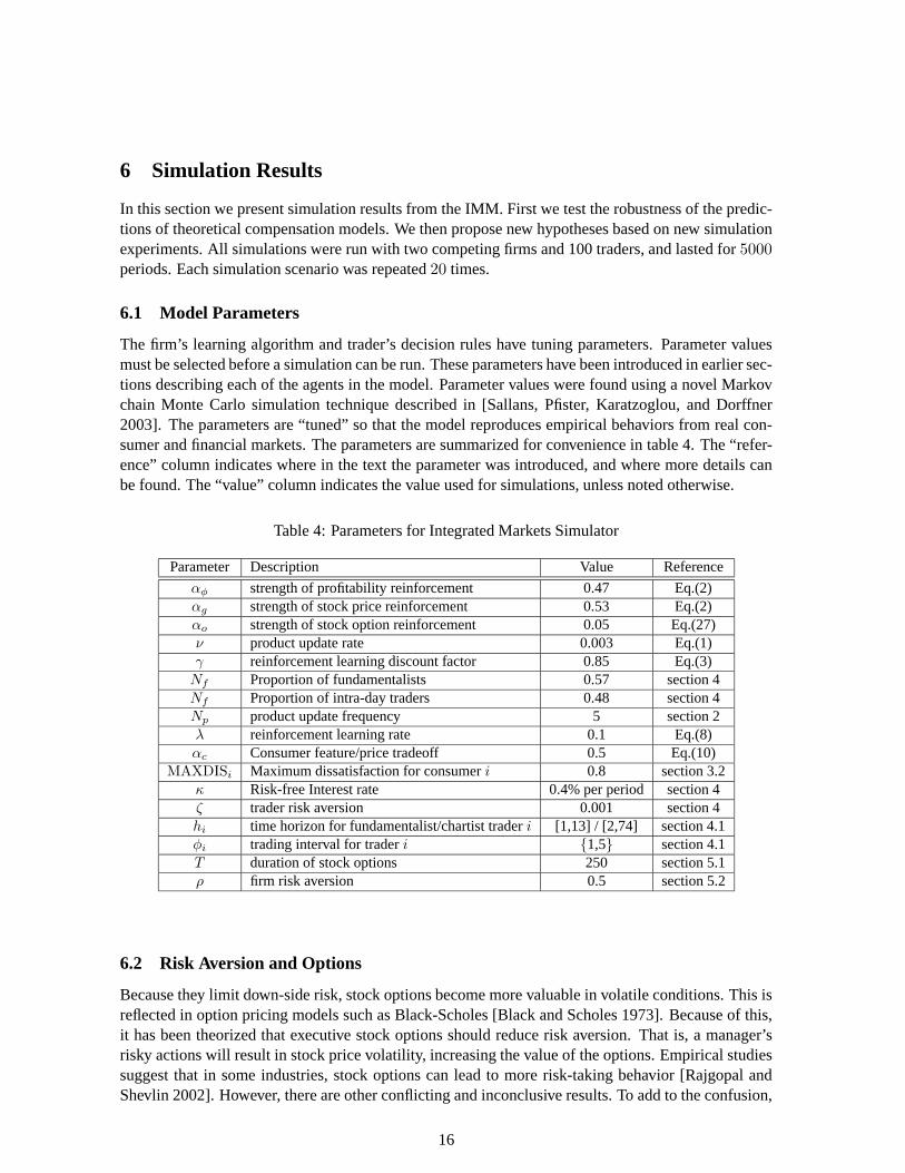
The firm’s learning algorithm and trader’s decision rules have tuning parameters. Parameter valuesmust be selected before a simulation can be run. These parameters have been introduced in earlier sec-tions describing each of the agents in the model. Parameter values were found using a novel Markovchain Monte Carlo simulation technique described in [Sallans, Pfister, Karatzoglou, and Dorffner2003]. The parameters are “tuned” so that the model reproduces empirical behaviors from real con-sumer and financial markets. The parameters are summarized for convenience in table 4. The “refer-ence” column indicates where in the text the parameter was introduced, and where more details canbe found. The “value” column indicates the value used for simulations, unless noted otherwise.

Table 4: Parameters for Integrated Markets Simulator

Parameter Description Value Reference

αφ strength of profitability reinforcement 0.47 Eq.(2)αg strength of stock price reinforcement 0.53 Eq.(2)αo strength of stock option reinforcement 0.05 Eq.(27)ν product update rate 0.003 Eq.(1)γ reinforcement learning discount factor 0.85 Eq.(3)

Nf Proportion of fundamentalists 0.57 section 4Nf Proportion of intra-day traders 0.48 section 4Np product update frequency 5 section 2λ reinforcement learning rate 0.1 Eq.(8)αc Consumer feature/price tradeoff 0.5 Eq.(10)

MAXDISi Maximum dissatisfaction for consumer i 0.8 section 3.2κ Risk-free Interest rate 0.4% per period section 4ζ trader risk aversion 0.001 section 4hi time horizon for fundamentalist/chartist trader i [1,13] / [2,74] section 4.1φi trading interval for trader i {1,5} section 4.1T duration of stock options 250 section 5.1ρ firm risk aversion 0.5 section 5.2

6.2 Risk Aversion and Options

Because they limit down-side risk, stock options become more valuable in volatile conditions. This isreflected in option pricing models such as Black-Scholes [Black and Scholes 1973]. Because of this,it has been theorized that executive stock options should reduce risk aversion. That is, a manager’srisky actions will result in stock price volatility, increasing the value of the options. Empirical studiessuggest that in some industries, stock options can lead to more risk-taking behavior [Rajgopal andShevlin 2002]. However, there are other conflicting and inconclusive results. To add to the confusion,

16

it is not entirely clear how executive options should be valued [Hall and Murphy 2002], or if thismechanism is even considered when awarding options. See Murphy [1999] for a review of executivecompensation.

In order to clarify whether stock options enhance risk-taking behavior, we simulated the use ofoptions with risk-neutral and risk-averse managers. We also used two different market conditions: onewhere the firms can quickly modify their products, and one where the products can only be modifiedslowly.

Our purpose for doing this simulation is twofold. First, it is unclear from empirical studies ofstock option usage if and when awarding options increases risk-taking. Theoretical models indicatethis should be the case. We will use the IMM as a test-bed to confirm this theory. There is noexplicit link between option value and risk-taking in our model, and the firm decision-making wasnot designed with this test in mind. The IMM therefore offers a good test of the robustness of theinfluence of stock options under conditions that are more realistic than the theoretical models: themanagers are uncertain, can suffer from misconceptions, and do not know with certainty the outcomeor riskiness of their actions. To our knowledge, this is the first attempt to validate the predictions ofprinciple-agency theory in a boundedly-rational, learning system.

Second, we would like to demonstrate that reinforcement learning is a good tool for modelinglearning and decision-making in the firm. If the behavior of the model matches theoretical predictions,then we can conclude that the managers are behaving rationally, within the bounds of their knowledge.This would indicate that reinforcement learning is a good alternative to evolutionary algorithms formodeling learning during the lifetime of a firm.

For each market condition we did three types of simulations: One with risk-neutral managers,one with risk-averse managers, and one with risk-averse managers with stock options. For the risk-averse managers, the risk aversion ρ = 0.5, and the strength of the stock option compensation wasαo = 0.05. The results, averaged over the 20 simulations, are shown in figure 3. For the options,the option duration was 250 periods; the option is granted slightly out of the money at 1.05 times thecurrent stock price; and the interest rate κ was 0.4% per period. For valuation purposes, the currentvariance of the stock was estimated over the last 10 periods. This short interval was chosen to decreasethe time lag between a variance-enhancing action and its subsequent effect on option value.

In both market conditions, the risk-averse managers have much worse performance, and lowervariance in their achieved profits. The effect of risk aversion is clearly reduced by adding stockoptions to the manager’s compensation. In the case of the slow-market condition, the average profitsachieved by the firm are equivalent to the risk-neutral case. The performance with stock options inthe fast-market condition is slightly inferior to the performance in the slow-market condition (thedifference is significant at the 5% level, according to a t-test).

The simulated stock options have the effect predicted by principal-agent theory. The behavior ofthe risk-averse manager leads to lower but more stable profits on average. The use of stock optionsboosts both expected profits and profit volatility. The effect of options is smaller in the fast marketcondition. This may simply be because the effect of product update actions is easier to estimate inthe slow market condition. When all actions have similar volatility, it requires fewer iterations to getan accurate estimate. This is because the dynamic programming algorithm uses information fromfuture actions to estimate the volatility of current actions. An inaccurate estimate of action volatilityresults in inaccurate action selection, and lower profits during learning. The performance with nostock options (in the risk-averse case) is also slightly inferior in the fast market condition to the slowmarket condition (the difference is significant at the 5% level, according to a t-test). We show thedifference in action volatility in the two conditions in figure 4).

What does this mean to real markets? The benefit of stock options depends on being able to

17

NSN ASN ASO NFN AFN AFO0

100

200

300

400

500

600

700

800

900

Mea

n P

rofit

Simulation

Figure 3: The effect of stock options on risk aversion. Mean and standard error of per-time-step profitsare shown for six conditions: N??==risk neutral, A??==risk averse; ?S?==slow product movement,?F?==fast product movement; ??N==no stock options, ??O==stock options. The risk-averse managerscause mean profits to drop, and the variance of the profits to be reduced. In the slow market case,options boost expected profits and profit volatility. In the fast market conditions, the options alsoboost profits, but not as much as in the slow market case.

1 2 3 4 5 6 7 8 9 103

3.5

4

4.5

5

5.5

6

6.5

7

action

com

pens

atio

n vo

latil

ity

Slow Market

1 2 3 4 5 6 7 8 9 103

3.5

4

4.5

5

5.5

6

6.5

7

action

com

pens

atio

n vo

latil

ity

Fast Market

Figure 4: The manager’s average estimate of standard error for each potential action in the a) slow-moving consumer market and b) fast-moving consumer market. The actions are: 1. Take a randomaction from the remaining actions. 2. Do nothing. 3. Increase product price by 1. 4. Decrease productprice by 1. 5-10. Modify product attributes.

correctly identify high-risk actions. If the manager is not able to accurately estimate how risky anaction is, the benefit of stock options will be muted.

Notice a byproduct of this simulation: In a competitive market with price-sensitive consumers,raising prices is very risky. In the fast-moving market, doing nothing actually becomes a safer bet(has lower variance) than in the slow-moving market. Lowering prices is always safe.

18

These simulations also validate the choice of reinforcement learning to model learning and decision-making in the firm. Using this technique managers are able to estimate the value and the volatilityof their actions. The managers act rationally, within the bounds of their knowledge. Reinforcementlearning offers a good technique for modeling learning in the firm.

6.3 Market Competition and Options

In this section we model a scenario which is difficult to address with an analytic model: How stockoptions influence the performance of a new competitor entering a market dominated by an incumbentfirm. The incumbent has the benefit of prior experience in the market. This could also be seen as adisadvantage: The competitor does not have to overcome old habits that are no longer valid in the newcompetitive environment.

Hypothesis 1: The incumbent will have an inherent advantage because of its prior knowledge of themarket.

Hypothesis 2: Options will help the incumbent, because they will promote exploration.

Hypothesis 3: Options will help the entrant for the same reason.

Here “exploration” means trying new products or pricing strategies, in order to learn whetheror not they work. Exploration is inherently a risky action, because it sacrifices current profits in anattempt to boost future profits. Knowledge acquisition by the manager is a crucial consideration inany realistic model of firm behavior.

We modeled four scenarios: The incumbent and entrant have no stock options; the entrant receivesstock options with the incumbent having none; and two scenarios where both receive options. In theselast two scenarios, the incumbent receives its options either from the start of the simulation, or whenthe new entrant arrives. All managers are risk averse, and all simulations run for 5000 iterations. Theentrant enters the market at iteration 2000 (see figure 5).

Given no options, the incumbent on average does better than the new entrant (significant at the 1%level according to a t-test). These results support hypothesis 1. The results also support hypothesis 2:When the entrant is granted options, it does as well as the incumbent. Note that the incumbent nowdoes less well because of competition from the entrant. The results for hypothesis 3 are mixed. Whenoptions are granted to the incumbent at the beginning of the simulation, it does no better than whenit had no options (i.e. the result is not significant according to a t-test). However, when options aregranted only after the new entrant appears, it does better on average than without options (significantat the 5% level according to a t-test).

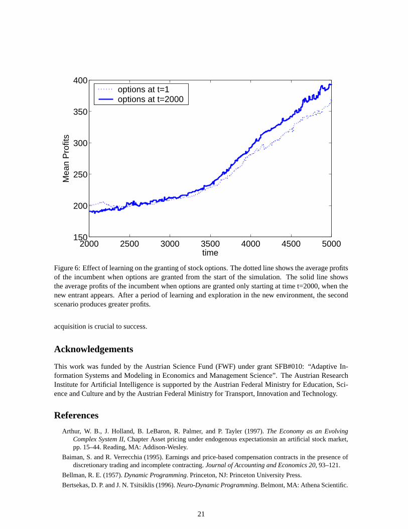
This suggests that encouraging risk-taking is not enough, but rather the incumbent manager needsto be encouraged to take risks specifically after the new threat appears. This is followed by a periodof new exploration and learning, which results in the higher profits. Figure 6 shows average profitsversus time for the incumbent firm for the last two stock options conditions. Initially, there is nodifference in performance between the two. It is only after some learning and exploration time thatthe performance difference is seen.

We can therefore make a new prediction to be tested using empirical data: While options will helpa new entrant be competitive in a new market, they will be most effective in helping the incumbentwhen they are granted after the new entrant appears. This suggests that re-examination of compensa-tion is particularly important when a firm is facing new competition. Encouraging risk-taking at thistime can be particularly helpful.

19

NO OPT ENT OPT BOTH OPT BOTH OPT 2000150

200

250

300

350

400

450

Mea

n P

rofit

s

Option Grants

IncumbentEntrant

Figure 5: Results of a new entrant in the market. The bar graphs show the average per-time-step profitsand standard errors for four scenarios: no stock options (NO OPT); an entrant firm with options (ENTOPT); both with options (BOTH OPT); and both with options, where the incumbent firm has optionsgranted at the time the new entrant arrives (time t=2000) (BOTH OPT 2000). The incumbent is black,and the new entrant is white. The new entrant was always granted stock options from time t=1. Theaverages were taken over the time from the arrival of the new entrant (time t=2000) to the end ofthe simulation (time t=5000). Options granted to the entrant help it to compete with the incumbent.Options helped the incumbent when they were granted at the time that the new entrant arrived.

7 Conclusions

In this article we have presented a computational economics model of managerial compensation. Wehave simulated risk-averse managers with and without stock-option compensation, and shown that thecomputational model confirms the predictions of principal agency theory. In particular, stock optionsencourage risk taking in otherwise risk-averse managers, and can boost overall profits by encouragingexploration. In addition, we show that these effects are quite robust, occurring in our model in thepresence of learning and incomplete knowledge. As a byproduct, we show that reinforcement learningoffers a valuable alternative for modeling learning and decision-making in economic agents. Webelieve that it is a better model of learning within the lifetime of a process than alternatives such asgenetic algorithms.

We simulate the scenario of a new entrant challenging an incumbent firm. We show that stockoptions can boost the competitiveness of the entrant, and also help the incumbent to fight off com-petition. In the latter case, the options are most effective when they are introduced as a response tothe new competition, boosting exploration and learning in the new competitive environment. Thissuggests that it is particularly important to revisit compensation contracts, introducing risk-taking in-centives, when the state of competition in the market changes. It also suggests that empirical researchinto the effectiveness of stock options should take the experience of the manager and age of the firminto account. In our simulations, options are most effective in the situation where new knowledge

20

2000 2500 3000 3500 4000 4500 5000150

200

250

300

350

400

time

Mea

n P

rofit

s

options at t=1options at t=2000

Figure 6: Effect of learning on the granting of stock options. The dotted line shows the average profitsof the incumbent when options are granted from the start of the simulation. The solid line showsthe average profits of the incumbent when options are granted only starting at time t=2000, when thenew entrant appears. After a period of learning and exploration in the new environment, the secondscenario produces greater profits.

acquisition is crucial to success.

Acknowledgements

This work was funded by the Austrian Science Fund (FWF) under grant SFB#010: “Adaptive In-formation Systems and Modeling in Economics and Management Science”. The Austrian ResearchInstitute for Artificial Intelligence is supported by the Austrian Federal Ministry for Education, Sci-ence and Culture and by the Austrian Federal Ministry for Transport, Innovation and Technology.

References

Arthur, W. B., J. Holland, B. LeBaron, R. Palmer, and P. Tayler (1997). The Economy as an EvolvingComplex System II, Chapter Asset pricing under endogenous expectationsin an artificial stock market,pp. 15–44. Reading, MA: Addison-Wesley.

Baiman, S. and R. Verrecchia (1995). Earnings and price-based compensation contracts in the presence ofdiscretionary trading and incomplete contracting. Journal of Accounting and Economics 20, 93–121.

Bellman, R. E. (1957). Dynamic Programming. Princeton, NJ: Princeton University Press.

Bertsekas, D. P. and J. N. Tsitsiklis (1996). Neuro-Dynamic Programming. Belmont, MA: Athena Scientific.

21

Black, F. and M. Scholes (1973). The pricing of options and corporate liabilities. Journal of Political Econ-omy 81, 637–654.

Brock, W. and C. Hommes (1997). A rational route to randomness. Econometrica 65, 1059–1095.

Brock, W. and C. Hommes (1998). Heterogeneous beliefs and routes to chaos in a simple asset pricingmodel. Journal of Economic Dynamics and Control 22, 1235–1274.

Bushman, R. and R. Indjejikian (1993). Accounting income, stock price and managerial compensation.Journal of Accounting and Economics 16, 3–24.

Chiarella, C. and X. He (2001). Asset pricing and wealth dynamics under heterogeneous expectations. Quan-titative Finance 1, 509–526.

Chiarella, C. and X. He (2002). Heterogeneous beliefs, risk and learning in a simple asset pricing model.Computational Economics 19, 95–132.

Choe, C. (1998). A mechanism design approach to an optimal contract under ex ante and ex post privateinformation. Review of Economic Design 3(3), 237–255.

Dangl, T., E. Dockner, A. Gaunersdorfer, A. Pfister, A. Soegner, and G. Strobl (2001). Adaptive erwartungs-bildung und finanzmarktdynamik. Zeitschrift fur betriebswirtschaftliche Forschung 53, 339–365.

Grossman, S. (1989). The Informational Role of Prices. Cambridge, MA: MIT Press.

Hall, B. J. and K. J. Murphy (2002). Stock options for undiversified executives. Journal of Accounting andEconomics 33, 3–42.

Holmstrom, B. (1979). Moral hazard and observability. Bell Journal of Economics 10, 74–91.

Jaakkola, T. S., S. P. Singh, and M. I. Jordan (1995). Reinforcement learning algorithm for partially observ-able Markov decision problems. In G. Tesauro, D. S. Touretzky, and T. K. Leen (Eds.), Advances inNeural Information Processing Systems, Volume 7, pp. 345–352. The MIT Press, Cambridge.

Levy, M. and H. Levy (1996). The danger of assuming homogeneous expectations. Financial AnalysistsJournal 52(3), 65–70.

Murphy, K. J. (1999). Handbook of Labor Economics, Volume 3, Chapter Executive Compensation. Ams-terdam: North Holland.

Pfister, A. (2003). Heterogeneous trade intervals in an agent based financial market. Technical report, SFBAdaptive Information Systems and Modelling in Economics and Management Science.

Rajgopal, S. and T. J. Shevlin (2002). Empirical evidence on the relation between stock option compensationand risk taking. Journal of Accounting and Economics 33(2).

Rummery, G. A. and M. Niranjan (1994). On-line Q-learning using connectionist systems. Technical ReportCUED/F-INFENG/TR 166, Engineering Department, Cambridge University.

Sallans, B., G. Dorffner, and A. Karatzoglou (2002). Feedback effects in interacting markets. In C. Urban(Ed.), Proceedings of the Third Workshop on Agent-Based Simulation, pp. 126–131. SCS-EuropeanPublishing House, Ghent, Belgium.

Sallans, B., A. Pfister, A. Karatzoglou, and G. Dorffner (2003). Simulation and validation of an integratedmarkets model. Journal of Artificial Societies and Social Simulation 6(4).

Simon, H. A. (1982). Models of Bounded Rationality, Vol 2: Behavioral Economics and Business Organiza-tion. Cambridge, MA: The MIT Press.

Sutton, R. S. (1996). Generalization in reinforcement learning: Successful examples using sparse coarsecoding. In D. S. Touretzky, M. C. Mozer, and M. E. Hasselmo (Eds.), Advances in Neural InformationProcessing Systems, Volume 8, pp. 1038–1044. The MIT Press, Cambridge.

Sutton, R. S. and A. G. Barto (1998). Reinforcement Learning: An Introduction. Cambridge, MA: The MITPress.

Tesauro, G. (1999). Pricing in agent economies using neural networks and multi-agent Q-learning. In IJCAI-99.

Tesfatsion, L. (2002). Agent-based computational economics: Growing economies from the bottom up.Artificial Life 8(1), 55–82.

22

Watkins, C. J. C. H. (1989). Learning from Delayed Rewards. Cambridge, UK: Cambridge University. Ph.D.thesis.

Watkins, C. J. C. H. and P. Dayan (1992). Q-learning. Machine Learning 8, 279–292.

23