A Simulation Strategy to Ensure Pipeline Integrity · PDF fileA Simulation Strategy to Ensure...

5th Pipeline Technology Conference 2010

A Simulation Strategy to Ensure Pipeline Integrity

F. Van den Abeele and P. Thibaux ArcelorMittal Global R&D Gent (OCAS N.V.)

J.F. Kennedylaan 3, BE-9060 Zelzate, Belgium

ABSTRACT The ability to arrest a running crack is one of the key features in the safe design of pipeline systems. In the current design codes, the crack arrest properties of a pipeline should meet two requirements: crack propagation has to occur in a ductile fashion, and enough energy should be dissipated during propagation. While the first criterion is assessed by the Battelle Drop Weight Tear Test (BDWTT) at low temperatures, the latter requirement is converted into a lower bound for the impact energy absorbed during a Charpy test. This required minimum value for impact energy is function of the steel grade, the internal pressure and the diameter of the pipe. For X70 and X80 API grades, the typical range of 50 – 120 J was determined empirically by comparing lab-scale toughness tests with full-scale burst tests. Higher strength materials (X100 and beyond) have revealed that the commonly used relations no longer hold, hence further understanding of the material is required to ensure the safe operation of a pipeline. Several approaches have been proposed to characterize the toughness of linepipe steels, in an attempt to resolve the shortcomings of the Charpy V-notch impact test. A lot of attention is drawn to local toughness measures like crack tip opening angle (CTOA). However, it is not straightforward to transfer these descriptions between specimen of different thicknesses or geometry, as the influence of stress triaxiality does not correspond to local physical processes like void growth and coalescence. Numerical models with a local damage description are potentially able to predict the failure of a material for different geometries and thicknesses. These models are based on the computation of void growth according to Rice and Tracey, and account for the local softening of the material due to void nucleation, growth and subsequent coalescence. The Gurson-Tvergaard-Needleman (GTN) model is commonly used in computational fracture mechanics, e.g. to simulate the Charpy V-notch impact test. In this paper, a simulation strategy to ensure pipeline integrity is proposed. Computational fracture mechanics methods are presented to acquire a more profound understanding of toughness requirements and ductile crack propagation in pipeline steels. The ability of current computer codes to estimate J-integrals is demonstrated by the simulation of compact tension tests. Then, the Gurson-Tvergaard-Needleman damage model is applied to predict crack propagation during Charpy impact experiments, where notched tensile tests were performed to calibrate the material model parameters. In addition, a brief review of cohesive zone models is presented to simulate crack propagation and arrest in high pressure gas pipelines. Case studies on composite crack arrestors and mitigation measures to address vortex induced vibrations will endorse the merits of finite element analysis in pipeline design.


1. THE MERITS AND LIMITS OF COMPUTATIONAL FRACTURE MECHANICS The finite element method is a numerical technique that can be used for the solution of complex engineering problems [01-03]. The concept is simply based on replacing the partial differential equations, describing the physical problem, by a system of simultaneous algebraic equations (for steady state problems) or a set of ordinary differential equations (for time dependent problems). This can be achieved in two essential steps: (i) writing the variational equivalent or weak form of the partial differential equation (ii) reducing the problem size to finite space dimensions through discretization The finite element method was developed more than 50 years ago for the civil engineering and aircraft industry, but the potential of the method to solve different types of applied science and engineering problems was recognized soon. In the mean time, finite element analysis is a well established numerical tool to tackle a wide range of practical problems. However, while design engineers already rely on finite element methods to predict manufacturing processes, structural stiffness and strength, heat transfer, vibroacoustics etc, pipeline engineering is still based on experimental (and often large-scale) testing and empirical proof of concept. Most pipe designers are reluctant to accept the merits that numerical methods can bring. In this paper, a simulation strategy to ensure pipeline integrity is proposed. The added value of numerical modelling is demonstrated for different stages during the pipeline design and operation:

• Computational fracture mechanics methods [04-05] are presented to acquire a more profound understanding of toughness requirements and ductile crack propagation in pipeline steels.

• A numerical scheme is introduced to predict the evolution of mechanical

properties during the production process of a pipe. Based on merely uniaxial test data on coil, the properties of the manufacture pipe can be estimated.

• Finite element analysis can assist in the safe design of pipeline systems. A

case study on composite crack arrestors is included to show the tangible contribution of numerical methods to fracture propagation control and pipeline integrity.

• Multiphysics modelling is applied to calculate complex flow patterns around

submarine pipelines. Coupled solvers can calculate fluid-structure interactions and predict vortex induced vibrations in offshore pipeline spans. A parametric numerical model allows evaluating different mitigation measures.

Each time, the numerical simulations are endorsed by experimental results. The combined approach, presented in this paper, is considered the most efficient and economic strategy to ensure pipeline integrity.


2. TOUGHNESS MODELLING OF MODERN PIPELINE STEELS The occurence of a longitudinal crack propagating along a gas pipeline is a catastrophic event, which involves both economic losses and environmental damage. For this reason, fracture propagation control is of major importance when designing gas pipelines to be operated at high pressures. While brittle fracture is typically achieved by ensuring that the pipeline is operated well above the Ductile to Brittle Transition Temperature, the ductile fracture propagation control can be avoided (or at least limited) by increasing the minimum specified toughness of the linepipe steel. ArcelorMittal, the world’s leading steel company, delivers hot rolled products from coil to serve the demanding oil and gas industry. The ArcelorMittal hot strip mills are equipped with heavy downcoilers, allowing the production of heavy gauge X70 and X80 pipeline steel grades. A comprehensive review on these recent developments of high strength linepipe steels on coil is presented in [06]. The opportunity for the dimensional enlargement of spiral welded pipes by offering X70 and X80 on coil with thickness up to 25 mm is discussed in [07], with specific attention to low temperature toughness. Investigations on the weld properties of High Frequency Induction (HFI) welded pipes are reported in [08], and the link between the microstructure and the toughness will be presented in [09]. In addition, ArcelorMittal is developing heavy gauge high strength pipeline steel (X80, 22 mm) and ultra-high strength steel (X100) on coil as well [10-11]. However, for such ultra high grades, the identification of a reliable crack propagation strategy is no longer straightforward. Indeed, despite excellent toughness values at lab scale (Charpy upper shelf energy and Battelle shear fracture area), one can no longer rely on pipe body arrest [12-14]. Computational fracture mechanics provides a means of assessing the traditional fracture mechanics tests, and sheds a brighter light on the material resistance to ductile crack propagation during such experiments. In this section, the Gurson-Tvergaard-Needleman (GTN) damage model to simulate ductile failure is presented. The model parameters are tuned by comparing finite element simulations with notched tensile tests for different values for triaxiality. The calibrated damage model is applied to calculate J-integrals and predict crack growth in compact tension tests. Moreover, the finite element analysis, presented here, reveals important features on the energy dissipation during Charpy V-notch impact experiments. 2.1 Notched Tensile Tests to Calibrate the Gurson Damage Parameters

Several approaches can be pursued to model plastic deformation and ductile failure of metals. Cohesive zone models (cfr. section 4), for instance, idealize the fracture process in solids as occurring within thin layers confined by two adjacent virtual surfaces [15-16]. The introduction of a constitutive law on the interface, connecting tractions and displacements, provides a phenomeno-logical description for the progressive fracture in ductile metals. Indeed, the loss of cohesion –and thus crack nucleation and propagation- can be viewed as the progressive decay of tension and shear stresses across the adjacent surfaces. Bonora [17-18] developed a continuum damage mechanics (CDM) model, where the growth of microvoids results in non linear damage accumulation with plastic deformation.


In this study at hand, we will apply the Gurson-Tvergaard-Needleman model, which is commonly used to model ductile failure in porous metals, driven by subsequent nucleation, growth and coalescence of voids. For metals containing a dilute concentration of voids, Gurson [19] proposed a yield condition

( )2

232 cosh 1 02y y

q pf fσ σ

Φ = + − − + =

(01)

where q is the effective von Mises stress, p is the hydrostatic pressure, σy is the yield stress of the fully dense matrix (as a function of the equivalent plastic strain), and the void volume fraction

void

matrix

VfV

= (02)

is the ratio of the volume of voids Vvoid to the total matrix volume Vmatrix. The change in void volume fraction

( )1 :plf f Iε= −& & (03) is governed by the growth of the existing voids, and based on the conservation of mass. To improve the model predictions for periodic arrays of cylindrical and spherical voids, Tvergaard [20-21] introduced three parameters q1, q2 and q3:

( )2

21 2 3

32 cosh 1 02y y

q pq f q q fσ σ

Φ = + − − + =

(04)

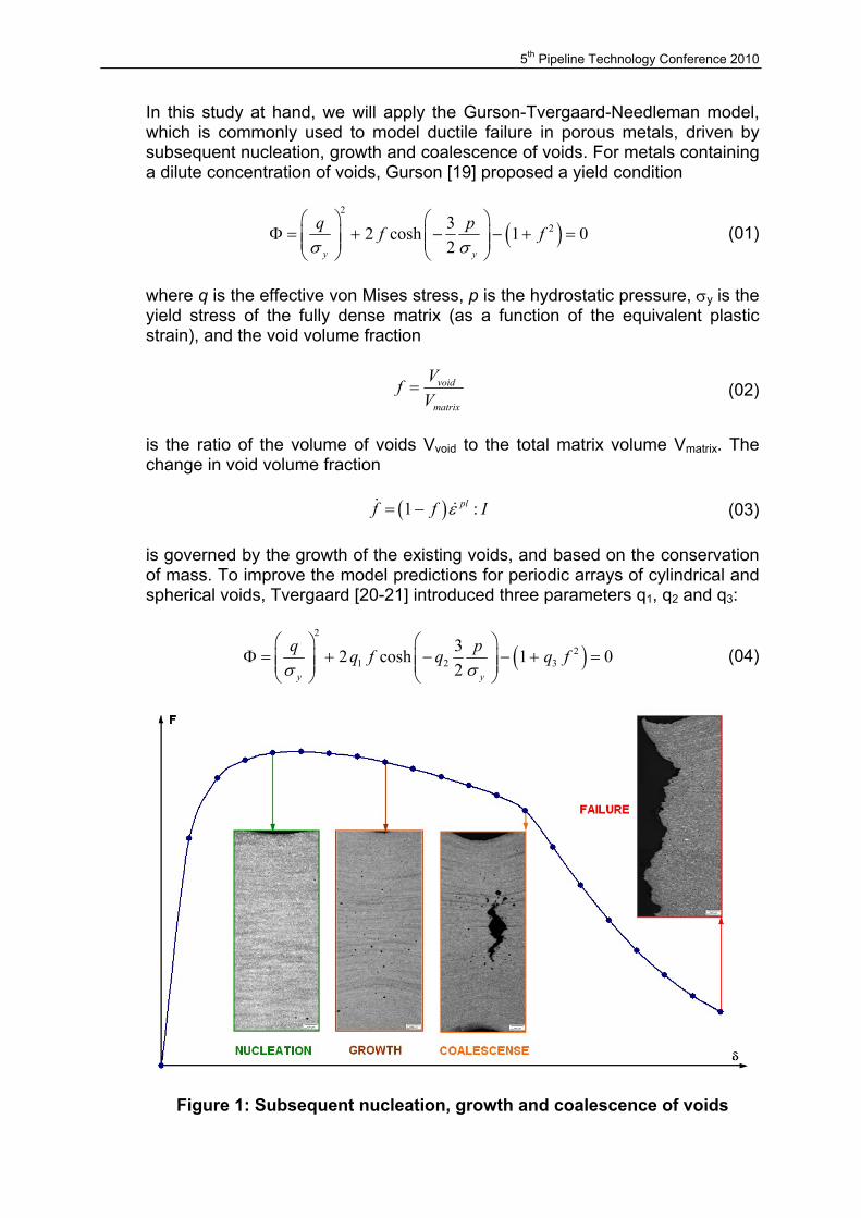
Figure 1: Subsequent nucleation, growth and coalescence of voids


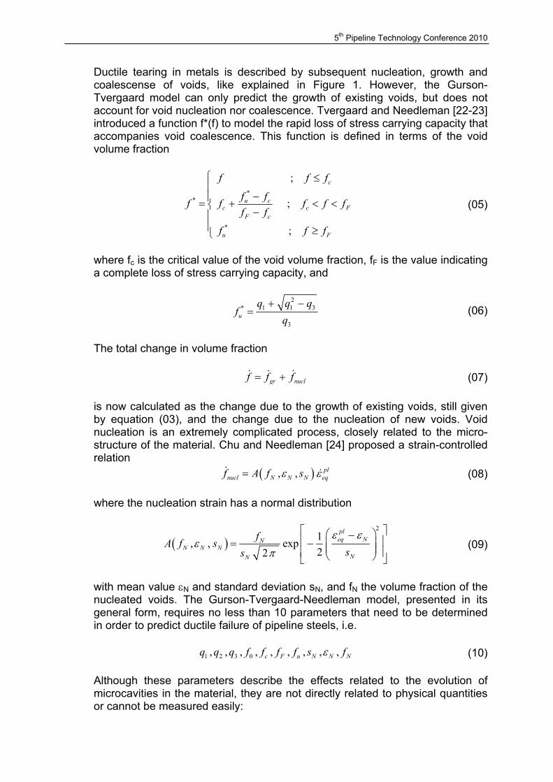
Ductile tearing in metals is described by subsequent nucleation, growth and coalescense of voids, like explained in Figure 1. However, the Gurson-Tvergaard model can only predict the growth of existing voids, but does not account for void nucleation nor coalescence. Tvergaard and Needleman [22-23] introduced a function f*(f) to model the rapid loss of stress carrying capacity that accompanies void coalescence. This function is defined in terms of the void volume fraction

**

*

;

;

;

c

u cc c F

F c

u F

f f f

f ff f f f ff f

f f f

≤

−= + < < − ≥

(05)

where fc is the critical value of the void volume fraction, fF is the value indicating a complete loss of stress carrying capacity, and

21 1 3*

3u

q q qf

q+ −

= (06)

The total change in volume fraction

gr nuclf f f= +& & & (07) is now calculated as the change due to the growth of existing voids, still given by equation (03), and the change due to the nucleation of new voids. Void nucleation is an extremely complicated process, closely related to the micro-structure of the material. Chu and Needleman [24] proposed a strain-controlled relation

( ), , plnucl N N N eqf A f sε ε=& & (08)

where the nucleation strain has a normal distribution

( )2

1, , exp22

pleq NN

N N NNN

fA f sss

ε εε

π

− = −

(09)

with mean value εN and standard deviation sN, and fN the volume fraction of the nucleated voids. The Gurson-Tvergaard-Needleman model, presented in its general form, requires no less than 10 parameters that need to be determined in order to predict ductile failure of pipeline steels, i.e.

1 2 3 0, , , , , , , , ,c F u N N Nq q q f f f f s fε (10) Although these parameters describe the effects related to the evolution of microcavities in the material, they are not directly related to physical quantities or cannot be measured easily:


• The first three parameters q1, q2 and q3 determine the evolution of the yielding function, together with the triaxiality and porosity

• The four parameters f0, fc, fF and fu determine the porosity evolution law • The remaining three parameters sN, εN and fN describe the nucleation of

new voids

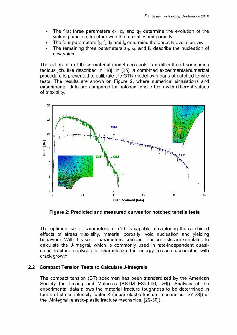
The calibration of these material model constants is a difficult and sometimes tedious job, like described in [18]. In [25], a combined experimental/numerical procedure is presented to calibrate the GTN model by means of notched tensile tests. The results are shown on Figure 2, where numerical simulations and experimental data are compared for notched tensile tests with different values of triaxiality.

Figure 2: Predicted and measured curves for notched tensile tests

The optimum set of parameters for (10) is capable of capturing the combined effects of stress triaxiality, material porosity, void nucleation and yielding behaviour. With this set of parameters, compact tension tests are simulated to calculate the J-integral, which is commonly used in rate-independent quasi-static fracture analyses to characterize the energy release associated with crack growth.

2.2 Compact Tension Tests to Calculate J-Integrals

The compact tension (CT) specimen has been standardized by the American Society for Testing and Materials (ASTM E399-90, [26]). Analysis of the experimental data allows the material fracture toughness to be determined in terms of stress intensity factor K (linear elastic fracture mechanics, [27-28]) or the J-integral (elastic-plastic fracture mechanics, [29-30]).


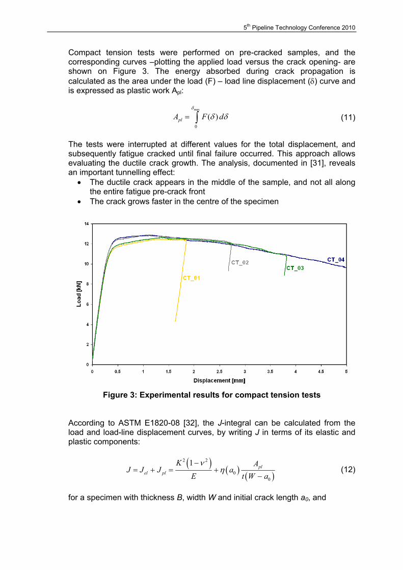
Compact tension tests were performed on pre-cracked samples, and the corresponding curves –plotting the applied load versus the crack opening- are shown on Figure 3. The energy absorbed during crack propagation is calculated as the area under the load (F) – load line displacement (δ) curve and is expressed as plastic work Apl:

max

0

( )plA F dδ

δ δ= ∫ (11)

The tests were interrupted at different values for the total displacement, and subsequently fatigue cracked until final failure occurred. This approach allows evaluating the ductile crack growth. The analysis, documented in [31], reveals an important tunnelling effect:

• The ductile crack appears in the middle of the sample, and not all along the entire fatigue pre-crack front

• The crack grows faster in the centre of the specimen

Figure 3: Experimental results for compact tension tests

According to ASTM E1820-08 [32], the J-integral can be calculated from the load and load-line displacement curves, by writing J in terms of its elastic and plastic components:

( ) ( ) ( )

2 2

00

1 plel pl

K AJ J J a

E t W a

νη

−= + = +

− (12)

for a specimen with thickness B, width W and initial crack length a0, and


0aPK fWB W = &

(13)

where P is the load on the specimen. For a compact tension specimen [32], the constraint factor is

( ) 00 2 0.522W aa

Wη −

= + (14)

and 2

0 00

03 3 42

0 00

0.886 4.64 13.322

14.72 5.601

a aaW Wa Wf

W a aaW W W

+ − + = + −−

(15)

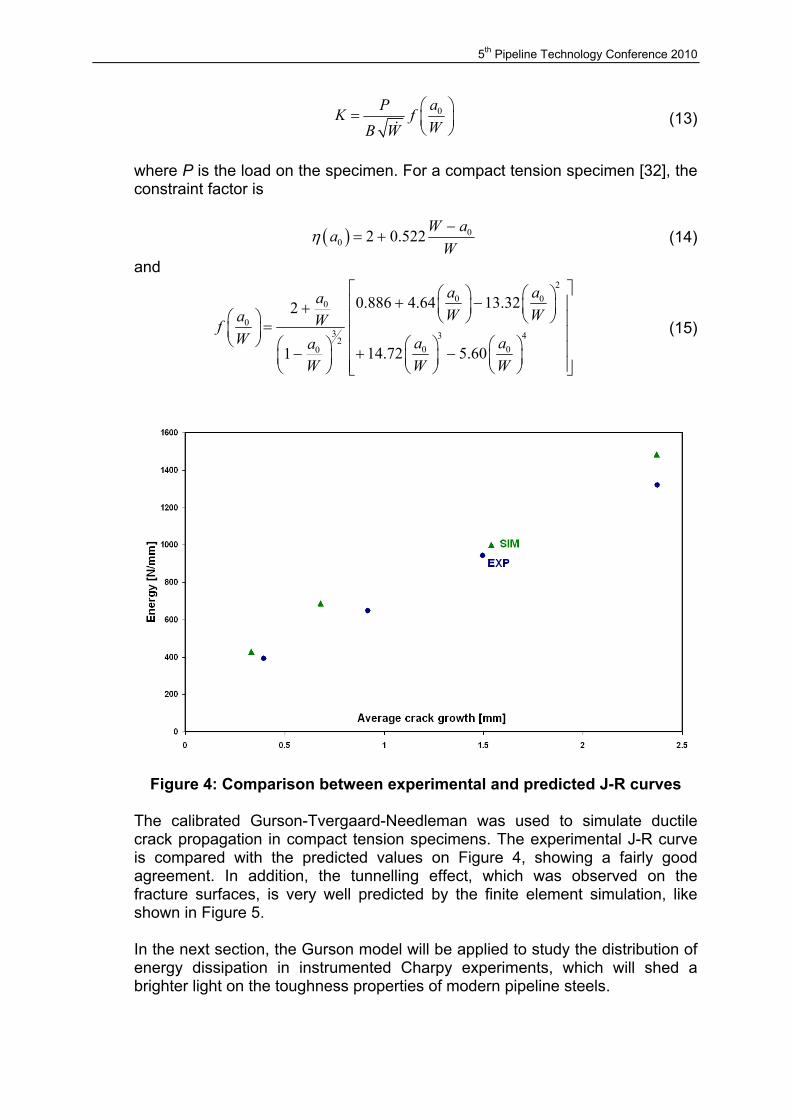
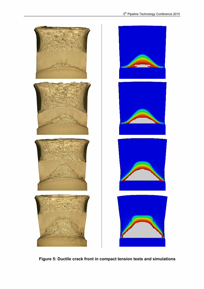
Figure 4: Comparison between experimental and predicted J-R curves The calibrated Gurson-Tvergaard-Needleman was used to simulate ductile crack propagation in compact tension specimens. The experimental J-R curve is compared with the predicted values on Figure 4, showing a fairly good agreement. In addition, the tunnelling effect, which was observed on the fracture surfaces, is very well predicted by the finite element simulation, like shown in Figure 5. In the next section, the Gurson model will be applied to study the distribution of energy dissipation in instrumented Charpy experiments, which will shed a brighter light on the toughness properties of modern pipeline steels.


Figure 5: Ductile crack front in compact tension tests and simulations


. 2.3 Charpy Impact Experiments to Predict Toughness of Pipeline Steels

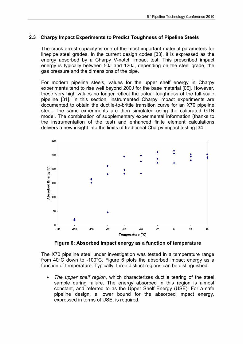
The crack arrest capacity is one of the most important material parameters for linepipe steel grades. In the current design codes [33], it is expressed as the energy absorbed by a Charpy V-notch impact test. This prescribed impact energy is typically between 50J and 120J, depending on the steel grade, the gas pressure and the dimensions of the pipe. For modern pipeline steels, values for the upper shelf energy in Charpy experiments tend to rise well beyond 200J for the base material [06]. However, these very high values no longer reflect the actual toughness of the full-scale pipeline [31]. In this section, instrumented Charpy impact experiments are documented to obtain the ductile-to-brittle transition curve for an X70 pipeline steel. The same experiments are then simulated using the calibrated GTN model. The combination of supplementary experimental information (thanks to the instrumentation of the test) and enhanced finite element calculations delivers a new insight into the limits of traditional Charpy impact testing [34].

Figure 6: Absorbed impact energy as a function of temperature

The X70 pipeline steel under investigation was tested in a temperature range from 40°C down to -100°C. Figure 6 plots the absorbed impact energy as a function of temperature. Typically, three distinct regions can be distinguished:

• The upper shelf region, which characterizes ductile tearing of the steel

sample during failure. The energy absorbed in this region is almost constant, and referred to as the Upper Shelf Energy (USE). For a safe pipeline design, a lower bound for the absorbed impact energy, expressed in terms of USE, is required.


• The lower shelf region. The energy values in this region are typically an order of magnitude lower than in the upper shelf region, hence reflecting brittle fracture of the steel sample at lower temperatures.

• The transition region. Between both levels of energy, there is a transition

region where the final failure is a combination of both ductile and brittle behaviour. In this region, a large scatter in energy values is usually obtained. The Ductile to Brittle Transition Temperature (DBTT) can be calculated in different ways [35], and is commonly used to distinguish between ductile failure and brittle fracture. Hence, this DBTT is an important parameter in the safe design of pipelines.

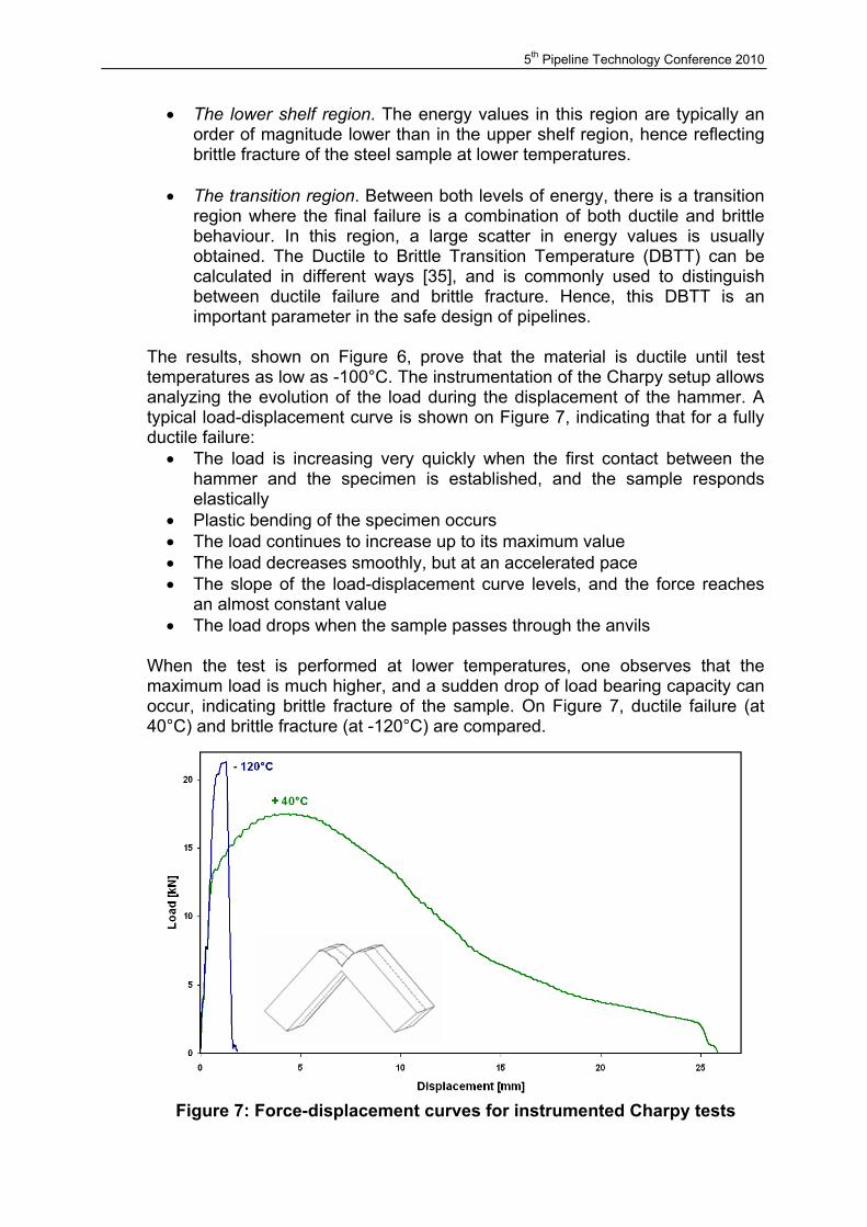
The results, shown on Figure 6, prove that the material is ductile until test temperatures as low as -100°C. The instrumentation of the Charpy setup allows analyzing the evolution of the load during the displacement of the hammer. A typical load-displacement curve is shown on Figure 7, indicating that for a fully ductile failure:

• The load is increasing very quickly when the first contact between the hammer and the specimen is established, and the sample responds elastically

• Plastic bending of the specimen occurs • The load continues to increase up to its maximum value • The load decreases smoothly, but at an accelerated pace • The slope of the load-displacement curve levels, and the force reaches

an almost constant value • The load drops when the sample passes through the anvils

When the test is performed at lower temperatures, one observes that the maximum load is much higher, and a sudden drop of load bearing capacity can occur, indicating brittle fracture of the sample. On Figure 7, ductile failure (at 40°C) and brittle fracture (at -120°C) are compared.

Figure 7: Force-displacement curves for instrumented Charpy tests


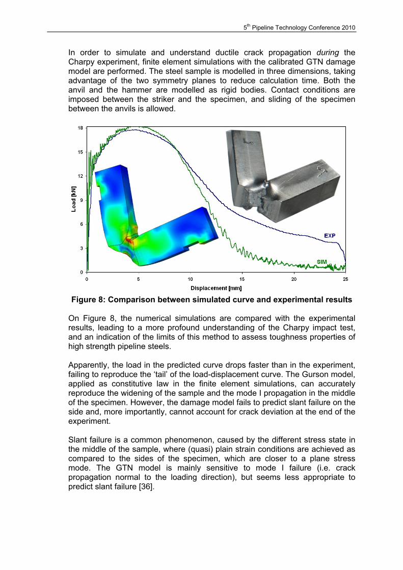
In order to simulate and understand ductile crack propagation during the Charpy experiment, finite element simulations with the calibrated GTN damage model are performed. The steel sample is modelled in three dimensions, taking advantage of the two symmetry planes to reduce calculation time. Both the anvil and the hammer are modelled as rigid bodies. Contact conditions are imposed between the striker and the specimen, and sliding of the specimen between the anvils is allowed.

Figure 8: Comparison between simulated curve and experimental results

On Figure 8, the numerical simulations are compared with the experimental results, leading to a more profound understanding of the Charpy impact test, and an indication of the limits of this method to assess toughness properties of high strength pipeline steels. Apparently, the load in the predicted curve drops faster than in the experiment, failing to reproduce the ‘tail’ of the load-displacement curve. The Gurson model, applied as constitutive law in the finite element simulations, can accurately reproduce the widening of the sample and the mode I propagation in the middle of the specimen. However, the damage model fails to predict slant failure on the side and, more importantly, cannot account for crack deviation at the end of the experiment. Slant failure is a common phenomenon, caused by the different stress state in the middle of the sample, where (quasi) plain strain conditions are achieved as compared to the sides of the specimen, which are closer to a plane stress mode. The GTN model is mainly sensitive to mode I failure (i.e. crack propagation normal to the loading direction), but seems less appropriate to predict slant failure [36].


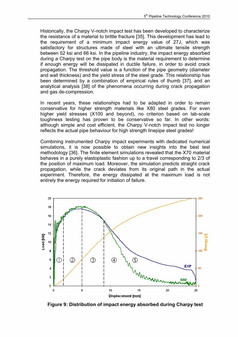
Historically, the Charpy V-notch impact test has been developed to characterize the resistance of a material to brittle fracture [35]. This development has lead to the requirement of a minimum impact energy value of 27J, which was satisfactory for structures made of steel with an ultimate tensile strength between 52 ksi and 66 ksi. In the pipeline industry, the impact energy absorbed during a Charpy test on the pipe body is the material requirement to determine if enough energy will be dissipated in ductile failure, in order to avoid crack propagation. The threshold value is a function of the pipe geometry (diameter and wall thickness) and the yield stress of the steel grade. This relationship has been determined by a combination of empirical rules of thumb [37], and an analytical analysis [38] of the phenomena occurring during crack propagation and gas de-compression. In recent years, these relationships had to be adapted in order to remain conservative for higher strength materials like X80 steel grades. For even higher yield stresses (X100 and beyond), no criterion based on lab-scale toughness testing has proven to be conservative so far. In other words: although simple and cost efficient, the Charpy V-notch impact test no longer reflects the actual pipe behaviour for high strength linepipe steel grades! Combining instrumented Charpy impact experiments with dedicated numerical simulations, it is now possible to obtain new insights into the best test methodology [36]. The finite element simulations revealed that the X70 material behaves in a purely elastoplastic fashion up to a travel corresponding to 2/3 of the position of maximum load. Moreover, the simulation predicts straight crack propagation, while the crack deviates from its original path in the actual experiment. Therefore, the energy dissipated at the maximum load is not entirely the energy required for initiation of failure.

Figure 9: Distribution of impact energy absorbed during Charpy test


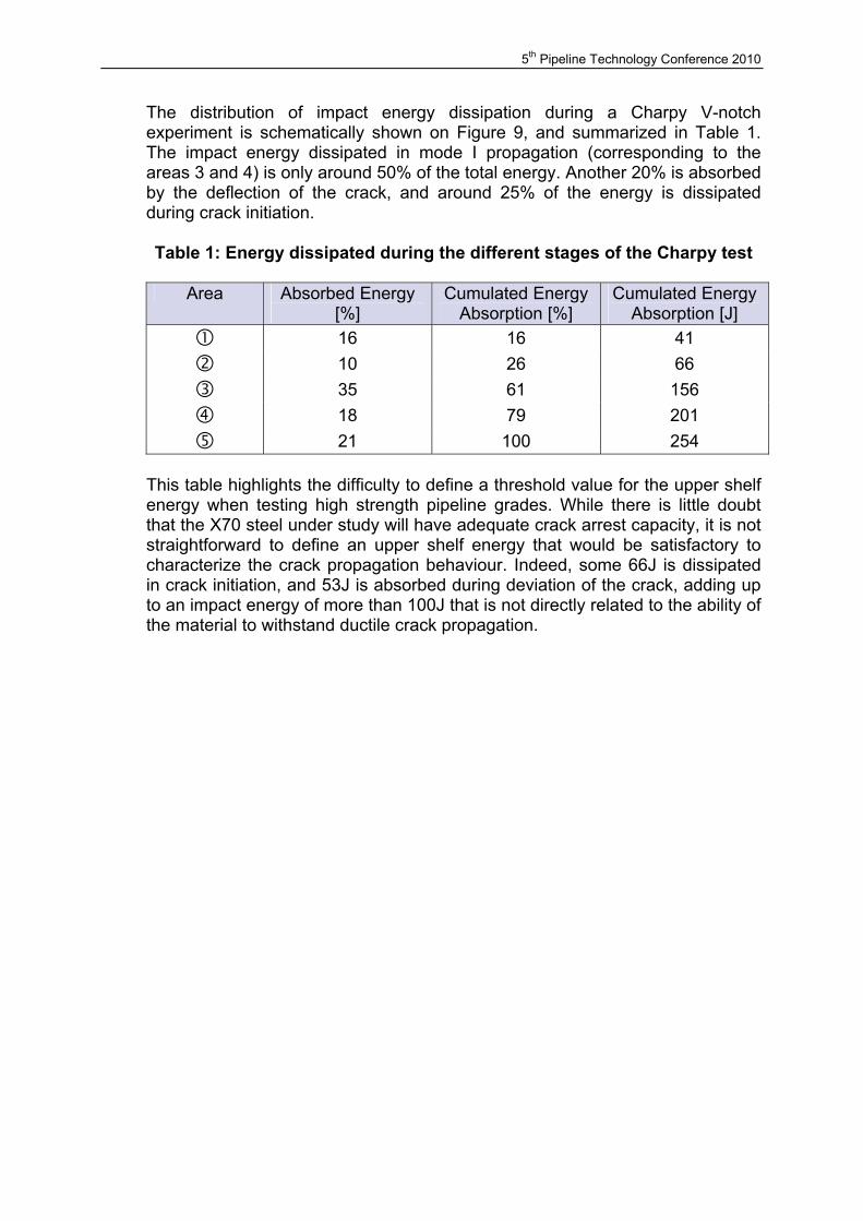
The distribution of impact energy dissipation during a Charpy V-notch experiment is schematically shown on Figure 9, and summarized in Table 1. The impact energy dissipated in mode I propagation (corresponding to the areas 3 and 4) is only around 50% of the total energy. Another 20% is absorbed by the deflection of the crack, and around 25% of the energy is dissipated during crack initiation. Table 1: Energy dissipated during the different stages of the Charpy test

Area Absorbed Energy

[%] Cumulated Energy

Absorption [%] Cumulated Energy

Absorption [J] 16 16 41 10 26 66 35 61 156 18 79 201 21 100 254

This table highlights the difficulty to define a threshold value for the upper shelf energy when testing high strength pipeline grades. While there is little doubt that the X70 steel under study will have adequate crack arrest capacity, it is not straightforward to define an upper shelf energy that would be satisfactory to characterize the crack propagation behaviour. Indeed, some 66J is dissipated in crack initiation, and 53J is absorbed during deviation of the crack, adding up to an impact energy of more than 100J that is not directly related to the ability of the material to withstand ductile crack propagation.


3. PREDICTING PIPE PROPERTIES The analysis in the previous section has shown that finite element methods can assist in obtaining a better understanding of the material behaviour, and support the development of enhanced toughness tests. Numerical techniques can provide an additional insight in the mechanical behaviour of linepipe steel during pipe manufacturing as well. In this section, the influence of the forming operations (bending, expansion) on the pipe properties is assessed. A numerical model is presented to predict the properties on pipe, based on the properties measured on the coil material. 3.1 Characterization of mechanical properties under reverse loading

In traditional design codes, the service pressure of a pipeline is proportional to the yield stress of the material. The linepipe standards [39-40] define the yield stress as the stress value reached for 0.5% of total deformation. Unfortunately, it is not possible to sample a straight specimen in hoop direction, and the pipe has to be flattened prior to tensile testing. This leads to a reverse deformation mode, and sometimes to a decrease of the yield stress on the pipe compared to the yield stress measured on the base material. This drop in mechanical properties is often referred to as the “Bauschinger effect” [41]. In the present investigation, different materials are tested in tensile-compression mode in order to provide data for a kinematic hardening model. Based on this experimental data set, a model is built to take into account several features of the material behaviour, like the presence of yield point elongation and the strain hardening.

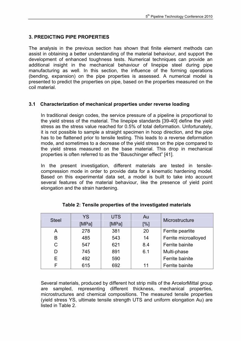
Table 2: Tensile properties of the investigated materials

YS UTS Au Steel

[MPa] [MPa] [%] Microstructure

A 278 381 20 Ferrite pearlite B 485 543 14 Ferrite microalloyed C 547 621 8.4 Ferrite bainite D 745 891 6.1 Multi-phase E 492 590 Ferrite bainite F 615 692 11 Ferrite bainite

Several materials, produced by different hot strip mills of the ArcelorMittal group are sampled, representing different thickness, mechanical properties, microstructures and chemical compositions. The measured tensile properties (yield stress YS, ultimate tensile strength UTS and uniform elongation Au) are listed in Table 2.


Alternate tensile/compression loading was performed in a range varying from 1% to 10% on a hydraulic testing system. At the end of each loading cycle, the radius

0

2

RyR

σ σ−= (16)

and the kinematic hardening

0

2

RyX

σ σ+= (17)

are measured, with σ0 the stress obtained at the end of the uniaxial loading, and R

yσ the yield stress after reverse loading, like schematically shown on Figure 10.

Figure 10: Definition of radius R and kinematic hardening X The evolution of the kinematic hardening and the radius of the yield surface were investigated in function of the pre-deformation and will be reported in [42]. The main observations are that

• The radius of the yield surface does not evolve significantly during the first percents of deformation, while the increase in kinematic hardening is much more pronounced.

• The kinematic hardening is more important for higher strength materials than for softer steel grades

• The kinematic hardening reaches an almost constant value for a pre-strain higher than 5%


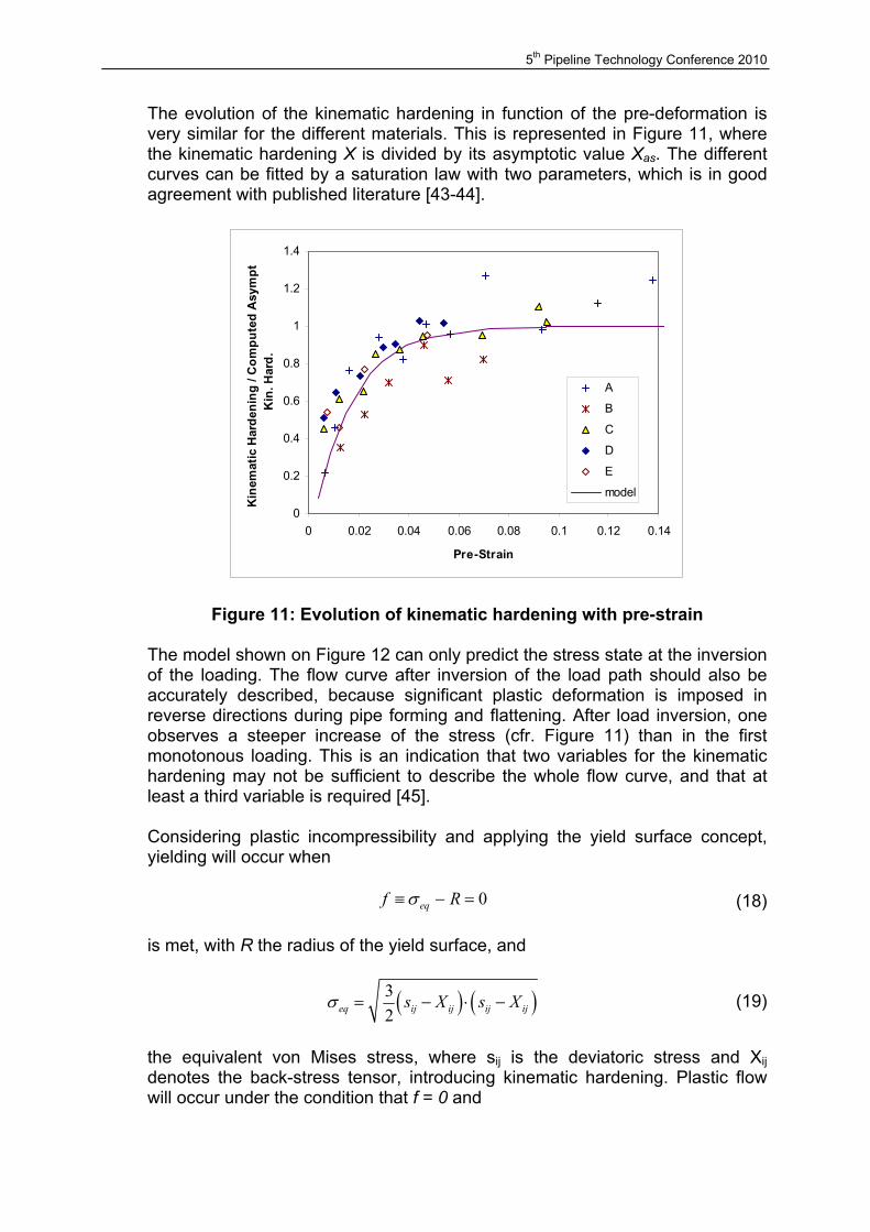
The evolution of the kinematic hardening in function of the pre-deformation is very similar for the different materials. This is represented in Figure 11, where the kinematic hardening X is divided by its asymptotic value Xas. The different curves can be fitted by a saturation law with two parameters, which is in good agreement with published literature [43-44].

0

0.2

0.4

0.6

0.8

1

1.2

1.4

0 0.02 0.04 0.06 0.08 0.1 0.12 0.14

Pre-Strain

Kin

emat

ic H

arde

ning

/ C

ompu

ted

Asy

mpt

K

in. H

ard.

A

B

C

D

E

model

Figure 11: Evolution of kinematic hardening with pre-strain The model shown on Figure 12 can only predict the stress state at the inversion of the loading. The flow curve after inversion of the load path should also be accurately described, because significant plastic deformation is imposed in reverse directions during pipe forming and flattening. After load inversion, one observes a steeper increase of the stress (cfr. Figure 11) than in the first monotonous loading. This is an indication that two variables for the kinematic hardening may not be sufficient to describe the whole flow curve, and that at least a third variable is required [45]. Considering plastic incompressibility and applying the yield surface concept, yielding will occur when

0eqf Rσ≡ − = (18) is met, with R the radius of the yield surface, and

( ) ( )32eq ij ij ij ijs X s Xσ = − ⋅ − (19)

the equivalent von Mises stress, where sij is the deviatoric stress and Xij denotes the back-stress tensor, introducing kinematic hardening. Plastic flow will occur under the condition that f = 0 and


/ : 0f σ σ∂ ∂ >& (20) The classical normality rule leads to the plastic strain rate tensor

ij

fs

ε λ ∂=

∂& (21)

where λ is the plastic multiplier. In the Lemaître-Chaboche model [43], the kinematic hardening tends to an asymptotic value Xsat at the same pace Ω1 during loading and after inversion:

( )1 sat plX N X X ε= Ω ⋅ ⋅ − ⋅& & (22)where

pl

pl

Nεε

=&

(23)

gives the direction of the deformation step. In our analysis, the amplitude of the saturation value Xsat is a function of the equivalent plastic deformation pl

eqε

( )21 exp plsat as eqX X ε = − −Ω (24)

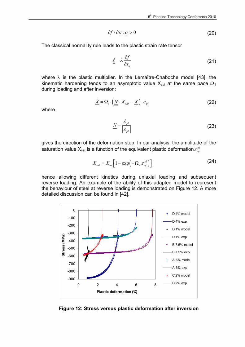
hence allowing different kinetics during uniaxial loading and subsequent reverse loading. An example of the ability of this adapted model to represent the behaviour of steel at reverse loading is demonstrated on Figure 12. A more detailed discussion can be found in [42].

-900

-800

-700

-600

-500

-400

-300

-200

-100

0

0 2 4 6 8

Plastic deformation (%)

Stre

ss (M

Pa)

D 4% model

D 4% exp

D 1% model

D 1% exp

B 7.5% model

B 7.5% exp

A 6% model

A 6% exp

C 2% model

C 2% exp

Figure 12: Stress versus plastic deformation after inversion


3.2 Characterization of mechanical properties under reverse loading

The previous paragraph has shown that numerical modelling is helpful to estimate the behaviour of pipeline steel in reverse loading, based on merely uniaxial tensile test data. On top of that, simulation techniques can be used to predict the change in properties when forming a steel plate or coil into a pipe. The forming operations that have to be addressed in such a study are

• Bending: transformation from a flat steel sheet to a bent pipe • Expansion: in some cases (e.g. the UOE pipe forming process [46]), the

pipe will be expanded. This is an equivalent step in case of forming with an expander, performing a hydrotest or ring expansion testing.

• Flattening: the pipe is flattened to allow sampling, which can be seen as a reverse bending operation.

• Tensile testing: after the different operations, uniaxial tension is applied to the flattened steel sample

These subsequent operations will lead to different deformations and stresses through the thickness of the sheet. As the length and width of the part are much larger than the thickness, the axial deformation is supposed to be homogeneous through the thickness. In addition, axial symmetry is assumed. As a result, the sheet/pipe can be discretized in the thickness only, dividing it in small slices for which the mechanical path is computed. During bending, the deformation at any position in the thickness can be expressed in function of the position of the slice relative to the neutral fibre [47]. Forming and flattening of the pipe are considered as similar bending operations in plane strain mode. Expansion, hydrotesting or ring expansion are similar load cases where an internal pressure is applied. We assume in these cases that the deformation in the z-direction is constant through the thickness. Finally, the tensile test is approximated by a strain increment in θ-direction, assuming no stress in the radial direction and a constant deformation in the z-direction. For spiral welded pipes, the transverse direction on pipe is different from the transverse direction on the skelp. Generally, hot rolled steel exhibits anisotropy of the mechanical properties, with the transverse direction being the direction with the highest mechanical properties. Crystal plasticity simulations have shown [48] that the difference between longitudinal and transverse directions could be computed based on the crystallographic texture of the material. From this knowledge about the mechanical properties in function of the direction and the angle of spiral forming, the softening of the material can be obtained. The prediction of pipe properties is extensively documented in [42]. Table 3 compares the measured and simulated yield stress for a ring expansion test before (B) and after (A) hydrotesting. A small difference between simulation and experimental data is observed, likely due to the difference in sampling for the base material (outer leap of the coil) compared to the position of the samples on pipe (83 m from the outer leap). However, the difference in yield stress before and after hydrotesting (4 MPa) is the same in the simulations and in the experimental results.


Table 3: Measured and calculated yield stress for ring expansion tests

Strip 90° top

90° bottom

180° top

180° bottom Av Calc

Sample [MPa] [MPa] [MPa] [MPa] [MPa] [MPa] [MPa]

α 510 499 501 510 510 529 B

β 510 499 507 509 513 508 529

α 516 508 513 512 512 533 β 511 - - 541 511 513 A γ 509 505 509 - - 507

533

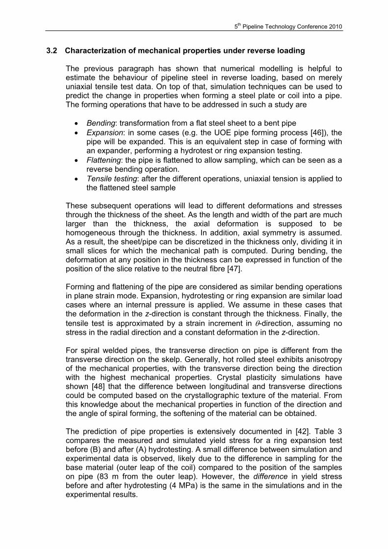
The simulated tensile curves corresponding to flattened samples after pipe forming are shown on Figure 13 and the corresponding numbers are reported in Table 4. One can observe that the model predicts a decrease of the yield stress after pipe forming and flattening compared to the base material, which is in line with the experimental data (solid lines). It also predicts that the tensile curves on pipe should be higher than the base material after a deformation of ~1.4.

Figure 13: Tensile curves before after of pipe forming and flattening In [42], the model predictions are compared with an industrial database containing different steel grades (from grade B to X80) and different ratios of wall thickness over diameter (t/D). The difference of yield stress between coil and pipe is predicted for the pipes in this database with good accuracy.


Table 4: Tensile test results before (B) and after (A) forming and flattening

Coil Experiment Calculation YS UTS YS UTS YS UTS

Coil Sample [MPa] [MPa] [MPa] [MPa] [MPa] [MPa]

B1 532 642 527 653 1

A1 569 647

523 633 521 563 B2 532 646 540 679

2 A2

567 673 522 639 537 679

B3 513 637 538 679 3

A3 580 672

509 639 533 679

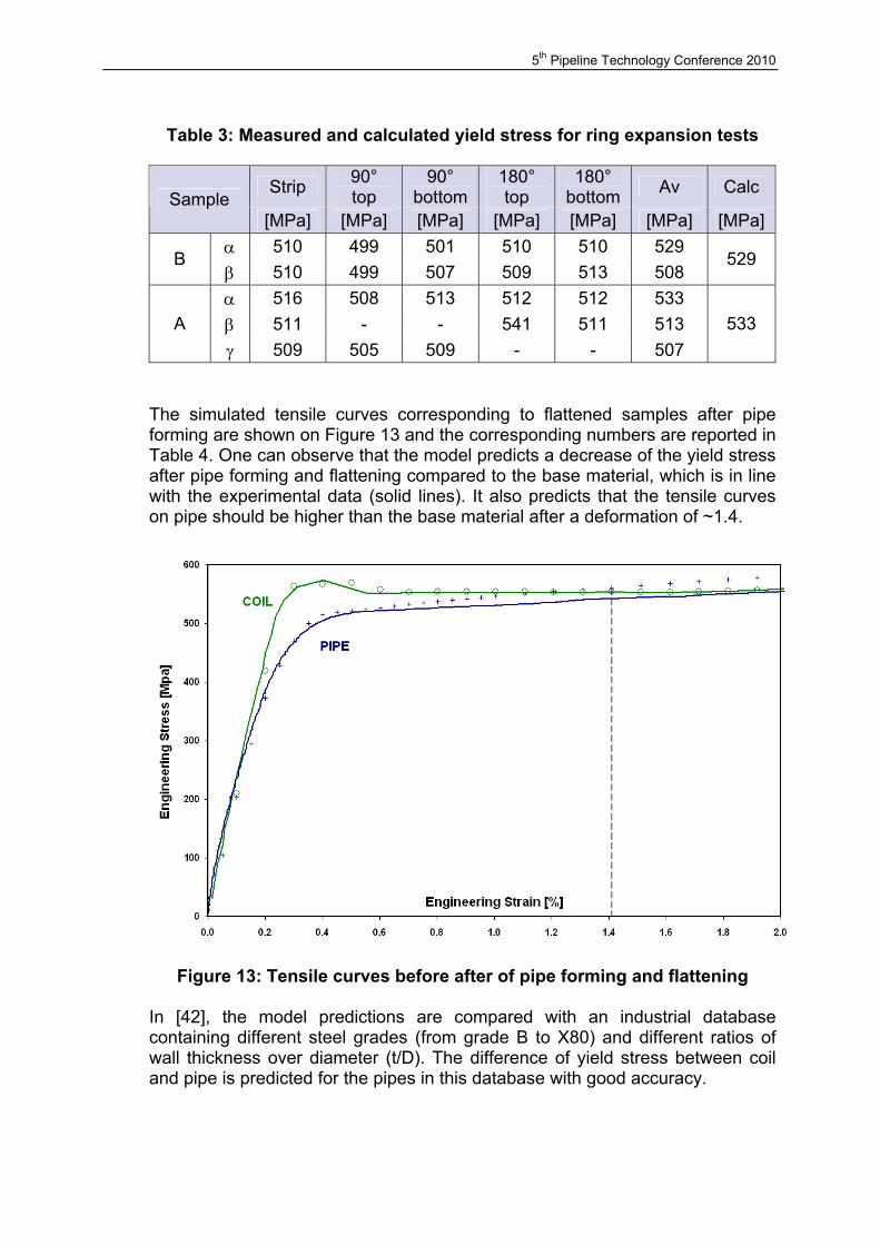
On Figure 14, the results of the model (yellow) are compared with experimental data (blue) for Electric Resistance Welded (ERW) pipes and High Frequency Induction (HFI) welded pipes. The accuracy of the model is ~20MPa, which is very good, as it captures not only the influence of the YS/UTS ratio (as would a statistical regression analysis), but the additional material information can give rise to a different prediction of the difference of yield stress for the same t/D ratio.

-50

-30

-10

10

30

50

70

90

110

130

150

0.012

0.014

0.014

0.015

0.016

0.016

0.016

0.017

0.018

0.020

0.021

0.021

0.0220.0

220.0

220.02

20.031

0.032

0.032

0.035

0.038

t/OD

delta

YS

(MPa

)

YS coil - YS pipe mill data YS coil - YS pipe model

Figure 14: Comparison between experimental database and predictions The previous sections have proven that numerical methods indeed can assist in modelling toughness of high strength pipeline steels, and predicting the change in mechanical properties between a coil and a manufactured pipe. In the next sections, the added value of Finite Element Analysis for pipeline engineering purposes is assessed by means of two case studies: the numerical design of composite crack arrestors for onshore pipelines, and mitigation measures for vortex induced vibrations in offshore pipeline spans.


4. CRACK ARRESTOR DESIGN FOR HIGH PRESSURE GAS PIPELINES One of the major challenges in the design of ultra high grade (X100) high pressure gas pipelines is the identification of a reliable crack propagation strategy. Like already shown in section 2, the newly developed high strength large diameter gas pipelines, when operated at severe conditions (rich gas, low temperatures, high pressure) may not be able to arrest a running ductile crack through intrinsic properties. Hence, the use of crack arrestors is required in the design of safe and reliable pipeline systems. Crack arrestors are usually classified as integral or non-integral, the first one consisting of pipes (or parts of pipes) acting as an integral part of the line, whereas the latter type is being made of mechanical devices mounted externally onto the pipeline. According to experimental results of full-scale tests, it is argued [49] that the most promising arrestors are

• Steel sleeve arrestors, in particular tight sleeves, which are placed around the main linepipe with a close fitting connection

• Composite crack arrestors, made of fibre reinforced plastics which

provide the pipe with an additional hoop constraint. The most commonly used composite crack arrestors are ClockSpring [50] and Composite Reinforced Linepipe (CRLP, [51]).

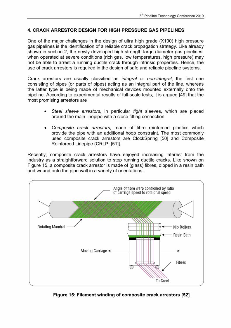
Recently, composite crack arrestors have enjoyed increasing interest from the industry as a straightforward solution to stop running ductile cracks. Like shown on Figure 15, a composite crack arrestor is made of (glass) fibres, dipped in a resin bath and wound onto the pipe wall in a variety of orientations.

Figure 15: Filament winding of composite crack arrestors [52]


In this paper, we want to emphasize the advantages numerical methods can bring to design composite crack arrestors. First, an analytical approach to estimate the properties of the composite material is presented. Then, orthotropic failure measures are proposed to predict the onset of material degradation. In the end, a numerical model is developed that can be used as a simulation tool for the safe design of composite crack arrestors. 4.1 Micromechanics of fibre reinforced plastics

The mechanical properties of fibre reinforced plastics depend on the fibre orientation. Therefore, the most commonly used composites are orthotropic materials, requiring 9 independent elastic constants to define the compliance matrix [53]. In the investigation, presented here, unidirectional (UD) glass fibre reinforced epoxy was identified as the most appropriate composite material to arrest a running crack. For such unidirectional reinforced laminates with adequate thickness, the constitutive law reduces to transverse isotropy, where only 5 constants are to be determined to build the stiffness matrix. The unknown elastic constants for each individual layer can be measured from static tensile tests and shear tests, or calculated by means of micromechanical mixture rules. The latter are used to calculate the elastic constants of composite materials, based on the properties of the (glass) fibre and the (epoxy) matrix. The properties of these constituents, and their volume fraction, are listed in Table 5. The stiffness matrix of the entire laminate is obtained by applying the Classical Laminate Theory [54], taking into account the fibre orientations of the different layers.

Table 5: Properties of glass fibre and epoxy matrix

E-glass fibre Epoxy matrix Stiffness Ef = 74 000 MPa Em = 3 500 MPa Poisson coefficient νf = 0.3 νm = 0.35 Density ρf = 2 555 kg/m³ ρm = 1 175 kg/m³ Tensile strength Xf = 3 450 MPa Xm = 60 MPa Volume fraction Vf = 0.6 Vm = 0.4

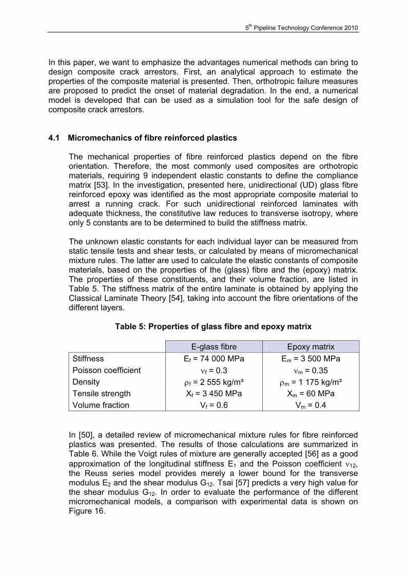
In [50], a detailed review of micromechanical mixture rules for fibre reinforced plastics was presented. The results of those calculations are summarized in Table 6. While the Voigt rules of mixture are generally accepted [56] as a good approximation of the longitudinal stiffness E1 and the Poisson coefficient ν12, the Reuss series model provides merely a lower bound for the transverse modulus E2 and the shear modulus G12. Tsai [57] predicts a very high value for the shear modulus G12. In order to evaluate the performance of the different micromechanical models, a comparison with experimental data is shown on Figure 16.


Figure 16: Comparison between the different micromechanical models The Voigt parallel model provides an excellent approximation for the longitudinal stiffness E1, and a good one for the Poisson coefficient ν12. The Reuss mixture rules provide a lower bound for E2 and G12, but do not correspond well with the experimental data. Only Greszczuck [58] and Hashin [59] give a reasonable estimation for the transverse modulus E2, and the shear stiffness G12 is predicted very well by both Hashin and Halpin-Tsai [55]. The other authors tend to overestimate the shear stiffness considerably. The Hashin model, which has been derived for unidirectional composites, shows the best agreement with the Resonalyser results.

4.2 Orthotropic failure criteria to predict material degradation

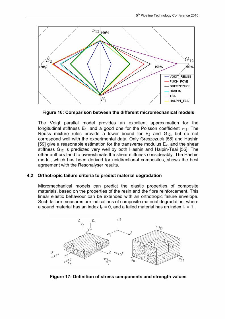
Micromechanical models can predict the elastic properties of composite materials, based on the properties of the resin and the fibre reinforcement. This linear elastic behaviour can be extended with an orthotropic failure envelope. Such failure measures are indications of composite material degradation, where a sound material has an index IF = 0, and a failed material has an index IF = 1.

Figure 17: Definition of stress components and strength values


When a composite layer with known strength values XT, XC, YT, YC, S, defined in Figure 17, is subjected to a combined in-plane loading σ11, σ22, τ12, the integrity of the material can be described by an appropriate failure criterion. A comprehensive overview of the most commonly used failure envelopes for unidirectional reinforced plastics is given in [55]. In this section, the Tsai-Hill criterion is introduced as a numerical tool to assist in the design of composite crack arrestors. Hill [61] proposed the yield criterion

( ) ( ) ( )( )

2 2 211 33 22 33 11 22

2 2 223 13 122 1

F G H

L M N

σ σ σ σ σ σ

τ τ τ

− + − + −

+ + + < (25)

as a generalization of the Von Mises (distortional energy) isotropic yield criterion for anisotropic materials. Tsai [62] adopted this criterion as a yield and failure measure for laminated composites:

2 2 211 11 22 22 12 1X X X Y Sσ σ σ σ τ − + + <

(26)

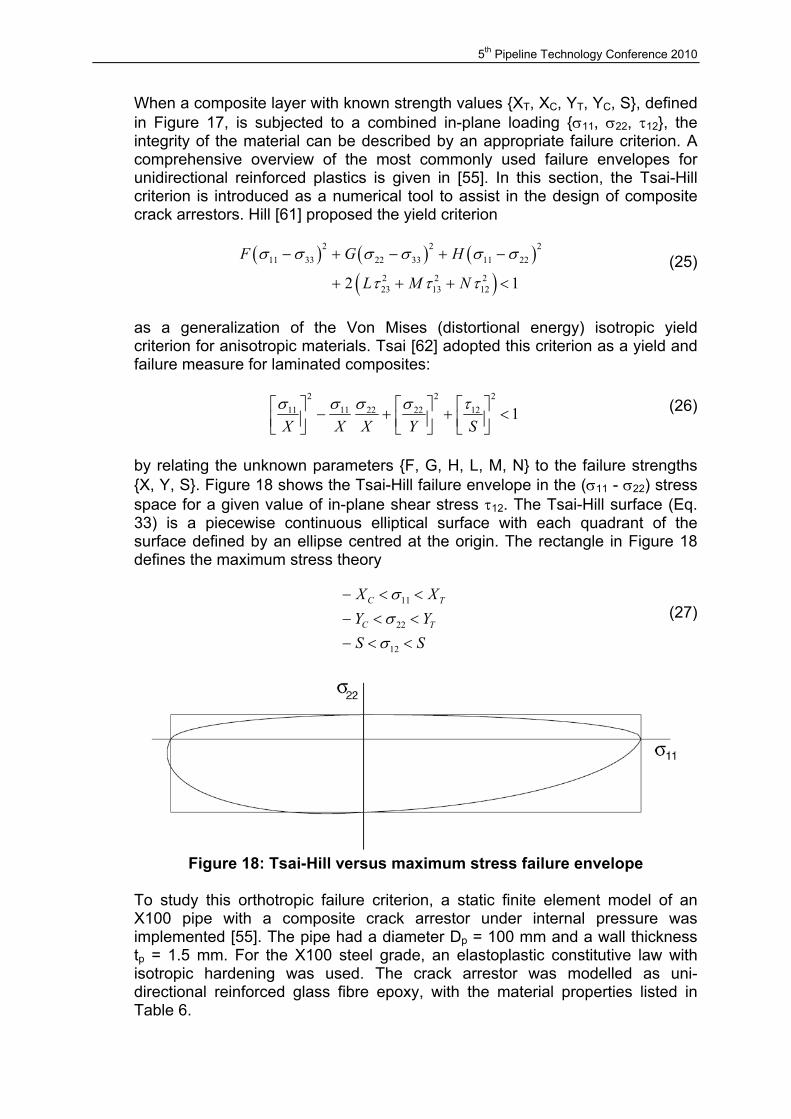
by relating the unknown parameters F, G, H, L, M, N to the failure strengths X, Y, S. Figure 18 shows the Tsai-Hill failure envelope in the (σ11 - σ22) stress space for a given value of in-plane shear stress τ12. The Tsai-Hill surface (Eq. 33) is a piecewise continuous elliptical surface with each quadrant of the surface defined by an ellipse centred at the origin. The rectangle in Figure 18 defines the maximum stress theory

11

22

12

C T

C T

X XY YS S

σσσ

− < <− < <− < <

(27)

Figure 18: Tsai-Hill versus maximum stress failure envelope

To study this orthotropic failure criterion, a static finite element model of an X100 pipe with a composite crack arrestor under internal pressure was implemented [55]. The pipe had a diameter Dp = 100 mm and a wall thickness tp = 1.5 mm. For the X100 steel grade, an elastoplastic constitutive law with isotropic hardening was used. The crack arrestor was modelled as uni-directional reinforced glass fibre epoxy, with the material properties listed in Table 6.


Table 6: Stiffness and strength values for UD glass fibre reinforced epoxy

E1 E2 = E3 ν12 = ν13 ν23 G12 = G13 G23 [MPa] [MPa] [-] [-] [MPa] [MPa] 44 200 11 400 0.356 0.343 4 420 5 027

XT YT XC YC R S [MPa] [MPa] [MPa] [MPa] [MPa] [MPa] 700 7.2 588 42 30 30

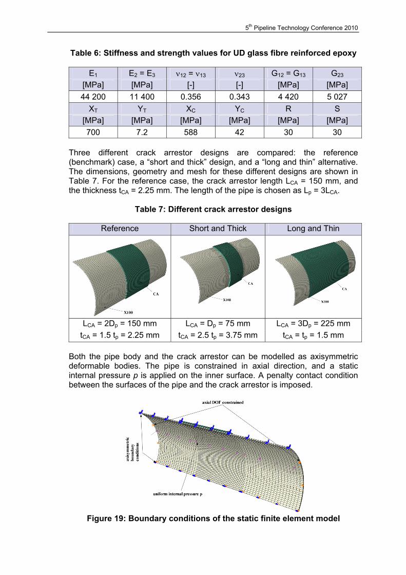
Three different crack arrestor designs are compared: the reference (benchmark) case, a “short and thick” design, and a “long and thin” alternative. The dimensions, geometry and mesh for these different designs are shown in Table 7. For the reference case, the crack arrestor length LCA = 150 mm, and the thickness tCA = 2.25 mm. The length of the pipe is chosen as Lp = 3LCA.

Table 7: Different crack arrestor designs

Reference Short and Thick Long and Thin

LCA = 2Dp = 150 mm LCA = Dp = 75 mm LCA = 3Dp = 225 mm tCA = 1.5 tp = 2.25 mm tCA = 2.5 tp = 3.75 mm tCA = tp = 1.5 mm

Both the pipe body and the crack arrestor can be modelled as axisymmetric deformable bodies. The pipe is constrained in axial direction, and a static internal pressure p is applied on the inner surface. A penalty contact condition between the surfaces of the pipe and the crack arrestor is imposed.

Figure 19: Boundary conditions of the static finite element model


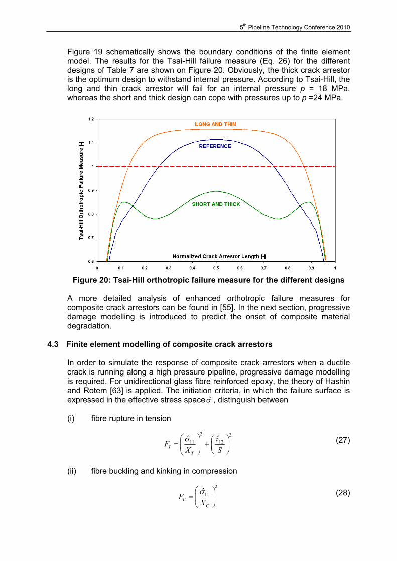
Figure 19 schematically shows the boundary conditions of the finite element model. The results for the Tsai-Hill failure measure (Eq. 26) for the different designs of Table 7 are shown on Figure 20. Obviously, the thick crack arrestor is the optimum design to withstand internal pressure. According to Tsai-Hill, the long and thin crack arrestor will fail for an internal pressure p = 18 MPa, whereas the short and thick design can cope with pressures up to p =24 MPa.

Figure 20: Tsai-Hill orthotropic failure measure for the different designs

A more detailed analysis of enhanced orthotropic failure measures for composite crack arrestors can be found in [55]. In the next section, progressive damage modelling is introduced to predict the onset of composite material degradation.

4.3 Finite element modelling of composite crack arrestors

In order to simulate the response of composite crack arrestors when a ductile crack is running along a high pressure pipeline, progressive damage modelling is required. For unidirectional glass fibre reinforced epoxy, the theory of Hashin and Rotem [63] is applied. The initiation criteria, in which the failure surface is expressed in the effective stress spaceσ , distinguish between (i) fibre rupture in tension

2 2

11 12ˆ ˆT

T

FX Sσ τ = +

(27)

(ii) fibre buckling and kinking in compression

2

11ˆC

C

FXσ

=

(28)


(iii) matrix cracking under transverse tension and shearing

2 2

22 12ˆ ˆT

T

MY Sσ τ = +

(29)

(iv) matrix crushing under transverse compression and shearing

2 2 2

22 22 12ˆ ˆ ˆ1

2 2C

CC

YMR R Y S

σ σ τ = + − +

(30)

The effective stress tensor σ is computed from ˆ Dσ σ= , where the damage operator

1 0 0

1

10 01

10 01

f

m

s

d

Dd

d

−

= −

−

(31)

can be constructed from the internal variables that characterize fibre damage

11

11

ˆ; 0ˆ; 0

Tf

C

Fd

Fσσ

≥= <

(32)

matrix damage

22

22

ˆ; 0ˆ; 0

Tm

C

Md

Mσσ

≥= <

(33)

and shear damage

( )( )( )( )1 1 1 1 1s T C T Cd F F M M= − − − − − (34)

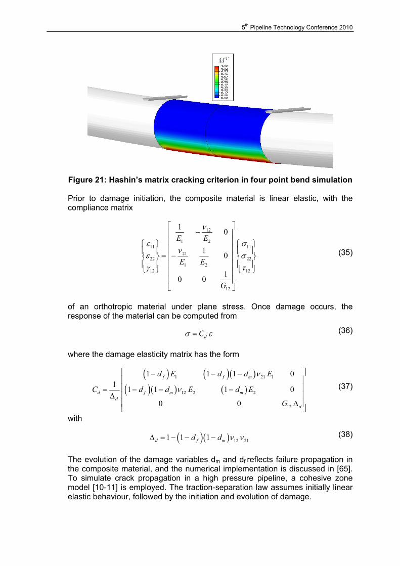
respectively. Guidelines on the calibration and application of the Hashin damage model for composite crack arrestors will be presented in [64]. The simulation of a four point bending test is shown on Figure 21, where the matrix cracking criterion (Eq. 29) predicts the onset of composite material failure.


Figure 21: Hashin’s matrix cracking criterion in four point bend simulation Prior to damage initiation, the composite material is linear elastic, with the compliance matrix

12

1 211 11

2122 22

1 212 12

12

1 0

1 0

10 0

E E

E E

G

ν

ε σνε σ

γ τ

−

= −

(35)

of an orthotropic material under plane stress. Once damage occurs, the response of the material can be computed from

dCσ ε= (36)

where the damage elasticity matrix has the form

( ) ( )( )( )( ) ( )

1 21 1

12 2 2

12

1 1 1 01 1 1 1 0

0 0

f f m

d f m md

d

d E d d E

C d d E d E

G

ν

ν

− − − = − − −

∆ ∆

(37)

with

( )( ) 12 211 1 1d f md d ν ν∆ = − − − (38)

The evolution of the damage variables dm and df reflects failure propagation in the composite material, and the numerical implementation is discussed in [65]. To simulate crack propagation in a high pressure pipeline, a cohesive zone model [10-11] is employed. The traction-separation law assumes initially linear elastic behaviour, followed by the initiation and evolution of damage.


Within the so-called process zone, material separation and fracture are controlled by a cohesive law which takes the general form t = f(δ), where t is the vector of surface tractions, and δ = [u] is the corresponding vector of displacement jumps between adjacent continuum elements. Damage initiation refers to the onset of material degradation, when the strains in the steel surface satisfy the quadratic nominal strain criterion

2 2 2

0 0 0 1n s t

n s t

ε ε εε ε ε

+ + =

(39)

where 0

nε , 0sε and 0

tε represent the peak values of the nominal strain when the deformation is either purely normal (n) to the interface, or only in the first (s) or the second (t) shear direction. The damage evolution law describes the rate at which the material stiffness is degraded once the initiation criterion (Eq. 39) is reached. A scalar damage variable D represents the overall damage in the pipe body and captures the combined effects of all the failure mechanisms. If damage evolution is accounted for, D monotonically evolves from 0 to 1 upon further loading after the initiation of damage. The stress components of the traction-separation model are affected by the damage according to

( )1t D t= − (40)

where t are the stress components predicted by the elastic traction-separation behaviour for the current strains without damage. To describe the evolution of damage under a combination of normal and shear deformation across the interface, it is useful to introduce an effective displacement [66] defined as

2 2 2

m n s tδ δ δ δ= + + (41)

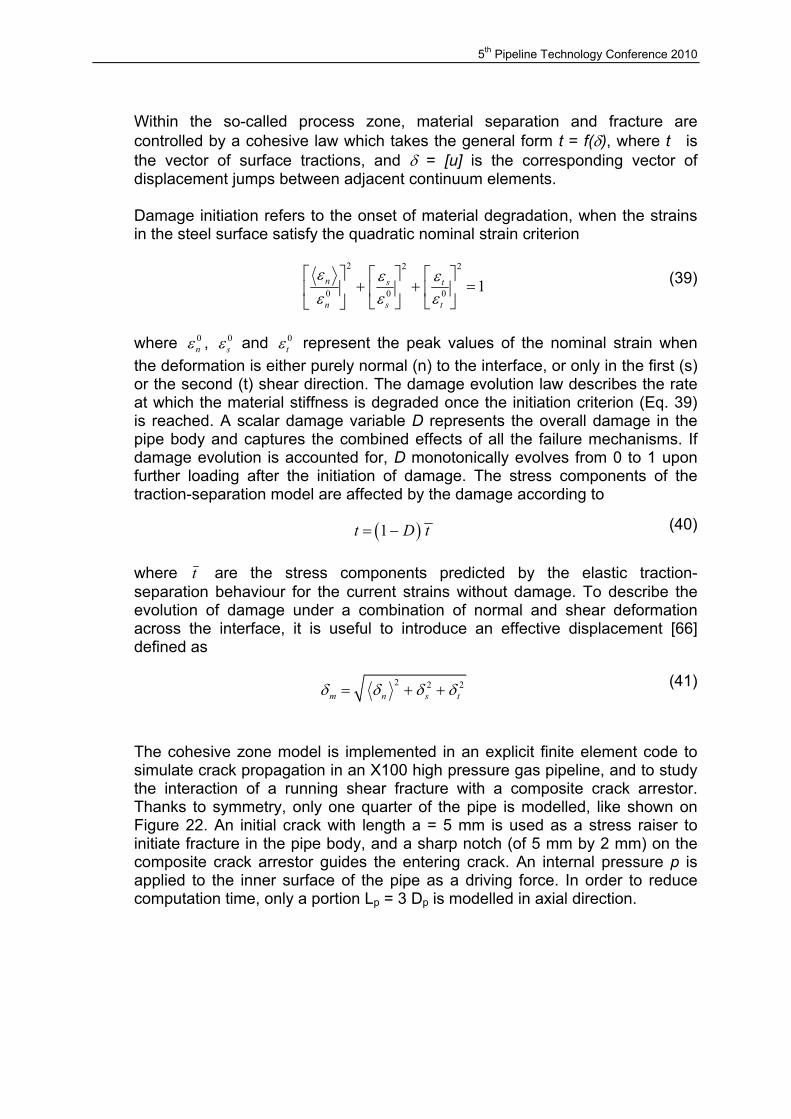
The cohesive zone model is implemented in an explicit finite element code to simulate crack propagation in an X100 high pressure gas pipeline, and to study the interaction of a running shear fracture with a composite crack arrestor. Thanks to symmetry, only one quarter of the pipe is modelled, like shown on Figure 22. An initial crack with length a = 5 mm is used as a stress raiser to initiate fracture in the pipe body, and a sharp notch (of 5 mm by 2 mm) on the composite crack arrestor guides the entering crack. An internal pressure p is applied to the inner surface of the pipe as a driving force. In order to reduce computation time, only a portion Lp = 3 Dp is modelled in axial direction.


Figure 22: Boundary conditions for the simulation of crack propagation

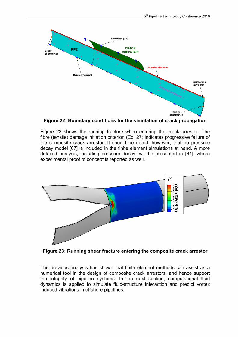
Figure 23 shows the running fracture when entering the crack arrestor. The fibre (tensile) damage initiation criterion (Eq. 27) indicates progressive failure of the composite crack arrestor. It should be noted, however, that no pressure decay model [67] is included in the finite element simulations at hand. A more detailed analysis, including pressure decay, will be presented in [64], where experimental proof of concept is reported as well.

Figure 23: Running shear fracture entering the composite crack arrestor

The previous analysis has shown that finite element methods can assist as a numerical tool in the design of composite crack arrestors, and hence support the integrity of pipeline systems. In the next section, computational fluid dynamics is applied to simulate fluid-structure interaction and predict vortex induced vibrations in offshore pipelines.


5. VORTEX INDUCED VIBRATIONS IN OFFSHORE PIPELINE SPANS Vortex induced vibration is a major cause of fatigue failure in submarine oil and gas pipelines and steel catenary risers [68]. Even moderate currents can induce vortex shedding, alternately at the top and bottom of the pipeline, at a rate determined by the flow velocity. Each time a vortex sheds, a force is generated in both the in-line and cross-flow direction, causing an oscillatory multi-mode vibration. This vortex induced vibration can give rise to fatigue damage of submarine pipeline spans, especially in the vicinity of the girth welds. In this section, Fluid-Structure Interaction (FSI) is applied to study the flow pattern around submarine pipeline spans, and predict the amplitude and frequency of the vortex induced vibrations. Computational fluid dynamics [69] provides a powerful means of comparing and evaluating the effectiveness of mitigation measures like helical strakes and fairings. 5.1 Analysis of offshore pipeline spans

A span can occur when an offshore pipeline bridges across a depression in the seabed, caused by a change in topology such as scouring or sand waves [70]. For a safe operation of offshore gas and oil pipelines during and after installation, these free spans should be limited to allowable lengths, which are determined during the design stage [71]. Indeed, when the free span is too long, the pipeline may suffer vortex induced vibration when the vortex shedding frequency is close to the natural frequency of the submarine pipeline span. For a pipe with diameter D and wall thickness t, the (lowest) natural frequency can be calculated as [72]

0 2e

C EIL m

ω = (42)

where me is the effective mass per unit length (including structural and added mass, and the fluid contained in the pipe), E is the Young’s modulus, C the end boundary coefficient and

3

2DI tπ =

(43)

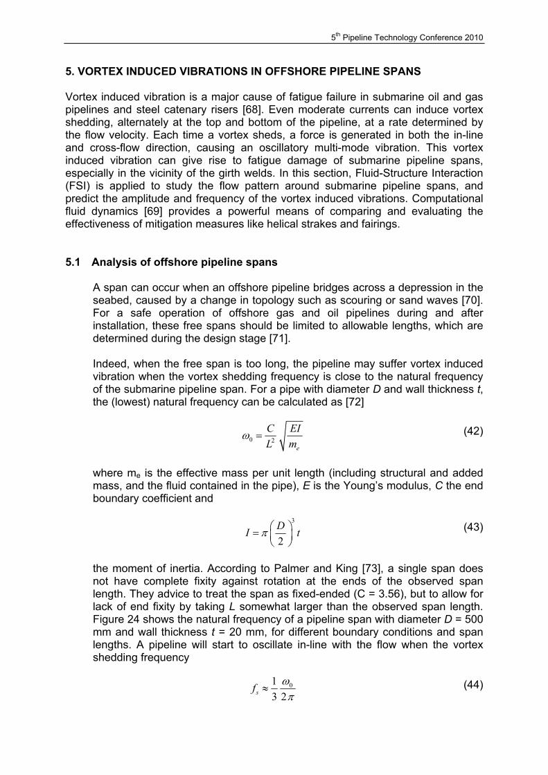
the moment of inertia. According to Palmer and King [73], a single span does not have complete fixity against rotation at the ends of the observed span length. They advice to treat the span as fixed-ended (C = 3.56), but to allow for lack of end fixity by taking L somewhat larger than the observed span length. Figure 24 shows the natural frequency of a pipeline span with diameter D = 500 mm and wall thickness t = 20 mm, for different boundary conditions and span lengths. A pipeline will start to oscillate in-line with the flow when the vortex shedding frequency

013 2sfωπ

≈ (44)


Figure 24: Influence of span length on natural frequency

Lock-in occurs when the vortex frequency fs is half of the natural frequency f0. As the flow velocity increases further, the cross-flow oscillation begins to occur and the vortex shedding frequency may approach the natural frequency of the pipeline span, which is detrimental to its fatigue lifetime. In the next section, numerical modelling of fluid-structure interaction is presented to predict vortex induced vibrations.

5.2 Computational Fluid Dynamics to Simulate Flow Patterns

Fluid flow around a cylinder is a well known and documented [74-76] problem in computational fluid dynamics, and often used as a benchmark [77] for CFD solvers. In this investigation, the benchmark is applied to study flow patterns behind submarine pipelines. The nature of the fluid flow is highly dependent on the Reynolds number

Re u Dυ

= (45)

expressing the ratio of inertia forces to viscous forces, where u is the fluid flow velocity, and the kinematic viscosity

µυρ

= (46)

is the ratio of the dynamic viscosity µ with the density ρ. A powerful Navier-Stokes solver is used to model unsteady, incompressible flow past a submarine pipeline. This CFD solver uses a generalized version of the Navier-Stokes equations


( )( ) ( )Tu u u u u p Ft

ρ µ ρ∂ − ∇⋅ ∇ + ∇ + ⋅∇ + ∇ = ∂

r rr r r r (47)

and accounts for incompressible flow by the equation of continuity

0u∇⋅ =

r (48)

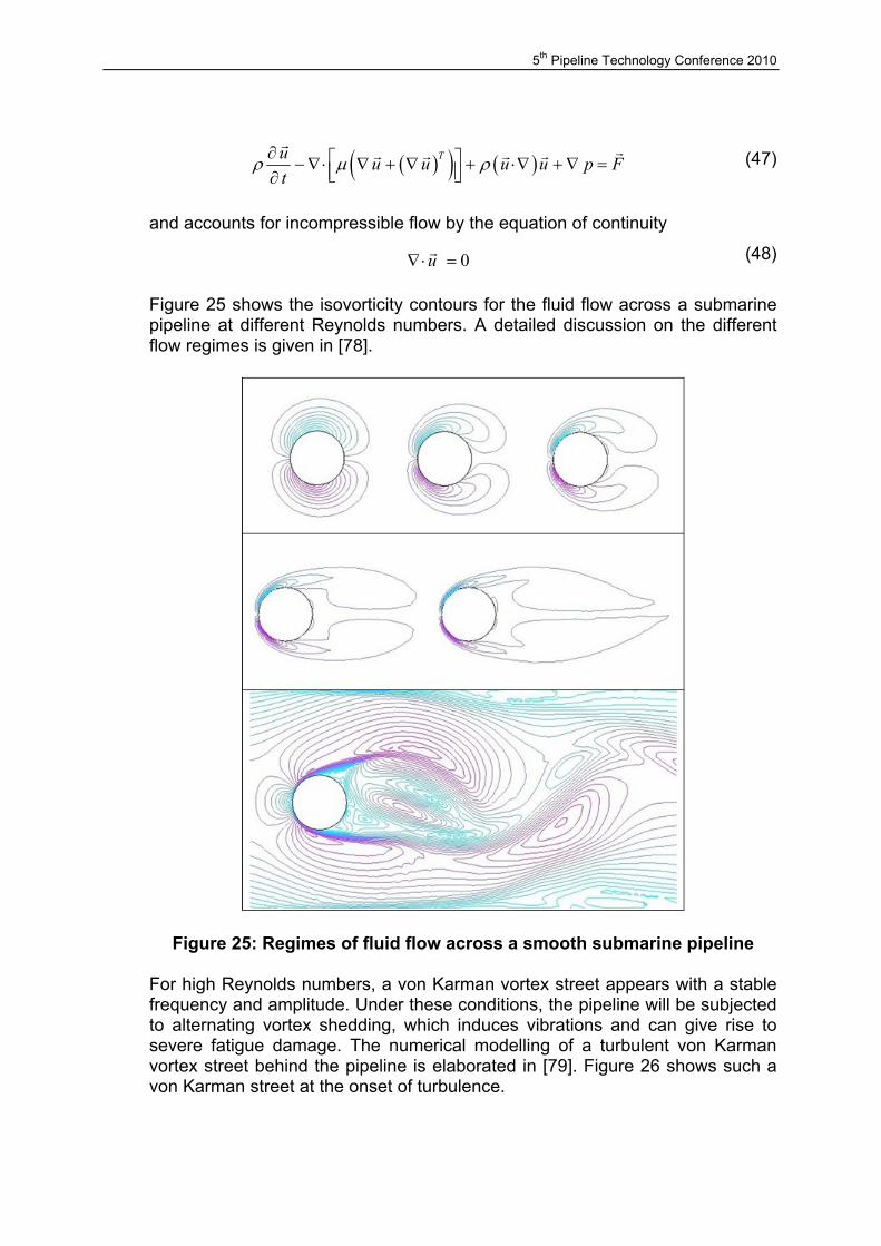
Figure 25 shows the isovorticity contours for the fluid flow across a submarine pipeline at different Reynolds numbers. A detailed discussion on the different flow regimes is given in [78].

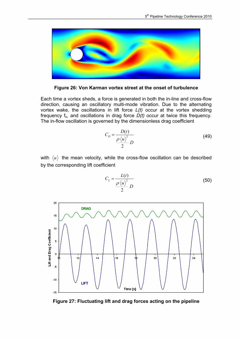
Figure 25: Regimes of fluid flow across a smooth submarine pipeline For high Reynolds numbers, a von Karman vortex street appears with a stable frequency and amplitude. Under these conditions, the pipeline will be subjected to alternating vortex shedding, which induces vibrations and can give rise to severe fatigue damage. The numerical modelling of a turbulent von Karman vortex street behind the pipeline is elaborated in [79]. Figure 26 shows such a von Karman street at the onset of turbulence.


Figure 26: Von Karman vortex street at the onset of turbulence Each time a vortex sheds, a force is generated in both the in-line and cross-flow direction, causing an oscillatory multi-mode vibration. Due to the alternating vortex wake, the oscillations in lift force L(t) occur at the vortex shedding frequency fs, and oscillations in drag force D(t) occur at twice this frequency. The in-flow oscillation is governed by the dimensionless drag coefficient

2( )

2

DD tCu

Dρ

= (49)

with u the mean velocity, while the cross-flow oscillation can be described by the corresponding lift coefficient

2( )

2

LL tCu

Dρ

= (50)

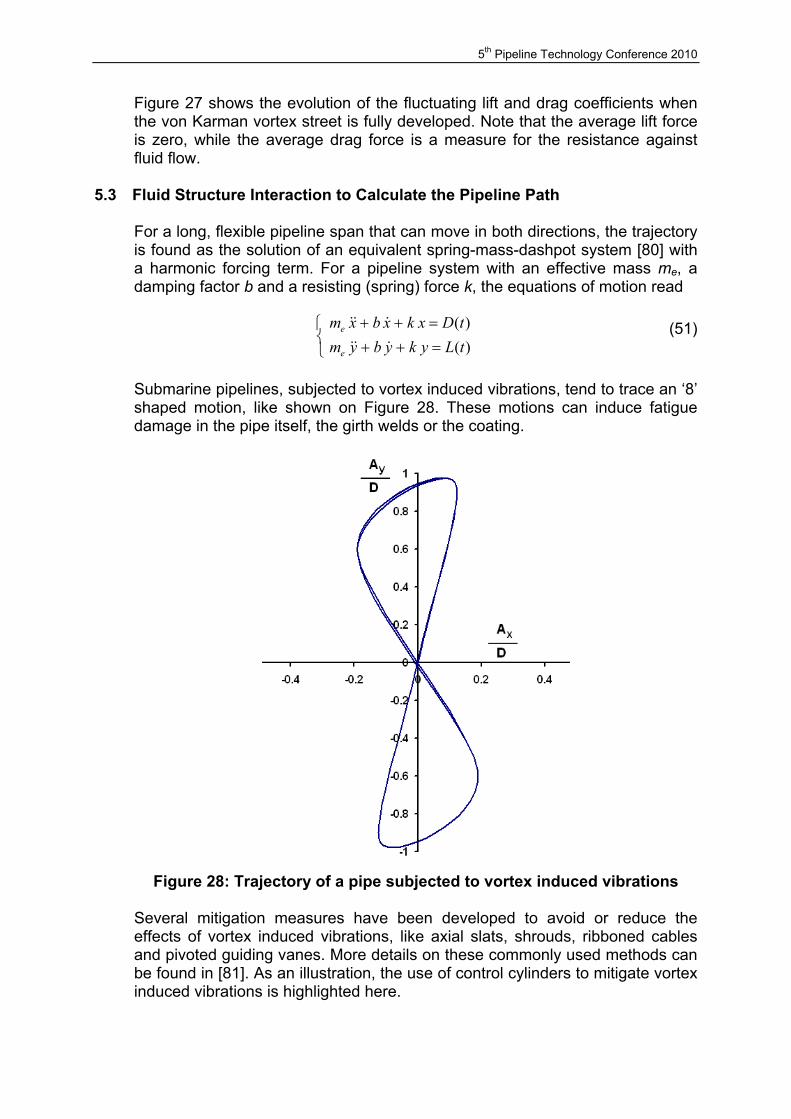
Figure 27: Fluctuating lift and drag forces acting on the pipeline


Figure 27 shows the evolution of the fluctuating lift and drag coefficients when the von Karman vortex street is fully developed. Note that the average lift force is zero, while the average drag force is a measure for the resistance against fluid flow.

5.3 Fluid Structure Interaction to Calculate the Pipeline Path

For a long, flexible pipeline span that can move in both directions, the trajectory is found as the solution of an equivalent spring-mass-dashpot system [80] with a harmonic forcing term. For a pipeline system with an effective mass me, a damping factor b and a resisting (spring) force k, the equations of motion read

( )( )

e

e

m x b x k x D tm y b y k y L t

+ + = + + =

&& &

&& & (51)

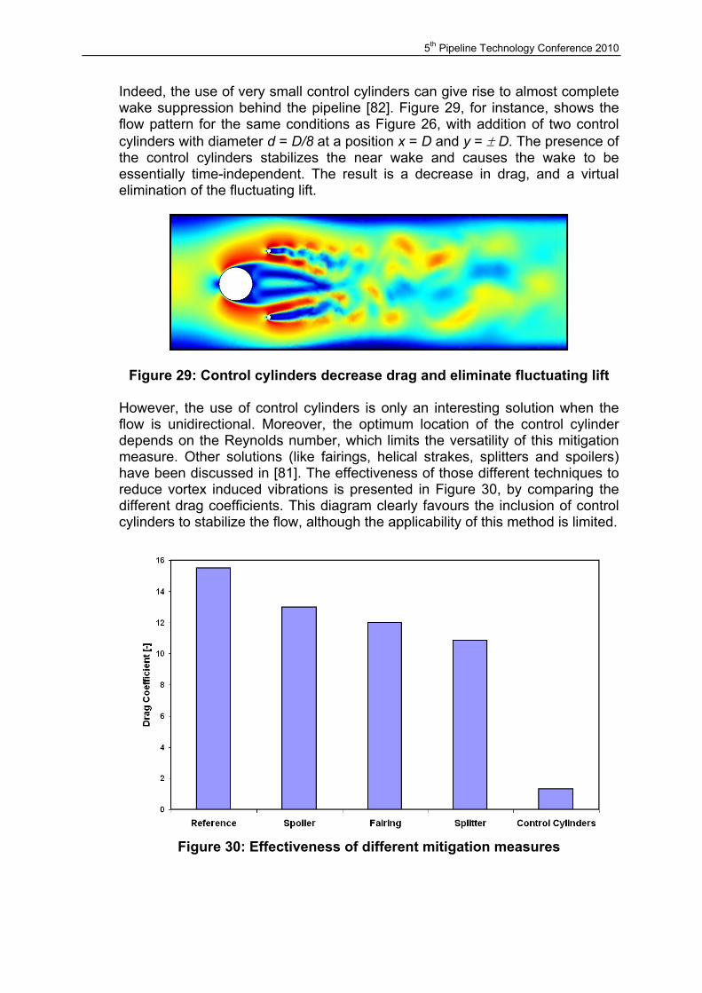
Submarine pipelines, subjected to vortex induced vibrations, tend to trace an ‘8’ shaped motion, like shown on Figure 28. These motions can induce fatigue damage in the pipe itself, the girth welds or the coating.

Figure 28: Trajectory of a pipe subjected to vortex induced vibrations

Several mitigation measures have been developed to avoid or reduce the effects of vortex induced vibrations, like axial slats, shrouds, ribboned cables and pivoted guiding vanes. More details on these commonly used methods can be found in [81]. As an illustration, the use of control cylinders to mitigate vortex induced vibrations is highlighted here.


Indeed, the use of very small control cylinders can give rise to almost complete wake suppression behind the pipeline [82]. Figure 29, for instance, shows the flow pattern for the same conditions as Figure 26, with addition of two control cylinders with diameter d = D/8 at a position x = D and y = ± D. The presence of the control cylinders stabilizes the near wake and causes the wake to be essentially time-independent. The result is a decrease in drag, and a virtual elimination of the fluctuating lift.

Figure 29: Control cylinders decrease drag and eliminate fluctuating lift However, the use of control cylinders is only an interesting solution when the flow is unidirectional. Moreover, the optimum location of the control cylinder depends on the Reynolds number, which limits the versatility of this mitigation measure. Other solutions (like fairings, helical strakes, splitters and spoilers) have been discussed in [81]. The effectiveness of those different techniques to reduce vortex induced vibrations is presented in Figure 30, by comparing the different drag coefficients. This diagram clearly favours the inclusion of control cylinders to stabilize the flow, although the applicability of this method is limited.

Figure 30: Effectiveness of different mitigation measures


6. CONCLUSION: AN EMERGING FIELD WITH PROMISING POTENTIAL In this paper, a simulation strategy to ensure pipeline integrity was proposed. The added value of numerical methods to assist in the safe design and operation of pipeline systems was discussed. The major conclusions read:

• Traditional fracture mechanics tests can be simulated using the finite element method and the GTN model. The simulations succeed in reproducing the load-deflection curve and calculating the J-integral for compact tension tests. Moreover, the finite element analysis enables a more profound interpretation of the Charpy test. Comparison between instrumented experiments and numerical simulations revealed that the linepipe steel dissipates enough energy in the initiation stage to fulfil the pipeline standards. Hence, finite element modelling can shed a brighter light on toughness properties of high strength pipeline steels. The models are currently being extended to account for existing flaws..

• To estimate the difference in yield stress between the coil and the pipe, a

numerical model was presented to calculate the deformation during bending and expansion. This model provides a more accurate description of the behaviour of the pipe body. The different loading paths can be combined to simulate pipe forming, flattening and subsequent tensile testing. The model includes a kinematic hardening law able to predict softening of the material in reverse loading, even in the case of yield point elongation. The model is capable of reproducing all features of the tensile curves after pipe forming, including the absence of yield point elongation and the decrease in yield stress. An extensive industrial database was used for experimental validation.

• A numerical tool to design composite crack arrestors for high pressure gas

pipelines was presented. Micromechanical modelling of unidirectional reinforced plastics revealed that the Hashin model is best fit to calculate the stiffness matrix, based on the properties of the fibre reinforcement and the resin. In addition, the Hashin progressive damage model is well-suited to predict the onset of composite material failure. In order to assess the ability of composite crack arrestors to stop a running fracture in a high pressure gas pipeline, a cohesive zone model was implemented. It was shown that finite element analysis can be an important asset in the design of composite crack arrestors, and hence contributes to the pipeline integrity.

• In the end, computational fluid dynamics was applied to study flow patterns

across submarine pipelines. For high Reynolds numbers, a turbulent von Karman vortex street appears in the pipeline wake, giving rise to multi-mode oscillations. Coupled calculations (fluid-structure interactions) can predict the pipeline trajectory. The vortex induced vibrations can give rise to severe fatigue damage of offshore pipelines. Multiphysics modelling allows evaluating and comparing different mitigation measures to suppress vortex shedding.

• Computational fracture mechanics is an emerging field in modern pipeline

engineering, and has a promising potential to reduce cost whilst ensuring integrity. Given the virtual nature of numerical methods, finite element analysis should always be validated and endorsed by experimental results.


REFERENCES [01] K-J Bathe, Finite Element Procedures in Engineering Analysis, Prentice-Hall

Inc., Englewood Cliffs, New jersey 07632, 735 pp. (1982) [02] O.C. Zienkiewicz, The Finite Element Method in Engineering Science, McGraw-

Hill Publishing Company Ltd, Berkshire England, 521 pp. (1971) [03] S.S. Rao, The Finite Element Method in Engineering, Fourth Edition, Elsevier

Science & Technology Books, 658 pp. (2004) [04] R.D. Cook, D.S. Malkus and M.E. Plesha, Concepts and Applications of Finite

Element Analysis, 3rd Edition, John Wiley and Sons (1989) [05] M.H. Aliabadi and D.P. Rooke, Numerical Fracture Mechanics, Solid Mechanics

and its Applications, Kluwer Academic Publishers, 275 pp. (1991) [06] M. Liebeherr, D. Ruiz Romera, B. Soenen, S. Ehlers and E. Hivert, Recent

Developments of High Strength Linepipe Steels on Coil, Proceedings of the 7th International Pipeline Conference, IPC2008-64295, Calgary, Canada (2008)

[07] M. Liebeherr, Ö.E. Güngör, R. Ottaviani, D. Lèbre, N. Llic, D. Quidort and S.

Ehlers, Production and Properties of X70 and X80 on Coil – Thickness in Excess of 20 mm, Proceedings of the 5th Pipeline Technology Conference, Ostend, Belgium (2009).

[08] Ö.E. Güngör, P. Thibaux, M. Liebeherr and D. Quidort, Evaluation and

Improvement of the Weld Properties in HFI Welded Pipes, Proceedings of the 5th Pipeline Technology Conference, Ostend, Belgium (2009)

[09] Ö.E. Güngör, P. Thibaux, M. Liebeherr and D. Quidort, Investigations into the

Microstructure – Toughness Relation in HFI Welded Pipes, Proceedings of the 8th International Pipeline Conference, IPC2010-31372, Calgary, Canada (2010)

[10] M. Liebeherr, N. Bernier, D. Lèbre, N. Llic and D. Quidort, Microstructure-

Property Relationship in 22m thick X80 Coil Skelp, Proceedings of the 8th International Pipeline Conference, IPC2010-31250, Calgary, Canada (2010)

[11] D. Ruiz Romera, M. Liebeherr, Ö. Güngör and D. Quidort, Development and

Weldability Evaluation of X100 on Coil, Proceedings of the 8th International Pipeline Conference, IPC2010-31372, Calgary, Canada (2010)

[12] G. Mannucci, M. Di Biagio, G. Demofonti, A. Fonzo, P. Salvini and A. Edwards,

Crack Arrestor Design by Finite Element Analysis for X100 Gas Transportation Pipelines, Proceedings of the 4th Pipeline Technology Conference, Ostend, Belgium (2004)


[13] G. Demofonti et. al., Fracture Propagation Resistance Evaluation of X100 TMCP Steel Pipes for High Pressure Gas Transportation Pipelines using Full-scale Burst Tests, Proceedings of the 4th Pipeline Technology Conference, Ostend, Belgium (2004)

[14] G. Mannucci and G. Demofonti, Control of Ductile Fracture Propagation in X80

Gas Linepipe, Proceedings of the 5th Pipeline Technology Conference, Ostend, Belgium (2009)

[15] D-J Shim, G. Wilkowski, D. Rudland, B. Rothwell and J. Merritt, Numerical

Simulation of Dynamic Ductile Fracture Propagation using Cohesive Zone Modelling, Proceedings of the 7th International Pipeline Conference, IPC2008-64049, Calgary, Canada (2008)

[16] I. Schiedel, M. Schöder, W. Borcks and W. Schönfeld, Crack Propagation

Analyses with CTOA and Cohesive Zone Model: Comparison and Experimental Validation, Engineering Fracture Mechanics, vol. 73, pp. 252-263 (2006)

[17] N. Bonora, A Non Linear Continuum Damage Mechanics Model for Ductile

Failure, Engineering Fracture Mechanics, vol. 58, pp. 11-28 (1997) [18] N. Bonora, Identification and Measurement of Ductile Damage Parameters,

Journal of Strain Analysis, vol. 34(6), pp. 463-478 (1999) [19] A.L. Gurson, Continuum Theory of Ductile Rupture by Void Nucleation and

Growth: Yield Criteria and Flow Rules for Porous Ductile Materials, Journal of Engineering Materials and Technology, vol. 99, pp. 2-15 (1977)

[20] V. Tvergaard, Influence of Voids on Shear Band Instabilities under Plane Strain

Conditions, International Journal of Fracture, vol. 17, pp. 389-407 (1981) [21] V. Tvergaard, On Localizations in Ductile Materials Containing Spherical Voids,

International Journal of Fracture, vol. 18, pp. 237-252 (1982) [22] V. Tvergaard and A. Needleman, An Analysis of Ductile Rupture in Notched

Bars, Journal of Mechanics and Physics of Solids, vol. 32, pp. 2-15 (1984) [23] V. Tvergaard and A. Needleman, Analysis of the Cup-Cone Fracture in a Round

Tensile Bar, Acta Metallica, vol. 32, pp. 157-169 (1984) [24] C. Chu and A. Needleman, Void Nucleation Effects in Biaxially Stretched

Sheets, Journal of Engineering Materials and Technology, pp. 249-256 (1980) [25] F. Van den Abeele and P. Thibaux, Computational Fracture Mechanics to Model

Toughness of Modern Pipeline Steels, Proceedings of the NAFEMS World Congress, Crete, Greece (2009)

[26] ASTM Standards, Standard Test Method for Plain Strain Fracture Toughness of

Metallic Materials, ASTM E399-90, American Society for Testing and Materials, Philadelphia (1997)


[27] M.F. Kanninen and C.H. Popelar, Advanced Fracture Mechanics, Oxford

University Press (1985) [28] D. Broek, Elementary Engineering Fracture Mechanics, Martinus Nijhoff

Publishers, (1986) [29] T.L. Anderson, Fracture Mechanics: Fundamentals and Applications, CRC

Press (2005) [30] M. Janssens, J. Zuidema and R.J. Wanhill, Fracture Mechanics, VSSD (2006) [31] P. Thibaux, S. Müller, B. Tanguy and F. Van den Abeele, Ductile Fracture

Characterization of an X70 Steel: Re-interpretation of Fracture Mechanics Tests Using the Finite Element Method, Proceedings of the 7th International Pipeline Conference, IPC2008-64291, Calgary, Canada (2008)

[32] ASTM Standards, Test Method for J-integral Characterization of Fracture

Toughness, ASTM E1820-08, American Society for Testing and Materials, Philadelphia (1996)

[33] M. Mohitpour, H. Golshan and A. Murray, Pipeline Design and Construction – A

Practical Approach, Third Edition, ASME press, 734 pp. (2007) [34] P. Thibaux and F. Van den Abeele, Determination of Crack Initiation and

Propagation Energy in Instrumented Charpy V-notch Impact Tests by Finite Element Simulations, Proceedings of the 5th Pipeline Technology Conference, Ostend, Belgium (2009)

[35] W.A. Maxey, J.F. Kierfner and R.J. Eiber, Brittle Fracture Arrest in Gas

Pipelines, Battelle Report to Line Pipe Research Supervisory Committee of the American Gas Association, NG-18 report n° 135 (1983)

[36] H. Huang and L. Xue, Prediction of Slant Ductile Failure Using Damage

Plasticity Theory, International Journal of Pressure Vessels and Piping, vol. 86, pp. 319-328 (2009)

[37] R. Eiber, T.A. Bubenic and W.A. Maxey, Fracture Control Technology for

Natural Gas Pipelines, American Gas Association, Catalogue n° 51691 (1993) [38] W.A. Maxey, Fracture Initiation, Propagation and Arrest, Proceedings of the 5th

Symposium on Line Pipe Research, Pipeline Research Council International, Catalogue n° L30174 (1974)

[39] American Petroleum Institute, API 5L Specification for Linepipe, 35th Edition,

101 pp. (1985) [40] International Standardisation Organisation, ISO 3183, Petroleum and Natural

Gas Industries – Steel Pipe for Pipeline Transportation Systems, 2nd Edition (2007)


[41] S.S. Yun and Y.W. Chang, Influence of Bauschinger Effect on Yield Stress after

Pipe Forming, Materials Science Forum vols. 475-479, pp. 4103-4108 (2005) [42] P. Thibaux and F. Van den Abeele, Influence of the Forming Operations on the

Yield Stress Measured on Pipe, Proceedings of the 8th International Pipeline Conference, IPC2010-31232, Calgary, Canada (2010)

[43] J. Lemaître and J.L. Chaboche, Mechanics of Solid Materials, Cambridge

University Press (1990) [44] P.J. Armstrong and C.O. Fredericks, A Mathematical Representation of the

Multiaxial Bauschinger Effect, Berkeley Nuclear Laboratories GEGB Report RS/B/N731

[45] H. Haddadi, S. Bouvier, M. Banu, C. Maier and C. Teodosiu, Towards an

Accurate Description of the Anisotropic Behaviour of Sheet Metals under Large Plastic Deformations: Modelling, Numerical Analysis and Identification, International Journal of Plasticity, vol. 22, pp. 2226-2271 (2006)

[46] M.D. Herynk, S. Kyriakides, A. Onoufriou and H.D. Yun, Effects of the

UOE/UOC Pipe Manufacturing Processes on Pipe Collapse Pressure, International Journal of Mechanical Sciences vol. 49, pp. 533-553 (2007)

[47] L. Delannay, R.E. Logé, J.W. Signorelli and Y. Chastel, Prediction of the Planar

Anisotropy of Springback after Bending of a Textured Zinc Sheet, Materials Processing and Design: Modelling, Simulation and Application, eds. S. Ghosh, J.C. Castro and J.K. Lee, pp. 1058-1063 (2004)

[48] P. Thibaux, D. Van Hoecke and G. De Vos, Influence of Forming and Flattening

on the Measured Tensile Properties of Linepipe, Proceedings of the 6th International Pipeline Conference, IPC2006-10116, Calgary, Canada (2006)

[49] B.N. Leis, E.B. Clark and R.J. Eiber, Crack Arrestor Review – Concepts, Design

and Testing and In-Service Use, Battelle Institute, report to BP Exploration and Production (2005)

[50] N.C. Fawley, Development of Composite Reinforced Materials for the Natural

Gas Industry, Annual Report of the Gas Research Institute, GRI-88/0264 (1988) [51] N.C. Fawley, Development of Fibre Glass Composite Systems for Natural Gas

Pipeline Service, NCF Industries Report to the Gas Research Institute, GRI-94/0072 (1994)

[52] F.C. Shen, A Filament Wound Structure Technology Overview, Materials

Chemistry and Physics, vol. 42, pp. 96-100 (1995) [53] R.M. Jones, Mechanics of Composite Materials, Scripta Book Company, 352

pp. (1975)


[54] K.S. Pister and S.B. Dong, Elastic Bending of Layered Plates, Journal of Engineering Mechanics, pp. 1-10 (1959)

[55] F. Van den Abeele and T. Skocovsky, Enhanced Failure Criteria for Composite

Crack Arrestors, Proceedings of the 5th Pipeline Technology Conference, Ostend, Belgium (2009)

[56] J.E. Ashton, J.C. Halpin and P.H. Petit, Primer on Composite Materials:

Analysis, Progress in Materials Science, Vol. III (1969) [57] S.W. Tsai, Structural Behaviour of Composite Materials, NASA CR-71 (1964) [58] L.B. Greszczuck, Damage in Composite Materials due to Low Velocity Impact,

Impact Dynamics, J.A. Zukas, J. Wiley & Sons (1982) [59] Z. Hashin, Failure Criteria for Unidirectional Fibre Composites, Journal of

Applied Mechanics, vol. 47, pp. 329-344 (1980) [60] J.C. Halpin and S.W. Tsai, Effects of Environmental Factors on Composite

Materials, AFML-TR 67-423 (1969) [61] R. Hill, Mathematical Theory of Plasticity, Oxford University Press, London

(1950) [62] S.W. Tsai, Strength Theories of Filamentary Structures, in ‘Fundamental

Aspects of Fibre Reinforced Plastic Composites’, eds. R.T. Schwartz and H.S. Schwartz, pp. 3-11, Wiley Interscience, New York (1968)

[63] Z. Hashin and A. Rotem, A Fatigue Criterion for Fibre Reinforced Materials,

Journal of Composite Materials, vol. 7, pp. 448-464 (1973) [64] F. Van den Abeele, L. Amlung, M. Di Biagio and S. Zimmermann, Design of

Composite Crack Arrestors for High Pressure Gas Pipelines, Proceedings of the 8th International Pipeline Conference, IPC2010-31191, Calgary, Canada (2010)

[65] I. Lapczyk and J.A. Hurtado, Progressive Damage Modelling in Fibre Reinforced

Materials, Composites Part A, vol. 38, pp. 2333-2341 (2007) [66] Hibbitt, Karlsson and Sorensen, Cohesive Elements Defined in Terms of

Traction-Separation, Abaqus Users’ Manual, pp. 26.5.6-1 – 26.5.6-10 (2008) [67] G. Berardo, P. Salvini, G. Mannucci and G. Demofonti, On Longitudinal

Propagation of a Ductile Fracture in a Buried Gas Pipeline: Numerical and Experimental Analysis, Proceedings of the 3rd International Pipeline Conference, Calgary, Canada (2000)

[68] R. King, A Review of Vortex Shedding Research and its Application, Ocean

Engineering, vol. 4, pp. 141-171 (1977)


[69] R.D. Gabbai and H. Benaroya, An Overview of Modelling and Experiments of Vortex Induced Vibration of Circular Cylinders, Journal of Sound and Vibration vol. 282, pp. 575-616 (2005)

[70] Danish Hydraulic Institute (DHI), Pipeline Free Span Design, Offshore Pipeline

Design Guide vol. 1, PR-170-9522 (1997) [71] H.S. Choi, Free Spanning Analysis of Offshore Pipelines, Ocean Engineering,

vol. 28, pp. 1325-1338 (2001) [72] R. Blevins, Formulas for Natural Frequency and Mode Shape, 503 pp., Krieger,

Florida (1979) [73] A. Palmer and R. King, Subsea Pipeline Engineering, 570 pp., Penwell

Publishing, Oklahoma (2004) [74] C. Norberg, Flow Around a Circular Cylinder: Aspects of Fluctuating Lift, Journal

of Fluids and Structures, vol. 15, pp. 459-469 (2001) [75] C. Norberg, Fluctuating Lift on a Circular Cylinder: Review and New

Measurements, Journal of Fluids and Structures, vol. 17, pp. 57-96 (2003) [76] D. Rocchi and A. Zasso, Vortex Shedding from a Circular Cylinder in a Smooth

and Wired Configuration: Comparison between 3D LES Simulation and Experimental Analysis, Journal of Wind Engineering and Industrial Aerodynamics, vol. 90, pp. 475-489 (2002)

[77] M. Schäfer and S. Turek, Benchmark Computations and Laminar Flow around a

Cylinder, Flow Simulation with High Performance Computers II, vol. 52, pp. 547-566 (1996)

[78] C. Farell and J. Blessmann, On Critical Flow Around Smooth Circular Cylinders,

Journal of Fluid Mechanics, vol. 136, pp. 375-391 (1983) [79] F. Van den Abeele, J. Vande Voorde and P. Goes, Numerical Modelling of

Vortex Induced Vibrations in Subsea Pipelines, Proceedings of the 4th COMSOL Users’ Conference, Hannover, Germany (2008)

[80] N. Jauvtis and C. Williamson, Vortex Induced Vibration of a Cylinder with Two

Degrees of Freedom, Journal of Fluids and Structures, vol. 17, pp. 1035-1042 (2003)

[81] F. Van den Abeele, P. Goes and J. Vande Voorde, Fluid-Structure Interaction to

Predict Fatigue Properties of Subsea Pipelines Subjected to Vortex Induced Vibrations, Proceedings of the 5th Pipeline Technology Conference, Ostend, Belgium (2009)

[82] C.H. Kuo, L.C. Chiou and C.C. Chen, Wake Flow Pattern Modified by Small

Control Cylinders at Low Reynolds Numbers, Journal of Fluids and Structures, vol. 23, pp. 938-956 (2007)

A Simulation Strategy to Ensure Pipeline Integrity · PDF fileA Simulation Strategy to Ensure...

Documents

Transcript of A Simulation Strategy to Ensure Pipeline Integrity · PDF fileA Simulation Strategy to Ensure...