Electronic copy available at: http://ssrn.com/abstract=2635537

A simulation-based methodology for evaluating hedge fund

investments

Marat Molyboga1

Efficient Capital Management

Christophe L’Ahelec2

Ontario Teachers’ Pension Plan

Keywords: large-scale simulation framework, hedge funds, optimal portfolios, risk parity, risk-

based allocations.

JEL Classification: G11, G17, C63

1Corresponding author: molyboga@efficient.com, Director of Research, 4355 Weaver Parkway, Warrenville, IL

60555 2Christophe_lahelec@ottp.com, Assistant Portfolio Manager, 5650 Yonge Street, Toronto, Ontario, M2M 4H5

Electronic copy available at: http://ssrn.com/abstract=2635537

Abstract

This paper introduces a large scale simulation framework for evaluating hedge funds’

investments subject to the realistic constraints of institutional investors. The method is

customizable to the preferences and constraints of individual investors, including investment

objectives, performance benchmarks, rebalancing period and the desired number of funds in a

portfolio and can incorporate a large number of portfolio construction and fund selection

approaches. As a way to illustrate the methodology, we impose the framework on a subset of

hedge funds in the managed futures space that contains 604 live and 1,323 defunct funds over

the period 1993-2014. We then measure the out-of-sample performance of three hypothetical

risk-parity portfolios and two hypothetical minimum risk portfolios and their marginal

contributions to a typical 60-40 portfolio of stocks and bonds. We find that an investment in

managed futures improves an investor’s performance regardless of portfolio construction

methodology and that equal risk approaches are superior to minimum risk portfolios across all

performance metrics considered in the study. Our paper is relevant for institutional investors in

that it provides a robust and flexible framework for evaluating hedge fund investments given

the specific preferences and constraints of individual investors.

Electronic copy available at: http://ssrn.com/abstract=2635537

The hedge fund industry represented about US $3 trillion in assets under management

(AUM) during the first quarter of 2015 according to the BarclayHedge Group. Therefore, hedge

funds represent a significant portion of the portfolios of institutional investors with direct

investments of US $2.5 trillion and an additional US $500 billion allocated through funds of

funds. While there is a rich literature on quantitative approaches to portfolio construction, it is

difficult to determine which method is optimal for an investor given his or her unique set of

investment constraints and preferences.

In this paper, we introduce a framework for the quantitative evaluation of portfolio

construction approaches subject to real life constraints. This methodology is implementable

because it explicitly accounts for the hedge fund reporting delay reported in Molyboga, Baek

and Bilson (2015), henceforth MBB, and applies an in-sample/out-of-sample framework that

incorporates common investment constraints when creating and rebalancing portfolios. The

framework imposes the standard requirements of institutional investors regarding track record

length and the amount of assets under management (AUM). It also limits the number of funds

in the portfolio and their turnover by assuming that the institutional investor selects a discrete

number of funds that stay in the portfolio until they no longer satisfy selection criteria3. The

methodology utilizes a simulation framework to account for a large number of feasible portfolio

constituents in each period. The framework is customizable to the preferences and constraints

of individual investors regarding rebalancing periods and the desired number of funds in a

portfolio and can incorporate a large number of portfolio construction and fund selection

approaches.

3 Fund selection criteria can incorporate performance-based ranking as in Molyboga, Baek and Bilson (2015).

We evaluate out-of-sample performance with several commonly used measures of

standalone performance and marginal portfolio contribution4. Standalone performance

measures include Annualized Return, Sharpe and Calmar ratios, maximum drawdown5 and the

t-statistic of alpha with respect to the Fung-Hsieh (2001) five-factor model. We measure

marginal portfolio contribution by evaluating the improvement in Sharpe and Calmar ratios6 by

replacing a modest 10% allocation of the original investor’s portfolio with a 10% allocation to a

simulated hedge fund portfolio. In this paper, we consider a standard 60-40 portfolio of stocks

and bonds as the original portfolio, but the framework is flexible to the choice of investor

benchmark.

Standard statistical techniques are inappropriate for the evaluation of out-of-sample

performance since simulation results are not independent, driven rather by the overlap in

portfolio constituents across simulations. We apply the bootstrapping methodology of Efron

(1979) and Efron and Gong (1983) to estimate the sampling properties of the test results and

draw statistical inferences about the relative performance of portfolio methodologies.

We impose the framework with 10,000 simulations on a dataset of 604 live and 1,323

defunct Commodity Trading Advisors over the period 1993-2014. Commodity Trading Advisors,

4 The framework is flexible and can incorporate customized performance measures selected by the investor. While the Fung-Hsieh (2001) five factor model is relevant for managed futures, the Fung-Hsieh eight factor model can be more appropriate for other types of hedge funds. MBB evaluate performance using second order stochastic dominance which is particularly relevant because investors are often unaware of their own utility functions as reported in Elton and Gruber (1987). Levy and Sarnat (1970) and Fischmar and Peters (2006) suggest using stochastic dominance as an alternative to mean-variance analysis. 5 See Chekhlov, Uryasev and Zabarankin (2005) for a formal definition of the maximum drawdown. It is typically defined as the largest peak-to-valley loss and represents a risk measure that is commonly used by practitioners. Calmar ratio is defined as the ratio of annualized excess return to the maximum drawdown. 6 Though in this paper marginal portfolio contribution is measured using Sharpe and Calmar ratios, in general it should be evaluated relative to the specific investment objectives of the investor. For example, a university endowment may target returns that exceed the university’s spending rate over a market cycle. The framework can incorporate investor-specific performance metrics of marginal portfolio contribution.

a subset of hedge funds that has grown exponentially over the past 35 years7, is known for its

historically strong performance during times of market crisis, notably the Financial Crisis of

2008, and, therefore, serves as a particularly interesting subset of hedge funds from a portfolio

diversification perspective. We evaluate several popular risk-based approaches that include

two minimum risk and three risk-parity methods. While the approaches we consider are

commonly used by both practitioners and academics, they are only a few of the portfolio

construction approaches that can be evaluated within the framework. The methodology can be

extended to a large number of quantitative portfolio construction approaches.

We find that an investment in CTAs improves performance regardless of the choice of

the portfolio construction approach. For the out-of-sample period between January 1999 and

December 2014, a 10% allocation to managed futures improves the Sharpe ratio of the original

60-40 portfolio of stocks and bonds from 0.376 to 0.399-0.416 on average, depending on the

portfolio construction methodology. Similarly, the Calmar ratio improves from 0.092 to 0.100-

0.108 on average. Blended portfolios have higher Sharpe ratios in at least 89% of simulations

and higher Calmar ratios in at least 89.5% of simulations. Minimum risk portfolios perform the

worst for all performance metrics. For example, their average Sharpe ratios are between 0.299

and 0.304, significantly lower than the 0.319 average Sharpe ratio of the random portfolios

from both an economic and statistical perspective. By contrast, equal risk methodologies

deliver superior average Sharpe ratios of 0.342 to 0.362. Our findings and methodology are

relevant for institutional investors who might consider investing or are currently invested in

7According to the BarclayHedge Group which monitors assets under management, Commodity Trading Advisors were managing $310 million in 1980, $10.5 billion in 1990 and $330 billion in the first quarter of 2015.

hedge funds and managed futures because the framework can be customized to the specific

preferences and constraints of investors to maximize benefits of hedge fund portfolios.

The remainder of the paper is organized as follows: Section I describes the data and

accounts for biases; Section II discusses the risk-based approaches and introduces the large

scale simulation framework; Section III presents empirical out-of-sample results; and Section IV

concludes.

I. Data

There are several commonly used CTA databases: BarclayHedge; CISDM (formerly the

MAR database); Lipper (formerly TASS); and Eurekahedge. Joenvaara, Kosowski and Tolonen

(2012) perform a comprehensive study of publicly available databases of hedge fund returns

and report that Barclay Hedge provides the highest quality data out of the databases

considered. Moreover, the BarclayHedge database is the largest publicly available database of

Commodity Trading Advisors with 1,013 active and 3,660 defunct funds over the period from

December 1993 to December 2014. Therefore, we use BarclayHedge for this study as it is the

most comprehensive and highest quality publicly available database of CTA returns.

We perform a number of filtering steps to ensure data quality and limit the scope of the

study to the funds that would be appropriate for institutional investors who are interested in

making direct investments. We explicitly account for the survivorship, backfill, incubation and

liquidation biases that are common within CTA and hedge fund databases8. We include the

graveyard database that contains defunct funds to account for the survivorship bias. The

8 For details, see Appendix A: Data cleaning.

backfill and incubation biases arise due to the voluntary nature of self-reporting9. We use a

combination of two approaches to mitigate these biases. The first methodology, suggested by

Fama and French (2010), limits the tests to those funds that managed at least US $10 million in

AUM normalized to December 2014 values. Once a fund reaches the AUM minimum, it is

included in all subsequent tests to avoid creating selection bias. Unfortunately, many CTAs,

including very successful and established ones, originally reported only net returns for an

extended period of time prior to their initial inclusion of AUM data. Using Fama and French

(2010) methodology exclusively would completely eliminate large portions of valuable data for

such funds. To include this data, we apply the technique suggested by Kosowski, Naik and Teo

(2007), which eliminates only the first 24 months of data for such funds. We use the liquidation

bias estimate of 1% as suggested in Ackermann, McEnally and Ravenscraft (1999). After

accounting for the biases, our dataset includes 604 live and 1,323 defunct funds for the period

between December 1995 and December 2014.

We use the Fung-Hsieh five factor model of primitive trend following systems,

introduced in Fung and Hsieh (2001), as benchmarks in measuring the performance of CTA

portfolios. The factors include PTFSBD (bonds), PTFSFX (foreign exchange), PTFSCOM

(commodities), PTFSIR (interest rates) and PTFSSTK (stocks) while the 3-month Treasury bill

(secondary market rate) series with ID TB3MS from the Board of Governors of the Federal

Reserve System serves as a proxy for the risk-free rate. Table I reports summary statistics and

9 Typically funds go through an incubation period during which they build a track record using proprietary capital. Fund managers choose to start reporting to a CTA database to raise capital from outside investors only if the track record is attractive and they are allowed to “backfill” the returns generated prior to their inclusion in the database. Since funds with poor performance are unlikely to report returns to the database, incubation/backfill bias results.

tests of normality, heteroscedasticity and serial correlations in CTA returns by strategy and

current status.

<Put Table I here>

Anson (2011) suggests that the 60-40 portfolio of stocks and bonds represents a typical

starting point for a US institutional investor. In this paper, this blend is constructed using the

S&P 500 Total Return index and the JPM Global Government Bond Index. Table II reports the

annualized excess return, standard deviation, maximum drawdown, Sharpe ratio and Calmar

ratio of the 60-40 portfolio for 1999-2014. Over this time period, the portfolio delivered a

Sharpe ratio of 0.376 and a Calmar ratio of 0.092.

<Table II>

Figure 1 shows the performance of the portfolio from January 1999 to December 2014.

<Put Figure 1 here>

Although the 60-40 portfolio of stocks and bonds has been used extensively in the literature as

a benchmark portfolio, the framework is flexible and can incorporate any investor-specific

portfolio as a benchmark.

II. Methodology

In this section, we define the risk-based approaches considered in this study. Then we

introduce a large-scale simulation framework with real-life constraints used to generate out-of-

sample portfolio returns. Finally, we describe the performance metrics used to compare out-

of-sample results.

A. Review of risk-based approaches

In this paper, we evaluate two minimum risk and three equal-risk (or risk-parity) approaches10.

While the approaches we consider are commonly used by practitioners and academics, they are

used merely as examples of portfolio construction approaches that can be evaluated within the

framework. The methodology can be extended to a large number of quantitative portfolio

construction approaches. Minimum risk portfolios include the minimum variance (MV)

approach with non-negative constraints documented in Jagannathan and Ma (2003) and a

minimum semi-standard deviation (MDEV) approach that is similar to the minimum variance

approach but only considers negative returns. Equal-risk, or risk-parity, approaches include an

equal notional (EN) approach, which is a naïve diversification 1/N method praised in DeMiquel,

Garlappi and Uppal (2009) and criticized in Kritzman, Page and Turkington (2010), an equal

volatility-adjusted (EVA) approach highlighted in Hallerbach (2012) and the classical risk parity

(RP) approach extensively discussed in Maillard, Roncalli and Teiletche (2010), Clarke, Silva and

Thorley (2013) and Qian (2013). We apply a random portfolio selection approach (Random)

that serves as a benchmark in evaluating the risk parity approaches. The approaches are

evaluated using a large-scale simulation framework with real life constraints.

B. Large scale simulation framework

In this paper, we utilize a modification of the large-scale simulation framework with real life

constraints introduced in MBB. MBB apply the framework to evaluate persistence in hedge

fund managers’ performance and compare equally-weighted portfolios of funds that rank in the

10 See Appendix B for technical definitions of the risk-based approaches.

top quintile based on the t-statistic of alpha with respect to a CTA benchmark (restrictive fund

selection) against those of all available funds (random fund selection). By contrast, this paper

does not impose any ranking but rather focuses on the impact of choice of portfolio

construction methodology on performance. The out-of-sample period is between January 1999

and December 2014, the longest out-of-sample backtesting period in CTA empirical research.

The framework uses 10,000 simulations and a lag of one month to account for the delay in the

performance reporting of CTAs11. Below we describe a single run of the simulation framework

and then show how simulation results are evaluated.

i) A single run of the simulation framework

The in-sample/out-of-sample framework mimics the actions of an institutional investor who

makes allocation decisions at the end of each month. The first decision is made in December

1998. Due to the delay in CTA reporting, the investor has return information only through

November 1998; thus, the investor considers all funds that have a complete set of monthly

returns between December 1995 and November 1998. First, the investor eliminates all funds in

the bottom quintile of AUM among the funds considered. This relative AUM threshold is more

appropriate than the fixed AUM approach commonly used in the literature (for example,

Kosowski, Naik and Teo (2007) use a fixed AUM level of US $20 million) because the average

level of AUM has increased substantially over the last 20 years. Then the investor randomly

chooses 5 funds from the remaining pool of CTAs and allocates to them using the five risk-

based approaches and a random portfolio allocation. Monthly returns are recorded for each

11 See MBB for a detailed description of the hedge fund reporting delay.

portfolio construction approach for January 1999 using the liquidation bias adjustment for

funds that liquidate during the month. At the end of January 1999, the pool of CTAs is updated

and defunct constituents of the original portfolio are randomly replaced with funds from the

new pool. Each portfolio is then rebalanced again using the original portfolio construction

methodologies12. The process is repeated until the end of the out-of-sample period of

December 2014. A single simulation results in six out-of-sample return streams between

January 1999 and December 2014 – one for each of the portfolio construction approaches.

ii) Performance evaluation of out-of-sample results.

Out-of-sample performance is evaluated using both standalone performance metrics and

measures that consider portfolio contribution benefits. Standalone performance metrics

include annualized return, maximum drawdown, Sharpe ratio, Calmar ratio13, Fung-Hsieh alpha

and t-statistic of alpha. Performance contribution is measured as the resultant difference in

Sharpe ratio and Calmar ratio from replacing 10% of the original portfolio of stocks and bonds

with portfolios of CTA funds constructed within the simulation framework. Since each

performance measure is represented by a distribution that contains 10,000 values, distributions

are compared using means and medians for all measures and the percentage of positive values

for Fung-Hsieh alpha and the percentage of positive marginal Sharpe and Calmar ratios in the

performance contribution measures. Since simulations are not independent, we apply a

bootstrapping procedure to draw statistical inference.

12 The framework is flexible – the number of funds in a portfolio, rebalancing frequency, AUM threshold levels and other parameters can be customized to reflect each investor’s preferences and constraints. 13 Calmar ratio is defined as the ratio of the annualized excess return to the maximum historical drawdown.

iii) Boostrapping procedure

The bootstrapping procedure follows each steps of the simulation framework but limits the set

of portfolio construction approaches to the Random portfolio methodology to which we choose

to compare all other approaches14. Each simulation set consists of 10,000 simulations. The

bootstrapping procedure includes 400 sets of simulations, a sufficient number to estimate p-

values with high precision. A comparison of the performance metrics of the original simulation

to the bootstrapped sets of simulations gives the p-values reported in the empirical results

section.

III. Empirical out-of-sample results.

In this section, we present information about the dataset used in the simulation and out-of-

sample results for the period between January 1999 and December 2014 generated by the

large-scale simulation framework.

Table III reports the average AUM threshold level for each year and the average number of

funds meeting that threshold. The AUM threshold represents the 20th percentile of AUM

among all active fund managers with a track record of at least 36 months.

<Table III>

There is a significant variation in the values of the AUM threshold over time which primarily

reflects changes in assets under management driven by industry growth and recent

performance. The 2010 threshold value of US $13.97 million is almost three times as high as

14 The framework is flexible in comparing any two approaches to each other but requires performing additional bootstrapping simulations based on an investor’s particular areas of interest.

the US $5 million threshold value in 2001. The number of funds has nearly doubled over this

time period representing substantial growth in the industry.

A. Analysis of out-of-sample performance of CTA portfolios as standalone investments

We analyze distributions of out-of-sample returns over the complete data period using means

and medians of several performance metrics. Since simulations are not independent, we use a

bootstrapping methodology to draw statistical inferences about the relative performance of

portfolio construction approaches.

i) Distributions of out-of-sample performance

Table IV reports means and medians for the distributions of returns, volatilities, Sharpe and

Calmar ratios and maximum drawdowns for each portfolio construction approach. The p-

values are estimated using the bootstrap methodology. The superscript star indicates that the

performance measure of a given portfolio approach exceeds that of the RANDOM portfolio at

99% confidence level. The subscript star shows that the performance measure of a given

portfolio approach is lower than that of the RANDOM portfolio at 99% confidence level.

<Table IV>

The minimum risk approaches tend to have the lowest volatilities of the portfolio

methodologies considered in the study. MV and MDEV have mean volatilities of around 6.8%

whereas EVA and RP have volatilities of around 8.21% and 8.66%, respectively, followed by EN

and RANDOM with volatilities that exceed 11%. However, the lower levels of volatility are not

necessarily associated with lower drawdowns. For example, EVA has a maximum drawdown of

19.12%, slightly lower than the 19.9% maximum drawdown values of the minimum risk

portfolios. Moreover, the minimum volatility approaches deliver low returns and risk-adjusted

returns that are inferior to those of the other approaches. This finding is consistent with

DeMiquel, Garlappi and Uppal (2009) which documents the superior out-of-sample

performance of the naïve 1/N (EN) approach relative to that of several extensions of mean-

variance optimization including the minimum variance (MV) approach. Jensen’s inequality

suggests the EN approach should dominate the RANDOM methodology in terms of Sharpe ratio

due to the concavity of the Sharpe ratio15. The three equal-risk approaches have risk-adjusted

performance which is superior to that of the RANDOM approach. In contrast, minimum risk

approaches yield inferior results on average. Median values reported in Panel B show similar

results.

While Table IV presents mean and median values of several performance metrics, a

complete evaluation of the portfolio construction methodologies should also consider

distributions of out-of-sample performance. Figure 2 shows the distributions of Sharpe

generated by the large-scale simulation framework for each portfolio methodology.

<Figure 2>

Each distribution is visualized using a standard box and whisker plot with the box containing the

middle two quartiles, the thick line inside the box representing the median of the distribution

and the whiskers displayed at the top and bottom 5 percent of the distribution. The breadth of

each distribution demonstrates the key benefit of using a large-scale simulation framework.

15 Jensen’s inequality states that 𝐸𝑔(𝑋) ≤ 𝑔(𝐸𝑥) for any concave function 𝑔 such as the Sharpe ratio. See Rudin (1986) for a detailed explanation of the Jensen’s inequality.

Failing to account for the role of chance and evaluating portfolio construction techniques using

a single stream, which represents a single draw of the distribution, can mislead investors about

the relative performance of portfolio management techniques. Since the distributions are so

wide, it might seem impossible to compare them to each other. Fortunately, it is not a new

problem in Quantitative Finance and Decision Theory where expected utility and stochastic

dominance methodologies are applied to compare distributions. The framework is flexible and

can employ utility functions and stochastic dominance to evaluate results; however, this paper

only considers means and medians for the sake of brevity16. The minimum risk approaches, MV

and MDEV, have the lowest median Sharpe and exhibit relatively large left tails. The equal risk

approaches seem to perform better on average than the random portfolio methodology, but it

is difficult to determine whether that relative performance is statistically significant, particularly

since the standard statistical techniques are inappropriate due to dependence across

simulation results. Therefore, we apply a bootstrapping procedure to estimate sampling

distributions of the performance measures.

The p-values suggest that equal risk approaches (EN, EVA, RP) dominate RANDOM

portfolios based on average Sharpe and Calmar ratios at a confidence level greater than 99% (in

fact, none of the 400 bootstrap simulations of RANDOM portfolios deliver superior average

Sharpe and Calmar ratios). By contrast, minimum risk approaches (MV, MDEV) are inferior to

16 See MBB for detailed examples of employing first and second order stochastic dominance to evaluate distributions of out-of-sample performance within a large-scale simulation framework.

RANDOM portfolios in terms of average Sharpe and Calmar ratios (all 400 bootstrap simulations

of RANDOM portfolios yield superior average Sharpe and Calmar ratios)17.

Figure 3 displays the distribution of Calmar ratios.

<Figure 3>

The minimum risk approaches, MV and MDEV, underperform on average whereas the equal

risk approaches, EN, EVA and RP, seem to outperform the RANDOM portfolio.

We utilize the Fung-Hsieh factor model introduced in Fung and Hsieh (2001) to account

for the systematic risk exposures of hypothetical portfolios that might drive the above results.

Table V reports mean and median values of Fung-Hsieh alpha and t-statistic of alpha and the

percentage of positive alphas for each portfolio methodology. The p-values are estimated using

the bootstrap methodology. The superscript star indicates that the t-statistic of alpha of a

given portfolio approach exceeds that of the RANDOM portfolio at 99% confidence level. The

subscript star shows that the t-statistic of alpha of a given portfolio approach is lower than that

of the RANDOM portfolio at 99% confidence level.

<Table V>

17 The p-value is estimated by calculating the percentage of bootstrapped simulations of RANDOM portfolios that outperform the other portfolio methodologies for a given performance metric. For example, the p-value of 16% for EN in the Return category suggests that 16% of bootstrapped simulations have a mean return that is higher than that of EN. Therefore, we fail to reject the hypothesis of RANDOM portfolios having a mean return that is lower than that of EN. That intuitively makes sense because random portfolios should have the same return as equal portfolios on average. We compare RANDOM portfolios to bootstrapped RANDOM portfolios for robustness. The p-values indicate that we cannot reject the hypothesis that the RANDOM portfolio is better or worse than the bootstrap RANDOM portfolios at any reasonable confidence level.

The minimum risk approaches, MV and MDEV, have mean t-statistics of alpha of around 1.59

which is lower than 2.26, the mean t-statistic of alpha of the RANDOM portfolio. The equal risk

approaches, EN, EVA and RP, yield values between 2.34 and 2.43 that dominate the RANDOM

portfolio. Median values in Panel B demonstrate similar results. The p-values estimated using

the bootstrap methodology suggest that equal risk approaches dominate RANDOM portfolios

and the minimum risk approaches are inferior to RANDOM portfolios based on the Fung-Hsieh

t-statistic of alpha at the 99% confidence level.

Figure 4 shows the distributions of the Fung-Hsieh t-statistic of alpha for each portfolio

methodology.

<Figure 4>

The minimum risk approaches have heavy left tails and underperform the other methodologies

on average. Therefore, the three key metrics of risk-adjusted performance, whether Sharpe,

Calmar or the Fung-Hsieh t-statistic of alpha, suggest that the minimum risk portfolios are

inferior and the equal risk approaches outperform the RANDOM portfolio on average.

B. Analysis of the marginal performance contribution of CTA portfolios to the investor’s

original portfolio.

In this section, we evaluate the marginal impact of an investment in CTA portfolios for investors

who hold a benchmark 60-40 portfolio of stocks and bonds. The comparison is done using

Sharpe and Calmar ratios calculated for blended portfolios against the investor’s original

portfolio. First, we consider marginal contribution by comparing the marginal change in

performance of a 90-10 blended portfolio that replaces 10% of the original portfolio allocation

with the CTA portfolios from the simulation using Sharpe and Calmar ratios. Then, we

investigate the impact of the allocation to the CTA portfolios on the performance of the

blended portfolios.

i) Relative performance of a 90-10 blended portfolio.

Table VI reports the average Sharpe and Calmar ratios of the blended portfolios and the

percentage of simulations of blended portfolios that result in Sharpe and Calmar ratios that are

superior to those of the original 60-40 portfolio.

<Table VI>

The robustness of portfolio benefits stemming from an investment in CTAs is striking. Blended

portfolios have higher Sharpe and Calmar ratios in at least 89% of the scenarios among the

worst performing minimum risk portfolios. Equal-risk portfolios have higher Sharpe and Calmar

ratios in over 97% of scenarios, and the improvement in average Sharpe ratios is as high as 10%,

with the original Sharpe improving from 0.376 to 0.41. Similarly, the equal-risk methodologies

improve the average Calmar ratio by 10% from 0.092 to over 0.1. Interestingly, a naïve

diversification EN approach performs slightly better in terms of marginal performance

contribution even though it marginally underperforms as a standalone investment. MBB

perform analysis by market environment that can potentially give additional insight into the

robustness of performance across market regimes. For brevity it is excluded here.

Analysis of marginal performance contribution is important, particularly when an investor

already has exposure to a large number of systematic sources of return in his or her well-

diversified portfolio. In that situation, strategies that harvest the same sources of return can

look very attractive as standalone investments but do not improve the risk-adjusted return of

the investor’s portfolio. The framework employed here is flexible and can utilize an investor’s

existing portfolio as a benchmark against which the marginal contribution of hedge fund

portfolios can be measured.

ii) The impact of the size of the allocation to CTA portfolios on the performance of

blended portfolios.

By evaluating the impact of allocation weights on performance, the framework can be used to

optimally allocate to hedge fund portfolios given an investor’s specific preferences and

constraints. This study considers the performance of blended portfolios that have allocations

between 5% and 60% to CTA investments. Table VII reports the performance of blended

portfolios stated in terms of Sharpe ratio. Panel A reports the percentage of simulations that

improves the Sharpe ratio over the original 60-40 portfolio of stocks and bonds. Panel B

reports mean Sharpe ratios and Panel C reports median Sharpe ratios of the blended portfolios.

<Table VII>

Average Sharpe ratios increase until the allocation to CTA portfolios reaches 40-50% and

declines thereafter. However, the improvement that comes with a higher allocation to CTA

portfolios also comes with a higher risk. While a minimum variance portfolio improves the

Sharpe ratio of the investor portfolio in 89.6% of scenarios with a 5% allocation to CTA

portfolios, that number declines to 74% at a 60% allocation level. Similarly, the percentage of

positive contribution scenarios declines from 98.7% to 81.6% for the equal notional approach

as the allocation to CTA investments grows from 5% to 60%. Figure 5 shows the distribution of

the out-of-sample Sharpe ratios of the blended portfolios.

<Figure 5>

It is important to note that the framework implicitly assumes that the performance of the

investor’s original portfolio can be expressed by a single time series or a single outcome,

completely ignoring the role of luck due to active management decisions in the investor’s

portfolio18. A joint simulation of the investor’s portfolio management techniques applied to the

original portfolio constituents and the hedge fund portfolios has the potential to better account

for luck in both types of investments but requires additional assumptions that are outside the

scope of this paper.

Table VIII reports the performance of the blended portfolios stated in terms of Calmar ratio.

Panel A reports the percentage of simulations that improve the Calmar ratio over the original

60-40 portfolio of stocks and bonds. Panel B reports the mean Calmar ratios and Panel C

reports the median Calmar ratios of the blended portfolios.

<Table VIII>

The average Calmar ratio grows monotonically with additional allocation to CTA investments

without reaching an intermediate peak as in the case of Sharpe ratios. However, the

improvement comes with higher risk as indicated by declining percentages scenarios with

18 Since we evaluate the role of luck in active management decisions, we consider that a passive 60-40 portfolio of stocks and bonds that utilizes the S&P 500 Total Return index and the JPM Global Government Bond Index has no luck associated with it.

superior Calmar ratios. Figure 6 shows the distribution of the out-of-sample Calmar ratios of

the blended portfolios.

<Figure 6>

The optimal allocation choice depends on the specific preferences of individual investors and

their aversion to risk. Investors who value average performance will tend to pay more

attention to the means and medians of the performance distributions of the blended portfolios.

By contrast, investors who are very risk averse will put more weight on the characteristics of

the left tails.

IV. Concluding remarks.

This paper introduces a comprehensive framework for quantitatively evaluating hedge

fund investments with real life constraints. This methodology is implementable and

incorporates common investment constraints when creating and rebalancing portfolios.

Application of this framework to a subset of hedge funds in managed futures reveals a

significant portfolio contribution of CTA investments to a typical 60-40 portfolio of stocks and

bonds over the period from 1999 to 2014. This finding is robust across a large set of

parameters and all portfolio construction methodologies considered in the study.

The empirical results suggest that equal-risk portfolios of CTAs outperform minimum

risk approaches out-of-sample whether as standalone investments or as diversifiers to the

investor’s benchmark portfolio. While the empirical findings can immediately benefit

institutional investors who evaluate the diversification benefits of managed futures, this

analysis is merely an illustration of a methodology that can be applied broadly. We introduce a

quantitative large-scale simulation framework for the robust and reliable evaluation of hedge

fund investments by institutional investors. The framework is customizable to the preferences

and constraints of individual investors, investment objectives, rebalancing periods and the

desired number of funds in a portfolio and can include a large number of portfolio construction

approaches. Thus, the methodology can benefit portfolio managers, investment officers, board

members and consultants who make hedge fund investment decisions.

Appendix A. Data Cleaning.

After excluding all funds from the BarclayHedge database that are multi-advisors or

benchmarks, we select only those funds that report returns net of all fees for the period

between December 1993 and December 2014. Our study considers 4,673 funds with 1,013

active and 3,660 defunct funds. We performed a few additional data filtering procedures to

improve data quality and make the results practical for institutional investors. First, we

eliminated null returns at the end of the track records of defunct fund. Then we excluded

managers with less than 24 months of data which limited the data set to 3,223 funds.

Additionally, we eliminated all funds with maximum assets under management of less than US

$10 million which further limited the data set to 1,937 funds. Finally, we excluded funds with

one or more monthly return in excess of 100% which resulted in the final pool of 1,927 funds of

which 604 were live and 1,323 were defunct.

Appendix B. Risk-based allocation approaches

In this study we consider three equal-risk and two minimum risk approaches. They include

equal notional (EN), equal volatility-adjusted (EVA), classic risk-parity (RP), minimum variance

(MV) and minimum downside deviation (MDEV) methodologies.

1) Equal notional (EN) allocation is a simple equal weight (or naïve diversification)

approach:

𝑤𝑖 = 1/𝑁

where N is the number of funds in the portfolio and 𝑤𝑖 is the weight of fund i.

2) Equal volatility-adjusted (EVA) allocation is similar to the equal notional approach but

exposure to each fund is adjusted for the fund’s volatility which is estimated using the

standard deviation of its in-sample excess returns:

𝑤𝑖 =1

𝜎𝑖⁄

∑ [1𝜎𝑗

⁄ ]𝑁𝑗=1

3) Classic risk-parity (RP) is the solution to the following optimization problem:

Min𝑤 ∑ (𝜕𝜎

𝜕𝑤𝑖

𝑤𝑖

𝜎 𝑛−

1

𝑁)

2𝑁

𝑛=1

𝑠. 𝑡 𝑤’𝟏 = 𝟏, 𝑤𝑖 ≥ 0,

where 𝝈 = √𝑤′𝛴𝑤 and Σ is the sample covariance matrix

calculated using the in-sample excess returns.

4) Minimum variance (MV) is the solution to the following optimization problem:

Min𝑤𝜎

𝑠. 𝑡 𝑤’𝟏 = 𝟏, 𝑤𝑖 ≥ 0

5) Minimum downside deviation (MDEV) is the solution to the following optimization

problem:

Min𝑤𝜎𝑇

𝑠. 𝑡 𝑤’𝟏 = 𝟏, 𝑤𝑖 ≥ 0,

where 𝜎𝑇 = √1

𝑁−1∑ 𝑥𝑗

2𝐼{𝑥𝑗<0}𝑁𝑗=1 , and 𝑥𝑗 are the fund’s monthly returns during the 𝑁-

month in-sample period with 𝑗 = 1, … , 𝑁.

6) Random portfolio (RANDOM) is used as a benchmark approach to portfolio allocation.

First, a random number 𝑥𝑖 between 0 and 1 is generated. Then random portfolio

weights are normalized by setting 𝑤𝑖 =𝑥𝑖

∑ 𝑥𝑗𝑁𝑗=1

.

References:

Ackermann, Carl, Richard McEnally, and David Ravenscraft, 1999, The performance of hedge

funds: risk, return, and incentives, Journal of Finance 54, 833-874.

Anson, Mark, 2011, The evolution of equity mandates in institutional portfolios, Journal of

Portfolio Management 37, 127-137.

Chekhlov, Alexei, Stanislav Uryasev, and Michael Zabarankin, 2005, Drawdown measure in

portfolio optimization, International Journal of Theoretical and Applied Finance 8, 13-58.

Clarke, Roger, Harindra de Silva, and Steven Thorley, 2013, Risk parity, maximum diversification,

and minimum variance: an analytic perspective, Journal of Portfolio Management 39,

39-53.

DeMiquel, Victor, Lorenzo Garlappi, and Raman Uppal, 2009, Optimal versus naïve

diversification: how efficient is the 1/N portfolio strategy, Review of Financial Studies 22, 1915-

1953.

Efron, Bradley, 1979, Bootstrap methods: another look at the jackknife, Annals of Statistics 7,

1-26.

Efron, Bradley, and Gail Gong, 1983, A leisurely look at the bootstrap, the jackknife, and cross

validation, The American Statistician 37, 36-48.

Elton, Edwin, J., and Martin J. Gruber, 1987, Modern portfolio theory and investment analysis,

3rd edition, New York, Wiley.

Fischmar, Daniel, and Carl Peters, 2006, Portfolio analysis of stocks, bonds, and managed

futures using compromise stochastic dominance, Journal of Futures Markets 11, 259-270.

Joenvaara, Juha, Kosowski, Robert, and Pekka Tolonen, 2012, New ‘stylized facts’ about hedge

funds and database selection bias, working paper.

Kritzman, Mark, Sebastien Page, and David Turkington, 2010, In Defense of Optimization: The

Fallacy of 1/N, Financial Analysis Journal, 66, pp. 31-3

Kosowski, Robert, Narayan Y. Naik, and Melvyn Teo, 2007, Do hedge funds deliver alpha? A

Bayesian and bootstrap analysis, Journal of Financial Economics 84, 229-264.

Levy, Haim, and Marshall Sarnat, 1970, Alternative efficiency criteria: an empirical analysis,

Journal of Finance 25, 1153-1158.

Maillard, S., T. Roncalli, and J. Teiletche, 2010, The properties of equally weighted risk

contribution portfolios.” Journal of Portfolio Management 36, 60-70.

Molyboga, Marat, Seungho Baek, and John F. O. Bilson, 2015, A new approach to testing for

anomalies in hedge fund returns, working paper.

Qian, Edward, 2013, Are risk-parity managers at risk parity? Journal of Portfolio Management

40, 20-26.

Rudin Walter, Real and Complex Analysis (Higher Mathematics Series), McGraw-Hill, Third

Edition, 1986, ISBN-13: 978-0070542341.

Tables and Figures.

Figure 1. This figure displays performance of the 60-40 portfolio of stocks and bonds for 1999-2014. The portfolio is constructed using S&P 500 Total Return index and JP Morgan Global Government Bond index.

-30%

-20%

-10%

0%

10%

20%

30%

40%

50%

60%

70%

Jan-99 Jan-01 Jan-03 Jan-05 Jan-07 Jan-09 Jan-11 Jan-13

60-40 portfolio of stocks and bonds: 1999-2014

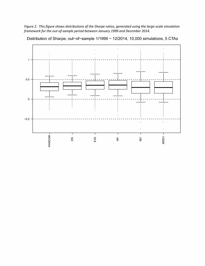
Figure 2. This figure shows distributions of the Sharpe ratios, generated using the large-scale simulation framework for the out-of-sample period between January 1999 and December 2014.

Figure 3. This figure shows distributions of the Calmar ratios, generated using the large-scale simulation framework for the out-of-sample period between January 1999 and December 2014.

Figure 4. This figure shows distributions of the Fung-Hsieh (2001) five-factor t-statistic of alpha, generated using the large-scale simulation framework for the out-of-sample period between January 1999 and December 2014.

Figure 3

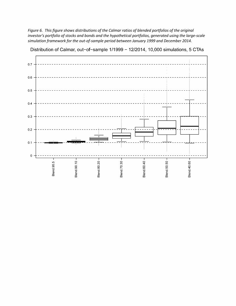
Figure 6. This figure shows distributions of the Calmar ratios of blended portfolios of the original investor's portfolio of stocks and bonds and the hypothetical portfolios, generated using the large-scale simulation framework for the out-of-sample period between January 1999 and December 2014.

Table I. Summary statistics and tests of normality, heteroskedasticity and serial correlation in CTA returns This table reports the statistical properties of fund returns and residuals by strategy and current status. Panel A displays the number of funds in each category and the cross-sectional means of the Fung-Hsieh (2001) five-factor model monthly alpha, t-statistic of alpha, kurtosis and skewness of fund residuals. Panel B reports the percentage of funds for which the null hypothesis of normal distribution is rejected by the Jarque-Bera test, the percentage of funds for which the null hypothesis of homoskedasticity is rejected by the Breusch Pagan test and the percentage of funds for which the null hypothesis of zero first-order autocorrelation is rejected by the Ljung-Box test. All tests are applied to fund residuals and the p-value is set at the 10% level.

Panel A

number

of funds alpha

t-stat of

alpha kurtosis skewness

All Funds 1927 0.43% 0.91 4.27 0.09

By Strategy:

Arbitrage 24 0.05% 0.33 6.33 -0.13

Discretionary 34 -0.06% 0.02 4.30 -0.10

Fundamental - Agricultural 44 0.46% 0.62 5.71 0.41

Fundamental - Currency 97 0.50% 0.97 4.28 0.23

Fundamental - Diversified 105 0.38% 0.95 4.13 0.15

Fundamental - Energy 23 0.03% 0.25 4.60 0.26

Fundamental - Financial/Metals 79 0.24% 0.77 4.70 0.12

Fundamental - Interest Rates 12 -0.10% -0.26 3.21 -0.06

Option Strategies 88 -0.16% 0.04 7.21 -0.43

Stock Index 85 0.14% 0.57 4.35 0.06

Stock Index,Option Strategies 3 -0.86% -1.88 6.43 -1.07

Systematic 39 0.41% -0.53 4.07 0.09

Technical - Agricultural 9 -0.50% -0.72 4.29 0.26

Technical - Currency 203 0.35% 0.74 4.18 0.25

Technical - Diversified 714 0.67% 1.28 3.84 0.09

Technical - Energy 4 -0.54% -0.46 3.89 -0.06

Technical - Financial/Metals 214 0.37% 0.89 3.86 0.03

Technical - Interest Rates 11 0.46% 1.37 3.37 -0.12

Other 139 0.40% 1.10 4.46 0.07

By current status:

Live funds 604 0.71% 1.51 4.26 0.11

Dead funds 1323 0.30% 0.62 4.27 0.08

Mean

Panel B

Test of

normality

Test of

heteroskedasticity

Test of

autocorrelation

Funds

with

Jarque-

Bera p<0.1

Funds with

Breusch Pagan

p<0.1

Funds with

Ljung-Box

p<0.1

All Funds 45% 24% 21%

By Strategy:

Arbitrage 75% 17% 13%

Discretionary 41% 12% 15%

Fundamental - Agricultural 57% 16% 27%

Fundamental - Currency 52% 19% 20%

Fundamental - Diversified 51% 21% 11%

Fundamental - Energy 52% 4% 9%

Fundamental - Financial/Metals 52% 9% 14%

Fundamental - Interest Rates 25% 42% 33%

Option Strategies 80% 43% 22%

Stock Index 41% 25% 15%

Stock Index,Option Strategies 67% 33% 33%

Systematic 46% 13% 23%

Technical - Agricultural 67% 11% 11%

Technical - Currency 46% 14% 22%

Technical - Diversified 38% 28% 22%

Technical - Energy 50% 0% 25%

Technical - Financial/Metals 34% 23% 20%

Technical - Interest Rates 36% 55% 9%

Other 50% 25% 27%

Table II. Performance of a 60-40 portfolio of stocks and bonds for 1999-2014

Annualized Excess Return 3.61%

Annualized StDev 9.59%

Maximum Drawdown 39.29%

Sharpe ratio 0.376

Calmar ratio 0.092

This table reports the annualized excess return, standard deviation, maximum

drawdown, Sharpe ratio and Calmar ratio of the 60-40 portfolio of stocks and bonds for

1999-2014. The portfolio is constructed using S&P 500 Total Return Index and the JP

Morgan Global Government Bond Index. The 3-month Treasury bill (secondary market

rate) is used as a proxy for the risk-free rate. Calmar is the ratio of the annualized excess

return to the maximum drawdown.

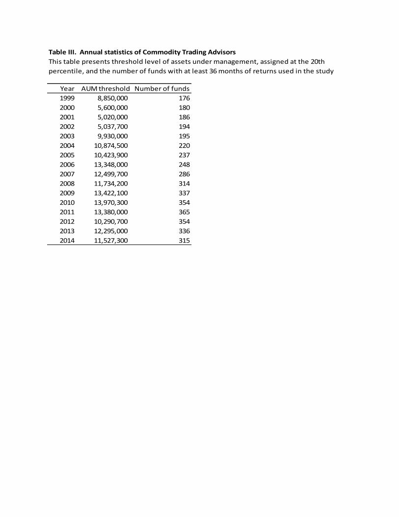
Table III. Annual statistics of Commodity Trading Advisors

Year AUM threshold Number of funds

1999 8,850,000 176

2000 5,600,000 180

2001 5,020,000 186

2002 5,037,700 194

2003 9,930,000 195

2004 10,874,500 220

2005 10,423,900 237

2006 13,348,000 248

2007 12,499,700 286

2008 11,734,200 314

2009 13,422,100 337

2010 13,970,300 354

2011 13,380,000 365

2012 10,290,700 354

2013 12,295,000 336

2014 11,527,300 315

This table presents threshold level of assets under management, assigned at the 20th

percentile, and the number of funds with at least 36 months of returns used in the study

Panel A. Mean values

Portfolio Construction Approach Sharpe Calmar Improvement in Sharpe

Improvement

in Calmar

RANDOM 0.416 0.108 96.58% 98.46%

EN 0.416 0.108 98.60% 99.30%

EVA 0.409 0.104 97.60% 98.28%

RP 0.410 0.105 97.53% 98.14%

MV 0.399 0.100 89.23% 89.64%

MDEV 0.399 0.100 89.14% 89.46%

Panel B. Median values

Portfolio Construction Approach Sharpe Calmar

Improvement in

Sharpe

Improvement

in Calmar

RANDOM 0.415 0.107 96.58% 98.46%

EN 0.416 0.107 98.60% 99.30%

EVA 0.408 0.103 97.60% 98.28%

RP 0.410 0.104 97.53% 98.14%

MV 0.397 0.099 89.23% 89.64%

MDEV 0.397 0.099 89.14% 89.46%

This table reports the results of a marginal contribution analysis. The original investor portfolio is

represented by a 60-40 portfolio of stocks and bonds. It has delivered a Sharpe ratio of 0.376 and a

Calmar ratio of 0.092 over the period 1999-2014. The first column presents the Sharpe ratio of a

blended portfolio that replaces 10% of the allocation to the original portfolio with 10% of the CTA

portfolios constructed in the simulation framework. The second column reports the Calmar ratio

of the blended portfolios. The third and fourth columns report the percentage of time the

blended portfolios have higher Sharpe and Calmar ratios than those of the original portfolio.

Panel A reports mean values, Panel B displays median values.

Table VI. Portfolio contribution of CTA investments to the original

investor portfolio, 1999-2014

Table VII. Sharpe ratios of blended portfolios

Panel A. Percentage of scenarios with higher Sharpe

Portfolio Construction Approach 5% 10% 20% 30% 40% 50% 60%

RANDOM 97.0% 96.6% 95.2% 92.9% 88.6% 82.3% 73.4%

EN 98.7% 98.6% 97.9% 96.6% 93.9% 89.1% 81.6%

EVA 97.9% 97.6% 97.1% 96.1% 94.5% 91.6% 86.8%

RP 97.7% 97.5% 96.8% 95.6% 93.5% 90.4% 84.9%

MV 89.7% 89.2% 87.8% 85.7% 83.5% 79.7% 74.1%

MDEV 89.6% 89.1% 87.9% 85.9% 83.4% 79.7% 74.0%

Panel B. Mean

Portfolio Construction Approach 5% 10% 20% 30% 40% 50% 60%

RANDOM 0.396 0.416 0.454 0.482 0.494 0.487 0.463

EN 0.396 0.416 0.456 0.489 0.507 0.506 0.487

EVA 0.392 0.409 0.443 0.477 0.504 0.519 0.516

RP 0.393 0.410 0.447 0.482 0.509 0.522 0.517

MV 0.387 0.399 0.425 0.450 0.472 0.485 0.483

MDEV 0.387 0.399 0.424 0.449 0.470 0.483 0.480

Panel C. Median

Portfolio Construction Approach 5% 10% 20% 30% 40% 50% 60%

RANDOM 0.396 0.415 0.453 0.482 0.493 0.486 0.460

EN 0.396 0.416 0.456 0.488 0.506 0.504 0.483

EVA 0.391 0.408 0.442 0.475 0.502 0.517 0.513

RP 0.392 0.410 0.445 0.480 0.508 0.520 0.515

MV 0.386 0.397 0.420 0.444 0.464 0.477 0.475

MDEV 0.386 0.397 0.420 0.443 0.463 0.475 0.474

Allocation to CTA portfolios

This table reports the performance of the blended portfolios for 1999-2014. Panel A reports

the percentage of scenarios in which the Sharpe ratio of the blended portfolio exceeds the

Sharpe ratio of the investor's original portfolio. Panel B reports the cross-sectional mean of

the Sharpe ratios of the blended portfolios. Panel C reports the cross-sectional median of

the Sharpe ratios of the blended portfolios.

Table VIII. Calmar ratios of blended portfolios

Panel A. Percentage of scenarios with higher Sharpe

Portfolio Construction Approach 5% 10% 20% 30% 40% 50% 60%

RANDOM 98.5% 98.5% 98.0% 97.0% 95.9% 94.2% 91.6%

EN 99.3% 99.3% 99.1% 98.8% 98.1% 97.1% 95.7%

EVA 98.3% 98.3% 98.2% 98.0% 97.6% 96.7% 95.5%

RP 98.1% 98.1% 98.0% 97.7% 97.0% 96.1% 94.8%

MV 89.6% 89.6% 89.3% 88.1% 86.2% 84.0% 81.0%

MDEV 89.5% 89.5% 89.1% 87.9% 86.2% 83.9% 81.3%

Panel B. Mean

Portfolio Construction Approach 5% 10% 20% 30% 40% 50% 60%

RANDOM 0.099 0.108 0.128 0.153 0.182 0.211 0.224

EN 0.099 0.108 0.129 0.154 0.186 0.220 0.240

EVA 0.097 0.104 0.120 0.139 0.164 0.195 0.225

RP 0.098 0.105 0.121 0.142 0.167 0.199 0.228

MV 0.095 0.100 0.110 0.122 0.136 0.153 0.172

MDEV 0.095 0.100 0.110 0.122 0.136 0.152 0.171

Panel C. Median

Portfolio Construction Approach 5% 10% 20% 30% 40% 50% 60%

RANDOM 0.099 0.107 0.127 0.150 0.176 0.199 0.207

EN 0.099 0.107 0.128 0.152 0.181 0.210 0.225

EVA 0.097 0.103 0.119 0.137 0.160 0.186 0.212

RP 0.098 0.104 0.121 0.140 0.163 0.190 0.214

MV 0.095 0.099 0.109 0.119 0.130 0.142 0.154

MDEV 0.095 0.099 0.109 0.119 0.130 0.142 0.154

This table reports the performance of the blended portfolios for 1999-2014. Panel A reports

the percentage of scenarios in which the Calmar ratio of the blended portfolio exceeds the

Calmar ratio of the investor's original portfolio. Panel B reports the cross-sectional mean of

the Calmar ratios of the blended portfolios. Panel C reports the cross-sectional median of

the Calmar ratios of the blended portfolios.

Allocation to CTA portfolios