A simulation analysis of the fate of phytoplankton

within the Mid-Atlantic Bight

(NASA-CB-177265) A SIMULATION ANALYSIS OF N86-26670THE FATE OF - P H Y 10PLANK1CN WITHIN THEMID-ATLANTIC EIGHT {0Diversity of Soutiflorida, St..Petersburg.) 62 p OnclasHC A04/HF A01 CSCL 08A G3/43 43604

by

John J. Walsh, Dwight A. Dieterle, and Mark B. Meyers

Department of Marine Science

University of South Florida .

St. Petersburg, Florida 33701

https://ntrs.nasa.gov/search.jsp?R=19860017198 2018-06-23T08:07:39+00:00Z

ABSTRACT

A time-dependent, three-dimensional simulation model of

wind-induced changes of the circulation field, of light and nutrient

regulation of photosynthesis, of vertical mixing as well as algal

sinking, and of herbivore grazing stress, is used to analyze the

seasonal production, consumption, and transport of the spring bloom

within the mid-Atlantic Bight. Our case (c) of a 58-day period in

February-April 1979, simulated primary production, based on both

-2 -1nitrate and recycled nitrogen, with a mean of 0.62 g C m day over

the whole model domain, and an export at the shelf-break off Long

- 2 - 1Island of 2.60 g chl m day within the lower third of the water

column. About 57% of the carbon fixation was removed by herbivores,

with 21% lost as export, either downshelf or offshore to slope waters,

after the first 58 days of the spring bloom. Extension of the model

for another 22 days of case (c) increased the mean export to 27%,

while variation of the model's parameters in 8 other cases led to a .

range in export from 8% to 38% of the average primary production.

Spatial and temporal variations of the simulated algal biomass, left

behind in the shelf water column, reproduced chlorophyll fields sensed

by satellite, shipboard, and in situ instruments.

\

INTRODUCTION

Satellite time series of the 1979 spring bloom within the

mid-Atlantic Bight (WALSH, DIETERLE and ESAIAS, 1987a) and moored

fluorometer time series of the 1984 spring bloom in the same region

(WALSH, WIRICK, PIETRAFESA, WHITLEDGE, HOGE and SWIFT, 1987b)

suggested that the daily export of algal biomass to slope waters might

-2 -1be 1.8-2.7 g chl m day across the shelf-break. Such time series

lacked depth resolution, however, since the CZCS sampled, at most, the

upper 10 m of the water column and the in situ instruments sampled

perhaps the lower 5 m at the 80 m and 120 m isobaths. Furthermore,

the algal biomass detected by the CZCS over space and by the moored

fluorometer over time only represented what was left behind in the

water column by the bacteria, zooplankton, and benthos of this shelf

ecosystem.

To place these daily estimates of export in the context of

seasonal production, consumption, and transport of the spring bloom, a

simulation model of the plankton dynamics, over 6000 grid points in

the horizontal plane and 3 depth layers in the vertical, was run for

58 days from 28 February to 27 April 1979 in response to wind-induced

changes of the barotropic circulation field. The details of the

time-dependent terms for the physical circulation, for the light and

nutrient regulation of photosynthesis, for the vertical mixing, for

the algal sinking, and for the grazing stress at -18000 grid points

are discussed below.

During the 6 yr interval between these CZCS and fluorometer time

series, a set of biochemical surveys was also conducted each April

aboard the R/V Kelez, Advance II, and Cape Henlopen. The April

8 «

7 .

6

5

4

3

2 -

I

1979 I960 1981 1982 1983 1984

Figure 1. The mean chlorophyll content (mg m'3) of surface waters(0-30 m) of the mid-Atlantic Bight at 27 stationsre-occupied each April from 1980 to 1984 (W. GREGG,personal communication).

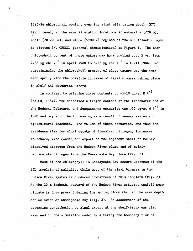
1980-84 chlorophyll content over the first attenuation depth (37%

light level) at the same 27 station locations in estuarine (<20 m),

shelf (20-200 m), and slope (>200 m) regions of the mid-Atlantic Bight

is plotted (W. GREGG, personal communication) as Figure 1. The mean

chlorophyll content of these waters may have doubled over 5 yr, from

2.38 ug chl i'1 in April 1980 to 5.25 ug chl t~l in April 1984. Not

surprisingly, the chlorophyll content of slope waters, was the same

each April, with the possible increase of algal biomass taking place

in shelf and estuarine waters.

In contrast to pristine river contents of -5-10 ug-at N X,

(WALSH, 1984), the dissolved nitrogen content at the freshwater end of

the Hudson, Delaware, and Susquehanna estuaries was >50 ug-at Hi in

1980 and may still be increasing as a result of sewage wastes and

agricultural leachate. The volume of these estuaries, and thus the

residence time for algal uptake of dissolved nitrogen, increases

southward, with consequent export to the adjacent shelf of mainly

dissolved nitrogen from the Hudson River plume and of mainly

particulate nitrogen from the Chesapeake Bay plume (Fig. 2).

Most of the chlorophyll in Chesapeake Bay occurs upstream of the

25X isopleth of salinity, while most of the algal biomass in the

Hudson River system is produced downstream of this isopleth (Fig. 2).

At the 20 m isobath, seaward of the Hudson River estuary, tenfold more

nitrate is thus present during the spring bloom than at the same depth

off Delaware or Chesapeake Bay (Fig. 3). An assessment of the

estuarine contribution to algal export at the shelf-break was also

examined in the simulation model by altering the boundary flux of

2

SALINITY (%.)

15 25 35

SALINITY (%.)

5 15 25\ i i r^

o-o WINTER\ X »r-» SUMMER

K*,.

35

i I

\

SALINITY (%.)

15 25I I r T

o-o WINTERx--x SUMMER

100

60

60

40

20

0

A)HUDSON B) DELAWARE C)CHESAPEAKE

i l io—o WINTER

x—x SUMMER

15 25

SALINITY (%,)

o—o WINTERx—x SUMMER

I Io—o WINTERx~x SUMMER

SALINITY (%.)

15 25

SALINITY (%.)

35

100

8O

60

40

20

0

Figure 2. The nitrate and chlorophyll distributions within thea) Hudson, b) Delaware, and c) Chesapeake estuaries as apercentage function of their maximum value and salinityduring winter (o) and summer (x) - after CARPENTER et al.,1969; MCCARTHY et al., 1977; DECK, 1981; and SHARP et al.,1982.

nutrients at the mouths of these three estuaries as well as that from

Long Island Sound (Fig. 4).

METHODS

1. Circulation

Ignoring tidal forces and the horizontal stress terms of the

Navier-Stokes equations, their cross-differentiation and the

continuity equation leads to a steady-state, depth-integrated form of

the vorticity equation as

on OTJ OT? 21?,3H 34 3H 3<K ,

Bx By 3y Bx Bx By Bx By

where the first term is a description of vortex shrinking or

stretching as a water parcel crosses an isobath, in which H is the

bottom depth, and <)> is the sea level potential, defined as the product

of the acceleration of gravity and the height of the free surface

elevation. The second and third terms are respectively the curl of

the components of the bottom stress, B and B , and of the windy x

forcing, F and F in a left-hand cartesian coordinate system, with zy x

positive downwards.

The bottom stress can be defined (HOPKINS and DIETERLE, 1983) in

terms of the sea level potential and the wind stress by

MARCH APRIL MAY JUNE JULY AUGUST SEPTEMBER

C)CHESAPEAKE N03

20 \-

-HO

-4 20

MARCH APRIL MAY JUNE JULY AUGUST SEPTEMBER

Figure 3. The seasonal structure of nitrate (pg-at IT1) at the 20 misobath off the a) Hudson, b) Delaware, and c) Chesapeakeestuaries during March-September (T. WHITLEDGE, personalcommunication).

where b- and b~ represent that portion of the bottom stress due to the

wind-driven velocity components. In waters deeper than the surface

Ekman layer (H £ 30 m), the bottom stress terms become similar to

those of HSUEH and PENG (1978), e.g.,

By = a (cos 8) f£+« (sin 6) f± (4)

where 6 is a bottom veer angle, and a represents a scaling depth. It

is somewhat analogous to the depth of the bottom Ekman layer, in which

a might be 5-15 m, with 9 ranging from 0° to 45° (HSUEH and PENG,

1978; HSUEH, 1980; HAN, HANSEN and GALT, 1980; and CSANADY, 1981).

Substituting eqs. (2) and (3) in eq. (1), assuming that the wind

curl is negligible, and setting h = H + a., leads to

,3h 3£ 9h 3£, f ,^3x 3y " 3y 3x; a2 ^2 g 2

} ^3y 3y 3x

3b.

which can be solved as a steady-state, boundary-value problem for the

sea level potential.

Wind forcing also enters the solution of eq. (5), at the coastal

boundary condition, where the depth-integrated transport normal to the

41*. •41'

•4Cf

39"

38'

37*

36

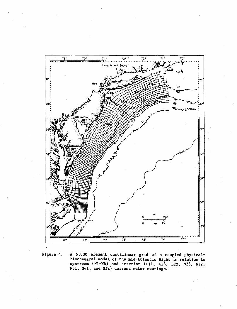
Figure 4. A 6,000 element curvilinear grid of a coupled physical-biochemical model of the mid-Atlantic Bight in relation toupstream (N1-N6) and interior (Lll, L13, LTM, N23, N22,N31, N41, and NJ2) current meter moorings.

IIcoastline, U = / udz, is assumed to be zero, except at the mouths of

tithe three estuaries. The alongshore transport, V = / vdz, at the

coastal boundary (Fig. 4) is governed by the depth-integrated shallow

water equation

3Vwhere all the terms are defined above. At steady-state, i.e., — = 0,dt

eq. (6) becomes

F = B + H (7)y y 9y

except at the estuaries, where U is non-zero. Use of eq. (3) results

in

"y ' " + "2 + "2

at x = 0. For 13 time intervals between 28 February and 27 April

1979, the alongshore component of the mean wind stress observed at

John F. Kennedy airport (Fig. 5) was entered in the simulation, with a

new steady-state solution of <J> calculated (HOPKINS and DIETERLE, 1983)

at each grid point (Fig. 4) from a finite difference form of eqs. (5)

and (8).

The open water boundary conditions for <J> must also be specified,

of course, for solution of this boundary value problem. The sea

WIND STRESS-JFK(DYNES/CM2)

-5 -1- I M I t I I M I M M M I I I I I I M ( I M I I M I I M I I M I I I M I I I I M M I I M t M I M )25 1 5 10 15 20 25 15 10 15 20 25 1FEB MflR flpR MflY

Figure 5. The daily and mean wind stress (dynes cm"2) over 13periods as measured at the John F. Kennedy airport between25 February and 1 May 1979.

elevation at the upstream boundary of the grid was computed from the

observed currents (BEARDSLEY, CHAPMAN, BRINK, RAMP and SCHLITZ, 1985)

at Nl to N5 (Fig. 4) for each time interval (Fig. 5). Since the April

1979 currents were mainly barotropic in the mid-Atlantic Bight

(HOPKINS and DIETERLE, 1987) and hydrographic data on density

gradients were sparse, we did not attempt to subtract the baroclinic

component of flow from the current meter records. At the offshore

boundary, sea elevation was set to a constant 5 cm, i.e., mass

exchange was confined at the shelf-break to the surface and bottom

32d>Ekman layers. At the downstream boundary (Fig. 4), •=—* = 0 wasdy

specified (HSUEH, 1980).

At each point of the curvilinear grid (HOPKINS and DIETERLE,

1983) of the model, i.e., a length of 886 km alongshore at the coast

and 676 km at the shelf-break (Fig. 4), <J> was first computed for each

of the 13 wind cases and then inserted in the steady-state Ekman

equations

f + fv (9)z 9z2

= K _y. - fu do)9y Z 2

for evaluation of u and v. Analytical solution of eqs. (9) and (10)

then allowed (HOPKINS and SLATEST, ,1986) continuous depth resolution

of the flow field for different values of the wind stress and vertical

eddy diffusivity, K , at each steady state. In the biochemicalZ

calculation of eqs. (11) and (12), u and v were entered as the mean of

their depth integral over each of three vertical layers, where the

depth, Z, of a layer varied across the shelf as a function of the

bottom depth, H, i.e., Z = H/3.

2. Light and nutrient regulation

The spatio-temporal distributions of nitrate (N) and chlorophyll

(M) were calculated from

3N 3N 3N 9N . v 32NK = ~ U 3 x - ~ V By"' W^ + Kz7^

O Z

3M 3M 3M 3M . v 32M . M 3MK = - u 3x- - v 3- - w si + Kz 2 + £M - ws al -

where u and v are the horizontal velocities, w is the vertical

velocity derived from the continuity equation, K is the vertical eddyZ

or mixing coefficient discussed below, b is the nitrate/chlorophyll

ratio of 0.5, e is the phytoplankton growth rate described in this

section, w is the sinking rate of the phytoplankton, and g is thes

grazing loss rate to herbivores.

In this simulation analysis, we were concerned with the amount of

phytoplankton export from the mid-Atlantic shelf, which depends on the

amount of "new" dissolved nitrogen added from the slope and estuarine

boundaries (EPPLEY and PETERSON, 1980; WALSH, 1981), not the recycled

production based on ammonium or urea regenerated within the shelf

ecosystem. We thus did not consider the growth of phytoplankton in

eq. (.12) from excretory products (WALSH, 1975), implicit within the

grazing loss term.

The input of nitrate from the coastal boundary was assumed to be

10.0 ug-at N03 X,"1 from the Hudson River, 1.3 ug-at N03 i~

l from

Chesapeake Bay, 1.0 ug-at N0_ 8, from Delaware Bay, and 1.0 ug-at N0_

8, from Long Island Sound. Most of the model's cases assumed that

the nitrate boundary condition of slope water and of upstream shelf

water was 6.0 ug-at N0» I throughout the water column. The

estuarine boundary conditions of nitrate were later increased tenfold

for the eutrophication case, while in two simulation runs the upstream

nitrate content was set instead to 1.0 ug-at NO- fc .

The specific growth rate (hr ) of the p

function of ambient light (I) and nitrate (N)

The specific growth rate (hr ) of the phytoplankton, e, was a

- I/I ) M

where E was the maximum growth rate of 0.026 hr , assuming a mean

temperature of 5°C and a phytoplankton assemblage of 50% netplankton

(MALONE, 1982). The saturation light intensity, I , of STEELE'ss_2 _ i

(1962) inhibition expression was taken to be 5 cal cm hr (MALONE,

1977). The Michaelis half-saturation constant, n, of the nutrient

limitation term (CAPERON, 1967), at which e = em/2, was taken to be

1 ug-at N0_ «. for coastal phytoplankton species (CARPENTER and

GUILLARD, 1971). The depth integral of ambient light over each of the

3 layers was actually a time-dependent function of season, day length,

diel periodicity, and algal biomass.

8

Such a complex light field was described by

-(k + k )z - k MdzJ-l(z,D,t) = 51 sin [ir(t - a)/i(D)]e w s P Jo (14)

where the seasonal light variation in the model was first described

(NAGLE, 1978) as a cosine function of incident radiation (I ) at theo

winter solstice, I (120 g cal cm day ), at the summer solstice, Is

-2 -1(500 g cal cm day ), and the Julian date, D, of the 58-day

simulation,

I (D) = IW + 0.5(IS - IW)[1 - cos 2ir(D - 356)/365] (15)o o o o

The changing photoperiod, or day length, was similarly described by

= iw + 0.5(is - iw)[l - cos 2ir(D - 356)/365] (16)

where iw = 9.1 hr and is =15.6 hr (NAGLE, 1978). The

photosynthetically active radiation (PAR) at depth is about 50%, of

which 15% might be lost as a result of albedo, such that 6 was taken

to be 0.425 in this model.

With specification of the day length, input of total radiation to

the sea surface, and % transmission of 400-720 run wavelengths, the

hourly change of solar irradiance with time, t, can be expressed

(IKUSHIMA, 1967) as

IQ(t) = Im sin3[Ti(t - a)/i(D)] (17)

_2where I is the maximum light intensity at local noon (g cal cm

hr ) for that Julian day, D, and a is the time of sunrise. The solar

irradiance for the day is

IQ(D) = / Im sinJ[TT(t - a)/i (D)] dt (18)o

and was used to obtain I in eq. (17), after solution of eqs. (15) and

(16) for each simulated day of the model.

Finally, the integrated light field for algal photosynthesis over

the depth interval, Z, was computed from the self-shading, exponential

term of eq. (14), where the total extinction coefficient has been

partitioned into those for water, k ; detritus, k ; and phytoplankton,Vi S

k . The specific attenuation coefficient for plant pigments was

assumed to be 0.020 m2 mg"1 chl a (BANNISTER, 1974; JAMART, WINTER,

BANSE, ANDERSON and LAM, 1977). The water and detrital contribution

to water clarity, k + k = 0.13 m , was derived as the averagew s

residual from the observed extinction coefficient and pigment

concentration during 15-24 March 1979 (WALSH et al., 1987a).

Initial conditions of the spatial chlorophyll field of eqs. (11),

(12), and (14) were obtained from a CZCS image of the mid-Atlantic

Bight on 28 February 1979 (SYSTEMS AND APPLIED SCIENCES CORPORATION,

1984), at about the same spatial resolution as the model's grid

(Fig. 4). The 1.0 yg I surface isopleth of chlorophyll was located

10

near the 20 m isobath, and the 0.5 ug 2, isopleth at the 60 m

isobath, with the assumption of uniform pigment distribution within

the 3 vertical layers of the model. The estuarine boundary conditions

of algal biomass were respectively 7.5, 5.0, 4.0, and 3.0 yg chl I

from the Hudson River, Delaware Bay, Long Island Sound, and Chesapeake

Bay. The chlorophyll contents of inflowing shelf and slope waters

were instead set to 0.5 and 0.2 yg chl % at the upstream and

offshore boundaries.

Since Z was a function of the bottom depth, the upper layer of

the model was 10 m deep at the 30 m isobath and 30 m deep at the 90 m

isobath as a result of entering the known bottom topography, H, every

~3 km in the model. The observed depth of the euphotic zone in the

mid-Atlantic Bight during March ranges, however, from about 10 m in

the Hudson River plume (MALONE, HOPKINS, FALKOWSKI and WHITLEDGE,

1983) to -30 m at the shelf-break (WALSH et al., 1987a). Thus a

surface layer of variable depth (as well as the middle and bottom

layers) in the model mimics fairly well the spatial changes of

biological processes across the shelf.

3. Vertical mixing

Time series of CZCS images and vertical profiles of chlorophyll

in March-April 1979 and 1984 (WALSH et al., 1987a; WALSH et al.,

1987b) implied a downward displacement and/or sinking rate of 20-40 m

day for biogenic particles. Using a one-dimensional model (NIILER,

1975) of the wind-induced mixed layer, WROBLEWSKI and RICHMAN (1986)

2 - 1 2computed a vertical eddy coefficient, K , of 68 m hr (188 cm

11

sec ) over a 44 m deep mixed layer of weak vertical stratification

(0.35 ofc 50 m" ), after 8.5 hr of a 10 m sec" wind forcing. The

2 ~1 2 -1decay time for a return of K to 8 m hr (22 cm sec ) was of thez

same order of 24 hr after cessation of the wind impulse.

During February-May 1979-82, a wind event £10 m sec occurred

about every 8 days in the mid-Atlantic Bight and at 27 shelf stations,

during 16-24 March 1979, the vertical density gradient was a mean of

0.33 o 52 m . Over a 44 m surface mixed layer in the mid-Atlantic

2Bight, the equivalent vertical displacement rate from a K of 68 m

Z

hr would be 37.1 m day during such March wind events. We wished

to distinguish, however, between downwelling, i.e., w of eqs. (11) and

(12), vertical mixing, i.e., K , and sinking of phytoplankton, i.e.,

w .s

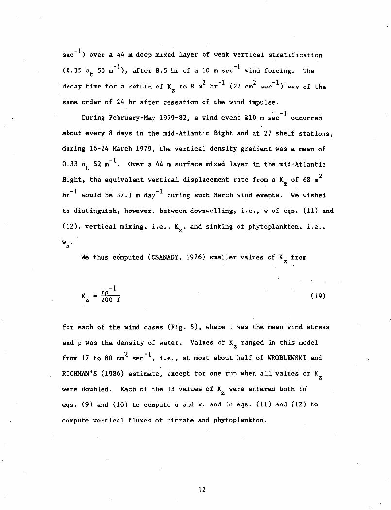
We thus computed (CSANADY, 1976) smaller values of K fromZ

for each of the wind cases (Fig. 5), where T was the mean wind stress

and p was the density of water. Values of K ranged in this modelZ

from 17 to 80 cm2 sec"1, i.e., at most about half of WROBLFAfSKI and

RICHMAN'S (1986) estimate, except for one run when all values of KZ

were doubled. Each of the 13 values of K were entered both inz

eqs. (9) and (10) to compute u and v, and in eqs. (11) and (12) to

compute vertical fluxes of nitrate arid phytoplankton.

12

CHESAPEAKE Jff m,BAY uR\\^m

31

-0-5 -*5-10 —• 10-15

Figure 6. The simulated velocity fields (cm sec"1) of the upper a)and lower b) thirds of the water column under a windforcing of 0.63 dynes cm"2 from 063°T during 1-5 April1979.

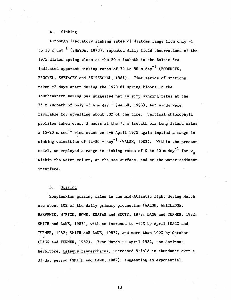
4. Sinking

Although laboratory sinking rates of diatoms range from only ~1

to 10 m day" (SMAYDA, 1970), repeated daily field observations of the

1975 diatom spring bloom at the 80 m isobath in the Baltic Sea

indicated apparent sinking rates of 30 to 50 m day" (BODUNGEN,

BROCKEL, SMETACEK and ZEITZSCHEL, 1981). Time series of stations

taken -2 days apart during the 1978-81 spring blooms in the

southeastern Bering Sea suggested net in situ sinking rates at the

75 m isobath of only -3-4 m day" (WALSH, 1983), but winds were

favorable for upwelling about 50% of the time. Vertical chlorophyll

profiles taken every 3 hours at the 70 m isobath off Long Island after

a 15-20 m sec wind event on 3-6 April 1975 again implied a range in

sinking velocities of 12-50 m day"1 (WALSH, 1983)'. Within the present

model, we employed a range in sinking rates of 0 to 20 m day for w

within the water column, at the sea surface, and at the water-sediment

interface.

5. Grazing

Zooplankton grazing rates in the mid-Atlantic Bight during March

are about 10% of the daily primary production (WALSH, WHITLEDGE,

BARVENIK, WIRICK, HOWE, ESAIAS and SCOTT, 1978; DAGG and TURNER, 1982;

SMITH and LANE, 1987), with an increase to -40% by April (DAGG and

TURNER, 1982; SMITH and LANE, 1987), and more than 100% by October

(DAGG and TURNER, 1982). From March to April 1984, the dominant

herbivore, Calanus finmarchicus, increased 8-fold in abundance over a

33-day period (SMITH and LANE, 1987), suggesting an exponential

13

NEW YORK

•- "*- X€^VN\

DELAWAREBAY

CHESAPEAKE," ( * \*BAY N ' ' '

, ^ .i*i'. '• rr-.'' '::

-0-5 —5-10 —»10-15 —»15+

Figure 7. The simulated velocity fields (cm sec"1) of the upper a)and lower b) thirds of the water column under a windforcing of 1.07 dynes cm"2 from 296°T during 5-12 April1979.

increase of this herbivore population, with a doubling time of about

10 days.

In this model, we thus mainly employed an exponential increase of

the grazing stress, gM, from 28 February to 27 April by using

g = ln(l - G)/[24 - i(D)] (20)

where G was 0.03 e"°-023(59 " D' for H > 50 m, while G was a constant

0.06 for H < 50 m, i.e., there was a spatial gradient of grazing

pressure. To simulate diurnal migration of the copepod grazers, this

grazing stress was only imposed on the phytoplankton of .the upper and

middle layers of the model at night. In terms of primary production,

the exponential grazing stress led to a loss of about 10% of the daily

growth increment in February and 100% at the end of April, i.e.,

losses to benthos and bacterioplankton were then represented by this

term as well. In one experiment of this model, no grazing stress was

assumed, while in another experiment, a linear increase in grazing

stress from March to April of G = 0.1 + 0.0078(D - 69), for D > 69,

was instead applied.

6. Computation

The circulation sub-model was solved by Gaussian elimination

(EISENSTAT, SCHULTZ and SHERMAN, 1976), with the steady-state values

of u, v, w, and K entered in eqs. (11) and (12) for the 13 timez

intervals (Fig. 5). Information about N and M was then obtained, not

from deduction (CHRISTIE, 1941), but from numerical solution. The

time -dependent solutions of the biochemical state equations were thus

14

NEW YORK

DELAWAREBAY

CHESAPEAKEBAY

Figure 8. The simulated chlorophyll (ug IT1) of case (c) within theupper a) and lower c) layers, as well as nitrate (ug-atI'1) in b) the upper layer, on 3 March 1979.

obtained over a staggered grid of the same dimensions of the

circulation model (Fig. 4), with an upstream or "donor cell" finite

difference in space (ROACHE, 1976). Integration over time was done

with a semi-implicit method for the vertical diffusion term and an

explicit, forward in time, differencing method for the other terms

(ROACHE, 1976).

RESULTS

The simulated flow fields of the circulation model were compared

(WALSH et al., 1987a) with AOML current meter observations (MAYER, HAN

and HANSEN, 1982) for April 1979 at 8 moorings in the New York Bight

(Fig. 4). During this time period, the barotropic flow was about 90%

of the transport, agreeing with a prior model's currents within a

vector error of only ~1 cm sec and 10° in the New York Bight

(HOPKINS and DIETERLE, 1987). The extension of this circulation model

to the mid-Atlantic Bight has been previously discussed (WALSH et al.,

1987a), and yielded a mean difference between simulated and observed

currents of 3 cm sec velocity and 35° direction during 5-16 April

1979. The results of the biochemical calculations will thus be

stressed in this analysis.

To provide perspective on the biological response to downwelling

and upwelling events, however, the flow fields during 1-5 April

(Fig. 6) and 5-12 April (Fig. 7) are shown for respective wind

-2 -2forcings of 0.63 dynes cm from 063°T and 1.07 dynes cm from 296°T

(Fig. 5). The surface Ekman layer of the model exhibited onshore

flows of 10-15 cm sec (Fig. 6a) during the northeast wind forcing of

1-5 April, for example, while the bottom layer displayed similar

15

NEW YORK

DELAWAREBAY

CHESAPEAKE •)'(BAY V?

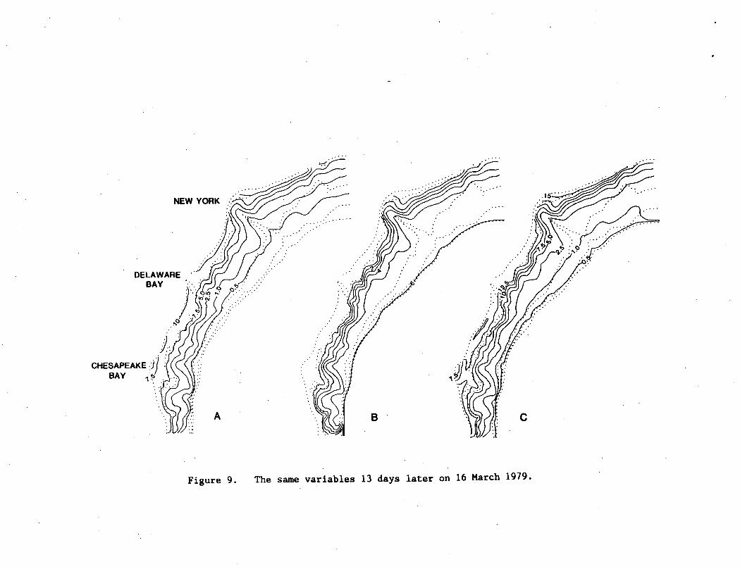
Figure 9. The same variables 13 days later on 16 March 1979.

offshore flow (Fig; 6b), particularly south of New Jersey. The

2 -1vertical mixing coefficient was computed to be 42.7 cm sec during

this time period, with maximum downwelling velocities of 23-26 m day"

on the inner (<30 m depth) and middle (30-60 m depths) parts of the

shelf.

With a shift in wind forcing to the northwest during 5-12 April,

weaker offshore flows of 5-10 cm sec occurred in the surface layer

of the model (Fig. 7a). Onshore flow of 5-10 cm sec then occurred

in the lower layer (Fig. 7b), with maximum upwelling velocities of 9 m

day found on the inner shelf, and as much as 14 m day on the

2 -1middle shelf. A K of 80.9 cm sec , computed during the 5-12 April

case, at the 44 m isobath would yield an effective mixing velocity of

-16 m day to resuspend chlorophyll, if more algal biomass were

located in the lower layer than in the middle or upper layers of the

water column. In this situation, a combination of the calculated Kz

and w, together with an assumed w of 20 m day , would still allow a

vertical input of phytoplankton to the euphotic zone at a net rate of

10 m day

Using a constant sinking velocity of 20 m day and the

time-dependent growth and grazing rates [case (c) of Table 1], we will

describe the seasonal change in biological response to three such

downwelling cases on 3 March, 4 April, and 16 April, and three

upwelling cases on 16 March, 11 April, and 20 April 1979. At the

beginning of March, for example, the incident radiation in the

-2 -1mid-Atlantic Bight was <250 g cal cm day , which, over a well-mixed

water column, would yield a mean in situ light intensity of

16

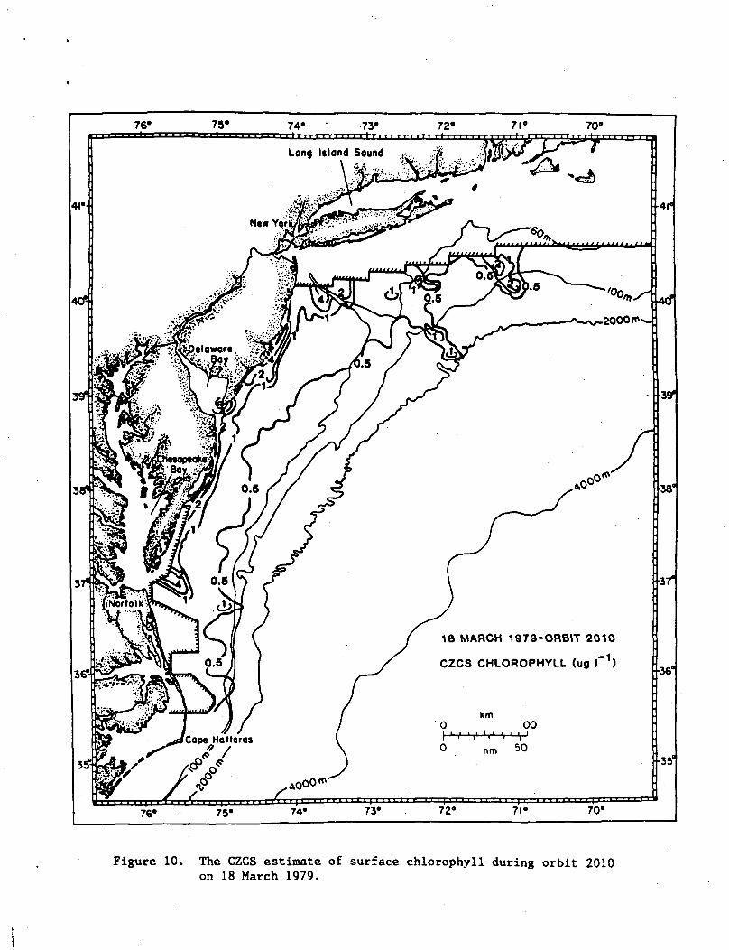
18 MARCH 1979-ORBIT 2010

CZCS CHLOROPHYLL (ug I ')

Figure 10. The CZCS estimate of surface chlorophyll during orbit 2010on 18 March 1979.

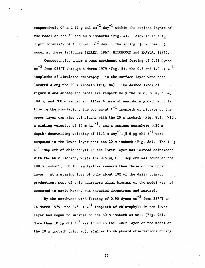
-2 -1respectively 64 and 32 g cal cm day within the surface layers of

the model at the 30 and 60 m isobaths (Fig. 4). Below an in situ

_2 -ilight intensity of 40 g cal cm day , the spring bloom does not

occur at these latitudes (RILEY, 1967; HITCHCOCK and SMAYDA, 1977).

Consequently, under a weak northeast wind forcing of 0.21 dynes

-2 -1cm from 088°T through 4 March 1979 (Fig. 5), the 0.5 and 1.0 yg I

isopleths of simulated chlorophyll in the surface layer were then

located along the 20 m isobath (Fig. 8a). The dashed lines of

Figure 8 and subsequent plots are respectively the 10 m, 20 m, 60 m,

100 m, and 200 m isobaths. After 4 days of nearshore growth at this

time in the simulation, the 5.5 yg-at 1 isopleth of nitrate of the

upper layer was also coincident with the 20 m isobath (Fig. 8b). With

a sinking velocity of 20 m day , and a maximum nearshore (<30 m

depth) downwelling velocity of 11.3 m day , 5.0 yg chl I were

computed in the lower layer near the 20 m isobath (Fig. 8c). The 1 yg

2. isopleth of chlorophyll in the lower layer was instead coincident

with the 60 m isobath, while the 0.5 yg i isopleth was found at the

100 m isobath, -50-100 km farther seaward than those of the upper

layer. At a grazing loss of only about 10% of the daily primary

production, most of this nearshore algal biomass of the model was not

consumed in early March, but advected downstream and seaward.

_2By the northwest wind forcing of 0.90 dynes cm from 287°T on

16 March 1979, the 2.5 yg i~ isopleth of chlorophyll in the lower

layer had begun to impinge on the 60 m isobath as well (Fig. 9c).

More than 10 yg chl I was found in the lower layer of the model at

the 20 m isobath (Fig. 9c), similar to shipboard observations during

17

NEW YORK

DELAWAREBAY

CHESAPEAKEBAY

Figure 11. The simulated chlorophyll (ug 8,'1) of case (c) within theupper a) and lower c) layers, as well as nitrate (pg-atJT1) in b) the upper layer, on 4 April 1979.

24 March 1979 (WALSH et al., 1987a). With this upwelling circulation

- 1 2 - 1of 10-14 m day and a strong mixing coefficient of 74.2 cm sec ,

the 0.5 yg I isopleth of surface chlorophyll occurred at the 60 m

isobath (Fig. 9a), similar to the spatial pattern detected on 18 March

1979 during CZCS orbit 2010 (Fig. 10). After two weeks of growth in

the model, the nearshore dissolved nitrogen stocks were depleted, with

the 1 ug-at £ isopleth of surface nitrate found at the 20 m isobath,

and the 5.5 ug-at £~ isopleth at the 60 m isobath (Fig. 9b).

Subsequent generations of phytoplankton within shallow waters (<20 m

depth) would now grow in the model under nutrient limitation, since

the ambient nitrate concentrations here were less than the

half-saturation constant -- recall eq. (13).

After a month of increasing solar radiation, the in situ light

intensity within the upper 30 m at the 90 m isobath was >40 g cal

_2'~cm in early April, while the nitrate concentration was still

5.5 yg-at N0_ £ here (Fig. -lib). The daily grazing stress was now

about 20% of the outer shelf production, however, and as much as 50%

of the inner shelf production. Within another downwelling

circulation on 4 April, i.e., analogous to 3 March, a uniform algal

biomass of >3 yg chl £ occurred in surface waters, landward of the

50 m isobath (Fig. lla).

Within the lower layer of the model, which reflects the history

of the surface primary production, a mid-shelf maximum of >10 yg chl

£ instead occurred between the 20-60 m isobaths on 4 April

(Fig. lie). With less than 0.5 yg-at N03 £-1 found landward of the

20 m isobath, except for the estuarine discharge, the dissolved source

18

NEW YORK

DELAWAREBAY

CHESAPEAKEBAY

Figure 12. The same variables 7 days later on 11 April 1979.

of particulate nitrogen, sinking out of the surface to nearshore

bottom waters, had been curtailed by this time in the spring bloom.

The mid-shelf maximum of the model on 4 April 1979 was also the result

of prior offshore advection of uneaten phytoplankton from shallow

waters. A near-bottom maximum of >20 ug chl fc was found at

mid-shelf on the 50-60 m isobaths during a 1-5 April 1984 cruise

(WALSH etal., 1987b).

A strong upwelling circulation of 9-14 m day by 11 April 1979

(Fig. 7) led to a simulated resuspension of chlorophyll from this

bottom layer (Fig. 12c) to the top layer (Fig. 12a) at mid-shelf off

New Jersey to Virginia, and immediately south of Long Island. The

lower layer of the model was depleted of chlorophyll, while the upper

layer was enhanced. Thus in situ growth within the euphotic zone

may not have accounted for all of the surface increment of

chlorophyll, calculated at mid-shelf between April 4 and 11

(Fig. 12a).

Similar mid-shelf maxima of surface algal biomass (Fig. Ha) had

been detected aboard ship in April 1975 (WALSH et al., 1978) and

during orbit 2452 of the CZCS on 19 April 1979 (WALSH et al., 1987a).

Although nutrient-rich water was advected shoreward within the aphotic

zone (Fig. 7) in response to upwelling favorable winds (Fig. 5), the

nitrate content of the upper layer at mid-shelf was actually reduced

by ~1 yg-at NCL X."1 between April 4 (Fig. lib) and 11 (Fig. 12b). At

a nitrate/chlorophyll ratio of 0.5, about 40-50% of the primary

production, i.e., biomass increment + grazing loss, was the result of

particulate incorporation of dissolved nitrate.

19

NEW YORK

CHESAPEAKE ABAY ()

0.5

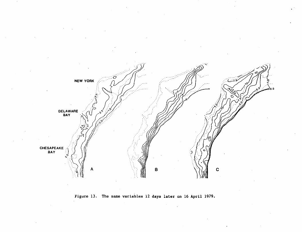
Figure 13. The same variables 12 days later on 16 April 1979.

Another reversal of the winds from the northeast yielded the

third downwelling case of the model by 16 April 1979, with a K ofz

2 -1only 31.2 cm sec , but a maximum downward entrainment velocity of

22-30 m day . High chlorophyll (>10 ug 1 ) was again found within

the bottom layer south of Long Island and at mid-shelf, from New

Jersey to Delaware (Fig. 13c). In contrast to the second downwelling

case of 4 April (Fig. lla), however, a mid-shelf maximum of 2.5 ug chl

8, was simulated by 16 April in the surface layer of the model

(Fig. 13a), with plumes of chlorophyll extending off the Hudson and

Delaware estuaries. These were also observed by the CZCS during

orbit 2425 on 17 April 1979 (Fig. 14). Perhaps as a result of an

apparent lack of surface export of chlorophyll from the Chesapeake

estuary (Fig. 13a), the chlorophyll content of the model's lower layer

at mid-shelf off Virginia on 16 April (Fig. 13c) was less than that on

4 April (Fig. lie).

-2The third upwelling case, of 0.58 dynes cm on 20 April 1979

from 341°T, was the weakest northwest wind forcing, with maximum

positive vertical velocities in the model of only 6-13 m day , and a

2 - iK of 35 cm sec . At the 44 m isobath, such an upwelling rate ofZ

6 m day and an effective mixing rate of only 7 m day would

actually result in a net downward algal transfer of 7 m day , with

the assumed sinking rate of 20 m day . The simulated surface nitrate

pattern on 20 April (Fig. 15b) was quite similar to both the previous

upwelling event on 11 April (Fig. 12b) and the preceding downwelling

case on 16 April (Fig. 13b), indicating little flux of nitrate to the

euphotic zone.

20

Long Island Sound

17 APRIL 1979-ORBIT 2425

CZCS CHLOROPHYLL (ug I )

Figure 14. The CZCS estimate of surface chlorophyll during orbit 2425on 17 April 1979.

A chlorophyll plume of >2.5 ug i , derived from the Hudson River

export, was found in the upper layer of the model off New York

(Fig. 15a), with local maxima of the same amount of algal biomass

found at mid-shelf, farther to the south. The higher biomass

simulated previously by the model in the second upwelling case on

11 April (Fig. 12a) and observed by the CZCS during orbit 2452 on

19 April 1979 (WALSH et al., 1987a), was not reproduced by this

version of the model. Part of the chlorophyll increase detected by

the CZCS on 19 April may have been the result of surface export of

macrophytes from coastal marshes, rather than just resuspension of

near-bottom phytoplankton residues. A lower algal sinking rate of 1 m

day in the model would have yielded a bloom, of course, in this

region of the shelf.

Over the 58-day period of this particular simulation of the 1979

spring bloom, the phytoplankton export was a mean, over 325 km long

-2 -1segments at the shelf-break, of 1.30 g chl m day between Long

-2 -1Island and New Jersey, 2.25 g chl m day between New Jersey and

- 2 - 1Maryland, and 3.64 g chl m day between Maryland and Cape Hatteras

(Fig. 4). More than 90% of this export occurred in the lower layer of

the model, as indicated by the time history of simulated algal biomass

at the 80 m isobath, south of Long Island (Fig. 16). This grid point

of the model was adjacent to 1984 fluorometer moorings at the 80 and

120 m isobaths (WALSH et al., 1987b), which exhibited similar records

of chlorophyll fluctuations at depths of 13 m and 75-81 m (Fig. 17).

Note that near-bottom chlorophyll concentrations of >2 pig chl I were

found after Julian day 80 in both the simulated (Fig. 16) and observed

(Fig. 17) time series.

21

NEW YORK

DELAWAREBAY

CHESAPEAKEBAY '

Figure 15. The simulated chlorophyll (ug 8,"1) of case (c) within theupper a) and lower c) layers, as well as nitrate (ug-atIT1) in b) the upper layer, on 20 April 1979.

The ability of this case of our simulation model to replicate

both spatial patterns of chlorophyll detected by the CZCS (Figs. 10,

14), and temporal patterns detected by moored fluorometers (Fig. 17),

-2 -1suggests that a simulated export of 2.40 g chl m day may be a

reasonable time-averaged mean for March-April in the mid-Atlantic

Bight. If we assume that this export occurred at the 120 m isobath,

with 90% in the lower third of the water column, the depth-averaged

-2 -1mean over the whole water column would then be 0.88 g chl m day

The possible range and implication of such an estimate is discussed in

relation to our evaluation of the parameter space of the model.

DISCUSSION

Nine separate cases of this simulation model were run (Table 1),

with, for example, sinking rates of 1 m day (a), 10 m day (b), and

20 m day (c), at an exponential grazing rate, at the normal mixing

rate, and at the normal estuarine or upstream boundary conditions.

The above results were from case (c). In another run, the mixing rate

was doubled (d), with a sinking rate of 1 m day , and the rest of the

parameters unchanged. In a third experiment, the zooplankton grazing

rate was assumed to be zero (e), or to vary linearly with time (f)

rather than as an exponential function, at an intermediate sinking

rate of 10 m day , with the normal mixing rate and boundary

conditions. A fourth experiment increased tenfold the estuarine input

of dissolved nitrogen, at upstream boundary conditions of 6 yg-at N0_

8,'1 (g) and 1 ug-at N0_ X,"1 (h), with a sinking rate of 20 m day , a

exponential grazing rate, and the normal mixing rate. Finally, the

22

§•H4Jffl

(Q

tx,cq

orH

Q)JS•to

<*4O

§•rt4J91

rH

2Q)

!vl

<U

Q)i-HJQ

co0) 4JCX MO U

rH CXCO X

H

mMH 4-1rH )H0) OX CXCO X

w

00C CN

•H WN U)CTJ OLj .- ~\M t—to

CNC

>> Ot-l -HCO 4JE U•H 3M "O

CU Ot .M

O-i

M r^

(0 M0) CO1, w4M O4-) Cw 3a f*l

\J3 CO

Q)C >.

,_j «,™ M^ CO

3 C3 §(A OH «

00C•H CDN 4J

2 cS0 *

00c a)•H 4-1X r r tnjg «

00C rH

•H 0)

M 4-1C CO•H «CO

4Jc0)s•HM0)CXXM

v O - H c ^ i n r ^ - c N O N O o o o

• H r H O r H C N O O O O

in o en \o m m CN C N O N• • • • • • • • •

t H O o O r H O N r > » c T > c ^ o oC N C N r H C N C O r H r H i - H

o \ r H c n o o i r H r H o o m• • • • c^ • • • •

\ o m m v o i m - T c o c o

v r t N C » C N O t - > . C N C O < -* • * • • • • • •

o o o v o o o s r r ^ v o v orH rH tH

X Xt"^ t"^I—* 1— 1

X X X X X X X^^ ^™t ^^ ^^ r^ ^H ^^ ^^ ^^

x x x x x x x x xrH *H rH fH rH rH t J CO rH

rH rH

M

0) cfla, a, a. a, c a) c x c x c xx x x x o c x x xW W W W Z - H W W W

r—5

X X X X X X X X X^H ^H ^H OJ ^^ ^H ^H ^H '"

r H O O r H O O O O O

rH CN rH tH CN CN CN

c f l r O O T 3 C U 4 H O O r C - H

toT3

CNI CM

I

O rC

U

00E 00

CN m

2\

0-60 ' 70 80 90 100' li0

Figure 16. The simulated chlorophyll content (ug i'1) at noon of eachJulian day from 1 March to 27 April 1979 within theupper (--), middle (—), and lower (...) layers of the80 m water column at a grid point, adjacent to the 1984fluorometer moorings, south of Long Island.

last experiment considered an upstream boundary condition of only

1 ug-at N0» I (i), at the normal estuarine flux of nitrogen, the

usual mixing rate, a sinking rate of 20 m day , and an exponential

grazing rate.

10 2With a surface area of the model of 8.52 x 10 m , an upstream

f\ *?

shelf boundary area of 8.95 x 10 m , a downstream shelf boundary area

f i 9 7 9of 2.10 x 10 m , a shelf-break boundary area of 8.85 x 10 m , and an

f\ *7estuarine boundary area of 2.54 x 10 m , the units of Table 1 can be

8converted to total mass fluxes. For example, a mean of 8.9 x 10 g

chl day was produced over all of the mid-Atlantic shelf during

March-April 1979 for case (a) with a sinking rate of 1 m day . An

average of 66% of this synthesized chlorophyll was lost each day to

grazing, while 21% was lost to export, either downshelf or within

slope waters. The remaining 13% had not yet been removed from the

shelf water column by the end of the simulation (Table 1). In

case (e) of no grazing loss (Table 1), 38% of the March-April daily

chlorophyll production was instead lost as physical export past the

shelf and slope boundaries (Fig. 4) over the same time period.

Using a C/chl ratio of 45/1 (MALONE et al., 1983), the mean daily

fixation of carbon, based just on nitrate, would have been 0.47 g C

_2 _i _2 -im day in case (a) and 0.31 g C m day in case (c) of the model

(Table 1). Averaging over upwelling and downwelling wind events, a

-2 -1mean primary production of 0.57 g C m day was actually measured in

the mid-Atlantic Bight (O'REILLY and BUSCH, 1984) during March-April

1977-80 at 66 stations, excluding the observations from the mouths of

the estuaries (WALSH et al., 1987a). Approximately 50% of the spring

23

O - 2CC oo 3 1T n

0 °

-1 4> _I T^ 3

ft 'O — 2OC 0)O H 1•~ '_JI f \0O

75M (BOTTOM LAYER) "*"****~X. .....?"*" X»-» -V" >> -

50 60 70 80 90

FEBRUARY-APRIL 1984 (JULIAN DAY)

120M ISOBATH-

13M (UPPER LAYER) ^ «/"./ \ X ^ i

— -'*"'v— — ~ * — / % T ^ \ ^ ^AN •» **81 M (MIDDLE LAYER) ^J V^^-^ N

50 60 70 80 90

2

C

3

2i

FEBRUARY-APRIL 1984 (JULIAN DAY)

Figure 17. The observed chlorophyll content (yg H"1), afterapplication of a 40-hr low-pass filter, from mooredfluorometers both at a) 13 m and 75 m on the 80 m isobath,and at b) 13 m and 81 m on the 120 m isobath, south ofLong Island from 19 February to 4 April 1984.

bloom's nitrogen demand is met by nitrate off New York (CONWAY and

WHITLEDGE, 1979). The total carbon fixation predicted by the model

-2 -1 -2would thus have been 0.94 g C m day in case (a) and 0.62 g C m

day in case (c), if uptake of recycled nitrogen had been added to

eq. (12).

The productivity difference between these two cases of the model

was the result of increased light limitation, induced by changing the

sinking rate from 1 m day to 20 m day (Table 1) i.e., thereby

decreasing the residence time of an algal cell within the euphotic

zone. In contrast, a doubling of K in case (d) had little impact onz

the production or export of chlorophyll, compared to case (a) in

Table 1. The vertical structure of chlorophyll in cases (a) or (d)

was quite different, however, from case (c), either over time at the

30 m (Fig. 18) and 50 m (Fig. 19) isobaths, south of Delaware, or

within specific spatial patterns in the downwelling (Fig. 20) and

upwelling (Fig. 21) circulation modes.

A sinking rate of 1 m day allowed no vertical structure of

chlorophyll to develop at the 30 m (Fig. 18a) and 50 m (Fig. 19a)

isobaths, adjacent to the Philadelphia dump site at 38°37'N, 74°22'W,

i.e., east of the mouth of Delaware Bay. A uniform 5-6 yg chl I was

then found throughout the whole mid-shelf region within either the

lower layer of a downwelling circulation on 4 April 1979 (Fig. 20al or

in the surface layer during an upwelling event on 11 April 1979

(Fig. 21a), i.e., Julian days 94-106 of Figure 19a. In cases (a) or

(d), the seasonal peak of vertically homogeneous chlorophyll on day 95

at the 50 m isobath (Fig. 19a) followed about two weeks after the

24

12-

9-

6-

3-

0:

12-

9-

12-

9-

6-

3-

B

060 70 80 90 100 110

Figure 18. The simulated chlorophyll content (pg &'1) at noon of eachJulian day from 1 March to 27 April 1979 within theupper (--), middle (—), and lower (...) layers of the30 m water column at a grid point, east of Delaware Bay,of a) case (a), b) case (f), and c) case (g).

maximum algal biomass on day 82 at the 30 m isobath (Fig. 18a), i.e.,

a seaward progression of ~2 km day .

In cases (a) or (d), a peak of 6 ug chl i throughout the water

column was subsequently observed one week later on Julian day 102 at

the 80 m isobath, south of Long Island, as well. This was in contrast

to about 4 ug chl i in the lower layer and 1 yg chl I in the upper

layer of case (c) -- recall Figure 16. Since high values of 6 yg chl

2, were not found during April from this region, either in the 1984

moored fluorometer records (Fig. 17), or within a previous 9-yr data

base of ~5000 stations (Fig. 22), the loss terms of sinking and

grazing within cases (a) and (d) were probably too small.

An increased sinking rate of 10 m day and no grazing loss of

case (e) resulted (Table 1) in the same primary production as

cases (a) and (d). The average April chlorophyll of the lower layer

in case (e) was 11.42 ug I (Table 2), however, about 3-fold that of

cases (a) or (d). The average daily algal export to the slope of the

lower layer of the model past the location of the fluorometer moorings_2 -i

in case (e) also increased to 4.0 g chl m day , compared to an

observed 1984 mean of 2.7 g chl m"2 day"1 (WALSH et al., 1987b). The

computed slope import of case (e) would actually have been 8.0 g chl

-2 -Im day , if recycled nitrogen had been included as a nutrient source

of this model.

A linear grazing stress, which was larger than the exponential

formulation, and the same 10 m day sinking rate of case (f), instead

consumed all of the March-April primary production on a mean basis

(Table 1). The algal biomass above the 30 m (Fig. 18b) and 50 m

25

12-

9-

6-

3-

12-

9-

6-

3-

9-

6-

3-

B

60 70 80 90 100 li0

Figure 19. The simulated chlorophyll content (ug •1) at noon of eachJulian day from 1 March to 27 April 1979 within theupper (--), middle (—), and lower (...) layers of the48 m water column at a grid point, adjacent to thePhiladelphia dumpsite east of Delaware Bay, ofa) case (a), b) case (f), and c) case (g).

(Fig. 19b) isobaths was reduced to zero by Julian day 115 of case (f),

with only 0.5-1.0 jig chl 8, found previously on 4 April (20b) and

11 April (21b) 1979. The average 1979 March-April export at the 80 m

isobath of this third grazing experiment in case (f) was only 0.3 g

-2 -1chl m day , an order of magnitude less than the observed flux in

1984.

The exponential grazing stress and the 20 m day sinking rate of

case (c) thus appeared to be the best combination of loss terms of

this simulation model to approximate prior satellite (Figs. 10, 14),

moored fluorometer (Fig. 17), and shipboard (Fig. 21.) estimates of

chlorophyll. We accordingly used these parameters of the model to

evaluate changes of the boundary fluxes of nutrients within cases (g),

(h), and (i). The lingering 5 ng-at £ concentration of nitrate

across the shelf, south of Martha's Vineyard, in Figure lib, for

example, was an artifact of the time invariant upstream boundary

condition of 6 yg-at NO- i in case (c). A reduction of the upstream

boundary condition to 1 vtg-at N0_ £, (Table 1) in cases (h) and (i)

did not significantly alter the primary production, grazing loss, or

export, however, compared to case (c), and we discuss instead the

results of the eutrophication case (g).

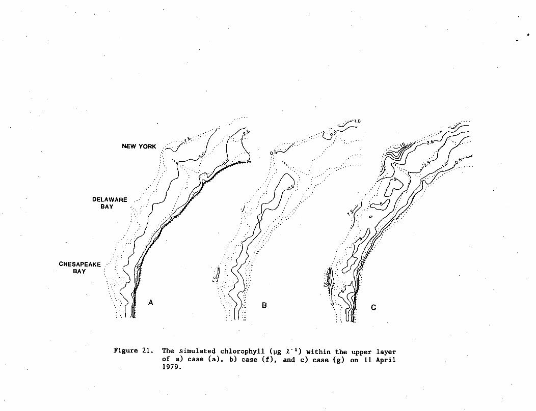
A tenfold increment of the estuarine nutrient loading to the

mid-Atlantic Bight in case (g) significantly increased the nearshore

chlorophyll concentrations of the upper (Fig. 21c) and lower

(Fig. 20c) layers between Cape May and Montauk Point, i.e., the New

York Bight, as well as off Delaware Bay, and off Chesapeake Bay,

compared to the previous results of case (c) in Figures lie and 12a.

26

NEW YORK

DELAWAREBAY

CHESAPEAKEBAY

Figure 20. The simulated chlorophyll (ug J,"1) within the lower layerof a) case (a), b) case (f), and c) case (g) on A April1979.

The algal biomass of case (g) did not increase much either at the 30 m

(Fig. 18c) and 50 m (Fig. 19c) isobaths off Delaware, however, or

within the whole spatial domain of the model (Table 2). The primary

production of the entire mid-Atlantic Bight (Table 1) only increased

by 5% in case (g).

Since the export of estuarine nitrogen to the shelf in case (g)

was still only 10% of that.from the upstream boundary, this result is

not surprising. It does raise the point, however, that compression of

4 x 10 data points in one single spatio-temporal mean for each entry

of Table 1 obscures the spatial and temporal complexity of both this

model and the "real world." Table 1, for example, does not indicate

for case (c) that either 90% of the simulated slope import occurs in

the lower layer of the model, or that the computed slope import off

Virginia is 3-fold that off New York.

Furthermore, the shelf export has a time dependency associated

with the estuarine source function. Extension of this calculation for

case (g) to 20 May 1979, for example, leads to a 25% increase of the

shelf export from the lower layer, since not all of the

estuarine-derived particulate matter had reached the shelf-break by

20 April 1979 in the model. This effect is demonstrated by the first

and second bar graphs of each month in Figure 21, which are the mean

chlorophyll concentrations during 1974-82 in the upper 20 m and the

lower 20-50 m, or 20-75 m, of the New York Bight, while the third and

fourth bar graphs are other chlorophyll means of an independent data

set, taken over the larger area of the mid-Atlantic Bight. During

March, April, and May, the chlorophyll concentrations of the New York

27

Table 2. April 1979 algal biomass (yg chl i~ ) scenarios

Experiment

a

b

c

d

e

f

g

h

i

Upper layer

4.01

2.64

1.81

3.95

6.16

0.25

1.97

1.75

1.59

Middle layer

3.78

3.40

2.90

3.80

8.07

0.33

3.12

2.77

2.54

Lower layer

3.97

4.87

5.20

3.90

11.42

0.48

5.54

4.85

4.50

Water column

3.92

3.64

3.30

3.88

8.55

0.35

3.55

3.12

2.88

NEW YORK

DELAWARE .BAY

CHESAPEAKEBAY

B

Figure 21. The simulated chlorophyll (ug J,"1) within the upper layerof a) case (a), b) case (f), and c) case (g) on 11 April1979.

Bight, from coastal to slope waters, are at least twice that of the

whole mid-Atlantic Bight, reflecting the increased nutrient loading of

the Hudson River (Fig. 3), i.e., simulated in case (g) as Figures 20c

and 21c.

With a decline in nutrient loading from the Hudson River by June

(Fig. 3) and a seasonal increase of the grazing stress, there are no

differences in mean algal biomass between the data sets of the New

York and mid-Atlantic Bights for the months of June to February

(Fig. 21). If a grazing stress was not imposed during a simulated

tenfold increase of nutrient export from the Hudson River during

summer conditions, anoxia, in fact, developed within the New York

Bight (STODDARD and WALSH, 1987). Temporal and spatial changes of

biochemical processes within the mid-Atlantic Bight are thus both

important in determining the fate of primary production within this

shelf ecosystem.

The algal biomass left behind in the water column as a net result

of the birth and death processes of shelf phytoplankton populations

is, by itself, a poor index of the fate of primary production.

Averaging over the whole water column, for example, cases (a)-(d) had

a range in April algal biomass of only 3.30 to 3.92 ng chl I

(Table 2), but the surface content of case (c) was less than half that*

of case (a). The possible twofold increase of April chlorophyll

concentrations between 1980 and 1984 (Fig. 1), can thus be simulated

(Table 2), with a change in the sinking rate of this simple model

(Table 1). Alternatively, the grazing rate in April 1984 might have

been less than in April 1980, as indicated by the results of case (e)

28

14

12

10

r

Q.ocr3O

O<crUJ

M M

COASTAL ZONE(<20m), N= I376AND222 STATION

N

II8

6

4

2

0

8

6

4

2

0

8

6

4

2

0

" MIDDLE SHELF(20-50m), N= 596 AND 528 STATIONS J

i I i i ii I \ i i iOUTER SHELF(50-IOOm), N=7I4 AND624 STATIONS

i i r r \ \ T i i i iUPPER SLOPE(IOO-IOOO m), N= 283 AND 330 STATIONS

Figure 22. Monthly distribution of mean chlorophyll (yg J,"1) withinthe upper 20 m and the lower 20-50 m, or 20-75 m, of thecoastal zone, the middle shelf, the outer shelf, and theslope in the New York Bight (first and second bar graph ofeach month) and the mid-Atlantic Bight (third and fourthgraphs) during 1974-1982 from 4673 stations.

in Table 2. If we had confined the spatial mean of Table 2 to

estuarine waters (<20 m) of case (g), moreover, a tenfold increase of

the nutrient supply would also have led to more than a doubling of the

algal biomass (Figs. 20c and 21c).

The three alternative scenarios of light limitation, nutrient

regulation, and grazing stress are thus each capable of inducing a

2-fold change in algal biomass within the mid-Atlantic Bight

(Table 2). In concert, these processes can lead to more than a

tenfold variation in downstream and offshore shelf export, amounting

to a range of 8% to 38% of the mean March-April primary production

(Table 1). We are pleased that such a relatively simple biochemical

model, coupled to a simple physical model, can both provide insight on

the interaction of these different processes and reproduce chlorophyll

fields sensed by satellite, shipboard, and in situ instruments.

If recycled nitrogen had been included as a state variable,

case (c) would have predicted a mean March-April primary production of

-2 -10.62 g C m day over the whole model domain, with an export of

-2 -12.60 g chl m day from the lower layer of the model off Long

Island. Such biological and physical fluxes of organic matter have

been measured in the mid-Atlantic Bight as well (WALSH et al., 1987a,

b). Additional field experiments will provide a robustness to such

simulation models, which will eventually allow us to predict, rather

than hindcast, the coastal zone's response to continuing perturbations

of eutrophication, overfishing, and climate modification.

29

ACKNOWLEDGEMENTS

This research was funded by the Department of Energy, the

National Aeronautics and Space Administration, and the National

Oceanic and Atmospheric Administration. We particularly wish to thank

our SEEP colleagues for their arduous efforts at sea during the SEEP-I

experiment in 1983-84. In particular, DR. TERRY WHITLEDGE made

available nutrient and chlorophyll data for this analysis.

30

REFERENCES

BANNISTER T. T. (1974) A general theory of steady state phytoplankton

growth in a nutrient saturated mixed layer. Limnology and

Oceanography. 19, 13-30.

BEARDSLEY R. C., D. C. CHAPMAN, K. H. BRINK, S. R. RAMP, and

R. SCHLITZ (1985) The Nantucket Shoals Flux Experiment (NSFE 79).

Part I: A basic description of the current and temperature

variability. Journal of Physical Oceanography. 15, 713-748.

BODUNGEN B., K. BROCKEL, V. SMETACEK and B. ZEITZSCHEL (1981) Growth

and sedimentation of the phytoplankton spring bloom in the

Bornholm Sea (Baltic Sea). Kieler Meeresforschung Sonderheft, 5_

490-60.

CAPERON J. (1967) Population growth in micro-organisms limited by food

supply. Ecology. 48, 715-722.

CARPENTER J. H., D. W. PRITCHARD and R. C. WHALEY (1969) Observations

of eutrophication and nutrient cycles in some coastal plain

estuaries. In: Eutrophication; Causes, Consequences, and

Correctives. National Academy of Science, Washington,

pp. 210-224.

CARPENTER E. J. and R. L. GUILLARD (1971) Interspecific differences in

nitrate half-saturation constants for three species of marine

phytoplankton. Ecology. 52, 183-185.

CHRISTIE, A. M. (1941) N or M? Dodd, Mead & Co., New York, pp. 1-289.

CONWAY H. L. and T. E. WHITLEDGE (1979) Distribution, fluxes, and

biological utilization of inorganic nitrogen during a spring

bloom in the New York Bight. Journal of Marine Research, 37,

657-668.

31

CSANADY G. T. (1976) Mean circulation in shallow seas. Journal of

Geophysical Research. 81, 5389-5399.

CSANADY G. T. (1981) Shelf circulation cells. Philosophical

Transactions of the Royal Society, London, A302, 515-530.

DAGG M. J. and J. T. TURNER (1982) The impact of copepod grazing on

the phytoplankton of Georges Bank and the New York Bight.

Canadian Journal of Fisheries and Aquatic Science. 39, 979-990.

DECK B. L. (1981) Nutrient-element distributions in the Hudson

estuary. Ph.D. Dissertation, Columbia University, pp. 1-396.

EISENSTAT S. C., M. H. SCHULTZ and A. H. SHERMAN (1976) Considerations

in the design of software for sparse Gaussian elimination. In:

Sparse Matrix Computations. J. R. BUNCH and D. J. ROSE, editors,

Academic Press, New York, pp. 1-453.

EPPLEY R. W. and B. J. PETERSON (1980) Particulate organic matter flux

and planktonic new production in the deep ocean. Nature, 282,

677-680.

HAN G. C., D. V. HANSEN and J. A. GALT (1980) Steady state diagnostic

model of the New York Bight. Journal of Physical Oceanography,

10, 1998-2020.

HITCHCOCK G. L. and T. J. SMAYDA (1977) The importance of light in the

initiation of the 1972-1973 winter-spring diatom bloom in

Narragansett Bay. Limnology and Oceanography. 22, 126-131.

HOPKINS T. S. and D. A. DIETERLE (1983) An externally forced

barotropic circulation model for the New York Bight. Continental

Shelf Research, 2, 49-73.

32

HOPKINS T. S. and L. A. SLATEST (1986) The vertical eddy viscosity and

momentum exchange in coastal waters. Journal of Geophysical

Research (in press).

HOPKINS T. S. and D. A. DIETERLE (1987) Analysis of the baroclinic

circulation in the New York Bight with a 3-d diagnostic model.

Continental Shelf Research (in press).

HSUEH Y. (1980) On the theory of deep flow in the Hudson Shelf Valley.

Journal of Geophysical Research, 85, 4913-4918.

HSUEH Y and C. Y. PENG (1978) A diagnostic model of continental shelf

circulation. Journal of Geophysical Research, 83, 3033-3041.

IKUSHIMA I. (1967) Ecological studies on the productivity of aquatic

plant communities, III. Effect of depth on daily photosynthesis

in submerged macrophytes. Botanical Annals, Tokyo, 80, 57-67.

JAMART M., D. F. WINTER, K. BANSE, G. C. ANDERSON, and R. K. LAM

(1977) A theoretical study of phytoplankton growth and nutrient

distribution in the Pacific Ocean off the northwestern U.S.

Coast. Deep-Sea Research, 24, 753-773.

MALONE T. C. (1977) Light-saturated photosynthesis by phytoplankton

size fractions in the New York Bight, U.S.A. Marine Biology, 42,

281-292.

MALONE, T. C. (1982) Phytoplankton photosynthesis and carbon specific

growth: light-saturated rates in a nutrient rich environment.

Limnology and Oceanography, 27, 226-235.

MALONE T. C., T. S. HOPKINS, P. G. FALKOWSKI and T. E. WHITLEDGE

(1983) Production and transport of phytoplankton biomass over the

continental shelf of the New York Bight. Continental Shelf

Research, 1, 305-337.

33

MAYER D. A., G. C. HAN and D. V. HANSEN (1982) The structure of

circulation: MESA physical oceanographic studies in New York

Bight. Journal of Geophysical Research. 87, 9579-9588.

MCCARTHY j. j., w. R. TAYLOR and j. L. TAFT (1977) Nitrogenous

nutrition of the plankton in the Chesapeake Bay. Limnology and

Oceanography, 22. 996-1011.

NAGLE C. M. (1978) Climatology of Brookhaven National Laboratory, 1974

through 1977. BNL-50857 UC-11, Environmental Control Technical

and Earth Science. T10-4500.

NIILER P. P. (1975) Deepening of the wind-mixed layer. Journal of

Marine Research. 33, 405-422.

O'REILLY J. E. and D. A. BUSCH (1984) Phytoplankton primary production

on the northwestern shelf. Rapports Proceedings-Verbeaux Reunion

Conseil pour la Permanent International Exploration de la Mer,

183. 255-268.

RILEY G. A. (1967) The plankton of estuaries. In: Estuaries.

G. H. LAUFF, editor, Publication 83, American Association for the

Advancement of Science, Washington, pp. 316-326.

ROACHE P. J. (1976) Computational Fluid Dynamics. Hermosa

Publications, Albuquerque, pp. 1-446.

SHARP J. H., C. H. CULBERSON and T. M. CHURCH (1982) The chemistry of

the Delaware estuary. General considerations. Limnology and

Oceanography. 27, 1015-1028.

SMAYDA T. J. (1970) The suspension and sinking of phytoplankton in the

sea. Oceanography and Marine Biology Annual Review, 8, 353-414.

34

SMITH S. L. and P. V. LANE (1987) Grazing of the spring diatom bloom

in the New York Bight by the calanoid copepods, Calanus

finmarchicus, Metridia lucens, and Centropages typicus.

Continental Shelf Research (this volume).

STEELE J. H. (1962) Environmental control of photosynthesis in the

sea. Limnology and Oceanography, ]_, 137-150.

STODDARD A. and J. J. WALSH (1987) Modeling oxygen depletion in the

New York Bight: the water quality impact of a potential increase

of waste inputs. In: Urban Wastes in Coastal Environments.

D. A. WOLFE, editor, NOAA Professional Paper (in press).

SYSTEMS AND APPLIED SCIENCES CORPORATION (1984) Users guide for the

Coastal Zone Color Scanner compressed earth gridded data sets of

the northeast coast of the United States for February 28 through

May 27, 1979. SASC-T-5-5100-0002-0008-84, 1-15.

WALSH J. J. (1975) A spatial simulation model of the Peru upwelling

ecosystem. Deep-Sea Research, 22, 201-236.

WALSH J. J. (1981) Shelf-sea ecosystems. In: Analysis of Marine

Ecosystems. A. R. LONGHURST, editor, Academic Press, New York,

pp. 159-196.

WALSH, J. J. (1983) Death in the sea: enigmatic phytoplankton losses.

Progress in Oceanography, 12, 1-86.

WALSH J. J. (1984) The role of the ocean biota in accelerated

ecological cycles: a temporal view. Bioscience, 34, 499-507.

35

WALSH J. J., T. E. WHITLEDGE, F. W. BARVENIK, C. D. WIRICK,

S. 0. HOWE, W. E. ESAIAS and J. T. SCOTT (1978) Wind events and

food chain dynamics within the New York Bight. Limnology and

Oceanography. 23, 659-683.

WALSH J. J., D. A. DIETERLE and W. E. ESAIAS (1987a) Satellite

detection of phytoplankton export from the mid-Atlantic Bight

during the 1979 spring bloom. Deep-Sea Research (in press).

WALSH J. J., C. D. WIRICK, L. J. PIETRAFESA, T. E. WHITLEDGE,

F. E. HOGE and R. N. SWIFT (1987b) High frequency sampling of the

1984 spring bloom within the mid-Atlantic Bight: snyoptic

shipboard, aircraft, and in situ perspectives of the SEEP-I

experiment. Continental Shelf Research (this volume).

WROBLEWSKI J. S. and J. G. RICHMAN (1986) The nonlinear response of

plankton to wind mixing events - implications for larval fish

survival. Journal of Plankton Research (in press).

36