A Simple Procedure to Correct for Attenuation of ANOVA ...

Great Lakes Herald 72 March 2018, Vol 12, Issue No 1

A Simple Procedure to Correct for Attenuation of ANOVA Statistics in

Decision Sciences ResearchSrinivas Durvasula Marquette University

&

Manoj K. Malhotra Case Western Reserve University

&

Subhash Sharma University of South Carolina

Abstract : Studies in the field of Decision Sciences that employ multi-item rating scales to measure latent constructs have predominantly used ANOVA rather than Means and Covariance Structure Analysis (MACS) in order to investigate group mean differences. However, traditional statistics in ANOVA (e.g., t and F) attenuate when dealing with imperfect measures, which in turn potentially leads to incorrect interpretation of results in the form of accepting the false null hypothesis and/or underestimating the true effect size. To address this issue, we describe in this paper a new but simple procedure to disattenuate the ANOVA-based statistics for measurement error. Using previously published studies, we provide an illustration for practically implementing this procedure that has not been used in prior literature. A major implication of our work is that scholars in decision sciences can now report correct estimates of test statistic and enhanced effect size when examining between-group mean differences, thereby leading to a richer and more appropriate interpretation of findings in contemporary research.

Keywords: Comparing Group Means, Attenuation Correction, Measurement Error, Disattenuation of Effect Size, Disattenuation of Test Statistics, ANOVA.

1. Introduction : It is a common practice in empirical Decision Sciences (DS) research to use multi-item rating scales to measure latent variables. Summing responses to individual scale items forms composite scores, and then ANOVA is applied on these sum scores to determine whether summed score (i.e., operational measure of latent mean) varies across various groups or conditions (Buell & Norton 2011; Koufteros et al. 2014, Saeed & Malhotra 2011, Schoenherr ,T et al. 2012). Indeed, this approach is also common in related disciplines including MIS (de Guinea & Webster, 2013), strategy (Hekman et al. 2017, Martin 2016)),


organizational behavior (Kim, Bhave & Glomb 2013), operations management (Bendoly, Rosenzweig & Statement 2009), and marketing (Kopalle, Lehman & Farley 2010). Because the multi-item rating scales are often imperfect (i.e., reliability < 1.0), the most suitable approach for examining latent mean differences across various groups, for various reasons, is to use Structural Equation Modeling (SEM) or Means and Covariance Structure Analysis (MACS). Unfortunately, SEM is data hungry and more difficult to apply. As such, DS empirical researchers have pre-dominantly relied on the simpler ANOVA approach for group mean differences.

When measures with perfect reliability are used, ANOVA-based statistics (i.e., F statistic and effect size f) are not biased. However, when an imperfect measure is used to operationalize a latent construct, which is invariably the case as the reliability of empirical measures is seldom if ever perfect, ANOVA-based statistics are attenuated (or underestimated) due to measurement error. Because of such attenuation, erroneous conclusions about group differences may arise. Effect size and p-values will tend to be underestimated, increasing the likelihood that the null-hypotheses that are false are not rejected (i.e., Type II error occurs), or that the effect sizes are incorrectly interpreted. Even in studies where attenuated F-statistic yields significant mean difference, uncorrected effect size could significantly underestimate the true effect. Such a possibility is not surprising, as other studies have shown that imperfect measures attenuate correlations and t-statistics (Bobko, Roth, & Bobko, 2001; Durvasula, Sharma, & Carter, 2012; Nunnally & Bernstein, 1994).

How should then DS empirical researchers working with imperfect measures proceed when their research objective is to compare latent means across conditions/groups for hypothesis testing, for incidental insights, or for manipulation checking within experimental studies? The data-hungry SEM approach, while correct, imposes a burden on data collection that may not be possible to overcome given the difficulty associated with collecting primary data from managers. In this context, previous studies (Forza 2002, Verma and Goodale 1995) have also highlighted the problem of prevalence of low sample sizes in our field, which is especially true when using multi-item survey instruments (Malhotra and Grover 1998). In addition, SEM is difficult to apply when multiple independent variables are involved. As an alternative, our paper demonstrates a simple procedure that disattenuates ANOVA-based F-statistic and effect size. By applying this procedure, DS empirical researchers that use imperfect measures of latent variables and face sample size constraints can avoid the data-hungry SEM approach, and continue to follow the traditional ANOVA approach to accurately report the true effect size and statistical significance of group mean differences.


With respect to the layout of this paper, we first show how to disattenuate the F statistic and the associated effect size, f, when using ANOVA. Next, using data from OM studies published in the public domain, we show the applicability of the proposed disattenuation procedure and discuss the results. We conclude by providing a guideline for future DS researchers on the appropriate use of disattenuated ANOVA when testing for group differences.

2. Anova F Statistic and Effect Size: The Need for Disattenuation

In this section, we develop the disattenuation procedure. In ANOVA, when a p-item scale is used as a measure of the latent variable, the composite score or average of the responses to individual scale items (AOS) is often used as the dependent variable. In such a scenario, and when the measurement scale is less than perfect (reliability < 1), we show that the mean of AOS (i.e., μ (AOS)) will be unaffected; it will remain as an unbiased estimate of population mean (κ). But given the measurement error, VAR (AOS) will not be an unbiased estimate of true score variance (φ). This finding is important for determining how to disattenuate the ANOVA statistics.

2.1 Expectation and Variance of the Mean of Multi-Item Scale

For a p-item scale, let be the response of the ith subject for the pth item. The relationship between and the latent score can be represented as:

where λ represents the loading, ξ is the latent construct and ε is measurement error.

AOS, the average of summed score across P scale items, then becomes:

In forming the AOS, researchers generally assign equal weight to all items (i.e., assume all λ to be equal to one). Under this assumption,

The mean of AOS, μAOS then becomes:

ipxipx


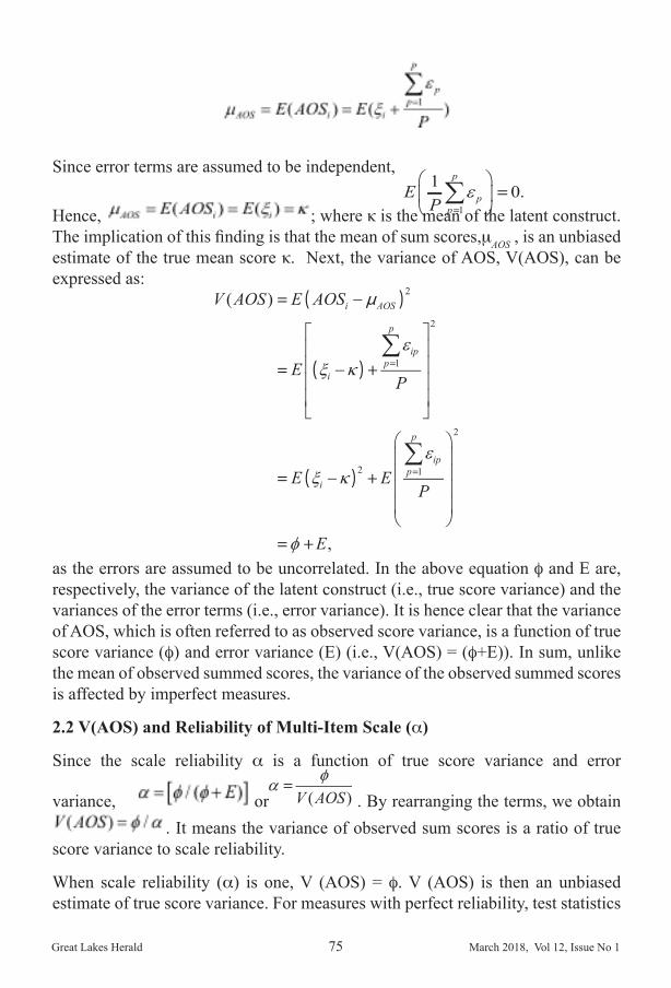
Since error terms are assumed to be independent,

Hence, ; where κ is the mean of the latent construct. The implication of this finding is that the mean of sum scores,μAOS , is an unbiased estimate of the true mean score κ. Next, the variance of AOS, V(AOS), can be expressed as:

as the errors are assumed to be uncorrelated. In the above equation φ and E are, respectively, the variance of the latent construct (i.e., true score variance) and the variances of the error terms (i.e., error variance). It is hence clear that the variance of AOS, which is often referred to as observed score variance, is a function of true score variance (φ) and error variance (E) (i.e., V(AOS) = (φ+E)). In sum, unlike the mean of observed summed scores, the variance of the observed summed scores is affected by imperfect measures.

2.2 V(AOS) and Reliability of Multi-Item Scale (α)

Since the scale reliability α is a function of true score variance and error

variance, or . By rearranging the terms, we obtain . It means the variance of observed sum scores is a ratio of true

score variance to scale reliability.

When scale reliability (α) is one, V (AOS) = φ. V (AOS) is then an unbiased estimate of true score variance. For measures with perfect reliability, test statistics


in ANOVA do not require any correction or disattenuation. But, when the measure is imperfect (i.e., reliability is less than one), V(AOS) will be larger than true score variance. Since V(AOS) appears in the denominator of ANOVA statistics, larger values of V(AOS) attenuate the test statistics. So to correct for this attenuation, V(AOS) must be multiplied by scale reliability α. The correction will ensure that ANOVA based statistics use an estimate of true score variance (φ) instead (i.e.,

replaces V(AOS)). We apply this finding when disattenuating the F-statistic and the associated effect size, f, in ANOVA.

2.3 Disattenuation of F-Statistic

Suppose we have G groups, where AOSig is the sum score for subject i in group g, is the mean of sum scores in group g, is the grand mean, κg is the latent mean of group g, κ is the grand mean of latent scores, ng is the sample size for group g, and αg is the reliability of the scale in group g. If MSB is the between-group mean square and MSWdisatt is the disattenuated within-group mean square, then

Since the expected value of latent mean is not affected by measurement error, when latent means are replaced by their sample estimates, we obtain:

(1)

where is the sample estimate of latent mean for group g based on the analysis of sum scores, and is the sample estimate of the grand or overall mean. Notice that in the above equation, the numerator is the between-group sum of squares (SSB) and the denominator is the degrees of freedom.

The within-group sum of squares is computed as:

Replacing κg , the latent mean for group g, with the sample mean , we get

(2)

Since the variance of AOS is affected by measurement error, and as the


true variance is equal to the sample variance multiplied by scale reliability (i.e., ), the disattenuated sample estimate of within-group sum of squares for group g is given by

where αg is the reliability of group g. Across G groups, the disattenuated pooled within-group sum of squares is then computed as:

(3)

The pooled within-group disattenuated mean square of experimental error (i.e., disattenuated pooled within-group variance, MSW,disatt) is then obtained as follows.

Let V(AOSg ) be the within-group variance of group g, then MSWdisatt can be expressed as:

MSWdisatt = (4)

The disattenuated F-statistic, corrected for attenuation or measurement error, is then computed as follows:

(5)

where αg is the scale reliability of group g.

When the scale reliability is 1.0 for all G groups, Fdisatt in equation (1) would become the F-statistic as reported in an ANOVA. In contrast, for any group g, if the measurement error reduces scale reliability to a value that is less than 1.0, then the denominator of equation (1) (i.e., within-group mean square) becomes smaller, and correspondingly, the F-statistic becomes larger. In that scenario, Fdisatt would serve as the disattenuated (or corrected) version of the F-statistic – one that accounts for measurement error.


The disattenuated F-statistic reveals what the true magnitude of the test statistic is for latent mean differences for error-free measures. Because statistical packages (e.g., SAS and SPSS) do not take into account scale reliability and measurement error when computing the F-statistic, it must be disattenuated prior to testing the significance of latent mean differences. The extent of this disattenuation depends, of course, on the size of the measurement error as reflected in the measure of scale reliability, such as coefficient alpha.

In order to better understand the boundary conditions for reliability, we constructed the chart shown in Figure 1. It shows the degree to which the test statistic F requires correction (or disattenuation) for varying levels of reliability. The figure underscores our argument that while the statistical significance of the F-statistic is known to be a function of sample size, size of group mean differences, and within-group variance in responses; the scale reliability also needs to be taken into account in order to assess the true significance of latent mean differences.

Figure 1: Relationship between Percentage Disattenuation and Reliability


Note:

(1) Figure 1 shows the degree to which test statistics need to be disattenuated for various levels of reliability.

(2) It is assumed that the measure reliability is assumed to be the same for all groups across all values of reliability.

(3) Equations 5 and 8 show how to compute the disattenuated statistics when measure reliability varies across groups.

The correction factor for attenuation is consequently a function of how reliability is measured. Two of the most popular ways of measuring reliability are coefficient alpha and composite reliability. Between them, it is often mentioned in the literature that coefficient alpha represents a lower bound for scale reliability (Guttman, 1945). If that were to be true, then the correction factor will be higher when coefficient alpha is used in place of composite reliability. However, Peterson and Kim (2013) performed an analysis of 2524 pairs of coefficient alpha and composite reliability – values they derived from empirical investigations. They concluded that the difference between the two reliability estimates is inconsequential (average composite reliability was .86 versus the corresponding average coefficient alpha of .84). Estimating composite reliability requires application of SEM, while coefficient alpha can be estimated in an ANOVA setting. As most studies use ANOVA, we can infer from the Peterson and Kim (2013) study that one could use coefficient alpha instead to correct the relevant statistics for attenuation.

2.4 Disattenuation of Effect Size (f)

Cohen (1988) defined the effect size (f) in ANOVA as the standardized value of the standard deviation of mean differences. If σm is the standard deviation of population means and σ is the pooled standard deviation of AOS across g groups, then the standardized effect size can be expressed as:

where

If σ g is the standard deviation of sum scores in the gth group, then the pooled standard deviation can be computed as:


By replacing the population parameters by their corresponding sample estimates, we obtain the effect size estimate for the sample as:

= (6)

Once again, it must be noted that the numerator, which represents the standard deviation of mean differences, is unaffected by measurement error. The denominator, which represents standard deviation of sum score means, is, however, affected by measurement error. Hence, the correction applies to the denominator of the effect size formula. Based on the previous discussion about disattenuating within-group sum of squares, the disattenuated pooled within-group standard deviation can be expressed as:

(7)

where αg is the scale reliability in group g and V(AOSg) is the standard deviation of AOS within group g.

The disattenuated effect size fdisatt can then be obtained by dividing sm by sdisatt as follows:

In equation (8), fdisatt reflects what the true effect size would be, if we were to employ


measures uncontaminated by measurement error. In addition, if the construct is measured with perfect reliability (i.e., αg=1), fdisatt will become the standardized effect size estimate f. Figure 1 shows boundary conditions that capture the relationship between reliability and effect size f. The extent of disattenuation for f can be as high as 29.1% when reliability is .6 – a value that is close to the reliability of measures that some authors reported in previous studies – and approaches 0% when scale reliability is close to 1.

Here we have described how to obtain the disattenuated F-statistic and the associated effect size f. In subsequent sections, we apply the attenuated and disattenuated F-statistics and effect-size estimates to two datasets from the extant OM literature to demonstrate the degree of attenuation in mean difference tests and its consequences.

3. Application of the Disattenuation Procedure in Mean Difference Tests in Decision Sciences

We use two anonymous examples, both drawn from the public domain, to illustrate the proposed disattenuation procedure. The first example will show the impact of disattenuation on the outcome of the overall statistical test and effect size when the overall F statistic is not significant prior to disattenuation. The second example will then describe the impact of disattenuation on the outcome of pairwise mean comparisons. The purpose of using the second example is to illustrate what additional insights can be drawn via disattenuation, even when the overall attenuated F-statistic reveals significant mean differences to begin with. As such, the second example will answer the question as to why it is imperative to disattenuate ANOVA statistics even if the F-statistic was significant prior to disattenuation.

Example 1. Comparing Manufacturing Flexibility Across Firms in Different SIC Groups

Suppose we investigate whether manufacturing flexibility varies across firms that are classified into three different SIC industry groups. For illustration purposes, we focus on four of the flexibility measures that the authors of the original study proposed in a top-tier journal – coded as LFU, NPFRN, NPFM, and MDFRH – and compare their means across firms that are classified into 3 SIC industry groups. All measures are based on multi-item, 7-point rating scales; the number of scale items is 6 for LFU, 5 each for NPFRN and NPFM, and 4 for MDFRH. All four measures have acceptable reliability levels, with reported coefficient alphas above .7. Reliabilities, sample sizes, and results of ANOVA are all presented in Table 1. Computations of disattenuated statistics of ANOVA results are illustrated for the MDFRH measure in Appendix A.


It is worth noting that for highly reliable scales, the degree of attenuation will be small. For such scales, the outcome of the statistical test (i.e., statistical significance) is unlikely to change if the p-value associated with the F-test is also high (e.g., p=0.16 for LFU). For the LFU measure, the F-statistic disattenuates by only about 6.03% and the p-value of disattenuated F decreased only marginally to 0.14. Parenthetically, if the reliability of the LFU measure were to be .7 – a value that is close to the lower end of the acceptance for scale reliability, then the attenuation of the F-statistic would have been as high as 42.86% and the disattenuated p-value would have been closer to 0.07. For measures whose reliability crosses the minimum threshold for acceptance, the relationship between reliability and the percent to which F disattenuates is already shown in Figure 1 as discussed previously. So, for the LFU measure, given its high reliability across the 3 SIC groups, the mean difference remained insignificant with or without disattenuation.

But, even when a measure has high reliability, disattenuation could still change the outcome of the statistical test. In Table 1, results associated with NPFRN serve as an exemplar of this scenario, where disattenuation changes p-value from 0.06 to 0.04, making the mean difference significant, when that was not the case prior to disattenuation procedure being applied. Next, when measures exhibit moderate to high reliabilities (.76 to .85), the outcomes of statistical tests are likely to change when the test statistics are disattenuated, as illustrated by the analysis of NPFU and MFRH measures.

Overall, across the four scales, the F-statistic attenuation ranged from 6.03% to 25.64% and the effect size attenuation ranged from about 3% to as high as 12.09%. This analysis clearly illustrates why the test statistic and effect size need to be disattenuated to account for imperfect measurement scales. So, Example 1 demonstrates that disattenuation is more likely to change the outcome when scale reliabilities are closer to the acceptance threshold (.7 or above). When scale reliabilities are high, then the outcome is likely to change only if the p-value of the attenuated F statistic is closer to the acceptance level. Even when disattenuation is unlikely to change statistical outcome for highly reliable measures, the effect size will still increase. This was indeed the case for LFU when effect size increased by about 3% after disattenuation was applied.


Table 1: Impact of SIC Industry Groups on the Dependent Variables – ANOVA Results

Dependent VariablesLFU NPFRN NPFU MDFRH

N for each SIC group 45, 39. 57 47, 37, 57 47, 35, 56 47 37, 57Number of Scale Items 6 5 5 4MSB (mean square between) 2.75 6.42 2.73 3.14

MSE (mean square error) 1.49 2.29 1.21 1.05Sm (std dev means) 0.20 0.30 0.20 0.21S (pooled within grp std dev) 1.21 1.51 1.10 1.03

Fatt 1.85 2.81 2.26 2.98Fatt,prob 0.16 0.06 0.11 0.054

Reliability for each group 0.97, 0.95, 0.91

0.90, 0.84, 0.93

0.86, 0.76, 0.85

0.77,0.79, 0.82

Fdisatt 1.97 3.10 2.70 3.74Fdisatt,prob 0.14 0.04 0.07 0.03Does disattenuation change outcome of statistical test? No Yes, at .05

levelYes, at .10

levelYes, at .05

level% Disatt F Statistic 6.03% 10.58% 19.57% 25.64%fatt (attenuated effect size) 0.16 0.20 0.18 0.20fdisatt 0.17 0.21 0.20 0.23% Disatt Effect Size 2.98% 5.17% 9.35% 12.09%

Example 2: Adoption of Lean Supply Chain Strategy Across Six Different Company Types

In this example, we use data from a different anonymous study that also appeared in a top-tier journal in the field of Decision Sciences. Here too our focus is to bring out the value of the new methodology that we are proposing in this paper, rather than on confirming or rejecting the results obtained in the original study. For illustration purposes, we focus only on the six-item measure of the dependent variable (adoption of lean supply chain strategy) and whether it is affected by type of ownership of the company. Data were originally collected on the dependent measure from companies that are categorized into six different groups based on type of ownership. For our purposes, the numbers 1 to 6 identifies those six company groups. Attenuated ANOVA results indicate that the mean rating on the dependent variable is significantly different across the six company types (F(5,598)=4.08, p<.01). So, disattenuation would not change the overall outcome of the results


in this case. However, we still apply the disattenuation procedure to explore what other insights could be derived when performing pairwise mean comparisons – which is a logical next step whenever the overall F statistic is significant.

The results of pairwise mean comparisons, based on Tukey’s Studentized range tests, are presented in Table 2. Since the Studentized range statistic (Qatt) is similar to the t-statistic, it too is affected by scale reliability. Qdisatt is the disattenuated version of Qatt. Values of Qdisatt are also provided in Table 2 along with the effect size estimates relevant for pairwise comparisons (Cohen’s datt and ddisatt). For illustration purposes, we selected two groups of firms which exhibited significant mean differences (with respect to adoption of lean supplier chain strategy) prior to disattenuation and three other groups of firms whose means did not differ significantly at first. Without disattenuation, only the mean of group 2 firms is significantly different from the mean of group 4 firms. But, if we were to apply the disattenuated Studentized range statistic (Qdisatt), we would find other significant mean differences -- between groups 1 versus 4 (p=0.02), and 2 versus 3 (p=0.02). The mean difference between group 4 and group 6 approaches significance, but the p-value (.054) is still above .05. The effect size estimates for these group mean differences are not small, ranging from .44 to .47 based on disattenuated Cohen’s d statistic. Such significant pairwise mean differences and the fairly moderate effect sizes associated with those mean differences could be easily overlooked if DS researchers were to ignore disattenuation in those cases where the attenuated F-statistic initially reveals significant mean differences.


Table 2: Adoption of Lean Supply Chain Strategy Across Company Types: Results of Selected Pairwise Mean Comparisons

StatisticCompany Type

(2) Versus (4) (1) Versus (4) (4) Versus (6) (2) Versus (3)Mean dif 0.56* 0.34** 0.31 0.35**Qatt 6.42 3.90 3.55 4.01

Qatt prob 0.00 0.07 0.12 0.05

Qdisatt 7.22 4.39 4.00 4.51

Qdisatt prob 0.00 0.02 0.05 0.02

Cohen datt 0.66 0.43 0.39 0.42

Cohen ddisatt 0.74 0.49 0.44 0.47

Outcome of disattenuation

No change, mean difference was significant before disattenuation

Mean diff became significant after disattenuation

No difference, but approaches significance after disattenuation

Mean difference became significant after disattenuation

Notes:

Results are based on Tukey’s Studentized range statistic Q for pairwise mean difference tests. Q is computed by using the harmonic mean (nh) of the sample sizes for different groups. For the X variable nh is 87.859 and for the Y variable it is 57.432. The Q statistic is obtained as Q = where MSE is the mean square error (= 0.668 for X variable analysis and 0.648 for Y variable analysis. It can be obtained from standard errors and sample sizes of individual groups as reported in the anonymous study.

Qdisatt statistic is computed as where α is scale reliability (=.79)

The various X groups are described in the anonymous study.

Only mean differences marked by ‘*’ are reported as significant in the anonymous study. Mean differences marked by ‘**’ are also significant (p<.05) based on Qdisatt

For pairwise mean differences, Cohen’s d and Cohen’s dd reflect effect size estimates (attenuated and disattenuated). Assuming n1 and n2 are sample sizes of

(X1)-(X2)√(MSE/n h)


groups 1 and 2, Cohen’s ddisatt is computed as:

In sum, the two examples show that when ANOVA studies use attenuated statistics instead of disattenuated statistics, researchers may draw incorrect inferences as they relate to overall significance or pairwise mean differences. The likelihood of drawing incorrect inferences is dependent on measure reliability and its impact on attenuation of test statistics. Based on equations (5) (for the F-statistic) and (8) (for effect size f), the degree of attenuation is solely a function of scale reliability. Neither the sample size nor size of mean differences has any impact.

4. Discussion

Hypothesizing and testing for between-group mean differences of latent constructs is critical to theory testing in DS research. But, application of ANOVA in this regard leads to attenuation of the F statistic when the measures are imperfect (i.e., reliability is less than one). Our study shows how to correct the F-statistic and the associated effect size f for this attenuation. For DS researchers, the procedure outlined in this paper can be a viable alternative to SEM when they are compelled to use ANOVA for a variety of reasons, such as when they are faced with small samples, when the latent constructs are measured by a large number of scale items, and/or when the maximum likelihood procedure in SEM fails to converge. These conditions are often encountered in many practical settings within which DS research is conducted. Further, in ANOVA, the disattenuated statistics are easier to obtain, as the correction for attenuation applies only to the within-group sum of squares. No correction is necessary for the between-group sum of squares, whether it is for the main or interaction effects.

The advantages of using our proposed procedure presented in this study are a) once adopted, it would ensure that DS empirical research, moving forward, conducts latent mean difference tests correctly when using ANOVA, b) it offers authors of existing research an opportunity to ascertain the accuracy of their previously-reported results and conclusions, and c) it allows researchers who had sound measures (i.e., acceptable reliability), but who did not submit their work for review because of the perceived “editorial bias against the null” (Hubbard & Armstrong, 1997), to reevaluate their work to see if applying our procedure would make a difference to their study findings. Accurate effect size estimation is important, even in cases where the attenuated ANOVA statistics show significant mean differences. As such, the suggested procedure is applicable to all researchers


in DS who work with imperfect multi-item measures, and whose objective is to examine between-group mean differences.

The proposed disattenuation procedure will change the outcome (statistical significance) in some, but not all cases, while increasing effect sizes across the board – a key point to consider, given the renewed call in social sciences to only use effect size as the basis for interpreting between-group mean differences (Kline, 2013). Kline (2013) has argued that the effect size is more important than the test statistic, and that researchers should discount test statistics altogether because decisions based on test statistics may not be correct due to Type I and Type II errors, and the best way to advance theory is via replication. As per Hubbard and Armstrong (1997) and Kline (2013), our focus in should be on effect size rather than on statistical significance per se. This argument is meritorious given that meta-analysis studies have shown that conclusions based on statistical-significance tests have been wrong (Rossi, 1997).

5. Conclusion

Our disattenuation procedure is not meant to be used as a tool to make insignificant results become significant. We do not advocate using poor quality measures whose reliabilities are below the values recommended in published research (cf. Nunnally, 1978). Rather, if the measures are based on sound theory and possess acceptable but imperfect reliabilities (i.e., α<1), then our approach would help determine whether the true score mean differences would be significant, and what the true effect size would be -- one that can be compared across studies. As studies based on measures with imperfect reliability continue to receive journal space, our approach will help those studies report the true effect size estimates when corrected for reliability. Within this context, future research should examine how the disattenuation procedure presented in this paper compares with contemporary techniques like HLM when accounting for measurement error.

Overall, the intent of our paper is not to take a position on this debate of whether or not statistical tests in Decision Sciences research should be used exclusively or in conjunction with effect-size estimates. Our objective, instead, has been to demonstrate that ANOVA-based statistics should be disattenuated, and to offer the ANOVA framework as a viable alternative to SEM even when the underlying measures have imperfect reliability, so long as the F and f statistics are first disattenuated. Following this approach will improve the quality of findings in future DS research, allow more definitive effects to be identified, and make the conclusions more meaningful and valid.


REFERENCES

Bobko, P., Roth, P.L., & Bobko, C. (2001). Correcting the effect size of d for range restriction and unreliability. Organizational Research Methods, 4 (1), 46-61.

Bendoly, E., Rosenzweig, E., & Stratman. J. (2009). The efficient use of enterprise information for strategic advantage: a DEA analysis. Journal of Operations Management. 27(4), 310-323.

Buell, R.W., & Norton, M.I. (2011). The labor illusion: How operational transparency increases perceived value. Management Science, 57 (9), 1564-1579.

Cohen, J. 1988. Statistical Power Analysis for the Behavioral Sciences (2nd ed.). Hillsdale, NJ: Lawrence Erlbaum Associates.

de Guinea, A.O., & Webster, J. (2013). An investigation of information systems use patterns: technological events as triggers, the effect of time, and consequences for performance. MIS Quarterly, 37 (4), 1165-A6.

Durvasula, S., Sharma, S., & Carter, K. (2012). Correcting the t statistic for measurement error. Marketing Letters, 23, 671-682.

Forza, C. (2002). Survey research in operations management: A process-based perspective. International Journal of Operations & Production Management, 22 (2), 152-194.

Guttman, L. (1945). A basis for analyzing test-retest reliability. Psychometrika, 10, 255–282.

Hekman, D.R., Johnson, S.K., Foo, M., & Yang, W. (2017). Does diversity-valuing behavior result in diminished performance ratings for non-white and female leaders? Academy of Management Journal, 60 (2), 771-197.

Hubbard, R., & Armstrong, J.S. (1997). Publication bias against null results. Psychological Reports, 80, 337-338.

Kim, E., Bhave, D. & Glomb. TM. (2013), Emotion regulation in workgroups: The roles of demographic diversity and relational work context. Personnel Psychology, 66, 613-644.

Kline, Rex B. 2013. Reforming Data Analysis Methods in Behavioral Sciences, Washington, D.C.: American Psychological Association.

Kopalle, P.K, Lehmann, D.R., & Farley, J.U. (2010). Consumer expectations and culture: The effect of belief in karma in India. Journal of Consumer Research, 37 (August), 251-263.


Koufteros, X., Droge, C., Heim, G., Massad, N., & Vickery, S.K. (2014). Encounter satisfaction in e-tailing: Are the relationships of order fulfillment service quality with its antecedents and consequences moderated by historical satisfaction? Decision Sciences, 45(1): 5-48.

Malhotra, M.K., & Grover, V. (1998). An assessment of survey research in POM: From Constructs to theory. Journal of Operations Management, 16 (4), 407-425.

Martin, S.R. (2016). Stories about values and valuable stories: A field experiment of the power of narratives to shape newcomers’ actions. Academy of Management Journal, 59 (5), 1707-1724.

Nunnally, J.C. (1978). Psychometric Theory (2nd ed.). New York: McGraw-Hill.

Nunnally, J.C., & Bernstein, I.H. (1994). Psychometric Theory (3rd ed.). New York: McGraw-Hill.

Peterson, R.A. & Kim, Y. (2013). On the relationship between coefficient alpha and composite reliability. Journal of Applied Psychology, 98 (1), 194-198.

Rossi, J.S. (1997). A case study in the failure of psychology as a cumulative science: The spontaneoous recovery of verbal learning. In L.L. Harlow, Mullaik, S.A., & Steiger, J.H. (Eds.), What if there were no significance rests? Mahwah, NJ: Lawrence Erlbaum Associates, 175-197.

Saeed, K., A. Malhotra, M., K., & Grover, V. (2011). Inter-Organizational System Characteristics and Supply Chain Integration: An Empirical Assessment, Decision Sciences, 42(1), 7-40.

Schoenherr, T., Power, D., Narasimhan, R., & Samson, D. (2012). Competitive capabilities among manufacturing plants in developing, emerging, and industrialized countries: A comparative analysis. Decision Sciences, 43 (1), 37-71.

Verma, R., & Goodale, J.C. (1995). Statistical power in operations management research. Journal of Operations Management, 13(2), 139-152.


Appendix A: Computations of Disattenuated Statistics of Anova Results for The MDFRH Measure

Industry 1

Industry 2

Industry 3 MSB MSW F(2, 138) F prob

Sample Size 47 37 57 3.14 1.05 3.14 0.05

Mean ( ) 3.25 2.87 3.39

Grand Mean 3.21

Variance1.16 1.00 01.00

Reliability (g) 0.77 0.79 0.82

Computing Fdisatt

From equation 4 MSWdisattenuated is computed as:

Fdisatt = = ; Fdisatt prob = 0.026

Computing effect size fdisatt

From equation 6, (standard deviation of means) =

From the equation 7, disattenuated Pooled within-group variance


From equation 8, Disattenuated effect size (fdisatt) = / = 0.21/0.92 = 0.23

A Simple Procedure to Correct for Attenuation of ANOVA ...

Documents

Transcript of A Simple Procedure to Correct for Attenuation of ANOVA ...