This document is downloaded from DR‑NTU (https://dr.ntu.edu.sg)Nanyang Technological University, Singapore.

A simple model for predicting the pressure dropand film thickness of non‑Newtonian annularflows in horizontal pipes

Li, Haiwang; Wong, Teck Neng; Skote, Martin; Duan, Fei

2013

Li, H., Wong, T. N., Skote, M., & Duan, F. (2013). A simple model for predicting the pressuredrop and film thickness of non‑Newtonian annular flows in horizontal pipes. ChemicalEngineering Science, 102,121‑128.

https://hdl.handle.net/10356/106838

https://doi.org/10.1016/j.ces.2013.07.046

© 2013 Elsevier Ltd. This is the author created version of a work that has been peerreviewed and accepted for publication by Chemical Engineering Science, Elsevier Ltd. Itincorporates referee’s comments but changes resulting from the publishing process, suchas copyediting, structural formatting, may not be reflected in this document. The publishedversion is available at: [http://dx.doi.org/10.1016/j.ces.2013.07.046].

Downloaded on 06 Dec 2021 14:13:54 SGT

Author's Accepted Manuscript

A simple model for predicting the pressuredrop and film thickness of non-Newtonianannular flows in horizontal pipes

Haiwang Li, Teck Neng Wong, Martin Skote, FeiDuan

PII: S0009-2509(13)00539-3DOI: http://dx.doi.org/10.1016/j.ces.2013.07.046Reference: CES11216

To appear in: Chemical Engineering Science

Received date: 19 March 2013Revised date: 7 June 2013Accepted date: 28 July 2013

Cite this article as: Haiwang Li, Teck Neng Wong, Martin Skote, Fei Duan, Asimple model for predicting the pressure drop and film thickness of non-Newtonian annular flows in horizontal pipes, Chemical Engineering Science, http://dx.doi.org/10.1016/j.ces.2013.07.046

This is a PDF file of an unedited manuscript that has been accepted forpublication. As a service to our customers we are providing this early version ofthe manuscript. The manuscript will undergo copyediting, typesetting, andreview of the resulting galley proof before it is published in its final citable form.Please note that during the production process errors may be discovered whichcould affect the content, and all legal disclaimers that apply to the journalpertain.

www.elsevier.com/locate/ces

1

A simple model for predicting the pressure drop and film thickness of non-Newtonian 1annular flows in horizontal pipes 2

3 Haiwang Li1,2, Teck Neng Wong1,*, Martin Skote1, Fei Duan14

51School of Mechanical and Aerospace Engineering, Nanyang Technological University 6

50 Nanyang, Avenue, Singapore 639798, 72National Key Lab. of Science and Technology on Aero-Engines, Beijing University of 8

Aeronautics and Astronautics, 9Beijing, 100191, China 10

*Corresponding author. E-mail: mtnwong@ntu.edu.sg 1112

Abstract13

A model of two-phase non-Newtonian horizontal annular flows, which predicts film 14

thickness and pressure gradient from flowrates only, is presented. In the model, the gas and 15

non-Newtonian liquid flows are calculated separately based on the independent governing 16

equations. The shear stress balance at the gas-liquid interface is calculated in order to link 17

two phases together. The non-Newtonian fluid is assumed as a power-law shear-thinning 18

liquid. The logarithmic velocity distribution is chosen to calculate the turbulent velocity 19

profile in the gas core. The influences of entrainment and aeration are included in the model. 20

The pressure drop, film thickness, void fraction, the frictional multiplier, and 21

Lockhart-Martinelli parameter are predicted. The analytical model is compared with the 22

published experimental investigations, and the results show that the model can predict the 23

film thickness and pressure gradient simultaneously based on the flowrates of liquid and gas. 24

The frictional multiplier and Lockhart-Martinelli parameter are calculated at the same time, 25

and the predicted values are comparable with the experimental data. The difference between 26

the analytical model and the experiments is lower than 10%. 27

28

Keywords: Fluid Mechanics, Mathematical modeling, Multiphase flow, Non-Newtonian 29

fluids, Annular, entrainment 30

Introduction 31

In the recent years, considerable effort has been made to study simultaneous gas-liquid 32

2

flows in horizontal and inclined pipes (Al-Kizwini et al., 2013; Okawa et al., 2010; Tai and 1

Chung, 2010; Wang et al., 2012). The two-phase flows are commonly found in power plants, 2

chemical processes, nuclear reactors, and petroleum related industries. The three most 3

important hydrodynamic features of gas-liquid flows in engineering applications, including 4

the flow pattern, the void fraction, and the pressure drop of two-phase flows, have been 5

studied experimentally and theoretically (Al-Kizwini et al., 2013; Al-Sarkhi et al., 2012; 6

Baniamerian et al., 2012; Cioncolini and Thome, 2012; Okawa et al., 2010; Ren et al., 2012; 7

Tai and Chung, 2010; Wang et al., 2012; Xiao et al., 2011). An annular flow, which occurs at 8

relatively high gas flowrates, is defined with a gas core in the center of the channel and an 9

annular liquid film adjacent to the channel wall. With wide applications can be found in the 10

process industries (Srivastava, 1977), the annular flow has been investigated experimentally 11

(Al-Kizwini et al., 2013; Ashwood, 2010; Brill and Begss, 1978; G. F. Hewitt, 1969; 12

Lockhart and Martinelli, 1949; Ren et al., 2012) and numerically (Rodriguez, 2009; Tai and 13

Chung, 2010). 14

Prediction of pressure loss and void fraction of annular flow is important for the accurate 15

design and optimization of multi-phase flows systems, as evidenced by the engineering 16

model development in decades (Ashwood, 2010; Cioncolini and Thome, 2012; Xiao et al., 17

2011). The annular flow is traditionally analyzed through the triangular relationship (G. F. 18

Hewitt, 1969). Modeling of the annular flow can be generally broken into two physical 19

concepts. The first model, derived by the Ref (Owen and Hewitt, 1987), is a single-zone one 20

which describes the film without distinction between the wall and free waved interface. As 21

originally presented, this model yields an estimate average film thickness and pressure loss 22

according to the entrainment data. Hurlburt and co-worker (Hurlburt, 2006; Schubring, 2009; 23

Wallis, 1969) developed another model, in which the waves and the base film were modeled 24

separately. Following the concept of Hurlburt, the effect of entrained fraction is added to 25

compute the local interfacial shear. The effects of base-wave division, coupling film and 26

entrainment behavior were considered in the model of Hurlburt (Hurlburt, 2006). Schubring 27

and co-worker (Schubring and Shedd, 2008, 2009a, b, 2011) developed the models which 28

3

include effects of wave magnitude, wave intermittency, and the sharp transitions between 1

base film and disturbance waves. However, the previous research efforts have been heavily 2

directed toward the two-phase flow of gas and Newtonian liquid, despite the increasing 3

industrial importance of non-Newtonian liquids, such as aeration of Newtonian broths in 4

biochemical reactors, continuous polymerization, transport of such non-Newtonian liquid 5

materials as drilling mud, greases, slurries, polymer solutions, etc. Limited information is 6

available for the case when the liquid phase is non-Newtonian flow. Therefore, it needs to 7

understand the annular flow behavior of non-Newtonian two-phase flow. 8

As an annular flow is often understood through triangular relationship, the empirical 9

relationship among film thickness, pressure drop, and flowrates (Srivastava and 10

Narasimhamurty, 1973; Tyagi and Srivastava, 1976; Xu et al., 2007) has been previously 11

analyzed. Srivastava and his co-worker (Srivastava, 1977; Tyagi and Srivastava, 1976) 12

proposed a non-Newtonian liquid-gas annular flow model to predict liquid holdup and 13

two-phase pressure drop. The logarithmic velocity distribution of turbulent flow was used to 14

predict the velocity distribution of the gas core. The previous work (Eisenberg and 15

Weinberger, 1979) measured the pressure drop and void fraction of two-phase 16

non-Newtonian flows; the measured results were compared with the model prediction which 17

was a modified version of the two-phase Newtonian flow. As a PhD student, Shu extended 18

the Newtonian model to the non-Newtonian two-phase flow model based on the relationship 19

of properties between Newtonian and non-Newtonian fluids (Shu, 1981). These models are 20

developed using the concept of triangular relationship of the annular flow. In order to 21

calculate one parameter, i.e. film thickness, the other parameters of flowrates and pressure 22

drop should be known. The application of models are limited because the values of film 23

thickness and pressure drop of a two-phase flow are difficult to be measured (Ashwood, 24

2010).25

In summary, most of the previous modeling works have focused on the Newtonian flow, 26

and either pressure gradient or film thickness needs to be known although they are very 27

difficult to measure. In addition, the effects of aeration and entrainment were ignored in most 28

4

of studies. The model presented here improves these deficiencies. This paper develops a 1

model to predict the pressure drop and film thickness of a two-phase non-Newtonian 2

horizontal annular flow; the effects of entrainment and aeration are taken into account into 3

the model. The pressure drop, film thickness, void fraction, the frictional multiplier, and 4

Lockhart-Martinelli parameter are obtained using this model. These analytical results are 5

compared with the published experimental data (Schubring and Shedd, 2009a; Shu, 1981). 6

The paper is organized as follows: in section 2, the mathematical model is derived based 7

on the assumption of the logarithmic velocity distribution in the gas core. The results and 8

discussion are presented in section 3. The relationship among the void fraction, the frictional 9

multiplier, and Lockhart-Martinelli parameter are presented. The conclusions from the model 10

are presented in section 4. 11

122. Mathematical model 13

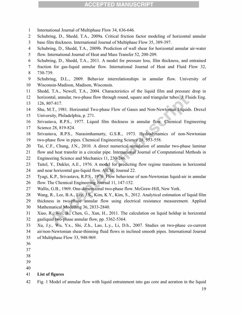
Figure 1 shows the model of a two-phase annular flow including the effects of 14

entrainment and aeration. In the annular flow, there exists an interface between the liquid film 15

and the gas core. In practice this vapor-liquid interface is covered by a complex pattern of 16

waves. The liquid in the form of small droplets, and the gas as small bubbles, are entrained 17

into the gas core and the liquid film, respectively, through the interfaces. However, for the 18

theoretical analysis, a model of the flow conditions is conceived and shown in Fig. 1 with the 19

following assumptions (Eisenberg and Weinberger, 1979; Shedd and Newell, 2004; Shu, 1981; 20

Srivastava, 1977): 21

(1) The flow in liquid film is laminar while the flow in gas core is turbulent. 22

(2) The liquid film is assumed symmetrical. 23

(3) The liquid film and the gas core have the same pressure gradient along flow 24

direction. 25

(4) Zero pressure gradients exist in the radial direction. 26

(5) The gas velocity is the sum of the interfacial velocity and the turbulent component. 27

(6) The interface between the liquid film and gas core is smooth. 28

(7) There is no velocity slip either between liquid and the tube wall or between liquid 29

5

and gas. 1

(8) The gravitational and acceleration efforts can be ignored in the both liquid and gas 2

phases. 3

(9) Densities of gas and non-Newtonian liquid are constant. 4

This model proceeds through the following steps: 5

(i) The flowrate of liquid film and gas core are obtained firstly; 6

(ii) The film thickness is estimated under the constant flowrates of gas and liquid; 7

(iii) The pressure drop in the two-phase flow is calculated according to the flowrates 8

and film thickness; 9

(iv) The single-phase pressure drop is established; 10

(v) The multiplier ( L� ) and Lockhart-Martinelli parameter (X) are established 11

according to single-phase and two-phase pressure drop. 12

13

2.1. Governing equation of liquid film 14

The momentum equation in the cylindrical coordinates can be described as (G. F. Hewitt, 15

1969; Shu, 1981) 16

� �1 0rzP rz r r

�� �� � � �

(1) 17

where r and z are the radial and axial directions of cylindrical coordinates, and � is the 18

average value of shear stress. This equation is also the force balance of liquid and gas. The 19

first term is the pressure gradient, and the second term is the shear stress. In Eq.(1), the 20

viscous stress � can be described as 21

numr

� � � �� �� (2) 22

for the power-law model. In the two-phase flow, m is called flow consistency index and n is 23

denoted as flow behavior index. The fluid is shear thinning for 1n � , and shear thickening 24

flow for 1n � . Noted that a Newtonian liquid can be considered to be a power-law liquid 25

with an exponent n = 1. The viscosity of liquid film can be described as (Wallis, 1969) 26

6

(1 )f f G f L� � � � � � � (3) 1

where f� is the viscosity of liquid film, f� is the fraction of aeration in liquid film, G�2

is the viscosity of pure gas, and L� is the viscosity of pure liquid. In general case, G� is 3

small compared to the liquid viscosity L� , G L� ��� , and hence Eq. (3) reduces to 4

(1 )f f L� � � � . Therefore, Eq. (1) can be formulated as: 5

1 (1 ) 0n

ft

dP ur mdz r r r�

� �� �� � �� � � � � � � � � � � �� � � �� �

(4) 6

Equation (4) describes the relationship between the pressure gradient and velocity profile. In 7

this equation, the subscript of t� means two-phase. From Eq. (4), the velocity profile of 8

liquid film can be derived as: 9

1 1 11 112(1 ) 1

n

n

tf

dPu A r Bm dz

n��

�

�� � � � �� � � � � � � �� � � � �� � �� � � ! �

� �

(5) 10

where A and B are real number introduced by integration, defined according to the boundary 11

conditions. 12

13

2. 2 Boundary conditions of liquid film 14

The no-slip boundary condition at the wall is used 15

0 at f tu r R (6) 16

where tR is the radius of the tube. The other boundary condition is the velocity at the 17

interface ir R , where iR is the radius of the interface. From the force balance at the 18

interface, the relationship between shear stress and pressure gradient can be described as 19

22rz i it

dPR Rdz �

� " " �� � �� � �

(7) 20

where the subscript of r and z indicated r and z direction, and the shear stress rz� can be 21

written as 22

7

=(1 )n

frz f

um

r� �

� �� �� �� �

(8) 1

According to Eqs. (7) and (8), the boundary condition for the velocity at the interface can be 2

expressed as 31

(1 ) 12(1 )

n

n nf i

tf

dPu C Rm dz ��

� � � � � � �� � � � � �� �

(9) 4

where C is the real number due to integration. 5

67

2. 3 Velocity profile of liquid film 8

Substituting the boundary conditions described by Eqs. (6) and (9) into Eq. (5), the 9

velocity of liquid film can be written as 101

1 112 (1 ) 1

n nnn n

f ttf

dP nu R rm dz n��

� � � � � � � � � �� � � � � �� � � �� � (10) 11

12

2. 4 Velocity profile of gas core 13

The universal velocity profile is given in the form of three expressions for three regions; 14

the viscous sub-layer, the buffer layer and the inertial layer. These three sections can be found 15

in the previous study (Srivastava, 1977). The velocity distribution in the inertial layer of 16

single-phase flow can be described by a logarithmic profile as (Tyagi and Srivastava, 1976) : 17

2.5ln 5.5turu ruu

�

� # � �� � �

(11) 18

where turu is the velocity of turbulent component along z direction, u� is the friction 19

velocity, and # is the kinematic viscosity of the gas core. The velocity of gas core in a 20

two-phase flow can be divided into two parts (Srivastava, 1977; Tyagi and Srivastava, 1976) 21

i turu u u � (12) 22

where iu is the velocity of interface which can be calculated according Eq. (10). Following 23

the previous work, the friction velocity of u� is defined as i cu� � $ where i� is the 24

8

interfacial shear stress and c$ is the density of the gas core. The interfacial shear stress is 1

defined as (Taitel and Dukler, 1976) 2

� �2

2c c i

i i

u uf

$�

� � � (13) 3

where if is the friction factor of interface, and cu is the average velocity of the gas core. 4

Because of c iu u�� and i cf f (Gazley, 1949) ( cf is the friction factor of gas core at the 5

wall), Eq. (13) can be simplified into 6

2

2c c

i cuf $� � (14) 7

In Eq. (14), cf can be calculated using the suggested method of Taitel and Dukler (Taitel 8

and Dukler, 1976): 9

a

c cc c

c

D uf C#

� �

�� � �

(15) 10

where the subscript of c means gas core, cC is a coefficient (Taitel and Dukler, 1976) with a 11

value of 0.046 for the turbulent flow. cD is the hydraulic diameter, a is an index which is 12

0.2a in the turbulent flow, and c# is the kinematic viscosity of the gas core. The 13

previous work (Agrawal et al., 1973) suggested that cD can be calculated with the following 14

expression 15

4 2cc i

c

AD RS

(16) 16

where cA is the cross-sectional area of gas core and cS is the perimeter of gas core. In Eq. 17

(15), the kinematic viscosity can be described as 18

cc

c

�#$

(17) 19

where c� is the dynamic viscosity of gas core and c$ is the density of gas core. From 20

9

Landel’s work (Landel, 1963), the viscosity of the non-Newtonian gas core can be expressed 1

with 2

� � 2.51c G q� � � � � (18) 3

where G� is the dynamic viscosity and q is the volume fraction of liquid entrained into the 4

gas core. The density of the gas core is related to the flowrates of gas and fluid through: 5

� �1c G Lq q$ $ $ � � � (19) 6

The subscript of G and L refer to gas and liquid respectively. Combining Eqs. (17), (18) and 7

(19), yields the kinematic viscosity of gas core: 8

� �� �

2.511

Gc

G L

qq q

�#

$ $

�� �

� � � (20) 9

The relationship between gas flowrate GQ and gas core flowrate cQ is 10

� �� �11

fc GQ Q

q��

��

(21) 11

The average velocity of gas core is defined according to Eq. (21) 12

� �� � 2

11

f Gc

i

Quq R�

"�

��

(22) 13

Substituting Eqs. (15), (20) and (22) into Eq. (14), the interfacial shear stress can be 14

described as 15

� �� �

� � � �� �

2

41 1121 2 1

a

f fG L aG Gi c i

c

q qQ QC Rq q� �$ $

�# " "

�

� � � �� �� � �� �� �� � � � � � � �� �� � �� �� � � �

(23) 16

From Eq. (23), the friction velocity can be described as 17

� �� �

� �� �

12 2

42

1 121 1

2

a

f fG Gc a

c

i

Q QCq q

u R�

� �# " "

�

�

� � � � �� �� �� � � � �� �� � �� �� �� �� � � � �� �

� �� �� � !

(24) 18

Substituting Eqs. (10) and (11) into Eq. (12), the turbulent component of gas core can be 19

10

calculated with the following expression 11

1 11 2.5 ln 5.52 (1 ) 1

n nnn n

c t itf c

rudP nu R R u um dz n

�� �

�� #

� �� � � �� �� � � � � � � � �� � � � � �� �� �� � � �� � ! (25) 2

3

2.5 Pressure drop 4

Pressure drop can be calculated from the relationship between the flowrate of liquid film 5

and velocity profile. From Eq. (10), the velocity can be obtained and then inserted into the 6

expression: 7

2t

i

R

fR

Q urdr" % (26) 8

where fQ is the volumetric flowrate of the liquid film. Substituting the velocity profile of 9

the liquid film in Eq. (10) into Eq. (26), the flowrate fQ is presented as follows 10

13 1 3 11 2 212

2 (1 ) 1 2 3 1

n nnnn nt in

f t t itf

R RdP n nQ R R Rm dz n n�

"�

� � � ��� � � � � �

� �� �� � ��� � � �� � � � � � � � � � � �� �� � � �� � � �� � �� � � �� � � �� �� � ! � � ! (27) 11

The flowrate of liquid film can be calculated according to the flowrate of the liquid. The 12

relationship is shown as 13

� � � �1 1f f LQ Q q�� � � � (28) 14

where LQ is the total volumetric flowrate of the liquid. From Eqs. (27) and (28), the 15

pressure drop can be calculated according to the volumetric flowrate of the liquid 16

� �� � 3

12 1(1 )1

n

Lf

t t tf

q QdP nm Fdz R n R�

�"�

� �� ��� �� �� � � � � � � � �� �� � � �� � � �� � ! (29) 17

where F can be calculated as: 181

3 1221 1

3 1

nn

i i

t t

R RnFR n R

�� �

� � �

� �� � � �� � � � � � � � �� �� � � � ��� �� � � �� �� �� � !

(30) 19

20

11

2. 6 The value of iR1

The value of iR is the critical parameter of the two-phase flow. The pressure and 2

velocity can be calculated if the value of iR is known. The gas core flowrate cQ can be 3

calculated from the velocity profile (Eq. (25)) 4

0

2iR

c cQ u rdr" % (31) 5

From Eq.(21), the gas flowrate can be calculated as 6

� �� �

1

22

2

1 3 12

3

1.25ln 2.125

12 1 (1 )1

n

aa

iG i

nn n

L n nf i t i

t tft

BRQ H R

q QnI m F R R RR n R

�

#

�"�

�

� �

� � �� �� � � �� �� � � �� �� �

� �� � �� ��� �� �� � � � � � � � � � � � �� � � � � �� � � � �� � !� �

(32) 7

where 8

� �� �

� �� �

12 21 12

1 1

2

a

f fG Gc

c

Q QCq q

B

� �# " "

�� � � � �� �� �� � � � �� �� � �� �� �� �� � � � � �

� �� �� � !

(33) 9

� �� �

� �� �

� �� �

12 21 12

1 112

21

a

f fG Gc

c

f

Q QCq qq

H

� �# " "

"�

�� � � � �� �� �� � � � �� �� � �� �� �� � �� � � � � � � �

� � �� �� � !

(34) 10

� �� �

1

1 12 (1 ) 11

n

ff

q nIm n

"��

� �� � � � �� �� �� � � ! (35) 11

Eq. (32) constitutes the relationship bewtween GQ , LQ and iR . When the value of GQ12

and LQ are known, the value of iR can be calculated. 13

12

1

2.7 Frictional multiplier, L�2

The liquid phase frictional multiplier L� is defined as follows (Lockhart and Martinelli, 3

1949)412

tL

spL

dPdzdPdz

��

� �� ��� �� �� �� � � �� �� ��� �� �� � !

(36) 5

For the single-phase flow of a power-law liquid, 0f� , 0iR , 0q , Eq. (29) 6

reduces into 7

3

2 3 1n

L

spL t t

QdP nmdz R n R"

� � ��� �� �� � � � �� �� � �� � � �� � ! (37) 8

where the subscript of “ spL ” means single-phase liquid. When substituting Eqs. (29) and (37) 9

into Eq. (36), the multiplier can be expressed as 10

� �� �

3 1 22 221 222

1 1 2(1 ) 1 13 1 3 11

nn nn

ni i

L ft tf

q R Rn nn R n R

� ��

�� �

� � �

� �� �� �� � �� � � � � � � � � � � � � � �� � � �� � � � � �� �� � � � �� � � � � �� �� � � �� � !

(38) 11

12

2.8 The Lockhart-Martinelli parameter, X 13

The Lockhart-Martinelli parameter X can be defined as (Lockhart and Martinelli, 1949) 1412

X spL

spG

dPdzdPdz

� �� ��� �� �� �� � � �� �� ��� �� �� � !

(39) 15

This relationship is suitable for two-phase gas / Newtonian flow. For non-Newtonian flow, 16

some researchers (Eisenberg and Weinberger, 1979) defined a modified Lockhart-Martinelli 17

parameter X18

13

1mod 2

modX spL

spG

dPdzdPdz

� �� ��� �� �� �� � � �� �� ��� �� �� � !

(40) 1

with 2

modwall t

spL spLwall spL

dP dPdz dz

�&&

�

�

� � � �� � �� � � �� � � � (41) 3

where wall t�& � and wall spL& � are the average apparent viscosity of the non-Newtonian liquid 4

(Eisenberg and Weinberger, 1979) in the case of annular flow and single-phase flow 5

respectively. The ratio between the two average apparent viscosities is: 6

� � � �

1

3 12

123 1 1 1

3 1

n

wall tn

wall spL n

nnnn

�&& � �

�

�

��

� �� ��� � � �

� � �� �� � � � �� � �� ��� �� � !

(42) 7

with 8

� �2 2

2 2(1 ) 1 1i if

t t

R RqR R

� � �

� � � �� � �

(43) 9

where � is the total void fraction of the two-phase flow. The single-phase gas pressure can 10

be calculated based on the force balance 11

22 t c tspG

dPR Rdz

" � " � � �� � �

(44) 12

From the expression of the shear stress of gas core in Eq.(23), the pressure drop of 13

single-phase gas is 14

2 5

2

2aa

c G G t G G

spG G

C Q R QdPdz

$ $" � "

�� �� �� � �� � �� � � � (45) 15

Substituting Eqs. (41), (42) and Eq. (45) into the definition of X, the modified 16

Lockhart-Martinelli parameter X can be described as 17

14

� �

12

1422 2

233 1

2

2 1 3 1 2 23 1 1 (1

3 1

n

n aa

L G Gtn

G c G t Gn

m n n Q QX RQ C n Rnn

n

" $$ " � "

� �

�

�

�

� �� � � � � � �� �� � � � � � � � � � �� � � � � � �

� � � � � �� � � � � �� � !� � � � �� �� � ��� �� � !

(46) 1

The holdup of liquid, EL, can be calculated as 2

� � � �2 2 2

2

1t i f iL

t

R R R qE

R" � "

"� � � � �

(47) 3

4

3. Results and Discussion 5

The mathematical model for the non-Newtonian fluid flow is compared with the 6

published data from various sources (Ashwood, 2010; Brill and Begss, 1978; Lockhart and 7

Martinelli, 1949; Schubring and Shedd, 2009a; Taitel and Dukler, 1976). However, in the 8

reported data, the volume fraction of liquid entrained and fraction of aeration in liquid film 9

are unknown. Hence, in the present study, when the analytical model is compared with 10

experimental data, the volume fraction of liquid entrained and the fraction of aeration of 11

liquid film are set as zero. The analytical results are presented regarding the pressure drop of 12

two-phase flow, the film thickness, the void fraction, the frictional multiplier, I� , and the 13

Lockhart-Martinelli parameter, X .14

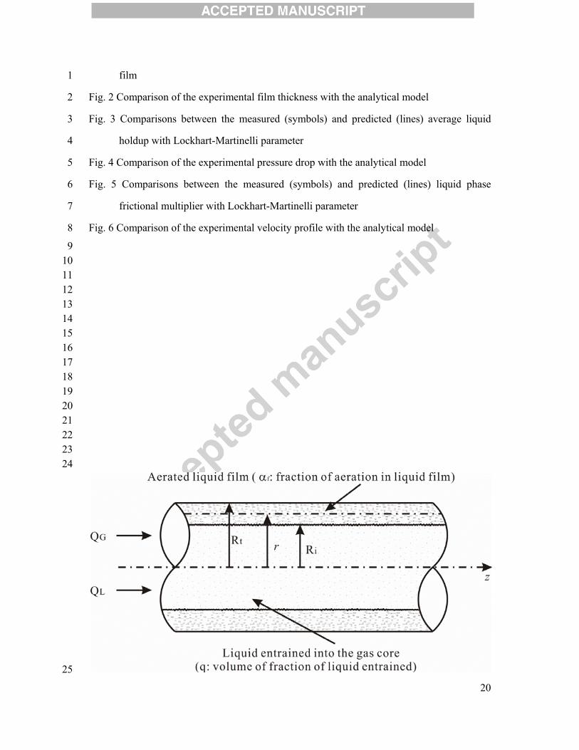
3.1 Film thickness 15

The comparison between the analytical model and published experimental results is 16

shown in Fig. 2. In the comparison, the average value of the measured thickness is used. The 17

predicted film thickness is determined by Eq. (32). The flowrates of gas and liquid follow the 18

information of previous experiments (Ashwood, 2010). The comparison shows that the 19

analytical model can predict the film thickness within the error of 10%' .20

3.2 Liquid holdup 21

The aeration and entrainment phenomenon were shown in the visual experiments 22

(Okawa et al., 2010; Ren et al., 2012). However there is inadequate experimental data about 23

these effects. The values of the aeration and entrainment are assumed. 24

To validate the predict liquid holdup over a range of flow conditions, comparisons are 25

15

made with available experimental results published(Shu, 1981). Figure 3 presents 1

comparisons between the measured (symbols) and predicted (lines) average holdup variations 2

with the Lockhart-Martinelli parameter (X). In the calculation of Newtonian fluids (n = 1), 3

the aeration and entrainment are set to be 0q and 0f� . The excellent agreement 4

shows that the effects aeration and entrainment is not significant for Newtonian flow. This 5

conclusion agrees well with the previous works. (Schubring and Shedd, 2009a; Shu, 1981). 6

The comparison of the predicted holdup for air–water experiments shows that the discrepancy 7

increases when viscosity of aqueous increases. As the liquid film viscosity increases, the 8

liquid film of aqueous can be highly aerated by small gas bubbles, hence the viscosity of 9

liquid film is lower than that of pure liquid. For the non-Newtonian flows (0.063 wt% 10

Separan, 0.125 wt% Separan, and 0.5 wt% Separan), the results show that the predicted 11

average holdup is higher than the measured values. The discrepancy increases with the 12

decrease of flow behavior index n due to the zero aeration and entrainment assumption. 13

In the experiments (Schubring and Shedd, 2009a), the actual degrees of aeration and 14

entrainment are unknown. Therefore the quantitative comparisons between analytical model 15

and experimental results are difficult to obtain. Figure 3 shows the results when the entrained 16

liquid fraction is q = 0.05 and void fraction is f� = 0.05. The model can predict the 17

observed trend of the experiments. The divergence between the model and the experimental 18

results can be improved by changing the values of aeration and entrainment. 19

20

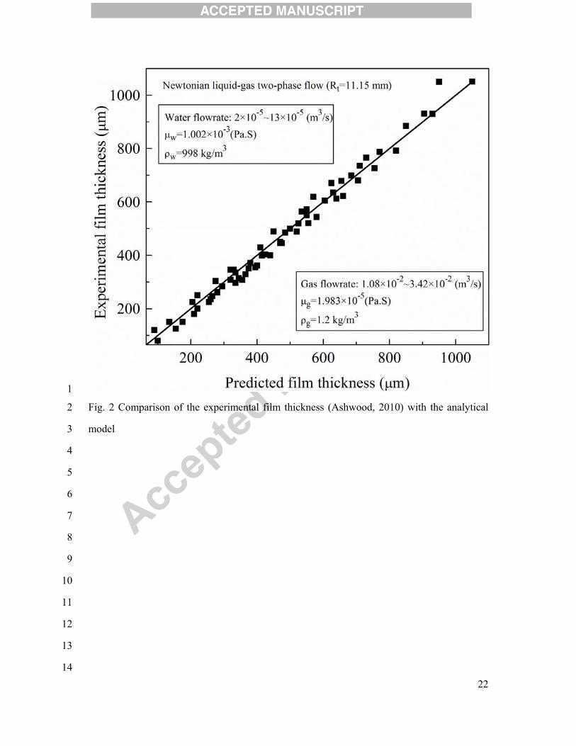
3.3 Pressure gradient 21

Figure 4 compares the predicted pressure gradient and experimental results from Brill 22

and Begss [2]. The experiments used various non-Newtonian fluids. The diameter of the pipe 23

is 0.01825 m. The flow behavior index changes from n = 0.43 to n = 0.76; the flow 24

consistency index changes from 3 20.62 10 N snm m� ( � to 3 240.3 10 N snm m� ( � .25

The superficial liquid Reynolds number (Re) ranges from 0.36 to 2,816. The gas Reynolds 26

number ranges from 1,339 to 45,727. The results show that the analytical model can predict 27

16

the measured pressure drop; the maximum difference between the model and the 1

experimental results is 15%. The error increases as the index n decreases. According to the 2

conclusion of Tyagi and Srivastava (Tyagi and Srivastava, 1976), the interface phenomenon 3

becomes more complex as the decrease of the flow behavior index n. Due to the perturbation 4

of pressure which leads to non-uniform radial pressure, and the pressures of two phases are 5

unequal. 6

7

3.4 Frictional multiplier 8

Figure 5 presents comparisons between the measured (symbols) and predicted liquid 9

phase frictional multiplier variations with the Lockhart-Martinelli parameter. The model 10

agrees reasonable well with the experimental results. For a given value of the 11

Lockhart-Martinelli parameter, decreasing the value of n gives a lower multiplier L� .12

Furthermore, the value of L� decreases with an increase of Lockhart-Martinelli parameter X.13

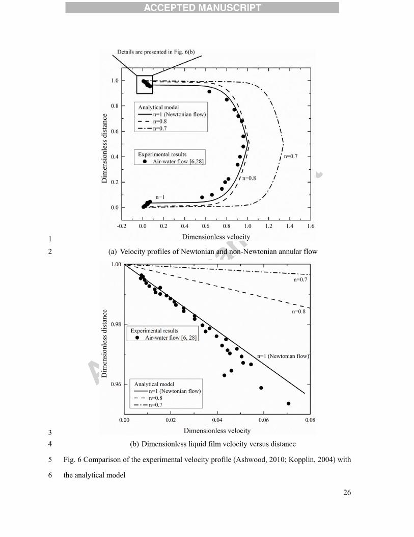
3.5 Velocity profiles 14

Figures 6 (a) and (b) show velocity profiles of Newtonian and non-Newtonian annular 15

flow in a horizontal pipe. The predicted velocity profile of air-water (Newtonian flow) 16

annular flow is compared with the experiments (Ashwood, 2010). In the experiments, the 17

diameter of the pipe is 0.0115 m, the gas flowrate is 0.01 m3/s, and the liquid flowrate is 18

53.6 10�( m3/s. The dimensionless distance and velocity are defined as follows 19

LRD

(48) 20

sg

UUU

(49) 21

where D is the diameter of the pipe and Usg is the superficial gas velocity. 22

The gas core velocity profile varies relatively smooth except in the region of the 23

vapor-liquid interface. In the most region of gas core, the velocity is uniform. The velocity 24

varies sharply within the interfacial region as can be seen from Fig. 6(a). 25

Figure 6 (b) shows the velocity profile of the liquid film. The velocity exhibit a linear 26

17

behavior throughout their profiles which indicates that the entire film regions are dominated 1

by the viscous behavior. The model agrees well with the experiments (Kopplin, 2004). The 2

results also show that under the same flow conditions, the film thickness decreases whereas 3

the film velocity increases with decreasing index n. For the shear-thinning power-law liquid, 4

the shear stress decreases with the velocity gradient. The shear stress is reduced for lower 5

values of n. Under the same flowrate, the flow with lower n is faster and the thickness is 6

thinner. At the same time, the lower shear stress at the interface causes lower pressure loss 7

due to friction, and consequently the gas phase flows faster. 8

9

4. Conclusions 10

A method is introduced to predict the pressure drop and film thickness of a 11

non-Newtonian two-phase annular flow based on the flowrates of liquid and gas. In the 12

model, the non-Newtonian fluid is described using power-law liquid. The logarithmic 13

velocity distribution is chosen to describe the turbulent gas core velocity profile. The 14

influences of entrainment and aeration are included in the model. 15

The results show that the model can predict the film thickness and pressure drop. The 16

variation between the analytical model and the experimental results is lower than 10%. The 17

shear-thinning effect influences the flow behavior. Comparing with the Newtonian flow, 18

under the same flowrates, the non-Newtonian two-phase flow experiences a lower pressure 19

drop and the flow behavior is more complex. Under the same flowrates, the film thickness of 20

non-Newtonian flow is thinner. 21

22Acknowledgement 23

The authors gratefully acknowledge research support from the Agency for Science, 24

Technology and Research (A*STAR) and Engineering Research Grant, SERC Grant No: 25

1021640147. 26

27

28

References 29Agrawal, S.S., Gregory, G.A., Govier, G.W., 1973. An analysis of horizontal stratified 30

18

two-phase flow in pipes. Canadian Journal of Chemical Engineering 51, 280-286. 1Al-Kizwini, M.A., Wylie, S.R., Al-Khafaji, D.A., Al-Shamma'a, A.I., 2013. The monitoring 2of the two phase flow-annular flow type regime using microwave sensor technique. 3Measurement: Journal of the International Measurement Confederation 46, 45-51. 4Al-Sarkhi, A., Sarica, C., Qureshi, B., 2012. Modeling of droplet entrainment in co-current 5annular two-phase flow: A new approach. International Journal of Multiphase Flow 39, 621-28.7Ashwood, A.C., 2010. Characterization of the macroscopic and microscopic mechanics in 8vertical and horizontal annular flow, Mechanical Engineering. University of 9Wisconsin-Madison. 10Baniamerian, Z., Mehdipour, R., Aghanajafi, C., 2012. Analytical simulation of annular 11two-phase flow considering the four involved mass transfers. Journal of Fluids Engineering, 12Transactions of the ASME 134. 13Brill, J.P., Begss, H.D., 1978. Two-phase Flow in Pipes. The University of Tulsa, Tulsa, Okla. 14Cioncolini, A., Thome, J.R., 2012. Void fraction prediction in annular two-phase flow. 15International Journal of Multiphase Flow 43, 72-84. 16Eisenberg, F.G., Weinberger, C.B., 1979. Annular two-phase flow of gases and 17non-Newtonian liquids. AIChE Journal 25, 240-246. 18G. F. Hewitt, N.S.H.T., 1969. Annular Two-Phase Flow. Pergamon Press,. 19Gazley, C., 1949. Interracial Shear and Stability in Two-phase Flow. University of Delaware, 20Newark. 21Hurlburt, E.T., Fore, L.B., Bauer, R.C., 2006. A Two Zone Interfacial Shear Stress and Liquid 22Film Velocity Model for Vertical Annular Two-Phase Flow, ASME 2006 2nd Joint 23U.S.-European Fluids Engineering Summer Meeting Collocated With the 14th International 24Conference on Nuclear Engineering (FEDSM2006) ASME, Miami, Florida, USA, pp. 25677-684. 26Kopplin, C.R., 2004. Local liquid velocity measurements in horizontal, annular two-phase 27flow. University of Wisconsin-Madison, Madison, Wisconsin, USA. 28Landel, R.F., B. G. Moser, A. J. Bauman, 1963. Proceedings of the Fourth International 29Congress on Rheology, in: Copley, A.L. (Ed.), Proceedings of the Fourth International 30Congress on Rheology. Brown University, New Yoke. 31Lockhart, R.W., Martinelli, R.C., 1949. Proposed correlation of data for isothermal two-phase, 32two-component flow in pipes. Chemical Engineering Progress 45, 39-48. 33Okawa, T., Goto, T., Yamagoe, Y., 2010. Liquid film behavior in annular two-phase flow 34under flow oscillation conditions. International Journal of Heat and Mass Transfer 53, 35962-971. 36Owen, D.G., Hewitt, G.F., 1987. An improved annular two-phase flow model. 37Ren, S.J., Tan, C., Dong, F., 2012. Two phase flow visualization in an annular tube by an 38electrical resistance tomography, pp. 488-492. 39Rodriguez, J.M., 2009. Numerical simulation of two-phase annular flow. Rensselaer 40Polytechnic Institute, New York. 41Schubring, D., Shedd, T.A., 2008. Wave behavior in horizontal annular air-water flow. 42

19

International Journal of Multiphase Flow 34, 636-646. 1Schubring, D., Shedd, T.A., 2009a. Critical friction factor modeling of horizontal annular 2base film thickness. International Journal of Multiphase Flow 35, 389-397. 3Schubring, D., Shedd, T.A., 2009b. Prediction of wall shear for horizontal annular air-water 4flow. International Journal of Heat and Mass Transfer 52, 200-209. 5Schubring, D., Shedd, T.A., 2011. A model for pressure loss, film thickness, and entrained 6fraction for gas-liquid annular flow. International Journal of Heat and Fluid Flow 32, 7730-739. 8Schubring, D.L., 2009. Behavior interrelationships in annular flow. University of 9Wisconsin-Madison, Madison, Wisconsin. 10Shedd, T.A., Newell, T.A., 2004. Characteristics of the liquid film and pressure drop in 11horizontal, annular, two-phase flow through round, square and triangular tubes. J. Fluids Eng. 12126, 807-817. 13Shu, M.T., 1981. Horizontal Two-phase Flow of Gases and Non-Newtonian Liquids. Drexel 14University, Philadelphia, p. 271. 15Srivastava, R.P.S., 1977. Liquid film thickness in annular flow. Chemical Engineering 16Science 28, 819-824. 17Srivastava, R.P.S., Narasimhamurty, G.S.R., 1973. Hydrodynamics of non-Newtonian 18two-phase flow in pipes. Chemical Engineering Science 28, 553-558. 19Tai, C.F., Chung, J.N., 2010. A direct numerical simulation of annular two-phase laminar 20flow and heat transfer in a circular pipe. International Journal of Computational Methods in 21Engineering Science and Mechanics 11, 230-246. 22Taitel, Y., Dukler, A.E., 1976. A model for predicting flow regime transitions in horizontal 23and near horizontal gas-liquid flow. AIChE Journal 22. 24Tyagi, K.P., Srivastava, R.P.S., 1976. Flow behaviour of non-Newtonian liquid-air in annular 25flow. The Chemical Engineering Journal 11, 147-152. 26Wallis, G.B., 1969. One-dimensional two-phase flow. McGraw-Hill, New York. 27Wang, R., Lee, B.A., Lee, J.S., Kim, K.Y., Kim, S., 2012. Analytical estimation of liquid film 28thickness in two-phase annular flow using electrical resistance measurement. Applied 29Mathematical Modelling 36, 2833-2840. 30Xiao, R., Wei, B., Chen, G., Xun, H., 2011. The calculation on liquid holdup in horizontal 31gasliquid two-phase annular flow, pp. 5362-5364. 32Xu, J.y., Wu, Y.x., Shi, Z.h., Lao, L.y., Li, D.h., 2007. Studies on two-phase co-current 33air/non-Newtonian shear-thinning fluid flows in inclined smooth pipes. International Journal 34of Multiphase Flow 33, 948-969. 35

3637383940

List of figures 41

Fig. 1 Model of annular flow with liquid entrainment into gas core and aeration in the liquid 42

20

film 1

Fig. 2 Comparison of the experimental film thickness with the analytical model 2

Fig. 3 Comparisons between the measured (symbols) and predicted (lines) average liquid 3

holdup with Lockhart-Martinelli parameter4

Fig. 4 Comparison of the experimental pressure drop with the analytical model 5

Fig. 5 Comparisons between the measured (symbols) and predicted (lines) liquid phase 6

frictional multiplier with Lockhart-Martinelli parameter 7

Fig. 6 Comparison of the experimental velocity profile with the analytical model 8

9101112131415161718192021222324

25

21

1

Fig. 1 Model of annular flow with liquid entrainment into gas core and aeration in the liquid 2

film 3

456789

101112131415161718192021222324252627

28

22

1

Fig. 2 Comparison of the experimental film thickness (Ashwood, 2010) with the analytical 2

model 3

4

5

6

7

8

9

10

11

12

13

14

23

1

2

Fig. 3 Comparisons between the measured (symbols) and predicted (lines) average liquid 3

holdup with Lockhart-Martinelli parameter4

5

24

1

Fig. 4 Comparison of the experimental pressure drop (Brill and Begss, 1978) with the 2

analytical model 3

4

5

6

7

8

9

10

11

12

13

14

25

1Fig. 5 Comparisons between the measured (symbols) and predicted (lines) liquid phase 2

frictional multiplier with Lockhart-Martinelli parameter 3

4

5

6

7

8

9

10

11

12

13

14

26

1(a) Velocity profiles of Newtonian and non-Newtonian annular flow 2

3(b) Dimensionless liquid film velocity versus distance 4

Fig. 6 Comparison of the experimental velocity profile (Ashwood, 2010; Kopplin, 2004) with 5

the analytical model 6

27

1

2

Highlights 3

1. An analytical model to predict non-Newtonian liquid-gas annular flow. 42. This model predicts the film thickness and pressure gradient at the same time only based 5on the flow rates of liquid and gas. 63. The influence of entrainment and aeration are predicted. 74. The difference between the model and the experimental results is lower than 10%. 8