A SIMPLE METHOD TO FOLLOW POST-BUCKLING PATHS IN FINITE ... · A SIMPLE METHOD TO FOLLOW...

Pergamon 0045-7949(94)00623-7

Compulm & Srrucrures Vol. 57. No. 3. pp. 477-489, 1995 Elsevier Science Ltd

Printed in Great Britam 0045.7949195 $9.50 + 0.00

A SIMPLE METHOD TO FOLLOW POST-BUCKLING PATHS IN FINITE ELEMENT ANALYSIS

B.-Z. Huang and S. N. Atluri

FAA Center for Excellence for Computational Modeling of Aircraft Structures, Georgia Institute of Technology, Atlanta, GA 30332-0356, U.S.A.

(Received 9 March 1994)

Abstract-A simple method to follow the postbuckling paths in the finite element analysis is presented. During a standard path-following by means of arc-length method, the signs of diagonal elements in the triangularized tangent stiffness matrix are monitored to determine the existence of singular points between two adjacent solution points on paths. A simple approach to identify limit or bifurcation points is developed using the definition of limit points and the idea of generalized deflections. Instead of the exact bifurcation points, the approximate bifurcation points on the secants of the solution paths are solved. In order to follow the required postbuckling branches at bifurcation points, the asymptotic postbuckling solution at the approximate bifurcation points, and the initial postbuckling behavior based on Koiter’s theory are given and used for the branch-switching. Some numerical examples of postbuckling behavior of metallic as well as laminated composite structures are computed using a “quasi-conforming” triangular shell element to demonstrate the proposed method.

1. INTRODUCHON

Nonlinear finite element method, as an effective analysis approach, has been widely used in structural postbuckling problems. Because there exist singular points on solution paths, the postbuckling analysis becomes complicated and difficult. It is well known that singular points are classified into two types, i.e. limit and bifurcation points. Correspondingly, there are two kinds of structural bucklings, i.e. snap-through (limit point, collapse) and bifurcation buckling. In the practical engineering structures, most of the buckling problems are snap-through due to the nonlinearity of prebuckling states and imperfections in geometry or loading of systems. In the linear or quasi-linear cases, the snap-through buckling result- ing from small imperfections of systems is the charac- teristic of the bifurcation of the corresponding perfect systems [l]. Usually, systems with linear or quasi- linear prebuckling states are an aim in the design of plate/shell structures due to their efficiency. Therefore, bifurcation buckling has received more attention in buckling/postbuckling theories and computational strategies. Many investigations in this field have been carried out from two aspects, the continuum mechanics and computational mathematics.

The basic approach to solving the nonlinear responses is the incremental iterative method or the continuation method, also called path-following method. The approach is based on the Newton method (or modified-Newton or quasi-Newton method). The Newton iteration method is good in its convergence, if the initial solutions used for iteration

are close to the solution paths. In order to obtain the approximate initial solution, a known adjacent solution point is usually necessary. Thus, the approach to solve nonlinear response is a process to follow solution paths step by step, starting from a known point, usually being the unloaded states. The step- length parameter can be chosen to be the load factor, a component of the displacement vector or a variable dependent on the load factor and the displacement vector (i.e. the so-called arc-length). The load-control incremental method fails to pass the limit points. In general, the various arc-length methods are considered the most effective [2-51 even for complicated paths.

The incremental iteration method cannot be directly used for the computation of singular points on the paths. But the existence of singular points between the adjacent solution points can be found by the inspection and comparison of the tangent stiffness matrices. When following the paths only with limit points, the results provided by arc-length methods are enough for the whole path calculation. If the singular point is a bifurcation point, the computation of the eigenvalue problem is usually necessary to follow a required branch after the bifurcation. In order to determine accurately the singular points and to identify the limit or bifurcation points, a direct algor- ithm was developed and used in finite element analysis [6, 71. In this procedure, the so-called extended systems, including the nonlinear equations and the constraint conditions about the singular points, are solved. In addition some simple methods are developed [8-IO], using the singularity of the tangent stiffness matrix.

478 B.-Z. Huang and S. N. Atluri

To follow a required branch at the bifurcation point, according to the convergence condition of Newton’s method mentioned before, the initial solution used for the iteration must be an approximate point near this branch. Perturbation methods are used for the branch switching [8, 11, 121. The basis of the methods is the asymptotic postbuckling theory found by Koiter [13].

In this paper, a simple method to follow the postbuckling paths in finite element analysis is presented. The detection and identification of singular points is based on the singularity of the tangent stiffness matrix and the definition of limits points, using so- called generalized deflection [l, 141 as a measure of deformation. Some properties of generalized deflection are discussed. Once the existence of bifurcation point between two adjacent solution points is determined, the approximate bifurcation point on the secant through the two solution points is calculated using the inverse power method. The asymptotic postbuckling solution on the locally linearized paths and initial postbuckling behavior based on Koiter’s theory is used for the branch switching. Using a “quasi-conforming” triangular shell element, some numerical examples are computed to evaluate the effectiveness of the proposed method.

2. BASIS OF ELASTIC POSTBUCKLING ANALYSIS

2.1. Potential energy functional

Suppose that we consider an elastic conservative system under proportional loading. The total potential energy functional can usually be written as

P(u, 1) = U(u) - AS(u), (1)

in which u is the displacement vector, 1 the load factor, U the strain energy and -LB the potential of external load.

We restrict attention here to semilinear elastic materials undergoing large deformation. In these materials, the strain measure and its conjugate stress measure are assumed to be linearly related.

Based on the total Lagrangean description, the strain energy U can be expressed by

U(u) =; s o :L dV, ”

(2)

where 0 is the second Piola-Kirchhoff stress tensor and L is the Green strain tensor with reference to the unloaded state. The constitutive equations are written as

u =H:e, (3)

where H is the elastic tensor. The strain tensor L can be expressed in the form

c = Cl (4 + I*, (4)

where L,(U) and L?(U) are the linear and quadratic terms of u, respectively. Likewise, using eqn (3), we have

u = u,(u) + az(u). (5)

2.2. Equilibrium and stability

If (u, 1) is a given solution point on the path, the potential energy functional at point (u + 4, A) is expanded with respect to 5 as follows

P(u + L A) = P(u, A) + P,(L 2)

+Pz(C,J)+PI(LA)+... (6)

in which c is a variation of the displacement u and P,,, is the mth variation of the functional P, which, according to the Gateaux definition, is expressed as

pm2 am m! at,...ac,

xP(u+~,u,+...+~,u,)l,,=. .=6mE0, (7)

where L+, (j = 1, . , m) are the variations of displacement u.

The condition of stationarity for P leads to the equilibrium equations at point (u, A)

p, (LA) = 0 (8)

or 6P(u, 1) = 0.

The sufficient and necessary condition of the stability of the equilibrium state (u, 1) is [l, 131:

AP({, A) = P(u + c, 1) - P(u, A)

= P,(L 1) + P,(<, 2) + ‘. 2 0. (9)

The sufficient condition is

P*(C, J-1 > 0, (10)

i.e. P, is positive definite. The necessary condition is

(11)

In finite element method, P2([, I) is usually expressed in the form

Pz(C, A) = q’K,q, (12)

where q is the generalized displacement vector for C and KT is the so-called tangent stiffness matrix.

2.3. Singular points

If the second variation P*(t;, k) at the point (u, A) is positive semi-definite, i.e. there exists 4, which

Simple method to follow post-buckling paths 479

satisfy the equation

P2 (C, , I) = min = 0 (I = 1 . . . M), (13)

then the point is called the singular point or the critical point. 1, denoted by A,,, is the critical load factor and 1;, the buckling modes.

The minimum condition eqn (13) leads to the variational equation

The incremental solution (Au, AL) satisfies the extended equations

6p,(r,1)=p,,(c,,6r,1,,)=0 (14)

where P,, is the bi-linear functional corresponding to P2. The finite element form of eqn (14) can be written as

which are the basic equations of the arc-length method. The different constraint conditions corre- spond to the different types of the arc-length method. Equation (20) can be expressed in finite element form

(21)

Krq, = 0, (15)

where q, is the generalized displacement vector for 4,. The condition eqn (13) means that at the singular point, KT becomes singular,

where Aq is the generalized displacement vector for Au, F the reference load vector.

2.5. IdentiJication of singular points

If (II, 2) is a singular point, assuming Au = al;, - 0 and A1 --+ 0 and using eqn (19), we have the equilibrium equation in the vicinity of the point (II, 1)

det K, = 0. (16)

In the following we will consider only the simple buckling case (M = 1).

2.4. Incremental equilibrium equation

For most structures, B(u) in eqn (1) is linear functional of II, given by

B(u)=~~~-udY+~~~I.udS (17)

where b and F are the body force and the known surface traction, respectively. 5 can be considered as an incremental displacement from the known solution II, and is denoted by

6 (AP) IAu = a(, +o.~-+o = a2P2(&) - adM([,) = 0. (22)

Considering eqn (13) the following condition is obtained:

dM(c,) = 0. (23)

Therefore, the well-known condition to identify the singular points can be written as

B([,) = FTq, = 0 (for bifurcation points)

B([,) = FTq, # 0 (for limit points). (24)

Au=&

If 2 in eqn (6) is replaced by 1 + Al, and Au and Al are assumed to be constrained by the condition

f(Au, AA) = 0, (18)

2.6. Generalized defection

The functional B(u) in the potential energy eqn (1) is called generalized deflection [I, 141. Physically, it represents the work done by the reference load system acting along the displacement field u

B(u)=lr-udY+~~~i.udS=FTq. (25)

considering eqn (17), eqn (6) can be expressed in From eqn (1) taking the partial derivative with

the form respect to 1, we have

P(u + Au, 1 + AL) = P(u, 1 + An) + P2(Au)

+ P3(Au) +. * . - ALB(Au)

or

E(u) = -; P(“, A). (26)

It can be proved (see Section 4) that u can be written in the following form in the vicinity of the bifurcation point

AP(Au, An) = P(u + Au, 1+ AA) - P(u, 1+ A1)

= Pz (Au) + P, (Au) + . . - AA&Au).

(19)

u(L) = u,(l) + al;, + 0(a*), (27)

where u,,(L) is the fundamental path. The increment of the potential energy functional [eqn (9)] can be


expanded with respect to A: at A,,

AP([, A) = P(u, + 5, A) - WI,,, i) = P,(C, j.,,)

+ P3(5, i,,) + + P4(& &,) + (28)

Substituting < = ai, + v [where vO(a’)] into eqn (28) and using eqns (13) and (14) we have

P(u, A) = P(u,, I.) + P2(v, j”,,)

+ P3(a5, + v, 4,) + P,(aC, + v, &,)

+ O((A. - ?._)a’, (2 - &.r)za2, a*). (29)

Substituting eqn (29) into eqn (26) the generalized deflection on the postbuckling branch can be given

by 1141

B(u)=B(u,,)-o'~P2(ii,i)li_i,,

+ O(u',u*(i -A_)). (30)

If the equilibrium is stable (when i ==c &,), the condition eqn (I 0) leads to

Noticing P*(<,, i,.) = 0 [see eqn (13)], the slope of the continuous function PZ(<, , i) at the bifurcation point i.,, should be

Therefore

W(i)) > W,(i)) (31)

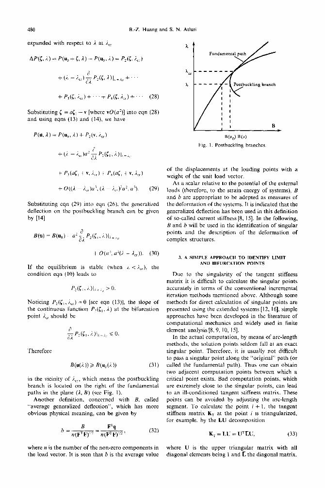
in the vicinity of I.,,, which means the postbuckling branch is located on the right of the fundamental paths in the plane (1, B) (see Fig. 1).

Another definition, concerned with B, called “average generalized deflection”, which has more obvious physical meaning, can be given by

B FTq b=-=- n(FTF)“* n(F“F)‘.‘* ’ (32)

where n is the number of the non-zero components in the load vector. It is seen that b is the average value

W,) B (4

Fig. 1. Postbuckling branches

of the displacements at the loading points with a weight of the unit load vector.

As a scalar relative to the potential of the external loads (therefore, to the strain energy of systems), B and b are appropriate to be adepted as measures of the deformation of the systems. It is indicated that the generalized deflection has been used in this definition of so-called current stiffness [8, 151. In the following, B and b will be used in the identification of singular points and the description of the deformation of complex structures.

3. A SIMPLE APPROACH TO IDENTIFY LIMIT AND BIFURCATION POINTS

Due to the singularity of the tangent stiffness matrix it is difficult to calculate the singular points accurately in terms of the conventional incremental iteration methods mentioned above. Although some methods for direct calculation of singular points are presented using the extended systems [12. 161, simple approaches have been developed in the literature of computational mechanics and widely used in finite element analysis [8,9, 10, 151.

In the actual computation, by means of arc-length methods, the solution points seldom fall at an exact singular point. Therefore, it is usually not difficult to pass a singular point along the “original” path (or called the fundamental path). Thus one can obtain two adjacent computation points between which a critical point exists. Bad computation points, which are extremely close to the singular points, can lead to an ill-conditioned tangent stiffness matrix. These points can be avoided by adjusting the arc-length segment. To calculate the point i + 1, the tangent stiffness matrix K, at the point i is triangularized, for example, by the LU decomposition

K,=LU=UTLU, (33)

where U is the upper triangular matrix with all diagonal elements being 1 and L the diagonal matrix.


The second variation of the potential energy of systems [see eqn (12)] can be expressed by

P&, a) = yTEy = i I,yf, (34) i--l

where Iii (no sum on i) are the diagonal elements of L, yi the components of the vector y = Uq and N the total degree of freedom. Thus, from eqns (IO), (1 l), (13) and the quadratic form (34) we obtain the stability conditions of solution points as follows.

The sufficient conditon for stability is

iii > 0 Vi 3 [I, N]. (35)

The necessary condition for stability is

l,,>O Vig[l, N]. (36)

The sufficient condition for instability is

Ii,<0 3i3[l, N] (37)

and the sufficient and necessary condition for the existence of the singular points is

l),=o 3i3[1,N]. (38) A&=1,+,-- 1,, AI,_,=li-l,_I.

The diagonal elements of L are continuous functions of the path parameter on solution paths. Therefore, the existence of singular points between two adjacent computation points can be easily determined by monitoring the sign changes of the diagonal elements Iii. If there is only one sign change there exists one singular point, a limit or a simple bifurcation point. The procedure will be carried out after each solution point has been computed, and the LU decomposition will be used in the calculation of the next point.

From the viewpoint of engineering application, the exact critical point is not always needed. However, the identi~cation of the limit or bifurcation points is necessary in order to follow postbuckling paths. If only limit points exist, the normal arc-length approach works, but if the singular point is a bifurcation point, the buckling analysis has to be carried out. Suppose that a singuiar point S is located between two known adjacent solution points i and i -I- 1. Using the condition dl = 0 at the limit point, instead of the condition eqn (24), which is dependent on eigenvector c,, the identification can be carried out in a simpler way.

It is assumed that there is only one singular point between point i and i + 1, and that li_, , li and A,, , are the load factors of point i - 1, i and i + 1, respectively. Consider the solution paths in the plane (1, B) (see Fig. 2). Let

S

S l . i+i i’ .

/

l -•. /

i ‘* i-l i+1

/ l i-l \

l i i+l

;y I

,* i-l

(4 (b)

(d) (e>

s l ‘i+l l $r

th)

(c)

6)

Fig. 2. Identification of Iimit and bifurcation points.


Obviously, if Ai,_, Ali < 0, the singular point S is point exists have been obtained, using the secant a limit point (maximum as in Fig. 2a or minimum as through points i and i -I- 1, the nonlinear path between in Fig. 2b). This is the simplest situation. i and i + 1 can be linearized as follows:

If Al, _ , . AI, > 0, both the limit and the bifurcation points are possible. In this case, it is necessary to compute another point i’, between point i and i + 1 and close enough to i + 1, by slightly decreasing the arc-length segment between i and i + 1. The difference AL,, = 1,. - 1, may be used for further identification.

u,(l) = II, + ~Au, (40)

where

I= (A. - /I,)/@,+, - Ai). (41)

If ]A&.( 2 ]A&], S is a limit point (see Fig. 2c-f). If ]A& ] < (Ali] and there exists at least one sign

change in the diagonal elements I,, at point i’ in comparison with that at point i, the point S is a bifurcation point (Fig. 2g).

If 1 A&( < ]Ai,] and no sign change exists for any diagonal element, the generalized deflection B or the current stiffness will be used to obtain useful information for the identification of the singular points. On the path curves i - B, the slopes at limit points become zero and the slopes at bifurcation points nonzero. Hence, if point i’ is close enough to i + 1, in other words both i’ and i + 1 are close to the singular point, the following relations are valid:

On the linearized fundamental path u,,(J), the bifurcation point can be determined by a simpler method, so that it is not needed to approach to the exact bifurcation point gradually.

Consider an adjacent state near the fundamental state u,(L)

u=u,,(i)+c =u,+xAu,+[. (42)

Substituting u into eqn (4) we have

J=($~++~J/(~)==$l forlimitpoints

in which c,, is the symmetric bilinear form of cz. s = 1 for bifurcation points (39) Replacing u in eqn (6) by u, + ~Au, and using

eqn (43) the second variation P#, 1.) is obtained (see Fig. 2i and Fig. 2h). The experience of computation shows that the conditions eqns (39) are effective in most postbuckling analysis. P:(W=; [(a,(5)+2~,,(u,,5))(tl(r)

Once the existence of the bifurcation point between s Y

the point i and i + 1 is determined, we have to give an approximate solution for the required secondary branch in order to follow this branch. This is because the incremental iterative methods would “automatic- ally” follow the fundamental paths after bifurcation points, if the tangent of solution at the points was not changed. In the following section, Koiter’s asymptotic postbuckling theory is used to obtain the initial postbuckling solution in the vicinity of bifurcation points.

+ 2c,,(u,, C)) + 2(a,(u,) + a2(u,)k2(S)

+2~(2a,(&,,(Au,,O

+4a,,(u,,r)t,,(Au,,5)

+ ~i(Au,kz(O + 2a,,h> Au,kzK))

+ 2~‘(2a,,(Au,,r)t,,(Au,, 5)

4. APPROXIMATE ASYMPTOTIC POSTBUCKLING SOLUTION

+ ~2@4)~2(C))l dV. (44)

From eqns (14) and (4 l), eqn (15) can be written as

The asymptotic postbuckling theory was applied follows: to the study of initial postbuckling behavior in the vicinity of bifurcation points by means of analytical

i- [Kw + n(K), + ~Kw)lq = 0, (45)

or numerical methods [17, 181. The initial postbuckling behavior is “accurate” in an asymptotic sense. In the in which the matrices K,,, K,, and K,, are defined by following, the nonlinear fundamental state between two solution points near a bifurcation point is linearized to obtain the approximate asymptotic solution. ~qTK,i(a)q= [(~,(6r)+2a,,(u,,65))(c,(5)

s Y

4.1. Approximate bijiircation point + 2t,,(u,, 0) + 2(~,(U,)

If the solution points i (u,, Ai) and i + 1 (ui + Au,, 1, + AL,) between which an unknown bifurcation + c,(u,))t,,(X 01 dV


~q’K,,(Aq,,Aqih=2 [~~,,(Au~,~C)EII(AU~,~) s Y

+ 02(Auik,, (SC, 01 dvt (46)

where q, is the generalized displacement for ui. Because Aui is much smaller than II, and I< 1, the nonlinear eigenvalue problem can be solved by the inverse power method for linear problems

K,,q = I( -K,, - X’K,,)q, (47)

where p is the approximate eigenvalue in the last iteration. This procedure is not very time-consuming in general. Thus we can obtain the approximate critical load factor &, and the buckling mode 6, or q, . q, may be normalized by

qPo,q, = 1. (48)

4.2. Approximate asymptotic solution

In order to determine the initial postbuckling paths, according to Koiter’s method, the additional displacement vector 5 of the approximate fundamental state u,(L) [see eqn (42)] is expressed in the form

or in FE form

5 = aTI + v, (49)

Aq=aq, fp, (50)

where a is an unknown coefficient, v is a modified displacement vector and p is the generalized displacement for v, orthogonal to the buckling mode with the condition

qfK,,p = 0. (51)

Substituting eqn (49) into the expanded expression of the potential energy eqn (6), we obtain the increment of potential energy

Ap(q, 2) = J’(u, + 5, A) - P(u,, 2)

=(I-x,)u2A;,

+ (152 - Izr)a2A;, + A,& + B4a4

+ ~P~&,IP + a2pTFll

+ 0(a5, (X - &,)u3)

in which

A;L = fq:K,,q,

A ;N = fq:K,,q,

A, = -fq:F,,

B4 = idK2h 3 s,h

KM = hi + &(K,.c + LK,,v)

(52)

(53)

where the matrix K, and vector F,, are defined by

q:K,(q,,q,)q, =4 a,((, 162 (rl) d V

F,, = -iK,L(q, + &rAqi, q,)q,. (54)

Considering, first, a in eqn (52) as a constant and ignoring the high order small terms, from 6 (Ap(q, A)) = 0, p can be solved in the form

P = a2/&,, (55)

where p,, is the solution of the following equations

1

KXIP,, = F,,

pfi Koiq, = 0. (56)

It is noted that this extended linear equation set is not singular. Substituting eqn (55) into eqn (52) the increment of the potential energy is obtained as a function of the load factor L and the amplitude a of the additional displacement vector,

Ap(a,I)=(fi-&)aZA;,+(~2-~$)a2A;N

+A,a3+A,u4+O(a5,(~-_C,)a3) (57)

where

From

A~=B~-~P~IK,~,P,,. (58)

the relation between 1 and a is given by

2(1- &,)A;, + 2(z2 - xzr)A;,

+ 3A,u + 4A4a2 = 0. (59)


In the special case when A, = 0, the structures are usually called the “symmetric” or “quartic” structures. The structures are called “asymmetric” or “cubic” if

A,#O.

the approximate eigenvalues and the eigenfunctions can be solved using the inverse power method, which is not very time-consuming.

5. SWITCHING AND CALCULATING POSTBUCKLING BRANCHES

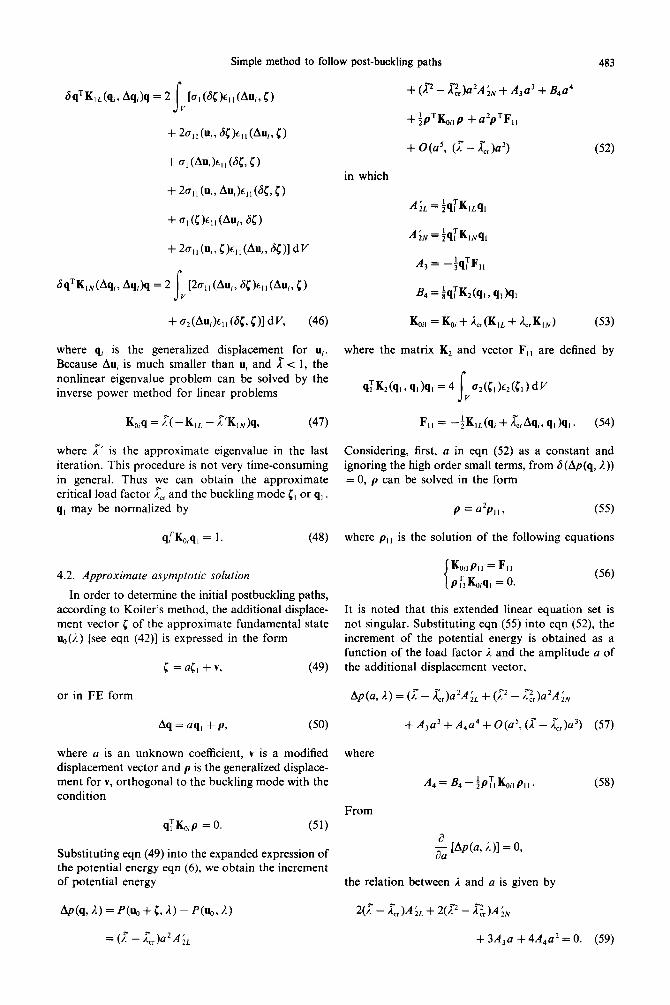
In this section, some numerical examples of plate/shell postbuckling are calculated using the finite element method to evaluate the effectiveness of the approach described in Sections 3-5. In all of the

As mentioned before, in order to follow a postbuckling branch at the bifurcation points, it is necessary to find an initial approximate solution near the postbuckling branch. The initial solution may be evaluated by the method in Section 4. In addition, because there are two (for simple buckling) or more (for multi-mode buckling) postbuckling branches at a bifurcation point, it is necessary to select the appropriate branch in engineering analysis. The asymptotic postbuckling theory can provide the needed guidance for the selection.

(a) Geometry

Generally, there will exist the descending branches for asymmetric structures, among which the sharpest / path corresponds to the most serious and, therefore, the most interesting case [19]. If the bifurcation point is simple buckling (M = I), one branch is descending while the other is ascending. For symmetric structures with simple buckling, there are two symmetric ascending branches if A, > 0, and two symmetric descending branches if A, < 0 (refer to Refs [13, 201 for further details).

(b) Load vs. deflection at center

16 - - Leicester (1968)

By means of the above mentioned conclusions, we can determine the branch to be followed and take a point B*(u,, &) on the approximate asymptotic path as the approximate solution for switching the postbuckling branch,

where Ah is a given load factor and (u,, A,), (II, + , , Ai+ ,) are two points on the fundamental paths near the bifurcation point. It is noted that the approximate bifurcation point S* is not the exact solution point, so that it should not be taken as the beginning of postbuckling branches. Therefore, the path-following for the postbuckling branch will start from the point near the bifurcation point on the fundamental paths. The Newton iteration method, based on load-control or arc-length control, can be used to calculate the first solution point B on postbuckling branches. Once the first solution point is obtained, the following solution points on the postbuckling branches can be solved using the standard arc-length methods.

wJt

(c) Sign change of iii

;:\ /- It is seen that the search for the exact solution

of the eigenvalue problems at bifurcation points is avoided in all of the procedures mentioned above, both in identification of singular points and in branch switching. The approximate solutions of the eigenvalue problems are needed only in the case where there exist bifurcation points. Due to the local linear- ization of the solution paths near bifurcation points,

-2 ( 0 0.5 2.0 2.5 1.0 1.5 3.0

Fig. 3. Square spherical cap under central loading. (a) Geometry. (b) Load vs deflection at center. (c) Sign

r .

6. NUMERICAL EXAMPLES

amem- Tahiam and Lachancc (1975) ;

-o_ Present 4x4 :

I I I I I I 0.5 1 .o 1.5 2.0 2.5 3.0

WC/t

cnange 01 lip.


examples, a “quasi~onfo~ing” triangular shear shell element is used, which is based on the Hu- Washizu variational principle and Koiter’s shallow shell theory under moderate rotation, with 7 degrees of freedom per node [21]. An arc-length method, in which the Euclidean norm ui * ui = const. is taken as the constraint condition, is adopted to follow the nonlinear paths [22]. Example 1 is the snap-through problem of a square spherical cap under central loading, which is often used to assess the accuracy of path-following in the nonlinear finite element analysis. Example 2 is the postbuckling of a plate subjected

(a) Geometry

(b) Load factor vs. deflection at center

1.8

1.6

1.2

s LI$ 1.0

5 0.8 0

0.6

0.4

0.2

0

- - Yemaki (1959)

4- Present 3x3

* Present 4x4

8 I I I I I I 0 0.5 1 .o 1.5 2.0 2.5 3.0

WC/l

(c) Load factor vs. displacement B‘ Loaded edge

1.8 r

1.6

1.4

17

- - Yamaki (1959)

+ Present 3x3

- Present 4x4 .._ % !$ 1.0

5 0.8 6

0.6

1.0

b (mm)

1.5 2.0

Fig. 4. Square plate under axial compression. (a) Geometry. Fig. 5. Stiffened plate under axial compression. (a) Geometry. (b) Load factor vs deflection at center. (c) Load factor vs (b) Load vs deflection at point C and B. (c) Load vs average

displacement at loaded edge. generalized deflection.

to axial compression. This is a classical postbuckling problem that can be solved analytically. In example 3 a stiffened plate with more complex postbuckling behavior is considerd. In example 4 a stiffened laminated panel under axial compression is computed.

6.1. Square spherical cap under central point load

Consider a square spherical cap, shown in Fig. 3a, under central loading, with all edges simply supported.

(a) Geometry

---

(b) Load vs. deflections at point C snd B

0.20 r

0.18

0.16

0.14

0.12

0.10

0.08

0.06

0.04

Point Branch

-x-C (2) --O--B (1) . -xv. B (2)

I .

0.02 0 1 I I I I I -2 0 2 4 6 8 10

* (mm)

(C) Load vs. average generalized deflection

0.20 r

Branch

-4- (1) -x- (2)


The geometry is taken as edge length a = 61.8034 in, radius R = 100 in and thickness t = 3.9154 in and the material properties are Young’s modulus E = 10 Psi, Poisson’s ratios v = 0.3. Due to a double symmetry, only a quarter of the cap is considered using 4 x 4 meshes. The curves of the deflection at center w, vs load P are given in Fig. 3b, in which the known results j23, 241 are contained to compare with the present result. The sign change of the diagonal elements iii in the matrix L is shown in Fig. 3b where the value I,,/lr,,I = - 1 corresponds to unstable

equilibrium and the value I,/lf,,l = 1 corresponds to stable equilibrium. The distribution of the computation points near limit points shows that the determinations of the maximum and minimum points are similar to the cases (d) and (b) in Fig. 2, respectively.

6.2. Square plate under axial compression

A square plate under axial compression, shown in Fig. 4a, is considered. All edges are simply supported, uniformly movable in the mid-surface and in-plane

(a) Buckling mode

(b) Branch (1) (C) Branch (2)

Fig. 6. Distribution of deflection. (a) Buckling mode. (b) Branch (1). (c) Branch (2)


shear stress free. The Poisson ratio of the materials is center and edge displacement are defined as aaZ/ taken as v = 0.333. A quarter of the plate with 4 x 4 (dTt2), w,./r and u/t, respectively. Due to the linearity meshes is computed due to the symmetry. This is a of the fundamental state, the bifurcation point symmetric structure with linear prebuckling behavior. obtained between two adjacent computation points As in general nonlinear problems, the path-following corresponds the exact critical load factor A,, = u,ra2/ starts with the unloaded state. The calculation results (aEt2) = 0.374. In general nonlinear cases, the bifur- and the analytical solutions [25] are shown in Fig. 4b cation points are approximate and are not considered and c, where the dimensionless load, deflection at as points on the solution paths.

(a) Geometry

w

(b) Load vs. deflections II point C and B

0.35 r

P Point Branch

---o-C (1) -+- c (2) - O- * B (1) _ .+- . B (2)

o- 0 5 10 15 20 25

w (mm)

(C) Load vs. avernge generalized deflection

0.35 r

H,’ @&+--jY s-z #*

0.15 - B Branch

e (1) -+- (2)

I I I I 0.5 1.0 1.5 2.0

b (mm)

Buckling mode

Branch (1)

Branch (2)

(d) Postbuckling deflection field

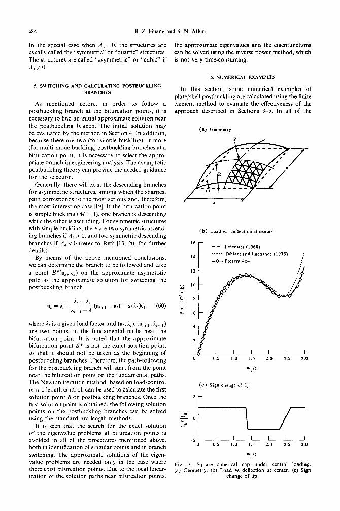
Fig. 7. Stiffened laminated panel under compression. (a) Geometry. (b) Load vs deflections at point C and B. (c) Load vs average generalized deflection. (d) Postbuckling deflection field.


6.3. St@ened plate under axial compression

In this example the postbuckling of a stiffened plate under axial compression is calculated. All edges are simply supported, the loaded edges are uniformly movable and the unloaded edges are stress free. The geometry and mesh of the plate are shown in Fig. Sa, where the sizes a = 1200 mm, b = 900 mm and the skin thickness r = I mm. The area, the out-off plane and in-plane moment of inertia, polar moment of inertia and eccentricity of the cross-section of stiffeners are A = 141 mm’, J = 16,895 mm4, J’ = 8206 mm“, JK = 423 mm4 and e = 7.85 mm, respectively. The cross-section of all stiffeners is assumed to be same. The material properties are taken as E = 65 kN mm2, v = 0.3. The results of the path-following are shown in Fig. 5b and c by means of the central deflection and average generalized deflection vs load factor, respectively. The first singular point is a symmetric and stable bifurcation point (A3 = 0. A, > 0). The buckling mode given in Fig. 6a shows that only the skin sections between stiffeners buckled (i.e. local buckling). After the bifurcation point there are two ascending branches which are all stable. Due to the influence of the eccentricity of stiffeners, the postbuckling branches are unsymmetric and obviously different from each other. Branch (2) corresponds to a smaller deflection than that of branch (1). With the growth of the buckling, the deflection of the skin increases rapidly, causing the growth of the stiffener bending (Fig. 6b, c and d) and leading to the collapse of the stiffened plate in the end. Because of the effect of nonlinearity, as in most of plate/shell structures, the second singular points on two branches are limit points. The maximum load of branch (2) is lightly higher than that of branch (I).

6.4. St~jf>ned punel under compression

A stiffened 16 layer [(O/90),], laminated panel with all edges simply supported under compression, meshed by 9 x 9 in a quarter. is considered. The sides of the panel and the cross-section of the stiffeners in x and J directions (see Fig. 7a) are taken as follows: cI = 1200mm, h =900mm. t =2mm, A =56mm’, J = 2843 mm4, J’ = 1160 mm4. JL = 74.67 mm4 and e = 5.482 mm. The material properties are assumed as E, = 135 GPa. Ez = 13 GPa, G,, = G,, = 6.41 GPa, G,, = 4.34 GPa. and 11,~ = 0.38. Assume that the reference load (i = I) acting on the panel leads to the strains t, = 0.001, c, = const.. ;‘,, = 0 and zero resultant forces along the whole edges y = *b/2 in the linear state. The postbuckling behavior is similar to that in example 3. At A,,= 0.121, a symmetric bifurcation buckling is obtained. On two different postbuckling branches exist the limit points i = 0.286 for branch (I) and E. = 0.303 for branch (2). The deflections at the center C and the mid-point B of the stiffener in the .Y direction, the average generalized deflection of the system and the postbuckling deflection field are shown in Fig. 7b-d, respectively.

It is seen that for the eccentrically stiffened plates under compression there usually exist two stable postbuckling equilibrium paths where both of them should be considered.

7. CONCLUDING REMARKS

In this paper a simple method to follow postbuckling paths of elastic conservative systems in finite element analysis is presented. Because both stability of equilibrium and existence of singular points depend on the second variation of the potential energy of systems, it is effective to monitor the sign and sign changes of the diagonal elements in the triangularized tangent stiffness matrix for determination of both stability of equilibrium and existence of singular points. According to the definition of limit points, the variation of load factor on the two sides of a singular point along the fundamental paths can be used for the identification of limit and bifurcation points. In some cases, it is necessary to compute an additional point, close to the solution point after the singular point, and to check the variation of the generalized deflection. The numerical experience shows that the approach is simple and effective even in the postbuckling analysis for complex structures. To follow the required postbuckling branches at bifurcation points an approximate analysis for the eigenvalue problems and the initial post-buckling is adopted. The approximate bifurcation points on the locally linearized fundamental paths and the initial postbuckling behavior are used for switching and selecting the critical branches. The proposed procedures, both for identification of singular points and for branch switching, can be carried out without too much additional computation.

Acknowledgements-This work was supported by a grant from the FAA to the Center of Excellence for Computational Modeling of Aircraft Structures at the Georgia Institute of Technology. The first author also wishes to express his thanks to the National Natural Science Foundation of China for its support.

1.

2.

3.

4.

5.

6.

REFERENCES

W. T. Koiter, Current trends in the theory of buckling. In Proc. IUTAM Symp. Buckling qf‘ Structures (Edited by B. Budiansky), pp. I-16 (1974). G. A. Wempner, Discrete approximations related to nonlinear theories of solids. Int. J. Solids Struct. 7, 1581-1599 (1971). E. Riks, An incremental approach to the solution of snapping and buckling problems. Int. J. Solids Struct. 15, 529-551 (1979). M. A. Crisfield, A fast incremental/iterative solution procedure that handles ‘snap-through’. Comput. Struct. 13, 55-62 (1981). E. Ramm, Strategies for tracing the nonlinear response near limit points, In Nonlineur Finite Element Analysis in Structural Mechanics (Edited by Wunderlish et al.). Springer, Berlin (1981). G. Moore and A. Spence, The calculation of turning points of nonlinear equations. SIAM J. numer. Anal. Comput. 17, 567-575 (1980).


7. P. Wriggers, W. Wagner and C. Miehe, A quadratically convergent procedure for the calculation of stability points in finite element analysis. Comput. Meth. appl. 17. mech. Engng 70, 329-347 (1988).

8. E. Riks, Some computational aspects of the stability 18. analysis of nonlinear structures. Comput. Meth. appl. Mech. Engng 47, 219-259 (1984).

9. W. Wagner and P. Wriggers, A simple method for the 19. calculation of oostcritical branches. Ennnp Comout. 5.

10.

11.

12.

13.

14.

15.

103-109 (1988). _- .

J. Shi and M. Crisfield, A simple indicator and switch- 20. ing technique for hidden unstable equilibrium paths. Finite Elements Anal. Des. 12, 303-312 (1992). G. A. Thurston, Continuation of Newton’s method through bifurcation points. J. appl. Mech. 36(3); Trans. 21. ASME 91, 425-430 (1969). W. Wagner, Nonlinear stability analysis of shells with the finite element method. In Nonlinear Analysis of Shells by Finite Elements (Edited by F. G. Rammerstorfer). 22. Springer, Vienna (1992). W. T. Koiter, On the stability of elastic equilibrium. Polytechnic Institute Delft, H. J. Paris Publisher, 23. Amsterdam 1945, NASA TT F-10. 833, 1967; and AFFDL-TR-70-25, 1970. 24. B. Budiansky, Theory of buckling and postbuckling behavior of elastic structures. Adu. appl. Mech. 14, l-65 (1974). 25. P. G. Bergan, G. Horrigmore, G. Krakeland and T. H. Soreide, Solution techniques for nonlinear finite element problems. Int. J. numer. Meth. Engng 12, 1677-1696 26. (1978).

16. P. Wriggers and J. C. Simo, A general procedure for the

direct computation of turning and bifurcation points. Int. J. namer. Meth. Engng 30, 155-176 (1990). J. W. Hutchinson and W. T. Koiter, Postbuckling theory. Appl. Mech. Rev. 23, 1353-1366 (1970). E. Carnoy, Postbuckling analysis of elastic structures by the finite element method. Comput. Meth. appt. mech. Engn,g 23, 143-174 (1980). D.- Ho, Buckling load of nonlinear systems with multiple einenvalues. Int. J. Solids Strut. 10. 1315-1330 (1974). - W. T. Koiter, General equations of elastic stability for thin shells. In Proc. Symp. Theory of She/Is in Honor of Lloyd H. Donnell (Edited by D. Muster), University of Houston, TX, pp. 187-227 (1967). B.-Z. Huang, V. B. Shenoy and S. N. Atluri, A quasi- conforming triangular laminated composite shell element based on a refined first-order theory. Comput. Mech. 13, 295-314 (1994). J. D. Zhang and S. N. Atluri, Postbuckling analysis of shallow shells by the field-boundary-element method. ht. J. numer. Meth Engng 26, 571-587 (1988). R. H. Leicester, Finite deformations of shallow shells. J. Eng. Mech. Div. ASCE 94, 140991423 (1968). C. Tahiant and L. Lachance, Linear and nonlinear analysis of thin shallow shells by mixed finite elements. Comput. Struct. 5, 167-177 (1975). N. Yamaki, Postbuckling behavior of rectangular plates with small initial curvature loaded in edge compression.

- J. A. M. 26, 407-414 (1959). W. C. Rheinboldt. Numerical analvsis of continuation methods for nonlinear structural problems. Comput - Strut. 13, 103-113 (1981).

A SIMPLE METHOD TO FOLLOW POST-BUCKLING PATHS IN FINITE ... · A SIMPLE METHOD TO FOLLOW...

Documents

Transcript of A SIMPLE METHOD TO FOLLOW POST-BUCKLING PATHS IN FINITE ... · A SIMPLE METHOD TO FOLLOW...