A SENSITIVITY ANALYSIS ON DEFINED BENEFIT ...benefit obligation under IAS 19 in Switzerland,...
79
UNIVERSITY OF LJUBLJANA SCHOOL OF ECONOMICS AND BUSINESS MASTER’S THESIS A SENSITIVITY ANALYSIS ON DEFINED BENEFIT OBLIGATION UNDER IAS 19 IN SWITZERLAND Ljubljana, September 2019 MIRJAM PERGAR
Transcript of A SENSITIVITY ANALYSIS ON DEFINED BENEFIT ...benefit obligation under IAS 19 in Switzerland,...

UNIVERSITY OF LJUBLJANA
SCHOOL OF ECONOMICS AND BUSINESS
MASTER’S THESIS
A SENSITIVITY ANALYSIS ON DEFINED BENEFIT OBLIGATION
UNDER IAS 19 IN SWITZERLAND
Ljubljana, September 2019 MIRJAM PERGAR

AUTHORSHIP STATEMENT
The undersigned Mirjam Pergar, a student at the University of Ljubljana, School of Economics and Business
(hereafter: SEB LU), author of this written final work of studies with the title A sensitivity analysis on defined
benefit obligation under IAS 19 in Switzerland, prepared under the supervision of doc. dr. Barbara Mörec
D E C L A R E
1. this written final work of studies to be based on the results of my own research;
2. the printed form of this written final work of studies to be identical to its electronic form;
3. the text of this written final work of studies to be language-edited and technically in adherence with the
SEB LU’s Technical Guidelines for Written Works, which means that I cited and/or quoted work and
opinions of other authors in this written final work of studies in accordance with the SEB LU’s Technical
Guidelines for Written Works;
4. to be aware of the fact that plagiarism (in written or graphical form) is a criminal offense and can be
prosecuted in accordance with the Criminal Code of the Republic of Slovenia;
5. to be aware of the consequences a proven plagiarism charge based on the this written final work could
have for my status at the SEB LU in accordance with the relevant SEB LU Rules;
6. to have obtained all the necessary permits to use the data and work of other authors which are (in written
or graphical form) referred to in this written final work of studies and to have clearly marked them;
7. to have acted in accordance with ethical principles during the preparation of this written final work of
studies and to have, where necessary, obtained the permission of the Ethics Committee;
8. my consent to use the electronic form of this written final work of studies for the detection of content
similarity with other written works, using similarity detection software that is connected with the SEB LU
Study Information System;
9. to transfer to the University of Ljubljana free of charge, non-exclusively, geographically and time-wise
unlimited the right of saving this written final work of studies in the electronic form, the right of its
reproduction, as well as the right of making this written final work of studies available to the public on the
World Wide Web via the Repository of the University of Ljubljana;
10. my consent to the publication of my personal data that are included in this written final work of studies
and in this declaration, when this final work of studies is published.
Ljubljana, ___________________ Author’s signature: ___________________

i
TABLE OF CONTENTS
INTRODUCTION ............................................................................................................... 1
1 EMPLOYEE BENEFITS UNDER INTERNATIONAL ACCOUNTING
STANDARD 19 .......................................................................................................... 3
1.1 Type of employee benefits .................................................................................... 4
1.2 Post-employment benefit plans ............................................................................ 5
1.2.1 Defined contribution plans .............................................................................. 5
1.2.2 Defined benefit plans ....................................................................................... 6
1.3 Defined benefit obligation .................................................................................... 6
1.3.1 Recognition ...................................................................................................... 8
1.3.2 Measurement ................................................................................................... 9
2 THE SWISS RETIREMENT SYSTEM .................................................................. 10
2.1 Old age, survivor's and disability insurance .................................................... 11
2.2 Occupational pension scheme ............................................................................ 12
2.2.1 Benefits .......................................................................................................... 13
2.3 Private pension scheme ...................................................................................... 15
3 ACTUARIAL ASSUMPTIONS ................................................................................ 15
3.1 The need for actuarial assumptions .................................................................. 15
3.2 Demographic assumptions ................................................................................. 17
3.2.1 Mortality rate ................................................................................................. 18
3.2.1.1 Mortality tables .......................................................................................... 19
3.2.1.2 Mortality improvements ............................................................................. 21
3.2.2 Disability rate ................................................................................................ 23
3.2.3 Employee turnover rate ................................................................................. 24
3.2.4 Lump sum payment or capital option ............................................................ 24
3.2.5 Conversion rate .............................................................................................. 25
3.3 Financial assumptions ........................................................................................ 26
3.3.1 Discount rate .................................................................................................. 27
3.3.2 Interest credit rate .......................................................................................... 29
3.3.3 Inflation ......................................................................................................... 30
3.3.4 Salary increase rate ........................................................................................ 30
3.3.5 Social security increase and pension increase ............................................... 31

ii
4 SENSITIVITY ANALYSIS ....................................................................................... 31
4.1 Selected assumptions .......................................................................................... 32
4.2 Description of the benefit plan used in the valuation ...................................... 35
4.3 Data and sample selection .................................................................................. 36
4.4 Benefit valuation tool.......................................................................................... 39
5 RESULTS ................................................................................................................... 43
5.1 Conversion rate ................................................................................................... 44
5.2 Capital option ...................................................................................................... 45
5.3 Loading factor on the turnover rate ................................................................. 46
5.4 Loading factor on disability rate ....................................................................... 47
5.5 Discount rate ....................................................................................................... 48
5.6 Interest credit rate .............................................................................................. 49
5.7 Salary increase rate ............................................................................................ 50
5.8 Overview of results ............................................................................................. 51
5.8.1 A practical example ....................................................................................... 52
5.8.2 Conversion rate, discount rate, and interest credit rate ................................. 55
5.8.3 Conversion rate and capital option ................................................................ 56
CONCLUSION .................................................................................................................. 57
REFERENCE LIST .......................................................................................................... 60
APPENDIXES ................................................................................................................... 65
LIST OF FIGURES
Figure 1: The Swiss three-pillar pension system ................................................................ 11
Figure 2: Life expectancy at birth in Great Britain ............................................................. 18
Figure 3: Life expectancy increase according to RP-2014 from RP-2000 ......................... 20
Figure 4: Effect of including projected mortality improvements on mortality tables ......... 21
Figure 5: Cohort life expectancies at age 65 according to different mortality improvement
models ................................................................................................................. 23
Figure 6: How parameter value deviation from the baseline values affects the DBO ........ 44
Figure 7: DBO for different conversion rates ..................................................................... 45
Figure 8: DBO for different capital options ........................................................................ 46
Figure 9: DBO for different loading factors on the turnover rate ....................................... 47
Figure 10: DBO for different loading factors on disability rate .......................................... 48
Figure 11: DBO for different discount rates ....................................................................... 49

iii
Figure 12: DBO for different interest credit rates ............................................................... 50
Figure 13: DBO for different salary increase rates.............................................................. 51
Figure 14: DBO for correlated scenarios between discount rate, conversion rate, and interest
credit rate ............................................................................................................ 56
Figure 15: DBO for correlated scenario between conversion rate and capital option ......... 57
LIST OF TABLES
Table 1: Determining the end value of a DBO ...................................................................... 7
Table 2: Determining the end value of plan assets ................................................................ 8
Table 3: Minimum retirement credits as prescribed by the BVG applicable on the mandatory
part of the second pillar pension ............................................................................ 14
Table 4: Most common parameter values of actuarial assumptions in the Swiss market ... 33
Table 5: Parameter values for each selected assumption that are going to be analysed...... 34
Table 6: Proportions by age group for each gender ............................................................ 37
Table 7: Number of policies and proportion by gender in the dataset ................................ 37
Table 8: Number of policies and proportion by age group for each gender in the dataset .. 37
Table 9: Recalculated proportions for selected age groups for each gender ....................... 38
Table 10: Number of policies and proportions by age group for each gender in the selected
sample .................................................................................................................. 38
Table 11: Number of policies and proportions by gender in the selected sample ............... 39
Table 12: Descriptive statistics of the original EY’s dataset and the selected sample ........ 39
Table 13: Overview of results ............................................................................................. 52
Table 14: Actuarial assumption parameter values example ................................................ 53
Table 15: Sensitivity analysis example ............................................................................... 54
Table 16: Switching values example ................................................................................... 54
Table 17: Conversion rate sensitivity analysis results ........................................................... 4
Table 18: Capital option sensitivity analysis results ............................................................. 4
Table 19: Loading factor on turnover rate sensitivity analysis results .................................. 4
Table 20: Loading factor on disability rate sensitivity analysis results ................................. 4
Table 21: Discount rate sensitivity analysis results ............................................................... 5
Table 22: Interest credit rate sensitivity analysis results ....................................................... 5
Table 23: Salary increase rate sensitivity analysis results ..................................................... 5
Table 24: Discount rate and conversion rate correlation sensitivity analysis results ............ 6
Table 25: Discount rate, conversion rate, and interest credit rate correlation sensitivity
analysis results ..................................................................................................... 6
Table 26: Conversion rate and capital option correlation sensitivity analysis results ........... 7

iv
LIST OF APPENDIXES
Appendix 1: Povzetek (Summary in the Slovene language) ................................................. 1
Appendix 2: Sensitivity analyses results ............................................................................... 4
LIST OF ABBREVIATIONS
AHV – Swiss Federal Old-Age and Survivors’ Insurance
bp – Basis point
BVG – Swiss Federal Law on Occupational Retirement, Survivors’ and Disability Pension
Plans
CMI – Continuous Mortality Improvement
DBO – Defined benefit obligation
eng. - English
EY – Ernst & Young Ltd.
ger. – German
HQCB – High-quality corporate bonds
IAS 19 – International Accounting Standard 19
IFRS – International Financial Reporting Standards
IV – Swiss Federal Disability Insurance
LTR – Long-term rate of mortality improvement
n.d. – No date
PUC – Projected unit credit
UVG – Swiss Federal Law on Accident Insurance

1
INTRODUCTION
The Master’s thesis focuses on employee benefits and their accounting under the
International Accounting Standard 19 Employee Benefits (hereafter: IAS 19). There exist
different kinds of employee benefits under IAS 19, however, the Master’s thesis concentrates
only on post-employment benefits, which include pensions. The accounting for pensions is
not an easy task as multiple factors need to be considered.
Companies that promise certain benefits to their employees for their service need to account
for what the present value of these future benefits will be. This value is also called the defined
benefit obligation (hereafter: DBO). As the present value cannot be calculated precisely due
to the uncertainty of future events impacting the level of these benefits, companies need to
make certain assumptions. These assumptions then influence the amount of the obligation
that will be calculated. The assumptions that impact the obligation can be split up into two
categories: demographic and financial assumptions.
Demographic changes pose major challenges for all industrialized countries, especially with
respect to their retirement systems (Eling, 2013). As the population grows older, pensions
must be paid out for a prolonged period. This affects companies as they have promised post-
employment benefits to their employees. If they do not anticipate the demographic changes
on time, they might underestimate the amount of benefits they will have to provide in the
future and will not make enough provisions for them in the present.
Pensions are also susceptible to financial parameters such as the discount rate, inflation,
salary increases, and others. Companies need to choose appropriate parameters for these
factors to value their DBO. For example, by overestimating the discount rate, the company
underestimates its obligation. That is why choosing an appropriate parameter value for each
assumption is important.
Demographic and financial assumption together form the so-called actuarial assumptions.
One goal of the Master’s thesis is to explain these assumptions and why we need them when
accounting for pension liabilities. Therefore, information about how the assumptions are
derived and what affects them is described in the thesis, but also Swiss specific parameter
values for assumptions are provided. For comparison, we also mentioned some Slovenian
parameter values.
The main purpose of the Master’s thesis is to examine how the DBO under IAS 19 changes
when one parameter value of either a demographic or financial assumption changes. The
thesis provides insight into which parameter value changes lead to bigger differences in the
DBO and if that difference is in line with our expectations. For example, our expectation is
that a higher discount rate value will reduce the entity’s obligation and we predict that a
higher salary increase rate value will increase the obligation.

2
The Master’s thesis focuses on Switzerland, which has one of the most comprehensive
occupational pension systems not only in Europe but in the world. The Melbourne Mercer
Global Pension Index (2018) benchmarks and ranks global retirement income systems based
on the adequacy of retirement income, long term sustainability of the retirement system, and
integrity of the overall retirement system1. According to this index, Switzerland’s retirement
system is ranked 11th best in the world2 and 6th best in Europe (ranked 1st were the
Netherlands). Switzerland also has one of the most stable economies in the world so the
trends it sets are worth studying.
According to the Schweizerische Bundeskanzlei (n.d.a) (eng. Swiss Chancellery), the Swiss
retirement system is based on the three-pillar principle. While the Slovenian pension system
is mostly a pay-as-you-go system, where the working generation is paying for the retired
generation, in Switzerland the pension system is a mixture of the pay-as-you-go system and
the capital-funded system. The mixture of both systems makes the pension system superior
to other systems that rely on only one of the two systems because the different parts of the
expected pension are not influenced by the same parameters as e.g. population, migration,
mortality, inflation, and financial market developments (Kuhn, 2019).
The goal of the Master’s thesis is to perform a series of sensitivity analyses for chosen
actuarial assumptions to show how the DBO would be affected by the changes in parameter
values.
A sensitivity analysis is carried out by varying one assumption’s parameter value while
holding the parameter values of all other assumptions constant (also known as ceteris
paribus). The results from a sensitivity analysis display how considerable the impact on DBO
could be when a parameter value changes. The goal is not to answer the question if the effect
on DBO is good or bad, we are merely attempting to derive by what percentage the obligation
may change. The results could, however, be used to determine if the increase or decrease of
the DBO might have a material effect on the statement of financial position by bearing in
mind company’s Summary of Audit Differences (hereafter: SAD). SAD comprises of
planning materiality, tolerable error and SAD nominal amount, but ultimately tells us if a
certain misstatement would have a significant effect on financial statements.
The research methodology comprises a theoretical and an empirical part. The theoretical part
consists of three parts. The first part describes the IAS 19 standard and the DBO. The second
part describes the Swiss retirement system. The third part goes into details about actuarial
assumptions. This part serves as a basis for understanding the empirical part.
The empirical part consists of two parts. The first part includes the descriptions of which
assumptions were part of the analysis, which Swiss pension benefit plan was used, how the
1 Melbourne Mercer Global Pension Index is calculated as a weighted average of three sub-indices. The weights
used are 40% for adequacy, 35% for sustainability and 25% for integrity (Mercer, 2018). 2 Among 34 pension systems considered.

3
sample of client data was selected, how the sensitivity analysis with the benefit valuation
tool functions and how it was adapted to fit the specific Swiss pension benefit plan and the
specified parameter values. The Swiss pension benefit plan, client data, and the benefit
valuation tool were kindly provided by Ernst & Young Ltd. (hereafter: EY). The second part
presents the results obtained from the sensitivity analyses and describes the impact of each
assumption on the DBO.
The results from the empirical part answer the following research questions:
How does the DBO change if we use a different parameter value for an actuarial
assumption?
Is the increase/decrease of the DBO in line with our expectations and predictions?
Which assumptions have the largest effect on the DBO?
The Master’s thesis is structured in six separate chapters. The first chapter gives detailed
insight into how employee benefits are defined in the IAS 19 accounting standard. The
second chapter describes the Swiss retirement system. The third chapter focuses on actuarial
assumptions and their importance in pension accounting. The fourth chapter describes which
actuarial assumptions were analysed, it describes the benefit pension plan used, the data and
sample selection process, and the benefit valuation tool used to calculate the results. The
fifth chapter displays the results from the empirical research and answers the research
questions. The sixth and final chapter is the conclusion which summarizes our research.
1 EMPLOYEE BENEFITS UNDER INTERNATIONAL
ACCOUNTING STANDARD 19
IAS 19 provides guidance for employee benefits accounting and disclosure. Employee
benefits refer to all types of benefits a company offers its employees in return for their current
or past service. The benefits are divided into four groups according to paragraph 5 of IAS
19:
short-term employee benefits,
post-employment benefits,
termination benefits, and
other long-term employee benefits.
The cost of providing these benefits must be recognized in the same period as when they are
earned and not when they are actually paid out, which is not simple for some of the benefits,
especially for post-employment benefits.
Napier (2009) noted that experts have been struggling for decades with the complexity of
accounting for retirement benefits as they represent complex employer-employee
agreements, which do not fit easily into standard accounting categories.

4
The history of IAS 19 began in April 1980, when the very first draft of accounting for
retirement benefits was published. Only three years later, on January 1983, the first official
version of IAS 19 was published, which was compulsory for companies to use from January
1, 1985, on (IAS Plus, n.d.). This version was oriented towards the recognition of costs in
the income statement and allowed entities to decide for themselves if they would use the
salary increase rate assumption when measuring costs or not. The use of salary increase
approximation soon became a standard (Napier, 2009). This version of IAS 19 was in use
until January 1, 1999. Paragraph 1 of IAS 19 has remained unchanged and requires that
“entities must recognize:
a liability when an employee has provided service in exchange for employee benefits to
be paid in the future, and
an expense when the entity consumes the economic benefit arising from service provided
by an employee in exchange for employee benefits.”
IAS 19 has been updated a couple of times since then, but the broader goal has remained
unchanged. The general trend of the updates has been towards an accounting standard that
reflects market conditions more closely (European Actuarial Consultative Group, 2001).
The version that is in use today received a special name: IAS 19 (2011 revised) or shortly
IAS 19R (hereafter: IAS 19), which the Master’s thesis will use. It has been in use since
January 1, 2013, and was an important update to the standard, because it got rid of the so-
called corridor method, which had quite an influence on companies’ financial statements.
With the elimination of the corridor method, all actuarial gains and losses must be recognized
immediately through the other comprehensive income (Deloitte, 2010). Some other changes
included: enhanced disclosures about defined benefit plans, modifications to the accounting
for termination benefits, clarification of estimates of mortality rates, and clarification of tax
and administration costs (IAS Plus, n.d.).
In the following subchapters, the most important definitions regarding employee benefits are
presented in more detail. These definitions include the type of benefits, the type of post-
employment benefit plans, and DBO.
1.1 Type of employee benefits
The IAS 19 standard recognizes four types of employee benefits: short-term employee
benefits, post-employment benefits, termination benefits, and other long-term employee
benefits (IAS 19, 2011, para. 5, 8).
Short-term employee benefits (other than termination benefits) are benefits that are expected
to be settled within one year after the end of the annual reporting period in which the related
service was provided. These benefits are wages, salaries and social security contributions,

5
absences (sick leave, vacation), bonuses, and non-monetary benefits (medical care, housing,
cars, etc.) (IAS 19, 2011, para. 9).
Post-employment benefits (other than short-term and termination benefits) are employee
benefits that are payable after the completion of employment. These are for example
retirement benefits (pensions, lump sum payments) and other post-employment benefits (life
insurance, medical care) (IAS 19, 2011, para. 26).
Termination benefits are benefits provided in exchange for the termination of an employee’s
employment because of either an entity’s decision to terminate or an employee’s decision to
accept an offer of benefits in exchange for termination (IAS 19, 2011, para. 8). These are the
only benefits that are provided in exchange for the termination of employment and not for
the service (IAS 19, 2011, para. 159).
Lastly, long-term employee benefits include all other employee benefits that are not included
in short-term employee benefits, post-employment benefits, and termination benefits. The
benefits included in this type are long-term paid absences (sabbatical leave), jubilee benefits,
and long-term disability benefits (IAS 19, 2011, para. 153).
In the Master’s thesis, only post-employment benefits are considered as their accounting is
the most difficult and involves actuarial assumptions.
1.2 Post-employment benefit plans
Post-employment benefit plans are arrangements under which an entity provides post-
employment benefits (IAS 19, 2011, para. 8). They are classified as either defined
contribution plans or defined benefit plans (IAS 19, 2011, para. 27). The accounting
treatment for these two plans differs and therefore it is extremely important to classify post-
employment benefits correctly.
1.2.1 Defined contribution plans
Defined contribution plans are as the name suggests post-employment benefit plans under
which an entity pays fixed contributions into a fund. If the fund does not hold sufficient
assets to pay all employee benefits, the entity will have no obligation to pay further
contributions (IAS 19, 2011, para. 8). In other words, an entity’s obligation is limited to the
amount it agrees to contribute to the fund. Therefore, the amount of benefits an employee
will receive is determined with the amount of contributions paid by an entity to the fund. In

6
consequence, actuarial risk3 and investment risk4 befall the employee and not the entity (IAS
19, 2011, para. 28).
For this reason, accounting for defined contribution plans is straightforward since the entity’s
obligation for each period is determined by the amount they contributed for that period. As
no actuarial assumptions are needed to measure the obligation or the expense, there are no
actuarial gains or losses. Furthermore, the obligations have to be discounted only if they are
not settled within a year after the end of the annual reporting period (IAS 19, 2011, para. 50,
52).
1.2.2 Defined benefit plans
Under defined benefit plans it is the entity’s obligation to provide agreed benefits to its
current and former employees. In contrast to defined contribution plans, the actuarial and
investment risks in this plan fall at least partially on the entity and not on the employees. “If
actuarial or investment experience are worse than expected, the entity’s obligation may
increase” (IAS 19, 2011, para. 30).
Accounting for defined benefit plans is therefore not straightforward but rather complex
since actuarial assumptions are required and actuarial gains and losses may arise. Besides,
the obligations have to be discounted since they may be settled many years after the
employees stop providing any service to the employer (IAS 19, 2011, para. 55). Even if part
of the obligation is expected to be settled within a year, the entire obligation must be
discounted (IAS 19, 2011, para. 69).
In the Master’s thesis only defined benefit plans are analysed as all Swiss pension plans are
considered as defined benefit plans from an IFRS perspective as per Art. 15 of the Swiss
Federal Law on Vesting in Pension Plans (Die Bundesversammlung der Schweizerischen
Eidgenossenschaft, 2017). The reasons for this are that the Swiss law has minimum
guarantees on conversion rates and interest credit rates (see chapters 3.2.5 and 3.3.2,
respectively), and an employer can be forced to pay extraordinary cash contributions in case
of underfunding.
1.3 Defined benefit obligation
The most important value when dealing with post-employment benefits is the DBO as it
represents the present value of benefits (such as pensions) that an entity promised its
employees.
3 Actuarial risk here means that benefits will be less than an employee expects (IAS 19, 2011, para. 28). 4 Investment risk means that assests invested will be insufficient to meet expected benefits (IAS 19, 2011, para.
28).

7
“The present value of a DBO is the present value of expected future payments required to
settle the entities obligation resulting from employee service” (IAS 19, 2011, para. 8). The
present value of a DBO affects the statement of financial position, because the net amount
recognized on it is, simply put, the difference between the DBO and the plan assets (IAS 19,
2011, para. 63). Plan assets are assets held by a fund that funds and pays out employee
benefits.
More formally, the difference between the present value of DBO and the fair value of plan
assets is called the net defined benefit liability/asset. If the present value of the DBO is bigger
than plan assets, there exists a deficit, since there are more obligations than there are assets.
On the other hand, if there are more plan assets, then we have a surplus. But in the latter
case, the plan assets need to be adjusted for the effect of asset ceiling5 (IAS 19, 2011, para.
64). If the DBO changes due to changes in actuarial assumptions, actuarial gains and losses
arise.
The ending value for the reporting period’s DBO is simply shown in Table 1.
Table 1: Determining the end value of a DBO
DBO at the beginning of the period
+ service cost consisting of:
• current service cost6
• past service cost7
+ employee contributions
+ interest cost8
- benefits paid
+/- actuarial gains/losses due to:
• demographic assumptions
• financial assumptions
• experience adjustments9
= DBO at the end of the period
Adapted from Obaidullah (2018).
5 “The asset ceiling is the present value of any economic benefits available in the form of refunds from the plan
or reductions in future contributions to the plan” (IAS 19, 2011, para. 8). 6 Current service cost is the increase in the present value of the DBO resulting from employee service in the
current period (IAS 19, 2011, para. 8) 7 “Past service cost is the change in the present value of the DBO for employee service in prior periods, resulting
from either a plan amendment or a curtailment (a significant reduction by the entity in the number of employees
covered by a plan)” (IAS 19, 2011, para. 102). May be positive or negative (IAS 19, 2011, para. 106). 8 Interest cost is the change in the net defined benefit liability/asset due to the passage of time (IAS 19, 2011,
para. 124). 9 “Experience adjustments are the effects of differences between the previous actuarial assumptions and what
has actually occurred” (IAS 19, 2011, para. 8).

8
Similarly, the ending value for plan assets is presented in Table 2.
Table 2: Determining the end value of plan assets
plan assets at the beginning of the period
+ contributions made by the:
• employer
• employee
- benefits paid
+ return on assets10
= plan assets at the end of the period
Adapted from Obaidullah (2018).
1.3.1 Recognition
Some of the values we mentioned in chapter 1.3 must be recognized in the entity’s financial
statements and disclosed in the annual report.
In the statement of financial position, IAS 19 requires the entity to present the benefit
obligation as a single amount, that is the net defined benefit liability/asset. It is recognized
as a liability or an asset, depending on if there is a surplus or a deficit (IAS 19, 2011, para
63).
Defined benefit cost consists of service cost, net interest on the net defined benefit
liability/asset (hereafter: net interest11), and of remeasurements of the net defined benefit
liability/asset and has to be recognized (IAS 19, 2011, para. 120). Service cost and net
interest are recognized in the statement of profit and loss as an expense (IAS 19, 2011, para.
57(c), 103). As seen in Table 1, service cost comprises of current and past service costs
(where we also include the gain or loss on settlement12), while net interest encompasses
interest cost8 on the DBO, interest income on plan assets, and interest on the effect of the
asset ceiling (IAS 19, 2011, para. 124).
Remeasurements of the net benefit liability/asset consist of recognizing actuarial
gains/losses, return on plan assets, and any change in the effect of asset ceiling in other
comprehensive income (IAS 19, 2011, para. 57(d)). Actuarial gains or losses resulting from,
for example, changing the mortality table (demographic assumption) and changes in the
10 The return on plan assets consists of interest, dividends, and other income derived from plan assets (such as
gains and losses on the plan assets) (IAS 19, 2011, para. 8). 11 Net interest is determined as the net defined benefit liability/asset multiplied by the discount rate assumption
(IAS 19, 2011, para. 123). 12 A settlement happens when an employee's benefit is paid out (wholly or partially), so the entity no longer
has an obligation (IAS 19, 2011, para. 8). Gain or loss on settlement is the present value of the DBO being
settled minus the settlement price (IAS 19, 2011, para. 109).

9
discount rate (financial assumption). The return on plan assets is recognized excluding
interest income, which is the fair value of plan assets multiplied with the discount rate
assumption (IAS 19, 2011, para. 125, 127(b)). The change in the effect of asset ceiling is
recognized as well excluding the interest on the effect and determined as the effect of asset
ceiling multiplied with the discount rate (IAS 19, 2011, para. 126, 127(c)). Once the
remeasurements are recognized in other comprehensive income, the entity cannot recycle
them to profit or loss in the following period, but they can be transferred to equity (IAS 19,
2011, para. 122).
1.3.2 Measurement
The ultimate cost of a defined benefit plan may be influenced by many variables, such as
employee contributions, mortality, employee turnover, final salaries, and others. The end
cost of the plan is, therefore “uncertain and this uncertainty is likely to persist over a long
period of time” (IAS 19, 2011, para. 66). To measure the present value of the post-
employment benefit obligations, it is necessary to use an actuarial technique, to attribute
benefit to periods of service and to make actuarial assumptions (IAS 19, 2011, para. 66(a)-
(c)).
To determine the present value of the DBO (and related service costs) a method called the
projected unit credit method (hereafter: PUC method) must be used (IAS 19, 2011, para. 67).
The PUC method is sometimes also known as the “accrued benefit method pro-rated on
service” or as the “benefit/years of service method”. The aim of the PUC method is to value
accrued benefits by looking at their projected amount at the time of payment (European
Actuarial Consultative Group, 2001). Each period of service earns an employee an additional
unit of benefit. Each unit earned must be projected over current and prior periods to
determine the DBO (IAS 19, 2011, para. 68). By using this actuarial technique an entity can
“measure the obligation with sufficient reliability to justify recognition of a liability” (IAS
19, 2011, para. 71).
Using the PUC method, the DBO is calculated as in formula (1) (Bayerische Pensions
Service GmbH).
𝐷𝐵𝑂 = 𝐿 ∙ 𝑝 ∙1
(1+𝑖)𝑛 ∙(𝑥−𝑎)
(𝑏−𝑎) (1)
With:
L: benefit amount (e.g. retirement savings)
p: probability of benefit payment to occur (e.g. disability probability, turnover
probability)
i: discount rate
x: current age
a: entry age

10
b: age at benefit payment
n: years left until benefit payment (b-x)
Promised benefits are dependent on employee’s future employment i.e. the benefits are not
vested. Employee service is, therefore, a constructive obligation13 until the vesting date (e.g.
after 10 years of service). The benefit amount increases, because an employee will remain
in service until the vesting date to have the benefits vested. When measuring the obligation,
the probability that some employees may leave shall be reflected. This probability affects
only the measurement of the obligation but does not affect the existence of the obligation
(IAS 19, 2011, para. 72).
An employer promising these benefits attributes them to periods in which they will arise. If
an employee’s benefit will become materially greater, compared to previous years, that
benefit must be attributed on a straight-line basis to individual accounting periods (IAS 19,
2011, para. 73). For example, a plan pays a lump sum benefit of CHF 20,000 and the vesting
date is 20 years of service. Then a benefit of CHF 1,000 is attributed to each of the first 20
years. The probability that an employee might leave before the vesting date is reflected in
the current service cost6.
Sometimes the benefit amount is a constant proportion of final salary for each year of service.
In that case, a salary increase rate affects the required amount to settle the obligation but
does not create an additional obligation. Even though the amount of the benefit depends on
final salary, the salary increase rate does not increase the amount of the benefits, since the
benefit is attributed on a straight-line basis, as mentioned earlier (IAS 19, 2011, para. 74(a)).
The benefit amount is thus a constant proportion of the salary to which the benefit is linked
to (IAS 19, 2011, para. 74(b)). For example, if employees are entitled to a benefit of 1% of
final salary for each year before the age of 50, then the benefit of 1% of estimated final salary
is attributed to each year until the age of 50. At the age of 50, further service does not
materially increase the amount of further benefits.
2 THE SWISS RETIREMENT SYSTEM
The Swiss retirement system is provided by public and private institutions and consists of
three pillars. The three pillars are summarized in Figure 1.
13 A constructive obligation arises if past practice creates a valid expectation on the part of a third party (IAS
37, 2011, para. 15).

11
Figure 1: The Swiss three-pillar pension system
Adapted from AXA Winterthur (2017).
2.1 Old age, survivor's and disability insurance
The first pillar consists of Swiss Federal Old-Age and Survivors’ Insurance (ger. Alters- und
Hinterlassenenversicherung, hereafter: AHV), Swiss Federal Disability Insurance (ger.
Invalidenversicherung, hereafter: IV), and supplementary benefits. Supplementary benefits
are paid by the government and the canton the individual lives in when basic living costs are
not covered by the AHV and IV (Federal Constitution of the Swiss Confederation (2018),
Art. 112a (1)). The first pillar is compulsory for everyone and should secure a minimal
standard of living (Schweizerische Eidgenossenschaft, 2018). It is funded through
contributions by insured and employers, where the latter must pay half of the employee’s
contribution (Federal Constitution of the Swiss Confederation (2018), Art. 112 (3(a))). The
contribution to the first pillar starts at the age of 17 and ends when the insured reaches the
retirement age (AXA Insurance Ltd., 2019a). Withdrawal 1-2 years in advance is possible
as well as an up to 5-year deferral.
The AHV and IV are organized as a pay-as-you-go system, meaning that the working
generation is paying for the retired generation. Therefore, it is sensitive to demographic
changes (Eling, 2013). The system spends approximately the same amount it receives in
each year (Bundesamt für Statistik, 2019). Supplementary benefits are funded by the Federal
and cantonal tax (AXA Insurance Ltd., 2019a).
As from 01.01.2019, the minimum monthly old-age pension is CHF 1,185 and the maximum
is CHF 2,370. The maximal yearly pension that an individual can get from the first pillar is
THREE-PILLAR SYSTEM
Pillar 1: Old age, survivor's and disability
insurance
Responsibility of the government
To secure livelihood
AHV, IVSupplementary benefits
Pillar 2: Occupational pension scheme
Responsibility of the employer
To maintain the accustomed living standard
Mandatory benefits
Extra-mandatory
benefits
Pillar 3: Private pension scheme
Responsibility of the individual
Individual benefits
Tied pensionFlexible pension

12
called the AHV pension, which is CHF 28,440 (Bundesamt für Sozialversicherungen BSV,
2018).
In 2017, 86% of all new retirees received their old-age pension at the legal retirement age14
of 65 for men and 64 for women. In 2018 there were 2,363,800 pensioners receiving an old-
age pension, 191,100 receiving survivor’s pensions, 52,600 receiving the supplementary
pensions, and 217,900 receiving disability pensions15 (Bundesamt für Statistik, 2019).
2.2 Occupational pension scheme
The second pillar consists of an occupational pension scheme, which is compulsory for
employed individuals earning at least CHF 21,330 a year (Federal Constitution of the Swiss
Confederation (2018), Art. 113 (2(b)), BVG Art. 7). It comprises of employee benefits
insurance provided under Swiss Federal Law on Occupational Benefits (ger. Berufliches
Vorsorge Gesetz, hereafter: BVG) and accident insurance (ger. Unfallversicherungsgesetz,
hereafter: UVG) provided under Swiss Federal Law on Accident Insurance. The scheme is
funded from the contributions of the employees and the employers, where the latter have to
pay a minimum of 50% of the employee’s contributions (Federal Constitution of the Swiss
Confederation (2018), Art. 113 (2(e))).
Mandatory insurance starts when entering a working relationship and ends when the
retirement age is reached. The normal retirement age is reached on the first day of the month
following the completion of the 65th year of age for men or the 64th year of age for women.
The insured person may, with the agreement of the employer, demand early retirement at the
earliest on the first day of the month following the completion of the 58th year of age. The
accrued savings can be paid out when an employee reaches the age of 58, in the form of
either a monthly pension or a lump sum payment (see chapter 3.2.4). It is possible to
withdraw the savings before reaching the retirement age, but only to buy or build a home,
move permanently abroad or start a business (Schweizerische Bundeskanzlei, n.d.a).
The second pillar is organized as a capital-funded system, meaning that everyone is
responsible for their own savings. The contributions made to the second pillar are invested
in the capital markets to earn returns and secure the retirement savings in the long term (AXA
Insurance Ltd., 2019b). In 2017 there were 1,643 pension funds in Switzerland, with
4,177,769 active members and 773,299 pensioners. The pensioners received an average
annual old-age pension of CHF 29,119 or a lump sum of CHF 188,842 (Bundesamt für
Statistik, 2019).
14 In Slovenia the retirement age is set at 64 years for both men and women, with 20 years of insurance, and 65
years with 15 years of insurance, according to Art. 27 of Pension and Disability Insurance Act (2018). 15 Disability is defined as a “full or partial earning incapacity that is likely to be permanent or persist in the
longer-term” (Bundesamt für Statistik, 2019).

13
Only a part of an employee’s annual salary is insured in the occupational pension scheme
because a part of the salary is already insured in the first pillar. This insured part is called
the coordinated salary and it ranges from CHF 24,885 to CHF 85,320 (BVG, 2019, Art. 8).
For the so-called mandatory part, the coordinated salary has to be insured by every employer.
If the coordinated salary is less than CHF 3,55516 in a year, it must be rounded up to this
amount. If the coordinated salary exceeds the CHF 85,320, it is allocated to an extra-
mandatory portion and the benefits from the pension fund are considered voluntary (AXA
Insurance Ltd., 2019b).
2.2.1 Benefits
The following benefits are an example of benefits a pension fund may provide to the
policyholders:
termination benefits,
retirement benefits (lump sum and pension),
survivors’ benefits, and
disability benefits.
Termination benefits are the retirement savings accumulated in the pension fund and are paid
out if a person has ended the employment relationship and leaves the company’s pension
fund. These benefits depend the most on the employee turnover rate and the amount of
retirement savings (see chapter 3.2.3).
Individuals are entitled to retirement benefits at the time of retirement, but not before the age
of 58. In contribution-based pension schemes, the benefit level depends on accrued
retirement savings at retirement age and is generally paid as a pension, but may also be
drawn as a lump sum (see chapter 3.2.4). The retirement benefit is calculated as an
individual’s retirement savings multiplied by the so-called conversion rate (described in
chapter 3.2.5), which is a minimum percentage of 6.8% at regular retirement age applicable
on the mandatory part of the pension accruals (BVG, 2019, Art. 14). A lower conversion
rate is used for early retirement and a higher conversion rate for deferred retirement. The
retirement savings consist of retirement credits, retirement savings that were transferred
from the previous pension scheme, and interest earned on these amounts (BVG, 2019, Art.
15). The minimum interest rate is set by the Federal Council and is adjusted at least every 2
years. In 2019 the minimum rate is equal to 1% (see chapter 3.3.2). Retirement credits are
employer and employee contributions that accrue as retirement savings (AXA Insurance
Ltd., 2018). The annual retirement credits depend on the age reached and are determined as
a percentage of the coordinated salary as follows in Table 3.
16 The amount CHF 3,555 is the difference between CHF 24,885 and CHF 21,330 (see chapter 2.1).

14
Table 3: Minimum retirement credits as prescribed by the BVG applicable on the
mandatory part of the second pillar pension
Age group (in years) Retirement credit (in % of the coordinated
salary)
25-34 7%
35-44 10%
45-54 15%
55-65 (64 for women) 18%
Source: BVG Art. 16 (2019).
The age is calculated as the difference between the calendar year and the year of birth.
The survivors’ benefits are a pay-out to the insured persons’ beneficiaries at death. They
usually consist of a spousal benefit and an orphan benefit. After the death of an insured
person, the spouse can receive 60% of the pension and the orphan 20% from the mandatory
part of the pension insurance (BVG, 2019, Art. 21). The right to a spouse pension ceases
after they remarry or die. The right to an orphan’s pension expires with the death of the
orphan or at the age of 18. However, it is valid until the age of 25 for children:
until the end of their education, or
until they reach earning capacity, provided that they are at least 70% disabled (BVG,
2019, Art. 22).
Disability benefits are paid out if the insured person becomes disabled before reaching
retirement age. The amount of the benefit is calculated based on accrued retirement savings
at the start of entitlement to a disability benefit and the sum of future retirement credits up
to retirement age (AXA Insurance Ltd., 2018). An insured person can receive a disability
benefit if they are at least 40% disabled out of the mandatory part of the pension insurance
(BVG, 2019, Art. 23). As per Art. 24 of BVG:
a person who is at least 70% disabled is entitled to the full disability benefit,
a person who is at least 60% disabled is entitled to the ¾ of the disability benefit,
a person who is at least 50% disabled is entitled to the ½ of the disability benefit, and
a person who is at least 40% disabled is entitled to the ¼ of the disability benefit.
In the Master’s thesis, only the second pillar is being considered. We described above the
minimum requirements for pension plans. Pension foundations have a large degree of
freedom when determining more generous conditions for the benefits (such as the insured
salary, contribution levels, and the conversion rate for example). In chapter 4.2 we describe
the specifics about the benefit plan that are different or not prescribed by the law.

15
2.3 Private pension scheme
The third pillar in Switzerland is a voluntary private pension scheme and capital savings
instrument which is tax-deductible. It is funded entirely by the insured and consists of two
schemes.
The first one, pillar 3a, is called tied pension and is regulated by the government. Employed
individuals can pay up to CHF 6,826 per year into the scheme as of 2019, which is the
maximal amount that can be deducted from the taxable income (Bundesamt für Statistik,
2019). As the name suggests these retirement savings are tied and can be obtained at the
earliest 5 years before reaching the retirement age or in advance under the same conditions
as mentioned for pillar 2 (see chapter 2.2) and at the latest 5 years after reaching the
retirement age (AXA Insurance Ltd., 2019c).
The second one, pillar 3b, is called flexible pension and is not subject to government
regulations. Individuals can pay any amount they want into the pillar and there are no
conditions to withdraw retirement savings in advance. Payments made into the scheme are
not tax-deductible (AXA Insurance Ltd., 2019c). Any investments meant for the retirement
funding are included in this pillar, for example, life insurance policies, savings accounts, and
real estate (Schweizerische Bundeskanzlei, n.d.a).
3 ACTUARIAL ASSUMPTIONS
In this chapter, we give more insight into actuarial assumptions. We discuss their importance
for pensions and the need for choosing appropriate assumptions. We also examine each
assumption thoroughly; from what the accounting regulation says about them to how they
should be chosen by companies. For each assumption, we give some Swiss-specific
information, such as which values are commonly used in the Swiss pension market.
3.1 The need for actuarial assumptions
European Actuarial Consultative Group (2001) states that the promise to pay a defined
retirement benefit commits the entity to pay a certain amount of money, however, the timing
and duration are neither fixed nor certain, but depend entirely on when the recipient retires
and dies. If the benefit is defined by reference to final salary than the amount of the benefit
is also uncertain. When the entity promises to pay a certain amount of benefits, they know
that the actual payment of these benefits might be made with a delay, sometime in the future.
The need for actuarial involvement, therefore, arises from the requirement to value post-
employment benefit obligations. The actuary must make assumptions about future events to
approximate future benefits, but also make other decisions because the “cost” of the pension
promise is normally recognized gradually over the period during which the employer
benefits from the services of the employee. This spreading of cost can be made in several

16
different ways and thus involves the actuary in choosing the calculation method to be used
to cover the cost of benefits.
According to paragraph 59 of IAS 19, the standard encourages but does not require an entity
to involve a qualified actuary when measuring benefit obligations. Assumptions can,
therefore, be determined at a firm’s discretion, even if they have an actuary, and might be
subject to exploitations to “improve” the company’s earning. Some companies use unusual
pension plan assumptions to mislead investors (Mcbride, 2018). Actuaries do not have a
completely free choice when it comes to choosing assumptions and calculation methods.
Three different regulators may make certain restrictions and the aims may be conflicting
when the actuary makes calculations. These bodies are taxation authorities, supervisory
authorities, and accountancy bodies (European Actuarial Consultative Group, 2001).
Brown (2004) found in his study of the relation between firm value and financial reports that
firstly, the magnitude of pension-related liabilities can be large (the mean pension obligation
was 24% of equity value). The effect of changes in estimates compounds over many years,
therefore, small changes in the assumptions can add up and generate material disparities in
liabilities. For example, an increase or decrease of 1% to the discount rate would change the
value of the liability by 15% (Fasshauer & Glaum, 2009). Secondly, actuarial assumptions
are long-term assumptions in nature and we cannot measure them precisely. Managers make
estimates for them, which could be false, in which case it would be difficult to spot the errors.
Thirdly, compared with other aspects of financial reporting that are subject to managerial
discretion the technical reporting requirements for pensions are relatively complex. It is thus
less likely that market participants could unravel reported pension data and restate them in
an alternative form for the purpose of equity valuation. Finally, Brown (2004) concludes that
compared to other aspects of financial statements, pension obligations are more likely
subject to bias because managers face incentives to report opportunistically even if equity
investors and analysts can see through the opportunistic reporting.
Actuarial assumptions are divided into two categories: demographic assumptions and
financial assumptions. Willis Towers Watson (2010) summarizes that demographic
assumption influence the timing and probability of benefits being paid, while financial
assumptions influence the size of the benefits. Remeasuring pension liabilities with updated
assumptions leads to actuarial gains or losses; this is called reconciliation. To determine the
present value of the liabilities (i.e. the DBO), benefit payment cash flows are projected and
then discounted to the present time. This reflects that the amount that is held now to meet
future liabilities can be invested and gain additional income before the benefits are paid out
(European Actuarial Consultative Group, 2001).

17
Paragraphs 75 and 76 of IAS 19 state that actuarial assumptions must be unbiased17 and
mutually compatible18, as they are “an entity’s best estimate of the variables that will
determine the ultimate cost of providing post-employment benefits”.
3.2 Demographic assumptions
Demographic assumptions are used to project the development of the population of the
pension fund and hence when the benefits to be provided will be paid, but also how the
population will progress (European Actuarial Consultative Group, 2001).
Demographic assumptions include for example:
mortality rates and mortality improvements,
disability rates,
employee turnover rates,
lump sum payment probabilities, and
retirement probabilities and conversion rates.
Death, disability, employee turnover, and retirement age determine when the benefits will
be paid. Lump sum probability and conversion rate affect the amount of the benefit.
Boulanger, Cossette and Oullet (2007) report that in the decades to come most industrialized
countries will experience aging of the population, caused by drop-in birth rates and a rise in
life expectancy. Factors that influence population changes are therefore total fertility rate,
net migration, and life expectancy. These will have a significant impact on the characteristics
of the active population and on the future income and disbursements of the public pension
plan.
Chand and Jaeger (1996) characterize an aging society by a growing proportion of the retired
to the active working population, so in principle, individuals should be responsible for their
own retirement, while in practice they depend on publicly supported schemes. Observed,
already in 1996, was that the issue of disbursements of this burden will be a controversial
topic as the working population declines and on the other hand the political strength of the
elderly increases.
17 “Actuarial assumptions are unbiased if they are neither imprudent nor excessively conservative” (IAS 19,
2011, para. 77) 18 “Actuarial assumptions are mutually compatible if they reflect the economic relationships between factors
such as inflation, rates of salary increase and discount rates. For example, all assumptions that depend on a
particular inflation level (such as assumptions about interest rates and salary and benefit increases) in any given
future period assume the same inflation level in that period” (IAS 19, 2011, para. 78).

18
3.2.1 Mortality rate
When an entity approximates the amount of employee benefits a crucial piece of information
is how long the employees receiving the benefits will live. The life expectancy of employees
is set with the mortality rate assumption. Figure 2 demonstrates how life expectancy at birth
in Great Britain increased from 1986 to 2016. Women’s life expectancy at birth is still larger
than for men, but the gap is slowly closing.
Figure 2: Life expectancy at birth in Great Britain
Source: UK Government (2017).
Interestingly, Boulanger, Cossette and Ouellet (2007) observed that the life expectancy gap
between women and men in Italy and Japan is expected to grow. They also predict that life
expectancy (for certain European countries, the United States and Japan) at age 65 for men
will increase on average 3.3 years from 2000 to 2030, and 3.1 years for women, but as future
changes in life expectancy are subject to several factors, it is difficult to make long-term
predictions.
Life expectancy is hence a factor that is changing constantly, that is why longevity risk is a
real threat to companies. Longevity risk is the risk that people will live longer than expected.
The Economist (2014) reports that longevity is potentially very expensive, as an increase of
the average lifespan by 1 year can increase the world’s pension bill by 1 trillion dollars.
While a longer lifespan is positive for individuals, as they are expected to live longer lives,
for companies this means they possibly need additional assets to cover their potentially
increasing future liabilities.
19
Mortality assumption affects the value of the DBO thus realistic assumption are necessary.
Companies should actively evaluate the most recent mortality experience, have updated
assumptions, and recognize the risks to which they are exposed (OECD, 2014). Mortality
assumptions must be determined as best estimate of the mortality of plan members (IAS 19,
2011, para. 81). Expected changes in mortality need to be taken into consideration, when
estimating the DBO, for example, by additionally considering mortality improvements (IAS
19, 2011, para. 82).
3.2.1.1 Mortality tables
Mortality rate assumptions are commonly presented in so-called mortality tables with
mortality probability qx, which is the probability that an individual aged x dies within the
next year (qy is usually used for women). It is usual to have two mortality tables, one for
women and one for men, but OECD (2014) reports that unisex mortality tables are also being
used. Mortality tables can be static (also called one-dimensional) and generational (also
called two-dimensional). Static tables only have one mortality probability per age, on the
other hand, generational tables consider that life expectancy changes over time, so mortality
probability should change as well.
To understand the difference between the two tables let us consider the following example
of a 70-year-old individual with a mortality probability of dying before the age of 71, q70,
being 2%. If we have a static table, this probability will not change over time: a person who
will be 70 years old in 1 years’ time and a person who will be 70 years old in 40 years’ time
will have the same mortality probability of 2% based on a static table. Meanwhile, in a
generational table, an individual who will be 70 years old in the next year will already have
a different mortality probability, for example, 1.96% assuming that mortality is decreasing.
Compared to static tables, generational tables are harder to evolve as the following two
components must be approximated: the current rate of mortality and mortality
improvements19. OECD (2014) observed that several companies opted to use a static table
multiplied with some kind of improvement factor that accounts for future mortality changes.
AON Hewitt (2014) reported that in the past, mortality rate assumptions did not include how
the population was developing and in some countries, assumptions have not been changed
in over 10 years. For example, in the USA mortality tables were changed to new tables after
14 years (from mortality table RP-2000 to RP-2014). Figure 3 shows the difference in life
expectancy when the new RP-2014 tables were introduced.
19 The name mortality improvement suggests, that mortality will decrease in the future and hence life
expectancy will increase. Mortality improvement therefore measures the reduction in mortality rates from one
year to the next (Continuous Mortality Investigation Limited, 2018).

20
Figure 3: Life expectancy increase according to RP-2014 from RP-2000
Adapted from AON Hewitt, Retirement and Investment (2014).
The use of certain mortality tables can be enforced by the regulatory framework, as these
tables include minimal mortality assumptions and may include future mortality
improvements (OECD, 2014). Mortality table regulation can differ between different
countries, but also between companies within the same country. OECD (2014) observed the
following differences between countries. In the USA the commonly used mortality tables
are static tables multiplied with an improvement factor, and in countries such as Canada,
France, Germany, Switzerland, and the United Kingdom generational tables are
predominantly used.
In Switzerland, the mortality tables are based on a base mortality table (e.g. BVG 201520)
and future mortality improvements (e.g. Menthonnex or CMI 2016 (KPMG, 2018)). Swiss
BVG tables are supposed to change every 5 years, with the next publication release of BVG
2020 tables scheduled in December 2020 (Libera AG, Aon Schweiz AG, 2015). For the
sensitivity analyses, we used the BVG 2015 tables.
In Slovenia, companies tend to use different mortality tables. For example in 2018 some of
the mortality tables used were the Slovenian mortality table 2000-2002 (UniCredit Banka
Slovenija, 2019), the Slovenian 2007 mortality table (Zavarovalnica Sava, 2019; Adriatic
Slovenica, 2019), and crude mortality tables for the population of Slovenia from 2017
(Zavarovalnica Triglav, 2019). Slovenia’s biggest insurer, Zavarovalnica Triglav (2019),
also reported that they use a 20% lower mortality than the one in the mortality tables.
20 BVG 2015 is based on the observation of 15 large pension schemes between 2010 and 2014 (Libera AG,
Aon Schweiz AG, 2015).

21
3.2.1.2 Mortality improvements
OECD (2014) observed that if a company uses mortality assumptions that do not really
reflect current mortality rates and future improvements when valuing their obligations, they
are exposing themselves to longevity risk and can have understated provisions. Figure 4
presents how an individual’s mortality is affected over time by applying projected mortality
improvements on a standard mortality table.
Figure 4: Effect of including projected mortality improvements on mortality tables
Source: OECD (2014).
The shortfall seen in Figure 4 is the consequence of not using mortality improvements for
determining the mortality rate. Companies that do not use mortality improvements have a
higher mortality rate assumption, which could affect the company’s pension liabilities.
OECD’s analysis showed that not using projected mortality improvements can lead
companies to have up to 10% undervalued provisions for future obligations.
In Switzerland, two mortality improvements models have been developed, according to
OECD (2014): the Nolfi model and the Menthonnex model.
The Nolfi model uses a constant improvement factor by age over time. It is described by
equation (2), which implies that mortality decreases exponentially over time (Nolfi, 1959).
𝑞𝑥,𝑡 = 𝑞𝑥,𝑡0∙ 𝑒−𝜆𝑥(𝑡−𝑡0), where 𝜆𝑥 = −
log (0.5)
max (40,𝑥)> 0 (2)
With:
t0: initial year (t0<t)
x: age

22
qx,t: probability of dying before reaching age x+t at the age of x
qx,t0: probability of dying before reaching age x+t0 at the age of x
λx: mortality improvement factor (age-specific)
The denominator in λx is the period of time after which the mortality rate of a person of age
x will be halved. The bigger the λx, the more the expected mortality decreases over time.
The Menthonnex model is made so that it eventually converges toward a lower long-term
improvement rate. This improvement is already included in the BVG 2015 mortality tables
which are described in chapter 4.4.
In the United Kingdom, the Continuous Mortality Investigation (hereafter: CMI) model for
mortality improvement is used, developed by the Institute and Faculty of Actuaries. To
project mortality improvements CMI has developed a model where users specify a long-term
(future) rate (hereafter: LTR) of improvement, which is usually set between 1.00% and
2.00% per year (Aon Switzerland Ltd., Retirement, 2017). The CMI publishes a mortality
projections model that is updated annually to reflect new population data. Although the CMI
publishes a version of its model calibrated to UK data, the model itself can be calibrated to
data from any country (Continuous Mortality Investigation Limited, 2018). The CMI model
is, according to KMPG (2018), seen as being more sophisticated than the Menthonnex model
by some actuaries due to its increased number of parameters and better ability to project the
continuation of the so-called cohort effect whereby individuals born in certain time periods
experience different levels of mortality improvements to others. CMI (2018) reports that
mortality improvements since 2011 have been much lower than earlier in the 21st century
and that they peaked in 2003 for males and 2005 for females. The average mortality
improvements since 2011 have been 0.5% per year for males and 0.1% for females. In Figure
5 we can see how cohort21 life expectancies at age 65 (based on mortality table BVG 2015)
change if the companies use different mortality projections.
The mortality projections used in Figure 5 are CMI – LTR 1.50% per year, Menthonnex
method, and Nolfi method. Menthonnex method results in the highest cohort life expectancy,
while CMI in the lowest. None of the mortality improvements are necessarily better than the
others, therefore companies should choose the one which is best suited for them.
21 In this context cohort stands for a group of individuals born around the same time.

23
Figure 5: Cohort life expectancies at age 65 according to different mortality improvement
models
Adapted from Aon Switzerland Ltd. (2017).
For sensitivity analyses, Menthonnex mortality improvement was considered. The Nolfi
method is not as commonly used in the Swiss market and the CMI mortality improvements
are too complex to implement within the limitations of the Master’s thesis.
3.2.2 Disability rate
The disability rate is the probability that an active employee becomes disabled in the current
annual reporting year. Disability rates are used when the plan contains provisions for special
benefits upon disability, but if this is not the case, they are generally incorporated in the
turnover assumption (Oliver, 2009). The valuation of disability benefits is typically binary,
either the individual is disabled or not, but, an individual may become partially disabled and
therefore only receive part of the disability benefit from their pension fund.
KPMG (2018) reports that in Switzerland the BVG 2015 standard disability rates include all
cases in which individuals have a high enough degree of disability to receive a disability
benefit, which is commonly 40% and up. Therefore, companies sometimes adjust their
disability rates downwards by applying a loading factor, because some individuals will only
receive part of the disability benefit. Many pension schemes are not large enough to derive

24
and/or justify using experience adjusted probabilities and should therefore not use scaling
factors, but a standard disability table (Plamondon, et al., 2002).
As disability benefits are costlier to a plan than the benefits an individual would receive if
they were not disabled, reducing the assumed disability rate by applying a loading factor
generally reduces the calculated liability. For example, applying a loading factor of 80% is
commonly denoted as 80% BVG 2015, meaning the disability rate from table BVG 2015 is
multiplied by 80%.
3.2.3 Employee turnover rate
Frees (2003) defines employee turnover as a type of employee exit from an employment
arrangement and therefore a pension plan, other than death, disablement, and retirement.
This is of interest to employers, because of the costs associated with screening, hiring, and
training new employees. Employee termination affects the finances of employee benefit
plans and is as thus a concern to actuaries. Increasing (decreasing) employee turnover
generally reduces (increases) pension liabilities. As an employee leaves, in Switzerland, their
accumulated account balance transfers to another arrangement and the requirement to
provide interest credits and conversion to pension is removed. Where termination rates are
based on existing tables, a loading factor may be added to reflect the group’s experience to
the extent it is considered credible (Oliver, 2009). Loading factor on the turnover rate is
commonly denoted, for example, as 125% BVG 2015.
KPMG (2018) noted that in Switzerland 66% of companies use the standard BVG 2015
employee turnover scale and most of the remaining companies apply a loading factor to
increase or decrease the rate in standard tables.
In Slovenia, companies seem to also use either data in mortality tables or derive a fixed
percentage from their own experience. The average turnover rate used seems to be around
2.9% (Zavarovalnica Triglav, 2019; Zavarovalnica Sava, 2019; Gorenje, 2019), but some
rates could go as high as 18% (Adriatic Slovenica, 2019).
3.2.4 Lump sum payment or capital option
The lump sum probability showcases the expected portion of retiring employee’s benefit to
be taken out as a lump sum rather than a pension. Lump sum payments are also known as
capital options. UBS (2019) gives individuals the following factors to consider when taking
out a lump sum payment rather than a pension:
single status,
plans to make a significant investment,
unused retirement savings can be inherited,

25
short life expectancy due to health problems,
flexible accessibility of savings, and
intention to work past the retirement age.
Companies must assess what percentage of their employees will take a capital option at
retirement. A high percentage is considered as optimistic (although unrealistic) because
people usually decide for a pension as the current annuity conversion rate pattern in most
Swiss pension plans is considered more favourable than the expected investment returns on
the corresponding lump sum. The companies benefit if more employees choose the capital
option than expected because they can avoid longevity risk and their liabilities get reduced
as the present value of the annuity is in most cases higher than the present value of the
available assets including expected investment returns available to cover the annuity. In
Switzerland, a median percentage of employees deciding for the capital option in 2017 was
25%, but some companies used an assumption as high as 60% (KPMG, 2018).
3.2.5 Conversion rate
The Swiss government sets the conversion rate at which the accumulated retirement assets
are converted into a pension. The rate goes together hand in hand with retirement ages
because it is a function of the retirement age, so reducing conversion rates can be avoided
by increasing the retirement age (Eling, 2013).
The amount of the retirement pension depends on the conversion rate because the existing
pension is multiplied with it. The minimum conversion rate prescribed by the BVG in
Switzerland for the so-called compulsory part of pension savings (or mandatory-part) is
6.8% for 65-year-old men and 64-year-old women, which is above the actuarially fair rate.
For accumulated pension savings of CHF 100,000 this conversion rate results in a pension
of CHF 6,800 per year. This means that Switzerland’s second pillar, which is a capital-
funded system, is also affected by demographic changes (Eling, 2013).
Vermögens Zentrum22 observes that for the determination of the level of the conversion rate
two things are pivotal. Firstly, the life expectancy of the individual at retirement, because at
that time the existing retirement capital must be sufficient. Secondly, the expected return on
retirement capital, since the pension fund pays out the money gradually (like monthly) and
keeps the rest for as long as possible.
When the BVG was introduced in 1985, the legal conversion rate for men and women was
7.2%. Since then life expectancy has increased significantly for both men and women and
the interest rates have declined. Although the legal conversion rate was lowered gradually
to 6.8%, with the current life expectancy, however, the pension funds would have to generate
22 Vermögens Zentrum is an independent investment adviser and asset manager. It was founded in 1993 in an
effort to bring transparancy to the Swiss insurance and banking industries.

26
on average a return higher than 4.5% per annum to secure the pension funding long term
(Vermögens Zentrum).
A significant reduction in the legal conversion rate seems inevitable. In 2017 however, the
Swiss voters rejected the reform project “Altersvorsorge 2020” at the polls, which would
have lowered the minimum conversion rate to 6%. The next reform proposal is scheduled in
5 years’ time and would again include a reduction in the conversion rate. Because the
conversion rates are above their actuarially fair value, they have already significantly
reduced most pension funds in recent years. Those that have not adjusted their conversion
rates for a while to increasing life expectancy and low interest rates will urgently need to
significantly lower the conversion rate.
How a decrease in conversion rates affects the pension of future retirees is shown in the
following example. In 10 years an individual is supposed to have accumulated CHF 650,000
in his pension fund. If this amount were converted into a pension at the conversion rate of
6.4%, he would receive CHF 3,467 per month. But the pension fund must gradually lower
its conversion rate to 5.2% so the pension shrinks to CHF 2,817 per month, which is a loss
of CHF 650 per month or CHF 7,800 per year.
If the conversion rate is set too high the retirement savings of a retiree are insufficient to pay
for all his pensions. For some years now, this has led to an undesirable redistribution of the
assets of employed persons to pensioners in Switzerland and as well to a redistribution from
extra-mandatory to mandatory retirement savings. Affected are above all well-earning
employees, whose extra-mandatory retirement savings generally exceed the obligatory
amount (Vermögens Zentrum).
3.3 Financial assumptions
To project the amount of benefits that will be payable, financial assumptions are required
(European Actuarial Consultative Group, 2001).
Financial assumptions can include the following parameters:
discount rate,
interest credit rate,
inflation,
salary increase rate,
social security increase, and
pension increase.
The financial assumptions must be determined in nominal terms unless real terms (i.e.
inflation-adjusted) are more reliable, which is the case in a hyperinflationary economy (IAS
19, 2011, para. 79). Moreover, they must be based on the end of the reporting period market

27
expectations “for the period over which the obligations are to be settled” (IAS 19, 2011,
para. 80).
Financial assumptions are correlated to each other, therefore assuming independence is not
realistic. For example, inflation influences other financial assumption, such as the discount
rate, and the salary increase rate (Willis Towers Watson, 2018).
3.3.1 Discount rate
The discount rate helps determine the present value of pension liabilities. Paragraphs 84 and
85 of IAS 19 state that the discount rate:
reflects the time value of money,
reflects the currency and the estimated timing of benefit payments,
does not reflect the actuarial or investment risk,
does not reflect the entity-specific credit risk, and
does not reflect the risk that future experience may differ from actuarial assumptions.
“In practice, an entity often achieves this by applying a single weighted average (duration)
discount rate that reflects the estimated timing and amount of benefit payments and the
currency in which the benefits are to be paid” (IAS 19, 2011, para. 85). As the discount rate
reflects the time value of money, a higher discount rate reduces the DBO, while a lower
discount rate increases it.
In an explanation of the discount rate requirements accompanying IAS 19, according to the
IFRS, Staff paper (2016), is noted that the International Accounting Standards Board23
decided that the discount rate should reflect the time value of money, but should not attempt
to capture the risks associated with a DBO. The discount rate must not reflect the entity’s
credit rating, because an entity with a higher credit rating would recognize a bigger liability
and an entity with a lower rating a smaller liability. The rate that best achieves these
objectives is the yield on high-quality corporate bonds (hereafter: HQCB) (Gomes,
Heeralall, Poli & Sommer, 2017). Paragraph 83 of IAS 19, therefore, states that the discount
rate “should be determined by reference to market yields at the end of the reporting period
on HQCB”. This is how the discount rate is determined in Switzerland (IFRS Staff paper,
2016). In countries where there is no deep market in such bonds, paragraph 83 says that the
market yields on government bonds shall be used.
However, in IAS 19 it is not specified which corporate bonds qualify as HQCB. The
commonly used practice, to determine which bonds are high quality, is to look at the ratings
given by a recognized rating agency (e.g. “AAA” and “AA”) (IFRS Staff paper, 2016).
23 The International Accounting Standards Board is an independent, private-sector body that develops and
approves International Financial Reporting Standards (IFRSs). It operates under the oversight of the IFRS
Foundation.

28
Corporate bonds rated higher than AA are considered as HQCB but because of the financial
crisis many highly-rated bonds’ ratings have fallen (i.e. the volume of bonds rated AA or
higher decreased). The answer to this from the IFRS Interpretations Committee was that the
concept of high quality should not change over time, so a reduction in the number of HQCB
should not result in a change to the concept of high quality.
Kasaoka (2015) stated that in Europe the following five methods were adopted by firms to
set their discount rates:
Yield curve direct approach: several discount rates are used, which are calculated based
on spot rates with different estimated payment periods according to employees’
retirement dates.
Yield curve equivalence approach: a single weighted average discount rate is used, which
leads to the same amount of DBOs calculated under the yield curve direct approach.
Yield duration approach: a single weighted average discount rate is used, which is a spot
rate with a time-period equivalent to the duration of DBOs.
Index approach: the discount rate is set based on average trading values on HQCB or
yield value on bond indexes with consideration of the average estimated period of benefit
payments on defined benefit plans. It does not use the yield curve.
Sample cash-flow approach: the discount rate is set based on sample cash flows with
different features, including durations under many defined benefit plans.
Discount rates in Switzerland, for example, tend to differ according to KPMG (2018)
because of:
the HQCB selection criteria,
which yield curve construction model was used, and
how to allow for a limited number of long-duration bonds.
Bui and Randazzo (2015) analysed some discount rate myths, among others, one is that the
discount rate should match the expected rate of return. The reasoning behind it is that if a
plan is expected to earn a certain rate on its investments it is consistent to assume the
liabilities should be discounted using the same rate. However, they argue that this is false
because the value of an asset and the liability cannot be considered together, but separate.
The next myth is that long-term investment strategies justify high discount rates, argued
because of time diversification. While the average rates of return do become less volatile in
the long run, the cumulative returns do not and they lead to significant differences over time.
Cumulative investment risk therefore actually increases over time due to the compounding
effect of returns, so even if managers could reduce asset risk this would not justify a high
discount rate on liabilities as stated before that asset risk should be considered separately
from liability risk.

29
Following paragraph 83 of IAS 19, the discount rate is reviewed annually. The change in the
rate is reflected in the amount of the DBO and recognized as actuarial gains and losses in
other comprehensive income immediately, and are not recycled to profit or loss (IAS 19,
2011, para. 122).
Fried, Davis-Friday and Davis (2010) argue in their study that firms use higher discount rates
to minimize their DBO which is reflected in the statement of financial position, but the
statement of profit and loss is affected through service costs and net interest (see chapter
1.3.1). The discount rate is used to calculate both service and interest cost under IAS 19, so
they are both sensitive to fluctuations in the discount rate. An increase in the discount rate
lowers service costs, but it can decrease or increase interest costs. They also note that
managements prefer higher discount rates because they lower DBO, service costs, and
interest costs, however, these results depend also on duration. Duration is the weighted
average time until payments are made. Plans with young workers have a long duration
because a lot of time will have to pass before any payment is made. For short-duration plans,
interest costs are high relative to service costs, so higher discount rates increase interest costs
and therefore have less of a significant effect on liabilities and service costs. In conclusion,
managements prefer a high discount rate for plans with long durations and low discount rates
for plans with short duration, since they lower net pension expenses while only slightly
increasing the liabilities (Fried, Davis-Friday & Davis, 2014).
Regulators therefore often prescribe discount rates. The Swiss Chamber of pension actuaries
publishes average discount rates for the valuation of pension liabilities for Swiss companies
under international accounting standards. The range for valuations with a liability duration
of 10 years as of March 31, 2019 ranges from 0.26% to 0.36%, 0.45% to 0.55% for a duration
of 15 years, and 0.53% to 0.65% for a duration of 20 years (Schweizerische Kammer der
Pensionskassen-Experten, 2019).
In Slovenia some reported discount rates as at December 31, 2019 for a duration of 10 years
were 1.04% (Zavarovalnica Triglav, 2019), 0.776% (Zavarovalnica Sava, 2019), and 1.9%
(UniCredit Banka Slovenija, 2019).
3.3.2 Interest credit rate
The level of future benefits depends on the interest credit rate that is credited to savings
accounts. To project the interest paid on pension savings accounts of the employees, interest
credit rate assumptions are determined. They depend primarily on the capacity of the pension
scheme to distribute asset returns which in principle can be used to either grant interest on
the pension accounts of working employees, to pay pensions in payment or can be used to
increase provisions for pensions in payment and for future pensions. As far as the Swiss
market is considered the minimum interest credit rate cannot be negative (Kuhn, 2019).

30
If interest credit rates are low for a prolonged period, they could have an impact on the
statement of financial position and statement of profit and loss of the entity. In such
economic environment pension liabilities would increase, because future investment returns
would be reduced. Pension funds promising certain liabilities with a high guaranteed return
may have a hard time fulfilling their promises, even more so if the duration of the liabilities
is longer (Antolin, Schich & Yermo, 2011).
For sensitivity analyses, we considered the minimum interest credit of 1%. In Slovenia,
Adriatic Slovenica (2019) reported in their 2018 annual report to use an interest credit rate
between 1.5%−4%.
3.3.3 Inflation
Inflation is an important financial assumption to project the evolution of pensions to reflect
price increases in the economy. Past data on inflation are generally available from national
statistical offices or the data may also be available on short and even long-term forecasts by
these institutions or by other government agencies (Plamondon, et al., 2002).
All the financial assumptions should include the same assumption regarding inflation, such
as the discount rate or the salary increase rate (Ruppel, 2017). When setting best estimate
assumptions during periods when current rates of inflation are believed to differ from those
anticipated over the long term, Oliver (2009) suggests that the inflation rate assumption
should consider expected long-term inflation rates and not be based solely on the current
inflation rate. When the inflation rate decreases, we have deflation. When there is a period
of deflation, entities promising post-employment benefits might have increased liabilities
(Punter Southall Briefing Note, 2010). Deflation affects the growth of salaries, which
impacts the DBO, see chapter 3.3.4.
For Swiss pension liabilities, the inflation assumption is not generally significant, however,
it is often used as a reference for setting the salary increase rate assumption (KPMG, 2018).
The inflation assumption in Switzerland is set as best estimate, for example from the Swiss
National Bank’s (2019) inflation forecast, which as of March 2019, predicts inflation rates
between 0.3% and 1.2% for the years 2019-2021. In Slovenia Sava (2019) reported a 1.5%
inflation rate for the annual reporting year 2018. In sensitivity analyses, inflation of 1.0%
was presumed, since this is a long-term assumption, which has little year-to-year movement
(Willis Towers Watson, 2018).
3.3.4 Salary increase rate
The projected salary increase rate assumption is the assumption made by the actuary with
respect to future increases in the individual salaries of active plan members. Paragraph 90 of
IAS 19 says that “estimates of future salary increase rate take account of inflation, seniority,

31
promotion, and other relevant factors, such as supply and demand in the employment
market”. The salary increase rate must be mutually compatible with the inflation rate to
ensure at least a real salary growth. For example, with an inflation rate of 1%, to achieve a
real growth of 0.5%, the salary increase rate should be set at 1.5%. In Switzerland, salary
increase rates between 0% and 2% are common in connection with the historically very low
inflation expectations of the last few years (Kuhn, 2019). In Slovenia, the salary increase
rate can range from 0.776% to 2.2% as at December 31, 2018 (Zavarovalnica Triglav, 2019;
Zavarovalnica Sava, 2019; UniCredit Banka Slovenija, 2019).
In other words, this assumption recognizes that a current employee who will retire in twenty
years will likely be earning a higher salary at the time of retirement and this has an impact
on the amount of pension benefits that will be paid to the employee since some of these
benefits have already been earned (Ruppel, 2017).
In a slow economic environment, characterized by low salary growth, low inflation, and low
interest credit rate (see chapter 3.3.2) future pension benefits could also become lower. Low
interest credit rate and low inflation reduce the salary increase rate, since they are dependent,
so future benefits are also reduced. In theory (i.e. in a perfect equilibrium) the impact of low
interest credit rate would be offset by the low inflation and low salary increase rate, so there
would be no change in future pension benefits (Antolin, Schich & Yermo, 2011).
3.3.5 Social security increase and pension increase
Social security increase measures the annual expected increase of the first pillar or AHV.
EY regards it is a reasonable assumption to set the social security increase slightly above the
inflation rate which is aligned to historical behaviour of the Swiss federal government when
adjusting first pillar pensions.
Pension increases in Switzerland are not mandatory and are provided at the discretion of the
plan. It is not uncommon for pension increase assumptions to be at or just above zero (over
70% of companies had set the assumption to 0%), as reported by KPMG (2013) since in the
current economic environment the inflation is low.
These two assumptions rarely change therefore, we did not actively consider them in
sensitivity analyses. Social security rate was presumed to be 1.0% and the pension increase
rate 0.0%, aligned with the Swiss market (Kuhn, 2019).
4 SENSITIVITY ANALYSIS
This chapter gives details about four important points of a sensitivity analysis, which are:
which actuarial assumptions and which parameters were selected, which benefit plan was
used, how a test sample from a real pension fund was selected, and a description of the
benefit valuation tool with which the DBO was calculated.

32
For a sensitivity analysis, the Master’s thesis does not consider all actuarial assumptions that
were described in chapter 3. The reasons behind this are that some of them rarely change
(e.g. pension increase) or they are too complex to implement within the limitations of the
Master’s thesis (e.g. CMI mortality improvement). This does not, however, mean that the
assumptions not considered in chapter 4.1 could not have a significant effect on the amount
of the DBO.
4.1 Selected assumptions
The following parameters are being considered.
Demographic assumptions:
conversion rate,
capital option,
loading factor on disability rate, and
loading factor on the turnover rate.
Financial assumptions:
discount rate,
interest credit rate. and
salary increase rate.
Since we want to see how these assumptions change the value of the DBO, we need a DBO
starting value, i.e. a baseline value. To calculate the baseline value, we need to select a
“baseline parameter value” for each assumption, which in this case means the parameter
values that are most commonly used in the Swiss market (see chapters 3.2 and 3.3). These
are seen in Table 4. The DBO baseline value (hereafter: baseline DBO) calculated using the
baseline parameter values from Table 4 is kCHF 58,370.
Table 5, shows which parameters values (or parameter value changes) are studied for each
of the selected assumptions. A decision about how likely it is that parameters might take
values within the threshold ranges is also helpful. All the parameter values in Table 5 have
a positive probability of occurrence. Based on historical data and EY’s internal data it is
estimated in Table 5 which parameter values have a higher incident rate (between 50%-80%,
denoted by “H”) and which a lower probability (less than 50%, denoted by “L”). The
baseline parameter values have a very high probability of occurrence (more than 80%,
denoted by “VH”). Entities might still use other parameter values, but they need to explain
their decisions (Kuhn, 2019).

33
Table 4: Most common parameter values of actuarial assumptions in the Swiss
market
Baseline parameter values
Demographic assumptions
Mortality rate BVG 2015 Menthonnex
Loading factor and disability rate 100% BVG 2015
Loading factor and turnover rate 100% BVG 2015
Retirement age 65 for men, 64 for women
Capital option 25%
Conversion rate 5.5%
Financial assumptions
Discount rate 31.3.2019 (for a duration of
17.5 years) 0.52%
Interest credit rate 1.0%
Inflation 1.0%
Salary increase rate 1.0%
Social security increase 1.0%
Pension increase 0.0%
Source: Own work based on Kuhn (2019).
For the discount rate, we consider fixed parameter value changes because the values solely
depend on financial market developments. As future market movements cannot be predicted
it is also not possible to use sensitivities which are better aligned to the expected behaviour
of the companies selecting them than others. On account of that, we cannot estimate which
parameter values are more or less likely to occur.

34
Table 5: Parameter values for each selected assumption that are going to be analysed
Parameter values and probabilities of occurrence
Demographic assumptions
Conversion rate 5.0% (H) 5.5% (VH) 6.0% (H) 6.5% (L) 6.8% (L)
Capital option 0% (L) 10% (H) 25% (VH) 50% (L) 100% (L)
Loading factor on turnover rate 50% (L) 75% (H) 100% (VH) 150% (L) 200% (L)
Loading factor on disability rate 80% (L) 85% (L) 90% (H) 100% (H) 125% (L)
Financial assumptions
Discount rate 0.52% +/- 0.10% +/- 0.25% +/- 0.50% +/- 1.00%
Interest credit rate 0.5% (L) 1.0% (VH) 1.5% (H) 2.0% (L) 2.5% (L)
Salary increase rate 0.0% (L) 0.5% (H) 1.0% (VH) 2.0% (L) 3.0% (L)
Adapted from Kuhn (2019), Swiss National Bank (2019), Schweizerische Kammer der Pensionskassen-Experten (2019), Swissstaffing (2019).

35
4.2 Description of the benefit plan used in the valuation
This part of the Master’s thesis provides the specifics of a real pension plan organized by an
employer for its employees in a pension foundation as described in chapter 2.2. This benefit
plan is a typical pension plan in Switzerland (Kuhn, 2019).
The reported salary is the presumed AHV salary (annual gross salary). This salary is the last
known AHV salary at the end of the financial year. In doing so, the changes that have
occurred or have been agreed for the current year must be considered. If an employee is not
employed for a whole year, the definitive salary will be the one he would earn on full-time
employment. The income that an employee earns from another employer or from self-
employment is not part of the AHV salary referred to in the plan.
The insured annual salary i.e. the coordinated salary (see chapter 2.2) is equal to the AHV
salary up to a maximum of CHF 400,000 less a coordination deduction. The coordination
deduction corresponds to 7/8 of the maximum AHV pension (see chapter 2.1). This amount
will be adjusted according to the level of employment. For example, if a person is employed
only 50%, the coordination deduction is also halved.
Pensioners’ children’s pension is equal to 20% of the pension for each child who could claim
an orphan’s pension in the event of death.
Survivors’ benefits are divided if the insured dies before or after the retirement age.
Survivors’ benefits at the death of the insured after the retirement age are:
a spouse’s or partner’s pension equal to 60% of the pension, and
an orphan’s pension equal to 20% of the pension.
Survivors’ benefits at the death of the insured before the retirement age are:
a spouse’s or partner’s pension equal to 24% of the insured salary,
orphan’s pension equal to 8% of the insured salary,
a lump sum death capital maximally equal to the retirement savings available at the time
of death, less the sum of the present value of the spouse’s pension, annuities for the
divorced spouses, and severance payments, and
an additional lump sum death capital equal to 100% of the coordinated salary.
A disability pension is equal to 40% of the coordinated salary and up to three times the
maximum AHV pension and a disability pension is equal to 80% of the coordinated salary
between a maximum of three times the maximum AHV pension and a maximum of CHF
400,000.
Disability children’s pensions are equal to 8% of the coordinated salary for each child who
could claim an orphan’s pension in the event of death.

36
The waiting period for disability pensions is 24 months. After the insured becomes disabled
they have to apply for an exemption from contribution payments. The waiting period for
such an exemption is 3 months. As a consequence of the granted exemption retirement
savings are further increased and bear interest without the disabled employee having to make
contributions.
In the case of extra-mandatory savings, a distributed surplus is credited to the individual’s
surplus account. In cases of retirement and death before the retirement age, the savings
balance on the surplus account is paid as a one-off payment in addition to the other regulatory
benefits.
4.3 Data and sample selection
For the Master’s thesis, EY provided an existing pension plan’s dataset with a population of
670 anonymous policies to use for the analysis. The policies come with the following
information:
birth date,
sex,
total retirement savings,
obligatory retirement savings,
yearly salary, and
occupational rate24.
The sample is selected in such a way to represent the Swiss working population by gender
and the Swiss population by age. This type of approach is also called stratified sampling25
and it ensures that every category of the population is represented in the sample and in the
right proportions.
From Switzerland’s statistical data available from the Federal Statistical Office (2018a) the
proportion of employed men is 54.6% and of employed women 45.4%. The proportion of
four age groups for each gender in the population is seen in Table 6 as reported by the Federal
Statistical Office (2018b).
The dataset EY provided has the proportion between men and women as seen in Table 7 and
the proportion between age groups as seen in Table 8.
24 Occupational rate refers to the percentage of standard working hours an individual is employed for. For
example, if the standard working hours are 40 hours per week, a person employed with an occupational rate of
80% is going to work 32 hours per week. 25 Stratified random sampling is a method of sampling that involves the division of a population into smaller
sub-groups known as strata. In stratified random sampling or stratification, the strata are formed based on
members’ shared attributes or characteristics such as income or educational attainment (Hayes, 2019).

37
Table 6: Proportions by age group for each gender
Age group Men Women
0-19 20.8% 19.3%
20-39 27.3% 26.0%
40-64 35.5% 34.5%
65+ 16.4% 20.2%
Source: Adapted from Federal Statistical Office (2018a).
Table 7: Number of policies and proportion by gender in the dataset
Number of
policies In %
Men 427 63.7%
Women 243 36.3%
Total 670 100.0%
Source: Own work based on EY’s dataset (2019).
Table 8: Number of policies and proportion by age group for each gender in the dataset
Men Women
Age group Number of
policies In %
Number of
policies In %
0-19 0 0.0% 1 0.4%
20-39 235 55.0% 146 60.1%
40-64 191 44.7% 96 39.5%
65+ 1 0.2% 0 0.0%
Total 427 100.0% 243 100.0%
Source: Own work based on EY’s dataset (2019).
The proportions in EY’s dataset do not represent the Swiss population. To create a stratified
sample, we exclude two age groups: 0-19 and 65+ as they each included only one policy.
For the remaining two age groups (20-39 and 40-64) we recalculate the proportions to
represent the proportions of the population as if only these two age groups existed. The new
proportions are presented in Table 9.

38
Table 9: Recalculated proportions for selected age groups for each gender
Age group Men Women
20-39 43.5% 43.0%
40-64 56.5% 57.0%
Source: Own work based on EY’s dataset (2019).
With the help of the new proportions, the number of policies per each age group and gender
is then selected. It should be noted that we do not choose a policy if the salary of that policy
was 0 as this indicates that the individual is no longer employed and therefore does not
contribute to the pension plan. Because we want the sample to be representative and at the
same time as big as possible, we use all policies for the smallest strata, which is women in
the age group 40-64. With this initially selected stratum, the number of policies needed in
the women’s age group 20-39 for the recalculated proportions from Table 9 is calculated.
When we have the total number of selected policies for women we calculate the number of
policies we need to select for men using the proportions of employed men and women. The
number of randomly26 selected policies by age group and gender and their ratios can be seen
in Table 10.
Table 10: Number of policies and proportions by age group for each gender in the selected
sample
Men Women
Age group Number of
policies In %
Number of
policies In %
20-39 88 43.6% 72 42.9%
40-64 114 56.4% 96 57.1%
Total 202 100.0% 168 100.0%
Source: Own work based on EY’s dataset (2019).
Finally, the proportion between men and women in our selected sample and the number of
policies for each gender is as follows in Table 11.
We end up with a selected sample that comprised of 370 policies. Even though the number
of policies in the selected sample decreased by 45% from the original EY’s dataset, as can
be seen in Table 10 and Table 11, the gender and age group ratios are more representative
of the labour force and population, respectively. Nevertheless, the selected sample size is
still sufficient to perform a sensitivity analysis.
26 The policies were randomly selected with the help of an Excel toolset called Ablebit (Ablebits, n.d.).

39
Table 11: Number of policies and proportions by gender in the selected sample
Number of
policies In %
Men 202 54.6%
Women 168 45.4%
Total 370 100.0%
Source: Own work based on EY’s dataset (2019).
The comparison of descriptive statistics of the original EY’s dataset versus the selected
sample can be seen in Table 12.
Table 12: Descriptive statistics of the original EY’s dataset and the selected sample
Descriptive statistics Original dataset Selected sample
Average age 38.6 41.5
Average obligatory
retirement savings (in CHF) 46,004 57,277
Average total retirement
savings (in CHF) 80,053 100,893
Average salary (in CHF) 82,273 86,740
Source: Own work based on EY’s dataset (2019).
The average age increased from 39 years in the original dataset to 41 years in the selected
sample, which is a desired change as the age group 40-64 includes a higher share of the
population than the age group 20-39, as shown in Table 6. Since the average age in the
selected sample is higher than in the original dataset, it makes sense that the obligatory and
total retirement savings increased, because statistical data shows that older people have
accumulated more retirement savings. It is also consistent that the average salary increased
with average age, as older individuals often have a higher rank and therefore receive a higher
salary.
4.4 Benefit valuation tool
The DBO is calculated as follows in equation (3).
𝐷𝐵𝑂 = 𝑇𝐵 + 𝑅𝐵 + 𝑆𝐵 + 𝐷𝐵 (3)
With:

40
TB: termination benefits
RB: retirement benefits
SB: survivors’ benefits
DB: disability benefits
These benefits are also described in chapter 2.2.1. Some pension funds may also consider
the following benefits when calculating the DBO: deferred retirement benefits, early
retirement benefits, etc. (Zurich Insurance Company Ltd., 2019). Most funds also deduct
risk sharing27 when evaluating DBO.
For example, let us look at a policy with the following data.
age: 34,
sex: male,
occupational rate: 100%,
retirement savings: CHF 30,000, and
AHV salary: CHF 75,000.
Now, let us calculate as many values and benefits of the plan as we can as of today, before
needing any kind of sophisticated tool to project future developments and their present value.
Coordinated salary: CHF 50,115. Calculated as CHF 75,000 − CHF 24,88028.
Retirement credit: CHF 3,508. Calculated as CHF 50,115 × 7%29.
Retirement savings (movement for one year): CHF 33,808. Calculated as CHF 3,508 +
CHF 30,000 × (1+1%30).
Spouse pension: CHF 12,027. Calculated as CHF 50,115 × 24%31.
Disability pension: CHF 20,046. Calculated as CHF 50,114 × 40%31.
Retirement pension: CHF 0. Calculated as retirement savings multiplied by the
conversion rate, but the conversion rate is 0% for retirement before the age of 58.
The calculation after this point becomes more complex. The next step would be to calculate
the benefits of equation (3), but for that, we would need the corresponding probabilities (for
example turnover probabilities for termination benefits), the projected retirement savings,
projected conversion rate, projected interest credit rate, etc. Lastly, we would need to
discount the benefits and add them up. Unfortunately, this would give us the DBO for only
1 year (when the policyholder is 34 years old). The DBO has to be calculated for all the
future years until the age of 120 and all the past years as well (starting at age 17). Only after
this step would we know the DBO for this policy. Since pension funds usually have more
27 Considered in the Master’s thesis is the so-called risk sharing 1.0, which reduces the liability by making an
allowance for the fact that employee contributions increase with age (KPMG, 2018). 28 See chapter 2.2 29 Retirement credit as in Table 3. 30 Interest credit rate as in Table 4. 31 See chapter 4.2.

41
than one policy, the DBO has to be calculated for all of them. The final DBO would be the
sum of all DBOs of individuals policies. To perform the sensitivity analysis, we needed a
program that would calculate DBO for any pension plan and actuarial assumptions. EY has
generously given me permission to use their Excel file which does exactly that. In this
chapter, we will shortly describe how this document (hereafter: valuation tool) derives the
DBO; which parameters are needed and how they are calculated.
The first thing the valuation tool requires is for the user to manually input the demographic
and financial assumption parameter values they wish to use in deriving the DBO. We entered
the parameter values as we described in chapter 4.1. Another parameter that is required by
the valuation tool is the AHV pension (see chapter 2.2).
The second component that needs to be entered are the benefit plan’s rules and benefits as
prescribed in chapters 2.2.1 and 2.2. Included must be:
retirement credits of the pension scheme (if different than those prescribed by the law),
employee contributions,
retirement benefits such as retirement age, spouse pension, child pension, and conversion
rate,
disability benefits such as disability pension, spouse pension, and child pension,
survivors’ benefits such as spouse pension, and child pension,
BVG retirement credits (see Table 3), and
BVG conversion rate (see chapter 3.2.5).
The valuation tool then estimates the DBO for each policy from our sample. Below we name
factors that play a key role in the calculation of the DBO. For each policy, the factors are
calculated for each age between 17 and 120 i.e. the factors’ value is evaluated at each
age/time, where at time 0 the age is equal to the age of the policy currently being considered.
For instance, in our example, we calculated the retirement credits for a person aged 34, so
this would be time 0.
The mortality table used is BVG 2015. The probabilities we calculate or procure from the
BVG 2015 table (separately for men and women) are:
(dependent) probability of dying in the active state at the age of x (*qax),
probability of dying in the disabled state at the age of x (qix),
probability of dying at the age of x (qx),
(dependent) probability of leaving the active state and becoming disabled within a year
at the age of x years (*ix),
probability of dying at the age of x and being married (wx),
the average age of a widow/widower (yx),
probability of dying as a widow/widower at the age of x (qwx), and
turnover rate (θx).

42
The probabilities of leaving the active state can be approximated with equations (4) and (5).
𝑞 ∗
𝑥𝑎 ≅ 𝑞𝑥
𝑎 ∙ (1 − 0.5 ∙ 𝑖𝑥) (4)
𝑖 ∗
𝑥 ≅ 𝑖𝑥 ∙ (1 − 0.5 ∙ 𝑞𝑥
𝑎) (5)
With:
qax: probability of dying in the active state at the age of x (as in BVG 2015)
ix: probability of becoming disabled at the age of x (as in BVG 2015)
The raw probabilities are calculated as in equations (6), (7), (8), and (9), according to the
publication by the Bundesamt für Statistik and Bundesamt für Sozialversicherungen (2014).
𝑞𝑥 =𝑇𝑥
𝐵𝑥+0.5 ∙(𝐸𝑥−𝐴𝑥) (6)
With:
Tx: number of living men/women that die between the ages x and x+1
Bx: number of living men/women aged x
Ex: number of newly joined men/women between the ages x and x+1 (i.e. the
number of newly joined in the active state, the number of newly joined in the
retired state)
Ax: number of exits of men/women between the ages x and x+1 (i.e. the number of
exits from the active state, retirees cannot exit, dying does not count towards
exiting)
Similarly, the probability qwx can be calculated.
The values of wx and yx are calculated as follows in equations (7) and (8).
𝑤𝑥 =𝐻𝑥
𝑇𝑥 (7)
𝑦𝑥 =𝑌𝑥
𝐻𝑥 (8)
With:
Hx: number of men/women that were married at the time of death
Yx: ages of the widows/widowers added up
Finally, the turnover rate θx is calculated as follows in equation (9).
𝜃𝑥 = 𝐴𝑥
𝐵𝑥𝑎+0.5 ∙(𝐸𝑥−𝐼𝑥−𝑇𝑥
𝑎−𝑃𝑥) (9)
With:

43
Ax: number of exits of active men/women between the ages x and x+1
Bax: number of active men/women aged x
Ex: number of newly active men/women between the ages x and x+1
Ix: number of men/women between the ages x and x+1 that are newly receiving a
disability pension
Tax: number of active men/women that die between the ages x and x+1
Px: number of newly retired men/women between the ages x and x+1
The next step is to evaluate salary information. Firstly, the AHV pension is calculated
according to how we set our social security increase parameter. At time 0 AHV pension is
exactly CHF 28,440 (see chapter 2.2). Next, the salary is calculated for each point in time,
where the salary increase rate and inflation parameters must be considered.
After all the salary information is obtained, we consider the retirement savings information.
Retirement credits until the age of 70 are calculated as coordinated salary multiplied by the
retirement credits. Next, the retirement savings are calculated as the sum of retirement credits
and retirement savings multiplied by the interest credit rate. The next important factor is
service, which refers to how many years an individual made contributions to the pension
fund. Service is no longer 0, the next year after the retirement savings are no longer 0 and
increases by 1 each year after that. For each age, we also consider retirement savings (plan’s
and BVG) at the end of the period and accumulated employee contributions.
Finally, the different types of benefits needed for equation (3) are calculated for all. After
the DBO for each policy is summed up, the result is the DBO of the pension scheme. The
benefit valuation tool had a limitation. How EY projects the discount rate and interest credit
rate into the future could neither be observed nor changed.
5 RESULTS
In this chapter, we present the results of the sensitivity analyses. The results can also be
found in Appendix 2.
Figure 6 shows which actuarial assumption have the greatest impact on the DBO. The
assumption that affects the DBO by far the most is the discount rate, followed by the interest
credit rate, conversion rate, salary increase rate, capital option, loading factor on turnover
rate, and lastly loading factor on disability rate.

44
Figure 6: How parameter value deviation from the baseline values affects the DBO
Source: Own work.
However, Figure 6 does not consider the probability of, for example, a 1% parameter value
increase occurring for a given assumption. For example, according to our parameter value
probability estimates in Table 5, capital option parameter values have a very low probability
of deviating by just 1%. It is more likely that they change by 10% or more. We, therefore,
calculate a series of sensitivity analyses considering probable parameter values for each
actuarial assumption.
5.1 Conversion rate
For the conversion rate, we consider parameter values between 5.0% and the maximum
obligatory conversion rate of 6.8%. Our baseline conversion rate value is 5.5%. How the
baseline DBO changes in absolute and relative terms are seen in Table 17. In Figure 7 we
graphically present how the absolute value of the DBO changes when we change the
parameter values of the conversion rate.

45
Figure 7: DBO for different conversion rates
Source: Own work.
The results show that the maximum obligatory conversion rate increases the baseline DBO
by 6.7%, while the lowest conversion rate of 5.0% decreases the baseline DBO by 2.6%.
Each 10 basis point (hereafter: bp) increase/decrease of the baseline conversion rate value
can, ceteris paribus, lead to an 0.5% increase/decrease of the DBO relative to our baseline
DBO.
As can be seen the DBO increases with the conversion rate. This is what we expected
because we know that the higher the conversion rate the higher the pension that the company
has to pay.
5.2 Capital option
For the capital option, we consider the most pessimistic parameter value of 0% and the most
optimistic of 100%. We consider as well two in-between values; 10% and 50% and our
baseline capital option value is 25% How the baseline DBO changes in absolute and relative
terms is seen in Table 18. In Figure 8 we graphically present how the absolute value of the
DBO changes when we change the capital option parameter values.
The results show that the pessimistic parameter value of 0%, meaning the company assesses
none of their employees will take their pensions as a capital option increases the baseline
DBO by 7.4% relative to the most commonly used parameter value of 25%. On the other
hand, when the company assesses all their employees will take their pensions as a capital
option, the DBO decreases by 22.3% relative to the baseline DBO. Each 10 percentage point
increase/decrease of the most commonly used baseline parameter value of 25% can, ceteris
paribus, lead to a 3% decrease/increase of the DBO relative to the baseline DBO.

46
Figure 8: DBO for different capital options
Source: Own work.
As can be seen, the DBO decreases when we increase the capital option. This is what we
expected because setting a high capital option means that fewer individuals want to receive
a pension, which means the company has no risk anymore after paying the lump sum and
their obligation is therefore lower. Depending on the height of the capital option, the
parameter can be considered optimistic from the company’s viewpoint. On the other hand,
setting a low capital option or even no capital option can be considered a conservative
assumption and the longevity risk remains in the company, therefore they need to recognize
a higher liability.
5.3 Loading factor on the turnover rate
Loading factors on turnover rate we consider are two higher and two lower than our baseline
loading factor value of 100%. How the baseline DBO changes in absolute and relative terms
is seen in Table 19. In Figure 9 we graphically present how the absolute value of the DBO
changes when we change the loading factor parameter values on the turnover rate.
The results show that when the company evaluates that their turnover rate parameter value
is 50% lower than the baseline parameter value (i.e. employees do not leave the company as
often), the baseline DBO increases by 7.7%. However, if they evaluate that their employees
leave 2 times as often, then the baseline DBO decreases by 9.6%.

47
Figure 9: DBO for different loading factors on the turnover rate
Source: Own work.
The increases and decreases of the loading factor parameter value for the turnover rate are
noticeably not linear. A 10 percentage point decrease in the baseline turnover rate can, ceteris
paribus, lead to an increase between 1.4% and 1.5% of the DBO. A 10% increase can,
however, ceteris paribus, lead to a decrease between 1.0% and 1.1% of the DBO. The bigger
the increase in the loading factor parameter value on the turnover rate, the smaller the relative
change in DBO is, which we can tell because the change in baseline DBO for loading factor
200% is not twice as big as the change for loading factor 150%.
As can be seen, the DBO decreases when we increase the loading factor on the turnover rate.
This is what we expected, because if the probability that an employee will leave the company
increases, the company’s obligation to pay them a pension disappears.
5.4 Loading factor on disability rate
For loading factors on disability rate, we consider four other loading factors parameter
values. How the baseline DBO changes in absolute and relative terms are seen in
Table 20. In Figure 10 we graphically present how the absolute value of the DBO changes
when we change the loading factor parameter values on disability rate.

48
Figure 10: DBO for different loading factors on disability rate
Source: Own work.
The results show that the when the company evaluates that their disability rate is lower than
the baseline disability rate (i.e. employees do not leave the active state and enter the disability
state as often), the baseline DBO decreases by 1.0%. However, if they evaluate that their
employees become disabled easier, then the baseline DBO increases by 1.3%. A 10
percentage point increase/decrease of the 100% loading factor parameter value can, ceteris
paribus, lead to an 0.5% increase/decrease in the DBO relative to the baseline DBO.
As can be seen, the DBO increases when we increase the loading factor parameter value on
the disability rate. This is what we expected because if we increase the probability of an
individual becoming disabled, the obligation increases as well.
5.5 Discount rate
For the discount rate, we consider relative changes to the discount rate parameter values
rather than absolute as with other actuarial assumptions, because the baseline discount rate
value of 0.52% changes every quarter. How these value changes affect the baseline DBO in
absolute and relative terms is seen in Table 21. In Figure 11 we graphically present how the
absolute value of the DBO changes when we change the discount rate parameter values.

49
Figure 11: DBO for different discount rates
Source: Own work.
We notice a couple of things in our results. Firstly, the change in the baseline DBO is not
linear. While a 10bp discount rate parameter value increase or decrease leads to the same
1.8% relative change in the baseline DBO, that is not true for other discount rate parameter
value increases/decreases. Secondly, we notice that when we increase the discount rate
parameter value by more than 10bp, the relative change in the baseline DBO slows down.
While when we decrease the discount rate parameter value by more than 10bp, the relative
change in the baseline DBO gets faster. Lastly, we note that decreasing the discount rate
parameter value has a bigger effect on the baseline DBO than increasing the discount rate
parameter value. A 10bp discount rate parameter value increase can, ceteris paribus, lead to
a DBO decrease between 1.5% and 1.8%. A 10bp discount rate parameter value decrease
can, ceteris paribus, lead to a DBO increase between 1.8% and 2.1%.
The result seen above is what we predicted, that is that the DBO decreases when we increase
the discount rate parameter value. That is of course because the DBO is discounted using
this rate and if it is higher, the DBO becomes smaller.
5.6 Interest credit rate
For the interest credit rate, we consider parameter values between 0.5% and 2.5%. Our
baseline interest credit rate value was 1.0%. How the baseline DBO changes in absolute and
relative terms is seen in Table 22. In Figure 12 we graphically present how the absolute value
of the DBO changes when we change the interest credit rate parameter values.

50
Figure 12: DBO for different interest credit rates
Source: Own work.
The results show that using a very high interest credit rate parameter value of 2.5% increases
the baseline DBO by 9.1% while using a low interest credit rate parameter values, such as
0.5%, decreases the baseline DBO by 2.8%. Each 10bp increase/decrease of the baseline
interest credit rate parameter value can, ceteris paribus, lead to an 0.6% increase/decrease in
the DBO relative to the baseline DBO.
The DBO rises when the interest credit rate parameter value increases. This result is what
we expected because the pension fund has a higher liability if the interest rate is higher.
5.7 Salary increase rate
For the salary increase rate, we consider parameter values between 0% and 3%. Our baseline
salary increase rate parameter value is 1.0%. How the baseline DBO changes in absolute and
relative terms are seen in Table 23. In Figure 13 we graphically present how the absolute
value of the DBO changes when we change the salary increase rate parameter value.
The results show that using a very high salary increase rate parameter value of 3% increases
the baseline DBO by 6.1% while using a low salary increase rate parameter value, such as
0%, decreases the baseline DBO by 3.8%. Each 10bp increase/decrease of the baseline salary
increase rate can, ceteris paribus, lead to an 0.3% increase/decrease in the DBO relative to
the baseline DBO.

51
Figure 13: DBO for different salary increase rates
Source: Own work.
The DBO rises when the salary increases rate parameter value increases. This result is
expected because if the company sets a higher salary increase rate it increases its obligation
to provide a higher salary.
5.8 Overview of results
In this part, we summarize the results of individual sensitivity analyses and comment on
them. The overview of the results is presented in Table 13.
As per our results, the biggest difference in the DBO may occur when we change the capital
option parameter. The second biggest change in the DBO may arise when changing the value
of the discount rate, followed by the loading factor on the turnover rate. All the other
assumptions change the DBO by roughly the same percentage when the parameter values
change, with the lowest change in DBO occurring with the salary increase rate.
As we have mentioned briefly in the introduction even the lowest change in the DBO can
have consequences that differ from company to company. For example, if we imagine a
company with a lower amount of SAD, meaning a big misstatement may have a significant
impact on its financial statement because SAD is a threshold below which identified
differences are considered to be material. A small change in the DBO due to an inaccurately
set parameter may lead to differences above the SAD threshold and therefore may be
material from an audit perspective. The company would then be forced to review their
accounts one more time. On the other hand, a company with a high SAD amount may not be
as sensitive even to higher differences in the DBO.

52
Table 13: Overview of results
Assumption Baseline
parameter value
Change in the
parameter value Change in DBO
Conversion rate 5.5% + 10bp + 0.5%
- 10bp - 0.5%
Capital option 25% + 10% - 3.0%
- 10% + 3.0%
Loading factor on
turnover rate 100%
+ 10% - 1.1%
- 10% + 1.5%
Loading factor on
disability rate 100%
+ 10% + 0.5%
- 10% - 0.5%
Discount rate 0.52% + 10bp - 1.8%
- 10bp + 2.1%
Interest credit rate 1.0% + 10bp + 0.6%
- 10bp - 0.6%
Salary increase rate 1.0% + 10bp + 0.3%
- 10bp - 0.3%
Source: Own work.
Our overview table may also give an indication which incorrectly set assumptions may be
easier or harder to spot. As we have mentioned before some managers have the incentive to
lower the company’s DBO because the amount of the DBO influences the net defined benefit
liability/asset which is recognized in the financial statements. For example, if a company
with a high amount of SAD would want to lower their net defined benefit liability/asset by
lowering their DBO they might try to increase the capital option parameter. Let us say that
the true capital option parameter of the company is 20%, but the management decides to use
30% instead. That ultimately lowers the DBO by 3% and the net defined benefit
liability/asset while having no consequences since SAD is large. In the end, the liabilities in
the financial statement decrease and the management achieved their goal.
5.8.1 A practical example
Entity A provides its pension valuation report for review by EY’s actuarial team. The
actuarial assumptions used for the valuation of the DBO are as in Table 14. Entity A
calculated the DBO based on these parameter values to be kCHF 12,664.
Most of the reported parameter values are reasonable or within a reasonable range, as per
Table 5. But the EY team notices that the loading factor on the disability rate and the discount
rate parameter value used by entity A are out of range (at December 31, 2018 the discount

53
rate used should have been below 1.0% for durations below 20 years (Schweizerische
Kammer der Pensionskassen-Experten, 2019)), so they decided to do a sensitivity analysis.
Table 14: Actuarial assumption parameter values example
Baseline parameter values
Demographic assumptions
Mortality rate BVG 2015 Menthonnex
Loading factor and disability rate 50% BVG 2015
Loading factor and turnover rate 125% BVG 2015
Capital option 20%
Conversion rate 5.5%
Financial assumptions
Discount rate 31.12.2018 (for a duration of
17.9 years) 1.2%
Interest credit rate 1.0%
Inflation 1.0%
Salary increase rate 0.5%
Source: Own work based on Kuhn (2019).
To judge if a 1% increase or decrease in the parameter value is critical they use results from
Table 13 to determine the change in the DBO and the audit team provides them with the
SAD amount which was kCHF 192.5. In Table 15 EY calculates how the amount of the
DBO changes and if that change is bigger than the SAD amount and therefore critical.
All the assumptions except the capital option and the loading factors on the disability and
turnover rate are deemed as critical, but, as mentioned at the beginning of chapter 5, the
assumptions that do not prove to be critical are those that are unlikely to change by just 1
percentage point. Furthermore, EY calculates the so-called switching value for each
assumption, which is the parameter value that an assumption would have to take for the
change in the DBO to be equal to the SAD amount.
For example, the switching value for the conversion rate is calculated as in equation (10).
switching value = (5.5% + 𝑆𝐴𝐷
𝐷𝐵𝑂×
0.1%
−0.5%) × 100 (10)

54
Table 15: Sensitivity analysis example
Parameter
Variation of the
DBO due to a ±1%
variation in kCHF32
Criticality
judgement
Conversion rate 633.2 critical
Capital option 38.0 not critical
Loading factor on
turnover rate 13.9 not critical
Loading factor on
disability rate 6.3 not critical
Discount rate 2,279.5 critical
Interest credit rate 759.8 critical
Salary increase rate 379.9 critical
Source: Own work.
Table 16: Switching values example
Parameter Switching value Increase/decrease
from baseline values
Conversion rate 5.2% -0.30%
Capital option 15% -5%
Loading factor on
turnover rate 111% -14%
Loading factor on
disability rate 80.4% +30.4%
Discount rate 1.1% -0.08%
Interest credit rate 1.3% +0.25%
Salary increase rate 1.0% +0.51%
Source: Own work.
32 For the discount rate and loading factor on turnover rate a 1% increase in the parameter value does not lead
to the same variation in the DBO than a 1% decrease, we have therefore used the conservative smaller variation
in the DBO.

55
The switching values for the discount rate and the loading factor on the disability rate tell us
that a discount rate parameter value above 1.1% and a loading factor value below 80.4% will
result in a change in the DBO bigger than the amount of SAD.
EY’s final remark is that entity A’s loading factor on disability rate should be at least 85%,
which is the lowest end of actuarial practice. A 35 percentage point increase would increase
the DBO by 2%. Furthermore, the discount rate should be at least 0.25% lower, which would
increase the DBO by 5%. Entity A’s liabilities have to increase.
The concern that remains when investigating DBOs and financial statements is therefore
how to prevent the misuse of actuarial assumptions as it would be theoretically possible to
lower the net defined benefit liabilities by modifying multiple parameters before going over
the material threshold. The sensitivity analyses were performed by always changing only
one actuarial assumption while holding the parameter values of other assumptions constant.
This is, of course, unlikely to occur in practice because assumptions may be correlated. To
study the correlation of assumptions we perform 3 additional sensitivity analyses of 3
probable correlated scenarios.
5.8.2 Conversion rate, discount rate, and interest credit rate
The first scenario we consider is the correlation between the conversion rate and the discount
rate. The sensitivity analysis is for a positive correlation between the assumptions i.e. if the
discount rate decreases then so does the conversion rate. The idea behind the scenario is that
if the discount rate decreases, so should the conversion rate to reflect the market (Kuhn,
2019). Since the conversion rate parameter values are unlikely to increase, as mentioned in
chapter 3.2.5, the only possible situation where both the conversion rate and the discount
rate increase is when an entity switches to a new pension scheme. The results of the
sensitivity analysis can be found in Table 24.
The second scenario considers the interest credit rate additionally to the conversion rate and
the discount rate. The interest credit rate is also in a positive correlation to the other two
assumptions. The results can be found in Table 25. The baseline values for all the
assumptions are identical to that of Table 4.
Figure 14 shows which correlated scenario impacts DBO the most. For comparison, we also
add the uncorrelated results of the conversion rate, the discount rate, and the interest credit
rate (see chapter 5.8 or Appendix 2) to the figure. As per Table 13, it is known that a decrease
in the conversion rate decreases the DBO, a decrease in the discount rate increases the DBO,
and a decrease in the interest credit rate decreases the DBO and the other way around.
Discount rate clearly affects DBO more than when combined with the conversion rate and
the interest credit rate, since the DBO still increases compared to the baseline DBO when
the parameter values of all the assumptions decrease. Although the increase is not as big as
compared to considering only the discount rate assumption.

56
Figure 14: DBO for correlated scenarios between discount rate, conversion rate, and
interest credit rate
Source: Own work.
5.8.3 Conversion rate and capital option
The third scenario considers the correlation between the conversion rate and the capital
option. The correlation between these assumptions is negative i.e. if the conversion rate
decreases the capital option increases. The idea is that as conversion rates decrease
retirement savings become smaller so more people entering retirement choose the capital
option instead of a pension (Kuhn, 2019). For every 0.5 percentage point decrease in the
conversion rate parameter value, we assumed a 10 percentage point capital option parameter
value increase. The results can be seen in Table 26.
Figure 15 shows how the correlated scenario affects the DBO. For comparison, we also add
the uncorrelated results of the conversion rate and the capital option (see chapter 5.8 or
Appendix 2) to the figure. As per Table 13, it is known that a decrease in the conversion rate
decreases the DBO and a decrease in the capital option increases the DBO and the other way
around. The correlated scenario lowers the DBO far more than both the assumptions
individually.
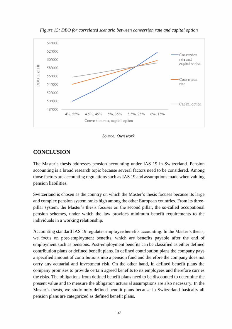
57
Figure 15: DBO for correlated scenario between conversion rate and capital option
Source: Own work.
CONCLUSION
The Master’s thesis addresses pension accounting under IAS 19 in Switzerland. Pension
accounting is a broad research topic because several factors need to be considered. Among
those factors are accounting regulations such as IAS 19 and assumptions made when valuing
pension liabilities.
Switzerland is chosen as the country on which the Master’s thesis focuses because its large
and complex pension system ranks high among the other European countries. From its three-
pillar system, the Master’s thesis focuses on the second pillar, the so-called occupational
pension schemes, under which the law provides minimum benefit requirements to the
individuals in a working relationship.
Accounting standard IAS 19 regulates employee benefits accounting. In the Master’s thesis,
we focus on post-employment benefits, which are benefits payable after the end of
employment such as pensions. Post-employment benefits can be classified as either defined
contribution plans or defined benefit plans. In defined contribution plans the company pays
a specified amount of contributions into a pension fund and therefore the company does not
carry any actuarial and investment risk. On the other hand, in defined benefit plans the
company promises to provide certain agreed benefits to its employees and therefore carries
the risks. The obligations from defined benefit plans need to be discounted to determine the
present value and to measure the obligation actuarial assumptions are also necessary. In the
Master’s thesis, we study only defined benefit plans because in Switzerland basically all
pension plans are categorized as defined benefit plans.

58
The value that represents the present value of benefits that a company promised its
employees is the DBO. In the statement of financial position, the net defined benefit
liability/asset must be recognized, which is the difference between the present value of the
DBO and the fair value of plan assets. This difference can either be a deficit if the present
value of the DBO is larger than the fair value of plan assets, or a surplus if the present value
of the DBO is smaller than the fair value of plan assets but adjusted by the asset ceiling. The
present value of the DBO must be determined using the PUC method, where each period of
service gives rise to an additional unit of benefit entitlement. The DBO can also change when
actuarial assumptions change, which can result in actuarial gains and losses. Actuarial gains
and losses can generally be categorized as gains or losses from demographic assumptions,
from financial assumptions, and from experience.
When a company promises to pay a certain amount of benefits to its employees, the timing
and duration of these benefits are not certain, therefore the actuary must make assumptions
about future events. They are a company’s best estimate of the variables that will determine
the ultimate cost of providing post-employment benefits. The actuarial assumptions are
divided into two categories: demographic assumptions and financial assumptions.
Demographic assumptions are important to determine when the promised benefits will be
paid and how the population is changing. To determine the life expectancy of employees the
company needs the mortality rate assumption, which is set by choosing a certain mortality
table and mortality improvement, which adds the assumption how the population will change
in the future. Companies can also provide special benefits, such as if the employee becomes
disabled or they leave the company, in which case the company needs to choose the disability
and turnover rate. These rates are usually included in the standard tables, but if the company
wants to adjust the rates to better represent the company’s rates, a fixed percentage, called a
loading factor, is applied to the standard tables. The company must also assess what
percentage of their employees will use the capital option at retirement. In Switzerland, the
conversion rate must be determined as well because the retirement savings are multiplied by
this rate.
Financial assumptions are important to project the number of benefits that the company
promised. The first financial assumption is the discount rate, which is used to determine the
present value of the DBO. The discount rate is set by reference to market yields at the end
of the reporting period on HQCB. The next financial assumption is the interest credit rate,
which is also used to determine the value of the DBO. The inflation rate assumption is used
to determine other financial assumptions. The salary increase rate is used to project an
employee’s future salary. The social security increase rate measures the annual expected
increase of the Swiss first pillar. Finally, the pension increase rate is used to project an
employee’s future pension.
The goal of the Master’s thesis is to perform a sensitivity analysis on the DBO on a test
dataset of policies for a typical Swiss pension plan. Since companies have some flexibility

59
when choosing parameter values of actuarial assumptions, the Master’s thesis’ results show
how different parameter values impact the DBO. Our research questions were:
How does the DBO change if we use a different parameter value for an actuarial
assumption?
Is the increase/decrease of the DBO in line with our expectations and predictions?
Which assumptions have the largest effect on the DBO?
For our sensitivity analysis we focused on how the following parameters impact the DBO:
conversion rate,
capital option,
loading factor on the turnover rate,
loading factor on the disability rate,
discount rate,
interest credit rate, and
salary increase rate.
For our baseline parameter values, we used the most common values that occur in the Swiss
market.
The benefit pension plan used is representative of a typical Swiss pension plan. Our test
dataset of policies is chosen to represent the Swiss working population by gender and the
Swiss overall population by age. The valuation tool used to perform the sensitivity analysis
calculated the DBO for our chosen feasible parameter values, pension plan, and dataset. The
valuation tool calculates the DBO as the sum of termination benefits, retirement benefits,
survivors’ benefits, and disability benefits over the ages 17-120.
The results of the sensitivity analysis reveal how the DBO changes. A 10bp
increase/decrease in the conversion rate may increase/decrease the DBO by 0.5%. A 10%
increase/decrease in the capital option may decrease/increase the DBO by 3.0%. A 10%
increase in the loading factor on the turnover rate may decrease the DBO by 1.1%, while a
10% decrease may increase the DBO by 1.5%. A 10% increase/decrease in the loading factor
on the disability rate may increase/decrease the DBO by 0.5%. A 10bp increase in the
discount rate may decrease the DBO by 1.8%, while a 10bp decrease may increase the DBO
by 2.1%. A 10bp increase/decrease in the interest credit rate may increase/decrease the DBO
by 0.6%. A 10bp increase/decrease in the salary increase rate may increase/decrease the
DBO by 0.3%.
The results are in line with our expectations and the biggest difference in the DBO is caused
by the change in the capital option parameter values, followed by the discount rate, and the
loading factor on the turnover rate. The effect on the DBO is the smallest when the salary

60
increases rate parameter value changes. However even the smallest change may have adverse
effects, but that effect can only be judged on a company to company basis.
As a final remark, we present a practical example of how the results of all the sensitivity
analyses can be used in practice and calculate three additional sensitivity analyses showing
the impact of correlated assumptions on the DBO.
As the world demographic is rapidly changing, pension accounting should reflect these
changes. Companies should as well be held accountable when choosing financial
assumptions, as these also reflect in pension accounting. To conclude, the Master’s thesis
contributes to a better understanding of how the DBO is affected by actuarial assumptions.
REFERENCE LIST
1. Ablebits. (n.d.). Ultimate Suits for Excel. Retrieved April 22, 2019, from
https://www.ablebits.com/excel-suite/index-2019.php
2. Adriatic Slovenica. (2019). Annual Report 2018. Koper: Adriatic Slovenica d. d.
3. Antolin, P., Schich, S. & Yermo, J. (2011). The Economic Impact of Protracted Low
Interest Rate on Pension Funds and Insurance Companies. OECD Journal: Financial
Markets Trends, 2011(1), 237−256.
4. AON Hewitt, Retirement and Investment. (2014). Society of Actuaries Finalizes New
Mortality Assumptions, The Financial and Strategic Implications for Pension Plan
sponsors. Aon plc.
5. Aon Switzerland Ltd., Retirement. (2017). Longevity Assumptions, alternative model for
projecting future mortality improvements in Switzerland. Zürich: Aon Switzerland Ltd.
6. AXA Insurance Ltd. (2017). A practical guide to occupational benefits. Winterthur:
AXA Insurance Ltd.
7. AXA Insurance Ltd. (2018). All you need to know about Pillar 2. Winterthur: AXA
Insurance Ltd.
8. AXA Insurance Ltd. (2019a). Pillar 1. Retrieved July 30, 2019, from AXA:
https://www.axa.ch/content/axa/en/vorsorge/1-saeule.html
9. AXA Insurance Ltd. (2019b). Pillar 2. Retrieved July 30, 2019, from AXA:
https://www.axa.ch/en/vorsorge/pillar-2.html
10. AXA Insurance Ltd. (2019c). Pillar 3. Retrieved July 30, 2019, from AXA:
https://www.axa.ch/content/axa/en/vorsorge/3-saeule.html
11. Bayerische Pensions Service GmbH. (n.d.). Pensionszusagen - Bewertungsverfahren.
Retrieved September 2, 2019, from http://www.bps-
online.bayern/assets/files/PDF/151007_Pensionszusagen_Bewertungsverfahren.pdf
12. Boulanger, F., Cossette, C. & Ouellet, G. (2007). Demographic and economic
assumptions used in actuarial valuations of social security and pension schemes.
Helsinki: International Social Security Association.

61
13. Brown, S. (2004). The Impact of Pension Assumptions on Firm Value. Atlanta: Emory
University.
14. Bui, T. & Randazzo, A. (2015). Why Discount Rates Should Reflect Liabilities: Best
Practices for Setting Public Sector Pension Fund Discount Rates. Reason Foundation.
15. Bundesamt für Sozialversicherungen BSV. (2018). Beträge gültig ab dem 1. Januar
2019. Bern: Schweizerische Eidgenossenschaft.
16. Bundesamt für Statistik. (2019). Social Security. Neuchatel: Federal Statistical Office.
17. Chand, J., & Jaeger, A. (1996). Aging Populations and Public Pension Schemes.
International Monetary Fund.
18. Continuous Mortality Investigation Limited. (2018). CMI_2017: the latest version of the
CMI Mortality Projections Model. London: Institute and faculty of Actuaries.
19. Corporate Finance Institute. (n.d.). What is Sensitivity Analysis? Retrieved May 11, 2019,
from https://corporatefinanceinstitute.com/resources/knowledge/modeling/what-is-
sensitivity-analysis/
20. Deloitte. (2010). IAS Plus Update. London: Deloitte Touche Tohmatsu.
21. Die Bundesversammlung der Schweizerischen Eidgenossenschaft. (2017, October 1).
Bundesgesetz über die Freizügigkeit in der beruflichen Alters-, Hinterlassenen- und
Invalidenvorsorge. Retrieved May 22, 2019, from
https://www.admin.ch/opc/de/classified-compilation/19930375/index.html
22. Die Bundesversammlung der Schweizerischen Eidgenossenschaft. (2019, January 1).
Bundesgesetz über die berufliche Alters-, Hinterlassenen- und Invalidenvorsorge.
Retrieved May 22, 2019, from https://www.admin.ch/opc/de/classified-
compilation/19820152/index.html
23. Eling, M. (2013). Intergenerational Transfers and the Stability of the Swiss Retirement
System. The Geneva Papers (38), 701−728.
24. European Actuarial Consultative Group. (2001). Actuarial Methods and Assumptions
used in the Valuation of Retirement Benefits in the EU and other European countries.
London: European Actuarial Consultative Group.
25. Fasshauer, J., & Glaum, M. (2009). Value Relevance of Level-3 Fair Values: The Case
of German Companies’ Pension Accounting Information. Giessen: University of
Giessen.
26. Federal Statistical Office. (2018a). Arbeitsmarktindikatoren 2018. Neuchatel: Federal
Statistical Office (FSO).
27. Federal Statistical Office. (2018b). Switzerland's population 2017. Neuchatel: Federal
Statistical Office.
28. Frees, E. (2003). Pension plan termination and retirement study. North American
Actuarial Journal, 9 (4).
29. Fried, A., Davis-Friday, P. & Davis, H. (2010). Accounting Choice, Economic
Environment and Employee Demographics. New York: Economic Environment and
employee demographics.

62
30. Fried, A., Davis-Friday, P. & Davis, H. (2014, October). The impact of duration on
management's discount rate choice. Research in Accounting Regulation, 26 (2),
217−221.
31. Gomes, B., Heeralall, S., Poli, F., & Sommer, R. (2017). Pension accounting - how it
developed over time. EFRAG.
32. Gorenje. (2019). Annual Report 2018. Velenje: Gorenje d. o. o.
33. Hayes, A. (2019, March 28). Stratified Random Sampling. Retrieved April 21, 2019,
from https://www.investopedia.com/terms/stratified_random_sampling.asp
34. IAS Plus. (n.d.). IAS 19 - Employee Benefits (2011). Retrieved March 1, 2019, from
https://www.iasplus.com/en/standards/ias/ias19
35. IFRS Staff paper. (2016, November 13). Present value measurement - discount rates
research. Retrieved March 1, 2019, from https://www.iasplus.com/en/meeting-
notes/ifrs-ic/not-added/2013/ias-19-discount-rate
36. International Accounting Standards Board. (2011). IAS 19 Employee Benefits. Retrieved
March 1, 2019, from http://eifrs.ifrs.org/eifrs/bnstandards/en/IAS19.pdf
37. Kasaoka, E. (2015). The Determinants of Discount Rates on Retirement Benefits in
Japan. International Review of Business, 15, 45−80.
38. KPMG. (2013). KPMG's Swiss Pensions Accounting Survey 2013. Zürich: KPMG.
39. KPMG. (2018). Swiss Pension Accounting Survey 2018; An analysis of market trends in
pension accounting. Zürich: KPMG AG.
40. Kuhn, M. (2019, August 1). IAS 19 in Switzerland - Senior Manager Interview. (M.
Pergar, Interviewer)
41. Libera AG, Aon Schweiz AG. (2014). Machbarkeitsstudie: Versicherungstechnische
Grundlagen für die berufliche Vorsorge. Zürich: Bundesamt für Statistik, Bundesamt für
Sozialversicherungen.
42. Libera AG, Aon Schweiz AG. (2015). Projekt BVG 2015. Retrieved May 8, 2019, from
http://www.bvg-grundlagen.ch/deutsch/projekt.htm
43. Mcbride, S. (2018, June 18). Danger Zone: Pension Accounting - Discount Rates.
Retrieved March 31, 2019, from https://www.newconstructs.com/danger-zone-pension-
accounting-discount-rates/
44. Mercer. (2018). Melbourne Mercer Global Pension Index. Melbourne: Australian Centre
for Financial Studies.
45. Napier, C. J. (2009). The Logic of Pension Accounting. International Accounting Policy
Forum, 231−249.
46. Nolfi, P. (1959). Die Berücksichtigung der Sterblichkeitsverbesserung in der
Rentenversicherung nach der Optimalmethode der Spieltheorie. Mitteilungen der
Vereinigung.
47. Obaidullah, J. (2018, June 9). Projected Benefit Obligation. Retrieved July 15, 2019,
from https://xplaind.com/888230/pension-accounting
48. OECD. (2014). Mortality Assumptions and Longevity Risk: Implications for pension
funds and annuity providers. Paris: OECD Publishing.

63
49. Oliver, M. (2009). Assessment and selection of actuarial assumptions for measuring
pension obligations. Society of Actuaries.
50. Perry, L. (2014, June 19). Auditing Special Purpose Frameworks: Materiality Levels.
Retrieved May 4, 2019, from https://www.accountingweb.com/aa/auditing/auditing-
special-purpose-frameworks-materiality-levels
51. Plamondon, P., Drouin, A., Binet, G., Cichon, M., McGillivray, W. R., Bédard, M. &
Perez-Montas, H. (2002). Actuarial practice in social security. Geneva: International
Labour Office/International Social Security Association.
52. Punter Southall Briefing Note. (2010). The impact of deflation on pensions. London:
Punter Southall Group.
53. Ruppel, W. (2017). Wiley GAAP for Governments 2017 ‐ Interpretation and Application
of Generally Accepted Accounting Principles for State and Local Governments. John
Wiley & Sons, Ltd.
54. Schweizerische Bundeskanzlei. (n.d.a). Early withdrawal of pension funds. Retrieved
July 17, 2019, from Swiss authorities online: https://www.ch.ch/en/withdraw-pension-
early/
55. Schweizerische Eidgenossenschaft. (2018). Bundesverfassung der Schweizerischen
Eidgenossenschaft. Bern: Schweizerische Eidgenossenschaft.
56. Schweizerische Kammer der Pensionskassen-Experten. (2019, March 31).
Internationale Rechnungslegung. Retrieved May 11, 2019, from
http://skpe.ch/de/themen/internationale-rechnungslegung.html
57. Swiss Confederation. (2018). Federal Constitution of the Swiss Confederation. Bern:
Swiss Confederation.
58. Swiss National Bank. (2019, March 21). SNB conditional inflation forecast. Retrieved
April 7, 2019, from https://data.snb.ch/en/topics/snb#!/cube/snbiproga
59. Swissstaffing. (2019). Interest yield. Retrieved August 5, 2019, from
https://www.swissstaffing-bvg.ch/en/key_data_investments/interest_yield.php
60. The Economist. (2014, August 23). My money or your life. Retrieved March 1, 2019,
from https://www.economist.com/finance-and-economics/2014/08/23/my-money-or-
your-life
61. UBS AG. (2019, February 11). Pension or lump-sum payment? Retrieved April 7, 2019,
from https://www.ubs.com/ch/en/private/pension/information/magazine/2019/pension-
or-lumpsum-payment.html
62. UK Government. (2017, July 13). Chapter 1: life expectancy and healthy life expectancy.
Retrieved March 3, 2019, from https://www.gov.uk/government/publications/health-
profile-for-england/chapter-1-life-expectancy-and-healthy-life-expectancy
63. UniCredit Banka Slovenija. (2019). 2018 Annual Report. Ljubljana: UniCredit Banka
Slovenija d. d.
64. Vermögens Zentrum. (n.d.). Der Umwandlungssatz bestimmt die Rente. Retrieved April
18, 2019, from
https://www.vermoegenszentrum.ch/ratgeber/wissensbeitrage/privatkunden/pensionieru
ng-planen/der-umwandlungssatz-bestimmt-die-rente.html

64
65. Willis Towers Watson. (2010, October). Actuarial assumptions. Retrieved March 2,
2019, from https://www.towerswatson.com/en-IN/Insights/IC-Types/Technical-
Regulatory/2010/Actuarial-assumptions
66. Willis Towers Watson. (2018, August 1). 2018 Global Survey of Accounting
Assumptions for Defined Benefit Plans: Executive Summary. Retrieved May 12, 2019,
from
https://webcache.googleusercontent.com/search?q=cache:7YglyZNJwnAJ:https://www
.willistowerswatson.com/en/insights/2018/07/2018-accounting-assumptions-survey-
for-defined-benefit-plans+&cd=17&hl=sl&ct=clnk&gl=uk
67. Zavarovalnica Sava. (2019). Letno poročilo Zavarovalnice Sava 2018. Maribor:
Zavarovalnica Sava d. d.
68. Zavarovalnica Triglav. (2019). The Triglav Group and Zavarovalnica Triglav d.d.
Annual Report 2018. Ljubljana: Triglav Group and Zavarovalnica Triglav d. d.
69. ZPIZ-2. (2018). Zakon o pokojninskem in invalidskem zavarovanje (ZPIZ-2). Uradni list
Republike Slovenije.
70. Zurich Insurance Company Ltd. (2019). Deferred retirement. Retrieved August 3, 2019,
from https://www.vita.ch/en/services/reporting-your-retirement/deferred-retirement

APPENDIXES


1
Appendix 1: Povzetek (Summary in the Slovene language)
Magistrsko delo proučuje mednarodni računovodski standard 19, ki ureja zaslužke
zaposlencev. V delu sem se osredotočila na pozaposlitvene zaslužke, kar so prejemki po
koncu zaposlitve, kot so na primer pokojnine. Pozaposlitveni zaslužki se lahko razvrstijo kot
programi z določenimi prispevki ali kot programi z določenimi zaslužki. V programih z
določenimi prispevki podjetje vplača določen znesek v pokojninski sklad in zato ni
izpostavljeno aktuarskemu in naložbenemu tveganju. Po drugi strani pa podjetje v programih
z določenimi zaslužki obljubi, da bo zagotovilo dogovorjene zaslužke za svoje zaposlene in
tako nosi aktuarsko in naložbeno tveganje. Obveznosti za programe z določenimi zaslužki
je treba diskontirati za določitev sedanje vrednosti in za merjenje obveznosti so potrebne
tudi aktuarske predpostavke. V magistrskem delu torej proučujem samo programe z
določenimi zaslužki, ker delodajalec nosi tveganja in ker so v Švici praktično vsi pokojninski
načrti programi z določenimi zaslužki. Podjetja, ki svojim zaposlenim obljubljajo določene
zaslužke, morajo upoštevati, kakšna bo sedanja vrednost teh prihodnjih zaslužkov. Ta
vrednost se imenuje tudi obveznost za določene zaslužke.
Magistrsko delo se osredotoča na Švico, saj se njen pokojninski sistem uvršča visoko med
drugimi evropskimi državami. Njen pokojninski sistem sestavljajo trije stebri, vendar se v
delu osredotočim samo na drugi steber, kjer zakon določuje minimalne pogoje za ljudi v
službenem razmerju.
Kadar podjetje obljubi, da bo zaposlenim zagotovilo določene zaslužke, čas in trajanje
izplačila teh zaslužkov nista znana, zato mora aktuar določiti predpostavke o gibanju
prihodnih denarnih tokov. Te predpostavke predstavljajo najboljšo oceno spremenljivk, ki
bodo določile končne stroške zagotavljanja pozaposlitvenih zaslužkov. Aktuarske
predpostavke so razdeljene v dve kategoriji: demografske predpostavke in finančne
predpostavke.
Demografske spremembe predstavljajo velik izziv za vse razvite države, zlasti kar zadeva
njihove pokojninske sisteme. S staranjem prebivalstva bo treba pokojnine izplačevati za
daljša obdobja. To vpliva na podjetja, saj so svojim zaposlenim obljubila pozaposlitvene
zaslužke. Če ne upoštevajo demografskih sprememb, lahko podcenijo količino zaslužkov, ki
jih bodo morali zagotoviti v prihodnosti. Demografske predpostavke so pomembne za
določitev, kdaj bodo obljubljeni zaslužki izplačani in kako se prebivalstvo spreminja. Za
določitev pričakovane življenjske dobe zaposlenih potrebuje podjetje predpostavko o stopnji
umrljivosti, ki je določena z izbiro tablice umrljivosti in izboljšavo smrtnosti, ki pove, kako
se bo prebivalstvo v prihodnje spreminjalo. Podjetja lahko zagotavljajo tudi posebne
zaslužke, na primer, če postane delavec invalid ali zapusti podjetje. V tem primeru mora
podjetje izbrati stopnjo invalidnosti in stopnjo fluktuacije. Podjetje mora oceniti tudi,
kolikšen odstotek zaposlenih bo pokojnino prevzel v enem znesku, kar se imenuje kapitalska
opcija. V Švici je treba določiti tudi menjalno stopnjo, saj se pokojninski prihranki
pomnožijo s to vrednostjo.

2
Pokojnine so prav tako odvisne od finančnih predpostavk, kot so diskontna stopnja, inflacija,
povišanja plač in druge. Podjetja morajo ustrezno izbrati te predpostavke za vrednotenje
njihovih obveznosti za določene zaslužke. Na primer, če je diskontna stopnja previsoka, se
podjetju zmanjša obveznost. Ustrezna izbira predpostavk je zaradi tega pomembna.
Finančne predpostavke so pomembne za ocenitev zaslužkov, ki jih je podjetje obljubilo. Prva
finančna predpostavka je diskontna stopnja, ki se uporablja za določitev sedanje vrednosti
obveznosti za določene zaslužke. Naslednja finančna predpostavka je obrestna mera, ki se
prav tako uporablja za določitev sedanje vrednosti obveznosti za določene zaslužke.
Predpostavka o stopnji inflacije se uporablja pri določanju vrednosti drugih finančnih
predpostavk. Stopnja rasti plač se uporablja za ocenitev prihodnje plače zaposlenega.
Stopnja povečanja socialne varnosti meri letno pričakovano povečanje švicarskega prvega
stebra. Nazadnje, stopnja povečanja pokojnine se uporablja za ocenitev prihodnje pokojnine
zaposlenega.
Namen magistrskega dela je proučiti, kako se obveznosti za določene zaslužke spremenijo,
ko se spremeni ena demografska ali finančna predpostavka. Cilj magistrskega dela je izvesti
analizo občutljivosti na obveznostih za določene zaslužke na testnem vzorcu polic za tipični
švicarski pokojninski načrt. Analiza občutljivosti v pričujočem delu vedno temelji na
spremembi samo ene aktuarske predpostavke, za ostale predpostavke pa predpostavi, da so
konstante. Rezultati analize občutljivosti pokažejo, kako velik je lahko učinek na obveznosti
za določene zaslužke, če se ena predpostavka spremeni. Cilj magistrskega dela ni odgovoriti
na vprašanje, ali je učinek na obveznosti dober ali slab, ugotoviti poskušamo samo, za koliko
odstotkov se obveznost lahko spremeni.
Raziskovalna metodologija obsega teoretični in empirični del. Teoretični del je sestavljen iz
treh poglavij. Prvo poglavje opisuje mednarodni računovodski standard 19 in obveznosti za
določene zaslužke. Drugo poglavje opiše švicarski pokojninski sistem. Tretje poglavje se
nanaša na aktuarske predpostavke. Ta del služi kot osnova za razumevanje empiričnega dela.
Empirični del je sestavljen iz dveh poglavij. V prvem poglavju sem opisala, katere
predpostavke sem vključila v analizo, podrobnosti švicarskega pokojninskega načrta, ki je
bil uporabljen, kako je bil izbran testen vzorec podatkov in kako deluje orodje za izračun
obveznosti za določene zaslužke ter kako smo ga prilagodili našim podatkom. V drugem
poglavju predstavim rezultate iz analize občutljivosti in opišem, kakšen vpliv ima vsaka
predpostavka, na koncu pa naredim tri dodatne analize, ko so spremenljivke povezane.
Rezultati iz empiričnega dela odgovarjajo na naslednja vprašanja:
Kako se obveznost za določene zaslužke spremeni, če spremenimo eno aktuarsko
predpostavko?
Ali je povečanje/zmanjšanje obveznosti za določene zaslužke v skladu z našimi
pričakovanji?
Katere predpostavke imajo največji učinek na obveznosti za določene zaslužke?

3
Kako se spreminjajo obveznosti za določene zaslužke, je opisano v nadaljevanju.
Povečanje/zmanjšanje menjalne stopnje za 10 bazičnih točk lahko poveča/zmanjša
obveznosti za določene zaslužke za 0,5 %. 10-odstotno povečanje/zmanjšanje kapitalske
opcije lahko zmanjša/poveča obveznosti za določene zaslužke za 3,0 %. 10-odstotno
povečanje faktorja na stopnjo fluktuacije lahko zmanjša obveznosti za določene zaslužke za
1,1 %, 10-odstotno zmanjšanje pa lahko poveča obveznosti za določene zaslužke za 1,5 %.
10-odstotno povečanje/zmanjšanje faktorja na stopnjo invalidnosti lahko poveča/zmanjša
obveznosti za določene zaslužke za 0,5 %. Zvišanje diskontne stopnje za 10 bazičnih točk
lahko zmanjša obveznosti za določene zaslužke za 1,8 %, zmanjšanje za 10 bazičnih točk pa
lahko poveča obveznosti za določene zaslužke za 2,1 %. Povečanje/znižanje obrestne mere
za 10 bazičnih točk lahko poveča/zmanjša obveznosti za določene zaslužke za 0,6 %.
Povečanje/zmanjšanje stopnje rasti plač za 10 bazičnih točk lahko poveča/zmanjša
obveznosti za določene zaslužke za 0,3 %.
Rezultati so v skladu z našimi pričakovanji in največja razlika v obveznostih za določene
zaslužke je posledica spremembe predpostavke kapitalske opcije, ki ji sledita predpostavka
o diskontni stopnji in faktor na stopnjo fluktuacije. Učinek na obveznosti za določene
zaslužke je najmanjši pri predpostavki o stopnji rasti plač. Toda tudi najmanjša sprememba
ima lahko materialne posledice, vendar se morajo te posledice določiti za vsako podjetje
posebej.
Ker se svetovna populacija hitro spreminja, se morajo te spremembe odražati pri izračunu
pokojnin. Prav tako morajo biti podjetja odgovorna tudi pri izbiri finančnih predpostavk, saj
se tudi te predpostavke odrazijo pri računovodenju. Za zaključek, magistrsko delo prispeva
k boljšemu razumevanju, kako aktuarske predpostavke vplivajo na obveznosti za določene
zaslužke.

4
Appendix 2: Sensitivity analyses results
Table 17: Conversion rate sensitivity analysis results
Conversion rate DBO in kCHF Change in DBO
5.0% 56,860 -2.6%
5.5% 58,370 0.0%
6.0% 59,879 2.6%
6.5% 61,388 5.2%
6.8% 62,293 6.7%
Source: Own work.
Table 18: Capital option sensitivity analysis results
Capital option DBO in kCHF Change in DBO
0% 62,714 7.4%
10% 60,976 4.5%
25% 58,370 0.0%
50% 54,025 -7.4%
100% 45,337 -22.3%
Source: Own work.
Table 19: Loading factor on turnover rate sensitivity analysis results
Loading factor on
the turnover rate DBO in kCHF Change in DBO
50% 62,848 7.7%
75% 60,411 3.5%
100% 58,370 0.0%
150% 55,156 -5.5%
200% 52,753 -9.6%
Source: Own work.
Table 20: Loading factor on disability rate sensitivity analysis results
Loading factor on
disability rate DBO in kCHF Change in DBO
80% 57,758 -1.0%
table continues

5
Table 20: Loading factor on disability rate sensitivity analysis results (cont.)
85% 57,911 -0.8%
90% 58,064 -0.5%
100% 58,370 0.0%
125% 59,128 1.3%
Source: Own work.
Table 21: Discount rate sensitivity analysis results
Discount rate DBO in kCHF Change in DBO
-0.48% 70,817 21.3%
0.02% 64,077 9.8%
0.27% 61,106 4.7%
0.42% 59,438 1.8%
0.52% 58,370 0.0%
0.62% 57,335 -1.8%
0.77% 55,845 -4.3%
1.02% 53,514 -8.3%
1.52% 49,363 -15.4%
Source: Own work.
Table 22: Interest credit rate sensitivity analysis results
Interest credit
rate DBO in kCHF Change in DBO
0.5% 56,708 -2.8%
1.0% 58,370 0.0%
1.5% 60,079 2.9%
2.0% 61,836 5.9%
2.5% 63,673 9.1%
Source: Own work.
Table 23: Salary increase rate sensitivity analysis results
Salary increase
rate DBO in kCHF Change in DBO
table continues

6
Table 23: Salary increase rate sensitivity analysis results (cont.)
0.0% 56,175 -3.8%
0.5% 57,441 -1.6%
1.0% 58,370 0.0%
2.0% 60,125 3.0%
3.0% 61,920 6.1%
Source: Own work.
Table 24: Discount rate and conversion rate correlation sensitivity analysis results
Discount rate Conversion
rate DBO in kCHF
Change in
DBO
-0.48% 4.50% 66,870 14.6%
0.02% 5.00% 62,355 6.8%
0.27% 5.25% 60,301 3.3%
0.42% 5.40% 59,128 1.3%
0.52% 5.50% 58,370 0.0%
0.62% 5.60% 57,630 -1.3%
0.77% 5.75% 56,553 -3.1%
1.02% 6.00% 54,843 -6.0%
1.52% 6.50% 51,714 -11.4%
Source: Own work.
Table 25: Discount rate, conversion rate, and interest credit rate correlation sensitivity
analysis results
Discount rate Conversion
rate
Interest
credit rate
DBO in
kCHF
Change in
DBO
-0.48% 4.50% 0.00% 63,592 8.9%
0.02% 5.00% 0.50% 60,776 4.1%
0.27% 5.25% 0.75% 59,521 2.0%
0.42% 5.40% 0.90% 58,819 0.8%
0.52% 5.50% 1.00% 58,370 0.0%
0.62% 5.60% 1.10% 57,933 -0.7%
0.77% 5.75% 1.25% 57,302 -1.8%
1.02% 6.00% 1.50% 56,300 -3.5%
1.52% 6.50% 2.00% 54,493 -6.6%
Source: Own work.

7
Table 26: Conversion rate and capital option correlation sensitivity analysis results
Conversion
rate Capital option DBO in kCHF
Change in
DBO
4.00% 55.00% 49,927 -14.5%
4.50% 45.00% 52,453 -10.1%
5.00% 35.00% 55,267 -5.3%
5.50% 25.00% 58,370 0.0%
6.00% 15.00% 61,761 5.8%
Source: Own work.