Three dimensional digital analysis of 2,500 square kilometers of gravity and magnetic

survey data, Bellefontaine Outlier area, Ohio.

A Senior Thesis

Submitted as Partial Fulfillment of the Requirements

for the degree Bachelor of Science in

Geological Sciences at

The Ohio State University

by

Michael L. Fidler Jr.

The Ohio State University, Spring Quarter 2003.

_________________________________

Dr. Hallan C. Noltimier

Acknowlegements

I would like to offer a heartfelt thanks to everyone who has helped with this project,

especially Dr. Noltimier, my thesis adviser, who has been instrumental in my entire academic

career. He has offered encouragement and guidance at every step of my extended course of study.

I would like to thank Jacinda Nettik and the rest of the staff at Rockware for granting me a user

license for RockWorks2002©. To my family who has been very patient and supportive all these

years, and, to the friends who have helped me with this project by providing their unending

support, opinions, and much needed technical assistance, Thank You All.

ii

Table of Contents

Title Page........................................................................................................i

Acknowlegements..........................................................................................ii

Index of figures.............................................................................................iv

Index of tables................................................................................................v

Part 1: Introduction..................................................................................... 1

Part 2: Background Geological Information............................................... 5

Part 3: Methods and proof of concept....................................................... .11

Part 4: Basement Model from gravity data................................................ 13

part 5. Basement Model from Geomagnetic data...................................... 19

part 6: Conclusions.................................................................................... 25

References....................................................................................................26

Appendix: Summery of data points and gradient measurements...............28

iii

Index of figures

1. Map of Ohio showing lithologic provinces, the Bellefontaine Outlier, and the location of thesurvey area. From Weaver (1994) .....................................................................................................1

2. Reprocessed COCORP seismic image within the Outlier area showing high angle faults. FromWeaver (1994) ....................................................................................................................................2

3. Field station locations (510) of Weaver's gravity and magnetic survey. From Weaver(1994).......34. Distribution of known faults in the survey area and surrounding region. Modified after

Wickstrom (1990), from Weaver (1994). .........................................................................................45. Stratigraphic column of the Precambrian-Ordovician in Ohio. From Hansen (1998) ....................66. Stratigraphic column of survey region from the Precambrian Middle Run Formation to the

Silurian/Devonian. Adapted from Paramo (2002) ............................................................................77. General model of Precambrian structure in ohio and the neighboring states. Modified from

Hansen, (1997) ....................................................................................................................................98. Suggested extension of the MCR into southwest Ohio. ..................................................................109. Contour graph of artifact field simulating a simple vertical displacement (SVD). ........................1110.Three dimensional graph of the slope of the artifact field simulating a simple vertical

displacement. .................................................................................................................1211.Contour graph of gravitational field with lines of maximum gradient in white. Field Contoured in

milligals with regional average survey field normalized to 0 milligals. .........................................1312.Contour graph of the slope of the gravitational field in degrees.....................................................1413.3D graph of the slopes (gradients) of the CBRA dataset ................................................................1514.Histogram of the calculated slopes of the graph of the gravitational field. ....................................1615.View of model of crystalline basement from CBRA dataset looking North. including Paleozoic

sedimentary rocks and surface topography. ....................................................................................1816.Contour graph of geomagnetic field (300 γ filtered) dataset with lines of maximum gradient in

white. Field contoured in gammas with regional average survey field normalized to 0 gamma. ..1917.Contour graph of the slope of the 300 γ filtered geomagnetic field dataset. ..................................2018.3D graph of the slopes (gradients) of the geomagnetic 300 γ filtered dataset. ..............................2119.Histogram of the calculated slopes of the graph of the geomagnetic (300 γ filtered) dataset. ......2220.View of model of crystalline basement from geomagnetic (300 γ filtered) dataset looking North,

including Paleozoic sedimentary rocks and surface topography. ...................................................24

iv

Index of Tables

Table 1) Fault throw calculations from gravity. Z0/Z1 in Km. ............................................................17

Table 2) Fault throw calculations from geomagnetic 300 γ filtered dataset. Δh in km. .....................23

v

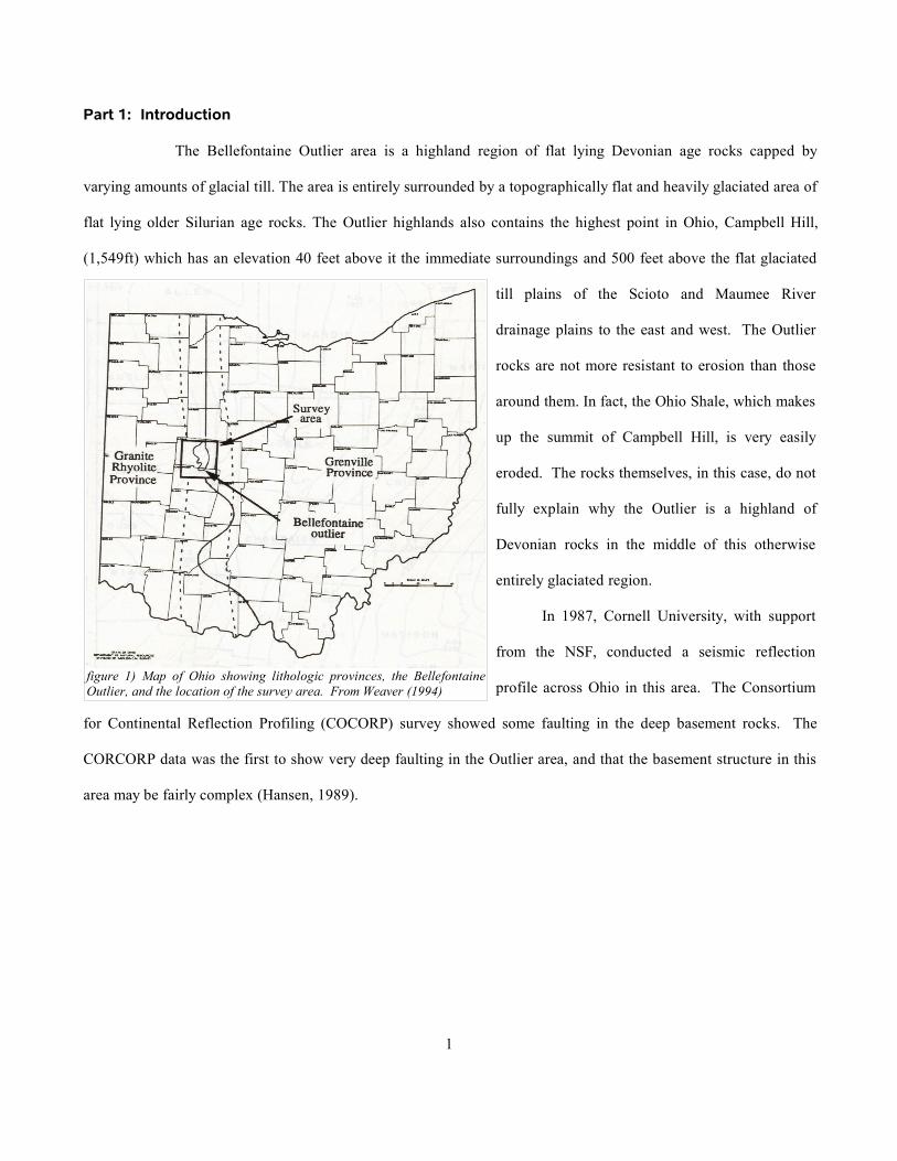
Part 1: Introduction

The Bellefontaine Outlier area is a highland region of flat lying Devonian age rocks capped by

varying amounts of glacial till. The area is entirely surrounded by a topographically flat and heavily glaciated area of

flat lying older Silurian age rocks. The Outlier highlands also contains the highest point in Ohio, Campbell Hill,

(1,549ft) which has an elevation 40 feet above it the immediate surroundings and 500 feet above the flat glaciated

till plains of the Scioto and Maumee River

drainage plains to the east and west. The Outlier

rocks are not more resistant to erosion than those

around them. In fact, the Ohio Shale, which makes

up the summit of Campbell Hill, is very easily

eroded. The rocks themselves, in this case, do not

fully explain why the Outlier is a highland of

Devonian rocks in the middle of this otherwise

entirely glaciated region.

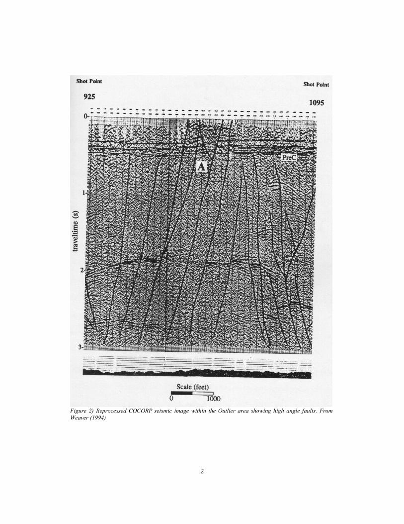
In 1987, Cornell University, with support

from the NSF, conducted a seismic reflection

profile across Ohio in this area. The Consortium

for Continental Reflection Profiling (COCORP) survey showed some faulting in the deep basement rocks. The

CORCORP data was the first to show very deep faulting in the Outlier area, and that the basement structure in this

area may be fairly complex (Hansen, 1989).

1

figure 1) Map of Ohio showing lithologic provinces, the BellefontaineOutlier, and the location of the survey area. From Weaver (1994)

2

Figure 2) Reprocessed COCORP seismic image within the Outlier area showing high angle faults. FromWeaver (1994)

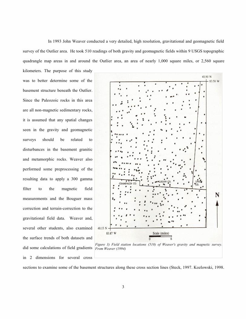
In 1993 John Weaver conducted a very detailed, high resolution, gravitational and geomagnetic field

survey of the Outlier area. He took 510 readings of both gravity and geomagnetic fields within 9 USGS topographic

quadrangle map areas in and around the Outlier area, an area of nearly 1,000 square miles, or 2,560 square

kilometers. The purpose of this study

was to better determine some of the

basement structure beneath the Outlier.

Since the Paleozoic rocks in this area

are all non-magnetic sedimentary rocks,

it is assumed that any spatial changes

seen in the gravity and geomagnetic

surveys should be related to

disturbances in the basement granitic

and metamorphic rocks. Weaver also

performed some preprocessing of the

resulting data to apply a 300 gamma

filter to the magnetic field

measurements and the Bouguer mass

correction and terrain-correction to the

gravitational field data. Weaver and,

several other students, also examined

the surface trends of both datasets and

did some calculations of field gradients

in 2 dimensions for several cross

sections to examine some of the basement structures along these cross section lines (Steck, 1997. Kozlowski, 1998.

3

Figure 3) Field station locations (510) of Weaver's gravity and magnetic survey.From Weaver (1994)

Kaltenbach, 1998). One of these cross sections was done to compare the gravity and magnetic cross sections with

the findings of the COCORP reflection survey line which crosses the northern third of the survey area (Weaver,

1994).

This study utilizes Weaver's gravity and magnetic survey and, instead of looking at discrete cross

sections, holistically examines the entire dataset to better analyze the data from the survey using modern

computational tools. The field gradient at each grid point of the gridded data set was determined. Then the field

gradients were statistically examined to determine points of unusually high gradient and therefore short spacial

changes in the elevation of the basement structure. Many very short cross sections were then computed across

sections of statistically determined areas of basement structure. These cross sections were then used to build

approximate models of the entire Outlier area in 3 dimensions.

4

Figure 4) Distribution of known faults in the survey area and surrounding region. Modified afterWickstrom (1990), from Weaver (1994)

Part 2: Background Geological Information.

Precambrian geology.

The survey area for this study is at the western edge of the Grenville Front Tectonic Zone. The

Grenville Orogeny occurred 900 Ma to 1.0 Ga B.P. and is the result of a Proterozoic plate collision. The location of

the boundary between the Grenville Province and the Granite-Rhyolite Province is not well mapped, but has been

determined approximately by seismic studies such as the COCORP survey across Ohio. To the west of this

boundary, the basement rocks are Granite-Rhyolite Province rocks, mostly cratonic granite and rhyolite dated

radiometrically to approximately 1480 Ma B.P. To the east of this boundary, the Grenville Province rocks form the

deep basement structure. These rocks are predominately amphibolite faces igneous, metamorphic igneous and

metamorphic sedimentary rocks dated to approximately 880 to 1100 Ma B.P. These rocks are denser than the

Paleozoic Bedrock, and have a magnetic susceptibility much greater than the sedimentary strata overlying them in

the survey area and will be the controlling influence on any spatial magnetic or gravitational field changes in this

study (Weaver, 1994).

The depth to this dense crystalline basement has been determined by recent seismic studies nearby to

the north in Allen County to be approximately 5700 m deep (Paramo, 2002). Since the dominant trends of this layer

are topographically changing in an East-West orientation, the depth to the north should be a good approximation of

the depth of the basement in our survey area as well (Weaver, 1994).

Overlying the crystalline basement rocks is a layer known as the Middle Run Formation, a lithic

arenite, and pink arkose sandstone with interbedded volcanic ash and siltstones that predates the Laurentia-

Grenville plate collision. The Middle Run was first identified by the ODNR Warren County Deep Core Well in

Warren County, Ohio. The ODNR well drilled and cored more than 2000 feet into this Precambrian sedimentary

rock (Hansen, 1989). The well core and seismic study of the area around the well showed the possibility of a large

half-graben structure filled in with this lithic arenite. It is possible that this structure represents an extension south

into Ohio of the Midcontinent Rift System (MCR), a pre-Grenville age structure which extends from Kansas into

Southern Michigan (Weaver, 1994).

5

Paleozoic geology.

Overlaying the unconformity that marks

the upper boundary of the Precambrian is the Mt. Simon

Sandstone. This is silica sandstone with silica cement,

possibly a beach sand thought to originate from a shelf-

type environment (Weaver, 1994). In Ohio this unit

grades upward to a conglomeritic sandstone. The

thickness in the survey area (from the Allerton

Resources Well #1) is about 120 feet with a mean

density of 2.42g/cc (Weaver, 1994).

The Mt Simon Sandstone is overlain by the Rome Formation which intertongues with the Eau Claire

Formation. In this region the Rome Formation has a thickness of 200 feet and a mean density of 2.60g/cc. The Eau

Claire Formation is a glauconitic siltstone, with layers of glauconitic shale common in the upper parts of the

formation (Weaver, 1994).

Overlaying the Eau Claire is the Kerbel Formation. In places it is overlain by the Conasauga

Formation where the Kerbel Formation is not present. The Kerbel Formation is nonglauconitic sandstone thought to

represent the change from marine to nonmarine delta deposition. The Kerbel Sandstone grades to a medium coarse

texture and becomes dolomitic in the upper part of the formation, which increases the overall density. The average

density is 2.79g/cc and in this area, thickness is 40 feet (Weaver, 1994).

6

Figure 5) Stratigraphic column of the Precambrian-Ordovicianin Ohio. From Hansen (1998)

The Knox Dolomite overlies the Kerbel Formation and

marks the boundary in this area of the Late Cambrian or

Ordovician period in the survey area. Of somewhat higher

density than the underlying sandstones, the Knox is a

microcrystalline Dolomite with a mean density of 2.84g/cc

and a thickness of 394 feet (as observed at national

Petroleum Well#1) (Weaver, 1994).

Following the deposition of the Knox Dolomite, there

was a regressive phase which created an unconformity at the

top of the unit. Overlying this unconformity are the thin

shales and siltstones of the Wells Creek Formation

(2.81g/cc), and overlying that, 480 feet thickness of the

Black River Limestone, a microcrystalline limestone with a

mean density of 2.79g/cc (Weaver, 1994).

The Black River Limestone is overlain by the Trenton Limestone, a fossiliferous, light gray to brown

limestone with black-shale partings. The unit increases in density towards the top of the unit's 310 feet of thickness.

It has a mean density of 2.64g/cc (Weaver, 1994).

The top of the Trenton Limestone becomes increasingly fossiliferous with more pyrite marking the

base of (what the Ohio Division of Geological Survey has recommended calling) the Undifferentiated Cincinnatian

Series. This is a layer of green shale with thin interlayered limestone, a thickness of 634 feet, with a uniform density

of 2.73g/cc (Weaver, 1994).

Overlaying the Undifferentiated Cincinnatian Series is 28 feet of the Whitewater Formation, a brown

medium crystalline limestone with a mean density of 2.73g/cc. The formation grades upward into a green shale

(Weaver, 1994).

The beginning of the Silurian Period is marked in this area by the bottom of the Brassfield Formation.

7

Figure 6) Stratigraphic column of survey region from thePrecambrian Middle Run Formation to theSilurian/Devonian. Adapted from Paramo (2002)

The Ordovician Whitewater Formation grades upward into a dolomitic green shale of the lower Brassfield, which

continues to grade upward into an argillaceous green dolomite. The boundary between the Ordovician and the

Silurian is not clearly defined in the survey area, but is in the region of green shale between these two rock layers.

The Brassfield Formation has a mean density of 2.83g/cc and a thickness of 107 feet in the survey area (Weaver,

1994).

The dolomite of the upper Brassfield Formation is overlain by a cherty limestone with interbedded

shale known as the Sub-Lockport Group. This layer is 34 feet thick and has a density of 2.82g/cc. The Sub-

Lockport Group grades up into the Lockport Dolomite. This is a light colored crystalline dolomite with a vuggy

porosity and stylolites. It has a mean density of 2.8g/cc and a thickness of 97 feet in this area (Weaver, 1994).

In this part of Ohio the Lockport Dolomite is overlain by the Greenfield Dolomite. The contact is

gradational. The Greenfield Dolomite has a mean density of 2.82g/cc and a local thickness of 47 feet (Weaver,

1994).

On top of the Greenfield Formation is the Tymochetee Dolomite. This is a argillaceous, and silty

dolomite with a mean density of 2.82g/cc and a local thickness of 70 feet (Weaver, 1994).

In the survey area, the Salina Group overlies the Tymochetee Dolomite. The Salina Group is a

generally gray, fine-crystalline dolomite with a mean density of 2.78g/cc and a thickness of 136 feet. The upper part

of this layer is a thinly laminated dolomitic shale (Weaver, 1994).

The base of the Columbus Limestone is, in this region, the boundary between the Silurian and the

Devonian Periods. This is a light colored fine-medium crystalline dolomite with chert, silt, and fossils. At its base

is a thin layer of fine grained well rounded sand. This layer has an average density of 2.69g/cc and a thickness in

the survey area of 87 feet (Weaver, 1994).

The Ohio Shale directly overlays the Columbus Limestone because the Delaware Limestone is absent

in this area. This is a very dark silty, pyritic, petroliferous, and siliceous shale with a mean density of 2.67g/cc and

a local thickness of 105 feet. This shale exhibits a high gamma-ray activity, and is thought to have been formed

from Catskill Delta deposits from the Eastern Appalachian region (Weaver, 1994).

8

Uplift of the continent during the Mesozoic and Cenozoic has prevented any Mesozoic to Tertiary

age sediments from being deposited in this area, but the survey area has undergone several phases of glaciation

during the Pleistocene. Pre-Illinoian, Illinoian, and two phases of the Wisconsinan stage are represented in the

Outlier area. A mean density for the total drift has been estimated to be 2.0g/cc. The thickness of this material over

the Outlier area ranges from 0 to 150 feet. In the late Wisconsinan glaciation, the advancing ice sheet was split into

two lobes by the Outlier highland (Weaver, 1994).

Tectonic history

The Grenville Tectonic Zone, the boundary of which lies in the survey area, is a zone of thrust

faulting resulting from a continental collision approximately 1.0 Ga B.P. This continental collision created

westward compression and overthrusting which has been interpreted from the COCORP survey seismic data, which

mapped an eastward dip to the sheared layers at depth which suggests that basement shear zones are directly over

the footwall ramp of the thrusts. The Appalachian Taconic Orogeny was the next major event in the region during

the late Ordovician Period. This Orogeny occurred as the Piedmont Terrane was added to the ancestral North

American continent by collision. High angle faults activated or reactivated by this event have been observed in the

outlier area by the COCORP survey. The Midcontinent Rift System is a Proterozoic rift system identified by gravity

9

Figure 7) General model of Precambrian structure in ohio and the neighboring states. Modified from Hansen, (1997)

and magnetic anomalies traced from Kansas north into Michigan (Figure 8). This rift system, which was likely

closed by the Grenville Orogeny compression, may run in a north-south trend through the survey area (Weaver,

1994).

10

Figure 8) Suggested extension of the MCR into southwest Ohio.

Shaded areas show trend of MCR. From Weaver (1994)

Part 3: Methods and proof of concept.

The method and Rockware© software that I used to analyze Weaver's gravity and magnetic datasets

was tested by generating an artificial dataset consisting of a single linear feature with a field change of the same

approximate magnitude found in the actual data. The artificial dataset used Weaver's original control points and

substituted invented field readings to approximate the same level of field change and resolution of the original

dataset but with a flat field and a single very simple linear feature that approximates a north/south trending high

angle fault. The computational steps later used to analyze the real data were executed against this dataset to the

point of the statistical determination of the position of the structure in two dimensions (Latitude and Longitude). It

11

Figure 9) Contour graph of artifact field simulating a simple vertical displacement (SVD).

was found that the process did statistically determine the position of the field change within the theoretical

maximum resolution of the survey.

First, the test dataset was gridded and normalized so that the maximum field change is the same size

as the total horizontal size to make slope analysis easier. A slope analysis was executed against the resulting gridded

normalized data. The slope analysis shows the slope of the contour graph of the data in degrees. The points of

maximum slope were connected by the white line shown in on the contour graph of the test data (Figure 9).

12

Figure 10) three dimensional graph of the slope of the artifact field simulating a simple vertical displacement.

Part 4: Basement Model from gravity data.

To process the Complete Bouguer Residual Anomaly (CBRA) data, I used Rockware© software to

grid Weaver's Bouguer corrected data set and produced a contour graph of the data. A second gridded dataset was

produced that has the field magnitude normalized to set the range of the field to be the same as the horizontal size of

the graph in degrees.

13

Figure 11) Contour graph of gravitational field with lines of maximum gradient in white. Field Contoured in milligals with regionalaverage survey field normalized to 0 milligals.

Then Rockware© was used to determine the field gradient as the slope in degrees at each grid point

of the normalized dataset. It is assumed that a high rate of change of gravity is because of a vertical displacement in

the crystalline basement rocks and not because of a change in the Paleozoic sedimentary rocks.

14

Figure 12) Contour graph of the slope of the gravitational field in degrees..

15

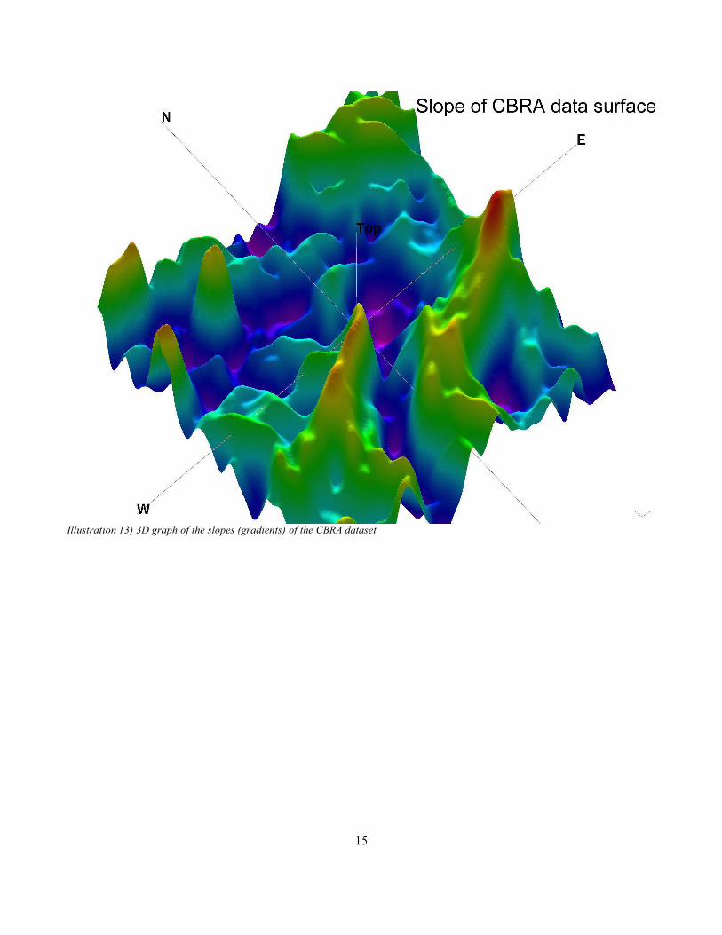
Illustration 13) 3D graph of the slopes (gradients) of the CBRA dataset

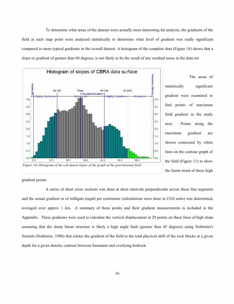
To determine what areas of the dataset were actually most interesting for analysis, the gradients of the

field at each map point were analyzed statistically to determine what level of gradient was really significant

compared to more typical gradients in the overall dataset. A histogram of the complete data (Figure 14) shows that a

slope or gradient of greater than 60 degrees, is not likely to be the result of any residual noise in the data set.

The areas of

statistically significant

gradient were examined to

find points of maximum

field gradient in the study

area. Points along the

maximum gradient are

shown connected by white

lines on the contour graph of

the field (Figure 11) to show

the linear trend of these high

gradient points.

A series of short cross sections was done at short intervals perpendicular across these line segments

and the actual gradient in of milligals (mgal) per centimeter (calculations were done in CGS units) was determined,

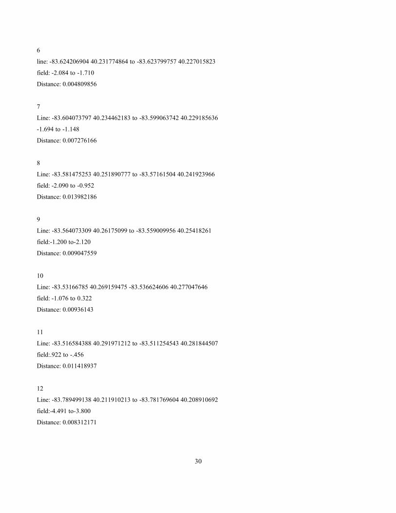
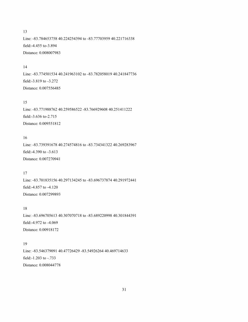
averaged over approx 1 km. A summary of these points and their gradient measurements is included in the

Appendix. These gradients were used to calculate the vertical displacement at 20 points on these lines of high slope

assuming that the sharp linear structure is likely a high angle fault (greater than 45 degrees) using Noltimier's

formula (Noltimier, 1996) that relates the gradient of the field to the total physical shift of the rock blocks at a given

depth for a given density contrast between basement and overlying bedrock.

16

Figure 14) Histogram of the calculated slopes of the graph of the gravitational field

Z 1=Z 0e[[ g / y]/G]Z1 is the depth to the downdropped slab relative to Z0, the higher side of the slab.

Δg is the maximum gradient of the gravitational field in mGal/cm.

Δy is the horizontal distance across the fault where the gradient is computed.

Δρ is the density contrast of the dense basement slab to the less dense rock on top of it.

A complete derivation of this formula is to be found in Noltimier (1996).

Two different sets of calculations were done for two different Δρ.

The depth to the shallowest parts of the basement was determined using Paramo's seismic data (from

just north of the area, in Allen County) to be 5700m. This information and these displacements (depths) were

entered into Rockware© as measured "borehole depths". I then used the solid modeling features of the program to

generate a stratigraphic 3D model of the subsurface with Paramo's seismically determined depths used as the depth

Z0 on the upside of each faulted block and Z1, the computed depths entered on the downdropped side of the block.

17

Table 1) Fault throw calculations from Gravity. Z0/Z1 in Km.

p0 p1 Dist (deg) Dist (cm) grad Z0/Z1 Δρ=.15 Z0/Z1Δρ=.2-3.32 -3.78 0.00544829 60585.0 7.46E-009 1.452 1.323-2.59 -2.88 0.00539479 59990.0 4.78E-009 1.270 1.196-2.12 -2.83 0.00891605 99146.5 7.08E-009 1.425 1.304-2.14 -2.8 0.00794781 88379.7 7.52E-009 1.456 1.326-2.18 -2.55 0.00365874 40685.2 8.97E-009 1.566 1.400-1.71 -2.08 0.00480986 53485.6 6.99E-009 1.418 1.300-1.15 -1.69 0.00727617 80911.0 6.75E-009 1.401 1.288-0.95 -2.09 0.01398219 155481.9 7.32E-009 1.442 1.316

-1.2 -2.12 0.00904756 100608.9 9.14E-009 1.579 1.4090.32 -1.08 0.00936143 104099.1 1.34E-008 1.956 1.6540.92 -0.46 0.01141894 126978.6 1.09E-008 1.720 1.502-3.8 -4.49 0.00831217 92431.3 7.48E-009 1.453 1.323

-3.89 -4.46 0.00800798 89048.8 6.30E-009 1.370 1.266-3.27 -3.82 0.00755649 84028.1 6.51E-009 1.384 1.276-2.72 -3.64 0.00955181 106216.1 8.67E-009 1.542 1.384-3.61 -4.39 0.00727094 80852.9 9.61E-009 1.616 1.434-4.12 -4.86 0.00729989 81174.8 9.08E-009 1.574 1.405-4.07 -4.97 0.00918172 102100.7 8.84E-009 1.556 1.393-0.73 -1.2 0.00804478 89457.9 5.25E-009 1.300 1.218-0.28 -1.26 0.01086377 120805.1 8.14E-009 1.502 1.357

18

Figure 15) View of model of crystalline basement from CBRA dataset looking North. including Paleozoic sedimentary rocks andsurface topography.

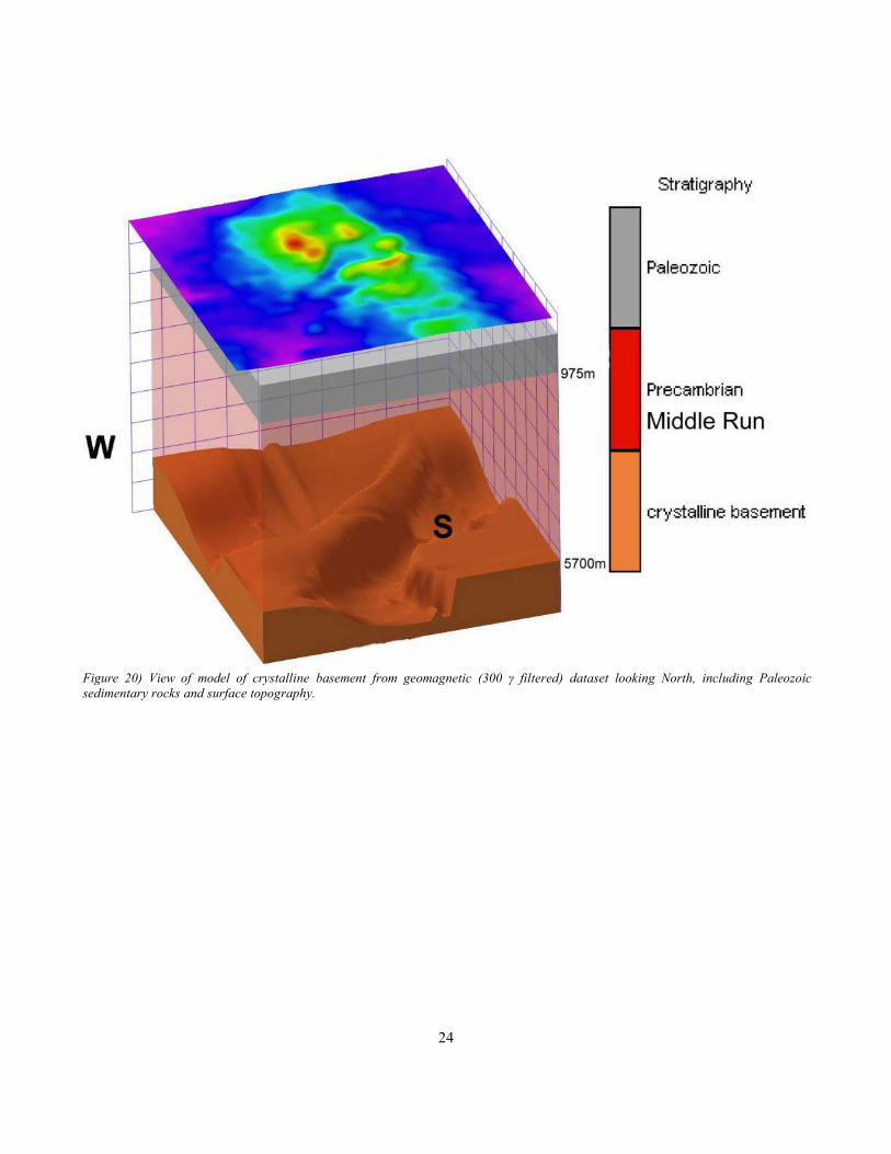
part 5. Basement Model from Geomagnetic data.

To process the Magnetic field data, I used Rockware© software to grid Weaver's 300 gamma (300 γ)

filtered magnetic field data set and produce a contour graph of the data. A second gridded dataset was produced that

has the field magnitude normalized to set the range of the field to be the same as the horizontal size of the graph in

degrees.

19

Figure 16) Contour graph of geomagnetic field (300 γ filtered) dataset with lines of maximum gradient in white. Field contouredin gammas with regional average survey field normalized to 0 gamma.

Then Rockware© was used to determine the field gradient as the slope of the graph in degrees at each

grid point. It is assumed that a high gradient of the field is because of a vertical change in the elevation of the

crystalline basement rocks and not because of a change in the magnetic susceptibility in the Paleozoic sedimentary

rocks.

20

Figure 17) Contour graph of the slope of the 300 γ filtered geomagnetic field dataset.

21

Figure 18) 3D graph of the slopes (gradients) of the geomagnetic 300 γ filtered dataset.

To determine what areas of the dataset were actually most interesting for analysis, the gradients of the

field at each map point were analyzed statistically to determine what level of gradient was really significant

compared to the overall dataset. The magnetic field data were generally less noisy than the gravity data, and the

average rate of magnetic field change in the data set was very small. This made the unusually high points of

gradient stand farther away from the mean of the field gradients than in the gravity data gradients. In this case, any

slope of the graph that was greater than 50 degrees was considered to be anomalous, as it was 3 standard deviations

from the mean slope.

The points of

maximum gradient were

mapped onto the original

magnetic field contour

graph, the same way the

lines were mapped onto the

gravity contour map. These

lines are (again) shown in

white on Figure 16.

A series of short cross sections was done at short intervals perpendicular across these line segments

and the actual gradient in gamma per centimeter was determined averaged over approx 1 km. A summery of these

points and their gradient measurements is included in the Appendix . These gradients were used to calculate the

vertical displacement at 13 points on these lines of high slope, assuming that the sharp linear structure is likely a

high angle fault, using Noltimier's formula (Noltimier, 1997) that relates the gradient of the geomagnetic field to the

22

Figure 19) Histogram of the calculated slopes of the graph of the geomagnetic (300 γ filtered)dataset.

total vertical displacement of the Precambrian basement rock at a given depth for a given magnetic susceptibility

contrast with overlying bedrock.

h=[ z h2J y ]Δh is the change in hight of the downdropped block from the shallowest basement.

h is the depth to the shallowest basement.

Δz is the change of the geomagnetic field across lateral distance Δy. Δz/Δy is the gradient.

J is the magnetic susceptibility of the magnetic crystalline basement rocks. The magnetic susceptibility of the

overlying bedrock is effectively zero by contrast.

A complete derivation of this formula is to be found in Noltimier (1997).

The Depth to the shallowest basement was determined (using Paramo's seismic data from a short

distance north of the survey area, in Allen County) to be 5700 meters. This information and these displacements

(depths) were entered into Rockware© as measured "borehole depths" to use the solid modeling features of the

program to generate a stratigraphic three dimensional model of the subsurface. Paramo's seismically determined

depths were used as the depth on the upside of each faulted block and the computed depths were entered on the

downdropped side of the block.

23

Table 2) Fault throw calculations from geomagnetic 300 γ filtered dataset. Δh in km.

Field at pt 1 Field at pt 2 Δz Δy (km) h² J Δh21 -82 103 0.92224 32.47900 -2.00000 0.95228

-56 -171 115 0.93137 32.47900 -2.00000 1.00130-127 -283 156 1.18540 32.47900 -2.00000 1.03370-152 -297 145 0.96892 32.47900 -2.00000 1.10230-102 -222 120 0.99749 32.47900 -2.00000 0.98834

-95 -224 129 0.96095 32.47900 -2.00000 1.04400-211 -321 110 0.80033 32.47900 -2.00000 1.05640-154 -267 113 0.80399 32.47900 -2.00000 1.06830-208 -262 54 0.72300 32.47900 -2.00000 0.77875-438 -490 52 0.69022 32.47900 -2.00000 0.78212-406 -456 50 0.52775 32.47900 -2.00000 0.87708-402 -466 64 0.63407 32.47900 -2.00000 0.90529-398 -463 65 0.92175 32.47900 -2.00000 0.75669

24

Figure 20) View of model of crystalline basement from geomagnetic (300 γ filtered) dataset looking North, including Paleozoicsedimentary rocks and surface topography.

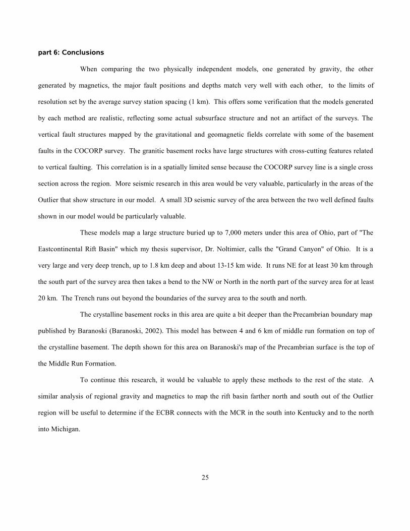
part 6: Conclusions

When comparing the two physically independent models, one generated by gravity, the other

generated by magnetics, the major fault positions and depths match very well with each other, to the limits of

resolution set by the average survey station spacing (1 km). This offers some verification that the models generated

by each method are realistic, reflecting some actual subsurface structure and not an artifact of the surveys. The

vertical fault structures mapped by the gravitational and geomagnetic fields correlate with some of the basement

faults in the COCORP survey. The granitic basement rocks have large structures with cross-cutting features related

to vertical faulting. This correlation is in a spatially limited sense because the COCORP survey line is a single cross

section across the region. More seismic research in this area would be very valuable, particularly in the areas of the

Outlier that show structure in our model. A small 3D seismic survey of the area between the two well defined faults

shown in our model would be particularly valuable.

These models map a large structure buried up to 7,000 meters under this area of Ohio, part of "The

Eastcontinental Rift Basin" which my thesis supervisor, Dr. Noltimier, calls the "Grand Canyon" of Ohio. It is a

very large and very deep trench, up to 1.8 km deep and about 13-15 km wide. It runs NE for at least 30 km through

the south part of the survey area then takes a bend to the NW or North in the north part of the survey area for at least

20 km. The Trench runs out beyond the boundaries of the survey area to the south and north.

The crystalline basement rocks in this area are quite a bit deeper than the Precambrian boundary map

published by Baranoski (Baranoski, 2002). This model has between 4 and 6 km of middle run formation on top of

the crystalline basement. The depth shown for this area on Baranoski's map of the Precambrian surface is the top of

the Middle Run Formation.

To continue this research, it would be valuable to apply these methods to the rest of the state. A

similar analysis of regional gravity and magnetics to map the rift basin farther north and south out of the Outlier

region will be useful to determine if the ECBR connects with the MCR in the south into Kentucky and to the north

into Michigan.

25

References Cited

Baranoski, M.T., 2002. Structure Contour Map on the Precambrian Unconformity Surface inOhio and Related Basement Features, Ohio Department of Natural Resources, Division ofGeological Survey , 20 pp.

Culota, R.C., Pratt, T., and Oliver, J., 1990. A tale of two sutures: COCORP's deep seismicsurveys of the Grenville Province in the eastern U.S. Midcontinent: Geology, v. 18, p646-649.

Hansen, M.C., 1997. GeoFacts no. 13. Ohio Department of Natural Resources, Division ofGeological Survey . 2 pp.

Hansen, M.C., 1998. GeoFacts no. 20. Ohio Department of Natural Resources, Division ofGeological Survey,. 2 pp.

Hansen, M.C., 1989. “How the World Was Made”-The COCORP Traverse of Ohio, OhioGeology Newsletter, Winter 1989, Ohio Department of Natural Resources, Division ofGeological Survey, 8 pp.

Hansen, M.C., 1989. Warren County Deep Core, Ohio Geology Newsletter, Summer 1989,Ohio Department of Natural Resources, Division of Geological Survey, 8 pp.

Kaltenbach, K., 1998. Analysis of Magnetic Anomalies in Determining Fault Displacement inthe Crystalline Precambrian Basement Underneath the Bellefontaine Outlier, Ohio.Senior Thesis, Ohio State University, 61 pp.

Kozlowski, J.D., 1998. Further Correlation of Magnetic Profile Data with Basement Structure ofthe Bellefontaine Outlier, Ohio. Senior Thesis, Ohio State University, 58 pp.

Noltimier, H. C., 1996. Ohio State Univ., Dept. Geol. Sci., GS 683 Gravimetry, course lecturenotes, 29 pp.

Noltimier, H. C., 1997. Ohio State Univ., Dept. Geol. Sci., GS 680 Earth Physics, course lecturenotes, 25 pp.

Paramo, P., 2002. Processing and Interpretation of Seismic Reflection Data: Deep WasteInjection Study, Allen County Ohio. MS Thesis, Ohio State University, 115 pp.

26

Steck, C.D., 1997. Correlation of Gravity Anomalies with Precambrian CrystallineBasement,Bellefontaine Outlier, Ohio, Senior Thesis, Ohio State University, 51 pp.

Weaver, J.P., 1994. A Detailed Gravity and Magnetic Survey of the Bellefontaine Outlier, LoganCounty, Ohio. M.S. Thesis, The Ohio State University, 171 pp.

Wickstrom, L.H., 1990. A new look at Trenton (Ordovician) structure in northwestern Ohio:Northeastern Geology, v. 12, no 3, p. 103-113.

27

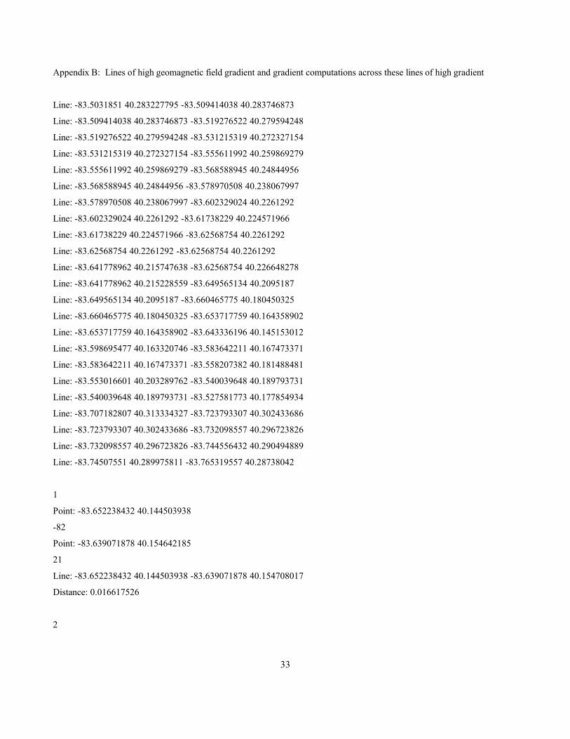
Appendix A

Lines of high gravitational gradient and gradient computations across lines of high gradient.:

Line: -83.504694851 40.286463656 -83.508907943 40.289096839

Line: -83.508907943 40.289096839 -83.512594399 40.286990292

Line: -83.512594399 40.286990292 -83.52154722 40.2827772

Line: -83.52154722 40.2827772 -83.52154722 40.2827772

Line: -83.532079959 40.275404288 -83.521020584 40.2827772

Line: -83.532079951 40.274351015 -83.541559409 40.268031377

Line: -83.541559409 40.268031377 -83.54893232 40.263291648

Line: -83.54893232 40.263291648 -83.558411778 40.258551919

Line: -83.557885141 40.258551919 -83.565784689 40.253285554

Line: -83.565784689 40.253285554 -83.593696426 40.236433185

Line: -83.593696426 40.236433185 -83.605809066 40.227480363

Line: -83.605809066 40.227480363 -83.619501616 40.229060273

Line: -83.619501616 40.229060273 -83.626347891 40.228533637

Line: -83.626347891 40.228533637 -83.634247439 40.225373817

Line: -83.634247439 40.225373817 -83.644253534 40.216947633

Line: -83.644253534 40.216947633 -83.648466626 40.210101358

Line: -83.648466626 40.210101358 -83.656892811 40.196935444

Line: -83.656892811 40.196935444 -83.664265722 40.185876077

Line: -83.677431636 40.172710163 -83.676904999 40.163757342

Line: -83.676904999 40.163757342 -83.666372268 40.14427179

Line: -83.666372268 40.14427179 -83.662159176 40.132685786

Line: -83.691650822 40.305949208 -83.696390551 40.296996387

Line: -83.696390551 40.296996387 -83.70113028 40.292256658

Line: -83.70113028 40.292256658 -83.711663011 40.285937019

Line: -83.711663019 40.285937019 -83.724302288 40.280144017

Line: -83.724302288 40.280144017 -83.734308382 40.274351015

Line: -83.734308382 40.274351015 -83.741154657 40.26750474

Line: -83.741154657 40.26750474 -83.748527569 40.264871558

Line: -83.748527569 40.264871558 -83.752214024 40.264871558

Line: -83.752214024 40.264871558 -83.762220119 40.261185102

Line: -83.762220119 40.261185102 -83.774332759 40.25381219

Line: -83.774332759 40.25381219 -83.773279486 40.248545825

Line: -83.773806122 40.253285554 -83.780125761 40.248545825

28

Line: -83.778545851 40.244332733 -83.778545851 40.22958691

Line: -83.778545851 40.22958691 -83.782232307 40.216420996

Line: -83.782232307 40.216420996 -83.786445398 40.209048085

Line: -83.558309297 40.474817349 -83.543110851 40.472417594

Line: -83.543110851 40.472417594 -83.519913223 40.450019885

Line: -83.556709461 40.449219967 -83.538311342 40.430821848

Gradient computations across these lines of high gradient.

(lines are in decimal degrees, field in Gal, Dist in Km)

1

Line: -83.672032331 40.160158227 to -83.676833343 40.15748488

field: -3.324 to -3.776

Distance: 0.00544829

2

Line: -83.666504992 40.187010133 to -83.661754939 40.184295993

field: -2.876 to-2.589

Distance: 0.005394786

3

line:-83.661890655 40.196788476 to 83.654471525 40.191843534

field: -2.826 to -2.124

Distance: 0.008916049

4

line:-83.65433581 40.209020699 to -83.646780964 40.206418098

field:-2.803 to -2.138

Distance: 0.007947813

5

Line: -83.644202364 40.219393921 to -83.641623764 40.21671696

field: -2.549 to -2.184

Distance: 0.003658738

29

6

line: -83.624206904 40.231774864 to -83.623799757 40.227015823

field: -2.084 to -1.710

Distance: 0.004809856

7

Line: -83.604073797 40.234462183 to -83.599063742 40.229185636

-1.694 to -1.148

Distance: 0.007276166

8

Line: -83.581475253 40.251890777 to -83.57161504 40.241923966

field: -2.090 to -0.952

Distance: 0.013982186

9

Line: -83.564073309 40.26175099 to -83.559009956 40.25418261

field:-1.200 to-2.120

Distance: 0.009047559

10

Line: -83.53166785 40.269159475 -83.536624606 40.277047646

field: -1.076 to 0.322

Distance: 0.00936143

11

Line: -83.516584388 40.291971212 to -83.511254543 40.281844507

field:.922 to -.456

Distance: 0.011418937

12

Line: -83.789499138 40.211910213 to -83.781769604 40.208910692

field:-4.491 to-3.800

Distance: 0.008312171

30

13

Line: -83.784653758 40.224254394 to -83.77703959 40.221716338

field:-4.455 to-3.894

Distance: 0.008007983

14

Line: -83.774501534 40.241963102 to -83.782058019 40.241847736

field:-3.819 to -3.272

Distance: 0.007556485

15

Line: -83.771988762 40.259586522 -83.766929608 40.251411222

field:-3.636 to-2.715

Distance: 0.009551812

16

Line: -83.739391678 40.274574816 to -83.734341322 40.269283967

field:-4.390 to -3.613

Distance: 0.007270941

17

Line: -83.701835156 40.297134245 to -83.696737874 40.291972441

field:-4.857 to -4.120

Distance: 0.007299893

18

Line: -83.696705613 40.307070718 to -83.689220998 40.301844391

field:-4.972 to -4.069

Distance: 0.00918172

19

Line: -83.546379091 40.47726429 -83.54926264 40.469714633

field:-1.203 to -.733

Distance: 0.008044778

31

20

Line: -83.518801873 40.454877461 -83.526456386 40.447065663

field -1.264 to-.281

Distance: 0.01086377

32

Appendix B: Lines of high geomagnetic field gradient and gradient computations across these lines of high gradient

Line: -83.5031851 40.283227795 -83.509414038 40.283746873

Line: -83.509414038 40.283746873 -83.519276522 40.279594248

Line: -83.519276522 40.279594248 -83.531215319 40.272327154

Line: -83.531215319 40.272327154 -83.555611992 40.259869279

Line: -83.555611992 40.259869279 -83.568588945 40.24844956

Line: -83.568588945 40.24844956 -83.578970508 40.238067997

Line: -83.578970508 40.238067997 -83.602329024 40.2261292

Line: -83.602329024 40.2261292 -83.61738229 40.224571966

Line: -83.61738229 40.224571966 -83.62568754 40.2261292

Line: -83.62568754 40.2261292 -83.62568754 40.2261292

Line: -83.641778962 40.215747638 -83.62568754 40.226648278

Line: -83.641778962 40.215228559 -83.649565134 40.2095187

Line: -83.649565134 40.2095187 -83.660465775 40.180450325

Line: -83.660465775 40.180450325 -83.653717759 40.164358902

Line: -83.653717759 40.164358902 -83.643336196 40.145153012

Line: -83.598695477 40.163320746 -83.583642211 40.167473371

Line: -83.583642211 40.167473371 -83.558207382 40.181488481

Line: -83.553016601 40.203289762 -83.540039648 40.189793731

Line: -83.540039648 40.189793731 -83.527581773 40.177854934

Line: -83.707182807 40.313334327 -83.723793307 40.302433686

Line: -83.723793307 40.302433686 -83.732098557 40.296723826

Line: -83.732098557 40.296723826 -83.744556432 40.290494889

Line: -83.74507551 40.289975811 -83.765319557 40.28738042

1

Point: -83.652238432 40.144503938

-82

Point: -83.639071878 40.154642185

21

Line: -83.652238432 40.144503938 -83.639071878 40.154708017

Distance: 0.016617526

2

33

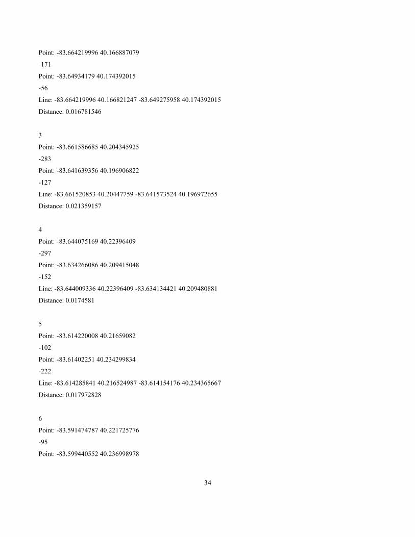
Point: -83.664219996 40.166887079

-171

Point: -83.64934179 40.174392015

-56

Line: -83.664219996 40.166821247 -83.649275958 40.174392015

Distance: 0.016781546

3

Point: -83.661586685 40.204345925

-283

Point: -83.641639356 40.196906822

-127

Line: -83.661520853 40.20447759 -83.641573524 40.196972655

Distance: 0.021359157

4

Point: -83.644075169 40.22396409

-297

Point: -83.634266086 40.209415048

-152

Line: -83.644009336 40.22396409 -83.634134421 40.209480881

Distance: 0.0174581

5

Point: -83.614220008 40.21659082

-102

Point: -83.61402251 40.234299834

-222

Line: -83.614285841 40.216524987 -83.614154176 40.234365667

Distance: 0.017972828

6

Point: -83.591474787 40.221725776

-95

Point: -83.599440552 40.236998978

34

-224

Line: -83.599506385 40.236933145 -83.591408954 40.221659943

Distance: 0.017314519

7

Point: -83.556385921 40.266821222

-321

Point: -83.54921015 40.254444661

-211

Line: -83.556320089 40.266689556 -83.54921015 40.254312996

Distance: 0.014420382

8

Point: -83.526596594 40.266887055

-154

Point: -83.533904031 40.279329448

-267

Line: -83.533838198 40.279329448 -83.526596594 40.266755389

Distance: 0.014486351

9

Point: -83.506748014 40.276893635

-208

Point: -83.504246369 40.289665193

-262

Line: -83.504114703 40.289665193 -83.506682181 40.276827803

Distance: 0.013027072

second fault---

10

Point: -83.764498041 40.294142803

-490

Point: -83.762000326 40.281936229

-438

Line: -83.764498041 40.294102518 -83.76196004 40.281976515

35

Distance: 0.012436484

11

Point: -83.734706748 40.299943948

-456

Point: -83.729389033 40.292128517

-406

Line: -83.734666462 40.299984233 -83.729348747 40.292128517

Distance: 0.009508967

12

Point: -83.716356601 40.301917948

-402

Point: -83.721674316 40.311989379

-466

Line: -83.721674316 40.311989379 -83.716316315 40.301877662

Distance: 0.01142475

13

Point: -83.715289029 40.317548809

-463

Point: -83.703646455 40.305906235

-398

Line: -83.715289029 40.317589095 -83.703606169 40.305825663

Distance: 0.016608129

36