A Semiparametric Negative Binomial Generalized Linear Model for Modeling Over-Dispersed Count Data with a Heavy Tail:

Characteristics and Applications to Crash Data

Mohammadali Shirazi Zachry Department of Civil Engineering

Texas A&M University, College Station, TX 77843, United States Email: alishirazi@tamu.edu

Dominique Lord*, Ph.D. Professor, Zachry Department of Civil Engineering

Texas A&M University, College Station, TX 77843, United States Tel. (979) 458-3949

Email: d-lord@tamu.edu  

Soma Sekhar Dhavala, Ph.D. Chief Data Scientist, Perceptron Learning Solutions Pvt Ltd.

Email: soma.dhavala@gmail.com 

Srinivas Reddy Geedipally, Ph.D. Assistant Research Engineer

Texas A&M Transportation Institute Tel. (817) 462-0519

Email: srinivas-g@tti.tamu.edu

February 21, 2016

*corresponding Author

1  

Abstract

Crash data can often be characterized by over-dispersion, heavy (long) tail and many

observations with the value zero. Over the last few years, a small number of researchers have

started developing and applying novel and innovative multi-parameter models to analyze such

data. These multi-parameter models have been proposed for overcoming the limitations of the

traditional negative binomial (NB) model, which cannot handle this kind of data efficiently. The

research documented in this paper continues the work related to multi-parameter models. The

objective of this paper is to document the development and application of a flexible NB

generalized linear model with randomly distributed mixed effects characterized by the Dirichlet

process (NB-DP) to model crash data. The objective of the study was accomplished using two

datasets. The new model was compared to the NB and the recently introduced model based on

the mixture of the NB and Lindley (NB-L) distributions. Overall, the research study shows that

the NB-DP model offers a better performance than the NB model once data are over-dispersed

and have a heavy tail. The NB-DP performed better than the NB-L when the dataset has a heavy

tail, but a smaller percentage of zeros. However, both models performed similarly when the

dataset contained a large amount of zeros. In addition to a greater flexibility, the NB-DP

provides a clustering by-product that allows the safety analyst to better understand the

characteristics of the data, such as the identification of outliers and sources of dispersion.

Keywords: Negative Binomial, Dirichlet process, Generalized linear model, Crash data 1. Introduction

Regression models have different applications in highway safety. They can be used for

predicting the number of crashes, evaluating roadway safety, screening variables and identifying

hazardous sites. As documented in Lord and Mannering (2010) and more recently in Mannering

and Bhat (2014), extensive research studies have been devoted to develop innovative and novel

statistical models to estimate or predict the number of crashes and evaluate roadway safety.

These statistical models specifically deal with unique characteristics that are associated with

crash data. As such, crash data can often be characterized with over-dispersion, heavy tail and

many observations with the value zero. These unique characteristics inspired a few researchers to

propose several new models that aimed at overcoming the limitations associated with the most

2  

commonly used model in highway safety literature, the negative binomial (NB) model (also

known as the Poisson-gamma model).

Recent research has shown that the NB model can be significantly affected by datasets

characterized by a heavy tail (Zou et al., 2015). According to Guo and Trivedi (2002), the NB

regression model cannot properly capture the heavy tail because a negligible probability is

assigned to large counts. Heavy tails can be caused by the data generating process itself (i.e.,

including observations with very large counts), or they can also be attributed to datasets that have

excess zeros. In the latter case, the heavy tails are created by shifting the overall sample mean

closer to zero, which increases the spread of the observations (Lord and Geedipally, 2016). Over

the last two or three years, a new series of multi-parameter models (i.e., models with several

shape/scale parameters) that mixes the NB distribution with other distributions have been

developed for analyzing such datasets. The NB-Lindley (NB-L) model (Geedipally et al., 2012)

and the NB-generalized exponential (NB-GE) (Vangala et al., 2015) are examples of such types

of models. This paper continues describing research in this line of modeling work.

A recurring theme in many multi-parameter models is to consider a mixing distribution at

the heart of the generative model. For example, one can see the NB as a Poisson-Gamma mixture

or the NB-L as a mixture of the NB and the Lindley distributions (note: the Lindley distribution

itself is a mixture of two Gamma distributions). There are primarily three major ingredients to

eliciting such mixtures, which offer a greater degree of flexibility in model construction:

1. The mixing weights: the mixing weights determine the relative weight of the individual

mixing components.

2. The shape and characteristics of the mixing components or the constituent members of the

mixtures, and

3. The level: in the context of hierarchical/multi-level modeling, at which level the mixture

distribution is elicited.

A transportation safety analyst might have a preference to choose or rather not to choose

a particular mixture. In all cases, the analyst is required to make certain assertions about the

mixture components. One way to retain the modeling flexibility and yet not be overly concerned

about the assertions is to express the uncertainty explicitly by considering a random mixing

3  

distribution. The Dirichlet process (DP), a widely used prior in Bayesian nonparametric

literature, allows such representation (Antoniak, 1974; Escobar and West, 1995). One way to

think about the DP is as an infinite mixture distribution, where the number of unique components

and the component characteristics themselves can be learned from the data.

There has been a phenomenal growth in theory, inference and applications concerning the

DP and its related processes in the last decade; recent monographs on Bayesian nonparametric

devoting significant portion on the DP and related processes is a testimony to that effect (Hjort et

al., 2010; Mitra and Muller, 2015). On the application side, the DP has been applied in numerous

fields ranging from network modeling (Ghosh et al., 2010) to Bioinformatics (Dhavala et al.,

2010; Argiento et al., 2015) to Psychometrics (Miyazaki and Hoshino, 2009) to name a few. In

particular, the application of the DP to account for over-dispersion in count data has been

considered in Mukhopadhyay and Gelfand (1997) and Carota and Parmigiani (2002), with

Binomial and Poisson based likelihoods. More details about the DP, its structure and

computational details are discussed in Sections 2 and 6.

The objective of this study is to develop and document a new method to model over-

dispersed data with a heavy tail. The model is introduced based on the Bayesian hierarchical

modeling framework as a mixture of the NB distribution and a random distribution characterized

by the DP. The proposed model can be motivated, first, by looking at the NB model as a mixture

of the Poisson and Gamma distributions. As an extension of the Poisson model, the Poisson-

gamma was developed assuming that the Poisson parameter is measured with a random error;

this random error itself is gamma distributed. The Poisson-gamma mixture is thought to be a

better alternative to accommodate possible over-dispersion in data (Hilbe, 2011). Second, it can

be motivated by looking at the NB-L model as a mixture of the negative binomial and the

Lindley distributions. The NB-L model can overcome the NB limitations when data are over-

dispersed and have many zeros. Essentially, as discussed above, although mixture models are

providing better alternatives, they assume the shape and density of the distributions to be fixed.

However, we can obtain even more flexibility by assuming that the mixing distribution itself is

random. Given this motivation in mind, the current research plans to develop a model as a

mixture of the negative binomial and a random distribution characterized by the DP.

4  

In addition to providing greater flexibility, the proposed model groups crash data into a

finite number of clusters as one of its by-products. The clustering property of the mixture model

can lend insights to learn more about the domain or the data. This can be used to 1) identify

outliers; 2) study the sites that fall into the same clusters to identify the safety issues and get

insights to implement appropriate countermeasures; and 3) examine sources of dispersions (Peng

et al., 2014).

2. Characteristics of the Dirichlet Process (DP)

Traditionally, the Bayesian parametric inference mechanism considers a parametric distribution

. | , where is a finite vector of parameters, as a prior for the unknown parameter.

However, constraining the model within specific parametric families could limit the scope of the

inference. To overcome this difficulty, in context of the Bayesian nonparametric (or

semiparametric) modeling, a random prior distribution is considered for the parameter as

opposed to choosing a prior distribution from a known parametric family. The prior is placed

over infinite-dimension space of distribution functions. In that sense, it gives more flexibility to

the parameter inference mechanism by providing a wide range of prior distributions.

The DP (Ferguson, 1973; Ferguson, 1974) is a stochastic process that is usually used as a

prior in Bayesian nonparametric (or semiparametric) modeling. Escobar and West (1998) define

the DP as a random probability measure over the space of all probability measures. In that sense,

the DP is considered as a distribution over all possible distributions; that is, each draw from the

DP is itself a distribution. Below, we provide a formal definition and characterization of the DP.

For a gentle introduction and motivation to DP as an extension of the finite dimensional mixtures

to infinite dimensional, the interested readers are referred to Teh (2010) and Gelman et al.

(2014).

Let , , . . , be any finite measurable partitions of the parameter space (Θ). Let us

assume be a positive real number and . | ) be a continuous distribution over Θ. Then,

. ~ , . | if and only if (Escobar and West, 1998):

, , … , ~ | , | , … , | (1)

5  

where is defined as the precision (or concentration) parameter and . | as the base (or

baseline) distribution. Note that based on the Dirichlet distribution properties, for each partition

⊂ Θ, we have:

|

| 1 |

1

Therefore, the base distribution | and the precision parameter play significant roles in the

DP definition. The expectation of the random distribution . is the base distribution . | .

Likewise, the precision parameter controls the variance of the random distribution around its

mean. In other words, measures the variability of the target distribution around the base

distribution. As → ∞, we would have . → . | while, on the other hand, as → 0, the

random distribution . would deviate further away from . | .

Equation (1) defines the DP indirectly through the marginal probabilities assigned to

finite number of partitions. Therefore, it gives no intuition on realizations of

. ~ , . | . To simulate random distributions from the DP, however, Sethuraman

(1994) introduced a straightforward stick-breaking constructive representation of this process as

follows:

| ~ 1, , 1,2,… (2-a)

| ~ . | , 1,2, … (2-b)

1 , 1,2, … (2-c)

. ~ , . | ≡ (2-d)

where indicates a degenerate distribution with all its mass at . This construction,

metaphorically, can be considered as breaking a unit length of stick iteratively (Ishwaran and

James, 2001). First, the stick is broken at a random proportion ; an atom is generated from the

base distribution ( ) and is assigned to the length of the stick that was just broken ( . Then,

recursively, the remaining portions of the stick are broken at new proportions ( , ..); new

atoms are generated from the base distribution ( , , ..) and are assigned to each broken length

of the remained sticks ( , , …).

6  

Given the stick-breaking construction of the DP (Equation 2), the mean and variance of

~ . can be calculated as follows (Yang et al., 2010):

| , (3)

| , (4)

As indicated in Equation (2), theoretically, the stick-breaking construction of the DP

includes infinite components (so called clusters); however, practically, the model can be

approximated with its truncated version (TDP) by considering an upper bound on the number of

components (M) as follows (Ishwaran and James, 2001; Ishwaran and Zarepour, 2002):

| ~ 1, , 1,2, . . , (5-a)

| ~ . | , 1,2, … . , (5-b)

1 , 1,2, … , (5-c)

. ~ , , . | ≡ (5-d)

So far, several research studies have tried to estimate the required number of components

(or clusters) (M) in the truncated version of the DP (Ishwaran and James, 2001; Ohlssen et al.,

2007). As a key point, first, the analyst needs to keep in mind that the number of mass points (M)

in the TDP is correlated to the value of the precision parameter ( ). Theoretically, as the value of

increases, the number of clusters that are shared by data points increases; hence, a larger value

for the parameter M is required. Second, the model needs to be approximated to the level that it

can be assumed that the effect of neglected clusters remains negligible 1 ∑ ). Given

these two rationales into account, Ohlssen et al. (2007) showed that the maximum number of

clusters can be approximated by Equation (6) as a function of and the desired - accuracy as

follows:

1log

log 1

(6)

Once the model is approximated to M clusters, needs to be modified using Equation (7) to

make the model identifiable (i.e.: ∑ 1):

7  

1

(7)

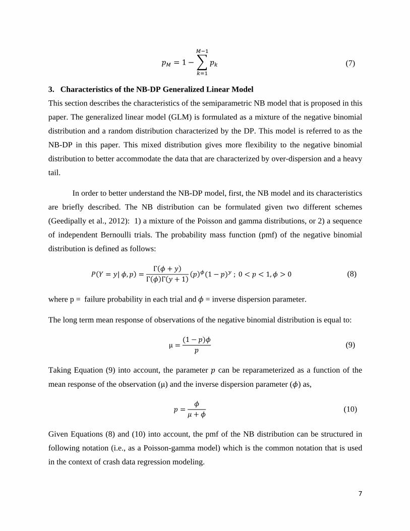
3. Characteristics of the NB-DP Generalized Linear Model

This section describes the characteristics of the semiparametric NB model that is proposed in this

paper. The generalized linear model (GLM) is formulated as a mixture of the negative binomial

distribution and a random distribution characterized by the DP. This model is referred to as the

NB-DP in this paper. This mixed distribution gives more flexibility to the negative binomial

distribution to better accommodate the data that are characterized by over-dispersion and a heavy

tail.

In order to better understand the NB-DP model, first, the NB model and its characteristics

are briefly described. The NB distribution can be formulated given two different schemes

(Geedipally et al., 2012): 1) a mixture of the Poisson and gamma distributions, or 2) a sequence

of independent Bernoulli trials. The probability mass function (pmf) of the negative binomial

distribution is defined as follows:

| ,Γ

Γ Γ 11 ; 0 1, 0 (8)

where p = failure probability in each trial and = inverse dispersion parameter.

The long term mean response of observations of the negative binomial distribution is equal to:

μ1

(9)

Taking Equation (9) into account, the parameter can be reparameterized as a function of the

mean response of the observation (μ) and the inverse dispersion parameter ( ) as,

(10)

Given Equations (8) and (10) into account, the pmf of the NB distribution can be structured in

following notation (i.e., as a Poisson-gamma model) which is the common notation that is used

in the context of crash data regression modeling.

8  

| , ≡ | ,Γ

Γ Γ 11 ; 0 1, 0 (11)

In context of the NB GLM regression for crash data, the long-term mean response of the

NB would have a log-linear relationship with covariates as follows:

ln X (12)

where = j regression coefficient, = d-dimensional observed covariates and = number of

covariates.

The NB-DP distribution can now be defined as a mixture of the NB distribution and a

random distribution characterized by the DP with a precision parameter and a base distribution

. | as follows,

| , , , . | | , | , . | (13)

The structure used to mix the negative binomial distribution and the random distribution

. is similar to the one that was used to introduce the mixture of the negative binomial and

Lindley distribution (Geedipally et al., 2012). In this study, however, instead of the Lindley

distribution, the NB distribution is mixed with a random distribution characterized by the DP to

provide a more flexible model in order to better estimate the long term mean response of the

negative binomial. Nonetheless, since the involved integration in NB-DP model does not have a

closed form, the model cannot (or difficult) to be used with the format shown in Equation (13) to

regress the count data. In order to solve this difficulty, the model was reformulated using the

Bayesian hierarchical scheme as follows:

| , ~ , (14-a)

exp x (14-b)

~ . (14-c)

. ~ , . | (14-d)

9  

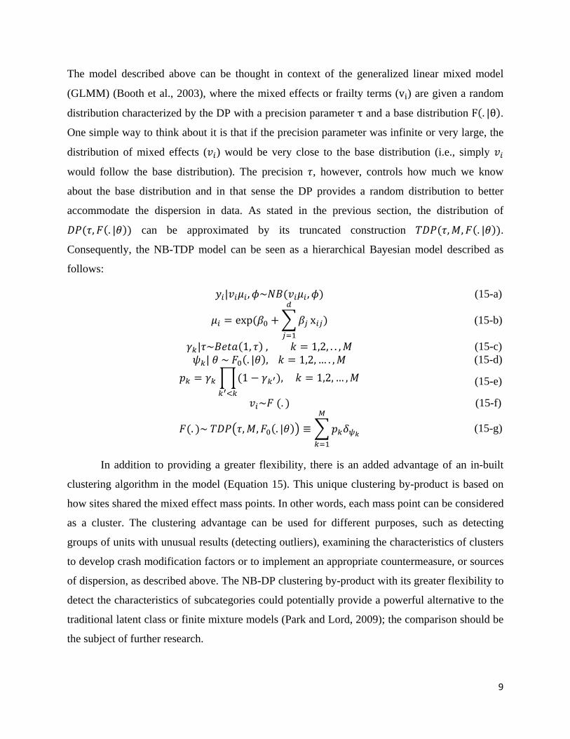
The model described above can be thought in context of the generalized linear mixed model

(GLMM) (Booth et al., 2003), where the mixed effects or frailty terms (v ) are given a random

distribution characterized by the DP with a precision parameter τ and a base distribution F . |θ .

One simple way to think about it is that if the precision parameter was infinite or very large, the

distribution of mixed effects ( ) would be very close to the base distribution (i.e., simply

would follow the base distribution). The precision , however, controls how much we know

about the base distribution and in that sense the DP provides a random distribution to better

accommodate the dispersion in data. As stated in the previous section, the distribution of

, . | can be approximated by its truncated construction , , . | .

Consequently, the NB-TDP model can be seen as a hierarchical Bayesian model described as

follows:

| , ~ , (15-a)

exp x (15-b)

| ~ 1, , 1,2, . . , (15-c) | ~ . | , 1,2, … . , (15-d)

1 , 1,2, … , (15-e)

~ . (15-f)

. ~ , , . | ≡ (15-g)

In addition to providing a greater flexibility, there is an added advantage of an in-built

clustering algorithm in the model (Equation 15). This unique clustering by-product is based on

how sites shared the mixed effect mass points. In other words, each mass point can be considered

as a cluster. The clustering advantage can be used for different purposes, such as detecting

groups of units with unusual results (detecting outliers), examining the characteristics of clusters

to develop crash modification factors or to implement an appropriate countermeasure, or sources

of dispersion, as described above. The NB-DP clustering by-product with its greater flexibility to

detect the characteristics of subcategories could potentially provide a powerful alternative to the

traditional latent class or finite mixture models (Park and Lord, 2009); the comparison should be

the subject of further research.

10  

In order to benefit from the clustering by-product, the hard clustering information (i.e.,

the information about which two data points shared the same mass point or cluster) should be

recorded at each iteration of the Markov Chain Monte Carlo (MCMC) sampling. Let be the

component of the association matrix which is 1 if the data points “m” and “n” belong to the same

cluster and 0 otherwise in the q-th MCMC sample. By definition, Z is symmetric and 1.

Now, the information in matrix Z can be used to elicit the clustering properties and perform

further post-processing analyses (Ohlssen et al, 2007). For instance, the likelihood that site “m”

and site “n” fall into the same cluster can be found by taking an average of over all MCMC

outputs. As another example, the matrix Z can be used to identify outliers. For this purpose, the

variable is defined as ∑ . The variable shows the size of the cluster that

the site “m” belonged to at the q-th iteration of the MCMC. Now, the mean of the cluster size

can be found by taking an average of over all MCMC outputs. Then, by choosing a threshold

(say 3 for example), potential outliers can be detected.

Given an appropriate choice for the DP base distribution, all stages of the model

(Equation 15) would involve only standard distributions. Therefore, the model can be

implemented in a software program, such as WinBUGS (Spiegelhalter et al., 2003) to estimate

the coefficients. Based on how the Bayesian model was parameterized and the definition of the

Dirichlet process, the base distribution is a non-negative distribution that the analyst believes the

frailty terms on average could follow a priori. In this study, we chose a log-normal distribution as

the DP base distribution (i.e., ln ~ , ). Likewise, the analyst must make sure that the

NB-DP model is identifiable (i.e., 1) to eliminate possible correlation between

the intercept ( ) and mixed effects ( ). This issue can be overcome, initially, by dropping the

intercept from the model ( 0 ; then, after the MCMC convergence, the intercept can be

calculated as the log-median of the mixed effects as follows,

ln

In Section 6, we will discuss another intuitive method to overcome the identifiability issue using

the truncated centered Dirichlet process (TCDP) method based on Yang et al.'s (2010) idea to

constrain the mean and variance of the Dirichlet process.

11  

To fully specify the NB-TDP model, we chose a normal prior for and , a gamma

prior for , and a uniform prior for and . Moreover, given Equation (6), if we assume

0.01 and set the upper bound of the uniform prior that is considered for the precision parameter

to 5, the parameter M would approximately be equal to 27. Hence, to round up, we set M=30.

The MCMC was performed with three different chains each with 30,000 iterations. The first

15,000 samples of each chain were regarded as burn-in samples and discarded from the MCMC

outputs. The chains were diagnosed using the Gelman-Rubin (G–R) convergence statistic as well

as the visual observations of the history plots. All chains mixed well and the G–R statistic was

almost 1 for all parameter estimates.

4. Data Description

This section documents the statistics of the datasets that were used in the paper. The datasets

were used to compare the performance of the NB-TDP GLM with NB and NB-L GLMs. The

first subsection briefly describes the summary statistics of the Indiana dataset. The second

subsection summarizes the characteristics of the Michigan dataset. Both datasets are

characterized by high dispersion and have a heavy tail.

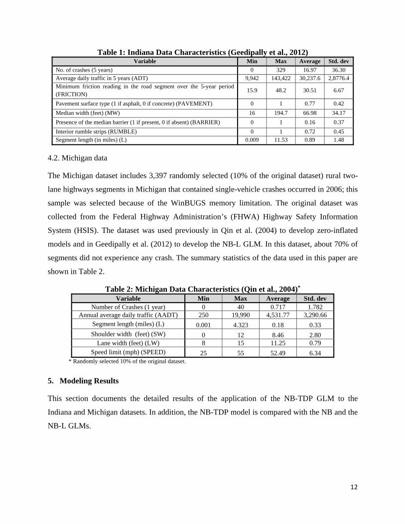
4.1. Indiana data

The Indiana data contain crash, average daily traffic (ADT) and geometric design data collected

for the duration of five-years from 1995 to 1999 at 338 rural interstate road sections in Indiana.

This dataset has been extensively used by others (Anastasopoulos et al., 2008; Washington et al.,

2011; Geedipally et al., 2012). Out of 338 highway segments in this dataset, 120 of them did not

experience any crash (approximately 36% of sites are reported with zero crash). Table 1 shows

the summary statistics of the variables of this dataset. The complete list of variables can be found

in Washington et al. (2011). The Indiana dataset is characterized by a heavy tail that was caused

by the generating process of the data (i.e., the dataset includes observations with very large

values).

12  

Table 1: Indiana Data Characteristics (Geedipally et al., 2012) Variable Min Max Average Std. dev

No. of crashes (5 years) 0 329 16.97 36.30 Average daily traffic in 5 years (ADT) 9,942 143,422 30,237.6 2,8776.4 Minimum friction reading in the road segment over the 5-year period (FRICTION)

15.9 48.2 30.51 6.67

Pavement surface type (1 if asphalt, 0 if concrete) (PAVEMENT) 0 1 0.77 0.42

Median width (feet) (MW) 16 194.7 66.98 34.17

Presence of the median barrier (1 if present, 0 if absent) (BARRIER) 0 1 0.16 0.37

Interior rumble strips (RUMBLE) 0 1 0.72 0.45 Segment length (in miles) (L) 0.009 11.53 0.89 1.48

4.2. Michigan data

The Michigan dataset includes 3,397 randomly selected (10% of the original dataset) rural two-

lane highways segments in Michigan that contained single-vehicle crashes occurred in 2006; this

sample was selected because of the WinBUGS memory limitation. The original dataset was

collected from the Federal Highway Administration’s (FHWA) Highway Safety Information

System (HSIS). The dataset was used previously in Qin et al. (2004) to develop zero-inflated

models and in Geedipally et al. (2012) to develop the NB-L GLM. In this dataset, about 70% of

segments did not experience any crash. The summary statistics of the data used in this paper are

shown in Table 2.

Table 2: Michigan Data Characteristics (Qin et al., 2004)*

Variable Min Max Average Std. dev Number of Crashes (1 year) 0 40 0.717 1.782

Annual average daily traffic (AADT) 250 19,990 4,531.77 3,290.66 Segment length (miles) (L) 0.001 4.323 0.18 0.33 Shoulder width (feet) (SW) 0 12 8.46 2.80

Lane width (feet) (LW) 8 15 11.25 0.79 Speed limit (mph) (SPEED) 25 55 52.49 6.34

* Randomly selected 10% of the original dataset.

5. Modeling Results

This section documents the detailed results of the application of the NB-TDP GLM to the

Indiana and Michigan datasets. In addition, the NB-TDP model is compared with the NB and the

NB-L GLMs.

13  

5.1 Indiana data

In all models, the segment length was considered as an offset; thus, it is assumed that the number

of crashes increases linearly as the segment length increases. Table 3 presents the modeling

results for the Indiana data for the NB, NB-L and NB-TDP GLMs. Given the goodness-of-fit

(GOF) statistics shown in this table, the NB-TDP model showed a better fit compared to other

GLMs. A key point to compare different models together based on GOF measures, however, is

to consider their complexities. The Deviance Information Criterion (DIC) penalizes the model

complexity in its estimate; hence, a more reliable option to employ when models are

characterized by different complexities (as it is in our case). It must be noted that the DIC for

flexible models needs to be calculated with some cautions as it may give rise to bi-modal

marginal distributions for the estimates (Ohlssen et al., 2007). For this reason, WinBUGS does

not calculate the DIC automatically for flexible models. However, similar to what was

experienced in Ohlssen et al. (2007), only a few bimodal distributions were identified for the

estimates; hence, the DIC measure for this model can also be calculated outside of WinBUGS.

The approach discussed in Geedipally et al. (2014) for estimating the DIC was used in this

research. As it is indicated in Table 3, for this dataset, the NB-TDP model showed a better DIC

between the models analyzed.

Table 3: Modeling Results for the Indiana Data

Variable NB NB-L NB-TDP

value Std. dev Value Std. dev value Std. dev

Intercept ( -4.779 0.979 -3.739 1.115 -7.547 1.227 Ln(ADT) ( 0.722 0.091 0.630 0.106 0.983 0.117 Friction ( -0.02774 0.008 -0.02746 0.011 -0.01999 0.008

Pavement ( 0.4613 0.135 0.4327 0.217 0.3942 0.152 MW ( -0.00497 0.001 -0.00616 0.002 -0.00468 0.002

Barrier ( -3.195 0.234 -3.238 0.326 -8.035 1.225 Rumble ( -0.4047 0.131 -0.3976 0.213 -0.3780 0.150

/ 0.934 0.118 0.238 0.083 0.301 0.085 DICa 1900 1701 1638

MADb 6.91 6.89 6.63

MSPEc 206.79 195.54 194.5 a Deviance Information Criterion. b Mean Absolute Deviance (Oh et al., 2003). c Mean Squared Predictive Error (Oh et al., 2003)

14  

For all models, the 95% posterior credible region of none of the parameters includes zero;

hence, all included variables are statistically significant. In addition, all coefficients have the

same and intuitively reasonable sign. However, the estimated coefficient for each model is not

necessary the same. In particular, as a key covariate to predict the number of crashes, different

models estimated different ADT coefficients. The ADT coefficient is below 1 based on the NB

and NB-L modeling results; it is, however, almost 1 based on the NB-TDP modeling results.

Therefore, as the ADT increases, the number of crashes increases at a decreasing rate given the

NB and NB-L estimate while almost linearly given the NB-TDP estimate. The cumulative

residual (CURE) plot can be used to investigate this observation in detail. The cumulative

residual plot estimates how well the proposed model fits data regarding key covariates (Hauer

and Bamfo 1997). A better fit, then, occurs once this plot oscillates more closely around zero.

For a better comparison, the CURE plot is usually adjusted to make the final cumulative value to

be zero. Figure 1 presents the adjusted CURE plot with respect to the ADT covariate (a key

variable to estimate the number of crashes). Figure 1 shows that, with respect to the ADT

covariate, both NB-L and NB-TDP models fit the Indiana data better than the NB model.

Figure 1: CURE Plots for the Indiana Dataset for the ADT Variable (Note: Dotted lines represent ± 2 Std. Dev.)

15  

As discussed in Section 3, as a by-product of the NB-TDP GLM, data can be classified

into finite number of clusters. This clustering property is based on how different sites share the

mixed effect mass points ( ). In order to benefit from the advantage of clustering, the

partitioning information matrix needs to be recorded at each iteration of the MCMC, as discussed

earlier. The matrix can be used to investigate similarities between sites especially with regards to

recognizing unobserved variables (note: in our model, the DP was elicited on mixed effects), or

identifying safety issues and deploying countermeasures.

Let the 338 sites in the Indiana dataset be marked in descending order of ADT values in

numbers from 1 to 338. Figures 2 shows the heatmap representation of the partitioning matrix

for the top 10 sites with the highest ADT values. The figure shows the likelihood that site “X”

and “Y” fall into same cluster. For simplicity, the probabilities were rounded to the first decimal.

A higher likelihood will be represented by a darker shade in the map. As observed in this figure,

for instance, with relatively high probability (~60%), site “1” falls into the same cluster as site

“2”, site “3” or several more. This information can offer insights to identify potential unobserved

variables or safety issues and decide on appropriate countermeasures for the site “1”. On the

other hand, the probability that site “1” falls into the same cluster as site “9” or site “10” is very

small (~10%); hence, there are very few similarities between these sites. In short, the heatmap

can be extended to the entire network and be plotted in a 338×338 dimension matrix, which can

provide a great visual tool to investigate similarities or dissimilarities between sites, at least with

regard to identifying unobserved variables or safety issues. It is worth pointing out that the NB-

TDP GLM, on average, classified the Indiana data into approximately 10 clusters (note: the

posterior estimation of the precision parameter is equal to 2.01).

16  

Figure 2: The Heatmap Representation of the Partitioning Matrix for the Top 10 Sites with the Highest ADT Values in the Indiana Dataset.

5.2 Michigan Data

The functional form that was used in Qin et al. (2004) and Geedipally et al. (2012) to analyze the

original dataset is used here in order to compare the models adequately. Unlike the Indiana data,

the segment length was considered as a covariate in models (i.e., it is not an offset) similar to the

original 2004 paper. However, as shown in Table 4, the coefficient of the segment length is

almost 1 for all models; hence, the number of crashes increases almost linearly once the segment

length increases. Table 4 shows the rest of the modeling results. The sign for all the coefficients

Site  1  2  3  4  5  6  7  8  9  10 

1  1.0  0.6  0.6  0.6  0.6  0.2  0.6  0.6  0.1  0.1 

2  0.6  1.0  0.6  0.6  0.6  0.2  0.6  0.6  0.1  0.1 

3  0.6  0.6  1.0  0.6  0.6  0.2  0.6  0.6  0.1  0.1 

4  0.6  0.6  0.6  1.0  0.6  0.2  0.6  0.6  0.1  0.1 

5  0.6  0.6  0.6  0.6  1.0  0.2  0.6  0.6  0.1  0.1 

6  0.2  0.2  0.2  0.2  0.2  1.0  0.2  0.2  0.6  0.6 

7  0.6  0.6  0.6  0.6  0.6  0.2  1.0  0.6  0.1  0.1 

8  0.6  0.6  0.6  0.6  0.6  0.2  0.6  1.0  0.1  0.1 

9  0.1  0.1  0.1  0.1  0.1  0.6  0.1  0.1  1.0  0.6 

10  0.1  0.1  0.1  0.1  0.1  0.6  0.1  0.1  0.6  1.0 

17  

(those that are statistically significant) are the same as those found in Qin et al. (2004) and were

left as is to be consistent with their work. For this dataset, unlike the Indiana data, different

models estimated relatively similar coefficient values. Table 4 shows that the NB-TDP model

fits data slightly better than the NB and NB-L models based on the Mean Absolute Deviance

(MAD) and Mean Squared Predictive Error (MSPE) GOF measures (Oh et al., 2003). Given the

DIC measure, both NB-L and NB-TDP models (as a class of multi-parameter models) fit the

Michigan data better than the NB model; as discussed above, the DIC is a better measure of fit

for complex hierarchical models than GOF measures based on the model errors since it penalizes

the model complexity. The posterior estimate of the precision parameter for this dataset is

equal to 3.29 and data on average were classified into 21.34 clusters. Note that, intuitively, it is

expected that the crash data be grouped into more clusters once the number of sites in the dataset

increases.

Table 4: Modeling Results for the Michigan Data

Variable NB NB-L NB-TDP

value Std. dev value Std. dev value Std. dev

Intercept ( -3.581 0.6353 -3.508 0.6789 -4.222 0.6711 Ln(ADT) ( 0.4521 0.03935 0.4491 0.04217 0.4739 0.04045

Ln(L) ( 0.942 0.02659 0.940 0.02909 0.968 0.02835 SW( 0.00425a 0.0137 0.00491 0.0144 0.00400 0.0141 LW ( 0.018 0.03664 0.018 0.03916 0.034 0.03878

Speed ( 0.018 0.006298 0.018 0.006629 0.022 0.006836 / 0.6165 0.0617 0.0262 0.0202 0.0303 0.0209

DICb 6223 5796 5984

MADc 0.682 0.689 0.665

MSPEd 1.635 1.641 1.635 a Italic means not statistically significant at the 5% level.

b Deviance Information Criterion. c Mean Absolute Deviance (Oh et al., 2003). d Mean Squared Predictive Error (Oh et al., 2003).

For this dataset, the DIC for the NB-L model is better than the NB-TDP model. This is

due the fact that, first, the NB-L mixture with its fixed distribution is specifically designed to

accommodate data with many zeros (i.e., the NB-L distribution has a large density at zero). The

NB-TDP model, on the other hand, provides more flexibility to capture the variation in data.

Unlike the heavy tail in the Indiana data, which was characterized by a high variation caused by

data points with a large number of crashes as well as a relatively smaller number of zero values

18  

(the range is 329 with ~36% zeros), the heavy tail in the Michigan dataset is characterized by a

large number of zero values (the range is 40 with ~70% zeros). Second, we assumed a uniform

distribution for the precision parameter and set the number of NB-TDP mass points to 30. In this

case, the precision parameter can adapt to the data, and these data can be grouped up to 30

clusters. For cases where the safety analyst would like to attain a better fit, the precision

parameter can be centered around larger values and the NB-TDP can be truncated with a larger

number of mass points (clusters). The latter approach, however, can be problematic to implement

in WinBUGS due to its limitations; hence, the analyst should try other alternatives. Some

alternative approaches to inference the Dirichlet process are discussed in Section 6.

As a closing note, it must be noted that the primary goal in selecting a competitive model

should not be based only on GOF measures. In addition to the GOF, the transportation safety

analyst should examine other issues such as the data generating process, the relationship between

variables and if the proposed model is logically or theoretically sound. The later characteristics

are referred to as “goodness-of-logic” (GOL) in Miaou and Lord (2003).

6. Discussion

The application of the NB-DP or NB-TDP merits important discussion points. Recall that we

have proposed a multi-level hierarchical model to account for over-dispersion and elicited a DP

prior on the random effects to provide modeling flexibility. One of the critical choices we made

was to truncate the Dirichelt process to have finite number of components. Statistical inference

in such complex models is facilitated by employing simulation techniques, such as the MCMC.

We coded the truncated model in WinBUGS to estimate the model’s coefficients (i.e., infer the

parameters). There are several aspects that need to be discussed with building the model and the

subsequent analysis undertaken in this work, namely, truncation and inference, centering and

scaling of the Dirichlet process prior for identifiability and better convergence, and the clustering

property.

There are two major tasks involved in Bayesian model building: model elicitation and

inference. Traditionally, except in very limited cases, Bayesian modeling in general and

Bayesian nonparametric in particular, rely on MCMC for inference, as the models are generally

non-tractable. One of the earliest approaches to inference under the full DP representation was

19  

due to the seminal work by Escobar and West (1995), followed by several others (Escobar and

West, 1998; MacEachern and Muller, 1998). Inference in more complex models, however, was

made possible due to samplers, such as the slice sampling method (Griffin and Walker, 2011;

Kalli et al. 2011). Another interesting avenue was considered by approximating the DP with a

finite sum representation (Ishwaran and Zarepour, 2002). The advantage with the finite sum

based approximation is that, the resulting model is much simpler and often can be fitted using

standard software programs, such as WinBUGS. Consequently, the analyst can focus on trying

several different models without worrying about writing a new sampler or debugging. However,

such approximation comes at a cost: where to truncate? Fortunately, heuristics are available

(Ishwaran and James, 2001; Ohlssen et al., 2007) to provide reasonable results, which may work

very well in practice, as was the case in this study. However, the same benefit of finite sums

representation can be achieved even without truncation, as it is the core idea behind retrospective

sampling (Papaspiliopoulos and Roberts, 2008). In this case, a price that one needs to pay is that

a significant amount of effort is required in designing and developing the samplers, as opposed to

focusing more on model building.

Another very useful approach to approximate inference, the Variational Inference, tries to

approximate the true posterior with its closest parametric counterpart that is much more tractable

analytically (Blei and Jordan, 2006). In fact, off late, approximate inferences as opposed to exact

inferences are becoming popular, such as the Approximate Bayesian Computation (ABC)

framework (Beaumont et al., 2002; Pudlo et al., 2014) and the emerging methods under the

umbrella of Big Data (Neiswanger et al., 2013; Bardenet et al. 2014; Quiroz et al., 2015). The

approximate inference methods can also be found in the frequentist literature (see Bhat, 2014).

The exact approaches to inference can be carried out when the analyst has reasonable

understanding of the domain (or data) with respect to model elicitation. The motivation for

choosing approximate inferential methods is speed and agility, either in model building or fitting

or both. In subsequent work in this area, we will focus on efficient inference mechanisms that

exploit the model characteristics.

An important challenge we faced in this work was the parameterization and

identifiability. As discussed briefly earlier, the intercept term and the mean of the random effects

are correlated. An alternative approach to solve the identifiability issue as well as to obtain a

20  

better convergence properties, is to model the random effects with the TCDP with constrained

variance using the idea proposed in Yang et al. (2010), instead of simple truncated Dirichlet

process. The TCDP model given the precision parameter τ and log-normal base distribution is

structured as:

ln ~ , , ,

If and only if

~ 1, , 1,2, . . , (16-a)

| , ~ , , 1,2, … . , (16-b)

1 , 1,2, … , (16-c)

~ (16-d)

ln (16-e)

where and are defined in Equations (3) and (4) respectively. Therefore,

1

Using the TCDP, not only the median of the mixed effect would be approximately equal to 1, but

we also control the variance of the DP to provide a better convergence. Although the TCDP

model has a nice interpretation and showed very good convergence properties, its

implementation in WinBUGS is very time-consuming for large-scale datasets due to WinBUGS

coding limitations.

Finally, one of defining characteristics of the DP is that it allows for ties in the

observations as the DP is a discrete distribution almost surely. Consequently, during each

iteration of the MCMC, the random affects are partitioned into clusters. This property of the DP

is exploited to post-process MCMC samples to obtain clustering information (Medvedovic and

Sivaganesan, 2002). The clustering information thus obtained can be used to gain further insights

about the problem at hand (for example, which two sites are clustered together). In this regard,

the NB-DP offers great opportunities for analyzing crash data in various different ways. Another

21  

utility of the clustering information is to detect outliers. For example, if one defines an outlier as

belong to a cluster with no more two members in it, then in that regard, singleton clusters can be

defined as outliers and can be inspected for potential risk factors. In fact, the notion of outlier

can be handled much more formally, as is done in Heinzl and Tutz (2013). Indeed, a rich class of

models exist in Bayesian nonparametric, such as the Product Partition Models, when inference

on the partitions is of primary interest (Mitra and Muller, 2015).

7. Summary

This paper has documented the development and application of the NB-DP (or NB-TDP to be

exact) GLM for analyzing over-dispersed crash data characterized by a long or heavy tail. This

new model mixes the NB distribution with a random distribution characterized by the DP. The

model can be thought in context of the Bayesian hierarchical modeling framework, where the

mixed effects are given a flexible distribution. In fact, each draw from the DP is a distribution

and in that sense, instead of being constrained to a particular shape or distribution, a range of

distributions is considered as a prior for random effects. In that regard, it provides more

flexibility for the model to capture the variation in the data as well as handling issues, such as a

heavy tail. The NB-DP was applied to two datasets that were characterized with a heavy tail. The

results were compared with the NB and NB-L models. The results showed that the NB-DP

offered much greatly flexibility and a better fit compared to the NB model. Although the NB-L

might work better with the dataset with many zeros, the NB-DP is actually more flexible to

capture the dispersion in data, especially when the highly dispersed dataset has a heavy tail, but

smaller percentage of zero counts. In addition to a greater flexibility, the proposed model groups

the data points into finite number of clusters. The clustering information can provide further

insights for the transportation safety analyst, such as a better understanding of the data at hand,

identify safety issues and decide on countermeasures.

Acknowledgements

The authors would like to thank Dr. Jeffery Hart from the statistics department of the Texas

A&M University for sharing his valuable insights with us. The paper benefitted from the input of

two anonymous reviewers. Their comments were greatly appreciated.

22  

References

Anastasopoulos, P.C., Tarko, A.P., Mannering, F.L., 2008. Tobit analysis of vehicle accident rates on interstate highways. Accident Analysis & Prevention 40 (2), 768-775.

Antoniak, C.E., 1974. Mixtures of dirichlet processes with applications to bayesian nonparametric problems. Annals of Statistics 2 (6), 1152-1174.

Argiento, R., Guglielmi, A., Hsiao, C., Ruggeri, F., Wang, C., 2015. Modelling the association between clusters of snps and disease responses. . In R. Mitra and P. Mueller (Eds.), Nonparametric Bayesian Methods in Biostatistics and Bioinformatics. Springer.

Bhat, C.R., 2014, The Composite Marginal Likelihood (CML) Inference Approach with Applications to Discrete and Mixed Dependent Variable Models. Foundations and Trends in Econometrics, 7(1), pp. 1-117

Bardenet, R., Doucet, A., Holmes, C., 2014. Towards scaling up markov chain monte carlo: An adaptive subsampling approach. In Proceedings of the 31st International Conference on Machine Learning, 405-413.

Beaumont, M.A., Zhang, W.Y., Balding, D.J., 2002. Approximate bayesian computation in population genetics. Genetics 162 (4), 2025-2035.

Blei, D.M., Jordan, M.I., 2006. Variational inference for dirichlet process mixtures. Bayesian Analysis 1 (1), 121-143.

Booth, J.G., Casella, G., Friedl, H., Hobert, J.P., 2003. Negative binomial loglinear mixed models. Statistical Modelling 3 (3), 179-191.

Carota, C., Parmigiani, G., 2002. Semiparametric regression for count data. Biometrika 89 (2), 265-281.

Dhavala, S.S., Datta, S., Mallick, B.K., Carroll, R.J., Khare, S., Lawhon, S.D., Adams, L.G., 2010. Bayesian modeling of mpss data: Gene expression analysis of bovine salmonella infection. Journal of the American Statistical Association 105 (491), 956-967.

Escobar, M.D., West, M., 1995. Bayesian density-estimation and inference using mixtures. Journal of the American Statistical Association 90 (430), 577-588.

Escobar, M.D., West, M., 1998. Computing nonparametric hierarchical models. Practical Nonparametric and Semiparametric Bayesian Statistics, 1-22.

Ferguson, T.S., 1973. A bayesian analysis of some nonparametric problems. The Annals of Statistics, 209-230.

Ferguson, T.S., 1974. Prior distributions on spaces of probability measures. . The annals of statistics, 615-629.

Geedipally, S.R., Lord, D., Dhavala, S.S., 2012. The negative binomial-lindley generalized linear model: Characteristics and application using crash data. Accident Analysis & Prevention 45, 258-265.

Geedipally, S.R., Lord, D., Dhavala, S.S., 2014. A caution about using deviance information criterion while modeling traffic crashes. Safety Science 62, 495-498.

Gelman, A., Carlin, J., Stern, H., Dunson, D., Vehtari, A., Rubin, D., 2014. Bayesian Data Analysis, CRC Press.

Ghosh, P., Gill, P., Muthukumarana, S., Swartz, T., 2010. A semiparametric bayesian approach to network modelling using dirichlet process prior distributions. Australian & New Zealand Journal of Statistics 52 (3), 289-302.

Griffin, J.E., Walker, S.G., 2011. Posterior simulation of normalized random measure mixtures. Journal of Computational and Graphical Statistics 20 (1), 241-259.

23  

Guo, J.Q., Trivedi, P.K., 2002. Flexible parametric models for long‐tailed patent count distributions*. Oxford bulletin of economics and statistics. 64 1, 63-82.

Hauer, E., Bamfo, J., 1997. Two tools for finding what function links the dependent variable to the explanatory variables. In: Proceedings of the ICTCT 1997 Conference, Lund, Sweden.

Heinzl, F., Tutz, G., 2013. Clustering in linear mixed models with approximate dirichlet process mixtures using em algorithm. Statistical Modelling 13 (1), 41-67.

Hilbe, J.,2011. Negative binomial regression. 2nd Ed. Cambridge : Cambridge University Press, Cambridge.

Hjort, N., Holmes, C., Muller, P., Walker, S., 2010. Bayesian nonparametrics. Cambridge University Press, Cambridge, UK.

Ishwaran, H., James, L.F., 2001. Gibbs sampling methods for stick-breaking priors. Journal of the American Statistical Association 96 (453), 161-173.

Ishwaran, H., Zarepour, M., 2002. Exact and approximate representations for the sum dirichlet process. Canadian Journal of Statistics 30 (2), 269-283.

Kalli, M., Griffin, J.E., Walker, S.G., 2011. Slice sampling mixture models. Statistics and Computing 21 (1), 93-105.

Lord, D., Mannering, F., 2010. The statistical analysis of crash-frequency data: A review and assessment of methodological alternatives. Transportation Research-Part A 44 (5), 291-305.

Lord, D., Geedipally, S.R., 2016. Safety Prediction with Datasets Characterized with Excess Zeros and Long Tails. Forthcoming chapter in book. Emerald Group Publishing Limited, Bingley, UK.

Maceachern, S.N., Muller, P., 1998. Estimating mixture of dirichlet process models. Journal of Computational and Graphical Statistics 7 (2), 223-238.

Mannering, F.L., Bhat, C.R., 2014. Analytic methods in accident research: Methodological frontier and future directions. Analytic Methods in Accident Research 1, 1-22.

Medvedovic, M., Sivaganesan, S., 2002. Bayesian infinite mixture model based clustering of gene expression profiles. Bioinformatics 18 (9), 1194-1206.

Miaou, S.P., Lord, D., 2003. Modeling traffic crash flow relationships for intersections - dispersion parameter, functional form, and bayes versus empirical bayes methods. Transportation Research Record 1840, 31-40.

Mitra, R., Muller, P., 2015. Nonparametric bayesian methods in biostatistics and bioinformatics. Springer-Verlag, New York.

Miyazaki, K., Hoshino, T., 2009. A bayesian semiparametric item response model with dirichlet process priors. Psychometrika 74 (3), 375-393.

Mukhopadhyay, S., Gelfand, A.E., 1997. Dirichlet process mixed generalized linear models. Journal of the American Statistical Association 92 (438), 633-639.

Neiswanger, W., Wang, C., Xing, E., 2013. Asymptotically exact, embarrassingly parallel mcmc. stat 1050 (19).

Oh, J., Lyon, C., Washington, S., Persaud, B., Bared, J., 2003. Validation of fhwa crash models for rural intersections - lessons learned. Transportation Research Record 1840, 41-49.

Ohlssen, D.I., Sharples, L.D., Spiegelhalter, D.J., 2007. Flexible random-effects models using bayesian semi-parametric models: Applications to institutional comparisons. Statistics in Medicine 26 (9), 2088-2112.

24  

Papaspiliopoulos, O., Roberts, G.O., 2008. Retrospective markov chain monte carlo methods for dirichlet process hierarchical models. Biometrika 95 (1), 169-186.

Park, B. J., Lord, D., 2009. Application of finite mixture models for vehicle crash data analysis. Accident Analysis & Prevention, 41(4), 683-691.

Peng, Y., D. Lord, and Y. Zou (2014) Applying the Generalized Waring model for investigating sources of variance in motor vehicle crash analysis. Accident Analysis & Prevention 73, 20-26.

Pudlo, P., Marin, J.M., Estoup, A., Cornuet, J.M., Gautier, M., Robert, C.P., 2014. Abc model choice via random forests. Unpublished paper, Institut de Biologie Computationnelle (IBC), Montpellier, France..

Qin, X., Ivan, J.N., Ravishanker, N., 2004. Selecting exposure measures in crash rate prediction for two-lane highway segments. Accident Analysis and Prevention 36 (2), 183-191.

Quiroz, M., Villani, M., Kohn, R., 2015. Speeding up mcmc by efficient data subsampling. Riksbank Research Paper Series 121.

Sethuraman, J., 1994. A constructive definition of dirichlet priors. Statistica Sinica 4 (2), 639-650.

Spiegelhalter, D.J., Thomas, A., Best, N.G., Lun, D., 2003. Winbugs version 1.4.1 user manual. MRC Biostatistics Unit, Cambridge.

Teh, Y. W., 2010. Dirichlet Processes. Encyclopedia of Machine Learning. Springer Vangala, P., Lord, D., & Geedipally, S. R., 2015. Exploring the application of the Negative

Binomial-Generalized Exponential model for analyzing traffic crash data with excess zeros. Analytic Methods in Accident Research 7, 29-36.

Washington, S., Karlaftis, M., Mannering, F., 2011. Statistical and econometric methods for transportation data analysis,. Chapman and Hall/CRC, Boca Raton, FL.

Yang, M.A., Dunson, D.B., Baird, D., 2010. Semiparametric bayes hierarchical models with mean and variance constraints. Computational Statistics & Data Analysis 54 (9), 2172-2186.

Zou, Y., Wu, L., Lord, D., 2015. Modeling over-dispersed crash data with a long tail: Examining the accuracy of the dispersion parameter in negative binomial models. Analytic Methods in Accident Research 5, 1-16.