A Selection of Physical Chemistry Problems Solved using Mathematica

Housam BINOUS

National Institute of Applied Sciences and Technology

binoushousam@yahoo.com

1- Applied Thermodynamics

2- Chemical Kinetics

Azeotropes for Ternary SystemsCase of Acetone - Chloroform - Methanol System

Gas Constant and

Total Pressure :

Vapor Pressure Using

Antoine Equation :

TC

BAPLog sat

10

R=1.987;P=760;

A1=7.11714;B1=1210.595;C1=229.664;A2=6.95465;B2=1170.966;C2=226.232;A3=8.08097;B3=1582.271;C3=239.726;

PS1=10^(A1-B1/(C1+T));PS2=10^(A2-B2/(C2+T));PS3=10^(A3-B3/(C3+T));

C

ik

jijj

ikiC

jkjjk

x

xx

1

1

1

ln1ln

Liquid phase activity coefficients

from Wilson model :

RTv

v iiij

iL

jLij

exp

l12=116.1171;l21=-506.8519;l13=-114.4047;l31=545.2942;l23=-361.7944;l32=1694.0241;V1=74.05;V2=80.67;V3=40.73;

X3=1.-X1-X2;

A12=V2/V1 Exp[-l12/(R*(273.15+T))];A13=V3/V1 Exp[-l13/(R*(273.15+T))];A32=V2/V3 Exp[-l32/(R*(273.15+T))];A21=V1/V2 Exp[-l21/(R*(273.15+T))];A31=V1/V3 Exp[-l31/(R*(273.15+T))];A23=V3/V2 Exp[-l23/(R*(273.15+T))];

GAM1=Exp[-Log[X1+X2*A12+X3*A13]+1-(X1/(X1+X2*A12+X3*A13)+ X2*A21/(X1*A21+X2+X3*A23)+X3*A31/(X1*A31+X2*A32+X3))];GAM2=Exp[-Log[X1*A21+X2+X3*A23]+1-(X1*A12/(X1+X2*A12+X3*A13)+ X2/(X1*A21+X2+X3*A23)+X3*A32/(X1*A31+X2*A32+X3))];GAM3=Exp[-Log[X1*A31+X2*A32+X3]+1-(X1*A13/(X1+X2*A12+X3*A13)+ X2*A23/(X1*A21+X2+X3*A23)+X3/(X1*A31+X2*A32+X3))];

Modified Raoult’s law :

Using the Mathematica’s function FindRoot to solve a system

of nonlinear equations using different initial guesses :

Y1=X1*PS1*GAM1/P;Y2=X2*PS2*GAM2/P;Y3=X3*PS3*GAM3/P;

In[25]:=FindRoot[{Y1==X1,Y2==X2, P==X1*PS1*GAM1+X2*PS2*GAM2+X3*PS3*GAM3},{X1,0.3},{X2,0.4},{T,40}]

Out[25]={X1->0.329313,X2->0.230369,T->57.3763}In[26]:=FindRoot[{Y1==X1,Y2==X2, P==X1*PS1*GAM1+X2*PS2*GAM2+X3*PS3*GAM3},{X1,0},{X2,0.4},{T,57}]

Out[26]={X1 -> 4.068181432585476 10^-27, X2 -> 0.6547858067091471, T -> 53.89598911261277}In[27]:=FindRoot[{Y1==X1,Y2==X2, P==X1*PS1*GAM1+X2*PS2*GAM2+X3*PS3*GAM3},{X1,0.3},{X2,0},{T,57}]

Out[27]={X1 -> 0.7895499074011907, X2 -> 7.732502667736949 10^-31, T -> 55.37684581029206}In[28]:=FindRoot[{Y1==X1,Y2==X2, P==X1*PS1*GAM1+X2*PS2*GAM2+X3*PS3*GAM3},{X1,0.3},{X2,0.6},{T,63}]

Out[28]={X1->0.337271,X2->0.662729,T->64.5366}

Calculation of Binary Interaction Parameters for Wilson ModelCase of Methanol-Water binary system

P

Pxy

sat

Gas Constant and

Total Pressure :

Modified Raoult’s law with Wilson’s model:

P=760;R=1.987;

A12[T_]:=18.07/40.73 Exp[-d1/(R (T+273.15))];A21[T_]:=40.73/18.07 Exp[-d2/(R (T+273.15))];

y[x_,T_]:=x 10^(Aa-Ba/(T+Ca)) Exp[-Log[x+A12[T] (1-x)] +(1-x) (A12[T]/(x+A12[T] (1-x))-A21[T]/(A21[T] x+1-x))]/P

Aa=8.08097;Ba=1582.271;Ca=239.726;

2

1

expexpexp ),(

N

iiii

cali yTxyMin

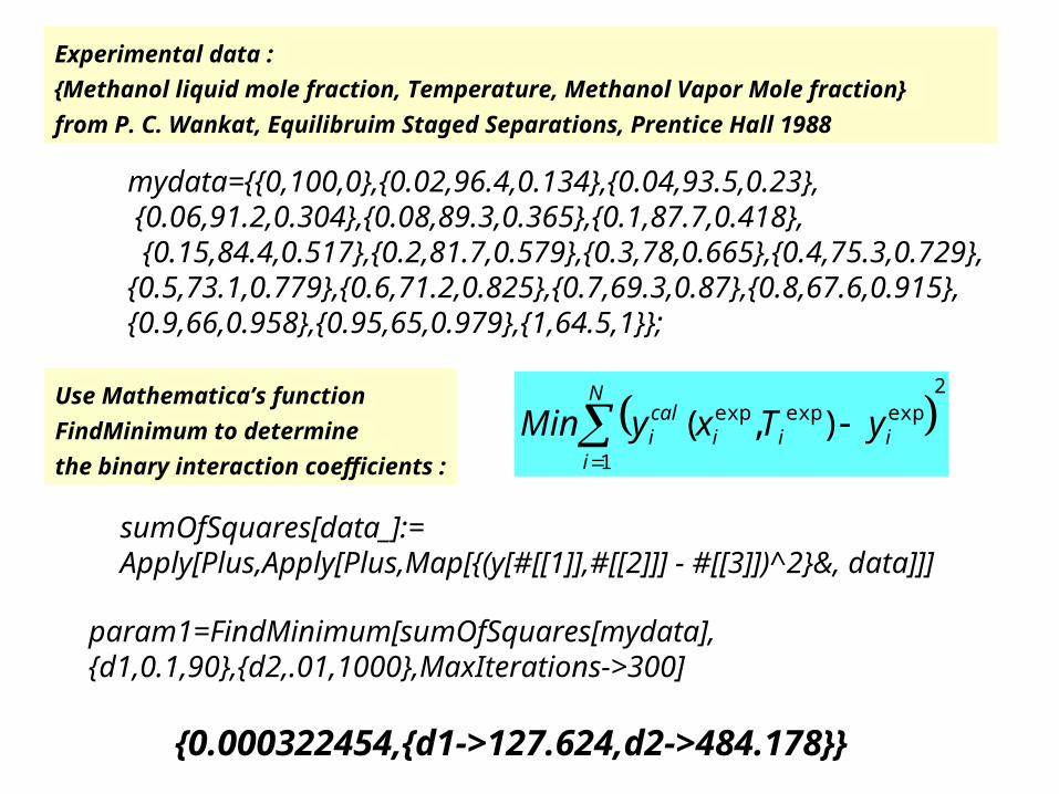
Use Mathematica’s function

FindMinimum to determine

the binary interaction coefficients :

Experimental data :

{Methanol liquid mole fraction, Temperature, Methanol Vapor Mole fraction}

from P. C. Wankat, Equilibruim Staged Separations, Prentice Hall 1988

mydata={{0,100,0},{0.02,96.4,0.134},{0.04,93.5,0.23}, {0.06,91.2,0.304},{0.08,89.3,0.365},{0.1,87.7,0.418}, {0.15,84.4,0.517},{0.2,81.7,0.579},{0.3,78,0.665},{0.4,75.3,0.729},{0.5,73.1,0.779},{0.6,71.2,0.825},{0.7,69.3,0.87},{0.8,67.6,0.915},{0.9,66,0.958},{0.95,65,0.979},{1,64.5,1}};

sumOfSquares[data_]:=Apply[Plus,Apply[Plus,Map[{(y[#[[1]],#[[2]]] - #[[3]])^2}&, data]]]

param1=FindMinimum[sumOfSquares[mydata],{d1,0.1,90},{d2,.01,1000},MaxIterations->300]

{0.000322454,{d1->127.624,d2->484.178}}

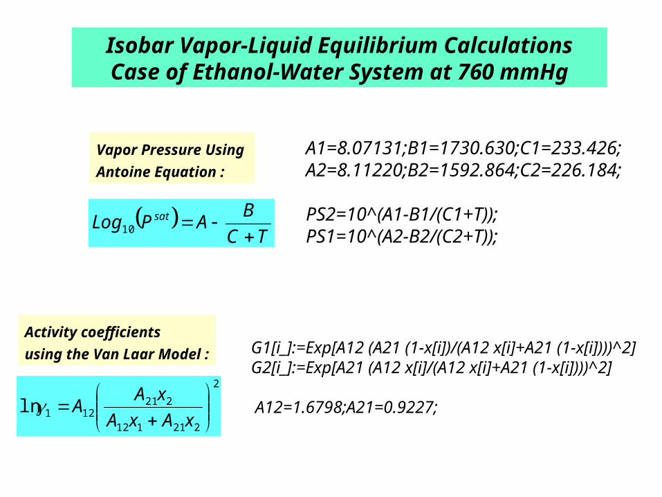
Isobar Vapor-Liquid Equilibrium CalculationsCase of Ethanol-Water System at 760 mmHg

Vapor Pressure Using

Antoine Equation :

TC

BAPLog sat

10

Activity coefficients

using the Van Laar Model :

2

221112

221121ln

xAxA

xAA

A1=8.07131;B1=1730.630;C1=233.426;A2=8.11220;B2=1592.864;C2=226.184;

PS2=10^(A1-B1/(C1+T));PS1=10^(A2-B2/(C2+T));

G1[i_]:=Exp[A12 (A21 (1-x[i])/(A12 x[i]+A21 (1-x[i])))^2]G2[i_]:=Exp[A21 (A12 x[i]/(A12 x[i]+A21 (1-x[i])))^2]

A12=1.6798;A21=0.9227;

Compute T and y for given x using a While loop

and Mathematica’s function FindRoot :

Create tables using Mathematica’s command Table :

i=0;P=760;T=.

While[i<101,{x[i]=i 0.01, T[i]=FindRoot[P== PS1 G1[i] x[i]+PS2 G2[i] (1-x[i]),{T,80}][[1,2]], y[i]=PS1 G1[i] x[i]/P/.T-> T[i],i++}]

tb=Table[{x[i],y[i]},{i,0,100}];tb2=Table[{x[i],T[i]},{i,0,100}];tb3=Table[{y[i],T[i]},{i,0,100}];

Mathematica’s commands ListPlot and Show are used to plot

Bubble point and dew point temperatures on the same figure :

0.2 0.4 0.6 0.8 1

85

90

95

100

x,y

T

plt1=ListPlot[tb2,PlotStyle->RGBColor[1,0,0],PlotJoined-> True, PlotRange->All]

plt2=ListPlot[tb3,PlotStyle->RGBColor[0,0,1],PlotJoined-> True, PlotRange->All]

0.2 0.4 0.6 0.8 1

0.2

0.4

0.6

0.8

1

Mathematica’s commands ListPlot, Line and Epilog are used to plot

the VLE data and the y=x line :

x

y

plt1=ListPlot[tb,PlotStyle->RGBColor[1,0,0],PlotJoined-> True, Epilog-> {RGBColor[0,1,0],Line[{{0,0},{1,1}}]}]

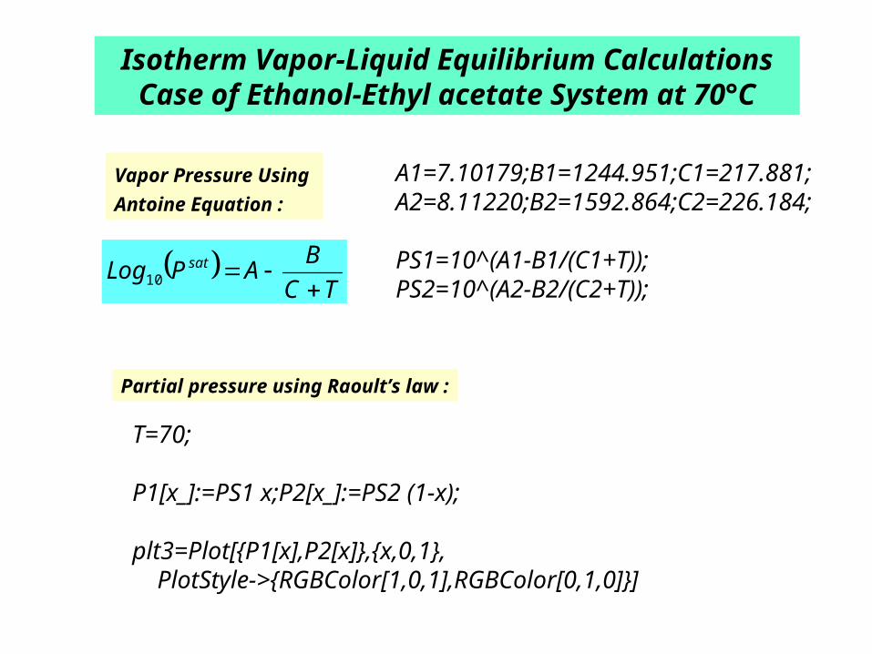
Isotherm Vapor-Liquid Equilibrium CalculationsCase of Ethanol-Ethyl acetate System at 70°C

Vapor Pressure Using

Antoine Equation :

TC

BAPLog sat

10

Partial pressure using Raoult’s law :

A1=7.10179;B1=1244.951;C1=217.881;A2=8.11220;B2=1592.864;C2=226.184;

PS1=10^(A1-B1/(C1+T));PS2=10^(A2-B2/(C2+T));

T=70;

P1[x_]:=PS1 x;P2[x_]:=PS2 (1-x);

plt3=Plot[{P1[x],P2[x]},{x,0,1}, PlotStyle->{RGBColor[1,0,1],RGBColor[0,1,0]}]

Liquid activity coefficients using the Margules Model :

2211221121 )2(ln xxAAA

0.2 0.4 0.6 0.8 1

1.2

1.4

1.6

1.8

2

2.2

Expect positive deviation

from ideality because activity

coefficients are greater than 1 :

x

i

A12=0.8557;A21=0.7476;

G3=Exp[(A12+2 (A21-A12) x) (1-x)^2]G4=Exp[(A21+2 (A12-A21) (1-x)) x^2]

plt8=Plot[{G3,G4},{x,0,1},PlotStyle->{RGBColor[0,0,1],RGBColor[0,0,1]}]

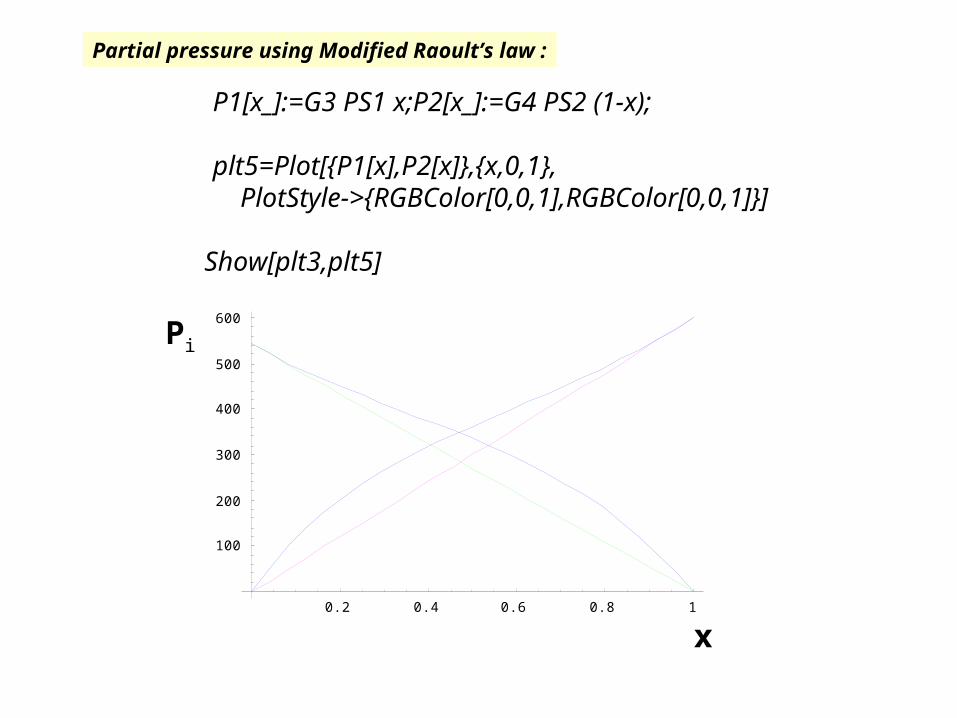
Partial pressure using Modified Raoult’s law :

x

Pi

0.2 0.4 0.6 0.8 1

100

200

300

400

500

600

P1[x_]:=G3 PS1 x;P2[x_]:=G4 PS2 (1-x);

plt5=Plot[{P1[x],P2[x]},{x,0,1}, PlotStyle->{RGBColor[0,0,1],RGBColor[0,0,1]}]

Show[plt3,plt5]

x,y

P

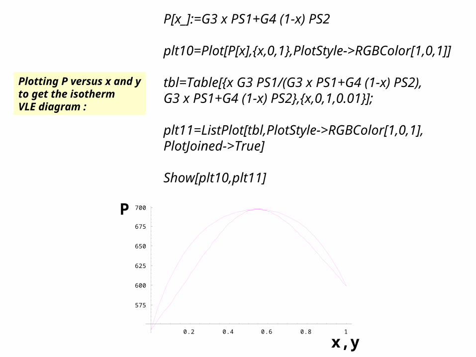
Plotting P versus x and yto get the isotherm VLE diagram :

0.2 0.4 0.6 0.8 1

575

600

625

650

675

700

P[x_]:=G3 x PS1+G4 (1-x) PS2

plt10=Plot[P[x],{x,0,1},PlotStyle->RGBColor[1,0,1]]

tbl=Table[{x G3 PS1/(G3 x PS1+G4 (1-x) PS2),G3 x PS1+G4 (1-x) PS2},{x,0,1,0.01}];

plt11=ListPlot[tbl,PlotStyle->RGBColor[1,0,1],PlotJoined->True]

Show[plt10,plt11]

Wei-Prater mechanism 3-reactant triangle network : A1=A2=A3=A1

with rate constants k12, k21, k23, k32, k31, k13.

Steady state solution obtained using Mathematica’s function Solve :

Rate constants are not independent : k32=k23 (k12/k21) (k31/k13)

k12=.5;k21=0.7;k13=.1;k31=.2;k23=.9;k32=k23 (k12/k21) (k31/k13)A1o=.7;A2o=0;A3o=.3;tf=10;

sequil=Solve[{0==-(k12 +k13) A1+k21 A2+k31 A3 , 0==k12 A1 -(k21 +k23)A2+k32 A3,A3==A1o+A2o+A3o-A1-A2}, {A1,A2,A3}]//Simplify {A1+A2+A3,A2/A1,k12/k21,A3/A1,k13/k31,A3/A2,k23/k32}/.sequil

{{A1->0.451613,A2->0.322581,A3->0.225806}}

{{1.,0.714286,0.714286,0.5,0.5,0.7,0.7}}

transient solution obtained using Mathematica’s function NDSolve :

Plotting the solution using Mathematica’s functions Plot and ParametricPlot :

solWP=NDSolve[{A1'[t]==-(k12 +k13) A1[t]+k21 A2[t]+ k31 (A1o+A2o+A3o-A1[t]-A2[t]) , A2'[t]==k12 A1[t] -(k21 +k23)A2[t]+ k32 (A1o+A2o+A3o-A1[t]-A2[t]), A1[0]==A1o,A2[0]==A2o},{A1[t],A2[t]},{t,0,tf}];

({A1[t],A2[t],A1o+A2o+A3o-A1[t]-A2[t]})/.solWP/.t->tf

{{0.45162,0.322577,0.225802}}

Plot[Evaluate[Table[{A1[t],A2[t],A1o+A2o+A3o-A1[t]-A2[t]}/.solWP]],{t,0,tf}, Frame->True,DefaultFont->{"Symbol-Bold",14}, FrameLabel->{"t","A1, A2, A3"},PlotRange->{{0,tf},{0,1}}, PlotStyle->{RGBColor[1,0,0],RGBColor[0,1,0],RGBColor[0,0,1]}];

ParametricPlot[Evaluate[Table[{A2[t],A1[t]}/.solWP]],{t,0,tf},Frame->True, DefaultFont->{"Symbol-Bold",14},FrameLabel->{"A2","A1"}, PlotRange->{{0,1},{0,1}}];

A

A

A

A

t

A

A

A

Transient solution of Wei-Prater problem :

Consecutive reactions : A1=A2=A3=A4=A5

with rate constants k12, k21, k23, k32, k31, k13...

transient solution obtained using Mathematica’s function NDSolve :

Plotting the transient solution using Mathematica’s functions Plot :

k12=k23=k34=k45=1;k21=k32=k43=k54=.1;A1o=1;tf=10;sol5=NDSolve[{A1'[t]==-k12 A1[t]+k21 A2[t], A2'[t]==k12 A1[t] -(k21 +k23)A2[t]+k32 A3[t], A3'[t]==k23 A2[t] -(k32 +k34)A3[t]+k43 A4[t], A4'[t]==k34 A3[t] -(k43 +k45)A4[t]+k54 (A1o-A1[t]-A2[t]-A3[t]-A4[t]), A1[0]==A1o,A2[0]==0,A3[0]==0,A4[0]==0}, {A1[t],A2[t],A3[t],A4[t]},{t,0,tf}];

Plot[Evaluate[Table[{A1[t],A2[t],A3[t],A4[t],A1o-A1[t]-A2[t]-A3[t]-A4[t]}/.sol5]],{t,0,tf},Frame->True,DefaultFont->{"Symbol-Bold",14},FrameLabel->{"t","A1, A2, A3, A4, A5"},PlotRange->{{0,tf},{0,1}},PlotStyle->{RGBColor[1,0,0],RGBColor[0,1,0],RGBColor[0,0,1], RGBColor[1,1,0],RGBColor[0,1,1]}];

Steady state solution obtained using Mathematica’s function Solve :

Plotting the steady state solution using Mathematica’s functions ListPlot :

soleq=Solve[{0==-k12 A1+k21 A2, 0==k12 A1-(k21 +k23)A2+k32 A3, 0==k23 A2 -(k32 +k34)A3+k43 A4, 0==k34 A3 -(k43 +k45)A4+k54 (A1o-A1-A2-A3-A4)},{A1,A2,A3,A4}]

A5=(A1o-A1-A2-A3-A4)/.soleq

ListPlot[Flatten[{A1,A2,A3,A4,(A1o-A1-A2-A3-A4)}/.soleq], PlotStyle->{PointSize[0.015],RGBColor[1,0,0]}]

t

A

A

A

A

A

transient solution :

Steady state solution :

Lotka-Volterra Mechanism

PY

YYX

XXA

2

2

Foxes and rabbits interactions :

Governing equations :

YkXYkdt

dY

XYkAXkdt

dX

32

21

NDSolve finds the solutions to the ODEs and Plot gives the figure

with typical oscillationsfor the case A=3.7, k1=1.2, k2=1.5 and k3=1.2 :

2 4 6 8 10

1.5

2

2.5

3

t

x,y

A =3.7;k1=1.2;k2=1.5;k3=1.2;

LV=NDSolve[{X'[t]==k1 A X[t]-k2 X[t] Y[t],Y'[t]==k2 X[t] Y[t] -k3 Y[t],X[0]==.85,Y[0]==3.2},{X[t],Y[t]},{t,0,10}];

Plot[Evaluate[Table[{X[t],Y[t]}/.LV]],{t,0,10}, PlotStyle->{RGBColor[1,0,0],RGBColor[0,0,1]}]

fYZ

PX

ZXXA

PYX

XYA

2

2

313

32122

212121

1

1

uuwdt

du

fuuuusdt

du

quuuuusdt

du

Oregonator model of the BZ reaction

Main chemical reactions taking places :

Governing equations :

NDSolve finds the solutions to the ODEs for the case s=100, f=1.1, q=10-6 and w=3.835 :

Plotting the solution using Mathematica’s functions Plot and ParametricPlot :

s=100;f=1.1;q=10^-6;w=3.835;

sol1=NDSolve[{x'[t]==s (x[t]+y[t]-x[t] y[t]-q x[t]^2), y'[t]==1/s (-y[t]-x[t] y[t]+f z[t]), z'[t]==w (x[t]-z[t]), x[0]==1,y[0]==1,z[0]==1},{x,y,z},{t,0,5000}, WorkingPrecision->25,AccuracyGoal->10, PrecisionGoal->10,MaxSteps->Infinity]

pl1=Plot[Evaluate[x[t]/.sol1],{t,0,1000},PlotRange->All, PlotStyle->RGBColor[0,0,1]]

ParametricPlot[Evaluate[{z[t],y[t]}/.sol1],{t,500,1000}, PlotRange->{1,1.20},PlotStyle->RGBColor[0,1,0]]

The solution shows regular oscillations such as those observed in the

Belousov-Zhabotinski experiments. Limit cycle are obtained and a lapse

of time is necessary before oscillations are observed.

10 20 30 40 50

1.02

1.04

1.06

1.08

1.12

1.14

u3

u2

200 400 600 800 1000

10

20

30

40

50

u1

t

Lindermann-Hinshelwood Mechanism

formactivatedinAisA

CBA

AAAA

c

c

c

Quasi steady state approximation :

If A large, reaction rate law is first order

If A small, reaction rate law is second order

Solve[{RA==k1 A^2-k2 A Ac,0==k1 A^2-k2 A Ac-k3 Ac},{RA,Ac}]//Simplify

32

1,

32

31 22

kAk

kAAc

kAk

kkARA

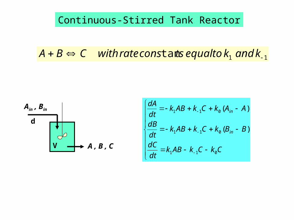
Continuous-Stirred Tank Reactor

11tan kandktoequaltsconsratewithCBA

Ain , Bin

A , B , CV

d

CkCkABkdt

dC

BBkCkABkdt

dB

AAkCkABkdt

dA

in

in

011

011

011

)(

)(

50 100 150 200 250 300

1

2

3

4

5

6

7

8

t

103 C

NDSolve and Plot are used to get the concentration profile of the product :

k1=1;k2=10^-2;k0=d/V;V=10;d=0.6;

sol=NDSolve[{ c'[t]==k1 a[t] b[t]-k2 c[t]-k0 c[t], a'[t]==-k1 a[t] b[t]+k2 c[t]+k0 (0.01-a[t]), b'[t]==-k1 a[t] b[t]+k2 c[t]+k0 (0.02-b[t]), a[0]==10^-2,b[0]==2 10^-2,c[0]==0},{a,b,c},{t,0,300}]

Plot[Evaluate[1000 c[t]/.sol],{t,0,300},PlotRange->{0,8}, PlotStyle->RGBColor[1,0,0]]

Conclusion

Mathematica’s algebraic, numerical and

graphical capabilities can be put into

advantage to solve several Physical Chemistry

problems such as applied thermodynamics

and chemical kinetics.

http://library.wolfram.com/infocenter/search/?search_results=1;search_person_id=1536

http://www.mathworks.com/matlabcentral/fileexchange/loadAuthor.do?objectType=author&objectId=1093893

1/

2/