International Business Research; Vol. 10, No. 11; 2017

ISSN 1913-9004 E-ISSN 1913-9012

Published by Canadian Center of Science and Education

29

A Segmentation Study of Non-Performing Loans Rates in Turkish

Credit Market

Metin Vatansever1, İbrahim Demir

2

1Department of Mathematics, Yildiz Technical University, İstanbul, Turkey

2Department of Statistics, Yildiz Technical University, İstanbul, Turkey

Correspondence: Metin Vatansever, Department of Mathematics, Yildiz Technical University, İstanbul, Turkey.

Received: May 31, 2017 Accepted: September 11, 2017 Online Published: September 29, 2017

doi:10.5539/ibr.v10n11p29 URL: https://doi.org/10.5539/ibr.v10n11p29

Abstract

Non-performing loans (NPLs) rate is one of the main risks in commercial banks and is also a critical measure of

the bank’s financial performance and stability. Banks meet the growth rate of NPLs when the debtors are not able

to meet their financial obligations in terms of repayment of loans. Regional diversification can impact NPLs rate

as well as macroeconomic and bank-specific factors. The purpose of this study is to detect homogeneous credit

risk groups by geographical locations. Diversification across regions can help banks and financial institutions to

determine appropriate market areas and identify effective diversified investment strategies by reducing the overall risk of the credit portfolios.

Keywords: time series clustering, Turkey, credit market, non-performing loans rate

1. Introduction

There is a growing recognition that the quantity or percentage of non-performing loans (NPLs) is related to bank

failures and the financial status of a country. Especially after the global financial crisis of 2007 to 2008, which

started in the US and spread to whole world especially Europe, the issue of non-performing loans (NPLs) has

attracted increasing attention because of the rapidly increased default of sub-prime mortgage loans. Moreover,

there are some evidences that financial and banking crisis in East Asia and Sub-Saharan African countries were

preceded by increasing non-performing loans. In this view of this reality, the non-performing loan ratio is,

therefore, a critical measure to evaluate a bank’s performance, the economic activity, and the national financial stability and soundness.

Lots of factors are responsible for NPLs rate. The literature generally classifies these factors into two parts,

namely: macroeconomic and bank-specific factors. Beside these factors, NPLs rate may vary by region even

under the same economic conditions. From this point of view, the purpose of this study is to find homogeneous

credit risk groups by geographical locations. In particular, a number of hierarchical clustering algorithms (single,

median, average, centroid, complete, ward and weighted) are run to the NPLs rates based on 81 Turkish cities. In

order to choose the right number of cluster and to evaluate clustering results, Silhouette (S), Davies -Bouldin

(DB), Calinski-Harabasz (CH), Dunn (D), Krzanowski-Lai (KL) and Hartigan (Han) validity indices and visual cluster validity (VCV) are used.

The rest of the paper is organized as follows. The second section provides an overview of the literature. Section

three gives the details of the data set and theoretical framework adopted in this paper and section four provides the empirical results. Finally, section five gives a summary of the finding of the study.

2. Literature Review

This section reviews the previous empirical studies on determining factors of the NPLs. There are so many

factors which are responsible for NPLs. The Literature generally divides these factors into two groups. This first

group of literature focuses on the country specific macroeconomic variables such as unemployment, interest rate,

gross domestic product, inflation etc. and the other social variables, which are likely to affect borrowers’

payment capacity to their loans. The second group is called bank-specific factors such as strategy choices,

management excellence, income margins, policy choices, the risk profile of banks etc. (Klein, 2013). Although

there are so many studies to detect factors which are responsible of NPLs, unfortunately there is no any previous study regarding finding homogeneous credit risk groups by geographical locations.

http://ibr.ccsenet.org International Business Research Vol. 10, No. 11; 2017

30

Several studies were done to determine factors of NPLs on different banking systems in different countries. Table 1 indicates NPLs studies which were done in the US

Table 1. Summary of NPLs studies on the US

Paper Variables Period of Data Algorithms Finding

Keeton and Morris (1987)

Loan losses for over 2.400 US commercial banks

1979-1985 Simple linear regression

Local economic conditions, the poor performance of agriculture and energy sectors explain the variation in loan losses in commercial banks of the US.

Sinkey and Greenwalt (1991)

NPLs of big commercial banks in the US

1984-1987 Log-linear regression

Several factors such as high-interest rates, excessive lending and volatile funds as having a positive impact on NPLs of commercial banks in the US.

Gambera (2000) Sample of US banks’ delinquencies

1987-1999 Bivariate VAR models

Farming income, unemployment rate, housing permits, state annual permits and bankruptcy fillings explain the quality of bank asset.

NPLs are not only the problem of America but also the problem of the whole world so we focus on the studies

conducted in the European countries and the rest of the world countries, respectively. Table 2 shows NPLs studies which focus on European countries.

Table 2. Summary of NPLs studies on Europe

Paper Variables Period of

Data

Algorithms Finding

Salas and Saurina(2002)

Loans loss of commercial and saving banks with macroeconomic variables in Spain

1985-1997 Dynamic model Real growth in GDP, rapid credit expansion, bank size, capital ratio and market power explain variation in NPLs

Hoggarth, Sorensen and

Zicchino(2005)

Bank loan loss with macroeconomic variables

in the UK

1988-2004 VAR model Inflation and interest rates have a positive relationship with the

non-performing loans. Chaibi and Ftit i (2015)

NPLs of commercial banks in France and Germany

2005-2011 Dynamic panel data approach

Macro-economic (specifically GDP growth,interest rate, unemployment rate, and exchange rate) and bank-specific variables have an effect on loan quality in the both countries. According to the results, French economy is more susceptible to bank-specific determinants rather than Germany

Kalirai and Scheicher(2002)

NPLs in the Austria banking sector

1990-2001 Linear regression

Short-term nominal interest rate, industrial production, the stock market return and a business confidence index explain loan quality in Austria.

Louzis, Vouldis and Metaxas(2010)

NPLs in 9 largest Greek banks

2003-2009 Dynamic panel data methods

Real GDP growth rate, the unemployment rate and the lending rates are determinants of NPLs

Bofondi and Ropele(2011)

NPLs in Italy

1990-2010 Single-equation time series

NPLs is positively associated with the unemployment rate and the short-term nominal interest rate, while inversely associated with the growth rates of real gross domestic product and house prices.

Berge and Boye(2007)

NPLs in Nordic banking system

1993-2005 ARCH model NPLs are highly associated with the lending and unemployment rates.

Klein (2013) NPLs in different 16 European countries (Central, Eastern and

South-Eastern Europe) with bank-specific and macroeconomic variables

1998-2011 Panel data model

The quality of NPLs can be explained by macroeconomic variables mainly. There is a feedback effect on the loan

quality.

http://ibr.ccsenet.org International Business Research Vol. 10, No. 11; 2017

31

Table 3 points out NPLs studies which concern on developing countries.

Table 3. Summary of NPLs studies on developing countries

Paper Variables Period of

Data

Algorithms Finding

Dash and Kabra(2010)

Macroeconomic and bank specific variables on NPLs of Indian commercial banks

1998-2008 Panel data model

Real income has negative significant effect on NPLs on the other hand high-interest rate incur greater NPLs

Shu (2002) NPLs in Honk Kong 1995-2002 Linear

regression

NPLs is negatively affected by the consumer price inflation rate, gross domestic product

growth, property prices growth, but positively affected by nominal interest rates.

Khemraj and Pasha (2009)

NPLs with macroeconomic and bank-specific variables in

Guyanes banking sector

1994-2004

Panel repression model

The Real effective exchange rate has a positive

relationship with NPLs on the other hand growth in gross domestic product has a negative relationship with NPLs. Moreover,

there is a positive relationship between lending rate and NPLs.

Fofack (2005) NPLs in Sub-Saharan African Countries

Panel-based model

Economic growth, real exchange rate appreciation, the real interest rate, net interest margins, and inter-bank loans have significant effects on NPLs

The above studies are concerned about conventional banking but NPLs are not only the problem of conventional banking system also of Islamic banking. Table 4 indicates NPLs studies on Islamic banking system.

Table 4. Summary of NPLs studies on Islamic banking system

Paper Variables Period of Data Algorithms Finding

Adebola, Wan Yusoff, and

Dahalan (2011)

NPLs in the Islamic banking sector in

Malaysia

2007-2009 ARDL method Interest rate has a positive relationship with NPLs on the other hand producer

price index has a negative relationship with NPLs

Siddiqui, Malik and Shah(2012)

NPLs in Pakistan 1996-2011 Garch Model NPLs are associated with volatility on interest rate

From the above literature review, it is obvious that we can identify the macroeconomic and bank-specific

variables which have a strong relationship with the performance of loans. Otherwise, there is no any prior study

analyzing homogeneous credit risk groups in terms of NPLs rates by geographical locations in Turkey, an

emerging market. At this view, our paper is the initial academic study to analyze groups of cities with similar credit risk on the performance of loans.

3. Turkish Credit Market and Non-Performing Loans

Banking institutions play a very important role in Turkish financial system. According to the last updated 2016

statistics, total banks’ assets are around numbers which is 96 percentage of the total assets of financial systems. Some financial statistics of banking sector are given on Table 5.

Table 5. Financial statistics of banking sector

Billion USD Dolar 1980 1990 1995 2000 2005 2010 2011 2012 2013 2014 2015

Deposit 9 33 45 102 189 400 370 433 443 555 429 Loans 10 27 29 51 114 331 352 433 477 520 500 Assets 19 58 69 155 296 626 614 730 768 812 766 % Loans/GDP - - - 20.5 23.6 46.3 51.2 54.3 64.8 69.2 74.7 % Assets/GDP - - - 62.5 61.2 87.5 89.4 91.6 104.3 108 114.5 % Loans/Assets 53.7 47.0 42.5 32.9 38.6 52.9 57.2 59.2 62.1 64.1 65.2 %Loans/Deposit 109.6 84.0 65.4 50.0 60.4 82.8 95.1 99.9 107.7 114.4 116.6

Source: The Banks Association of Turkey

The financial liberalization process is started in the 1980s in Turkey. During this decade, so many structural

changes occurred in the financial market: abolishing ceilings on interest, setting up interbank money market,

establishing Capital Marked Board (CMB) and Istanbul Stock Exchange (ISE). These liberalization attempts

have enhanced the efficiency, the competition and increased the availability and sources of finance in the financial market, considerably (Yayla, Hekimoğlu and Kutlukaya, 2008).

During the 1990s, although there is a legal regulation in banking and financial services fields, the autonomous

authority are still missing to use this legal regulation. From the point of the necessity, Banking Regulation and

http://ibr.ccsenet.org International Business Research Vol. 10, No. 11; 2017

32

Supervision Agency (BRSA) is founded authority to regulate and supervise the banking sector as the

independent in 2000. All these positive developments make the Turkish banking sector move away from the traditional banking activities (BRSA, 2001).

We can see easily the important financial developments regarding bank balance sheets since the 1980s. Total

assets of the banking sector increased from 19 Billion USD 1980 (62.5 % of GDP) to 766 Billion USD (114.5 %

of GDP) in 2015. Moreover deposit significantly increased from 9 Billion USD in 1980 to 429 Billion USD in

2015, which is 4.667 % increasing. The share of loans in total assets of the banking sector decreased from 47.0 %

in 1990 to about 32.9 % in 2000 and increased to 65.2 % in 2015. The ratio of loans to deposits declined from

84 % in 1990 to 50 % in 2000 and increased to 116.6 % in 2015. The total loans to GDP ratio is increased from

20.5 % in 2000 to about 74.7 % in 2015. Figure 1 shows the development of loans and economic growth of Turkish banking sector.

Figure 1. Development of Loans and Economic Growth (Billion TL)

The Turkish banking sector was severely tested by local and global financial crises in 1994, 2000, 2001 and 2008.

These financial crises badly impact on the Turkish economy and the banking sector. To get a better sense of the banking sector in aggregate loan quality, we look at the loan performance shown in Figure 2.

Figure 2. The Development of NPLs/Total Loans in Turkish Banking Sector

As seen from Figure 2, there are gradual increases in the NPLs rate before the economic crisis 2001 in Turkish

banking sector. NPLs rate is 2.13% in 1997, raised significantly to 37.44% in 2001. Between 1997-2002, 21

banks with poor financial structure were transferred to Saving Deposit Insurance Fund (Yayla, Hekimoğlu and Kutlukaya, 2008).

http://ibr.ccsenet.org International Business Research Vol. 10, No. 11; 2017

33

The main reason for the increase in NPLs rate in Turkish Banking sector is that the regulatory institutions were

not independent from the political authority to regulate and supervise the banking sector effectively. With

establishing Banking Regulation and Supervision Agency (BRSA) NPLs rate falls down significantly (BRSA,

2001). From this point it can be said that Turkish banking sector is completely different before the economic crises in 2001.

4. Data and the Theoretical Framework

In the following subsections, we give a summary of data and such a sort explanation of the theoretical scheme of the time series clustering models and cluster procedures respectively.

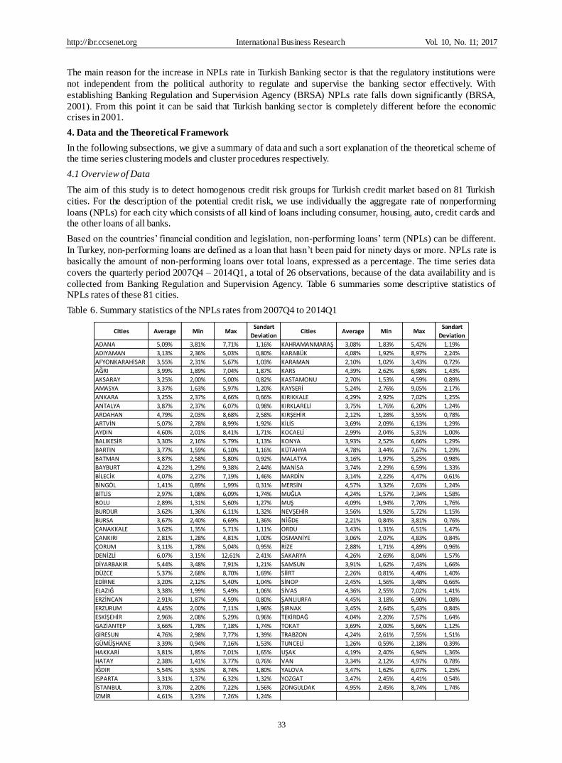
4.1 Overview of Data

The aim of this study is to detect homogenous credit risk groups for Turkish credit market based on 81 Turkish

cities. For the description of the potential credit risk, we use individually the aggregate rate of nonperforming

loans (NPLs) for each city which consists of all kind of loans including consumer, housing, auto, credit cards and the other loans of all banks.

Based on the countries’ financial condition and legislation, non-performing loans’ term (NPLs) can be different.

In Turkey, non-performing loans are defined as a loan that hasn’t been paid for ninety days or more. NPLs rate is

basically the amount of non-performing loans over total loans, expressed as a percentage. The time series data

covers the quarterly period 2007Q4 – 2014Q1, a total of 26 observations, because of the data availability and is

collected from Banking Regulation and Supervision Agency. Table 6 summaries some descriptive statistics of NPLs rates of these 81 cities.

Table 6. Summary statistics of the NPLs rates from 2007Q4 to 2014Q1

Cities Average Min MaxSandart

DeviationCities Average Min Max

Sandart

Deviation

ADANA 5,09% 3,81% 7,71% 1,16% KAHRAMANMARAŞ 3,08% 1,83% 5,42% 1,19%

ADIYAMAN 3,13% 2,36% 5,03% 0,80% KARABÜK 4,08% 1,92% 8,97% 2,24%

AFYONKARAHİSAR 3,55% 2,31% 5,67% 1,03% KARAMAN 2,10% 1,02% 3,43% 0,72%

AĞRI 3,99% 1,89% 7,04% 1,87% KARS 4,39% 2,62% 6,98% 1,43%

AKSARAY 3,25% 2,00% 5,00% 0,82% KASTAMONU 2,70% 1,53% 4,59% 0,89%

AMASYA 3,37% 1,63% 5,97% 1,20% KAYSERİ 5,24% 2,76% 9,05% 2,17%

ANKARA 3,25% 2,37% 4,66% 0,66% KIRIKKALE 4,29% 2,92% 7,02% 1,25%

ANTALYA 3,87% 2,37% 6,07% 0,98% KIRKLARELİ 3,75% 1,76% 6,20% 1,24%

ARDAHAN 4,79% 2,03% 8,68% 2,58% KIRŞEHİR 2,12% 1,28% 3,55% 0,78%

ARTVİN 5,07% 2,78% 8,99% 1,92% KİLİS 3,69% 2,09% 6,13% 1,29%

AYDIN 4,60% 2,01% 8,41% 1,71% KOCAELİ 2,99% 2,04% 5,31% 1,00%

BALIKESİR 3,30% 2,16% 5,79% 1,13% KONYA 3,93% 2,52% 6,66% 1,29%

BARTIN 3,77% 1,59% 6,10% 1,16% KÜTAHYA 4,78% 3,44% 7,67% 1,29%

BATMAN 3,87% 2,58% 5,80% 0,92% MALATYA 3,16% 1,97% 5,25% 0,98%

BAYBURT 4,22% 1,29% 9,38% 2,44% MANİSA 3,74% 2,29% 6,59% 1,33%

BİLECİK 4,07% 2,27% 7,19% 1,46% MARDİN 3,14% 2,22% 4,47% 0,61%

BİNGÖL 1,41% 0,89% 1,99% 0,31% MERSİN 4,57% 3,32% 7,63% 1,24%

BİTLİS 2,97% 1,08% 6,09% 1,74% MUĞLA 4,24% 1,57% 7,34% 1,58%

BOLU 2,89% 1,31% 5,60% 1,27% MUŞ 4,09% 1,94% 7,70% 1,76%

BURDUR 3,62% 1,36% 6,11% 1,32% NEVŞEHİR 3,56% 1,92% 5,72% 1,15%

BURSA 3,67% 2,40% 6,69% 1,36% NİĞDE 2,21% 0,84% 3,81% 0,76%

ÇANAKKALE 3,62% 1,35% 5,71% 1,11% ORDU 3,43% 1,31% 6,51% 1,47%

ÇANKIRI 2,81% 1,28% 4,81% 1,00% OSMANİYE 3,06% 2,07% 4,83% 0,84%

ÇORUM 3,11% 1,78% 5,04% 0,95% RİZE 2,88% 1,71% 4,89% 0,96%

DENİZLİ 6,07% 3,15% 12,61% 2,41% SAKARYA 4,26% 2,69% 8,04% 1,57%

DİYARBAKIR 5,44% 3,48% 7,91% 1,21% SAMSUN 3,91% 1,62% 7,43% 1,66%

DÜZCE 5,37% 2,68% 8,70% 1,69% SİİRT 2,26% 0,81% 4,40% 1,40%

EDİRNE 3,20% 2,12% 5,40% 1,04% SİNOP 2,45% 1,56% 3,48% 0,66%

ELAZIĞ 3,38% 1,99% 5,49% 1,06% SİVAS 4,36% 2,55% 7,02% 1,41%

ERZİNCAN 2,91% 1,87% 4,59% 0,80% ŞANLIURFA 4,45% 3,18% 6,90% 1,08%

ERZURUM 4,45% 2,00% 7,11% 1,96% ŞIRNAK 3,45% 2,64% 5,43% 0,84%

ESKİŞEHİR 2,96% 2,08% 5,29% 0,96% TEKİRDAĞ 4,04% 2,20% 7,57% 1,64%

GAZİANTEP 3,66% 1,78% 7,18% 1,74% TOKAT 3,69% 2,00% 5,66% 1,12%

GİRESUN 4,76% 2,98% 7,77% 1,39% TRABZON 4,24% 2,61% 7,55% 1,51%

GÜMÜŞHANE 3,39% 0,94% 7,16% 1,53% TUNCELİ 1,26% 0,59% 2,18% 0,39%

HAKKARİ 3,81% 1,85% 7,01% 1,65% UŞAK 4,19% 2,40% 6,94% 1,36%

HATAY 2,38% 1,41% 3,77% 0,76% VAN 3,34% 2,12% 4,97% 0,78%

IĞDIR 5,54% 3,53% 8,74% 1,80% YALOVA 3,47% 1,62% 6,07% 1,25%

ISPARTA 3,31% 1,37% 6,32% 1,32% YOZGAT 3,47% 2,45% 4,41% 0,54%

İSTANBUL 3,70% 2,20% 7,22% 1,56% ZONGULDAK 4,95% 2,45% 8,74% 1,74%

İZMİR 4,61% 3,23% 7,26% 1,24%

http://ibr.ccsenet.org International Business Research Vol. 10, No. 11; 2017

34

4.2 Theoretical Framework

4.2.1 Clustering

Time series clustering is an unsupervised technique for finding similar/homogenous groups in data, called

clusters, based on similarity or dissimilarity measures. Hence, time series are similar in the same cluster.

Clustering techniques have been applied to a wide variety of fields such as finance, computer sciences,

engineering, life and medical sciences, earth sciences, social sciences and economics (Xu and Wunsch, 2005).

While many clustering techniques were studied in different domains, most of these techniques are based on the

assumption that data objects can be given as static points in multidimensional spaces. Unfortunately, the

assumption does not always work. As an important class of these problems, time series is a sequence of data

points changed with the time that founded in many application from science, engineering, business, finance, economics, health care to other domains (Liao, 2005).

A wide range of cluster methods is available for the static data in the literature. Han and Kambar (2001) divided

clustering techniques for handling various static data into five main groups: hierarchical, partitioning,

density-based, model-based, and grid-based techniques. Otherwise, diverse algorithms have been evolved to

cluster a bunch of different forms of time series data. As stated by Liao (2005), there are three major approaches

in time series clustering: raw-data-based, feature-based and model-based. The existing static data clustering

algorithms can be applied for the time series data directly. This approach is called raw-data-based clustering. The

main logic of this approach depends on replacing the distance/similarity measure for static data with a suitable

one for time series. Beside this approach, there are feature-based and model-based methods which use features or model parameters of time series for conventional clustering algorithms, respectively (Liao, 2005).

In this study, hierarchical clustering methods are used because of the following reasons: great visualization

feature, the capability of using time series with different length and working without knowing any parameter such as the number of clusters (Xu and Wunsch, 2005 ; Liao, 2005).

Hierarchical clustering technique basically organizes data by creating a tree of clusters based on the distance or

similarity between them. The cluster tree named a dendrogram is generally used to show the process of

hierarchical clustering. It displays how data points are clustered together bit-by-bit. Clustering outcomes can be

kept by cutting the dendrogram at different levels. This representation gives very informative summaries and visualization for the potential data clustering frames (Xu and Wunsch, 2005 ; Liao, 2005).

There are commonly known two groups of hierarchical clustering approaches: agglomerative and divisive. The

agglomerative approach starts by placing each observation in its own clusters and then merges these pair of

initial clusters into larger and larger clusters, until all observations are in a single cluster or until certain final

willed number of clusters fulfilled. The divisive approach does just the inverse of agglomerative hierarchical

clustering by starting with all points in one cluster. It split the cluster into smaller and smaller groups (Han and

Kamber, 2001). Figure 3 displays a dendrogram of divisive hierarchical clustering approach for 7 time series (Keogh and Kasetty, 2003).

Figure 3. A Hierarchical clustering of 7 time series

http://ibr.ccsenet.org International Business Research Vol. 10, No. 11; 2017

35

4.2.2 Clustering Procedure

Raw-data-based time series cluster analysis basically consists of three main steps:

1. Clustering Algorithm Design or Selection: Choosing clustering algorithm affects the quality of

clustering results. Almost all clustering algorithms directly work on proximity (similarity/dissimilarity)

measures, which affect the quality of these results, either. Therefore, it is crucial to carefully select right

proximity measures and cluster algorithms in order to design an appropriate cluster strategy and to get more homogenous clusters (Xu and Wunsch, 2005 ; Liao, 2005).

2. Cluster Validation: Clustering validation is concerned with the evaluation of the goodness of clustering

results. To get good clustering results, it helps to learn which clustering proximity measures and

clustering algorithms should be chosen, how many clusters are hidden in the data, wherever the clusters obtained are meaningful, well separated and homogenous (Xu and Wunsch, 2005 ; Liao, 2005).

3. Result Interpretation: The main purpose of clustering is to provide users meaningful knowledge from the raw data then it can help to solve problems encountered. (Xu and Wunsch, 2005 ;Liao, 2005).

Figure 4. Clustering procedure (Xu and Wunsch, 2009)

Figure 4 presents the three steps of the clustering procedure. Cluster analysis is not a one-shot process. In many cases, it is repetition until finding satisfied cluster results.

5. Development of the Clustering Model and Evaluation of Study Results

As mentioned above, raw-data-based time series cluster procedure consists of three steps. In the first step,

namely clustering algorithm design/selection step, we need to choose right proximity measure (similarity or dissimilarity metric) and clustering algorithm to get more accurate homogeneous results.

In this study, single, median, average, centroid, complete, ward and weighted hierarchical clustering algorithms

are run with proximity measures such as Euclidean, Cityblock, Minkowski, Chebychev, Mahalanobis, Cosine,

correlation and spearman to the 81 Turkish cities’ NPLs rates by using Matlab R2012b statistics toolbox.

Silhouette (S), Davies-Bouldin (DB), Calinski-Harabasz (CH), Dunn (D), Krzanowski-Lai (KL) and Hartigan

(Han) validity indices are run to measures their performance and compared with the result of visual cluster

validity (VCV) All the details of all these algorithms, proximity measures and validity indices can be obtained from the Cluster Validity Analysis Platform (Wang, 2007; Xu and Wunsch II, 2005, 2009).

Silhouette index is used to select right proximity measures with right clustering algorithms as selecting criteria.

Silhouette index ranges from -1 to +1. High values mean that the quality of clustering results is appropriate. On

the other hand, low or negative values means that cluster results are poor. From this point, the highest Silhouette

value indicates that the best clustering algorithm and proximity measures are respectively complete hierarchical clustering algorithm and Euclidean for this data .

The second step in clustering process is cluster validation where we decide optimum the number of clusters and

evaluate whether the goodness of results is satisfying or not. We use Euclidean proximity measure which is the

http://ibr.ccsenet.org International Business Research Vol. 10, No. 11; 2017

36

representative distance measurement to assess the inter-object similarity/dissimilarity in the hierarchical

clustering algorithm, and it is the straight-line distance between data points in multi-dimensional space. It

concentrates on the degree of the distances and data points that are near to each other. In this study, the 81x81

Euclidean distance matrix is chosen as input of clustering, to maximize the distances between heterogeneous

credit markets (similarly minimizing the distance within grouped credit markets). After getting the distance

matrix, we run single, median, average, centroid, complete, ward and weighted hierarchical clustering algorithms

to classify the individual univariate NPLs rates of the 81 Turkish cities into 10 clusters. Then Silhouette (S),

Davies-Bouldin (DB), Calinski-Harabasz (CH), Dunn (D), Krzanowski-Lai (KL) and Hartigan (Han) validity

indices1 are run to determine the number of optimum clusters. Table 7 shows the cluster validity index results

obtained from Matlab Statistics Toolbox and the Cluster Validity Analysis Platform (Wang, 2007).

Table 7. Optimum cluster numbers for 81 NPLs rates

Cluster Algorithms S DB CH D KL Han

Average 2 2 7 2 2 2 Centroid 2 2 7 2 2 2 Complete 2 4 3 2 2 2

Median 2 2 5 2 2 2 Single 2 2 3 2 2 2 Ward 3 2 2 2 2 2 Weighted 2 2 3 2 2 2

In Table 7, Davies-Bouldin and Calinski-Harabasz indices suggest different cluster numbers compared to other

validity indices where Silhouette, Dunn, Krzanowski-Lai and Hartigan indicate two optimum clusters. The

frequency of cluster numbers is 2 that highlight the true number of clusters in these data depended on these

indices. But deciding a convenient cluster number is still exacting problem. In order to overcome this exacting

problem, visual approaches (visual cluster validity) can be applied (Bezdek and Hathaway, 2002). The cluster

validity (VCV) is the one of the visual approaches for multi-dimensional data. The basic logic behind this

approach is to map the data into an image schema, applying the grey or colors scale values to show the important degree of each variable for every data points (Hepşen and Vatansever, 2012).

The VCV approach replaces rows and columns of the similarity/dissimilarity matrix applying the cluster classes

after some clustering algorithms have been run. Otherwise, the original order of data points has been classified

such that the members of every cluster lie in sequential rows and columns of the permuted proximity matrix. It is

obvious that assigned light (dark, depending on the grey scale) squares along the diagonal show compact clusters

indicating well separated from neighboring points. If there is no contain significant clusters in the data then this is easily seen in the image (Hepşen and Vatansever, 2012).

In this paper, the VCV approach is used to evaluate the cluster validity of this data. The input data is directly

calculated from the data as Euclidean distance. The images linked to the results of complete hierarchical clustering algorithm are given in below Figure 5.

Figure 5. Results of complete hierarchical clustering algorithm

1Cluster validation is to measure the goodness of clustering results. There are several numerical measures titled

validity indices that are classified into two categories: external and internal validity indices (Aghabozorgi, Shirkhorshidi and Wah, 2015).

# Cluster: 2

20 40 60 80

20

40

60

80

# Clust: 3

20 40 60 80

20

40

60

80

# Cluster: 4

20 40 60 80

20

40

60

80

# Cluster: 5

20 40 60 80

20

40

60

80

# Cluster: 6

20 40 60 80

20

40

60

80

# Cluster: 7

20 40 60 80

20

40

60

80

# Cluster: 8

20 40 60 80

20

40

60

80

# Cluster: 9

20 40 60 80

20

40

60

80

# Cluster: 10

20 40 60 80

20

40

60

80

http://ibr.ccsenet.org International Business Research Vol. 10, No. 11; 2017

37

It should be understood that, while the data are classified by 2, 3, 4, 5, 6, 7, 8, 9 and 10; this will not inevitably

be indicated in unsupervised clustering, e.g. there may not be enough features to allow the cluster. We can notice

the unclear area in the large dark block with fuzzy boundaries which means the cluster may consist of two or

more overlapped clusters in it with very similar association to each other in Figure 5. Moreover, it is also given

that there are three cluster blocks where diagonal dark blocks are clearer. That gives we have three optimum

clusters on this data set. Figure 7 gives the dendrogram of “Complete” hierarchical cluster algorithm and each color displays each cluster sets for NPLs rates in Turkish credit market.

It is also important to test the how clusters differ from each other. To do this, a one-way ANOVA is done on the data set as shown in table 8.

Table 8. ANOVA test results for clusters

A high value of F-ratio and a low significance value imply that there is a large difference between means of

clusters. As can be seen from table 8, the means for three clusters are quite different (meaning clusters are

statistically different from each other). This result, however, does not provide more information on which group

means are different. From this point, it is a necessity to determine whether all clusters are different each other. In

order to make a multiple comparisons, Tukey, Benferroni, Dunn and Sidák, Fisher and Scheffé tests are used.

According to those test results, all clusters are statistically different from each other. Moreover, figure 6 shows the difference between clusters based on median and quantiles.

Figure 6. Boxplot for three clusters

Figure 7. Dendrogram of complete hierarchical clustering algorithms

http://ibr.ccsenet.org International Business Research Vol. 10, No. 11; 2017

38

The three – cluster partition of the cities reveal a clear NPLs rate separation of credit markets given in Table 10,

11 and 12. Cluster 1 is composed of 8 cities, which have the lowest NPLs rates over the period of 2007Q4 to

2014Q1. 62 cities are grouped in Cluster 2. The rest 11 cities belong to Cluster 3. In those cities, NPLs rates are

separately higher than the other two clusters, so they are described “risky” credit market areas. In this investment

viewpoint for NPLs rates minimization, sub-market divided by NPLs rates has little correlation themselves, so it can be the convenient standard for creditors to make right loans portfolio to diversify potential r isks.

Table 9 shows the basic descriptive statistics for NPLs rates based on clusters. As can be noticed, the lowest

risky cities are all in the cluster 1 (average 2.02%), while the third cluster has the highest risky cities (average

5.14%). Other side, high NPLs rates are related to higher level of risk (standard deviation). The highest level of

risk is in cluster 3 (standard deviation 0.48%) and the lowest level of risk is in cluster 1 (standard deviation 0.32%).

Table 9. Descriptive statistics of all clusters from 2007Q4 to 2014Q1

Clusters Average Standard Deviation

Cluster 1 2,02% 0,32%

Cluster 2 3,65% 0,34% Cluster 3 5,14% 0,48%

Table 10. Descriptive statistics of cluster 2 based on cities from 2007Q4 to 2014Q1

Cluster 2 Cities Average Standart Deviation Cities Average Standard Deviation ADIYAMAN 3,13% 0,80% KARABÜK 4,08% 2,24% AFYONKARAHİSAR 3,55% 1,03% KARS 4,39% 1,43% AĞRI 3,99% 1,87% KASTAMONU 2,70% 0,89% AKSARAY 3,25% 0,82% KIRIKKALE 4,29% 1,25% AMASYA 3,37% 1,20% KIRKLARELİ 3,75% 1,24% ANKARA 3,25% 0,66% KİLİS 3,69% 1,29% ANTALYA 3,87% 0,98% KOCAELİ 2,99% 1,00% AYDIN 4,60% 1,71% KONYA 3,93% 1,29% BALIKESİR 3,30% 1,13% KÜTAHYA 4,78% 1,29% BARTIN 3,77% 1,16% MALATYA 3,16% 0,98% BATMAN 3,87% 0,92% MANİSA 3,74% 1,33% BİLECİK 4,07% 1,46% MARDİN 3,14% 0,61% BİTLİS 2,97% 1,74% MERSİN 4,57% 1,24% BOLU 2,89% 1,27% MUĞLA 4,24% 1,58% BURDUR 3,62% 1,32% MUŞ 4,09% 1,76% BURSA 3,67% 1,36% NEVŞEHİR 3,56% 1,15% ÇANAKKALE 3,62% 1,11% ORDU 3,43% 1,47% ÇANKIRI 2,81% 1,00% OSMANİYE 3,06% 0,84% ÇORUM 3,11% 0,95% RİZE 2,88% 0,96% EDİRNE 3,20% 1,04% SAKARYA 4,26% 1,57% ELAZIĞ 3,38% 1,06% SAMSUN 3,91% 1,66% ERZİNCAN 2,91% 0,80% SİVAS 4,36% 1,41% ERZURUM 4,45% 1,96% ŞANLIURFA 4,45% 1,08% ESKİŞEHİR 2,96% 0,96% ŞIRNAK 3,45% 0,84% GAZİANTEP 3,66% 1,74% TEKİRDAĞ 4,04% 1,64% GÜMÜŞHANE 3,39% 1,53% TOKAT 3,69% 1,12% HAKKARİ 3,81% 1,65% TRABZON 4,24% 1,51% ISPARTA 3,31% 1,32% UŞAK 4,19% 1,36% İSTANBUL 3,70% 1,56% VAN 3,34% 0,78% İZMİR 4,61% 1,24% YALOVA 3,47% 1,25% KAHRAMANMARAŞ 3,08% 1,19% YOZGAT 3,47% 0,54%

Table 11. Descriptive statistics of cluster 1 based on cities from 2007Q4 to 2014Q1

Cluster 1

Cities Average Standard Deviation

BİNGÖL 1,41% 0,31% HATAY 2,38% 0,76% KARAMAN 2,10% 0,72%

KIRŞEHİR 2,12% 0,78% NİĞDE 2,21% 0,76% SİİRT 2,26% 1,40% SİNOP 2,45% 0,66% TUNCELİ 1,26% 0,39%

http://ibr.ccsenet.org International Business Research Vol. 10, No. 11; 2017

39

Table 12. Descriptive statistics of cluster 3 based on cities from 2007Q4 to 2014Q1

Cluster 3

Cities Average Standard Deviation

ADANA 5,09% 1,16% ARDAHAN 4,79% 2,58% ARTVİN 5,07% 1,92% BAYBURT 4,22% 2,44% DENİZLİ 6,07% 2,41% DİYARBAKIR 5,44% 1,21% DÜZCE 5,37% 1,69% GİRESUN 4,76% 1,39% IĞDIR 5,54% 1,80% KAYSERİ 5,24% 2,17% ZONGULDAK 4,95% 1,74%

Different employment conditions can affect the NPLs ratio. Gamberea (2000); Chaibi and Ftiti (2015); Louzis,

Vouldis and Metaxas (2010); Bofondi and Ropele (2011); Berge and Boye (2007) indicate that there is a positive

relationship between NPLs rates and unemployment rates in the USA, France, Germany, Greece, Italy and

Nordic countries, respectively. From this point, to get better understanding about the cities’ NPLs dynamics, we

look at 2013 unemployment rate at the on Table 13. As seen from the table, there is a negative correlation

between NPLs rates and average employment rate in clusters. In conclusion, the credit risk is different under the different employment conditions.

Table 13. Average employment rate for clusters

Clusters Average Employment Rate %

1 48,46 2 46,11 3 43,95

Country Average 45,90

Source: Turkish Statistics Institute

6. Conclusion

The existing literature is generally in interested in finding the effects of macroeconomic and bank-specific

factors on NPLs rates. Besides those factors, NPLs rates may vary by region even under the same economic

conditions. From this point, the aim of this study is to develop homogeneous credit risk groups for 81 cities in Turkey by running numerous hierarchical clustering algorithms.

This research adds to the literature in two aspects. First, it gives new information about Turkey’s credit market in

the context of risk diversification based on the different cities. Second, the time series clustering algorithms are

discussed in this research gives a valuable guideline for bankers and financial intuitions for selecting proper market areas, to manage the potential geographical risk and define efficiently diversified credit politics.

Firstly, the empirical results of this research say the three different group partitions of the cities that declare a

clear NPLs rates distinction of the credit market in Turkey. 8 cities are grouped in Cluster 1, which have the

lowest NPLs rates (average 2.02% NPLs rate). Cluster 2 consists of 62 cities, which is the most crowded group.

The rest 11 cities belong to Cluster 3. In those cities, NPLs rates are relatively higher than the other two groups

(average 5.14% NPLs rate), so they are called risky credit market areas. On the other hand, high NPLs rates

associated with higher levels of risk (standard deviation) and vice versa. Secondly, the results of this study could

not be only practical for understanding the historical NPLs behaviors of cities, but also for banks and financial intuitions to make rational credit politics based on different geographic location conditions.

Acknowledge

This research has been supported by Yıldız Technical University Scientific Research Projects Coordination Department. Project Number: 2015-01-05-DOP02

References

Adebola S. S., Wan Yusoff, S. B., & Dahalan, D. J. (2011). An ARDL Approach to the Determination of

Non-Performing Loans. Kuwait Chapter of Arabian Journal of Business and Management Review, 1(2), 20-30.

Aghabozorgi, S., Shirkhorshidi, A. S., & Wah, T. Y., (2015). Time Series Clustering - A Decade Review. Information Systems, 53, 16-38. https://doi.org/10.1016/j.is.2015.04.007

Banking Regulation and Supervision Agency. (2001). Towards A Sound Turkish Banking Sector. Retrieved from

http://ibr.ccsenet.org International Business Research Vol. 10, No. 11; 2017

40

www.bddk.org.tr

Banking Regulation and Supervision Agency. (2016, Aug). Data Retrieved from http://ebulten.bddk.org.tr/finturk

Berge, T. O., & Boye, K. G. (2007). An Analysis of Bank’s Problem Loans. Norges Bank Economic Bulletin, 78, 65–76.

Bezdek, J. C., & Hathaway, R. J. (2002). VAT A Tool for Visual Assessment of (Cluster) Tendency. Proceedings

of the 2002 International Joint Conference o, Honolulu, 3, 2225-2230. https://doi.org/10.1109/ijcnn.2002.1007487

Bofondi, M., & Ropele, T. (2011). Macroeconomic Determinants of Bad Loans: Evidence from Italian Banks. Occasional Papers, 89. https://doi.org/10.2139/ssrn.1849872

Chaibi, H., & Ftiti, Z. (2015). Credit Risk Determinants: Evidence from a Cross-Country Study. Research in International Business and Finance, 19(3), 165-171. https://doi.org/10.1016/j.ribaf.2014.06.001

Dash, M., & Kabra, G. (2010). The Determinants of Non-Performing Assets in Indian Commercial Bank: An Econometric Study. Middle Eastern Finance and Economics, 7, 94-106.

Fofack, H. L. (2005). Non-performing loans in Sub-Saharan Africa: Causal Analysis and Macroeconomic Implications. World Bank Policy Research Working Paper, 3769. https://doi.org/10.1596/1813-9450-3769

Gambera, M. (2000). Simple Forecasts of Bank loan Quality in the Business Cycle. Emerging Issues Series, Chicago, USA: Federal Reserve Bank of Chicago.

Han, J., & Kamber, M. (2006). Data Mining: Concepts and Techniques. San Fransisco, USA: Morgan Kaufmann Publishers.

Hepşen, A., & Vatansever, M. (2012). Using Hierarchical Clustering Algorithms for Turkish Residential Market. International Journal of Economics and Finance, 4(1), 138-150. https://doi.org/10.5539/ijef.v4n1p138

Hoggarth, G., Sorensen, S., & Zicchino, L. (2005). Stress Tests of UK Banks Using a VAR Approach. Bank of England Working Paper, 282. https://doi.org/10.2139/ssrn.872693

Kalirai, H., & Scheicher, M. (2002). Macroeconomic Stress Testing: Preliminary Evidence for Austria. Austrian National Bank Financial Stability Report, 3.

Keeton, W., & Morris, C. S. (1987). Why Do Banks’ Loan Losses Differ? Federal Reserve Bank of Kansas City, Economic Review, 72(5), 3-21.

Keogh, E., & Kasetty, S. (2003). On the Need for Time Series Data Mining Benchmarks: A Survey and

Empirical Demonstration. Data mining and Knowledge Discovery, 7(4), 349-371. https://doi.org/10.1023/A:1024988512476

Khemraj, T., & Pasha, S. (2009). The Determinants of Non-Performing Loans: An Econometric Case Study of

Guyana, The Caribbean Centre for Banking and Finance Bi-annual Conference on Banking and Finance (pp. 1-25), St. Augustine, Trinidad.

Klein, N. (2013). Non-Performing Loans in CESEE: Determinants and Impact on Macroeconomic Performance. IMF Working Paper, 13(72). https://doi.org/10.5089/9781484318522.001

Liao, T. W. (2005). Clustering of Time Series Data – A Survey. Pattern Recognition, 38(11), 1857-1874. https://doi.org/10.1016/j.patcog.2005.01.025

Louzis, D., Vouldis, A., & Metaxas, V. (2011). Macroeconomic and Bank-Specific Determinants of

Non-Performing Loans in Greece: A Comparative Study of Mortgage, Business and Consumer Loan Portfolios. Journal of Banking and Finance, 6(4), 1012-1027. https://doi.org/10.2139/ssrn.1703026

Salas, V., & Saurina, J. (2002). Credit Risk in Two Institutional Regimes: Spanish Commercial and Savings Banks. Journal of Financial Services Research, 22(3), 203-224. https://doi.org/10.1023/A:1019781109676

Shu, C. (2002). The Impact of Macroeconomic Environment on the Asset Quality of Hong Kong’s Banking Sector, Hong Kong: Hong Kong Monetary Authority Research Memorandums.

Siddiqui, S., Malik, S. K., & Shah, S. Z. (2012). Impact of Interest Rate Volatility on Non-Performing Loans in Pakistan. International Research Journal of Finance and Economics , 84, 66.

Sinkey, J. F., & Greenwalt, M. (1991). Loan-Loss Experience and Risk-Taking Behavior at Large Commercial Banks. Journal of Financial Services Research, 5, 43-59. https://doi.org/10.1007/bf00127083

The Banks Association of Turkey, Data Retrieved Augtos 1, 2016 from https://www.tbb.org.tr/en/home

http://ibr.ccsenet.org International Business Research Vol. 10, No. 11; 2017

41

Turkish Statistics Institute. (2013). Seçilmiş Göstergelerle Istanbul 2013 Retrieved Augtos 1, 2016 from http://www.tuik.gov.tr/ilGostergeleri/iller/ISTANBUL.pdf

Wang, K. J. (2007). Cluster Validation Toolbox CVAP. Retrieved Augtos 1, 2016 from http://www.mathworks.com/matlabcentral/

Xu, R., & Wunsch, II D. C. (2005). Survey of Clustering Algorithms. IEEE Transactions on Neural Networks, 16(3), 645-678. https://doi.org/10.1109/TNN.2005.845141

Xu, R., & Wunsch, II D.C. (2009). Clustering, Hoboken, New Jersey, USA: John Wiley and Sons, Inc.

Yayla, M., Hekimoğlu, A., & Kutlukaya, M. (2008). Financial Stability of the Turkish Banking Sector. Journal of BRSA Banking and Financial Markets, 2(1), 9-26. http://www.thesaurus.com/browse/close%20to%20?s=t

Copyrights

Copyright for this article is retained by the author(s), with first publication rights granted to the journal.

This is an open-access article distributed under the terms and conditions of the Creative Commons Attribution license (http://creativecommons.org/licenses/by/4.0/).