A Search Model with Subjective

Judgments : Auditing of

Incorrect Tax Declarations*

Seiji Iwasaki1 and Kaoru Tone2

July 1, 1997

1) Yokohama Customs

2) Gradua.te School of Policy Science, Saitama U niv~rsity

~7- B- /

*) Forthcoming in Omega. The views expressed in tills paper are those of the authors and not those of the organizations they belong to. Comments on this pa.per should be sent to the following address:

Abstract

This paper proposes a new search model to deal with public sector decisions in which intangible factors need to be considered along with tangible ones. Such problems are often found in a wide range of ad­ministrative investigations and criminal inspections in Japan. In an effort to manage such problems, this article first constructs an Analytic Hierarchy Process (AHP) model to deal with the intangible factors. Then, we reinforce the AHP model by incorporating tangible factors which are not included in tlte model. Tlte probit and/or logit mod­els are applied to test the statistical significance of this combination, based on a past data set. This model can be considered as a two-stage procedure in the sense that the AHP results (the first stage) are uti­lized to construct a statistical model in the second stage, which aims at obtaining a better probability of detection. Although this study can foresee the probability of detection for individual objects based on this probability model, there is another important practical issue, i.e. the scheduling of associated officials. Therefore, this study proposes a scheduling model using mathematical programming methodology. Fi­nally, the proposed model was applied to the investigation work of the Post-Clearance Audit Department of Japanese Customs. It was found that the probability of finding incorrect declarations would be improved from the current 60% to 75-80%. While our problem is not related to criminal activities directly, this study predicts that our ap­proach might be applicable for other governmental investigations and inspections in the scope of this empirical study.

Keywords

AHP, logit/probit model, knapsack problem, public sector, auditing,

law enforcement

1

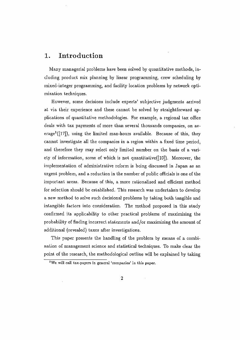
1. Introduction

Ma.ny ma.na.gerial problems have been solved by quantitative methods, in­

cluding product. mix planning by linear programming, crew scheduling by

mixed-integer programming, and facility location problems by network opti­

mization techniques.

However, some decisions include experts' subjective judgments arrived

at via their experience and these cannot be solved by straightforward ap­

plications of quantitative methodologies. For example, a regional tax office

deals with tax payments of more than several thousands companies, on av­

erage1([17]), using the limited man-hours available. Because of this, they

cannot investigate all the companies in a region within a fixed time period,

and therefore they may select only limited number on the basis of a vari­

ety of information, some of which is not quantitative([lO]). Moreover, the

implementation of administrative reform is being discussed in Japan as an

urgent. problem, and a. reduction in the number of public officials is one of the

import.a.nt a.reas. Because of this, a. more rationalized and efficient method

for select.ion should be established. This research was undertaken to develop

a new method to solve such decisional problems by taking both tangible and

intangible factors into consideration. The method proposed in this study

confirmed it.s applicability to other practical problems of maximizing the

probability of finding incorrect statements and/or maximizing the amount of

additional (revealed) taxes after investigations.

This pa.per presents the handling of the problem by means of a combi­

nation of management science and statistical techniques. To make clear the

point of the research, the methodological outline will be explained by taking

1 We will call tax-payers in general 'companies' in this paper.

2

t.he case of tax offices' investigations.

First, we construct an Analytic Hierarchy Process (AHP) model which

deals with both qualitative (intangible) and quantitative factors, in order to

rank the priority of companies. Then, we develop a stochastic model which

incorporates an AHP score with other related factors, in order to increase

probability of finding incorrectness. Actually, this process can be executed

by estimating the coefficients of the employed regression factors, using a past

data set; under a maximum likelihood rule. After the validity of this stochas­

tic model was confirmed, it can be used for the purpose of forecasting the

probability of finding an incorrect statement for each company. Finally, the

tax official scheduling problem will be solved via a 0-1 integer programming

model, along with the objective of maximizing the total probability or maxi­

mizing the total additional taxes, so that we can obtain a feasible and optimal

official schedule during a given time period.

The rest of the paper is organized as follows. Section 2 summarizes the

methodological issues. Section 3 deals with the construction of a stochastic

model which incorporates an AHP score with other related factors of impor­

t.a.nee. Then, in Section 4, the results thus obtained are used to construct

an optimization model for tax official scheduling within their limited capac­

ity. This process ensures the feasibility of the proposed method. Finally, in

Section 5, this process is applied to a Post-Clearance Audit Department of

Japanese Customs. A data set for the year of 1993 was employed to estimate

the corresponding stochastic model. After confirming the validity of such a

model, we then computed the probability for each importer (company) which

was utilized in the optimization model for scheduling of the officials. It was

found in this study that the probability of finding incorrect declarations is

theoretically improved from the present 60% to 75-80%0. Thus, this method

3

provides us with a.n optima.I strategy for the identification of incorrect tax

clecla.ra.tions. Although we applied this model to a. customs problem, there

are ma.ny other areas of interest to which it ca.n be successfully applied.

2. Methodological Outline

As was explained in the preceding section, one of the main objectives of

this research is to rank companies under investigation based on the likelihood

of incorrect declarations. Our judgment will be performed on the basis of

several criteria .. Some criteria are subjective and intangible. For this purpose,

we use the Analytic Hierarchy Process (AHP} first developed by Saaty([14]}.

Before going into the details of the AHP in our case, we will explain the

reason why we chose it from among other multiple-criteria decision ma.king

methodologies. As was mentioned in Belton[2], the field of multiple-criteria.

decision making (MCDM) has expanded rapidly over the last two decades and

continues to do so. Among the MCDM methodologies, the Multi-Attribute

Utility (or Va.Jue} Theory (MAUT[ll]} and the AHP a.re the approaches best

suit.eel for this kind of problem a.nd the most widely used in practice. (See

Belton[2].) Also, the review by Zanakis et al.(21] showed that these two have

been most frequently employed as the models for measurement within the

service a.nd government sectors. Ha.rker[9] compared the AHP with other

decision methodologies, especially with the Delphi technique and the MAUT

a.nd we agree with his views. The reasons for evaluating the AHP over the

MA UT a.re as follows: ( 1} We ca.n easily incorporate the hierarchy structure

of decision making problems into the AHP model. (2) We do not need any

assumption on a von Neumann-Morgentern type utility function estimation.

(3) We can evaluate the inconsistency of the decision maker. ( 4} The AHP

4

is fitted for group decision situations. And lastly, (5) the ARP can easily be

understood a.nd handled by practitioners.

However, the ARP has not been commonly accepted as an established

methodology and has been under active research a.nd development. It has

been criticized for its theoretical or axiomatic foundation. (See Belton and

Gea.r[3], for example.) Therefore, its users need to be careful in applying it

to their problems. In our case, as can be seen in Sections 3 a.nd 5, we do test

the statistical hypothesis on the relationship between the model scores and

the past data., where the model scores are obtained by combining the ARP

weights with other tangible factors. Thus, we can be, to some extent, free

from the criticisms occasionally showered on the AHP results.

Figure 1 describes a typical hiera.rchy structure for the ranking process

of selecting companies, which was constructed based on the publication in

reference to the investigations by Japanese tax offices ([10]).

Figure 1

5

The purpose of this AHP application is the selection of companies, as

indicated at the top of the hierarchy. The second level (criteria) consists

of such factors as Information, Interval of Investigation, Type of Business,

Contents of Declaration, and so forth. Finally, the third level comprises a

list of companies. It is important to note that this figure is shown only for

explanation of the method and does not reflect the hierarchy structure of

the case study of Section 5. The contents of the criteria should be selected

adaptively through expert opinion and experience of the problem. These

may vary according to time and place.

One of difficulties in applying the AHP method to our problem is the

'large' number of alternatives (companies), as depicted at the bottom level of

t.he hiera.rchy. Because of this, the number of pairwise comparisons becomes

too large to handle. For such cases, there are several expedients, some of

which can be summarized as follows:

1. Similar companies are classified into a reasonable number, (for example,

less than 9 groups), and they a.re compared pairwise with each other

with respect to the criteria in the upper level. This article refers to this

as 'grouping'.

2. For ea.ch criterion, we evaluate companies at the bottom by an absolute

measure(, e.g. 1 to 10 points), and obtain the score of the company as a

weighted sum of the absolute measures, where the weight is associated

with that of the criterion in the upper level. In this case, we need no

pairwise comparisons between companies. This article calls this pro­

cess, which was first developed by Saaty[15], 'absolute measurement'.

3. Harker[8] describes a set of techniques to reduce the number of pairwise

comparisons that the decision maker must make during the analysis of

6

a large hierarchy. We can apply his 'incomplete' pairwise comparison

technique. Tone[18] discussed a similar reduction technique within the

framework of the geometric mean method.

4. Weiss and Rao[l9] proposed the use of incomplete experimental designs,

e.g., the method of balanced incomplete block designs (BIBD), for sim­

plifying the data-collection tasks. This method reduces the number of

pairwise comparisons, while still ensuring that every pair of attributes

is replicated the same number of times in the design.

We can choose one of these expedients according to the situations of the

companies. There are several variants in the absolute measure with regard

to the range of points, e.g. a 5 point measure, a 7 point measure. The results

and conclusions may differ according to the range. The choice depends largely

on practitioners' experiences in the decision is.sue. In some cases, they may

think t.ha.t a. 5 point system is enough for the problem. Another recourse is

to choose t.he points measure that gives the highest fitness in the stochastic

model described in Section 3.

The next step is to check the fitness of the AHP score to the actual

findings of incorrect statements. This process can be carried out using a

past data. set. If both incorrect (false) statements were found in companies

with high AHP scores and the relationship between incorrect statements and

AHP scores was proved to be statistically significant, then we could utilize

the AHP results for selection of future investigations. At this stage, this

study will employ not only the AHP scores but also other considerable re­

lated factors, (e.g. annual turnover, annual profit, annual profit/employee,

capital, the number of employees and so forth), all of which are quantita­

tive, not included in the AHP criteria, and are judged to be significant for

7

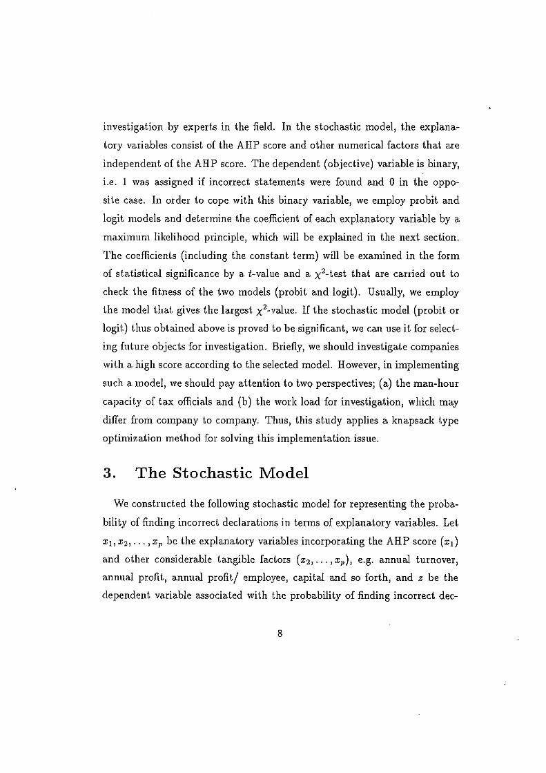
investiga.tion by expert.s in the field. In the stochastic model, the explana­

tory variables consist of the AHP score and other numerical factors that are

independent of the AHP score. The dependent (objective) variable is binary,

i.e. 1 was assigned if incorrect statements were found and 0 in the oppo­

site case. In order to cope with this binary variable, we employ probit and

logit models and determine the coefficient of each explanatory variable by a

ma.ximum likelihood principle, which will be explained in the next section.

The coefficients (including the constant term) will be examined in the form

of statistica.l significa.nce by a. t-value and a x2-test that are carried out to

check the fitness of the two models (probit and logit). Usually, we employ

the model that gives the largest x2-value. If the stochastic model (probit or

logit.) thus obtained a.hove is proved to be significant, we can use it for select­

ing future objects for investigation. Briefly, we should investigate companies

with a high score according to the selected model. However, in implementing

such a. model, we should pay attention to two perspectives; (a) the man-hour

capacity of tax officials and (b) the work load for investigation, which may

differ from company to company. Thus, this study applies a knapsack type

optimization method for solving this implementation issue.

3. The Stochastic Model

We constructed t.he following stochastic model for representing the proba­

bility of finding incorrect declarations in terms of explanatory va.riables. Let

x1, x2, ... , Xp be the explanatory variables incorporating the AHP score (x1)

and other considerable tangible factors (x 2 , .•. , xp), e.g. annual turnover,

annual profit, annual profit/ employee, capital and so forth, and z be the

dependent variable associated with the probability of finding incorrect dee-

8

la.rations. This study assumes the following model:

(1)

where c: is a random error term.

In order to estimate the coefficients f3; (j = 0, ... , p), this study uses past

data concerning n investigations:

(x1i, X2i 1 • • ·, Xpi, Yi), (i = 1, ... , n) (2)

where Yi is binary, i.e. Yi = 1 when incorrect statements found and y; = 0 for

otherwise.

As an expected correspondence between z and y, we assume that if z > 0,

then y = 1 and if z :::; 0, then y = 0.

Let F be the cumulative distribution of the random variable z. Then, the

probability of y; = 1 is given by

(3)

where z; = (30 + f31x1; + · · · + (JpXpi·

The relationship between z and y needs some attention. Suppose that we

assume z = y and apply the stochastic model below to the data (2).

(4)

Then, we can find the coefficient ((30, f3;, ... , f3;) by the least squares prin­

ciple. This is a computationally simple method. However, in this case, the

model value calculated by

(5)

9

does not necessarily satisfy the relationship

(6)

This condit.ion is definitely necessary to interpret Y; as probability. Even if

we further impose the condition (6) in estimating the coefficient, the param­

et.ers in the model ( 4) inevitably have a limited interpretation and range of

validity. Furthermore, this type of straight application of the least squares to

binary data has several statistical drawbacks with respect to the fundamen­

tal assumptions underlying the least squares, since the dependent variable y;

takes only the values 0 and 1. (See Cox[5] pp.16-18, in detail.) Therefore,

we need a type of model in which the constraint (6) is automatically satis­

fied. In many respects, the simplest way of representing the dependence of a

probabilit.y on explanatory variables so that the constraint ( 6) is inevitably

satisfied, is to postulate a dependence for i = 1, · · ·, n,

P(y; = l) = exp(z;) , 1 + exp(z;)

(7)

where z; = /30 + f31 x1; + · · · + (JpXp;· This model is called the linear logistic

model or the logit model.

Another candidate is the standard normal distribution which is expressed

as

jz; . 1 2

P(y; = 1) = -e-"' i2 dx. -oo vz; (8)

this model is called the probit model.

(The following statistical areas are discussed in detail in [1], [5], [13] and

[16], in the reference list.)

10

3.1. Logit and Probit Models

As mentioned above, this study employs two models; logit and probit, for

expressing t.he cumulative distribution F, since they are representative of the

latent. trait. for dealing with binary random variables.

1. Logit Model

In this case, F is the cumulative distribution of a logistic distribution

and is expressed as: e'

A(z)- -­- 1 + e''

Thus, the probability of Yi = 1 becomes

2. Probit Model

(9)

F is the cumulative distribution of the standard normal distribution

which is expressed as:

<f>(z) = j' _l_e-x'f2dx. -oo vz; ( 10)

The probability of Yi = 1 is expressed by

3.2. Estimation of Coefficients

We estimated the coefficient (/30, ... , /3p) of these models using past data

sets (x 1;, ... , Xp;, Yi) (i = 1, ... , n). For this purpose, the following likelihood

function is fully utilized:

L(/30, ... , /3p) = IT F(zi) x II [1 - F(zi)], (11) y;=O Yi=l

11

where z; = /30 + /31xli + · · · + /3pxp;. The logarithmiclikelihood function, log L,

is maximized in (/30, ... , /3p)· This task requires solving (p + 1) simultaneous

nonlinear equations in the (p + 1) unknown parameters.

There are numerous procedures for finding numerically the maximum of a

relatively complicated function like (11). Usually, the Newton-Raphson iter­

ative solut.ion (Fletcher (7]) of the maximum likelihood equation is effective,

especially if the number of parameters is not so large.

3.3. The Standard Error of Esti1nated Coefficients

Let the column vector :v; be (1, x 1;, ... , Xp;JT, /3 be the maximum likelihood

estimation of /3 = (/30, · · ·, /3p)T and J(z) be the probability density function

of F. Then, if the number of data approaches infinity, the distribution of

fo(/3- /3) comes to display the multivariate normal distribution N(O, B-1 ),

where the (p + 1) x (p + 1) matrix Bis defined by

. 1 ~ J2(:vT /3) T B = hm - L., F( T/3)( F( T/3)) :V;:V; . n-+oo n. . { ~. 1 - f "' • t=l ..... , ..... ,

In the case of a large enough n, this term can be approximated by

' 1 ~ j2(z;) T

B =; f;r F(z;)(l - F(z;)) :V;:V;'

where z; is the model value for (x 1;, ... , xP;).

(12)

(13)

From the results of the above definitions, the square root of the diagonal '-1

elements of B gives the standard deviation for each estimated coefficient.

Moreover, this research tests the significance of the coefficients by their t­

values.

12

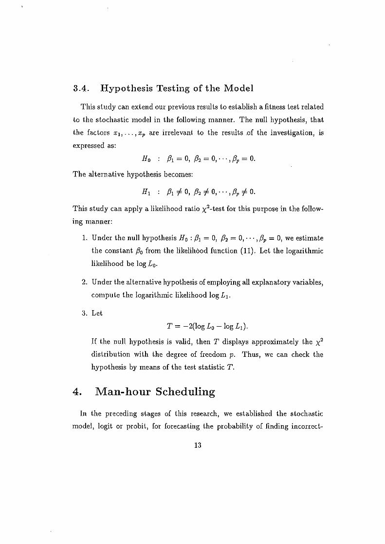
3.4. Hypothesis Testing of the Model

This study can extend our previous results to establish a fitness test related

to the stochastic model in the following manner. The null hypothesis, that

the factors X1i ••• , Xp are irrelevant to the results .of the investigation, is

expressed as:

Ho : /31 = O, /32 = 0, · · · , /3p = 0.

The alternative hypothesis becomes:

This study can apply a likelihood ratio x2-test for this purpose in the follow-

mg manner:

1. Under the null hypothesis Ho : /31 = 0, /32 = 0, · · ·, /3p = 0, we estimate

t.he constant /30 from the likelihood function (11). Let the logarithmic

likelihood be log L0 .

2. Under the alternative hypothesis of employing all explanatory variables,

compute the logarithmic likelihood log L1 .

3. Let

T = -2(log Lo - log L1).

If the null hypothesis is valid, then T displays approximately I.he x2

distribution with the degree of freedom p. Thus, we can check the

hypothesis by means of the test statistic T.

4. Man-hour Scheduling

In the preceding stages of this research, we established the stochastic

model, logit or probit, for forecasting the probability of finding incorrect-

13

ness, 1.e.

or

depending upon the model chosen for our investigation.

Let Pi be the probability of the j-th candidate company (j = 1, ... , l)

which is calculated by the above formula.

At this stage, we need to consider several factors for implementing our

search procedure. One is the work load for investigation, which may differ

from company to company, and the others are the limit of available man­

hours for investigation and the upper limit of number of companies to be

investigated for a given time period.

Let di (j = 1, ... , l) be the work load (man-hour) for the j-th company, D

be the total available man-hours and N be the upper limit of investigations.

Officials can determine the work load di by considering such factors as the

sea.le and the variety of information of the company j and so on. Then, we

have the following knapsack type problem:

I

max w - LPizi j=l

I

subject to "L, djZj < D j=J

I

LZj :::; N, Zj E {O, 1}. i=l

(14)

(15)

(16)

The objective is to find the opt.imal assignment of officials so that it max­

imizes the sum of the probability of finding incorrectness under the total

man-hours and the upper limit constraints.

14

The above model has several variants, among which we will select a sim­

ple but important one with multi-resource constraints. The objective is to

maximize the expected total additional tax.

I

max w - I:, Pi a1 Zj j=I

I

subject to I:, djkZj < Dk (k = 1, ... , K) j=I

I

I:, Zj :::; N, Zj E {O, 1}, j=l

(17)

(18)

(19)

where a1 is the expected additional tax paid by the j-th company, djk is the

work load of resource k for investigating company j, and Dk (k = 1, ... , K)

is the limit of the available amount of resource k. We can solve these models

by using software for linear programming problems with 0-1 integer variables.

5. A Case Study

In this section, the applicability of the proposed method is verified by a

case study. The subject chosen is a. selection problem of importers to be

investigated by a Post-Clearance Audit Department of Japanese Customs.

Before going into a detailed analysis, we will describe briefly the Customs

investigation system in Japan. Genera.Uy, the Customs employs the post­

clea.ra.nce audit system based on the self-assessment made by importers. Then

Customs officials examine the documents in order to confirm whether the

declared value was right or not after clearance. If incorrect declarations

a.re found as a result of investigation, officials usuaily recommend importers

to correct their declarations. However, in cases where officials judge the

false declaration was made intentionaily, importers would be punished via

15

Customs Law and so on.

Practically, because of limited man-hours, they cannot investigate all im­

porters, and the Customs selects companies based on their experience and a

variety of information. It is reported that the rate of finding incorrect. dec­

la.ra.tions is approximately 60% and this percentage has remained same for

the past several years ([6]). It is therefore considered to be a.n urgent subject

for the Customs to develop a more efficient selection methodology for this

purpose.

The following case study utilizes the Customs data of the year 1993 to

build up the proposed stochastic model and the scheduling model of officials.

Then, we applied the models thus obtained for the data of 1994. The com­

panies under investigation are classified into three categories denoted as A,

B and C, depending on their type of industry.

This section is divided into three parts. In Section 5.1, we select a small

data set in Category A from the 1993 data and follow the proposed method

step by step so that the numerical treatments can be better understood.

Then, in Section 5.2, the whole data set is analyzed. It was found that the

probability of finding incorrect declarations can be improved from the present

60% to 75-80%. Lastly, in Section 5.3 some observations will be presented

on why this improvement was made possible by our proposed method.

5.1. A S111all Data Set Case

Although this study utilizes the whole data set kept by Yokohama Customs,

it is impossible to describe the numerical treatments in detail. Therefore, we

trace the calculation processes in the case of a limited number of data. For

this purpose, the data of twenty three companies (Tl to T23) in Category A

were chosen. The 23 companies were further divided into 4 groups according

16

to their imported materials. The number of samples are six each for Group

1 to Group 3 and five for Group 4. (See Table 5.)

5.1.1 Subjective Judgment by AHP

The hierarchy structure in the AHP model was established by experts'

opinions (Figure 2). The structure is conceptually similar to Figure 1. A

part of the pairwise comparisons and AHP scores for Group 1 (Tl to T6) are

shown in Tables 1 to 4. (Those for other groups are not shown.). It should be

not.ed t.hat t.he AHP scores of Group 4 are multiplied by 5/6, since this group

contains 5 companies while others contain 6. Thus, the summation of scores

in this group is 5/6. (See Table 5.) We call this operation normalization. The

AHP scores of 23 companies thus obtained are exhibited in AHP column in

Table 5.

Figure 2

Table 1 to Table 4

5.1.2 Construction of Stochastic Model

In addition to the AHP scores, the proposed method deals with other tangi­

ble factors, such as annual turnover, profit, capital, and number of employees

17

in t.he company. We examined the correlation analyses between the probabil­

ity of finding incorrect declarations and each tangible factor and found that

an index which represents the scale of foreign trade is significantly correlated.

After these preliminary surveys with the intangible (AHP) factor and

t.he tangible factor (scale of foreign trade), we developed the logit and the

probit. models, including two explanatory variables, expressed by AH P and

x. Accordingly, t.he mathematical expression becomes

(20)

The coefficients (30 , (31 and (32 are estimated by utilizing 23 sets of data shown

in Table 5, where the column Yi takes the value 1, if incorrect declarations

are found, and 0 otherwise.

Table 5

By using the maximum likelihood estimation, the following model equa­

tions were obtained. Standard deviation, t-value and x2-value for each coef­

ficients are shown in Table 6.

Logit Model

z = -4.460 + 21.81AH P + 8.468 x 10-3x + <. (21)

Probit Model

z = -2.543 + ll.89AH P + 4.973 x 10-3 x + t. (22)

18

Table 6

Although the logit model has a. larger x2-value as shown in Table 6, we

chose the probit model, since the latter has slightly larger t-value for all three

coefficients. 2

We now consider a knapsack type 0-1 integer programming problem cor­

responding to the expressions (14) to (16) in Section 4. The coefficient P; in

the objective function is estimated through the Logit model (21) as described

in Section 3. Since the demonstration of this small sample is purely for ex­

planatory purposes, the work load d; is chosen randomly from the interval

[4, 12], and we set D (the total man-hours available) = 40 and N (the upper

limit of investigations) = 9. See Table 7.

By using the software XPRESS -MP ([20]), we obtained the optimal so­

lution {zi} as exhibited in Table 7, where zi = 1 means 'to go' and zi = 0

'not to go'. Eventually, this optimal solution chose companies with a high

p; value, and eight .out of nine companies investigated were found to have

declared incorrectly. Since the purpose of this part of the case study is to

demonstrate the proposed processes, we do not intend to compare the opti­

mal solution with the actual investigation results.

Table 7

2It is reported that there is, in most cases, no significant difference between the probit and the legit models in binary data analysis ([16]).

19

5.2. Results Obtained Using the Whole Data

Yokohama Customs investigated several hundreds of importers in 1993.

Estimation of the coefficients, /30 , /31 and /32 , was carried out using the data

set3 for 1993, of which a portion is exhibited in Table 8. Table 9 presents

the results along with the t-value for each estimated coefficient and the x2-

value for each model. All the coefficients and both models were found to be

statistically significant.

I Table 8

Furthermore, Table 10 shows the correlation coefficient between the model

and the actual value for each category. More exactly, these coefficients were

calculated as follows. Suppose that the i-th importer in category A has the

model value z;, and the actual probability of finding incorrectness in the

class to which the importer belongs is z;. The class was determined by a

level of the AHP score and one tangible factor. The correlation coefficient

was calculated as the one between {(z;, z;)}(i E Category A). Again, all

coefficients were found to be statistically significant. Here, we chose the one

with both a larger x2 value and coefficients of correlation in this case.

3Due to the confidential nature of the subject matter, we cannot disclose actual data employed.

20

Table 9

Table 10

Then the numerical computations of a knapsack type 0-1 integer pro­

gram were performed with a data set for the year 1994 in three categories of

importers, under several varieties of constraints regarding the available man­

hours and the upper limit of investigations. We obtained approximately 80%

as t.he a.verage of these forecast.ed probabilities of selected importers, i.e.,

those of companies with z; = 1. Consequently, if we implement our cus­

toms investigation based on the optimal solution { zi}, the probability of

identifying incorrect declarations may be increased from the present 60% to

80%.

5.3. So111e Observations on the Case Study

This study applied our method to the data set of Yokohama Customs in

the year of 1993 and 1994. More concretely, first; the 1993 year data were

utilized to establish the stochastic models and then the models were applied

to forecast the probability of finding incorrect declarations of companies for

the year 1994. Based on the probability thus estimated, the 0 - 1 integer

linear program was solved optimally to determine which companies should be

21

investigated within the available man-hours and the upper limit constraints.

The results indicate that the probability of finding incorrect declarations

could be raised from the present 60% to 803, at least theoretically. This is

a remarkable difference and improvement.

We believe this improvement was caused by the combination of experts

knowledge and management science methodologies. From long experience,

the expert officials know which factors a.re important in determining where to

investigate. However, these factors would be mostly intangible and difficult to

prioritize. The AHP succeeded in measuring the priorities of these intangible

factors and in scoring the incorrectness of target companies. Furthermore,

the stochastic model, which combines the AHP score with other tangible

factors, had its creditability verified by statistical tests. The improvement

is the result of deliberate integration of expert knowledge and management

science methodologies.

6. Conclusion

This article proposed a new search model with subjective judgments and

then applied it. to the selection work of the Post-Clearance Audit Department

of Japanese Customs. It. found that the probability of finding incorrect dec­

la.ra.tions could be improved from the current 603 to 803. This improvement

is realized by the combination of wide expert knowledge and mathematical

methodology.

However, it should be noted that the data. set used in our experiment was

obtained from a conventional selection process (not by the proposed one) and

hence, if the Japanese Customs could replace its selection process by the one

proposed in this research, we expect that the rate of finding incorrectness

22

might be further improved. It is hoped that this model will be applied to

other similar kinds of administrative investigations and criminal inspections.

In this research, AHP scores were used together with logit and probit

models as suitable for forecasting the probability of finding incorrect customs

decla.ra.tions. Then, we solve a resource allocation problem for finding the

optimal assignment of tax officials, using the results of the stochastic model

as data.

Za.na.kis et al. [21] surveyed 306 articles on program evaluation and fund

allocation methods within the service and government sectors, which ap­

peared in 93 journals. They found that few publications dealt with evaluation

and allocation as an integrated process. Actually, in only two, ( Bodily[4]

and Khorra.mshahgol and Steiner[12]), were such approaches within criminal

and law enforcement applications. Our approaches are different from theirs

in following ways. The former deals with the spatial design problem of the

police mobile units, incorporating the multi-objectives of administrations,

citizens and service personnel. Using multi-attribute utility theory, alterna­

tive locations a.re evaluated according to the preferences for efficiency and

equality of service of the three interest groups. Iterative improvements and

heuristics are utilized to find a satisfactory solution. Bodily's paper is differ­

ent from ours in the problem area examined and methodologies employed.

It concerns a. stationary allocation problem, while ours deals with a search

model. The la.t ter paper by Khorra.mshahgol et al. deals with the problem

of allocating funds to competing projects. Investment decisions normally

involve several, often conflicting and non-commensurable, goals. So, they

applied the goal programming approach to this problem, where the weights

to the goals were determined by the Delphi method. Thus, this work dif­

fers from ours in methodology. Instead of the Delphi method, we utilized

23

the AHP results coupled with the stochastic model and tested its statistical

significance. (Saaty[14] described comparisons between the AHP and the

Delphi method.)

Thus, we believe and hope that this article will present a new methodology

for law enforcement and criminal applications.

Finally, as an important future research task, this study will extend our

interest t.o an investigation regarding which stochastic models will be appli­

cable to other decisional issues in both the public and private sectors.

Acknowledgment

The authors wish to thank two anonymous referees for their valuable sug­

gestions and the staff of Yokohama Customs for supporting the study.

References

[1] Amemiya, T., Advanced Econometrics, Harvard University Press, 1985.

[2] Belt.on, V., "A Comparison of the Analytic Hierarchy Process and a Sim­

ple Multi-Attribute Value Function,'' European Journal of Operational

Research, Vo.26, pp.7-21, 1986.

[3] Belton, V. and T. Gear, "On a Shortcoming of Saaty's Method of Ana­

lytic Hierarchies,'' Omega, Vol. 11, pp.228-230, 1984.

[4] Bodily, S.E., "Police Sector Design incorporating Preferences of Inter­

est Groups for Equality and Efficiency,'' Management Science, Vol. 24,

pp.1301-1313, 1978.

[5] Cox, D.R., Analysis of Binary Data, Methuen, 1970.

24

[6] Customs and Tariff Bureau, Ministry of Finance, Japanese Government,

The Third Annua.l Report of Customs and Tariff Bu.reau, Nippon Kanzei

Kyokai, 1994.

[7] Fletcher, R., Pra.ctica./ Methods of Optimization, Vol. 1, John Wiley &

Sons, 1980.

[8] Harker, P.T., "Incomplete Pairwise Comparisons in the Analytic Hier­

archy Process," Mathematical Modelling, Vol. 9, pp.837-848, 1987.

[9] Harker, P.T., "The Art and Science of Decision Making: The Analytic

Hierarchy Process," in The Analytic Hierarchy Process, B.L. Golden,

E.A. Wasil and P.T. Harker (Eds.), Springer-Verlag, pp.3-36, 1989.

[10] Hotti, T., The Scene of the Tax Investigations by Tax Offices, Gyousei,

1995.

[11] Keeney, R.L. and H. Raiffa, Decision with Multiple Objectives: Prefer­

ence a.nd Valu.e Tradeoffs, John Wiley, New York, New York, 1976.

[12] Khorramshahgol R. and H.M. Steiner, "Resource Analysis in Project

Evaluation: A Multicriteria Approach,'' J. of Operl. Res. Soc., Vol. 39,

pp. 795-803, 1988.

[13] Pindyck, R.S. and D.L. Rubinfeld, Econometric Models and Economic

Forecasts, Second ed., McGraw-Hill, 1981.

[14] Saaty, T.L., The Analytic Hierarchy Process, McGraw-Hill, 1980.

[15] Saat.y, T.L., "Absolute and Relative Measurement with the AHP. The

Most Livable Cities in the United States," Socio-Eco. Plann. Sci. Vol.20,

No. 6, pp.327-331, 1986.

25

(16] Takeuchi, K. et al., Analysis of Scientific Data (Basic Statistics 3}, The

St.atistic Section, Department of" Social Science, College of Arts and

Science, University of Tokyo, University of Tokyo Press, 1992.

(17] Tax Agency, Japanese Government, The 120th Annual Statistical Report

of Tax Agency, Okura Zaimu Kyokai, 1994.

(18] Tone, K., "Two Technical Notes on the AHP Based on Geometric Mean

Method,'' in Proceedings of the Fourth International Symposium on the

Analytic Hiera.rchy Process, Faculty of Business Administration, Simon

Fraser University, Canada, pp.375-381, 1996.

(19] Weiss, E.N. and V.R. Rao, "AHP Design Issues for Large-Scale Sys­

tems,'' Decision Sciences, Vol. 18, No. 1, pp.43-61, 1987.

(20] XPRESS-MP, Release 7, Dash Associates.

(21] Zanakis, S.H., T. Mandakovic, S.I<. Gupta, S. Sahay and S. Hong, "A

Review of Program Evaluation and Fund Allocation Methods Within

t.he Service and Government Sectors," Socio-Eco. Fiann. Sci. Vol.29,

No.l, pp.59-79, 1995.

26

Selecting Companies ;

Information Interval of Type of Contents of Investigation Business Declaration

a b c d e f g

Fig. 1. Hierarchy Structure for Selecting Companies

Selecting Imwrtcrs

Al A2 A3 A4 A5

A6 A7

Tl T2 T3 T4 T5 T6

Fig.2. Hierarchy Structure for Selecting Importers

Table I. Pairwise Comparisons of Selecting Importers

Al Al l AZ 6 A3 3 A4 1/4 AS 7

Table 3. I.

Al Tl Tl 1 T2 z T3 1/7 T4 1/6 TS 1/9 T6 1/7

Table 3. 2.

AZ Tl Tl l TZ l/S T3 2 T4 1 TS 1/3 T6 3

AZ A3 A4 AS weight 1/6 1/3 4 1/7 o. 0697 l z 6 1/3 o. Z41Z

l/Z l 3 1/7 o. 118Z ;

1/6 1/3 1 1/8 o. 0374 3 7 8 1 o. S336

C. I. =O. 09S C. R. =O. OBS

Table2. Pairwise Comparisons of A3

A3 A6 A7 weight A6 1 s 0.8333 A7 l/S 1 o. 1667

C. I. =O. 000 C.R. =O. 000

Pairwise Comparisons of Al

T2 T3 T4 TS T6 weight 1/2 7 6 9 7 o. 3264 l 8 7 9 8 o. 4431

1/8 l 1/2 s 1 o. OS80 1/7 2 l 7 2 o. 0923 119 l/S 1/7 1 l/S o. 0223 1/8 1 l/Z s 1 o. OS80

C. I. =O. 09S C.R. =O. 077

Pairwise Comparisons of A2

TZ T3 T4 s 1/2 l 1 1/7 l/S 7 1 z s l/Z 1 3 1/4 1/3 8 z 3

TS T6 weight 3 1/3 o. 1442

1/3 1/8 o. 0313 4 l/Z o. 2419 3 1/3 o. 144Z 1 l/S o. 0636 s l o. 3748

C. I. =O. 023 C.R. =O. 019

Table 4. Results of AHP

AHP score Tl o. Z470 T2 O. 1S81 T3 O. 2628 T4 O. 09S3 TS 0. 07S6 T6 O. 1610

Table 5. Small Sample Data for Estimating Coefficients

i con1pany group AHP foreign trade ' detection

AHP; X; Y; 1 Tl 0.247 562.58 1 2 T2 0.158 455.90 1 3 T3 1 0.263 92.49 1 4 T4 0.095 55.96 0 5 T5 0.076 6.91 0 G T6 0.161 15.09 1 7 T7 0.128 407.9 1 8 TS 0.298 44.22 1 9 T9 2 0.161 24.08 0

10 T10 0.289 34.44 1 11 Tl 1 0.060 51.49 0 12 T12 0.063 50.59 0 13 T13 0.225 475.63 1 14 T14 0.139 92.82 0 15 T15 3 0.184 52.00 1 1 G Tl 6 0.241 547.12 1 17 T17 0.136 556.19 1 18 Tl 8 0.075 49.17 0 19 T19 0.217 25.78 1 20 T20 0.188 658.10 1 21 T21 4 0.285 128.35 0 22 T22 0.072 26.87 0 23 T23 0.072 22.41 0

* y; = 1, if incorrect declarations found,= 0 if not found.

Table 6. Results of Statistical Tests

/3 0 /31 /3 2

Model t-value t-value t-value x '-value level level level level

Logit -2. 354 2. 135 1. 645 17. 08 5% 5% 20% 1%

Probit -2. 665 2. 381 1. 900 17. 01 5% 5% 10% 1%

* level means significant level.

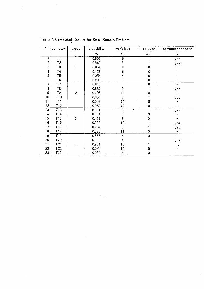
Table 7. Computed Results for Small Sample Problem

i con1pany group probability work load solution correspondence to

d; • P; Z; Y; 1 Tl 0.999 6 1 yes 2 T2 0.945 5 1 yes 3 T3 1 0.852 9 0 -4 T4 0.128 6 0 -5 TS 0.054 4 0 -6 T6 0.290 7 0 -7 T7 0.843 4 0 -8 TB 0.887 9 1 yes 9 T9 2 0.305 10 0 -

10 T10 0.856 8 1 yes 11 Tl 1 0.058 10 0 -

12 Tl 2 0.062 12 0 -13 T13 0.994 6 1 yes 14 T14 0.334 8 0 -15 T15 3 0.461 8 0 -16 Tl 6 0.999 12 1 yes 17 Tl 7 0.967 7 1 yes 18 Tl 8 0.080 11 0 -19 T19 0.565 5 0 -20 T20 0.998 4 1 yes 21 T21 4 0.931 10 1 no 22 T22 0.060 12 0 -23 T23 0.058 4 0 -

Table 8. Past Data Set for Estimating Coefficients

Importer 1, 1, /3 ..... I n-1 In Category Factor

AHP 0.095 0.177 0.139 ..... 0.104 0.307 A x 55.96 446.8 2835 ..... 41.19 105.7

v 0 0 1 ..... 0 1 AHP 0.209 0.198 0.270 ..... 0.243 0.085

B x 45.23 10.30 125.1 ..... 678.1 5.909 v 0 1 1 ..... 1 0

AHP 0.125 0.191 0.264 ..... 0.074 0.072 G x 70.44 61.75 184.5 ..... 20.82 9.537

y 0 1 1 ..... 1 0

* n is different for each category

Table 9. Results of Coefficients Estimation and Statistical Tests

f3 0 {3 I f3 2 x 2-value Category Model (t-value) Ct-value) ( t-value) (level)

(level) (level) (level)

Prob it -1.450 6.051 7.631 x 10-3 25.486 (-3.805) (3.213) (2.850) (1 %)

A ------------ _J] _____ ~)__ __(L_J!L ___ J] _____ ~) _____ L------------·

Lo git -2.559 10.71 4.666 x 10-2 26.411 (-3.787) (3.223) (2.898) (1 %) (1 %) (1 %) (1 %)

Prob it -1.124 4.155 8.177 x 10-3 16.770 (-2.948) (2.107) (2.568) (1 %)

B _J] _____ ~) __ __ (q__ ___ ~L_ (5 %) ------------ --;:428_;_1_0:;-- ------------· Lo git -1.948 7.152 17.123

(-2.972) (2.150) (2.441) (1 %) (1 %) (5 %) (5 %)

Prob it -1.230 4.641 9.593 x 10-3 12.680 (-2.825) (2.041) (2.042) (1 %)

G _J] _____ ~) __ c __ (t __ J!L _ __ J? _____ ~) _____ ------------ ------------· Lo git -1.995 7.449 1.578 x 10-2 12.480

(-2.972) (1.946) (1.894) (1 %) (1 %) (10 %) (10 %)

* model: z = f3 0+ f3 1 AHP+ f3 2x+ e

Table 10. Correlation Coefficients between Model and Data

Category Model correlation level A Prob it 0.8751 1%

Lo•it 0.8628 5% B Prob it 0.9060 1%

Lo•it 0.9169 1% G Prob it 0.9509 1%

Lo git 0.9465 1%