1

A Scalable Application Placement Controller for Enterprise Data Centers

Chunqiang Tang, Malgorzata Steinder, Michael Spreitzer, Giovanni Pacifici

IBM T.J. Watson Research Center19 Skyline Drive, Hawthorne, NY 10532, USA

fctang, steinder, mspeitz, giovannig@us.ibm.com

2007 WWW

2

Outline

• Introduction• Problem Formulation• The Placement Algorithm• Experimental Results• Conclusion• Comment

3

Introduction

• With the rapid growth of the Internet, many organizations increasingly rely on Web applications to deliver critical services to their customers and partners

• The Web request rate is bursty and can fluctuate dramatically in a short period of time .– it is not cost-effective to over provision data centers to handle the

potential peak demands of all the applications.

• Web applications typically run on top of a middleware system – Use clustering technology

4

Clustered Web ApplicationsThe request router may implement functions such as admission control, flow control, and load balancing.

request rate for application z suddenly surges

5

Dynamic Application Placement

「Given a set of machines with constrained resources and a set of Web applications with dynamically changing demands, how many instances to run for each application and where to put them?」－ Dynamic application placement

• The application placement problem can be formulated as a variant of the Class Constrained Multiple-Knapsack Problem– Under multiple resource constraints (e.g., CPU and memory)

application constraints (e.g., the need for special hardware or software)

6

Control Loop

Periodically every T minutes, produces a new placement solution (e.g., T=15 minutes)

7

Estimating Application Demands

• Estimating application demands is a non-trivial task. – online profiling and data regression to dynamically estimate the

average CPU cycles needed to process one Web request of a given application [11].

• A running application instance's consumption of CPU cycles and IO bandwidth depends on the request rate.

• For memory, our system periodically and conservatively estimates the upper limit of an application's near-term memory usage

[11] G. Pacici, W. Segmuller, M. Spreitzer, and A. Tantawi. Dynamic Estimation of CPU Demand of Web Tracffic. In Proceedings of the First International Conference on Performance Evaluation Methodologies and Tools (VALUETOOLS), 2006.

8

Upper Limit of Memory

• Use the conservatively estimated upper limit for memory consumption– a significant amount of memory is consumed even if it receives no

requests– memory consumption is often related to prior application– many applications cannot run when the system is out of memory

• Among many resources, we choose CPU and memory as the representative ones to be considered– Network bandwidth

9

Problem Formulation

• The placement controller strives to find a placement solution that – maximizes the total satisfied application demand– minimizes the total number of application starts and stops– balance the load across machines(the utilization of individual machines should stay close to the utilization p of the entire system)

Problem Formulation

10

the utilization p of the entire system:

(Let I* denote the old placement matrix, and I denote the new placement matrix)

11

The Placement Algorithm

• Our algorithm repeatedly and incrementally optimizes the placement solution in multiple rounds– In each round, it first computes the maximum total application

demand that can be satisfied by the current placement solution

• it shifts load across machines (without placement changes)

• stopping unproductive application instances and starting more useful ones in order to increase the total satisfied application demand(placement change)

12

Definition of Terms• A machine is fully utilized if its residual CPU capacity is zero

– (Ω*n = 0)

otherwise, it is underutilized.

• An application instance – is fully utilized if it runs on a fully utilized machine.– An instance of application m running on an underutilized machine n is

completely idle if it has no load (Lm,n=0)– otherwise, it is underutilized.

• The load of an underutilized instance of application m can be increased, if application m has a positive residual CPU demand(ω*m>0)

13

Definition of Terms

• The CPU-memory ratio of a machine n is defined as its CPU capacity divided by its memory capacity(Ωn/Γn).– it is harder to fully utilize the CPU of machines with a high CPU-

memory ratio. • The load-memory ratio of an instance of application m

running on machine n is defined as the CPU load of this instance divided by its memory consumption (Lm,n /γm).– application instances with a higher load-memory ratio are

more productive.

14

The Placement Algorithm

15

Key Ideas in Load Shifting

• The running instances of an application into three categories:– Idle -> shut down– Underutilized– fully utilized –> do not change

• After load shifting, every application has at most one underutilized instance in the entire system– Because the strategy to handle idle instances and fully

utilized instances are straightforward

16

Key Ideas in Load Shifting

• Strive to co-locate residual memory and residual CPU on the same machines – these resources can be used to start new application

instances

• Strive to make idle application instances appear on machines with relatively more residual memory– By shutting down the idle instances, more memory will

become available for hosting applications that require a large amount of memory

17

The Load Shifting Subroutine• Given the current application demands, the placement

algorithm solves a max-flow problem [2] to derive the maximum total demand that can be satisfied by the current placement matrix I.

the capacity of this link is the CPU demand of the application (ωm)

the capacity of this link is the CPU capacity of the machine (Ωn)

Sort all the machines in increasing order of residual memory capacity Γn

[2]R. K. Ahuja, T. L. Magnanti, and J. B. Orlin, editors. Network Flows: Theory, Algorithms, and Applications. Prentice Hall, New Jersey, 1993. ISBN 1000499012.

18

The Load Shifting Subroutine

• The load distribution matrix L produced by solving the min-cost max-flow problem.

• the following good properties that make later placement changes easier:– (1) An application has at most one underutilized instance – (2) Residual memory and residual CPU are likely to co-

locate on the same set of machines.– (3) The idle application instances appear on the machines

with relatively more residual memory.

19

The Placement Algorithm

20

Key Ideas in Placement Changing

• The algorithm walks through the underutilized machines sequentially and makes placement changes to them one by one in an isolated fashion– only concerned with the sate of machine n and the residual

application demands

• The isolation of machines may lead to inferior placement solutions. – address this problem by alternately executing the load-shifting

subroutine and the placement-changing subroutine for multiple rounds

21

Key Ideas in Placement Changing

• The algorithm first considers machines with a relatively high CPU-memory ratio– is harder to fully utilize the CPU of these machines

• The algorithm tries to find a combination of applications that lead to the highest CPU utilization of this machine– stop “unproductive” running application instances with a relatively

low load-memory ratio to accommodate new application instances.

• To reduce placement changes, the algorithm does not allow stopping application instances that already deliver a “sufficiently high” load– refer to these instances as pinned instances

22

Before the Placement Changing

• Computes the residual CPU demand of each application. – We refer to the applications with a positive residual CPU demand

(residual applications)

• Inserts all the residual applications into a right-threaded AVL tree called residual app tree– sorted in decreasing order of residual demand

• Keeps track of the minimum memory requirement γmin of applications in the tree– a machine n's residual memory is smaller than γmin (this machine cannot accept any applications in the residual app tree)

23

The Placement Changing (Outermost Loop)

Change the placement on one machine at a time

24

The Outermost Loop

• Excludes fully utilized machines from the consideration of placement changes, and sorts the underutilized machines in decreasing order of CPU-memory ratio

• Starting from the machine with the highest CPU-memory ratio and asks the intermediate loop to compute a placement solution for each machine– it is harder to fully utilize the CPU of machines with a high CPU-

memory ratio

25

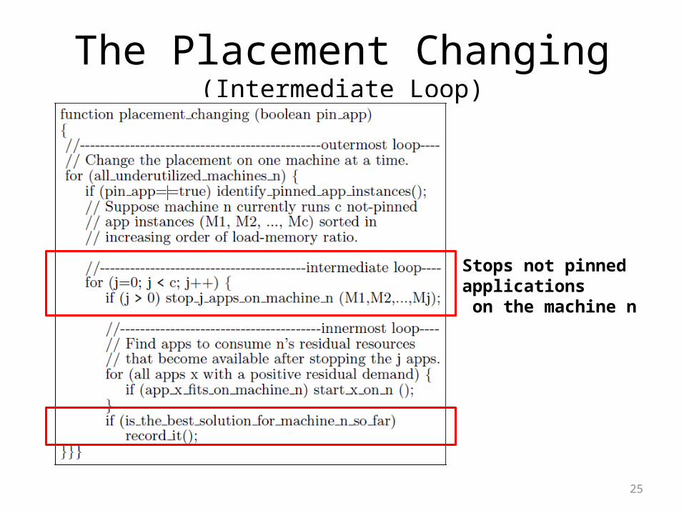
The Placement Changing (Intermediate Loop)

Stops not pinned applications on the machine n

26

The Intermediate Loop• Suppose machine n currently runs c not pinned application instances

– sorts the not-pinned application instances in increasing order of load-memory ratio (M1 , M2 ,….., Mc )

• In iteration j , it stops on machine n the j applications (M1,M2,..,Mc)– 0 ≤ j ≤ c

• Asks the innermost loop to find appropriate applications to consume machine n's residual resources that become available after stopping the j applications.– the number of stopped applications from 0 to c, it collects c + 1 placement

solutions, among which it picks as the final solution the one that leads to the highest CPU utilization of machine n

27

The Placement Changing (Innermost Loop)

Find apps with residual CPU demand and become available after stopping apps

28

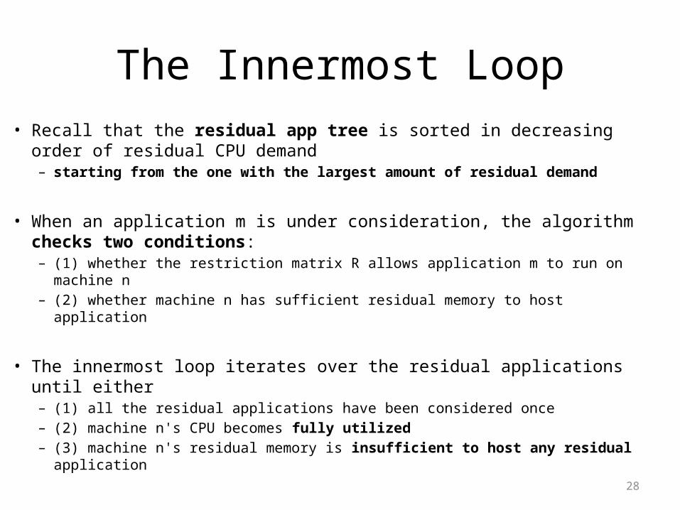
The Innermost Loop• Recall that the residual app tree is sorted in decreasing order of

residual CPU demand– starting from the one with the largest amount of residual demand

• When an application m is under consideration, the algorithm checks two conditions:– (1) whether the restriction matrix R allows application m to run on machine n– (2) whether machine n has sufficient residual memory to host application

• The innermost loop iterates over the residual applications until either– (1) all the residual applications have been considered once– (2) machine n's CPU becomes fully utilized– (3) machine n's residual memory is insufficient to host any residual application

29

The Full Placement Algorithm

Reuse the load-balancing component from an exiting algorithm [6]

[6]A. Karve, T. Kimbrel, G. Pacici, M. Spreitzer, M. Steinder, M. Sviridenko, and A. Tantawi. DynamicApplication Placement for Clustered WebApplications. In the International World Wide Web Conference (WWW), May 2006.

30

Pinned Instances

• Each application m has its own pinning threshold– Too low, may introduce many unnecessary placement changes– Too high, the total satisfied demand may be low

• The algorithm dynamically computes the pinning threshold for each application using information gathered in a dry-run – The dry run pins no application instances

31

Pinning Threshold

• Pinning the application instances whose load is higher than or equal to the pinning threshold

• how to compute the pinning threshold( )

– denote the minimum load assigned to a new instance of application m started in the dry run

– is the residual demand of application m after the dry run

32

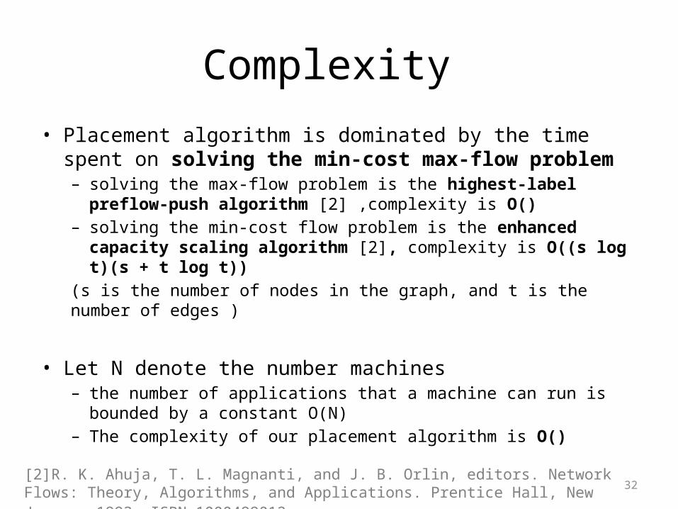
Complexity

• Placement algorithm is dominated by the time spent on solving the min-cost max-flow problem– solving the max-flow problem is the highest-label preflow-push

algorithm [2] ,complexity is O()– solving the min-cost flow problem is the enhanced capacity scaling

algorithm [2], complexity is O((s log t)(s + t log t))(s is the number of nodes in the graph, and t is the number of edges )

• Let N denote the number machines– the number of applications that a machine can run is bounded by a

constant O(N)– The complexity of our placement algorithm is O()

[2]R. K. Ahuja, T. L. Magnanti, and J. B. Orlin, editors. Network Flows: Theory, Algorithms, and Applications. Prentice Hall, New Jersey, 1993. ISBN 1000499012.

33

Practical Issues

• For the sake of brevity, our formulation of the placement problem and our algorithm description omit several practical issues– minimum/maximum number of instances– It’s possible that multiple instances of the same

application need to run on a single machine– actual start and stop of application instances should be

carefully

34

EXPERIMENTAL RESULTS• Compares it with the state-of-the-art algorithm [6]

proposed by Kimbrel et al • In the experiments– The configuration of machines is uniformly distributed over

the set {1GB:1GHz, 2GB:1.6GHz,3GB:2.4GHz, 4GB:3GHz}– The memory requirement of applications is uniformly

distributed over the set {0.4GB, 0.8GB, 1.2GB, 1.6GB}

[6]A. Karve, T. Kimbrel, G. Pacici, M. Spreitzer, M. Steinder, M. Sviridenko, and A. Tantawi. DynamicApplication Placement for Clustered WebApplications. In the International World Wide Web Conference (WWW), May 2006.

35

Problem Hardness(1/2)• CPU Load Factor

– It is defined as the ratio between the total CPU demand and the total CPU capacity

• Memory Load Factor – Let denote the average memory requirement of applications, and

denote the average memory capacity of machines

• Application Demand Distribution– Uniform distribution– Powerlaw distribution

36

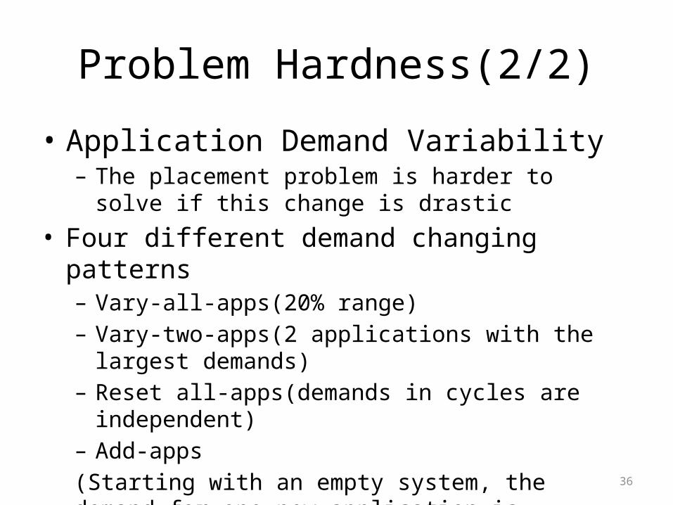
Problem Hardness(2/2)

• Application Demand Variability– The placement problem is harder to solve if this change is

drastic

• Four different demand changing patterns– Vary-all-apps(20% range)– Vary-two-apps(2 applications with the largest demands)– Reset all-apps(demands in cycles are independent)– Add-apps(Starting with an empty system, the demand for one new application is introduced into the system in every cycle)

37

Performance Results

38

Performance Results

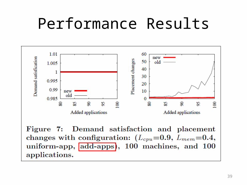
39

Performance Results

40

Performance Results

41

Performance Results

42

Conclusion

• Proposed an application placement controller – dynamically starts and stops application instances in

response to changes in application demands– allows multiple applications to share a single machine

• Under multiple resource constraints– maximize the total satisfied application demand– minimize the number of application starts and stops– to balance the load across machines

43

Comment

• It’s Useful for Plan B in NTU Cloud(Peak Load Service Quality Guaranteed Service)But – How to decide CPU & memory consumption– How to Guaranteed Service

• Environment is different– Physical Machine v.s. Virtual Machine