
Model Sailing Club Of the Chesapeake Sailing Bay Maritime ...
BSc Research Project
A SAILING SPEED ADVISORY FOR THE BEREZINA
Authors: R. van der Bles, J. Termorshuizen, S.M.A. Tjin-A-Djie, E.G. de Waal
1st Supervisor: M. Godjevac, PhD.2nd Supervisor: Prof.dr.ir. T.J.C. van Terswisga
Submitted to the Department of Maritime Engineering on December 19, 2014 inpartial fulfillment of the requirements for the degree of Bachelor of Science in
Maritime Engineering

Abstract
A ship sailing in shallow inland waters experiences shallow water effects. These effects causean increase in ship resistance, a decrease in sailing speed and an increase in fuel consumption.This report focuses on the shallow water effects that are experienced by the Berezina, an oldtug boat functioning as a platform to test maritime innovations and techniques in the fieldof sustainability. By adapting the sailing speed to the water depth the increase in resistanceis repulsed and therefore a reduction in fuel consumption is achieved. Various methods havebeen proposed to quantify the resistance increase by scientists such as Schlichting, Lackenby,Millward, Kamar and Jiang. All methods focus on wave resistance or viscous resistance andneither one of them combine these components. It is chosen to carry out a literature study intothe shallow water correction methods of abovementioned scientists and match these methodswith speed trials conducted on board the Berezina. The Holtrop & Mennen resistance predictionmethod is used as a baseline for the matching. The matching shows that the best fitting shallowwater correction method is that of Jiang. Based upon this method a scenario simulator wasprogrammed in which different scenarios were tested. Chapter 5 covers the literature study andchapter 6 discusses the procedure of conducting speed trials and the processing of the resultsobtained by them. Chapter 7 contains the matching of the correction methods found during theliterature study with the results obtained by the speed trials and Holtrop & Mennen. Chapter 8shows the design and working of the scenario simulator and the results that were obtained fromit. Conclusions emerging from the research project are given in chapter 9 and finally, in chapter10 recommendations for further research are included. Thanks go out to Milinko Godjevac andTom van Terwisga who supervised us during this research project. Also, we would like to thankErik Rotteveel for contributing a clear vision on the correction methods. Finally, we would liketo thank Robert Hekkenberg and Ido Akkerman for providing useful feedback on the study, theresearch and the report itself.

Nomenclature
Roman Variables
Am Midship area [m2]
AOD Lateral projected area of superstructures etc. on deck [m2]
Aw Waterline area [m2]
AXV Area of maximum transverse section exposed to the wind [m2]
AY V Projected lateral area above the water line [m2]
B Beam [m]
CAA Wind resistance coefficient
CALF Additional coefficient caused by three-dimensional flow effects
cb Block coefficient
CF Frictional resistance coefficient
CLF Additional coefficient caused by longitudinal flow
cm Midship coefficient
CMC Horizontal distance from midship section to centre of lateralprojected area AY V [m]
cp Prismatic coefficient
cwp Waterplane coefficient
CXLI Additional coefficient caused by the linear potential theory
D Depth [m]
1

2
Fnh Froude depth number
g Gravitational acceleration [9.81 m/s2]
h Water depth [m]
HBR Height of top of superstructure [m]
k Form factor
ke Number of engines
kp Number of propellers
L see LOA
LCB Longitudinal center of buoyancy [m]
LOA Length overall [m]
LPP Length between perpendiculars [m]
LWL Length of the water line [m]
MB Engine brake torque [Nm]
mf Mass flow of fuel [kg/s]
MP Propeller torque [Nm]
MS Shaft torque [Nm]
ne Engine speed [rev/s]
np Propeller speed [rev/s]
PB Brake power [W]
PE Effective towing power [W]
PO Open water propeller power [W]
PP Delivered propeller power [W]
PS Shaft power [W]
PT Thrust power [W]
Q Torque [Nm]
RA Resistance increase due to the correlation between model and ship [N]
RAA Resistance increase due to relative wind [N]

3
RAPP Resistance increase due to appendages [N]
RB Resistance increase due to bulbous bow [N]
RF Resistance increase due to friction [N]
RT Total ship resitance [N]
RTR Resistance increase due to stern [N]
Rw Resistance increase due to wave-making and wave-breaking [N]
Sbm Maximum bow squat [m]
sfc Specific fuel consumption [kg/Ws]
t Thrust deduction factor
T Draught [m]
Ta Draught at aft perpendicular [m]
Tf Draught at forward perpendicular [m]
V Sailing speed [m/s]
VE Effective sailing speed [m/s]
VS See V
VWR Relative wind speed [m/s]
V∞ Sailing speed in deep water [m/s]
w Wake factor
Weff Effective widt of the waterway [m]
zv Dynamic sinkage [m]

4
Greek Variables
α Half angle of entrance [◦]
ηGB Gearbox efficiency
ηH Hull efficency
ηO Open water propeller efficiency
ηR Relative rotative efficiency
ηS Shaft efficiency
ψWR Relative wind direction [◦]
θ Leading wave angle [◦]
ρ Density [kg/m3]

Contents
1 Introduction 12
2 Problem Definition 142.1 The Assignment and Main Challenges . . . . . . . . . . . . . . . . . . . . . . . . 142.2 The Berezina . . . . . . . . . . . . . . . . . . . . . . . . . . . . . . . . . . . . . . 152.3 Assignment Background . . . . . . . . . . . . . . . . . . . . . . . . . . . . . . . . 152.4 Main Goal, Main Question and Sub Questions . . . . . . . . . . . . . . . . . . . . 162.5 Hypothesis . . . . . . . . . . . . . . . . . . . . . . . . . . . . . . . . . . . . . . . 16
3 Objectives and Scope 173.1 Objectives . . . . . . . . . . . . . . . . . . . . . . . . . . . . . . . . . . . . . . . . 173.2 Scope . . . . . . . . . . . . . . . . . . . . . . . . . . . . . . . . . . . . . . . . . . 17
4 Work Plan 194.1 Literature . . . . . . . . . . . . . . . . . . . . . . . . . . . . . . . . . . . . . . . . 194.2 Speed Trials . . . . . . . . . . . . . . . . . . . . . . . . . . . . . . . . . . . . . . . 194.3 Scenario Simulation . . . . . . . . . . . . . . . . . . . . . . . . . . . . . . . . . . 20
5 Literature 225.1 Definition of Shallow Water . . . . . . . . . . . . . . . . . . . . . . . . . . . . . . 22
5.1.1 Division between Deep and Shallow Water . . . . . . . . . . . . . . . . . . 225.1.2 Distinction within Shallow Water . . . . . . . . . . . . . . . . . . . . . . . 23
5.2 Shallow Water Effects . . . . . . . . . . . . . . . . . . . . . . . . . . . . . . . . . 265.2.1 Viscous Flow and Form Factor . . . . . . . . . . . . . . . . . . . . . . . . 265.2.2 Wave Resistance . . . . . . . . . . . . . . . . . . . . . . . . . . . . . . . . 265.2.3 Sinkage and Trim . . . . . . . . . . . . . . . . . . . . . . . . . . . . . . . . 265.2.4 Hull Efficiency and Open Water Efficiency . . . . . . . . . . . . . . . . . . 265.2.5 Squat Effect . . . . . . . . . . . . . . . . . . . . . . . . . . . . . . . . . . . 27
5.3 Shallow Water Correction Methods . . . . . . . . . . . . . . . . . . . . . . . . . . 275.3.1 Schlichting (1934) . . . . . . . . . . . . . . . . . . . . . . . . . . . . . . . 275.3.2 Lackenby (1963) . . . . . . . . . . . . . . . . . . . . . . . . . . . . . . . . 285.3.3 Millward (1989) . . . . . . . . . . . . . . . . . . . . . . . . . . . . . . . . 285.3.4 Kamar (1996) . . . . . . . . . . . . . . . . . . . . . . . . . . . . . . . . . . 295.3.5 Jiang (2001) . . . . . . . . . . . . . . . . . . . . . . . . . . . . . . . . . . 29
5

CONTENTS 6
6 Speed Trial Tests 306.1 Procedure of Conducting Speed Trials . . . . . . . . . . . . . . . . . . . . . . . . 306.2 Processing of the Speed Trial Results . . . . . . . . . . . . . . . . . . . . . . . . . 31
6.2.1 Background Information . . . . . . . . . . . . . . . . . . . . . . . . . . . . 316.2.2 Speed Trial Results . . . . . . . . . . . . . . . . . . . . . . . . . . . . . . . 32
7 Matching of Literature and Speed Trial Tests 397.1 Theoretical Deep Water Resistance . . . . . . . . . . . . . . . . . . . . . . . . . . 39
7.1.1 Holtrop & Mennen Method . . . . . . . . . . . . . . . . . . . . . . . . . . 407.1.2 Van Oortmerssen Method . . . . . . . . . . . . . . . . . . . . . . . . . . . 407.1.3 Resistance Prediction . . . . . . . . . . . . . . . . . . . . . . . . . . . . . 417.1.4 The Berezina’s Resistance . . . . . . . . . . . . . . . . . . . . . . . . . . . 44
7.2 Power Estimation . . . . . . . . . . . . . . . . . . . . . . . . . . . . . . . . . . . . 457.3 Correction of the Speed Trial Results . . . . . . . . . . . . . . . . . . . . . . . . . 477.4 Speed Trial Results Compared to Holtrop & Mennen Results . . . . . . . . . . . 487.5 Applying Shallow Water Correction Methods . . . . . . . . . . . . . . . . . . . . 50
7.5.1 Schlichting (1934) . . . . . . . . . . . . . . . . . . . . . . . . . . . . . . . 517.5.2 Lackenby (1963) . . . . . . . . . . . . . . . . . . . . . . . . . . . . . . . . 527.5.3 Millward (1989) . . . . . . . . . . . . . . . . . . . . . . . . . . . . . . . . 537.5.4 Kamar (1996) . . . . . . . . . . . . . . . . . . . . . . . . . . . . . . . . . . 557.5.5 Jiang (2001) . . . . . . . . . . . . . . . . . . . . . . . . . . . . . . . . . . 57
7.6 Results . . . . . . . . . . . . . . . . . . . . . . . . . . . . . . . . . . . . . . . . . . 60
8 Scenario Simulation 618.1 Simulator . . . . . . . . . . . . . . . . . . . . . . . . . . . . . . . . . . . . . . . . 61
8.1.1 Simplifications . . . . . . . . . . . . . . . . . . . . . . . . . . . . . . . . . 618.1.2 Inner Workings of the Scenario Simulator . . . . . . . . . . . . . . . . . . 628.1.3 Speed Advisory . . . . . . . . . . . . . . . . . . . . . . . . . . . . . . . . . 648.1.4 Expectations . . . . . . . . . . . . . . . . . . . . . . . . . . . . . . . . . . 65
8.2 Results of the Scenario Simulation . . . . . . . . . . . . . . . . . . . . . . . . . . 658.2.1 Route 1 . . . . . . . . . . . . . . . . . . . . . . . . . . . . . . . . . . . . . 658.2.2 Route 2 . . . . . . . . . . . . . . . . . . . . . . . . . . . . . . . . . . . . . 668.2.3 Route 3 . . . . . . . . . . . . . . . . . . . . . . . . . . . . . . . . . . . . . 688.2.4 Route 4 . . . . . . . . . . . . . . . . . . . . . . . . . . . . . . . . . . . . . 69
9 Conclusions 70
10 Recommendations 7210.1 Validating the Speed Trial Results . . . . . . . . . . . . . . . . . . . . . . . . . . 7210.2 Shallow Water Correction Methods . . . . . . . . . . . . . . . . . . . . . . . . . . 7310.3 Validating the Scenario Simulator . . . . . . . . . . . . . . . . . . . . . . . . . . . 7310.4 Speed Optimization Algorithm . . . . . . . . . . . . . . . . . . . . . . . . . . . . 73
A Berezina Engine Specifications 76
B Main Specifications, Form Coefficients and Stern 77B.1 Main Specifications . . . . . . . . . . . . . . . . . . . . . . . . . . . . . . . . . . . 77B.2 Form Coefficients . . . . . . . . . . . . . . . . . . . . . . . . . . . . . . . . . . . . 79B.3 Stern . . . . . . . . . . . . . . . . . . . . . . . . . . . . . . . . . . . . . . . . . . . 80

CONTENTS 7
C Numerical Results of the Resistance Methods 81
D PropCalc 83D.1 Fixed Parameters . . . . . . . . . . . . . . . . . . . . . . . . . . . . . . . . . . . . 83D.2 Method . . . . . . . . . . . . . . . . . . . . . . . . . . . . . . . . . . . . . . . . . 83D.3 Input . . . . . . . . . . . . . . . . . . . . . . . . . . . . . . . . . . . . . . . . . . . 84D.4 Matching . . . . . . . . . . . . . . . . . . . . . . . . . . . . . . . . . . . . . . . . 84
E Output of the Power Estimation 87
F MatLab Code of the Simulator 89

List of Figures
5.1 Leading wave decay (n) as a function of depth-length ratio (h/L). [21] . . . . . . 255.2 Bow wave angle as a function of Froude depth number. [21] . . . . . . . . . . . . 25
6.1 Map of the Mooie Nel and Noorder Buiten Spaarne, near Haarlem. . . . . . . . . 316.2 Relative wind of runs 1 and 2. . . . . . . . . . . . . . . . . . . . . . . . . . . . . . 366.3 Relative wind of runs 3 and 4. . . . . . . . . . . . . . . . . . . . . . . . . . . . . . 366.4 Relative wind of runs 5 and 6. . . . . . . . . . . . . . . . . . . . . . . . . . . . . . 376.5 Relative wind of runs 7 and 8. . . . . . . . . . . . . . . . . . . . . . . . . . . . . . 376.6 Relative wind of runs 9 and 10. . . . . . . . . . . . . . . . . . . . . . . . . . . . . 386.7 Relative wind of runs 11 and 12. . . . . . . . . . . . . . . . . . . . . . . . . . . . 38
7.1 Input for the Holtrop & Mennen resistance method. . . . . . . . . . . . . . . . . 427.2 Results from the Holtrop & Mennen resistance method. . . . . . . . . . . . . . . 427.3 Input for the Van Oortmerssen resistance method. . . . . . . . . . . . . . . . . . 437.4 Results from the Van Oortmerssen resistance method. . . . . . . . . . . . . . . . 437.5 Results from the Holtrop & Mennen- and the Van Oortmerssen resistance methods. 447.6 Corrected power and resistance for the Berezina’s speed trial results. . . . . . . . 487.7 Speed trials and Holtrop & Mennen resistance values. . . . . . . . . . . . . . . . 487.8 Speed trial resistances compared with Holtrop & Mennen resistance curves, cor-
rected for different values of CF . . . . . . . . . . . . . . . . . . . . . . . . . . . . 507.9 Different channel types, according to Briggs. [1] . . . . . . . . . . . . . . . . . . . 577.10 Berezina’s resistance-speed curves at h = 2.3m. . . . . . . . . . . . . . . . . . . . 60
8.1 The Graphical User Interface of the simulator. . . . . . . . . . . . . . . . . . . . 638.2 The Graphical User Interface of the simulator after running calculations. . . . . . 648.3 Route 1: Constant depth profile. . . . . . . . . . . . . . . . . . . . . . . . . . . . 658.4 Route 2: A single depth change of 2m. . . . . . . . . . . . . . . . . . . . . . . . . 668.5 Route 2: Fuel savings at different mean Froude depth numbers. . . . . . . . . . . 678.6 Route 2: At mean Froude depth number 0.7017. . . . . . . . . . . . . . . . . . . 678.7 Route 3: Varying water depth profile. . . . . . . . . . . . . . . . . . . . . . . . . 688.8 Route 3: Fuel savings at different mean Froude depth numbers. . . . . . . . . . . 688.9 Route 4: A single depth change of 10m. . . . . . . . . . . . . . . . . . . . . . . . 69
A.1 Torque curve of the VW TDI 120-5. [26] . . . . . . . . . . . . . . . . . . . . . . . 76
B.1 Main dimensions of a vessel. . . . . . . . . . . . . . . . . . . . . . . . . . . . . . . 77B.2 Definition of the half angle of entrance. . . . . . . . . . . . . . . . . . . . . . . . 78B.3 Standard shapes for cross sectional areas. . . . . . . . . . . . . . . . . . . . . . . 80
8

LIST OF FIGURES 9
C.1 Numerical overview of the results of the Holtrop & Mennen method. . . . . . . . 81C.2 Numerical overview of the results of the Van Oortmerssen method. . . . . . . . . 82
D.1 Optimization methods PropCalc. . . . . . . . . . . . . . . . . . . . . . . . . . . . 84D.2 Input for PropCalc. . . . . . . . . . . . . . . . . . . . . . . . . . . . . . . . . . . . 84D.3 Open water diagram for propeller B3-65. . . . . . . . . . . . . . . . . . . . . . . . 86
E.1 Output of the power estimation. . . . . . . . . . . . . . . . . . . . . . . . . . . . 88

List of Tables
2.1 Main dimensions of the Berezina. . . . . . . . . . . . . . . . . . . . . . . . . . . . 15
4.1 Work plan for the research project, per category. . . . . . . . . . . . . . . . . . . 204.2 Work plan for the research project, per document. . . . . . . . . . . . . . . . . . 21
5.1 Shallow water characterization summary. [20] . . . . . . . . . . . . . . . . . . . . 23
6.1 Power and torque according to Volkswagen Marine. [26] . . . . . . . . . . . . . . 326.2 Average values of the measured parameters during speed trials. . . . . . . . . . . 336.3 Non-dimensional parameters for components of the wind resistance coefficient. [3] 346.4 Calculated components of CAA. . . . . . . . . . . . . . . . . . . . . . . . . . . . . 346.5 Calculation of CAA and RAA. . . . . . . . . . . . . . . . . . . . . . . . . . . . . . 35
7.1 Limitations to the Holtrop & Mennen method and variety in vessel types. [17] . 407.2 Limitations to the Van Oortmerssen method compared with the Berezina’s pa-
rameters. [25] . . . . . . . . . . . . . . . . . . . . . . . . . . . . . . . . . . . . . . 407.3 Main specifications of the Berezina. . . . . . . . . . . . . . . . . . . . . . . . . . . 417.4 Efficiencies and constant assumed for the Berezina’s engine. . . . . . . . . . . . . 477.5 Numerical values and ratio of the Van Ootmerssen and the Holtrop & Mennen
method. . . . . . . . . . . . . . . . . . . . . . . . . . . . . . . . . . . . . . . . . . 497.6 Results after correction by Schlichting’s method. . . . . . . . . . . . . . . . . . . 517.7 Results after correction by Lackenby’s method. . . . . . . . . . . . . . . . . . . . 527.8 Results after correction by Millward’s method. . . . . . . . . . . . . . . . . . . . 537.9 Results after correction by Millward’s method. (2) . . . . . . . . . . . . . . . . . 547.10 Results after correction by Kamar’s method. . . . . . . . . . . . . . . . . . . . . 557.11 Results after correction by Kamar’s method. (2) . . . . . . . . . . . . . . . . . . 567.12 Water depth draught coefficients. . . . . . . . . . . . . . . . . . . . . . . . . . . 577.14 Various methods and their applicability to calculate the dynamic sinkage. [1] . . 587.13 Length - water depth coefficients. . . . . . . . . . . . . . . . . . . . . . . . . . . . 587.15 Results for the maximum bow squat calculation, using Millward’s equation. . . . 597.16 Results after correction by Jiang’s method. . . . . . . . . . . . . . . . . . . . . . 597.17 Results after correction by Jiang’s method. (2) . . . . . . . . . . . . . . . . . . . 60
A.1 Specifications of the VW TDI 120-5. [26] . . . . . . . . . . . . . . . . . . . . . . 76
D.1 Fixed parameters of the current propeller design. . . . . . . . . . . . . . . . . . . 83D.2 Range of possible propeller designs. . . . . . . . . . . . . . . . . . . . . . . . . . . 85D.3 Diameter and P/D ratios for various propellers. . . . . . . . . . . . . . . . . . . . 85
10

LIST OF TABLES 11
D.4 Estimated design parameters for propeller B3-65. . . . . . . . . . . . . . . . . . . 86

Chapter 1
Introduction
A reduction in fuel consumption of 10% could be achieved when adjusting the Berezina’s sailingspeed to the water depth on inland waterways. This statement is the hypothesis of this report,which is specified for the Berezina. The Berezina is an old tug boat, which is nowadays usedas an ‘Energy ship’ for the Fair Nature foundation. The vessel functions as a platform to testmaritime innovations in the field of sustainability.
It has been proven that sailing in shallow or confined waters has a negative influence on theperformance of a vessel. As can be noticed in practice and has been shown in earlier researchprojects, the resistance of a vessel increases when it sails in shallow or confined waters. Therefore,a correlation between the increase in resistance and the change in water depth has to be found.If there is such a correlation it could be used to adjust the sailing speed in order to decrease theresistance at a constant water depth.
So far, a number of researches have been performed to determine the effects of sailing in shallowwater on the resistance of a vessel. This research project is based on the papers written bySchlichting (1934), Lackenby (1963), Millward (1989), Kamar (1996) and Jiang (2001), who alldeveloped correction methods to compensate for the added resistance effects of sailing in shallowwaters. The methods of Schlichting and Lackenby focus on the added wave resistance due tosailing in shallow waters, where Millward and Kamar correct for the effects on the viscous resis-tance. The focus of Jiang’s research is on the influence of the dynamic sinkage on the resistanceof a vessel.
The main goal of this research project is to reduce the Berezina’s fuel consumption over apredefined route, compared to the fuel consumption of the Berezina when sailing the same routeat a constant speed. This goal has to be accomplished by adapting the sailing speed to the waterdepth. In order to adjust the sailing speed in such a way that fuel reduction can be achievedan educated advisory speed must be given. Therefore an applicable correction method for theshallow water effects, experienced by the Berezina, has to be found. Research should turn out ifone of the existing methods could be used or a new correction method has to be developed. Even-tually, the correction method is implemented into a scenario simulation model, which simulatesroutes with routes with various depth profiles.
12

CHAPTER 1. INTRODUCTION 13
The report consists of three parts. The first part consists of a literature study on the definitionof shallow water and the effects of shallow water on the resistance of a vessel. The second partincludes a determination of the resistance obtained by the speed trial measurements. The speedtrial results are to be validated by the results of the Holtrop & Mennen resistance predictionmethod. The influence of each correction method on the total resistance is calculated for andcompared to the shallow water condition. Finally a suitable correction method is chosen. In thethird part various simulations are performed to give an indication of the amount of fuel whichcan be saved by adapting the sailing speed to the changing water depth. The results of thescenario simulation are based on the chosen correction method.
Following this study, the results of adjusting the sailing speed in relation to the changing waterdepth on the amount of consumed fuel will be clarified.

Chapter 2
Problem Definition
In this chapter the main goal and the background of the assignment are clarified. The assignmentcan be found in section 2.1. Section 2.2 covers details of the Berezina, the tugboat that is usedas the reference ship for this research project. In section 2.3 the background of the assignmentfor the project is explained. The main goal and the raised main- and sub questions are specifiedin section 2.4. This chapter ends with a hypothesis, given in section 2.5.
2.1 The Assignment and Main Challenges
As can be noticed in practice and has been shown in earlier research projects, the resistance ofa ship increases when it sails in shallow or confined waters. An increase in resistance will leadto higher fuel consumption. Therefore, the assigment is to find a correlation between a vessel’sresistance increase and the water depth. This research project will focus on defining a vessel’sresistance as a function of the speed with respect to the water depth. The goal is to providea sailing speed advisory in which the speed is adapted to the water depth which will lead to adecrease in resistance and therefore a decrease in fuel consumption. The reference ship is theBerezina, more information on the Berezina can be found in the next section. The sailing speedadvisory will be customized for the Berezina.
The main challenges in this assignment are:
1. finding a correlation between water depth and speed;This correlation can be found when a correlation between the water depth and resistanceincrease and a correlation between the resistance increase and the sailing speed is found.It is important to find such a correlation because it will give an indication on how muchinfluence the water depth has on the resistance land sailing speed of the vessel and thus onthe toal fuel consumption of the vessel on a given route with set time limit.
2. determining the accuracy of the speed trial measurements;The speed trial results will form a reference for the programming of the sailing speed advi-sory. The results need to be as accurate as possible to provide a realistic reference.
3. validating the sailing speed advisory.The sailing speed advisory can be validated by means of test runs with the Berezina to seeif the output provided by the advisory are corresponding to the real-time output.
14

CHAPTER 2. PROBLEM DEFINITION 15
The societal problem that is to be solved is the exhaust of polluting gasses into the air due toinland shipping. The underlying thought of this research is to eventually reduce this amount ofexhaust gasses. A reduction of the fuel consumption on a predefined route leads to a reduction ofharmful exhaust gasses as fuels content harmful components. This reduction in fuel consumptionis to be achieved by reducing the resistance increase of the ship due to shallow water effects.
2.2 The Berezina
The Berezina will be the reference ship for this research project. The Berezina is an old tugboatthat is nowadays used as an “Energy Ship” for the Fair Nature Foundation 1, a foundation thatfocuses on issues like climate change, consumer behavior and sustainable energies. The founda-tion is engaged in the enlightenment of people on these subjects and it stimulates people to startprojects that deal with energy problems. The Berezina functions as a platform to test maritimeinnovations and techniques in the field of sustainability. The dimensions of the Berezina aregiven in table 2.1. Specifications of the engine of the Berezina can be found in Appendix A.
LOA [m] 20.6LPP [m] 18.6B [m] 4.59T [m] 1.30D [m] 2.14
Table 2.1: Main dimensions of the Berezina.
2.3 Assignment Background
The assignment is a response to the work produced by M. Godjevac and K.H. van der Meij [4] forthe EU project MoveIT wherein measurements have been done on the performance of Europeaninland ships. It was concluded that the variation in operational conditions is mainly causedby fluctuation of water level. The main focus in this research is therefore the effect of shallowwater on ships, with respect to the water depth. Because the Berezina is the reference ship allconclusions will be drawn with regard to this ship.
A number of papers have been written about the effects of shallow water on the resistance ofvessels. During this research project, the theories and correction methods of Schlichting (1934)[23], Lackenby (1963) [13], Millward (1989) [16], Kamar (1996) [10] and Jiang (2001) [9] aretaken into consideration. An oversight of these different theories and publications can be foundin section 5.3.
There are several methods to determine the effect of shallow water on the speed of a vessel,however none of these methods deal with all aspects of the effect of shallow water. That is notto say that the methods are unuseful, but there is no correction method that is generally statedto be correct for all ships. The objective of this research project is to find a correction methodthat is applicable to the Berezina by matching the abovementioned methods and the speed trialresults. This should result in a reduction in fuel consumption. The objectives and scope arefurthermore explained in chapter 3.
1http://www.fairnature.org/

CHAPTER 2. PROBLEM DEFINITION 16
2.4 Main Goal, Main Question and Sub Questions
The main goal of this research project is to achieve a reduction in fuel consumption for theBerezina. This reduction should be accomplished by adapting the sailing speed to the waterdepth. By adapting the sailing speed to the water depth, the resistance will decrease and thefuel consumption will be reduced. One of the goals is creating a scenario simulator which pro-vides a sailing speed advice to the ship owner of the Berezina while not compromising on theintended arrival time. More information about the design of the scenario simulator can be foundin section 3.2.
To achieve satisfying results, real time measurements have to be done to acquire the ship’sresistance curves by means of on-board speed trial tests. The research project is successful whena mathematical model is produced which gives reliable results and can be used to reduce the fuelconsumption of the Berezina.
Good research always starts with the construction of a main question and sub questions. Theresistance of a vessel sailing in shallow and confined waterways, with respect to the water depthis the unknown parameter in this research. Adapting the sailing speed to varying water depthand resistance should lead to a reduction of the fuel consumption. To investigate the interactionbetween the water depth and the sailing speed, the following main research question is raised:
To which extent can the fuel consumption of the Berezina be reduced, when the vessel’ssailing speed is varied in shallow waters on inland waterways, with respect to the waterdepth?
To achieve an answer to this main question the following sub questions have been raised:
1. When is water shallow?
2. How does the water depth influence the resistance of the vessel?
3. How can a correction, due to the variation in water depth, in the vessels resistance becalculated?
4. What is the influence of the change in water depth on the fuel consumption?
5. How can all these relations be combined to achieve reduction of fuel consumption?
Answering these questions one by one should provide enough information to construct a scenariosimulator by which different scenarios of a ship sailing in shallow and confined waters can besimulated. Adapting the sailing speed to the varying water depth should lead to a reduction infuel consumption and an answer to the main question will be given by means of the scenariosimulation.
2.5 Hypothesis
The main goal of this research is to reduce the Berezina’s fuel consumption by adjusting thesailing speed in relation to the water depth when sailing in shallow waters. To give an indicationof the expected results, the hypothesis has been raised:
If the sailing speed is adjusted to the effects of sailing in shallow water, then a 10 % reduc-tion of fuel consumption will be achieved.

Chapter 3
Objectives and Scope
In this chapter the objectives and the scope of the research project are stated. Section 3.1contains the objectives of the research project. This section provides the goals which are to beachieved with this project. Section 3.2 provides the parameters to which the research projectwill be confined in its entirety.
3.1 Objectives
The research project contains four objectives. These are as follows:
1. Learning about the possible effects of sailing in shallow waers on the resistance of a vessel.
2. Obtaining the resistance of the Berezina by means of speed trial tests on board the Berezinafollowing the procedures and guidelines provided by the ITTC [7].
3. Comparing existing shallow water effect correction methods with results of the speed trialtests and match the methods and the speed trial test results so that the programming of ascenario simulator can be constructed.
4. Creating a scenario simulator which provides an advice on the sailing speed when adaptedto the water depth in shallow water so that a reduction in fuel consumption will be achieved.
3.2 Scope
The research project is subjected to a set of parameters that confine it so that it is possible todo this project within the given time. The boundaries are drawn up as follows:
1. The research is done solely on the Berezina. The mathematical model will be specified forthe properties of the Berezina.
2. The width of the waterway is not taken into account, neither are the consequential effects.
3. The effects of current and waves are considered non-existent because they are expected tobe negligible in the waterway during the conduction of on-board speed trial tests.
4. A scenario simulator will be used because the programming involved to use actual maps ofwaterways is too complex to do in the time given for the research project.
17

CHAPTER 3. OBJECTIVES AND SCOPE 18
The scenario simulator mentioned in the fourth boundary as listed above is also subjected to aset of boundaries. The boundaries concerning the scenario simulator are as follows:
1. It is assumed that the vessel’s heading is constant, the ship sails straight forward and noturns are to be taken.
2. The arrival time for the Berezina’s destination is fixed and therefore the arrival time is notto be changed when the sailing speed is adapted.
3. The water depth does not vary gradually. Instead, the water depth varies instantaneously.
4. In the scenario simulator the effects of wind are not taken into account for the speed trialswill already be corrected for the influence of the wind.
5. It is assumed that the vessel’s sailing speed is varied instantaneously.
6. The Berezina has a speed limit of 9,2 knots.
Section 8.1.1 contains more boundaries and simplifications regarding the scenario simulation.

Chapter 4
Work Plan
In this chapter the overall project approach is clarified. The different aspects of the researchproject are divided up into three categories: a literature study, speed trials and a scenariosimulation. The approach of the first aspect which is the literature study can be found in section4.1. The second aspect is the experimental part of the research: the conduction of speed trialson board the Berezina. Section 4.2 contains an explanation and a justification of these speedtrials. The third and last section, section 4.3 encloses the final part of the project which is ascenario simulation. Table 4.1 and table 4.2 contain extensive plans of all the tasks that need tobe done, including the distribution of the tasks between the group members concerning chapters1 to 9 and a time planning for the chapters 5 to 9 that contain information leading to a satisfyinganswer to the main question and sub questions.
4.1 Literature
After collecting literature, five theories have been selected which will be further elaborated onin section 5.3. These theories were published by Schlichting [23], Lackenby [13], Millward [16],Kamar [10] and Jiang [9]. The collected literature is used to find a definition of the sailing speedcorrection appropriate for the Berezina when experiencing shallow water effects. The results ofthe literature study are compared and matched to the results of the speed trials to verify that thedefined corrections are valid for and in accordance with the effects that the Berezina experiences.The matching process can be found in chapter 7.
4.2 Speed Trials
In order to apply sailing speed corrections to the Berezina, the ship’s resistance needs to bedefined for it is the resistance of the vessel that is affected by shallow water effects. An estimationof the ship’s resistance can be achieved by conducting speed trials. For conducting on board speedtrials the vessel’s dimensions and the specifications of the vessel’s engine have to be known.The speed trials are conducted according to the guidelines of the International Towing TankConference, or shortly ITTC [7]. Parameters that are variable and determined during the speedtrials are water depth, sailing speed and heading of the ship, but also wind direction and windspeed. An extended overview of the conduction of speed trials and the results of the speed trialscan be found in chapter 6.
19

CHAPTER 4. WORK PLAN 20
4.3 Scenario Simulation
A satisfying answer to the main question “To which extent can the fuel consumption of the Berez-ina be reduced, when the vessel’s sailing speed is varied in shallow waters on inland waterways,with respect to the water depth?” can be achieved by comparing the fuel consumption in thesituation without adapting the sailing speed, to the fuel consumption of the vessel when on thesame route, within the same length of time, the sailing speed is adapted with respect to the waterdepth. Due to limited duration of the research project, the decision has been made to create anumber of 4 datasets which represent possible routes on which the Berezina sails, with varyingwater depth and varying lenght. These possible routes represent different scenarios that couldbe faced by the Berezina and will be tested and compared by means of scenario simulation. Theboundaries that are set for the scenario simulation can be found in section 3.2. A further elabo-ration of the simulator can be found in chapter 8 in which also the outcomes of the simulationand a clarification of the outcome of the different scenarios can be found.
Task Responsible Person(s) DeadlineLiterature studyCollect Literature All September 22, 2014Determine what Information is Useful All September 24, 2014Document Correction Methods Roel van der Bles, December 5, 2014
Lisa de WaalDocument Power Estimation Jelmar Termorshuizen December 12, 2014Document Matching of Methods and Speed Trials Stephanie Tjin-A-Djie December 12, 2014Speed TrialsPrepare Speed Trials Stephanie Tjin-A-Djie October 14, 2014Conduct Speed Trials All October 14, 2014Document Speed Trials - Procedures Stephanie Tjin-A-Djie December 12, 2014Document Speed Trials - Results Stephanie Tjin-A-Djie December 12, 2014Scenario SimulationDesign Simulator Roel van der Bles December 3, 2014
Document Goal of the Simulation Jelmar Termorshuizen December 15, 2014Create Various Scenarios Roel van der Bles December 12, 2014Run Scenarios and Draw Conclusions Roel van der bles, December 15, 2014
Jelmar Termorshuizen
Table 4.1: Work plan for the research project, per category.

CHAPTER 4. WORK PLAN 21
Document Responsible Person(s) DeadlinePlan of ApproachDocument Summary Jelmar Termorshuizen September 25, 2014Document Introduction Roel van der Bles September 25, 2014Document Problem Definition Jelmar Termorshuizen September 23, 2014Document Literature Lisa de Waal September 23, 2014Document Overall Project Approach Lisa de Waal September 23, 2014Document Plan of Approach Primary Research Stephanie Tjin-A-Djie September 23, 2014Document Conclusions Roel van der Bles September 25, 2014Compose and Finalize Plan of Approach Lisa de Waal October 1, 2014Final ReportDocument Abstract Lisa de Waal December 16, 2014Document Introduction Jelmar Termorshuizen December 16, 2014Document Problem Definition Stephanie Tjin-A-Djie, November 28, 2014
Lisa de WaalDocument Objectives & Scope Stephanie Tjin-A-Djie November 28, 2014
Lisa de WaalDocument Work Plan Lisa de Waal November 2014Document Literature Study Roel van der Bles, December 5, 2014
Lisa de WaalDocument Speed Trials Stephanie Tjin-A-Djie December 5, 2014Document Matching Literature & Speed Trials Jelmar Termorshuizen, December 14, 2014
Stephanie Tjin-A-DjieDocument Scenario Simulation Roel van der Bles, December 15, 2014
Jelmar TermorshuizenDocument Conclusions Stephanie Tjin-A-Djie December 16, 2014Document Recommendations Roel van der Bles December 16, 2014Compose and Finalize Final Report Lisa de Waal December 16, 2014PaperCompose Paper Stephanie Tjin-A-Djie December 12, 2014Finalize Paper Lisa de Waal December 17, 2014
Table 4.2: Work plan for the research project, per document.

Chapter 5
Literature
This chapter covers the literature study part of the research project. The first section, section5.1 contains a definition of the division between deep and shallow water. The first sub question,When is water shallow?, is answered after this section. In section 5.2 the different effects vesselsexperience when sailing in shallow water are given. The correction methods mentioned in sec-tion4.1, the theories defined by Schlichting [23], Lackenby [13], Millward [16], Kamar [10] andJiang [9] are explained and worked out in section 5.3 .
5.1 Definition of Shallow Water
In order to investigate the impact of shallow water on the resistance and therefore the sailingspeed, a definition of shallow water is required. This section provides such a division betweendeep water and shallow water in the first subsection: subsection 5.1.1. Subsection 5.1.2 containsa further distinction within the domain of shallow water.
5.1.1 Division between Deep and Shallow Water
A clear-cut definition of when a vessel is sailing in shallow water and thus experiencing shallowwater effects does not exist, for this complex problem is caused by multiple physical variables.Yet, a group of researchers at the Australian Maritime College of the University of Tasmania [20]has introduced guidelines for establishing whether ships are sailing in deep water or in shallowwater. The researchers have stated that water is deep if the Froude depth number is below 0.5.The Froude depth number can be found with equation 5.1 :
Fnh =V√gh
(5.1)
This definition implies that a vessel is sailing in shallow water whenever the Froude depth numberis higher than 0.5. A Froude depth number below 0.5 implicates that the ship is sailing in deepwater. This definition will be persevered during the research project.
22

CHAPTER 5. LITERATURE 23
5.1.2 Distinction within Shallow Water
Next to the difference between deep and shallow water a distinction can be made within the do-main of shallow water. Shallow water then can be labeled sub-critical, critical and super-critical.The distinction between deep water and shallow water and a summary of the categories withinthe domain of shallow water can be found in table 5.1. The researchers in Australia stated bydefinition that if one of the conditions belonging to the deep water operational zone is not met,the operational zone can be considered shallow water.
The distinction between sub-critical, critical en super-critical shallow water also depends onthe Froude depth number but the categorization is mostly based on wash characterizations: thewaves caused by a moving vessel. Table 5.1 shows that the wave system is divergent for any waterdepth. Those waves are observed as the wake of the vessel. Transverse waves are perpendicularto the direction of wave propagation. As the water depth decreases for a given speed, whichleads to an increase in Froude depth number, the divergent wave system increases to about 90◦.The transverse waves completely vanish in this situation and only the divergent wave systemremains.
Operational zoneCharacterization Deep Water Shallow Water Shallow Water Shallow Water
Sub-critical Critical Super-critical
Froude Depth Number Fnh < 0.5 0.5 < Fnh < 1.0 Fnh ' 1.0 Fnh > 1.0Divergent Wave System Yes Yes Yes Yes
Transverse Wave System Yes Diminishing None None
Leading Wave Angle Constant at 19◦28′ 19◦28′ 6 θ 6 90◦ θ ' 90◦ 90◦ 6 θLeading Wave Decay Constant at − 1
3 Variable f (Fnh) Variable f (Fnh) Variable f (Fnh)Wave System Dispersive Yes Diminishing No Increasing
Solitons No No Yes No
Spectral Wavelet Analysis Constant Variable with time Variable for fixed Fn Variable with time
Variable with time
Performance Constant with time Increasing Variable with time Reducing
(oscillating)
Table 5.1: Shallow water characterization summary. [20]
The next characterization is the angle of the leading wave. The change in leading wave angle goesalong with the change in transverse wave system. Figure 5.2 shows the outcome of the authors’previous research inter alia regarding divergent wave angle and decay [21]. The leading wave an-gle is called the bow wave angle in this case. An extrema in leading wave angle occurs at aroundFnh = 0.9. During the same research the leading wave decay coefficient was investigated. Asfigure 5.1 shows, the decay coefficient n turns out to be depending on the Froude depth numberand varies between -1.0 to -0.2 and is constant only in deep water, where Fnh < 0.5.
As shown in table 5.1, the only non-dispersive wave system is found in critical shallow wa-ter. This is where solitons appear. The researchers at the Australian Maritime College give thefollowing definition:
“A soliton is a single non-dispersive wave with no preceding or following trough.Solitons are cyclical and time dependent in nature.” [20]
Consequently, the only domain possibly showing solitons is that of critical shallow water.

CHAPTER 5. LITERATURE 24
The penultimate characterization is the spectral wavelet analysis. This is similar to Fourieranalysis as both techniques break down signals within a time domain into individual compo-nents. The next step is to plot the components in the frequency domain. The only difference isthat in wavelet analysis it is also possible to determine at which instant an event occurred withinthe signal. The wavelet analyses are to be reviewed with regard to the value, location and fre-quency of the peak spectral energy and the form and frequency range of the global spectral energy.
Finally, table 5.1 mentions performance as one of the characterizations. This performance isnot a wash characterization as such but also contributes to the distinction between the opera-tional zones. The performance depends among others upon resistance, sinkage and trim. Theresistance of a vessel changes as the water depth varies. The most noticeable change will be foundin sailing speed. Section 5.2 takes a closer look on this aspect. A different aspect is the sinkage.A vessel can be regarded as a free-floating body. It will sink and trim as the body is subjectedto forces. The constrained flow around the body causes a change in pressure which leads to asuction effect towards the boundary. A similar effect occurs when a vessel moves towards a bankor to other vessels. The vessel sinks and trims, and the phenomenon called squat will occur. Afurther elaboration on sinkage, trim and squat can be found in subsections 5.2.3 and 5.2.5. Themagnitude of squat depends directly upon the sailing speed, the hull form and the ratio betweenwater depth and ship draught.
The corrections found in the collected literature only consider the division between deep wa-ter and shallow water. Therefore the different operational zones within the domain of shallowwater will not be addressed.

CHAPTER 5. LITERATURE 25
Figure 5.1: Leading wave decay (n) as a function of depth-length ratio (h/L). [21]
Figure 5.2: Bow wave angle as a function of Froude depth number. [21]

CHAPTER 5. LITERATURE 26
5.2 Shallow Water Effects
The next step is to determine the effects shallow waters have on vessels. Sailing in shallowwater affects the resistance of the vessel, which can be divided into wave resistance and viscousresistance. It also has an effect on the trim and sinkage of the vessel and on the propulsiveefficiency of the vessel. In subsection 5.2.1 the effect on viscous flow and form factor are given.In subsection 5.2.2 the effects on wave resistance are considered and subsection 5.2.3 containsthe effects of increased sinkage and trim. Subsection 5.2.4 contains the effects on hull efficiencyand open-water efficiency and lastly subsection 5.2.5 explains the squat effect. Information inthis section is generally based on Raven’s “A Computational Study”[19].
5.2.1 Viscous Flow and Form Factor
The viscous resistance of a vessel is affected by shallow water effects. This effect can be linked tothe change in the viscous flow and the form factor. Because the keel of the ship and the bottomof the waterway are considerably closer to each other in shallow waters the flow passes along thehull in a more horizontal direction. This change in flow changes the character of the pressuredistribution over the hull which leads to a change in form factor. These effects are visible fromlow sailing speeds and are even more influential at higher sailing speeds.
5.2.2 Wave Resistance
In this instance it is assumed that the dynamic trim and sinkage are not very different in shallowwater than in deep water. When the vessel’s sailing speed is relatively low the waves it makesare much the same in shallow water as they are in deep water. Although when the vessel picksup its speed the waves it makes are longer and react to the change in pressure distribution. Thechange in pressure distribution results in an increase in wave amplitude with consequently asmall increase in wave resistance. However, wave length and direction are not yet affected in thiscase. From a speed that corresponds with Fnh > 0.65 the wave length and shape of the wavepattern are influenced directly by the water depth. When the speed nears its critical point atFnh = 1.0, the wave resistance increases rapidly.
5.2.3 Sinkage and Trim
The dynamic sinkage and trim change with the change in hull pressure distribution due to thevariation in distance between the keel and the bottom of the waterway. When the vessel sails ata relatively low speed the sinkage varies along the lines of a V 2 scale. The change in resistance isvariable per case, generally the viscous resistance and wave resistance will increase because thevessel will have a bigger draught. However, this does not lead to a change in form factor butsubstitutes an extra input along the lines of V 2 to the viscous resistance.
5.2.4 Hull Efficiency and Open Water Efficiency
The net effect on the hull efficiency is not yet expressed clearly, however. The changed viscousflow affects the wake field and leads to an increase in wake fraction. A bigger thrust deductionfactor is expected in very shallow water. The open water efficiency lowers in shallow watersdue to a smaller inflow speed to the propeller and a bigger thrust to keep the speed constant.Because of these changes a range of effects occur and make it a complicated task to predict theresulting speed loss or power increase for a vessel in shallow water.

CHAPTER 5. LITERATURE 27
5.2.5 Squat Effect
Marine Insight [15] provides the following definition of squat:
“When a ship moves through the shallow water, some of the water displaced rushesunder the vessel to rise again at the stern. This decreases the upward pressure on thehull, making the ship sink deeper in the water than normal and slowing the vessel.This is known as squat effect, which increases with the speed of the vessel.”
The phenomenon is caused by the flow of water that under normal circumstances flows underthe hull but encounters resistance due to the closeness of the ship to the bottom of the waterway.This effect was elaborated in subsection 5.2.1 . The squat effect is also a result of the combinationof sinkage and trim which is discussed already in section 5.2.3 .
5.3 Shallow Water Correction Methods
Different methods have been proposed in order to give a correction for shallow water effects.These shallow water correction methods either give a speed correction or a resistance correction.When a speed correction is given, the deep water and shallow water speed at which the Berezinahas the same resistance can be found. A deep water resistance prediction method such as thatof Holtrop & Mennen [5] can then be used to find the resistance of the vessel. Subsections 1to 5 contain the correction methods as formulated by respectively Schlichting [23], Lackenby[13], Millward [16], Kamar [10] and Jiang [9]. Within the subsections it is also stated why thecorrection methods are to be considered in chapter 7 where the correction methods and results ofthe on-board speed trials are matched in order to find an accurate method which can be appliedto the Berezina.
5.3.1 Schlichting (1934)
Probably the oldest commonly applied correction method is formulated by Otto Schlichting in1934 [23]. This method provides a speed correction. Schlichting assumes that the wave resistanceof a vessel in shallow water is equal to the wave resistance of a vessel in deep water at a highersailing speed with transverse waves of the same length. Schlichting derived the following shallowwater correction for the sailing speed:
V
V∞=
√tanhFnh
−2 (5.2)
In order to determine the shallow water resistance prediction method this equation can be rewrit-ten into the equation 5.3. The resulting deep water speed can then be used in a deep waterresistance program to determine the resistance.
V∞ = V ·√tanhFnh
−2 (5.3)
While this method is one of the most well-known shallow water correction methods, it has somesignificant flaws. It is based on the data from only 3 vessels, all naval cruisers of which thedimensions are not comparable to the Berezina’s. After deriving the speed correction Schlichtingverified his method by applying it to 6 other vessels, all of which were fast vessels, so the waveresistance correction was very dominant.
CHAPTER 5. LITERATURE 28
Schlichting also applies a correction for the change of the frictional resistance. However, asRaven [19] points out, this correction for frictional resistance has been derived empirically frommeasured shallow water resistance curves, and therefore also contains neglected effects on waveresistance, e.g. the increase of wave amplitude in shallow water. This is expressed as a speedcorrection to be applied to the resistance curve, given in a diagram as a function of
√Am/h.
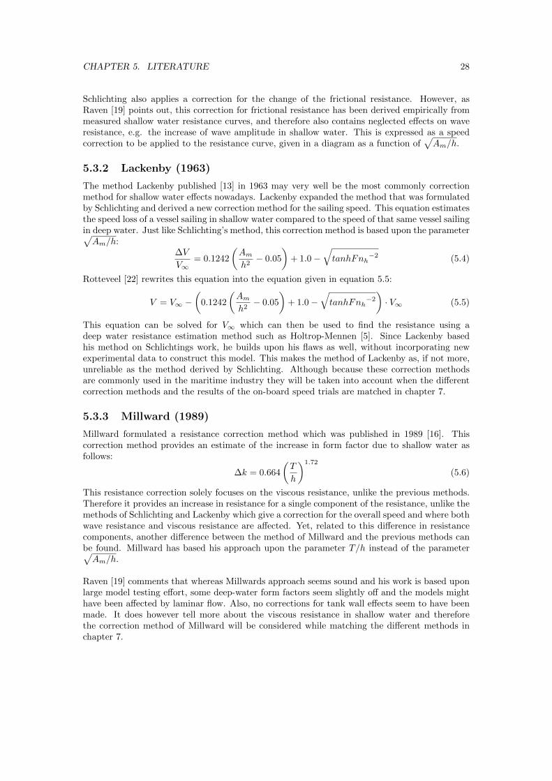
5.3.2 Lackenby (1963)
The method Lackenby published [13] in 1963 may very well be the most commonly correctionmethod for shallow water effects nowadays. Lackenby expanded the method that was formulatedby Schlichting and derived a new correction method for the sailing speed. This equation estimatesthe speed loss of a vessel sailing in shallow water compared to the speed of that same vessel sailingin deep water. Just like Schlichting’s method, this correction method is based upon the parameter√Am/h:
∆V
V∞= 0.1242
(Am
h2− 0.05
)+ 1.0−
√tanhFnh
−2 (5.4)
Rotteveel [22] rewrites this equation into the equation given in equation 5.5:
V = V∞ −(
0.1242
(Am
h2− 0.05
)+ 1.0−
√tanhFnh
−2)· V∞ (5.5)
This equation can be solved for V∞ which can then be used to find the resistance using adeep water resistance estimation method such as Holtrop-Mennen [5]. Since Lackenby basedhis method on Schlichtings work, he builds upon his flaws as well, without incorporating newexperimental data to construct this model. This makes the method of Lackenby as, if not more,unreliable as the method derived by Schlichting. Although because these correction methodsare commonly used in the maritime industry they will be taken into account when the differentcorrection methods and the results of the on-board speed trials are matched in chapter 7.
5.3.3 Millward (1989)
Millward formulated a resistance correction method which was published in 1989 [16]. Thiscorrection method provides an estimate of the increase in form factor due to shallow water asfollows:
∆k = 0.664
(T
h
)1.72
(5.6)
This resistance correction solely focuses on the viscous resistance, unlike the previous methods.Therefore it provides an increase in resistance for a single component of the resistance, unlike themethods of Schlichting and Lackenby which give a correction for the overall speed and where bothwave resistance and viscous resistance are affected. Yet, related to this difference in resistancecomponents, another difference between the method of Millward and the previous methods canbe found. Millward has based his approach upon the parameter T/h instead of the parameter√Am/h.
Raven [19] comments that whereas Millwards approach seems sound and his work is based uponlarge model testing effort, some deep-water form factors seem slightly off and the models mighthave been affected by laminar flow. Also, no corrections for tank wall effects seem to have beenmade. It does however tell more about the viscous resistance in shallow water and thereforethe correction method of Millward will be considered while matching the different methods inchapter 7.

CHAPTER 5. LITERATURE 29
5.3.4 Kamar (1996)
Like Millward, Kamar also focuses on the increase in form factor due to shallow water effects.The correction method Kamar defined was published in 1996 [10]. Kamar derived the followingequation:
∆k = 80.967
(cb ·
B ·√BT
L2OA
)·(T
h
)1.845
(5.7)
It can be found that the main dimensions of the vessel play a big role in Kamar’s method.The method is based on empirical derived expressions for form factors in deep water. Theseexpressions are translated to expressions in shallow water considering model tests of 7 other shipmodels. This correction method of the form factor will nonetheless be considered in chapter 7for it can show whether it specifies the method of Millward regarding the form factor and it canlead to a more clear vision on how a correction method for the Berezina is defined.
5.3.5 Jiang (2001)
Jiang proposes a speed correction which results in an effective speed based on the dynamicsinkage of the vessel. This dynamic sinkage is also known as squat. This resulting effective speedcombines the blockage effect near the vessel, which is important for the viscous resistance, andthe effective depth-effect under the vessel, which is important for the wave effect. The equationthat Jiang has derived for this effective speed is shown in equation 5.8:
VE = V ·
√1+2gzv
V 2
1−zvh
(5.8)
In this equation, zv is the dynamic sinkage of the vessel and can be calculated by using asquat prediction method, of which there are several available. More information on squat effectscan be found in subsection 5.2.5. The effective speed can be used in a deep water resistanceestimation method. This method is the most currently proposed method and gives a differentapproach than the previous explained methods. Jiang states that his method remains valid whenstronger shallow water effects occur. Because of Jiang’s statement and the fact that this methodapproaches shallow water effects in a different way this method is taken into account whenmatching correction methods to the results of the speed trials obtained on board the Berezina.

Chapter 6
Speed Trial Tests
In this chapter the speed trials are being discussed in detail. Section 6.1 contains a descriptionof the speed trials that have to be conducted. In section 6.2 the speed trial results are processedfurther along the guidelines of the document of the ITTC [7].
6.1 Procedure of Conducting Speed Trials
The speed trials with the Berezina will be conducted following the rules and guidelines of theITTC. Part one of the ITTC document ‘Recommended Procedures and Guidelines, Speed andPower Trials’ [7] deals with the preparation and implementation of the speed trials. In prepa-ration the responsibilities are divided among the group members. Jelmar Termorshuizen is re-sponsible for the measurement of the wind speed and direction. Roel van der Bles’ responsibilityis the tracking of time and GPS coordinates. Writing down all of the data from the Berezina’sdashboard i.e. the fuel consumption, heading, waterdepth etc. is the responsibility of Lisa deWaal and lastly the responsibility of overlooking the whole procedure, preparing for the trialsand processing the results lies with Stephanie Tjin-A-Djie.
The idea of the speed trial is to do test runs on different constant sailing speeds and certaindepths and finding the corresponding fuel consumption and engine power. In the previous chap-ter, in section 5.1, the definition of shallow water is given, this is used to determine the depthson which will be tested. This leads to a depth of approximately 2 metres for the shallow waterruns and 6 metres for the deep water runs. During the preparation it was decided that the runswould be done on 3 different speeds going upstream and downstream for both shallow water anddeep water, this gives a total of 12 runs. In every run all of the aforementioned data needs to becatalogued.
The speed trials were conducted on October 14. The deep water runs were conducted on theMooie Nel, a small lake near Haarlem, the Netherlands, of which a map can be found in figure6.1. The shallow water runs were conducted on the Noorder Buiten Spaarne, adjacent to theMooie Nel. On the day the speed trials were conducted some unforeseen factors forced a revisionon the original plan. The Berezina does not have a speedometer and on the waterway whichwill be used for the speed trials there is no current present. Also, it was not possible to sail theexact same route up and down and the depth kept varying on each run. The solution for theseproblems was to not use the current but the wind direction as a reference, not use a constantsailing speed but to keep the rpms of the engine constant and to calculate an average of the
30

CHAPTER 6. SPEED TRIAL TESTS 31
waterdepth over the duration of the run.
All of this led to 6 runs in shallow water and 6 runs in deep water. In both cases 2 runswere done on 2000 rpm, 2 were done on 1500 rpm and 2 were done on 1000 rpm. Of the 2runs per fixed rpm one was done with the wind on the port side and one with the wind on thestarboard side in shallow water. In deep water one of the 2 runs corresponding to a fixed rpmwas done with the Berezina going downwind and the other run with the Berezina experiencingheadwind. In the next section the values of all of the data is catalogued.
Figure 6.1: Map of the Mooie Nel and Noorder Buiten Spaarne, near Haarlem.
6.2 Processing of the Speed Trial Results
In this section the results of the speed trials are processed. In order to process the results ina clear way, the first subsection, subsection 6.2.1 contains some background information and aquick oversight of the steps that need to be followed during the process. In subsection 6.2.2 thesteps given in the first subsection are worked out.
6.2.1 Background Information
According to the ITTC document ‘Recommended Procedures and Guidelines, Speed and PowerTrials’ Part 1 [7] and Part 2 [8] fourteen steps need to be taken to process the results providedby the conducted speed trials on board the Berezina. All appendixes mentioned in this and thefollowing subsection can be found in this same document publicized by the ITTC. However, notall steps will be gone through because not all steps given are relevant to the conducted test asthis document is used for sea trials and the speed trials on board the Berezina are done on inlandwaters. Another argument for not following all of the steps is that some conditions will not beapplicable for the Berezina as she is a much smaller vessel then the vessels for which these trialsare used. This will be further elaborated in subsection 6.2.2. The fourteen given steps containthe following instructions:
1. Derive the average values of each measured parameter for each speed run. The averagespeed is found from the GPS recorded start and end positions of each Speed Run and theelapsed time.
2. Derive the true wind speed and direction for each Double Run by the method described inAppendix B [8].

CHAPTER 6. SPEED TRIAL TESTS 32
3. Correction of power due to resistance increase due to wind.
4. Correction of power due to resistance increase due to waves.
5. Correction of power due to resistance increase due to effect of water temperature andsalinity.
6. Correction of speed due to the effect of shallow water.
7. Correction of power for the difference of displacement and trim from the specific contractualand EEDI (Energy Efficiency Design Index conditions).
8. Correction of the rpm and propulsive efficiency from the load variation model test results.
9. Average the speed, rpm and power over the two runs of each Double Run and over theDouble Runs for the same power setting according to the “mean of means” method [18] toeliminate the effect of current.
10. Check the current speed for each individual speed run by comparing the “mean of means”result at one power setting (step 9) with the results of step 8.
11. Use the speed/power curve from the model test for the specific ship design at the trialdraught. Shift this curve along the power axis to find the best fit with all averaged correctedspeed/power points (from step 9) according to the least squares method [14].
12. Intersect the curve at the specified power to derive the ship’s speed at trial draught in idealconditions.
13. Apply the conversion to other stipulated load conditions according to Appendix A [8].
14. Apply corrections for the contractual weather conditions if these deviate from Ideal Con-ditions.
6.2.2 Speed Trial Results
It can be found that only steps 1 to 3 of the document obtained by the ITTC are applied duringthe process. A justification for this choice is given in this subsection. All steps are discussed oneby one. Table 6.1 gives an oversight of the power and torque for the rpms used during the speedtrials, according to the curve shown in figure A.1 in Appendix A :
Rpm Power Torque[kW] [Nm]
2000 52 2501500 32 1951000 12 130
Table 6.1: Power and torque according to Volkswagen Marine. [26]
According to the first step, the average values of each measured parameter have to be derived,for each speed run. The results are shown in table 6.2. Run 1 to run 6 are done in shallow water,run 7 to run 12 are done in deep water. Written in brackets is the wind direction. SB representswind coming from starboard, likewise PS stands for portside. DW means that the Berezina wassailing downwind, HW represents sailing headwind.

CHAPTER 6. SPEED TRIAL TESTS 33
Depth Speed Wind Revs Heading PWG Fuel[m] [kn] speed [rpm] [deg] [%] consumption
[m/s] [l/h]Run 1 (PS) 2.25 6.44 7.5 2000 231 37 8.8Run 2 (SB) 2.35 7.1 4.3 2000 41 37 9Run 3 (PS) 2.55 5.13 8 1500 228 23 3.7Run 4 (SB) 2.55 5.43 4.3 1500 37 24 3.8Run 5 (PS) 2.15 3.4 5.6 1000 230 10 1.5Run 6 (SB) 2.05 3.99 4.2 1000 42 10 1.4Run 7 (DW) 6.05 7.34 2 2000 350 36 7.4Run 8 (HW) 6.25 7.04 10.2 2000 172 36 7.6Run 9 (DW) 6.15 5.69 2.8 1500 352 23 3.4Run 10 (HW) 6.15 5.47 9 1500 174 23 3.4Run 11 (DW) 6.45 4.09 4.1 1000 351 10 1.4Run 12 (HW) 6.55 3.41 9.1 1000 178 10 1.4
Table 6.2: Average values of the measured parameters during speed trials.
Step 2 contains a derivation of true wind speed and direction. In figures 6.2 to 6.7 the “Averagingprocess for the true wind vectors” according to Appendix B1 [8] are given. These figures showthe following vectors as the average of 2 runs:
� Vn: Ship movement vector at run n.
� VWRn: Measured relative wind vector at run n.
� UAZ : Averaged true wind vector.
Appendix B2 “Correction for the height of the anemometer” [8] will not be used because oneof the variables must come from wind tunnel tests and these were not conducted for the Berezina.
In step 3 the increase of resistance due to wind is calculated according to Appendix C andparagraph 4.3.1 of ITTC- Recommended Procedures and Guidelines Part 2. In this appendix aregression equation based on model tests is given, this equation was created by Fujiwara et al [3]and is defined as follows:
CAA = CLF cosψWR+CXLI
(sinψWR −
1
2sinψWRcos
2ψWR
)sinψWRcosψWR+CALF sinψWRcos
3ψWR
(6.1)CAA is the wind resistance coefficient and the calculated element in this equation. The values ofCLF , CXLI and CALF can be calculated for 0 ≤ ψWR ≤ 90◦ with the following euations:
CLF = β10 + β11AY V
LOAB+ β12
CMC
LOA(6.2)
CXLI = δ10 + δ11AY V
LOAHBR+ δ12
AXV
BHBR(6.3)
CALF = ε10 + ε11AOD
AY V+ ε12
B
LOA(6.4)
The non-dimensional parameters are provided by table 6.3.

CHAPTER 6. SPEED TRIAL TESTS 34
ji 0 1 2 3 4
βij 1 0.922 -0.507 -1.162 - -2 -0.018 5.091 -10.367 3.011 0.341
δij 1 -0.458 -3.245 2.313 - -2 1.901 -12.727 -24.407 40.310 5.481
εij 1 0.585 0.906 -3.239 - -2 0.314 1.117 - - -
Table 6.3: Non-dimensional parameters for components of the wind resistance coefficient. [3]
CAA is now used to calculate the resistance change due to the wind, RAA. The equation for RAA
is:
RAA =1
2· ρair · V 2
WR · ψWR ·AXV · CAA (6.5)
In this equation AXV represents the area of maximum transverse section that is exposed to thewind, which has a value of 34.394 m2. VWR is the relative wind speed and ψWR is the relativewind direction. The density of air, ρair is set at 1.225 kg/m3.
An approximation of ψWR is measured during the speed trial tests and corrected accordingto step 2 of this process. CAA and RAA are calculated for various runs and given in table 6.5.Again, in this table SB represents wind coming from starboard, PS stands for portside. DWdownwind, HW represents the Berezina sailing headwind. The particular components needed forcalculating CAA and RAA are given in table 6.4. The wind for a set of two runs comes from thesame direction. This means that the values for the both runs are identical. For run 12 this is alittle different for the value is the same but in another directino. This is because a ship has theopposite effect when sailing downwind than the effect it experiences when sailing headwind.
LOA [m] 20.6 β10 0.992 CLF 0.608B [m] 4.59 β11 -0.507CMC [m] 2.295 β12 -1.162 CXLI -1.930AY V [m2] 4.394 δ10 -0.458AXV [m2] 3.856 δ11 -3.245 CALF 0.0826HBR [m] 2.36 δ12 2.313AOD [m2] 8.325 ε10 0.585
ε11 0.906ε12 -3.239
Table 6.4: Calculated components of CAA.
Step 4 contains a correction for the waves that are present during the speed runs. However, atthe day of conducting the speed trials hardly any waves were present so this step will not beneeded.
The fifth step stipulates a correction of the ship due to the salinity of the water and the temper-ature of the water. There was no way to determine the temperature of the water and the salinityof the water so this correction was declared irrelevant. Also, it may be irrelevant because thetrials were obtained on inland waters where the water is fresh instead of salt and the guidelinesare assuming the water to be fresh.

CHAPTER 6. SPEED TRIAL TESTS 35
Run ψWR [◦] cos ψWR sin ψWR CAA VWR [m/s] RAA [N]Run 1 (PS) 44 0.719 0.695 -0.0379 7.5 -221.6Run 2 (SB) 8 0Run 3 (PS) 47.5 0.676 0.737 -0.118 5.6 -413.4Run 4 (SB) 4.3 0Run 5 (PS) 44 0.719 0.695 -0.0379 4.3 -72.85Run 6 (SB) 4.2 0Run 7 (DW) 9 0.988 0.156 0.589 2 50.09Run 8 (HW) 2.8 0Run 9 (DW) 7 0.993 0.122 0.599 4.1 166.5Run 10 (HW) 10.2 0Run 11 (DW) 5.5 0.995 0.0958 0.604 9 635.7Run 12 (HW) 9.1 0
Table 6.5: Calculation of CAA and RAA.
The ITTC- Recommended Procedures and Guidelines, Part 2 uses the method by Lackenby forthe effects of shallow water which should be applied according to step 6. Because this methodwill be used separately in this research project to provide the effects of shallow water this willnot be used during the processing of the conducted speed trials. Here, no effects for shallowwater will be used because the speed trials will be placed next to the effects as formulated byLackenby, Schlichting, Jiang et cetera so if the method by Lackenby is used here, comparing withother effects will give invalid values.
Step 7 depicts a correction of power for the difference of displacement and trim from the stipu-lated contractual and EEDI conditions. There are no contractual and EEDI conditions for theBerezina so this step is regarded as irrelevant.
Step 8 encloses correction of the rpm and propulsive efficiency from the load variation model testresults. No load variation model tests were done for the Berezina so this step will not be takeninto account.
According to step 9 the speed, rpm and power over two runs should be averaged. The speed trialis corrected for the current but on the Mooie Nel, the waterway where the trials were conducted,no current was present. This step will not be followed. Likewise, the steps 10 to 12 will not befollowed as they are connected to step 9.
The second-to-last step, step 13, corresponds with Appendix A [8]. In this appendix ballastspeed/power test results and load conditions are applied. The Berezina is not a cargo ship,therefore step 13 is not relevant to the results of the Berezina.
Finally, step 14 corresponds with a deviation in weather conditions from the contractual condi-tions to Ideal Conditions. In this case no contractual conditions were given so this step is skippedas well.

CHAPTER 6. SPEED TRIAL TESTS 36
Figure 6.2: Relative wind of runs 1 and 2.
Figure 6.3: Relative wind of runs 3 and 4.

CHAPTER 6. SPEED TRIAL TESTS 37
Figure 6.4: Relative wind of runs 5 and 6.
Figure 6.5: Relative wind of runs 7 and 8.

CHAPTER 6. SPEED TRIAL TESTS 38
Figure 6.6: Relative wind of runs 9 and 10.
Figure 6.7: Relative wind of runs 11 and 12.

Chapter 7
Matching of Literature and SpeedTrial Tests
In this chapter the literature will be compared with the speed trial results to find the best shallowwater correction method for the Berezina. In order to do this firstly the theoretical deep waterresistance of the Berezina is calculated in section 7.1. After this the method for power estimationand the determination of the needed effeciences are discussed in section 7.2, after which in section7.3 the wind correction for the speed trials can be applied. In section 7.4 the deep water speedtrial results are compared to the theoretical deep water resistance, and in section 7.5 the shallowwater speed trials are compared with the different shallow water correction methods. Finally insection 7.6 a conclusion is drawn for the most appropriate shallow water correction method forthe Berezina.
7.1 Theoretical Deep Water Resistance
In this section the decomposition of the Berezina’s total resistance in deep water is described.The results from this calculation are used to verify the results from the deep water speed trialmeasurements on board the Berezina. The most common methods to determine a vessels resis-tance are model testing and statistical analysis. Since no scale model of the Berezina is availableand the construction of such a model does not fit in the scope of this research project, the choicehas been made to use statistical analysis methods to predict the Berezina’s deep water resistance.
There are numerous statistical methods to predict a vessel’s resistance, but not every predic-tion method is applicable for the Berezina. There are methods specified for seagoing vessels,large displacement vessels, small displacement vessels, naval vessels, high speed planing vessels,multihull vessels, et cetera. Since the Berezina is a relatively small tug boat, the focus of thissection is on the resistance prediction methods for small displacement vessels. The discussedmethods are the Holtrop & Mennen method [5] [17] in subsection 7.1.1, because of its largevariety of vessels and the Van Oortmerssen method in subsection 7.1.2, because this method isspecially focused on small displacement vessels. Subsection 7.1.3 contains a resistance predictionaccording to both prediction methods. Finally the conclusions will be drawn about what methodis best applicable to determine the Berezina’s resistance in subsection 7.1.4.
39

CHAPTER 7. MATCHING OF LITERATURE AND SPEED TRIAL TESTS 40
7.1.1 Holtrop & Mennen Method
The Holtrop & Mennen method is based on the results of numerous model tests and real timeresistance measurements. Although this method is based on seagoing vessels, due to the largevariety of vessels (see table 7.1), it should be possible to make an accurate resistance predictionfor the Berezina. This method provides a calculation of the total resistance of a vessel sailingin deep water, the effects of sailing in shallow water on the vessel’s resistance not taking intoaccount. To achieve reliable results a lot of vessel-particular input is required as discussed insubsection 7.1.3.
Before this method can be used to predict the Berezina’s resistance, it should be checked ifthis method is applicable for the Berezina. From the model testing results some limitations canbe raised, see table 7.1. The hull form parameters found for the Berezina are listed in table 7.2.It shows that the Berezina, mostly, fits in the ‘Fishing Vessels, Tugs’ category. However, theB/T ratio of the Berezina does not fit in. Therefore the method’s reliability is questionable forthe Berezina.
Ship Type L/B B/T cp Fnmax
Tankers, Bulk Carriers 5.1 < L/B < 7.1 2.4 < B/T < 3.2 0.73 < cp < 0.85 0.24General Cargo 5.3 < L/B < 8.0 2.4 < B/T < 4.0 0.58 < cp < 0.72 0.30Fising Vessels, tugs 3.9 < L/B < 6.3 2.1 < B/T < 3.0 0.55 < cp < 0.65 0.38Container Ships, Frigates 6.0 < L/B < 9.5 3.0 < B/T < 4.0 0.55 < cp < 0.67 0.45Various 6.0 < L/B < 7.3 3.2 < B/T < 4.0 0.56 < cp < 0.75 0.30
Table 7.1: Limitations to the Holtrop & Mennen method and variety in vessel types. [17]
7.1.2 Van Oortmerssen Method
The Van Oortmerssen method focuses on small displacement vessels such as tug boats, fishingvessels et cetera. The method is based on results from various model tests. Due to the scope ofthe model tests this method is only applicable [25] for vessels with limited dimensions as shownin table 7.2. As can be found in the table, the Berezina’s specifications match the limitations forthis method so the method should provide a reliable resistance prediction for the Berezina.
Parameter Limitations Berezinamin max
LWL [m] 8.0 80 19.375O [m3] 5.0 3000 49.73L/B 3.0 6.2 4.05B/T 1.9 4.0 3.53cp 0.50 0.73 0.901cm 0.70 0.97 0.77α 10◦ 46◦ 30◦
Fn 0 0.50 0.38
Table 7.2: Limitations to the Van Oortmerssen method compared with the Berezina’s parameters.[25]
CHAPTER 7. MATCHING OF LITERATURE AND SPEED TRIAL TESTS 41
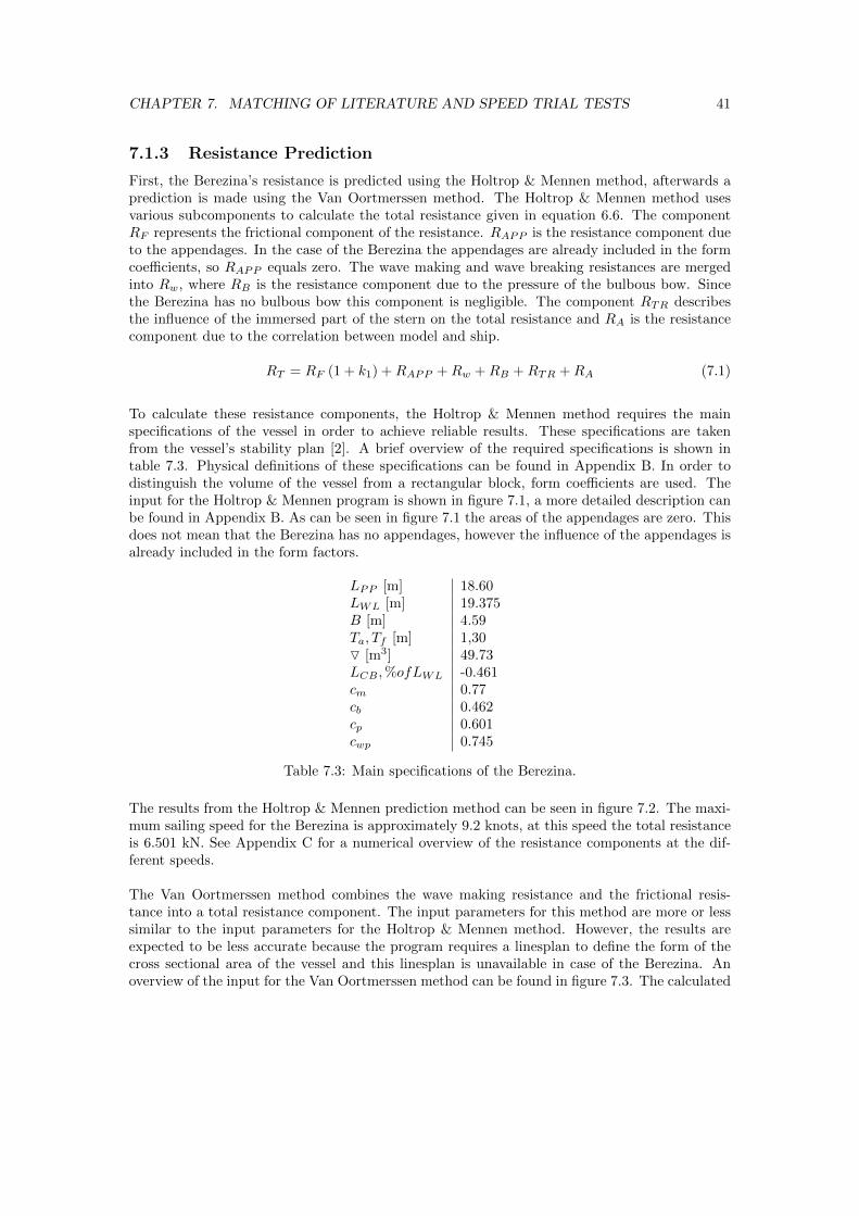
7.1.3 Resistance Prediction
First, the Berezina’s resistance is predicted using the Holtrop & Mennen method, afterwards aprediction is made using the Van Oortmerssen method. The Holtrop & Mennen method usesvarious subcomponents to calculate the total resistance given in equation 6.6. The componentRF represents the frictional component of the resistance. RAPP is the resistance component dueto the appendages. In the case of the Berezina the appendages are already included in the formcoefficients, so RAPP equals zero. The wave making and wave breaking resistances are mergedinto Rw, where RB is the resistance component due to the pressure of the bulbous bow. Sincethe Berezina has no bulbous bow this component is negligible. The component RTR describesthe influence of the immersed part of the stern on the total resistance and RA is the resistancecomponent due to the correlation between model and ship.
RT = RF (1 + k1) +RAPP +Rw +RB +RTR +RA (7.1)
To calculate these resistance components, the Holtrop & Mennen method requires the mainspecifications of the vessel in order to achieve reliable results. These specifications are takenfrom the vessel’s stability plan [2]. A brief overview of the required specifications is shown intable 7.3. Physical definitions of these specifications can be found in Appendix B. In order todistinguish the volume of the vessel from a rectangular block, form coefficients are used. Theinput for the Holtrop & Mennen program is shown in figure 7.1, a more detailed description canbe found in Appendix B. As can be seen in figure 7.1 the areas of the appendages are zero. Thisdoes not mean that the Berezina has no appendages, however the influence of the appendages isalready included in the form factors.
LPP [m] 18.60LWL [m] 19.375B [m] 4.59Ta, Tf [m] 1,30O [m3] 49.73LCB ,%ofLWL -0.461cm 0.77cb 0.462cp 0.601cwp 0.745
Table 7.3: Main specifications of the Berezina.
The results from the Holtrop & Mennen prediction method can be seen in figure 7.2. The maxi-mum sailing speed for the Berezina is approximately 9.2 knots, at this speed the total resistanceis 6.501 kN. See Appendix C for a numerical overview of the resistance components at the dif-ferent speeds.
The Van Oortmerssen method combines the wave making resistance and the frictional resis-tance into a total resistance component. The input parameters for this method are more or lesssimilar to the input parameters for the Holtrop & Mennen method. However, the results areexpected to be less accurate because the program requires a linesplan to define the form of thecross sectional area of the vessel and this linesplan is unavailable in case of the Berezina. Anoverview of the input for the Van Oortmerssen method can be found in figure 7.3. The calculated

CHAPTER 7. MATCHING OF LITERATURE AND SPEED TRIAL TESTS 42
values for the total resistance for this method are shown in figure 7.4. The graph shows thatthe total resistance at a speed of 9.2 knots is equal to 6.885 kN. A numerical overview of theresistance components according to the Van Oortmerssen method is also given in Appendix C.
Figure 7.1: Input for the Holtrop & Mennen resistance method.
Figure 7.2: Results from the Holtrop & Mennen resistance method.
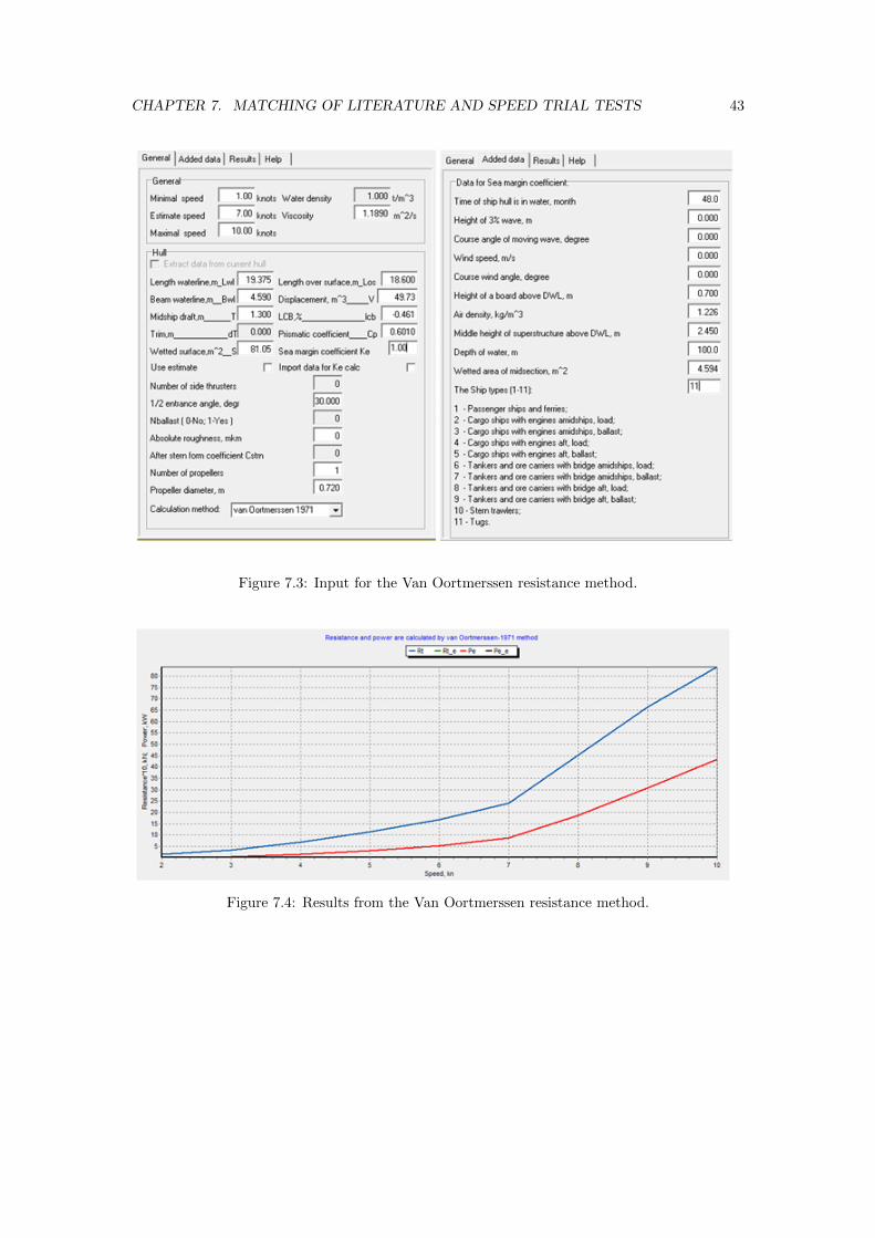
CHAPTER 7. MATCHING OF LITERATURE AND SPEED TRIAL TESTS 43
Figure 7.3: Input for the Van Oortmerssen resistance method.
Figure 7.4: Results from the Van Oortmerssen resistance method.

CHAPTER 7. MATCHING OF LITERATURE AND SPEED TRIAL TESTS 44
7.1.4 The Berezina’s Resistance
When the results of both methods are compared to each other as shown in figure 7.5 it canbe seen that the total resistance curves have a similar slope up to a sailing speed of 7 knots,therefore the methods seem reliable to determine the Berezina’s resistance up to 7 knots. Whenthe speed increases further, the results of both methods start to deviate from each other. TheVan Oortmerssen total resistance curve starts to approach a linear function, where the Holtrop& Mennen total resistance curve continues to follow a polynomial function.
When the speed increases, the effect of the wave making and wave breaking resistance on the to-tal resistance becomes more relevant. The increase in wave making and wave breaking resistanceexceeds the increase in frictional resistance at higher speeds, so the expected total resistancecurve for higher speeds is a polynomial function.
Since the Holtrop & Mennen curve starts to follow a polynomial function, where the Van Oort-merssen curve starts to approach a linear function, the Holtrop & Mennen method seems tobe the best approach of reality for the two methods. Therefore, the choice is made to use theHoltrop & Mennen results (see Appendix C) from this point on.
Figure 7.5: Results from the Holtrop & Mennen- and the Van Oortmerssen resistance methods.

CHAPTER 7. MATCHING OF LITERATURE AND SPEED TRIAL TESTS 45
7.2 Power Estimation
To compare the amount of consumed fuel for the normal sailing condition and the adapted sail-ing speed condition, a correlation between the measured resistance and the fuel consumptionhas to be found. The method used to correlate the measured resistance of the vessel to the fuelconsumption of the engine can be found in literature [11]. A brief overview of the calculationsthat have to be performed is given in this section.
The first step in the process is to calculate the effective towing power. The effective towingpower is the power that is required to move the vessel with a constant speed, see equation 7.2.
PE = RT · VS (7.2)
In order to calculate the thrust power, the influences of the thrust deduction and the vessels wakeon the power needed to move the ship have to be determined. These influences of the thrustdeduction and the wake factor on the power are combined in the hull efficiency. Due to theseinfluences in the water flow behind the ship the effective towing power is not equal to the thrustpower. The next equation is valid for the hull efficiency.
ηH =PE
kp · PT=
1− t1− w
(7.3)
Both the thrust deduction factor and the wake factor are known from the Holtrop & Mennenresistance prediction results. The Berezina’s hull efficiency exceeds one and the vessel has onlyone propeller (kp=1), so the effective towing power is larger than the thrust power.
When the open water conditions for the propeller are known, the power delivered to the propelleras torque can be calculated. The open water efficiency describes the ratio between the powerneeded to move the ship and the power the propeller delivers without interference of the vessel.
The open water efficiency is a propeller specific parameter. Since there is not much informationavailable about the Berezina’s propeller, the open water efficiency is determined using the pro-peller design software: ‘Propcalc’. The known parameters for the Berezina’s propeller are theP/D ratio, diameter and the number of blades. The PropCalc program provides a tool to matcha standard propeller to the Berezina’s propeller, see Appendix D for the details of this process.
With the open water efficiency known, the open water power for the Berezina’s propeller can becalculated:
ηO =PT
PO(7.4)
The open water power in combination with the number of revolutions the propeller has to maketo achieve the required thrust are needed to calculate the torque delivered to the propeller:
Q =PO
2π · np(7.5)
The number of revolutions the propeller has to make is linearly proportional to the sailing speed,as can be seen in equation 7.6.
np = c3 · VS (7.6)
Since the correlation between the number of revolutions and the sailing speed is linearly pro-portional, the factor c3 has to be constant. The number of revolutions related to the maximum

CHAPTER 7. MATCHING OF LITERATURE AND SPEED TRIAL TESTS 46
sailing speed is known, so for this situation the c3 factor can be calculated. This constant factoris needed to determine the number of revolutions for each sailing speed.
The relative rotative efficiency describes the effect of the incoming disturbed water flow onthe performance of the propeller, when compared to the open water situation. Therefore therelative rotative efficiency can be written as the ratio between the open water power and thepower delivered by the propeller, resulting in the following equation:
ηR =PO
PP=
2π ·Q · np2π ·Mp · np
(7.7)
A common range of values for the relative rotative efficiency is between 0,98 and 1,02 [11]. Therelative rotative efficiency for the current propeller is calculated to be 1,02 according to Helm [24],who developed a method where he focused on small vessels. After simplification the remainingequation for the relative rotative efficiency can be found:
ηR =Q
Mp(7.8)
Since the theoretical torque and the open water power are calculated in an earlier stage of theprocess, the relative rotative efficiency is determined to be equal to one, the propeller power andthe related propeller torque Mp can be calculated.
Since the required power and torque for the propeller are determined, the focus changes tothe rest of the drivetrain. The drivetrain of a vessel consists of an engine, gearbox, drive shaftand finally the propeller.
In the previous section the focus was on the propeller and the influence of the incoming/outgoingwater flow. From this point on, the focus will be on the transmission of torque and rotation fromthe engine to the propeller. Therefore, the efficiency of the drive shaft has to be determined.Transmission of energy is often not without dissipation losses. In this specific case shaft lossesare taken account for by means of the shaft efficiency.
ηS =Pp
PS(7.9)
Typical values for the shaft efficiency are ranged between 0,99 and 0,995 [11]. Since the Berez-ina’s engine is located in the aft of the vessel, the drive shaft is small. Where a shaft efficiencyof 0,99 could be used for large vessels with relatively long shafts, the shaft efficiency for theBerezina is determined to be 0,995.
The power delivered to the transmission shaft is called the shaft power. The shaft power isequal to the for the shaft losses adapted propeller power. When the shaft power is determinedthe related shaft torque can be calculated. The shaft power is equal to the shaft torque timesthe propeller revolutions.
PS = 2π ·MS · np (7.10)
The second stage of the transmission process from engine to propeller is the gearbox. Thegearbox reduces the engine speed to a matching propeller speed. To account for the losses in thegearbox the gearbox efficiency has been raised. This efficiency describes the losses between thepower delivered by the prime mover and the power delivered to the drive shaft, as can be seenin equation 7.11 where ke is the number of installed engines. Common values for the gearbox

CHAPTER 7. MATCHING OF LITERATURE AND SPEED TRIAL TESTS 47
efficiency are 0,98 or 0,99 for simple gearboxes and 0,95 to 0,97 for more complex gearboxes [11].The simplicity of a gearbox is dependent on the number of reduction stages in the gearbox. Inthe case of the Berezina a simple gearbox is used, so the efficiency is set to a value of 0,99.
ηGB =PS
ke · PB(7.11)
When the gearbox efficiency is known, the power delivered by the prime mover can be calculated.The generated power is equal to the shaft power adapted for the gearbox losses.
At last the engine’s delivered torque MB can be calculated with equation 7.12:
MB =PB
2π · ne(7.12)
The final step is to calculate the amount of injected fuel per second, related to the delivered power.In combination with the specific fuel consumption, which is given in the engine specifications[26], the amount of injected fuel can be calculated:
mf = sfc · PB (7.13)
The efficiencies and factor c3 assumed for the calculation regarding the engine of the Berezinaare given in table 7.4. An overview of the output of the calculation can be found in appendix E
ηH 1.04ηO 0.494ηR 1.02ηS 0.995ηGB 0.99c3 3.42
Table 7.4: Efficiencies and constant assumed for the Berezina’s engine.
7.3 Correction of the Speed Trial Results
In the previous chapter the correction for the wind has been calculated. In this section the windcorrection will be taken into account when calculating the resistance the Berezina experiencesduring the speed trials. The speed trial measurements include values for the depth of the water,the fuel consumption, the wind speed, the sailing speed, the heading and the rpm’s. With table6.1 the brake power corresponding to the used rpm’s can be found. By using the method, asexplained in section 7.2, the effective power corresponding with the brake power can also befound. By using equation 7.2 the resistance for each of the runs can be found. Table 7.6 showsthe values for all the aforementioned parameters and corrects for the wind resistance to find thetotal resistance the Berezina experiences during the speed trials.

CHAPTER 7. MATCHING OF LITERATURE AND SPEED TRIAL TESTS 48
Figure 7.6: Corrected power and resistance for the Berezina’s speed trial results.
7.4 Speed Trial Results Compared to Holtrop & MennenResults
In order to validate the results of the speed trials, the results are to be compared with the totalresistance curve as obtained from the Holtrop & Mennen resistance prediction method. Since theHoltrop & Mennen resistance prediction method is purely based on deep water conditions, onlythe results from the deep water speed trials are discussed in this section. The results from thespeed trials, corrected for influences of the wind, can be found in table 7.6. A complete overviewof the Holtrop & Mennen results, as discussed in section 7.1, can be found in appendix C. Tocompare the results from both the speed trials and Holtrop & Mennen, the results are plottedin figure 7.7.
Figure 7.7: Speed trials and Holtrop & Mennen resistance values.

CHAPTER 7. MATCHING OF LITERATURE AND SPEED TRIAL TESTS 49
As can be seen in the figure, there is a significant deviation between the results from the speedtrials and the results from the theoretical calculation. Table 7.5 shows the numerical values forboth methods, so a ratio between the two can be calculated. According to these results, it isclear that the ratio between the speed trial results and the Holtrop & Mennen results decreaseswhen the sailing speed increases.
VS Rcorrected RHM Rcorrected/RHM
[kn] [kN ] [kN ]3,41 2,53 0,50 5,114,09 3,27 0,70 4,685,47 5,11 1,27 4,025,69 5,24 1,39 3,767,04 6,41 2,57 2,497,34 6,25 3,01 2,08
Table 7.5: Numerical values and ratio of the Van Ootmerssen and the Holtrop & Mennen method.
An explanation for this phenomenon can be found in the decomposition of the resistance. Thetotal resistance can be divided into a wave making & breaking part and a viscous part. Asdiscussed in chapter 7.1.3, the effect of the wave making resistance and wave breaking resistancebecomes more relevant at high sailing speeds and starts to exceed the effect of the viscous resis-tance. However, for low speeds the viscous (frictional) resistance has the biggest impact on thetotal resistance.
Since the deviation between the speed trial results and the theoretical resistance values is largestfor low speeds, it is expected that the frictional resistance component as calculated with theHoltrop & Mennen method is too small for the Berezina’s situation. The Holtrop & Mennenmethod is designed to predict the resistance of a vessel during its first trial run, which means thatthe assumption is made that the influence of the vessel’s hull roughness on the total resistanceis small.
The hull roughness of the Berezina, built in 1908, can not be expected to satisfy this crite-rion. Another assumption of a first trial run is that the hull and propeller of the vessel are clean.This is certainly not the case for the Berezina. So there are multiple reasons [6] to expect whythe frictional resistance component should be higher than calculated with the Holtrop & Mennenmethod:
� Biological
– Macro biological, animal and weed fouling
– Micro biological, slime fouling
� Physical
– Macro physical, plate waviness, plate laps, mechanical damage, corrosion, rivets, etcetera.
– Micro physical, steel profiles, minor corrosion, condition of coating
The frictional resistance component can be described using equation 7.14 where CF is the fric-tional resistance coefficient. Since the other parameters are constant, the frictional coefficientmust become higher to match the Holtrop & Mennen resistance with the speed trial results.

CHAPTER 7. MATCHING OF LITERATURE AND SPEED TRIAL TESTS 50
To give an indication of the influence of the frictional coefficient on the total resistance, thetotal resistance has been plotted in figure 7.8 for various values for CF . The friction coefficienthas been raised by multiplication of the original value.
RF =1
2· ρ · S · V 2
S · CF (7.14)
Figure 7.8: Speed trial resistances compared with Holtrop & Mennen resistance curves, correctedfor different values of CF .
From the figure it can be seen that in compliance with the speed trial data points the resistancecurves for the 3 · CF and even 4 · CF give the best approximation for the Berezina. The mea-surement tools all have their error margins which are not taken into account in these points. Itis expected that when these error margins are taken into account, the 1.5 · CF line is the bestapproximation of reality, and therefore this resistant curve is used for further calculations in thisreport.
7.5 Applying Shallow Water Correction Methods
In this section the shallow water correction are applied to the results of the speed trials on-board the Berezina. Subsection 7.5.1 contains a correction by Schlichting’s method, subsection7.5.2 covers a correction by Lackenby’s method. In subsection 7.5.3 the correction by Millward’scorrection is applied and in subsection 7.5.4 the correction by Kamar’s method. Lastly, theresults of the correction by JIang’s method are given in subsection 7.5.5.

CHAPTER 7. MATCHING OF LITERATURE AND SPEED TRIAL TESTS 51
7.5.1 Schlichting (1934)
Otto Schlichting developed an equation to predict the shallow water effects, more on this formulacan be found in subsection 5.3.1. This formula is used to calculate the increase in speed ifthe vessel were to sail in deep water. Then that deep water speed is used to determine theresistance according to the Holtrop and Mennen resistance curve. During the speed trials it wasobserved that the depth of the water varies a lot, in each run the average depth of the waterwas documented. The average depth will be calculated for all the shallow water runs and so aconstant depth of the water will be used in the calculation of the corrected speed. The averagedepth that will be used is a depth of 2.3m. Table 7.6 shows the sailing speed, ranging from 1to 10 knots with a stepsize of 0.5 knots, the corresponding Froude number, the correspondingcorrected speed according to Schlichting’s formula and the resulting total resistance. Also theeffective power, the brake power and the fuel consumption are shown in this table.
VS VS Fnh V∞ RT PE PB mf
[kn] [m/s] [kn] [kN ] [kW ] [kW ] [g/h]1 0.514 0.108 1 0.07 0.04 0.07 4.219E-061.5 0.772 0.162 1.5 0.15 0.12 0.24 1.447E-052 1.029 0.217 2 0.26 0.27 0.54 0.00003262.5 1.286 0.271 2.5 0.39 0.51 1.02 6.148E-053 1.543 0.325 3 0.55 0.85 1.71 0.00010313.5 1.801 0.379 3.50 0.73 1.32 2.66 0.00016034 2.058 0.433 4.00 0.94 1.94 3.92 0.00023634.5 2.315 0.487 4.50 1.18 2.73 5.53 0.00033335 2.572 0.542 5.01 1.46 3.76 7.61 0.00045875.5 2.829 0.596 5.520 1.79 5.08 10.27 0.00061916 3.087 0.650 6.059 2.22 6.92 14 0.00084396.5 3.344 0.704 6.616 2.78 9.49 19.2 0.00115707 3.601 0.758 7.219 3.63 13.47 27.24 0.00164207.5 3.858 0.812 7.871 4.88 19.78 40.01 0.00241178 4.116 0.866 8.578 6.31 27.82 56.26 0.00339128.5 4.373 0.921 9.344 8.18 39.26 79.41 0.00478679 4.63 0.975 10.172 11.91 62.26 125.95 0.00759209.5 4.887 1.029 11.063 18.02 102.55 207.47 0.012505810 5.14 1.08 12.02 23.4 144.63 292.6 0.0176373
Table 7.6: Results after correction by Schlichting’s method.

CHAPTER 7. MATCHING OF LITERATURE AND SPEED TRIAL TESTS 52
7.5.2 Lackenby (1963)
In this formula the method differs from that of Schlichting. Lackenby expanded Schlichting’sformula, but Lackenby considers the deep water sailing speed as a known parameter and calculatesa corresponding shallow water speed. Because the speed trials provide the shallow water sailingspeed, the method of Lackenby will be worked out for a speed range of 1-10 knots with steps of0.05. Now the corresponding shallow water speeds will be determined for a range of 1-10 knotswith steps of 0.5 knots and the resulting resistance will be found with help from the Holtrop &Mennen program. For this method the average depth of 2.3m will be used. Table 7.7 shows thedeep water speed corresponding with the shallow water sailing speed and the resulting resistance.
VS V∞ RT PE PB mf
[kn] [kn] [kN ] [kW ] [kW ] [g/h]0.898 1 0.07 0.04 0.07 4.219E-061.348 1.5 0.15 0.12 0.24 1.447E-051.797 2 0.26 0.27 0.54 0.00003262.246 2.5 0.39 0.51 1.02 6.148E-052.695 3 0.55 0.85 1.71 0.00010313.144 3.5 0.73 1.32 2.66 0.00016033.593 4 0.94 1.94 3.92 0.00023634.042 4.5 1.18 2.73 5.53 0.00033334.486 5 1.45 3.73 7.54 0.00045454.921 5.5 1.77 5.02 10.15 0.00061185.338 6 2.17 6.69 13.53 0.00081565.725 6.5 2.65 8.85 17.89 0.00107846.076 7 3.28 11.8 23.87 0.00143886.384 7.5 4.41 15.98 23.33 0.00140636.648 8 5.15 21.21 42.9 0.00258596.868 8.5 6.15 26.56 54.33 0.00327497.048 9 7.4 33.5 67.77 0.00408507.192 9.5 8.71 42.61 86.2 0.00519597.304 10 10.92 56.14 113.56 0.0068451
Table 7.7: Results after correction by Lackenby’s method.

CHAPTER 7. MATCHING OF LITERATURE AND SPEED TRIAL TESTS 53
7.5.3 Millward (1989)
Millward’s method works with a change in the form factor. This will result in a new form factorthat will be used to calculate a new resistance for the vessel. Just as for the other methodsthe depth will be taken at 2.3m. Table 7.8 shows the vessel’s sailing speed in a range of 1-10knots with steps of 0.5 knots, the corresponding resistance in deep water, the old total resistancecoefficient with which the CW can be calculated, the new CF , the new CT and finally thecorrected resistance. In table7.9 the corresponding PE , PB and mf will be shown.
VS VS RDEEP CT 1, 5 · CF (1 + k +4k) CW CT,SHALLOW RSHALLOW
·CF
[kn] [m/s] [kN ] [kN ]1 0.51 0.051 0.0048 0.0046 0.0051 0.00016 0.0086 0.0921.5 0.77 0.107 0.0044 0.0043 0.0048 0.000097 0.0080 0.1932 1.03 0.183 0.0043 0.0041 0.0045 0.000098 0.0076 0.3282.5 1.29 0.278 0.0041 0.0040 0.0044 0.00011 0.0074 0.4963 1.54 0.391 0.0041 0.0039 0.0043 0.00010 0.0072 0.6963.5 1.80 0.520 0.0040 0.0038 0.0041 0.000096 0.0071 0.9274 2.06 0.670 0.0039 0.0037 0.0041 0.00011 0.0069 1.1904.5 2.32 0.842 0.0039 0.0036 0.0040 0.00013 0.0069 1.4875 2.57 1.043 0.0039 0.0036 0.0039 0.00020 0.0068 1.8275.5 2.83 1.287 0.0040 0.0035 0.0039 0.00031 0.0069 2.2216 3.09 1.594 0.0041 0.0035 0.0038 0.00052 0.0070 2.6926.5 3.34 1.986 0.0044 0.0034 0.0038 0.00080 0.0072 3.2597 3.60 2.518 0.0048 0.0034 0.0037 0.0012 0.0076 3.9777.5 3.86 3.277 0.0054 0.0034 0.0037 0.0019 0.0082 4.9358 4.12 4.175 0.0061 0.0033 0.0037 0.0026 0.0088 6.0438.5 4.37 5.057 0.0065 0.0033 0.0036 0.0031 0.0092 7.1479 4.63 6.025 0.0069 0.0033 0.0036 0.0035 0.0096 8.3499.5 4.89 7.375 0.0076 0.0032 0.0036 0.0042 0.0103 9.94410 5.14 9.450 0.0088 0.0032 0.0035 0.0054 0.0114 12.275
Table 7.8: Results after correction by Millward’s method.
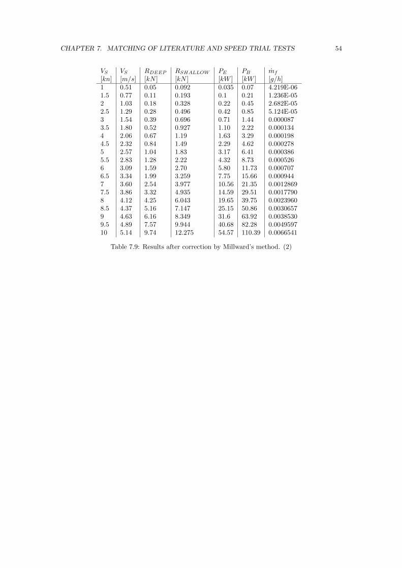
CHAPTER 7. MATCHING OF LITERATURE AND SPEED TRIAL TESTS 54
VS VS RDEEP RSHALLOW PE PB mf
[kn] [m/s] [kN ] [kN ] [kW ] [kW ] [g/h]1 0.51 0.05 0.092 0.035 0.07 4.219E-061.5 0.77 0.11 0.193 0.1 0.21 1.236E-052 1.03 0.18 0.328 0.22 0.45 2.682E-052.5 1.29 0.28 0.496 0.42 0.85 5.124E-053 1.54 0.39 0.696 0.71 1.44 0.0000873.5 1.80 0.52 0.927 1.10 2.22 0.0001344 2.06 0.67 1.19 1.63 3.29 0.0001984.5 2.32 0.84 1.49 2.29 4.62 0.0002785 2.57 1.04 1.83 3.17 6.41 0.0003865.5 2.83 1.28 2.22 4.32 8.73 0.0005266 3.09 1.59 2.70 5.80 11.73 0.0007076.5 3.34 1.99 3.259 7.75 15.66 0.0009447 3.60 2.54 3.977 10.56 21.35 0.00128697.5 3.86 3.32 4.935 14.59 29.51 0.00177908 4.12 4.25 6.043 19.65 39.75 0.00239608.5 4.37 5.16 7.147 25.15 50.86 0.00306579 4.63 6.16 8.349 31.6 63.92 0.00385309.5 4.89 7.57 9.944 40.68 82.28 0.004959710 5.14 9.74 12.275 54.57 110.39 0.0066541
Table 7.9: Results after correction by Millward’s method. (2)

CHAPTER 7. MATCHING OF LITERATURE AND SPEED TRIAL TESTS 55
7.5.4 Kamar (1996)
Kamar’s structure is similar to that of Millward (1989). For this case the depth will also betaken as 2.3m. Table 7.10 and table 7.11 show the results of the calculation.
VS VS RDEEP CT 1, 5 · CF CW CT,SHALLOW RSHALLOW
[kn] [m/s] [kN ] [kN ]1 0.51 0.051 0.005 0.005 0.00016 0.0083 0.0891.5 0.77 0.107 0.004 0.004 0.00010 0.0077 0.1862 1.03 0.183 0.004 0.004 0.00010 0.0074 0.3172.5 1.29 0.278 0.004 0.004 0.00011 0.0072 0.4803 1.54 0.391 0.004 0.004 0.00011 0.0070 0.6743.5 1.80 0.520 0.004 0.004 0.00009 0.0068 0.8964 2.06 0.670 0.004 0.004 0.00011 0.0067 1.1504.5 2.32 0.842 0.004 0.004 0.00013 0.0066 1.4395 2.57 1.043 0.004 0.004 0.00020 0.0066 1.7685.5 2.83 1.287 0.004 0.004 0.00032 0.0066 2.1526 3.09 1.594 0.004 0.003 0.00052 0.0068 2.6096.5 3.34 1.986 0.004 0.003 0.00080 0.0070 3.1637 3.60 2.518 0.005 0.003 0.00124 0.007 3.8687.5 3.86 3.277 0.005 0.003 0.00191 0.0080 4.8118 4.12 4.175 0.006 0.003 0.00259 0.0086 5.9038.5 4.37 5.057 0.007 0.003 0.00306 0.0090 6.9919 4.63 6.025 0.007 0.003 0.00349 0.0094 8.1759.5 4.89 7.375 0.008 0.003 0.00420 0.0101 9.75210 5.14 9.450 0.009 0.003 0.00541 0.0113 12.063
Table 7.10: Results after correction by Kamar’s method.
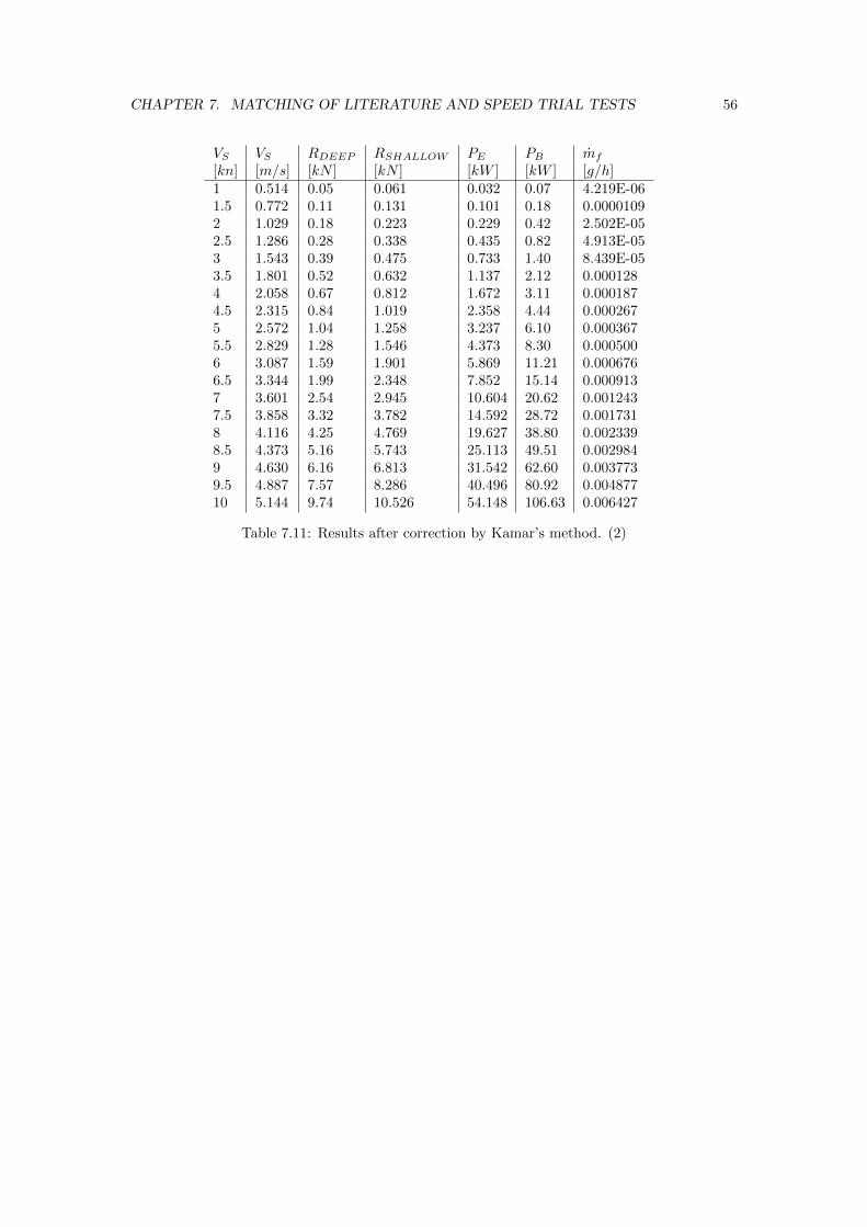
CHAPTER 7. MATCHING OF LITERATURE AND SPEED TRIAL TESTS 56
VS VS RDEEP RSHALLOW PE PB mf
[kn] [m/s] [kN ] [kN ] [kW ] [kW ] [g/h]1 0.514 0.05 0.061 0.032 0.07 4.219E-061.5 0.772 0.11 0.131 0.101 0.18 0.00001092 1.029 0.18 0.223 0.229 0.42 2.502E-052.5 1.286 0.28 0.338 0.435 0.82 4.913E-053 1.543 0.39 0.475 0.733 1.40 8.439E-053.5 1.801 0.52 0.632 1.137 2.12 0.0001284 2.058 0.67 0.812 1.672 3.11 0.0001874.5 2.315 0.84 1.019 2.358 4.44 0.0002675 2.572 1.04 1.258 3.237 6.10 0.0003675.5 2.829 1.28 1.546 4.373 8.30 0.0005006 3.087 1.59 1.901 5.869 11.21 0.0006766.5 3.344 1.99 2.348 7.852 15.14 0.0009137 3.601 2.54 2.945 10.604 20.62 0.0012437.5 3.858 3.32 3.782 14.592 28.72 0.0017318 4.116 4.25 4.769 19.627 38.80 0.0023398.5 4.373 5.16 5.743 25.113 49.51 0.0029849 4.630 6.16 6.813 31.542 62.60 0.0037739.5 4.887 7.57 8.286 40.496 80.92 0.00487710 5.144 9.74 10.526 54.148 106.63 0.006427
Table 7.11: Results after correction by Kamar’s method. (2)

CHAPTER 7. MATCHING OF LITERATURE AND SPEED TRIAL TESTS 57
7.5.5 Jiang (2001)
Literature provides numerous formulae which calculate the dynamic sinkage. The work of Briggs[1] gives an overview of these methods and provides clear criteria for which method works best inparticular cases. The work of Briggs will be worked through step by step to come to a conclusionas to which method fits best with the Berezina and this research project.
� Determining the channel configurationThere are three types of channels according to Briggs. Type 1 is an Unrestricted Channel,type 2 is a Restricted Channel and type 3 is a Canal (see figure 7.9). For the Berezina casethe assumption is made that the only restricted parameter related to the waterway is thewater depth, therefore the ‘unrestricted channel’ type will be used for the calculation.
Figure 7.9: Different channel types, according to Briggs. [1]
The effective width of the waterway can be calculated following equation 7.15:
WEFF =(7.7 + 45(1− C2
wp))·B (7.15)
However, according to the Berezina’s stability plan by Cadhead [2], the cwp is equal to 0.745at a draught of 1.3 m. Substituting this value and the Berezina’s width in the equation forthe effective width of the waterway provides a value for WEFF of 48.8 m.
� Determining the block coefficient, cbThis value is also found in the stability plan provided by Cadhead [2] and is 0.462.
� Determining the water depth- draught coefficient for the different speed trial attempts inshallow waterThese values can be found in table 7.12:
Run Water depth [m] h/T [-]Run 1 (PS) 2.25 1.731Run 3 (PS) 2.55 1.962Run 5 (PS) 2.15 1.654Run 2 (SB) 2.35 1.808Run 4 (SB) 2.55 1.962Run 6 (SB) 2.05 1.577
Table 7.12: Water depth draught coefficients.
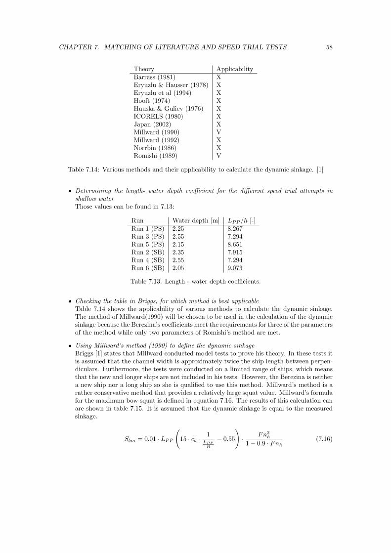
CHAPTER 7. MATCHING OF LITERATURE AND SPEED TRIAL TESTS 58
Theory ApplicabilityBarrass (1981) XEryuzlu & Hausser (1978) XEryuzlu et al (1994) XHooft (1974) XHuuska & Guliev (1976) XICORELS (1980) XJapan (2002) XMillward (1990) VMillward (1992) XNorrbin (1986) XRomishi (1989) V
Table 7.14: Various methods and their applicability to calculate the dynamic sinkage. [1]
� Determining the length- water depth coefficient for the different speed trial attempts inshallow waterThose values can be found in 7.13:
Run Water depth [m] LPP /h [-]Run 1 (PS) 2.25 8.267Run 3 (PS) 2.55 7.294Run 5 (PS) 2.15 8.651Run 2 (SB) 2.35 7.915Run 4 (SB) 2.55 7.294Run 6 (SB) 2.05 9.073
Table 7.13: Length - water depth coefficients.
� Checking the table in Briggs, for which method is best applicableTable 7.14 shows the applicability of various methods to calculate the dynamic sinkage.The method of Millward(1990) will be chosen to be used in the calculation of the dynamicsinkage because the Berezina’s coefficients meet the requirements for three of the parametersof the method while only two parameters of Romishi’s method are met.
� Using Millward’s method (1990) to define the dynamic sinkageBriggs [1] states that Millward conducted model tests to prove his theory. In these tests itis assumed that the channel width is approximately twice the ship length between perpen-diculars. Furthermore, the tests were conducted on a limited range of ships, which meansthat the new and longer ships are not included in his tests. However, the Berezina is neithera new ship nor a long ship so she is qualified to use this method. Millward’s method is arather conservative method that provides a relatively large squat value. Millward’s formulafor the maximum bow squat is defined in equation 7.16. The results of this calculation canare shown in table 7.15. It is assumed that the dynamic sinkage is equal to the measuredsinkage.
Sbm = 0.01 · LPP
(15 · cb ·
1LPP
B
− 0.55
)· Fn2h
1− 0.9 · Fnh(7.16)

CHAPTER 7. MATCHING OF LITERATURE AND SPEED TRIAL TESTS 59
VS VS Fnh Sbm
[kn] [m/s] [−] [m]1 0.514 0.108 0.0031.5 0.772 0.162 0.0072 1.029 0.217 0.0132.5 1.286 0.271 0.0213 1.543 0.325 0.0323.5 1.801 0.379 0.0474 2.058 0.433 0.0664.5 2.315 0.487 0.0915 2.572 0.542 0.1235.5 2.829 0.596 0.1656 3.087 0.650 0.2196.5 3.344 0.704 0.2927 3.601 0.758 0.3907.5 3.858 0.812 0.5298 4.116 0.866 0.7368.5 4.373 0.921 1.066
Table 7.15: Results for the maximum bow squat calculation, using Millward’s equation.
Now that the dynamic sinkage is calculated the formula of Jiang can be used to calculate theeffective speed and the corresponding total resistance. Table 7.16 and table 7.17 show the resultsfor the calculations performed with the Jiang correction method.
VS VS Fnh Measured VE RT
[kn] [m/s] sinkage[m] [kn] [kN ]1 0.514 0.108 0.0028 1.10 0.0871.5 0.772 0.162 0.0067 1.66 0.1842 1.029 0.217 0.0126 2.23 0.3182.5 1.286 0.271 0.0209 2.81 0.4883 1.543 0.325 0.0322 3.40 0.6943.5 1.801 0.379 0.0471 4.01 0.9464 2.058 0.433 0.0664 4.64 1.2514.5 2.315 0.487 0.0913 5.30 1.6385 2.572 0.542 0.1234 6.01 2.1765.5 2.829 0.596 0.165 6.77 2.9656 3.087 0.650 0.219 7.60 4.3386.5 3.344 0.704 0.292 8.55 6.2477 3.601 0.758 0.390 9.69 9.4487.5 3.858 0.812 0.529 11.14 18.4798 4.116 0.866 0.736 13.20 29.488
Table 7.16: Results after correction by Jiang’s method.

CHAPTER 7. MATCHING OF LITERATURE AND SPEED TRIAL TESTS 60
VS VS VE RT PE PB mf
[kn] [m/s] [m/s] [kn] [kN ] [kN ] [g/s]1 0,514 0,566 86,5 0,044 0,090 5,422E-061,5 0,772 0,853 184 0,142 0,287 1,730E-052 1,029 1,146 317,5 0,327 0,660 3,980E-052,5 1,286 1,443 487,5 0,627 1,267 7,639E-053 1,543 1,748 693,5 1,070 2,164 1,304E-043,5 1,801 2,062 946 1,703 3,443 2,075E-044 2,058 2,388 1251 2,574 5,204 3,137E-044,5 2,315 2,729 1638 3,792 7,665 4,620E-045 2,572 3,090 2176 5,597 11,314 6,820E-045,5 2,829 3,480 2965 8,389 16,958 1,022E-036 3,087 3,911 4337,5 13,388 27,063 1,631E-036,5 3,344 4,401 6246,5 20,888 42,222 2,545E-037 3,601 4,984 9447,5 34,021 68,771 4,145E-03
Table 7.17: Results after correction by Jiang’s method. (2)
7.6 Results
Now that all of the values are known for the various methods and the speed trials these canbe compared to each other. This is shown in figure 7.10. This figure depicts the resistance theBerezina experiences and the sailing speed. A depth of 2.3m is taken for all the methods becausethis is the average of all the shallow water runs. According to this figure the method of Jiang isthe best approximation to the speed trial measurements. Knowing this the method of Jiang willbe used in the scenario simulator.
Figure 7.10: Berezina’s resistance-speed curves at h = 2.3m.

Chapter 8
Scenario Simulation
This section describes the design, the development and the results of the scenario simulator thatwas mentioned in section 3.2. In the previous chapters of this report, correction methods wereconsidered which describe the influence of the change in water depth on the resistance of thevessel. These methods have been compared to the speed trial results to check their reliability.The first section of this chapter, section 8.1, contains the working of the simulator, the outcomeof the matching process taken into account. In this simulator several simplifications have beenmade. Section 8.2 covers the results obtained from running the scenario simulator.
8.1 Simulator
This simulator is created as a tool to test the influence of adapting the speed to the water depthon the resistance, and therefore on the amount of injected fuel per route. The main goal of thesimulation is to find an educated answer to the main question of this report. In this section thesimulator itself is discussed, with an overview of the necessary simplifications in subsection 8.1.1an explanation of the inner workings of the simulator in subsection 8.1.2, an in depth look at thespeed advisory in subsection 8.1.3 and the results that are expected in subsection 8.1.4.
8.1.1 Simplifications
To demonstrate the amount of fuel saved for the various simulations, simplifications of reality aretaken into account. Some of the simplifications are a result of the scope of the research project,see section 3.2. The simplifications, as implemented in the model, are stated in the following list.
� Influence of shallow water effects when Fnh > 0.5A distinction between shallow and deep water can be made according to the Froude depthnumber. The definition, as stated in section 5.1, describes that a vessel sails in shallowwater when the Froude depth number exceeds 0.5. Therefore, the model considers a shallowwater condition when the Froude depth number exceeds 0.5 and a deep water conditionwhen the Froude number is lower than 0.5. For the shallow water condition the resistanceis compensated using the shallow water correction method from Jiang.
� Instantaneous speed changesThe instantaneous speed changes are implemented into the simulation model, because thismodel is only used to illustrate the effect of the varying speed at varying water depths.The effects of the acceleration is therefore neglected in this model.
61

CHAPTER 8. SCENARIO SIMULATION 62
� No added resistance effects wind and currentThe speed trial results are corrected for the wind and the effect of the current on thetotal resistance was negligible. The results from the Holtrop & Mennen method are alsofree from wind and current effects, therefore the added effects from wind and current areneglected in the simulations.
� Simulated routeSince no detailed depth charts are available of the waters where the speed trials wereconducted, the choice has been made to simulate various routes. Simulation of these routesis useful to demonstrate the amount of fuel that can be saved. The routes have beencomposed according to the following simplifications:
1. The water depth on the route varies instantaneously.
2. The vessel’s heading is constant and therefore the route is a straight line.
3. The depth on the route is known beforehand.
4. The width of the channel is infinite, therefore bank effects are neglected.
� Deep water resistance from Holtrop & Mennen, compensated for CF
The deep water speed trial resistance and the deep water resistance, as predicted with theHoltrop & Mennen method, deviate from each other. Since this is caused by the influenceof the frictional coefficient, the Holtrop & Mennen resistance a correction has been appliedto the Holtrop & Mennen resistance (see section 7.2). This corrected resistance is used asinput for the model.
� Wake- and thrust deduction factor from Holtrop & Mennen resistance predictionThe wake- and thrust deduction factor are estimated using the Holtrop & Mennen resistanceprediction method. This method uses statistical predicition equations to estimate the wake-and thrust deduction factor [5].
� Shallow water effects corrected for with JiangAs discussed in chapter 7, Jiang’s correction method will be used to correct for the addedresistance effects of sailing in shallow waters.
� Estimated efficiencies for fuel consumption calculationThe method to correlate the measured or predicted resistance to the fuel consumption, asdiscussed in section 7.1, will be implemented in the model. The efficiencies used in thiscalculation process are estimated, since efficiencies are often not included in product guides.
� Speed correction Jiang cannot exceed 15 knotsThe Berezina’s maximum sailing speed is 9.2 knots. The effective speed corresponding tothis maximum speed limit is somewhere around 15 knots, as determined by Jiang.
8.1.2 Inner Workings of the Scenario Simulator
The sailing speed advisory is opened through running the GUI.m file from Matlab. The interfaceof the advisory when initially opened can be seen in figure 8.1. By pressing the button ‘Importroute’ the depth profile of a route can be loaded into the simulation. The desired duration canthen be entered, after which the calculation can be started by pressing the ‘Calculate’ button.After the ‘Calculate’ button is pressed, the following steps take place:

CHAPTER 8. SCENARIO SIMULATION 63
1. The route is loaded into the local workspace
2. The duration is loaded into the local workspace
3. The constants are defined
4. The average speed is calculated
5. The Froude depth number on each interval is calculated
6. The average Froude depth number is calculated
7. The advised speed on each interval is calculated
8. The resistance on each interval for both the average and the advised speed are calculatedIf the Froude depth number on the interval is greater than 0.5, the resistance correction ofJiang is applied.
9. The effective towing power (PE) is on each interval is calculated for both speeds
10. The brake power (PB) on each interval is calculated for both speeds
11. The fuel consumption on each interval is calculated for both speeds
12. The total fuel consumption is calculated for both speeds
13. The total fuel consumptions are compared to see if fuel is saved
14. The fuel consumptions are written into the GUI
15. The depth profile of the route and the average and advised speed on the route are plotted
Figure 8.1: The Graphical User Interface of the simulator.

CHAPTER 8. SCENARIO SIMULATION 64
For an in-depth look, a copy of the code is provided in appendix F. After running the calculations,the results are either plotted or written into the GUI. An example can be seen in figure 8.2.
Figure 8.2: The Graphical User Interface of the simulator after running calculations.
Two graphs are plotted in the GUI. On the left the depth profile of the imported route isdisplayed. The y-axis of this graph is reversed, so that the top of the graph can be seen as thewater surface and the plotted line can be seen as the canal floor. In the graph on the right boththe mean and advised speed are plotted for the whole route. In the top right corner of the GUIthe fuel consumptions and savings can be read. If fuel is saved, the percentage of fuel saved willbe displayed as green text. If fuel is lost, the percentage of fuel lost will be displayed in red text.
8.1.3 Speed Advisory
During step 7 of the step-by-step process outlined in subsection 8.1.2, the advised speed on theroute is calculated. Optimally, this advised speed is optimized for the lowest total fuel con-sumption on the route within the time constraint. This optimization is based on the followinghypothesis:
On a route with different water depths and a constant duration fuel can be saved between thesituation where speed is constant and the situation where speed is varied in such a way that whensailing in relative deep water the speed is increased and when sailing in relative shallow water thespeed is decreased.
The method used to achieve this is sailing on a constant Froude depth number. First, theFroude depth number for each interval with the mean speed is calculated. Then, the meanFroude depth number is calculated. Hereafter, the speed on each interval that must be sailed atto sail at this mean Froude depth number is calculated. This speed is the advised speed.

CHAPTER 8. SCENARIO SIMULATION 65
8.1.4 Expectations
Due to the nature of the speed advisory and the application of the resistance correction above aFroude depth number of 0.5 it is expected that the greatest fuel savings can be achieved whenthe mean Froude depth number of a route approaches 0.5 from below. When the mean Froudedepth number crosses this threshold the shallow water resistance correction will be applied onthe entire route for the advised speed. Fuel savings seem unlikely in this scenario. When themean Froude depth number drops too far below 0.5 only a relative small portion off the voyagewith the mean speed will be in shallow water, which means relative little fuel can be saved whensailing the advised speed, until here too a threshold is crossed and fuel is lost when sailing theadvised speed.
8.2 Results of the Scenario Simulation
In this section the results for four different routes are shown and discussed, with subsection 8.2.1trough subsection 8.2.4 corresponding to route 1 through 4. All routes have a total distance ofa 1000 m. This is sufficient to see notable changes in the total fuel consumed between the meansailing speed and the advised sailing speed. Scaling up these routes would affect the total fuelconsumption, but not the ratio of the fuel saved, and is as such deemed unnecessary.
8.2.1 Route 1
Figure 8.3: Route 1: Constant depth profile.
The first route tested is a route with a constant depth profile, as can be seen in the figure above.As is expected of this route, the simulation shows that the advised speed is the same as the meanspeed, and thusly no fuel is saved or lost in comparison.

CHAPTER 8. SCENARIO SIMULATION 66
8.2.2 Route 2
Figure 8.4: Route 2: A single depth change of 2m.
The second route has a single change in depth. With a length of 1000m and a duration of 400s,the mean speed is 2.5 m/s or 4.86 kn. This route was designed to have a mean Froude depthnumber of 0.4999 at this duration. In this scenario a fuel saving of 41.6 g, or 18.2%, is achieved.
After the mean Froude depth number at 0.4999 with a duration of 400s was achieved the durationwas varied between 260s and 700s, with an irregular time step, in order to identify the relationbetween the mean Froude depth number and the fuel saved in percentages. The results can beseen in graph 8.5:.
As expected, there are fuel savings just below mean Froude depth number 0.5. These existuntil the lower threshold at mean Froude depth number 0.44, after which only losses are encoun-tered. Just above mean Froude depth number 0.5 there are also fuel losses, as was expected.However, above mean Froude depth number 0.63 fuel is again saved. The percentage of fuelsaved steadily climbs, until at a mean Froude depth number of 0.77 the maximum speed of theBerezina is reached.
While the fuel savings at mean Froude depth number 0.63 and above show that when sail-ing at high enough speeds in shallow water it is preferable to increase speeds in the relative deepparts and slow down on the relative shallow parts of the route, it should be noted that the totalfuel consumption skyrockets at these speeds. When sailing at mean Froude depth number 0.7017the percentage fuel saved is close to the percentage when sailing at mean Froude depth number0.4999, while the total fuel consumed has increased with a factor 5 to 955,7g.

CHAPTER 8. SCENARIO SIMULATION 67
Figure 8.5: Route 2: Fuel savings at different mean Froude depth numbers.
Figure 8.6: Route 2: At mean Froude depth number 0.7017.

CHAPTER 8. SCENARIO SIMULATION 68
8.2.3 Route 3
The third route is a route with three different depths. This route, when optimized for a meanFroude depth number at a duration of 400s, saves slightly less fuel than the route with only twodifferent depths, respectively 18.20% and 17.45% (see figure 8.7. When the duration is varied inorder to investigate the relation between mean Froude depth number and fuel savings figure 8.8is found which is very similar to figure 8.5.
Figure 8.7: Route 3: Varying water depth profile.
Figure 8.8: Route 3: Fuel savings at different mean Froude depth numbers.

CHAPTER 8. SCENARIO SIMULATION 69
8.2.4 Route 4
Figure 8.9: Route 4: A single depth change of 10m.
The fourth route has the same depth profile as route 2, with the difference that the relativedeep part of the route is 10m deep instead of 2m. This route clearly show the limitations of theused speed correction method. The mean Froude depth number is greatly influenced by the bigdifference in water depths, and thus the advised speed is different from route 2, resulting in afuel loss on a seemingly very similar route. This scenario shows that the speed advisory worksbest when the depth differences on the route are relatively small.

Chapter 9
Conclusions
The main question of this research is To which extent can the fuel consumption of the Berezinabe reduced, when the vessel’s sailing speed is varied in shallow waters on inland waterways, withrespect to the water depth?. This question has been answered through literature study, speedtrial tests and scenario simulation. In the literature study the works of Schlichting, Lackenby,Millward, Kamar and Jiang were researched and worked out for the Berezina, these scientistsall derived methods that predict the shallow water effects a ship experiences. Speed trial testswere done on the Berezina according to the procedures and guidelines of the ITTC. The averagewater depth of the shallow water speed trial runs is used in the literature study. The speed trialsand literature study were compared and the best method of the literature was chosen as startingpoint of the scenario simulation, this comparison shows that the method of Jiang is closest to thespeed trials. In the scenario simulation different routes with varying water depth will be used asinput and the program will provide a speed advisory for this route as well as the percentage offuel consumption reduction for this route.
The hypothesis states that a reduction of at least 10% will be reached. In the most optimumcase in the scenario simulation the reduction of the fuel consumption is 18.2%, this is more thanstated in the hypothesis and thus it can be said that the hypothesis has been proven.
A series of sub-questions have been formulated to help adequately answer the main question.These were answered throughout the report and will be shortly answered here.
1. When is water shallow?Research concludes that water is shallow when the Froude depth number is more than 0.5.See section 5.1 for detailed information.
2. How does the water depth influence the resistance of the vessel?When a vessel sails in shallow water it experiences extra sinkage and trim, a differentpressure distribution along the hull which leads to a different form factor and viscous flowand the squat effect. See section 5.2 for detailed information about the effects that a shipexperiences when sailing in shallow water.
3. How can a correction, due to the variation in water depth, in the vessels resistance becalculated?Schlichting, Lackenby and Jiang have formulated methods that calculate a corrected sailingspeed in deep water that corresponds with the sailing speed in shallow water. The deepwater sailing speed found can then be used in a program like Holtrop & Mennen to find
70

CHAPTER 9. CONCLUSIONS 71
the corresponding vessel resistance. Millward and Kamar also formulated methods thatcalculate a change in the form factor. The new form factor can then be used to find a newresistance for the vessel. See section 4.1 and section 7.5 for detailed information on thesesubjects.
4. What is the influence of the change in water depth on the fuel consumption?With this change in resistance found in the previous sub-question the effective power canbe calculated through the equation PE = RT ·VS . This in turn can be used in the programof Holtrop & Mennen to find the brake power. The brake power in turn can then be usedwith the equation mf = sfc · PB to calculate the fuel consumption. See section 7.2 fordetailed information.
5. How can all these relations be combined to achieve reduction of fuel consumption?A scenario simulator is created that uses the method of Jiang to calculate the shallowwater effects. The input for the simulator is a file with the variation of the water depth,the duration of the run and the length of the run. The program will then give a sailingspeed advisory which leads to a reduction in fuel consumption. See chapter 8 for detailedinformation.

Chapter 10
Recommendations
This chapter contains recommendations for further research. The recommendations are dividedup into four categories. Validation of the results of speed trials is discussed in section 10.1,recommandations on shallow water correction methods for inland ships in particular are given insection 10.2, validation of the scenario simulator is discussed in section 10.3 and recommendationson an optimization in the scenario simulator can be found in section 10.4.
10.1 Validating the Speed Trial Results
In section 7.1 it became apparent that there was a significant difference between the deep waterspeed trial results and the predicted deep water resistance. It is proposed that the main reasonfor this is a too low frictional resistance, and an effort is made to correct the difference bychanging de frictional coefficient. However, inaccuracy in the speed trials is another importantreason for the difference in the theoretically calculated resistance and the resistance calculatedfrom the speed trials. Therefore new speed trials should be done with the Berezina to verify thecurrent speed trial data used. In order to increase the accuracy of these new speed trials, thefollowing additional steps should be taken:
1. Properly index the accuracy of all the measurement devices in order to quantify the un-certainty of the measurements.
2. Perform the speed trials on a day with ideal weather conditions, or as close to ideal aspossible. The currently used speed trials were performed on a quite windy day, while awind correction is used according to ITTC guidelines, it would be best to entirely removethis factor.
3. Ideally a new location for the shallow water speed trials is found, where the shallow waterdepth is constant all along the desired waterway.
4. The current speed trials measure the speed over ground sailing speed. The speed troughwater should be measured and used in the relevant calculations.
72

CHAPTER 10. RECOMMENDATIONS 73
10.2 Shallow Water Correction Methods
During the literature study in chapter 5 it became clear that the current shallow water resistancemethods are mainly based on or validated with seagoing vessels. A shallow water correctionmethod especially developed for inland ships is desired, as these ships mainly encounter shallowwater effects.
10.3 Validating the Scenario Simulator
The scenario simulator discussed in chapter 8 is not yet validated. In order to validate the scenariosimulator speed trials should be performed, during which the total fuel consumed for each runneeds to be measured to be compared with the values calculated in the scenario simulator. Thedepth profile of the sailed route needs to be known or mapped during the speed trials.
10.4 Speed Optimization Algorithm
The scenario simulator currently uses a limited algorithm for speed optimization. A more ad-vanced optimization algorithm should be researched and implemented in order to increase theaccuracy of the simulator for different kind of routes.

Bibliography
[1] M.J. Briggs, “Ship Squat Predictions for Ship/Tow Simulator”. US Army Corps of Engi-neers, August 2009.
[2] Cadhead Stability, Square Rigging & Yacht Design. “Stabiliteitsberekening Energieschip“Berezina” ”. Enkhuizen, 2010.
[3] T. Fujiwara, M. Ueno and Y. Ikeada. “A New Estimation Method of Wind Forces andMoments acting on Ships on the basis of Physical Component Models”. J. JASNAOE,Vol.2, 2005.
[4] M. Godjevac and K.H. van der Meij. “Performance Measurements of European InlandShips”, European Inland Waterway Navigation Conference. Budapest, Hungary, 2014.
[5] J. Holtrop and G. G. Mennen. “An Approximate Power Prediction Method”. InternationalShipbuilding Progress. Vol.29, pp. 166-170, 1982.
[6] “Hull Roughness - What Causes an Increase in Hull Roughness?”. http://www.international-marine.com/foulingcontrol/hull-roughness.aspx. International Marine. Web. December 14,2014.
[7] ITTC. “Recommended Procedures and Guidelines, Speed and Power Trials - Part 1: Prepa-ration and Conduct”, 2012.
[8] ITTC. “Recommended Procedures and Guidelines, Speed and Power Trials - Part 2: Anal-ysis of Speed/Power Trial Data”, 2012.
[9] T. Jiang. “A New Method for Resistance and Propulsion Prediction of the Ship Performancein Shallow Water”. Proceedings 8th PRADS Symposium, Shanghai, 2001.
[10] L. Kamar. “Wassertiefe - Ihr Einfluss auf den Formfaktor von Seeschiffen”. Schiff & Hafen6, pp. 59-64, 1996.
[11] H. Klein Woud and D. Stapersma. “Design of Propulsion and Electric Power GenerationSystems”. London: IMarEST, 2008.
[12] R. van Koperen. “Berezina, BP and V prediction”. DAMEN, March 2011.
[13] H. Lackenby. “The Effect of Shallow Water on Ship Speed”. Shipbuilder and Marine EngineBuilder, pp. 446-450, 1963.
[14] S. J. Miller. “The Method of Least Squares”, Brown University, Mathematics Department,Providence, RI 02912, 2007.
74

BIBLIOGRAPHY 75
[15] Amitava Chakrabarty. “How Squat, Bank and Bank Cushion Effects Influence Ships inRestricted Waters?”. http://www.marineinsight.com/marine/marine-news/headline/how-squat-bank-and-bank-cushion-effects-influence-ships-in-restricted-waters/. Marine Insight,April 29, 2014. Web. December 2, 2014.
[16] A. Millward. “The Effect of Water Depth on Hull Form Factor”. International ShipbuildingProgress. Vol.36 - 407, pp. 283-302, 1989.
[17] I. Ortigosa, R. Lopez and J. Garcia. “A Neural Networks Approach For Prediction Of TotalResistance Coefficients”. Universistat Politecnica de Catalunya, Barcelona, 2007.
[18] “Principle of Naval Architecture”, Ship Standardization Trials, no. Volume II, Section II,1988.
[19] H.C. Raven. “A Computational Study of Shallow-Water Effects on Ship Viscous Resistance”.29th Symposium on Naval Hydrodynamics, Gothenburg, Sweden, August 26-31, 2012.
[20] A. Robbins, G. Thomas and G. Macfarlane. “When is water shallow?”, International Journalof Maritime Engineering, pp. A-117-121, 2013.
[21] A. Robbins, G. Thomas, M. Renilson, G. Macfarlane and I. Dand. “Vessel Transcritical WaveWake, Divergent Wave Angle and Decay”, International Journal of Maritime Engineering,2008.
[22] E. Rotteveel. “Investigation of Inland Ship Resistance, Propulsion and Manoeuvring usingLiterature Study and Potential Flow Calculations”. Delft University of Technology, Septemer24, 2013.
[23] O. Schlichting. “Schiffswiderstand auf Beschrankter Wassertiefe - Widerstand von Seeschif-fen auf Flachem Wasser”. STG Jahrbuch. Vol.35, 1934.
[24] H. Schneekluth and V. Bertram. “Ship Design for Efficiency and Economy”. Ship Designfor Efficiency and Economy. Oxford: Butterworth-Heinemann. p. 184, 1998.
[25] “Chapter VI: Resistance Predicion.” http://www.scribd.com/doc/18104299/Chapter-Vi-Resistance-Prediction. August 4, 2009. Web. November 20, 2014.
[26] Volkswagen Marine. “Engines for displacing boats” Salzgitter, Nedersaksen, Germany, pp.18-19, 2008.

Appendix A
Berezina Engine Specifications
The following specifications were provided by the owner of the Berezina, Mr. Ewald Vonk. TheBerezina is equipped with a hydraulic gearbox with a reduction ratio of 3.031:1, a Jooren 28, 19three bladed propeller and a Volkswagen TDI 120-5 motor. The specifications of the engine areas follows:
Number of cylinders [-] 5Stroke volume [cm3] 2461Stroke [mm] 95.5Bore [mm] 81.Compression ratio [-] 19.0 : 1Nominal Power [kW] (at 3250 rpm) 88Nominal Power [pk] (at 3250 rpm) 120Specific Power [kW/l] 3508Average piston speed [m/s] 10.2Maximum Torque [Nm] (at 2500 rpm) 275Miniumum Specific Fuel Consumption [g/kWh] 217
Table A.1: Specifications of the VW TDI 120-5. [26]
The engine’s torque curve is given in figure A.1:
Figure A.1: Torque curve of the VW TDI 120-5. [26]
76

Appendix B
Main Specifications, FormCoefficients and Stern
B.1 Main Specifications
The main dimensions are given in the drawing in figure B.1 and further explained in this appendix.
Figure B.1: Main dimensions of a vessel.
Length between perpendiculars (LPP )The length between perpendiculars is the length between the forward and aft perpendiculars,measured along the summer load line.
Waterline length (LWL)The waterline length is the distance between the most forward and the most afterward pointwhere the hull touches the water.
Beam (B)The beam is the width of the hull. For the Berezina the measured beam is 4,59 meters at thewidest point.
77

APPENDIX B. MAIN SPECIFICATIONS, FORM COEFFICIENTS AND STERN 78
Draught (T )The draught of the vessel is the vertical distance from the baseline (keel) to the waterline. Thedraught of the vessel (without trim) is 1,30 meters.
Displacement (volume) (O)The displacement volume is the volume of the water the ship displaces when floating.
Longitudinal center of buoyancy (LCB)The longitudinal center of buoyancy is equal to the longitudinal distance from aft to the centerof buoyancy.
Half angle of entrance (α)The half angle of entrance is the angle the waterline makes at the bow with respect to thecenterline (see figure B.2).
Figure B.2: Definition of the half angle of entrance.

APPENDIX B. MAIN SPECIFICATIONS, FORM COEFFICIENTS AND STERN 79
B.2 Form Coefficients
Midship coefficient (cm)The midship coefficient is given by the ratio between the cross sectional area and the product ofthe beam and draught. It describes the shape of the cross sectional area.
cm =Am
B · T(B.1)
Block coefficient (cb)The block coefficient describes the fullness off the vessel’s hull. The block coefficient is given bythe ratio between the volume of the displaced water and the product of the length, beam anddraught.
cb =V
LWL ·B · T(B.2)
Prismatic coefficient (cp)The prismatic coefficient describes the shape of the waterline area of the vessel compared to arectangular area. The prismatic coefficient gives the ratio between the immersed volume and theproduct of the length between perpendiculars and the waterline area.
cp =V
LPP ·Am(B.3)
Waterplane coefficient (cwp)The waterplane coefficient is given by the ratio between the waterline area and the product oflength between perpendiculars and width of the hull.
cwp =Aw
LPP ·B(B.4)

APPENDIX B. MAIN SPECIFICATIONS, FORM COEFFICIENTS AND STERN 80
B.3 Stern
The resistance of a vessel depends on the shape of the vessels immersed volume. Therefore, it isimportant to define the shape of the cross sectional areas. Standard shapes for cross sectionalareas are shown in figure B.3. The frames of the Berezina are V-shaped.
Figure B.3: Standard shapes for cross sectional areas.

Appendix C
Numerical Results of theResistance Methods
Figure C.1: Numerical overview of the results of the Holtrop & Mennen method.
81

APPENDIX C. NUMERICAL RESULTS OF THE RESISTANCE METHODS 82
Figure C.2: Numerical overview of the results of the Van Oortmerssen method.

Appendix D
PropCalc
The computer software PropCalc is used to match the Berezina’s current propeller with a theo-retical standard propeller. The matching is performed in order to make an educated guess for theopen water efficiency of the current propeller design. Typical values for the open water efficiencyrange between 0.3 for inland ships and 0.7 for frigates [11] . Since the Berezina is a small vesselwith a relatively low sailing speed, the open water efficiency for this propeller is expected not toexceed 50%. The process of matching the current propeller to a standard series propeller will beexplained in this section.
The output of the program is based on two standard propeller series: the Wageningen B-seriesand a series of ducted propellers. These series are developed by MARIN, the Maritime ResearchInstitute Netherlands. Each series contains a large numbers of propellers with varying numbersof blades and Ae/A0 ratios.
D.1 Fixed Parameters
Since the Berezina already has a propeller, there are some parameters which are known. Dueto earlier research performed by DAMEN Shipyards [12] these parameters are documented, seetable D.1. Since these parameters are fixed, a propeller design has to be found that has similarparameters.
Diameter [inch] 28Diameter [m] 0.7112P/D ratio [-] 0.79
Table D.1: Fixed parameters of the current propeller design.
D.2 Method
The program uses four methods to calculate the optimal propeller for a specific load condition.The four optimization methods are based on velocity, power, propeller diameter, thrust and/ornumber of revolutions. Each method requires three known parameters, see figure D.1.
83

APPENDIX D. PROPCALC 84
Since propeller diameter, thrust and the number of revolutions at the maximum sailing speed[12] are known for this propeller, the choice could be made between the second and the fourthmethod. The fourth method is used to calculate the propeller characteristics, as displayed above.The thrust at this velocity is calculated using the Holtrop & Mennen resistance results.
Figure D.1: Optimization methods PropCalc.
D.3 Input
The input parameters for the program depend on the chosen calculation method. The chosenmethod, which is based on the optimization of the thrust coefficient (KT ), requires the vessel’sspeed, the number of revolutions of the propeller related to that speed and the thrust force asinput parameters. The input values are partly based on the research document by DAMEN [12],and partly based on the calculations performed with the Holtrop & Mennen method (thrust,thrust deduction and wake factor). The draft at the propeller is the vertical distance betweenthe propeller hub and the waterline. Figure D.2 shows the input as used for the PropCalccalculation.
Figure D.2: Input for PropCalc.
D.4 Matching
The parameters which determine the shape and size of the propeller are the propeller diameter,the number of blades and the P/D ratio. Therefore the choice has been made to match thetheoretical propeller to these parameters. Since the propeller has 3 blades and is not ducted, therange of possible matches reduces to four propellers, see table D.2.

APPENDIX D. PROPCALC 85
Type Ae/A0
B3-35 0.35B3-50 0.50B3-65 0.65B3-80 0.80
Table D.2: Range of possible propeller designs.
For each of these propeller designs there has been tried to match the diameter and the P/D ratiowith the current propeller design. The results can be seen in table D.3 . From these results itcan be seen that the difference in propeller diameter is somewhere around 0.01 meters for theB3-35, -50 and -60 propeller designs. The B3-80 deflects the most from the Berezina’s propellerand is therefore considered not to be a suitable design to determine the open water parametersfor the Berezina’s propeller.
Dp P/DCurrent Design 0.711 0.679B3-35 0.671 0.636B3-50 0.674 0.636B3-65 0.661 0.672B3-80 0.639 0.730
Table D.3: Diameter and P/D ratios for various propellers.
Since the range in propeller diameter of the other three designs is small, the design with the bestmatching P/D ratio is chosen to determine the open water efficiency of the Berezina’s propeller.The final design is the B3-65, figure D.3 and table D.4 show the open water diagram of thisdesign and the final design parameters.
According to these results the open water efficiency for the Berezina’s propeller is determined tobe ηO=0,494. This complies with the expected values for the open water efficiency as stated inthe introduction of this Appendix.

APPENDIX D. PROPCALC 86
Figure D.3: Open water diagram for propeller B3-65.
KT 0.14410KQ 0.177ηO 0.494Q 1 kNmP/D 0.672Ae/A0 325.346J 0.380
Table D.4: Estimated design parameters for propeller B3-65.

Appendix E
Output of the Power Estimation
This appendix contains an extended overview of the output of the power estimation as explainedin section 7.2 on the next page.
87

APPENDIX E. OUTPUT OF THE POWER ESTIMATION 88
Figure E.1: Output of the power estimation.

Appendix F
MatLab Code of the Simulator
f unc t i on varargout = GUI ( varargin )% GUI MATLAB code f o r GUI . f i g% GUI , by i t s e l f , c r e a t e s a new GUI or r a i s e s the e x i s t i n g% s i n g l e t on * .%% H = GUI re tu rn s the handle to a new GUI or the handle to% the e x i s t i n g s i n g l e t on * .%% GUI( 'CALLBACK' , hObject , eventData , handles , . . . ) c a l l s the l o c a l% func t i on named CALLBACK in GUI .M with the given input arguments .%% GUI( ' Property ' , ' Value ' , . . . ) c r e a t e s a new GUI or r a i s e s the% ex i s t i n g s i n g l e t on * . S t a r t i ng from the l e f t , property value pa i r s are% app l i ed to the GUI be f o r e GUI OpeningFcn ge t s c a l l e d . An% unrecognized property name or i n v a l i d value makes property app l i c a t i on% stop . Al l inputs are passed to GUI OpeningFcn v ia vararg in .%% *See GUI Options on GUIDE' s Tools menu . Choose ”GUI a l l ows only one% ins tance to run ( s i n g l e t on ) ” .%% See a l s o : GUIDE, GUIDATA, GUIHANDLES
% Edit the above text to modify the response to help GUI
% Last Modif ied by GUIDE v2 . 5 12−Dec−2014 12 : 48 : 21
% Begin i n i t i a l i z a t i o n code − DO NOT EDITgui_Singleton = 1 ;gui_State = struct ( ' gui Name ' , mfilename , . . .
' gu i S i ng l e t on ' , gui_Singleton , . . .' gui OpeningFcn ' , @GUI_OpeningFcn , . . .' gui OutputFcn ' , @GUI_OutputFcn , . . .' gui LayoutFcn ' , [ ] , . . .' gu i Ca l lback ' , [ ] ) ;
i f narg in && ischar ( varargin {1})gui_State . gui_Callback = str2func ( varargin {1}) ;
end
i f nargout[ varargout {1 : nargout } ] = gui_mainfcn ( gui_State , varargin { :} ) ;
e l s egui_mainfcn ( gui_State , varargin { :} ) ;
end% End i n i t i a l i z a t i o n code − DO NOT EDIT
% −−− Executes j u s t be f o r e GUI i s made v i s i b l e .f unc t i on GUI_OpeningFcn ( hObject , eventdata , handles , varargin )% This func t i on has no output args , s ee OutputFcn .% hObject handle to f i g u r e
89

APPENDIX F. MATLAB CODE OF THE SIMULATOR 90
% eventdata r e s e rved − to be de f ined in a fu tu r e ve r s i on o f MATLAB% handles s t r u c tu r e with handles and user data ( see GUIDATA)% vararg in command l i n e arguments to GUI ( see VARARGIN)
% Choose d e f au l t command l i n e output f o r GUIhandles . output = hObject ;
% Load paramter f i l e% paramete r t e s t
% Update handles s t r u c tu r eguidata ( hObject , handles ) ;
% UIWAIT makes GUI wait f o r user response ( see UIRESUME)% uiwai t ( handles . f i g u r e 1 ) ;
% −−− Outputs from th i s func t i on are returned to the command l i n e .func t i on varargout = GUI_OutputFcn ( hObject , eventdata , handles )% varargout c e l l array f o r r e tu rn ing output args ( s ee VARARGOUT) ;% hObject handle to f i g u r e% eventdata r e s e rved − to be de f ined in a fu tu r e ve r s i on o f MATLAB% handles s t r u c tu r e with handles and user data ( see GUIDATA)
% Get de f au l t command l i n e output from handles s t r u c tu r evarargout {1} = handles . output ;
% −−− Executes on button pre s s in btn route .func t i on btn_route_Callback ( hObject , eventdata , handles )% hObject handle to btn route ( see GCBO)% eventdata r e s e rved − to be de f ined in a fu tu r e ve r s i on o f MATLAB% handles s t r u c tu r e with handles and user data ( see GUIDATA)[ input . naam , input . pad ] = u i g e t f i l e ( ' . x l sx ' ) ;padnaam = [ input . pad , input . naam ] ;handles . padnaam = padnaam ;
s e t ( handles . edt_route , ' s t r i n g ' , padnaam ) ;guidata ( hObject , handles )
% −−− Executes during ob j e c t c reat ion , a f t e r s e t t i n g a l l p r op e r t i e s .f unc t i on txt_distance_CreateFcn ( hObject , eventdata , ˜)% hObject handle to t x t d i s t a n c e ( see GCBO)% eventdata r e s e rved − to be de f ined in a fu tu r e ve r s i on o f MATLAB% handles empty − handles not c reated un t i l a f t e r a l l CreateFcns c a l l e d
func t i on edt_duration_Callback ( hObject , eventdata , handles )% hObject handle to edt dura t i on ( see GCBO)% eventdata r e s e rved − to be de f ined in a fu tu r e ve r s i on o f MATLAB% handles s t r u c tu r e with handles and user data ( see GUIDATA)
% Hints : get ( hObject , ' Str ing ' ) r e tu rns contents o f ed t dura t i on as text% st r2doub l e ( get ( hObject , ' Str ing ' ) ) r e tu rns contents o f ed t dura t i on as a ←↩
doubledur = str2num ( get ( hObject , ' St r ing ' ) ) ;assignin ( ' base ' , ' dur ' , dur ) ;
% −−− Executes during ob j e c t c reat ion , a f t e r s e t t i n g a l l p r op e r t i e s .f unc t i on edt_duration_CreateFcn ( hObject , eventdata , handles )% hObject handle to edt dura t i on ( see GCBO)% eventdata r e s e rved − to be de f ined in a fu tu r e ve r s i on o f MATLAB% handles empty − handles not c reated un t i l a f t e r a l l CreateFcns c a l l e d
% Hint : e d i t c on t r o l s u sua l l y have a white background on Windows .% See ISPC and COMPUTER.i f ispc && isequal ( get ( hObject , 'BackgroundColor ' ) , get (0 , '←↩
defau l tUicontro lBackgroundColor ' ) )s e t ( hObject , 'BackgroundColor ' , 'white ' ) ;
end
% −−− Executes on button pre s s in btn run .func t i on btn_run_Callback ( hObject , eventdata , handles )% hObject handle to btn run ( see GCBO)% eventdata r e s e rved − to be de f ined in a fu tu r e ve r s i on o f MATLAB% handles s t r u c tu r e with handles and user data ( see GUIDATA)

APPENDIX F. MATLAB CODE OF THE SIMULATOR 91
%% Import routec l e a r route ;route = importdata ( handles . padnaam ) ;route_distance = route ( : , 1 ) ;route_depth = route ( : , 2 ) ;
%% Def ine constantsg = 9 . 8 1 ;t_tot = evalin ( ' base ' , ' dur ' ) ;
R_deep_lookup = xlsread ( ' Diepwaterweerstand 1 . 5CF. x l sx ' ) ;
w = 0 . 1 41 ; % Wake f a c t o rt = 0.10924 ; % t ru s t deduct ion f a c t o r
Cb = 0 . 4 62 ; % B l o c k c o e f f i c i e n tL_pp = 18 . 6 ; % Length between pe rpend i cu l a r sB = 4 . 5 9 ; % Beam
% E f f i c i e n c i e seta_H = 1 ; % Hull e f f i c i e n c yeta_O = 0 . 4 94 ; % Open water e f f i c i e n c yeta_R = 1 . 0 2 ; % Re la t i ve r o t a t i v e e f f i c i e n c yeta_S = 0 . 9 95 ; % Shaft e f f i c i e n c yeta_GB = 0 . 9 9 ; % Gearbox e f f i c i e n c y
%sfc = 217 ; % [ g/kWh] S p e c i f i c f u e l concumptionk_p = 1 ; % # pr op e l l o r sk_e = 1 ; % # eng ines
%% Ca l cu l a t i on sdistance_tot = route_distance ( end ) ; % Total d i s t ance
% Calcu la te mean speedV_mean = distance_tot / t_tot ; % Mean speedV_mean_array = 1 : distance_tot ; % Mean speed in arrayV_mean_array ( 1 : end ) = V_mean ; %V_mean_array = V_mean_array ' ; % TransposeV_mean_array_kn = (3600/1852) .* V_mean_array ; % In knots
% Froude depth number on each i n t e r v a lFn_h = V_mean . / ( sq r t ( g .* route_depth ) ) ;Fn_h_mean = mean( Fn_h ) ;Fn_h_mean_array = 1 : distance_tot ;Fn_h_mean_array ( 1 : end ) = Fn_h_mean ;Fn_h_mean_array = Fn_h_mean_array ' ;
% Advised speedV_adv = sqr t ( g .* route_depth ) * Fn_h_mean ; % Array with advised speedV_adv_kn = (3600/1852) .* V_adv ; % In knopen
% Rounded ar raysV_mean_array_round_kn = round ( V_mean_array_kn , 2) ;V_adv_round_kn = round ( V_adv_kn , 2) ;
% Calcu la te squatsquat_gem = 0.01* L_pp *(15* Cb * (1/( L_pp /B ) ) −0.55) * ( ( Fn_h .* Fn_h ) ./(1− 0 . 9 . * Fn_h ) ) ;squat_adv = 0.01* L_pp *(15* Cb * (1/( L_pp /B ) ) −0.55) * ( ( Fn_h_mean_array . ˆ 2 ) ./(1− 0 . 9 . *←↩
Fn_h_mean_array ) ) ;
% Calcu la te e f f e c t i v e speedV_e_mean = V_mean *( sq r t ((1+((2* g .* squat_gem ) /( V_mean ˆ2) ) ) ./(1−( squat_gem . / route_depth←↩
) ) ) ) ;V_e_mean_kn = (3600/1852) .* V_e_mean ;V_e_mean_round_kn = round ( V_e_mean_kn , 2 ) ;
V_e_adv = V_adv . * ( s q r t ((1+((2* g .* squat_adv ) . / ( V_adv . ˆ 2 ) ) ) ./(1−( squat_adv . / route_depth←↩) ) ) ) ;
V_e_adv_kn = (3600/1852) .* V_e_adv ;V_e_adv_round_kn = round ( V_e_adv_kn , 2 ) ;

APPENDIX F. MATLAB CODE OF THE SIMULATOR 92
% Calcu la te the r e s i s t a n c e at each i n t e r v a l% Res i s t ance s at mean speed
f o r i = 1 : ( distance_tot )i f Fn_h ( i ) <= 0.5
Bloe ( i ) = f i nd ( V_mean_array_round_kn ( i ) == R_deep_lookup ( : , 1 ) ) ;R_mean ( i ) = R_deep_lookup ( Bloe ( i ) ,4 ) ;
e l s eBloe ( i ) = f i nd ( V_e_mean_round_kn ( i ) == R_deep_lookup ( : , 1 ) ) ;R_mean ( i ) = R_deep_lookup ( Bloe ( i ) ,4 ) ;
endend ;
% Res i s t ance s at advised speedf o r i = 1 : ( distance_tot )
i f Fn_h_mean_array ( i ) <= 0.5Bla ( i ) = f i nd ( V_adv_round_kn ( i ) == R_deep_lookup ( : , 1 ) ) ;R_adv ( i ) = R_deep_lookup ( Bla ( i ) ,4 ) ;
e l s eBla ( i ) = f i nd ( V_e_adv_round_kn ( i ) == R_deep_lookup ( : , 1 ) ) ;R_adv ( i ) = R_deep_lookup ( Bla ( i ) ,4 ) ;
endend
% TransposeBloe = Bloe ' ;Bla = Bla ' ;R_mean = R_mean ' ;R_adv = R_adv ' ;
% Ca l cu l a t t e e f f e c t i v e towing powerP_e_mean = V_mean_array .* R_mean ;P_e_adv = V_adv .* R_adv ;
% Calcu la te brake powerP_b_mean = P_e_mean .*(((1− w ) * eta_R ) /( k_p*(1−t ) * eta_O * eta_S * eta_GB * k_e ) ) ;P_b_adv = P_e_adv .*(((1− w ) * eta_R ) /( k_p*(1−t ) * eta_O * eta_S * eta_GB * k_e ) ) ;
% Calcu la te f u e l consumptionm_dot_mean = P_b_mean . * ( sfc /3600/1000) ; % [ g/ s ]m_dot_adv = P_b_adv . * ( sfc /3600/1000) ; % [ g/ s ]
fuel_gem_tot = sum( m_dot_mean . * ( 1 . / V_mean_array ) ) ; % [ g ] Total f u e l consumptionfuel_adv_tot = sum( m_dot_adv . * ( 1 . / V_adv ) ) ; % [ g ] Total f u e l consumptionfuel_saved = fuel_gem_tot − fuel_adv_tot ; % [ g ]fuel_saved_pr = fuel_saved / fuel_gem_tot *100 ; % [%]
%% Plot on axes
axes ( handles . axs_speed )c l ahold ons t a i r s ( route_distance , V_adv_round_kn ) ;p l o t ( route_distance , V_mean_array_round_kn ) ;hold off
ylim ( [ 0 1 0 ] ) ;x l ab e l ( ' Distance [m] ' ) ;y l ab e l ( ' Speed [ kn ] ' ) ;t i t l e ( ' Speed on route ' ) ;l egend ( 'V a d v ' , 'V g e m ' ) ;
axes ( handles . axs_depth )s t a i r s ( route_distance , route_depth ) ;
ylim ( [ 0 6 ] ) ;x l ab e l ( ' Distance [m] ' ) ;y l ab e l ( 'Water depth [m] ' ) ;t i t l e ( 'Depth on route ' ) ;s e t ( gca , 'YDir ' , ' r e v e r s e ' ) ;
%% Write va lues to GUI and workspaces e t ( handles . txt_distance , ' s t r i n g ' , distance_tot ) ;

APPENDIX F. MATLAB CODE OF THE SIMULATOR 93
s e t ( handles . txt_fuel_gem , ' s t r i n g ' , fuel_gem_tot ) ;s e t ( handles . txt_fuel_adv , ' s t r i n g ' , fuel_adv_tot ) ;s e t ( handles . txt_fuel_saved , ' s t r i n g ' , fuel_saved ) ;s e t ( handles . txt_fuel_saved_pr , ' s t r i n g ' , fuel_saved_pr ) ;
i f fuel_saved_pr > 0s e t ( handles . txt_fuel_saved_pr , ' ForegroundColor ' , ' g ' ) ;e l s e i f fuel_saved_pr == 0
se t ( handles . txt_fuel_saved_pr , ' ForegroundColor ' , 'k ' ) ;e l s e
s e t ( handles . txt_fuel_saved_pr , ' ForegroundColor ' , ' r ' ) ;end
assignin ( ' base ' , 'Fn h ' , Fn_h ) ;assignin ( ' base ' , 'Fn h gem ' , Fn_h_mean ) ;assignin ( ' base ' , ' Fue l saved pr ' , fuel_saved_pr ) ;
result = [ t_tot Fn_h_mean fuel_saved_pr ] ;% r e s u l t ( : , = r e s u l t ( : , 1 )assignin ( ' base ' , ' r e s u l t ' , result ) ;
f unc t i on edt_route_Callback ( hObject , eventdata , handles )% hObject handle to ed t rou t e ( see GCBO)% eventdata r e s e rved − to be de f ined in a fu tu r e ve r s i on o f MATLAB% handles s t r u c tu r e with handles and user data ( see GUIDATA)
% Hints : get ( hObject , ' Str ing ' ) r e tu rns contents o f ed t rou t e as text% st r2doub l e ( get ( hObject , ' Str ing ' ) ) r e tu rns contents o f ed t rou t e as a double
% −−− Executes during ob j e c t c reat ion , a f t e r s e t t i n g a l l p r op e r t i e s .f unc t i on edt_route_CreateFcn ( hObject , eventdata , handles )% hObject handle to ed t rou t e ( see GCBO)% eventdata r e s e rved − to be de f ined in a fu tu r e ve r s i on o f MATLAB% handles empty − handles not c reated un t i l a f t e r a l l CreateFcns c a l l e d
% Hint : e d i t c on t r o l s u sua l l y have a white background on Windows .% See ISPC and COMPUTER.i f ispc && isequal ( get ( hObject , 'BackgroundColor ' ) , get (0 , '←↩
defau l tUicontro lBackgroundColor ' ) )s e t ( hObject , 'BackgroundColor ' , 'white ' ) ;
end